Physics Learner’s Guide REARRANGING EQUATIONS 3

TRIGONOMETRY 5

SCIENTIFIC NOTATION 6 DEFINITION OF SCIENTIFIC NOTATION 6 POWERS OF 10 7 CONVERTING TO AND FROM ORDINARY NUMBER NOTATION 9 SCIENTIFIC NOTATION FOR SMALL NUMBERS 10 SCIENTIFIC NOTATION ON THE CALCULATOR 11

SIGNIFICANT FIGURES 12 THE PURPOSE OF SIGNIFICANT FIGURES (SF) 12 RULES FOR DETERMINING SIGNIFICANT FIGURES 13

MEASUREMENT UNITS 16 THE SI SYSTEM OF UNITS 16 MULTIPLES AND SUBDIVISIONS OF UNITS 17 CONVERTING UNITS 19

UNCERTAINTY AND ERROR IN MEASUREMENT 22 PRECISION AND ACCURACY 23 RANDOM AND SYSTEMATIC ERRORS 24 EXPERIMENTAL TECHNIQUES TO MAXIMISE ACCURACY AND PRECISION 25 TECHNIQUES - SUMMARY OF EXAMPLES 28 TECHNIQUES - SAMPLE EXPLANATIONS 29 REPORTING A SINGLE READING 31 FORMAT OF REPORTED READINGS 32 REPEATED READINGS AND UNCERTAINTY 34

UNCERTAINTIES IN CALCULATED RESULTS 37 ABSOLUTE AND PERCENTAGE UNCERTAINTIES 37 DETERMINING FINAL UNCERTAINTIES IN STATED RESULTS 38

GRAPHICAL ANALYSIS 41 X-Y SCATTERPLOTS 42 DEPENDENT AND INDEPENDENT VARIABLES 43 LINE OF BEST FIT 44 GRADIENT 45 EQUATION OF A STRAIGHT LINE 48 DESCRIBING RELATIONSHIPS 49 LINEARISATION OF RELATIONSHIPS 50

STRUCTURE OF A PRACTICAL REPORT 54 RESEARCH QUESTION 54 BACKGROUND 54 HYPOTHESIS 54 VARIABLES 54 EQUIPMENT 55

METHOD 55 RAW DATA 55 DATA PROCESSING 55 CONCLUSION AND EVALUATION 56

CITATION AND REFERENCING 58

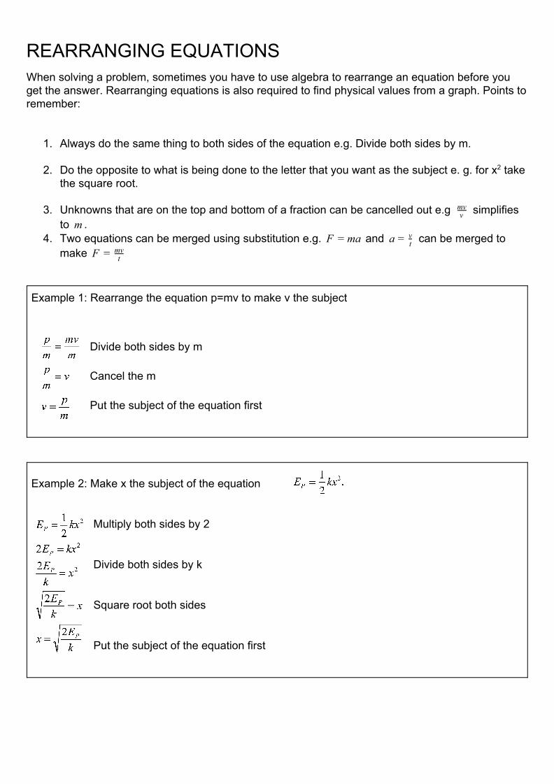
REARRANGING EQUATIONS When solving a problem, sometimes you have to use algebra to rearrange an equation before you get the answer. Rearranging equations is also required to find physical values from a graph. Points to remember:

1. Always do the same thing to both sides of the equation e.g. Divide both sides by m.

2. Do the opposite to what is being done to the letter that you want as the subject e. g. for x2 take the square root.

3. Unknowns that are on the top and bottom of a fraction can be cancelled out e.g simplifiesv

mv to .m

4. Two equations can be merged using substitution e.g. and can be merged toa F = m a = tv

make F = tmv

Example 1: Rearrange the equation p=mv to make v the subject

Divide both sides by m

Cancel the m

Put the subject of the equation first

Example 2: Make x the subject of the equation

Multiply both sides by 2

Divide both sides by k

Square root both sides

Put the subject of the equation first

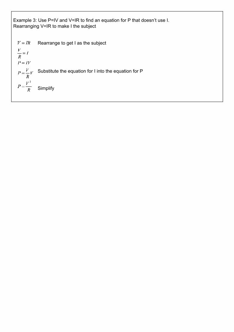
Example 3: Use P=IV and V=IR to find an equation for P that doesn’t use I. Rearranging V=IR to make I the subject

Rearrange to get I as the subject Substitute the equation for I into the equation for P

Simplify

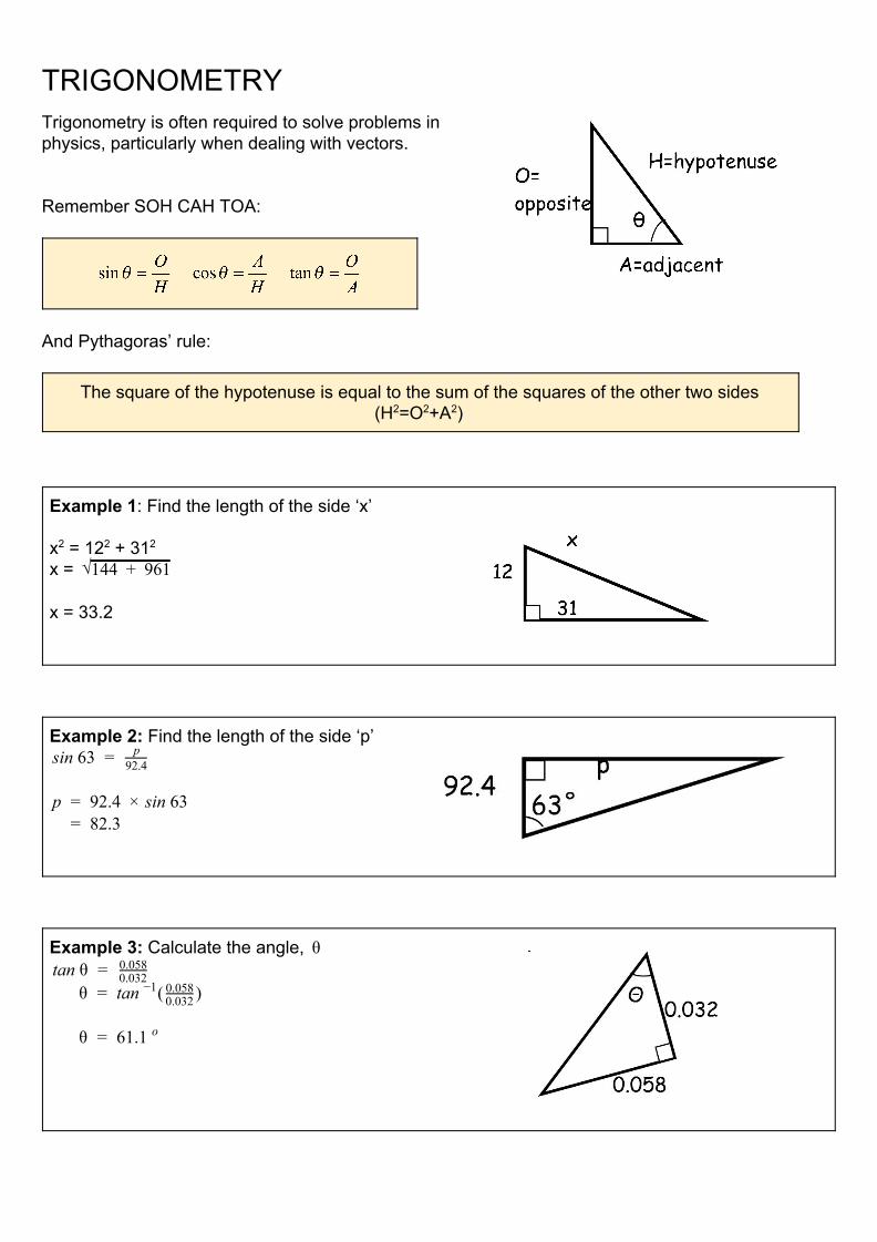
TRIGONOMETRY Trigonometry is often required to solve problems in physics, particularly when dealing with vectors. Remember SOH CAH TOA:

And Pythagoras’ rule:

The square of the hypotenuse is equal to the sum of the squares of the other two sides (H2=O2+A2)

Example 1: Find the length of the side ‘x’ x2 = 122 + 312

x = √144 961+ x = 33.2

Example 2: Find the length of the side ‘p’ in 63 s = p

92.4

92.4 p = × in 63 s 82.3 =

Example 3: Calculate the angle, θ an θ t = 0.032

0.058 θ tan ( ) = −1

0.0320.058

θ 61.1 = o

SCIENTIFIC NOTATION In science, one often has to deal with very large and very small numbers. Consider, for example, the mass of the Earth:

5 980 000 000 000 000 000 000 000 kg

This number is difficult to read, difficult to write, and difficult to say.

Scientific notation is an alternative way of expressing numbers. Here is the mass of the Earth written in scientific notation:

5.98 × 1024 kg

Clearly this is much easier to read and write. It is also easier to say:

“five point nine eight times ten to the power of 24 kilograms.”

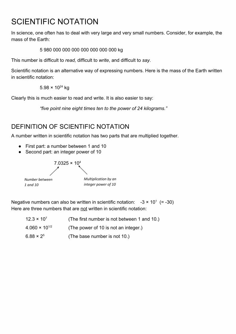
DEFINITION OF SCIENTIFIC NOTATION A number written in scientific notation has two parts that are multiplied together.

First part: a number between 1 and 10 Second part: an integer power of 10

7.0325 × 104

Negative numbers can also be written in scientific notation: -3 × 101 (= -30) Here are three numbers that are not written in scientific notation:

12.3 × 107 (The first number is not between 1 and 10.)

4.060 × 101/2 (The power of 10 is not an integer.)

6.88 × 25 (The base number is not 10.)

POWERS OF 10 Our number system is a base 10 system. Multiplying by powers of 10 is especially easy in a base 10 system:

10 × 10 = 100 10 × 10 × 10 = 1000 10 × 10 × 10 × 10 = 10 000 etc.

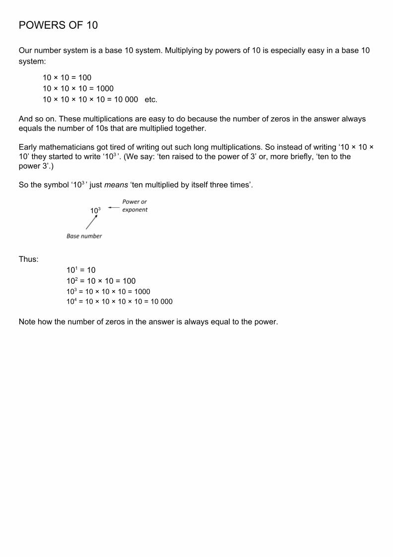
And so on. These multiplications are easy to do because the number of zeros in the answer always equals the number of 10s that are multiplied together. Early mathematicians got tired of writing out such long multiplications. So instead of writing ‘10 × 10 × 10’ they started to write ‘103 ’. (We say: ‘ten raised to the power of 3’ or, more briefly, ‘ten to the power 3’.) So the symbol ‘103 ’ just means ‘ten multiplied by itself three times’.

103

Thus: 101 = 10 102 = 10 × 10 = 100 103 = 10 × 10 × 10 = 1000 104 = 10 × 10 × 10 × 10 = 10 000

Note how the number of zeros in the answer is always equal to the power.

Multiplying by Powers of 10

Here is the rule for multiplying by ten:

To multiply a number by 10, move the decimal point one place to the right.

For example:

2.35 × 10 = 23.5

Whole numbers may without a decimal point. But it is easy to include one. For example:

674 × 10 = 674.0 × 10 = 6740 This rule is easily extended to multiplying by higher powers of ten:

To multiply a number by 102, move the decimal point two places to the right. To multiply a number by 103, move the decimal point three places to the right. To multiply a number by 104, move the decimal point four places to the right…

Some examples:

4.957 × 102 = 495.7

- 9 × 103 = - 9.000 × 103 = - 9 000

4.957 × 105 = 4.95700 × 105 = 495 700

CONVERTING TO AND FROM ORDINARY NUMBER NOTATION

Converting from Scientific Notation to Ordinary Number Notation

Look again at the last three examples. Notice how all the numbers on the left are in scientific notation, and all the numbers on the right are in ordinary number notation. This shows that we already know how to convert from scientific notation to ordinary number notation. Here is another example.

Example 1

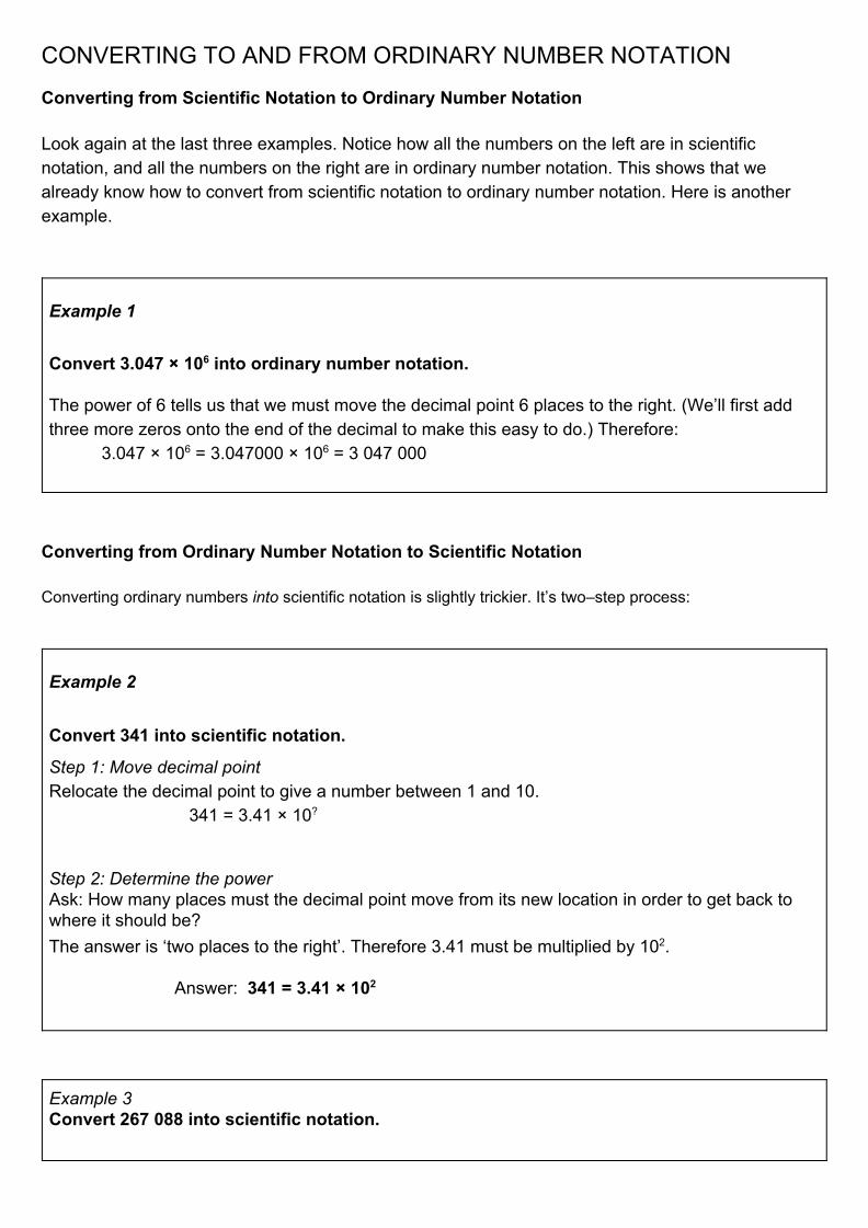
Convert 3.047 × 106 into ordinary number notation. The power of 6 tells us that we must move the decimal point 6 places to the right. (We’ll first add three more zeros onto the end of the decimal to make this easy to do.) Therefore:

3.047 × 106 = 3.047000 × 106 = 3 047 000

Converting from Ordinary Number Notation to Scientific Notation

Converting ordinary numbers into scientific notation is slightly trickier. It’s two–step process:

Example 2

Convert 341 into scientific notation.

Step 1: Move decimal point Relocate the decimal point to give a number between 1 and 10.

341 = 3.41 × 10?

Step 2: Determine the power Ask: How many places must the decimal point move from its new location in order to get back to where it should be?

The answer is ‘two places to the right’. Therefore 3.41 must be multiplied by 102.

Answer: 341 = 3.41 × 102

Example 3 Convert 267 088 into scientific notation.

Step 1: relocate the decimal point to give a number between 1 and 10:

267 088 = 2.67088 × 10?

Step 2: Ask: How many places must the decimal point move from its new location in order to get back to where it should be? Answer: five places to the right. Therefore: 267 088 = 2.67088 × 105

Numbers That Are Almost In Scientific Notation

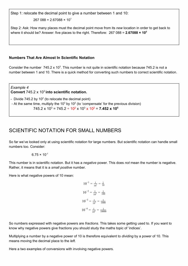
Consider the number 745.2 x 103. This number is not quite in scientific notation because 745.2 is not a number between 1 and 10. There is a quick method for converting such numbers to correct scientific notation.

Example 4 Convert 745.2 x 103 into scientific notation. - Divide 745.2 by 102 (to relocate the decimal point) - At the same time, multiply the 103 by 102 (to ‘compensate’ for the previous division)

745.2 x 103 = 745.2 ÷ 102 x 103 x 102 = 7.452 x 105

SCIENTIFIC NOTATION FOR SMALL NUMBERS

So far we’ve looked only at using scientific notation for large numbers. But scientific notation can handle small numbers too. Consider:

6.75 × 10-1

This number is in scientific notation. But it has a negative power. This does not mean the number is negative. Rather, it means that it is a small positive number.

Here is what negative powers of 10 mean:

10−1 = 1101 = 1

10

10−2 = 1102 = 1

100

10−3 = 1103 = 1

1000

10−4 = 1104 = 1

10000

So numbers expressed with negative powers are fractions. This takes some getting used to. If you want to know why negative powers give fractions you should study the maths topic of ‘indices’.

Multiplying a number by a negative power of 10 is therefore equivalent to dividing by a power of 10. This means moving the decimal place to the left.

Here a two examples of conversions with involving negative powers.

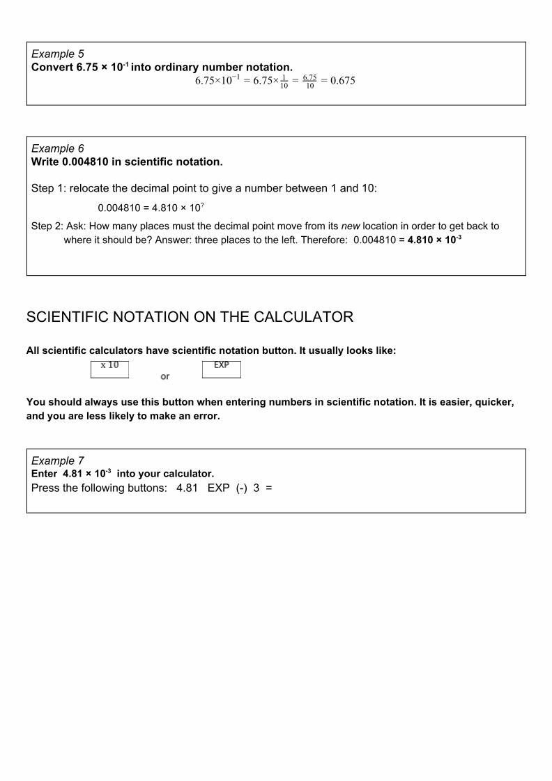
Example 5 Convert 6.75 × 10-1 into ordinary number notation.

.75×10 .75× .6756 −1 = 6 110 = 10

6.75 = 0

Example 6 Write 0.004810 in scientific notation. Step 1: relocate the decimal point to give a number between 1 and 10:

0.004810 = 4.810 × 10?

Step 2: Ask: How many places must the decimal point move from its new location in order to get back to where it should be? Answer: three places to the left. Therefore: 0.004810 = 4.810 × 10-3

SCIENTIFIC NOTATION ON THE CALCULATOR

All scientific calculators have scientific notation button. It usually looks like:

You should always use this button when entering numbers in scientific notation. It is easier, quicker, and you are less likely to make an error.

Example 7 Enter 4.81 × 10-3 into your calculator. Press the following buttons: 4.81 EXP (-) 3 =

SIGNIFICANT FIGURES

THE PURPOSE OF SIGNIFICANT FIGURES (SF)

No measurement is perfectly accurate. There are always limits to accuracy due to the limitations of measuring instruments. The purpose of SF is to indicate the level of accuracy of a measurement.

When reporting a measurement, the number of digits written indicates the level of accuracy. The relevant digits are referred to significant figures.

Example 1 (Reading a scale)

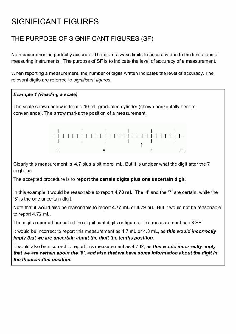
The scale shown below is from a 10 mL graduated cylinder (shown horizontally here for convenience). The arrow marks the position of a measurement.

Clearly this measurement is ‘4.7 plus a bit more’ mL. But it is unclear what the digit after the 7 might be.

The accepted procedure is to report the certain digits plus one uncertain digit. In this example it would be reasonable to report 4.78 mL. The ‘4’ and the ‘7’ are certain, while the ‘8’ is the one uncertain digit.

Note that it would also be reasonable to report 4.77 mL or 4.79 mL. But it would not be reasonable to report 4.72 mL.

The digits reported are called the significant digits or figures. This measurement has 3 SF.

It would be incorrect to report this measurement as 4.7 mL or 4.8 mL, as this would incorrectly imply that we are uncertain about the digit the tenths position.

It would also be incorrect to report this measurement as 4.782, as this would incorrectly imply that we are certain about the ’8’, and also that we have some information about the digit in the thousandths position.

RULES FOR DETERMINING SIGNIFICANT FIGURES

A Final Zero?

A measurement of 4.78 mL is not the same as a measurement of 4.780 mL. The extra zero on the end of the latter indicates that it was made to a higher degree of accuracy.

If your best estimate for the final digit is zero, you must write it down. The final zero at the end of a decimal number is always a significant digit.

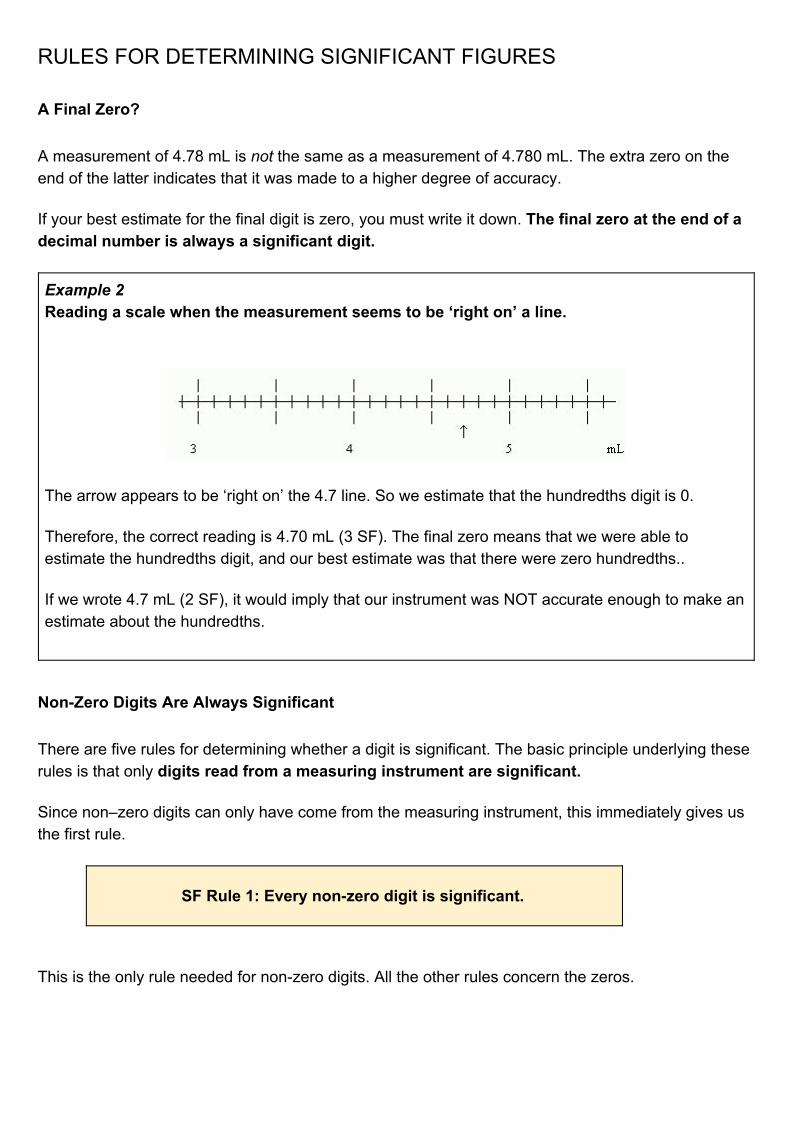
Example 2 Reading a scale when the measurement seems to be ‘right on’ a line.

The arrow appears to be ‘right on’ the 4.7 line. So we estimate that the hundredths digit is 0.

Therefore, the correct reading is 4.70 mL (3 SF). The final zero means that we were able to estimate the hundredths digit, and our best estimate was that there were zero hundredths..

If we wrote 4.7 mL (2 SF), it would imply that our instrument was NOT accurate enough to make an estimate about the hundredths.

Non-Zero Digits Are Always Significant

There are five rules for determining whether a digit is significant. The basic principle underlying these rules is that only digits read from a measuring instrument are significant.

Since non–zero digits can only have come from the measuring instrument, this immediately gives us the first rule.

SF Rule 1: Every non-zero digit is significant.

This is the only rule needed for non-zero digits. All the other rules concern the zeros.

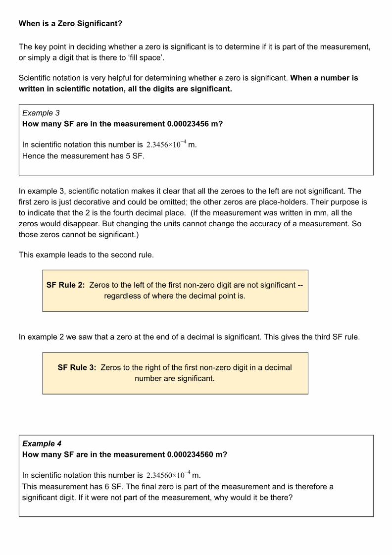
When is a Zero Significant?

The key point in deciding whether a zero is significant is to determine if it is part of the measurement, or simply a digit that is there to ‘fill space’.

Scientific notation is very helpful for determining whether a zero is significant. When a number is written in scientific notation, all the digits are significant.

Example 3 How many SF are in the measurement 0.00023456 m?

In scientific notation this number is m..3456×102 −4 Hence the measurement has 5 SF.

In example 3, scientific notation makes it clear that all the zeroes to the left are not significant. The first zero is just decorative and could be omitted; the other zeros are place-holders. Their purpose is to indicate that the 2 is the fourth decimal place. (If the measurement was written in mm, all the zeros would disappear. But changing the units cannot change the accuracy of a measurement. So those zeros cannot be significant.)

This example leads to the second rule.

SF Rule 2: Zeros to the left of the first non-zero digit are not significant -- regardless of where the decimal point is.

In example 2 we saw that a zero at the end of a decimal is significant. This gives the third SF rule.

SF Rule 3: Zeros to the right of the first non-zero digit in a decimal number are significant.

Example 4 How many SF are in the measurement 0.000234560 m?

In scientific notation this number is m..34560×102 −4 This measurement has 6 SF. The final zero is part of the measurement and is therefore a significant digit. If it were not part of the measurement, why would it be there?

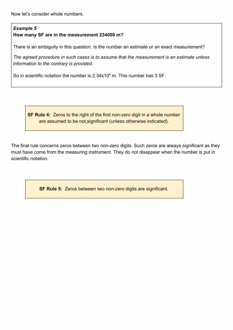
Now let’s consider whole numbers.

Example 5 How many SF are in the measurement 234000 m?

There is an ambiguity in this question. Is the number an estimate or an exact measurement?

The agreed procedure in such cases is to assume that the measurement is an estimate unless information to the contrary is provided.

So in scientific notation the number is 2.34x105 m. This number has 3 SF.

SF Rule 4: Zeros to the right of the first non-zero digit in a whole number are assumed to be not significant (unless otherwise indicated).

The final rule concerns zeros between two non-zero digits. Such zeros are always significant as they must have come from the measuring instrument. They do not disappear when the number is put in scientific notation.

SF Rule 5: Zeros between two non-zero digits are significant.

MEASUREMENT UNITS

Many scientific studies are based on experiments. Central to any experiment is the concept of measurement. When a scientist or engineer claims to have made a breakthrough, other researchers in the field want to know as many details as possible. Most importantly, they want quantitative or numerical information.

Numerical information allows researchers in other laboratories to make their own measurements which can then be compared with the original data. A starting point for such comparisons is a set of measurement units that everybody agrees upon.

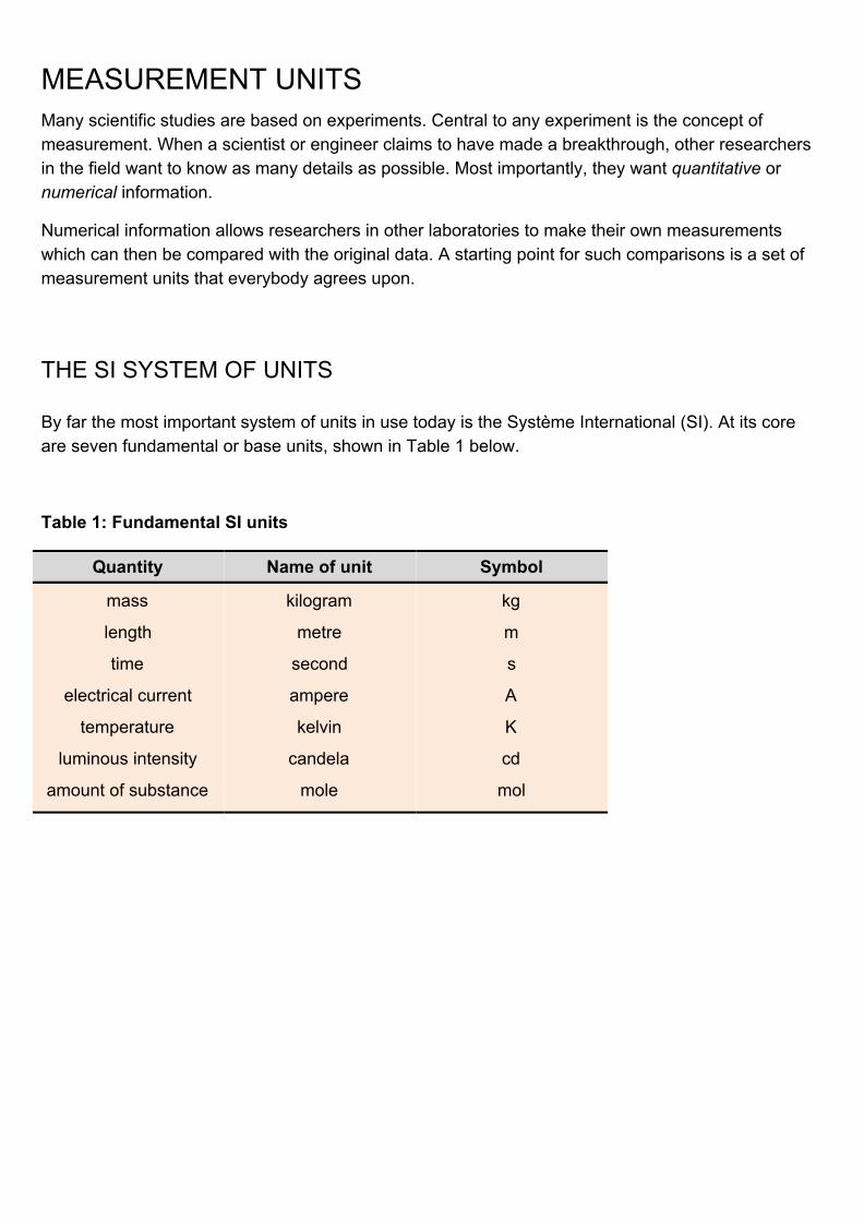
THE SI SYSTEM OF UNITS

By far the most important system of units in use today is the Système International (SI). At its core are seven fundamental or base units, shown in Table 1 below.

Table 1: Fundamental SI units

Quantity Name of unit Symbol

mass

length

time

electrical current

temperature

luminous intensity

amount of substance

kilogram

metre

second

ampere

kelvin

candela

mole

kg

m

s

A

K

cd

mol

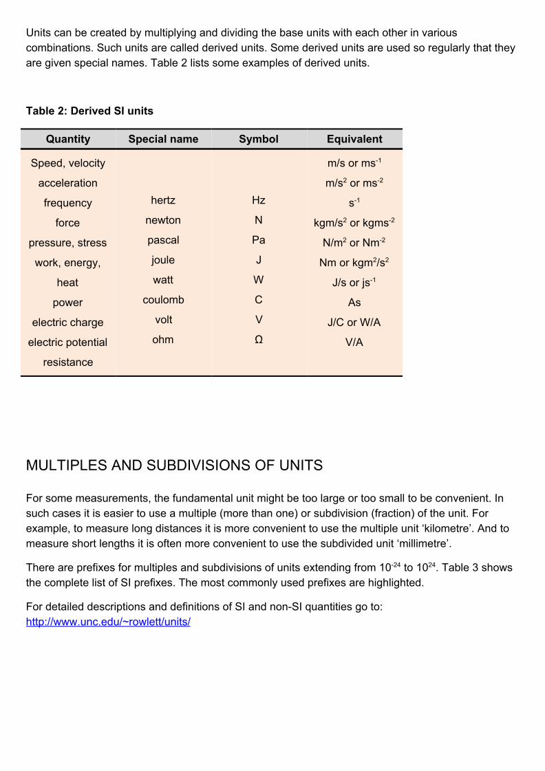
Units can be created by multiplying and dividing the base units with each other in various combinations. Such units are called derived units. Some derived units are used so regularly that they are given special names. Table 2 lists some examples of derived units.

Table 2: Derived SI units

Quantity Special name Symbol Equivalent

Speed, velocity

acceleration

frequency

force

pressure, stress

work, energy,

heat

power

electric charge

electric potential

resistance

hertz

newton

pascal

joule

watt

coulomb

volt

ohm

Hz

N

Pa

J

W

C

V

Ω

m/s or ms-1

m/s2 or ms-2

s-1

kgm/s2 or kgms-2

N/m2 or Nm-2

Nm or kgm2/s2

J/s or js-1

As

J/C or W/A

V/A

MULTIPLES AND SUBDIVISIONS OF UNITS

For some measurements, the fundamental unit might be too large or too small to be convenient. In such cases it is easier to use a multiple (more than one) or subdivision (fraction) of the unit. For example, to measure long distances it is more convenient to use the multiple unit ‘kilometre’. And to measure short lengths it is often more convenient to use the subdivided unit ‘millimetre’.

There are prefixes for multiples and subdivisions of units extending from 10-24 to 1024. Table 3 shows the complete list of SI prefixes. The most commonly used prefixes are highlighted.

For detailed descriptions and definitions of SI and non-SI quantities go to: http://www.unc.edu/~rowlett/units/

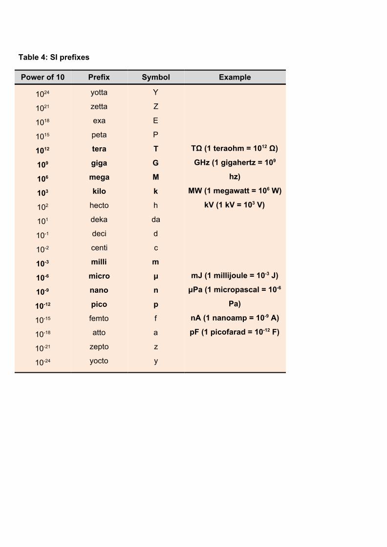
Table 4: SI prefixes

Power of 10 Prefix Symbol Example

1024

1021

1018

1015

1012

109

106

103

102

101

10-1

10-2

10-3

10-6

10-9

10-12

10-15

10-18

10-21

10-24

yotta

zetta

exa

peta

tera

giga

mega

kilo

hecto

deka

deci

centi

milli

micro

nano

pico

femto

atto

zepto

yocto

Y

Z

E

P

T

G

M

k

h

da

d

c

m

μ

n

p

f

a

z

y

TΩ (1 teraohm = 1012 Ω)

GHz (1 gigahertz = 109

hz)

MW (1 megawatt = 106 W)

kV (1 kV = 103 V)

mJ (1 millijoule = 10-3 J)

μPa (1 micropascal = 10-6

Pa)

nA (1 nanoamp = 10-9 A)

pF (1 picofarad = 10-12 F)

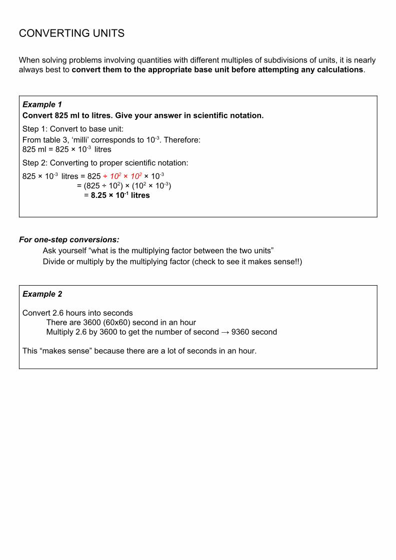
CONVERTING UNITS

When solving problems involving quantities with different multiples of subdivisions of units, it is nearly always best to convert them to the appropriate base unit before attempting any calculations.

Example 1 Convert 825 ml to litres. Give your answer in scientific notation. Step 1: Convert to base unit: From table 3, ‘milli’ corresponds to 10-3. Therefore: 825 ml = 825 × 10-3 litres Step 2: Converting to proper scientific notation: 825 × 10-3 litres = 825 ÷ 102 × 102 × 10-3

= (825 ÷ 102) × (102 × 10-3) = 8.25 × 10-1 litres

For one-step conversions: Ask yourself “what is the multiplying factor between the two units” Divide or multiply by the multiplying factor (check to see it makes sense!!)

Example 2 Convert 2.6 hours into seconds

There are 3600 (60x60) second in an hour Multiply 2.6 by 3600 to get the number of second → 9360 second

This “makes sense” because there are a lot of seconds in an hour.

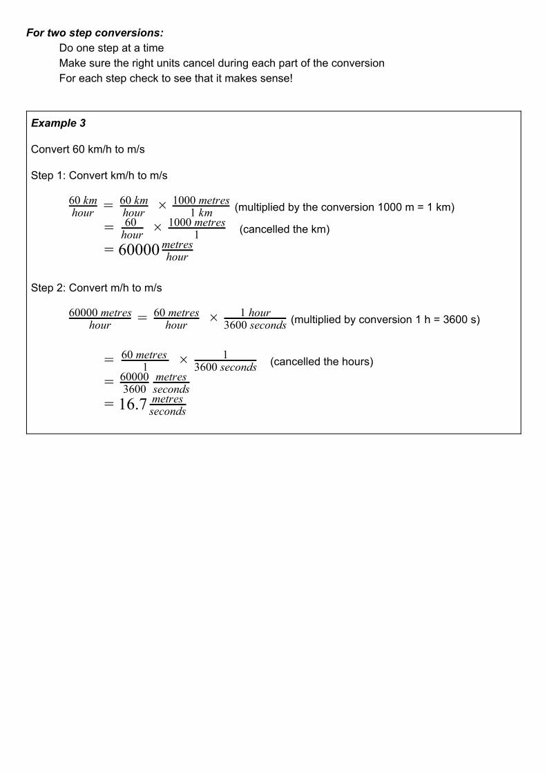
For two step conversions: Do one step at a time Make sure the right units cancel during each part of the conversion For each step check to see that it makes sense!

Example 3 Convert 60 km/h to m/s Step 1: Convert km/h to m/s

(multiplied by the conversion 1000 m = 1 km) hour60 km = hour

60 km × 1 km1000 metres

(cancelled the km) = 60 hour × 1

1000 metres

0000 = 6 hourmetres

Step 2: Convert m/h to m/s

(multiplied by conversion 1 h = 3600 s) hour60000 metres = hour

60 metres × 1 hour3600 seconds

(cancelled the hours) = 1

60 metres × 13600 seconds

= 360060000 metres

seconds 6.7 = 1 metres

seconds

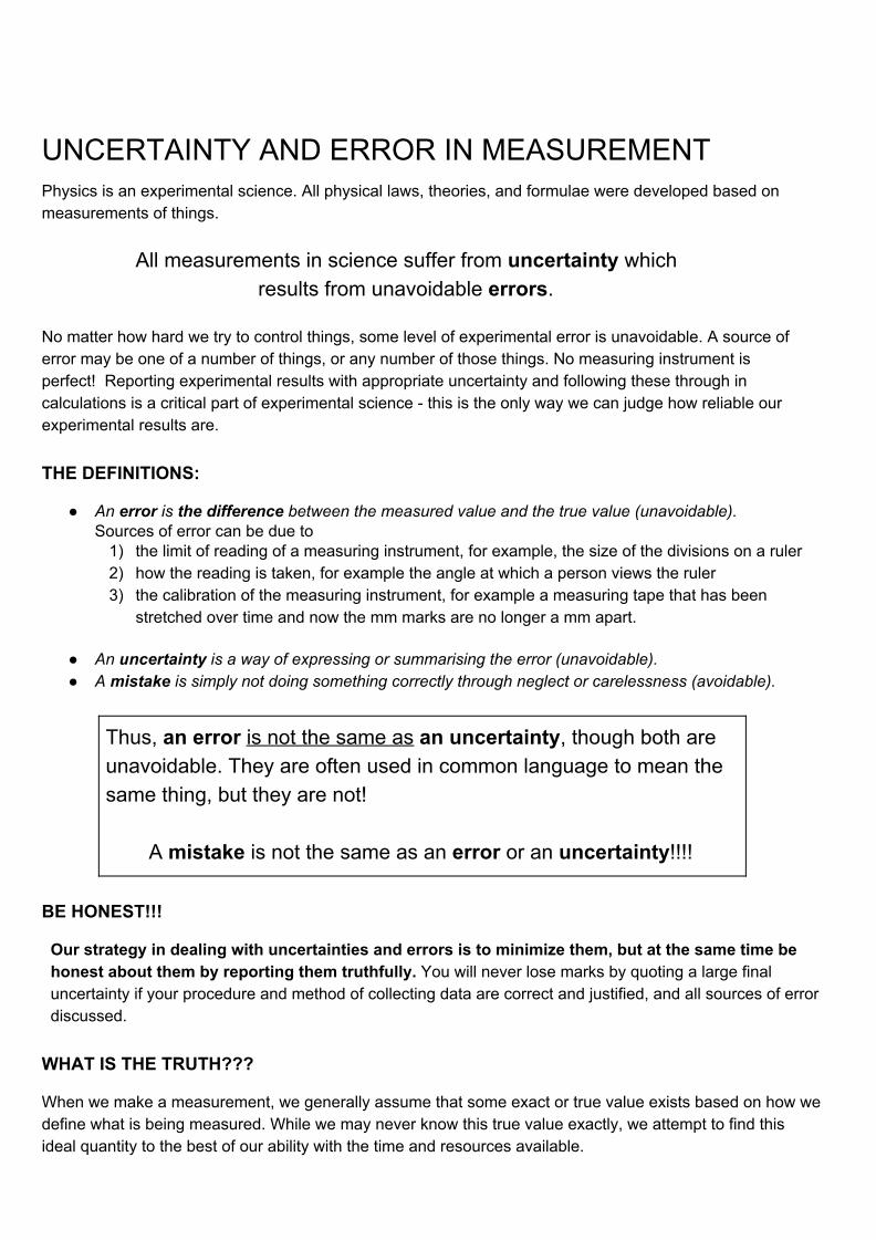
UNCERTAINTY AND ERROR IN MEASUREMENT Physics is an experimental science. All physical laws, theories, and formulae were developed based on measurements of things.

All measurements in science suffer from uncertainty which results from unavoidable errors.

No matter how hard we try to control things, some level of experimental error is unavoidable. A source of error may be one of a number of things, or any number of those things. No measuring instrument is perfect! Reporting experimental results with appropriate uncertainty and following these through in calculations is a critical part of experimental science - this is the only way we can judge how reliable our experimental results are. THE DEFINITIONS:

An error is the difference between the measured value and the true value (unavoidable). Sources of error can be due to

1) the limit of reading of a measuring instrument, for example, the size of the divisions on a ruler 2) how the reading is taken, for example the angle at which a person views the ruler 3) the calibration of the measuring instrument, for example a measuring tape that has been

stretched over time and now the mm marks are no longer a mm apart.

An uncertainty is a way of expressing or summarising the error (unavoidable). A mistake is simply not doing something correctly through neglect or carelessness (avoidable).

Thus, an error is not the same as an uncertainty, though both are unavoidable. They are often used in common language to mean the same thing, but they are not!

A mistake is not the same as an error or an uncertainty!!!! BE HONEST!!!

Our strategy in dealing with uncertainties and errors is to minimize them, but at the same time be honest about them by reporting them truthfully. You will never lose marks by quoting a large final uncertainty if your procedure and method of collecting data are correct and justified, and all sources of error discussed.

WHAT IS THE TRUTH???

When we make a measurement, we generally assume that some exact or true value exists based on how we define what is being measured. While we may never know this true value exactly, we attempt to find this ideal quantity to the best of our ability with the time and resources available.

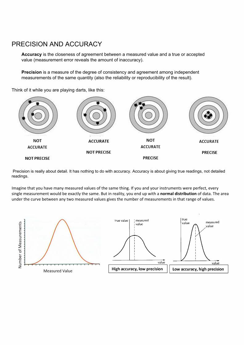
PRECISION AND ACCURACY Accuracy is the closeness of agreement between a measured value and a true or accepted value (measurement error reveals the amount of inaccuracy).

Precision is a measure of the degree of consistency and agreement among independent measurements of the same quantity (also the reliability or reproducibility of the result).

Think of it while you are playing darts, like this:

Precision is really about detail. It has nothing to do with accuracy. Accuracy is about giving true readings, not detailed readings. Imagine that you have many measured values of the same thing. If you and your instruments were perfect, every single measurement would be exactly the same. But in reality, you end up with a normal distribution of data. The area under the curve between any two measured values gives the number of measurements in that range of values.

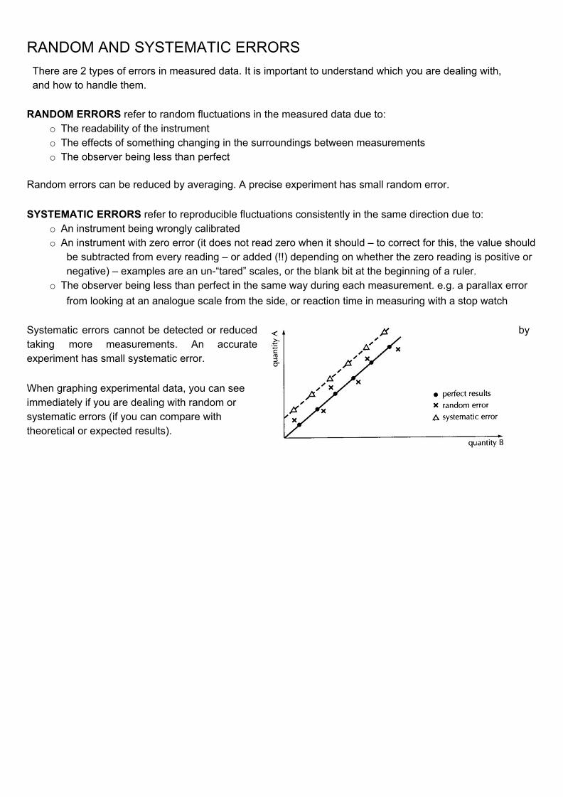
RANDOM AND SYSTEMATIC ERRORS There are 2 types of errors in measured data. It is important to understand which you are dealing with, and how to handle them.

RANDOM ERRORS refer to random fluctuations in the measured data due to:

o The readability of the instrument o The effects of something changing in the surroundings between measurements o The observer being less than perfect

Random errors can be reduced by averaging. A precise experiment has small random error. SYSTEMATIC ERRORS refer to reproducible fluctuations consistently in the same direction due to:

o An instrument being wrongly calibrated o An instrument with zero error (it does not read zero when it should – to correct for this, the value should

be subtracted from every reading – or added (!!) depending on whether the zero reading is positive or negative) – examples are an un-“tared” scales, or the blank bit at the beginning of a ruler.

o The observer being less than perfect in the same way during each measurement. e.g. a parallax error from looking at an analogue scale from the side, or reaction time in measuring with a stop watch

Systematic errors cannot be detected or reduced by taking more measurements. An accurate experiment has small systematic error. When graphing experimental data, you can see immediately if you are dealing with random or systematic errors (if you can compare with theoretical or expected results).

EXPERIMENTAL TECHNIQUES TO MAXIMISE ACCURACY AND PRECISION There are lots of different techniques that can be used in different experiments that will help improve the precision and accuracy of your measurements. These include, but are not limited to:

- Taking readings straight on to minimise parallax - Taking repeated readings - Taking zero readings - Taking multiple readings - Choosing the appropriate scale for the size of the variable that you are measuring.

When planning experiments, you will need to be aware of the techniques you use and why you use them. Below are some examples for different measurement types, but your individual experiments may require these and other techniques to get the best data.

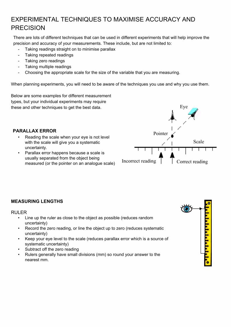
PARALLAX ERROR • Reading the scale when your eye is not level

with the scale will give you a systematic uncertainty.

• Parallax error happens because a scale is usually separated from the object being measured (or the pointer on an analogue scale)

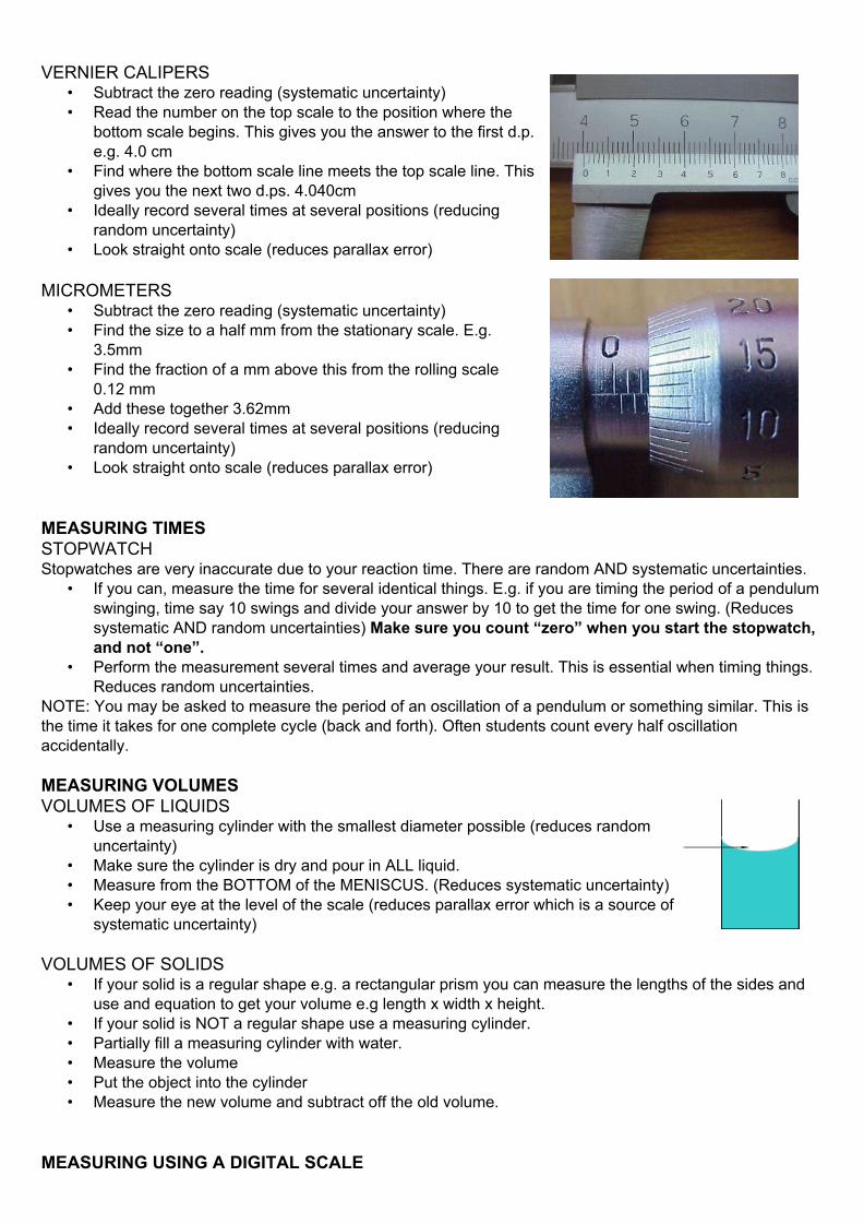
MEASURING LENGTHS RULER

• Line up the ruler as close to the object as possible (reduces random uncertainty)

• Record the zero reading, or line the object up to zero (reduces systematic uncertainty)

• Keep your eye level to the scale (reduces parallax error which is a source of systematic uncertainty)

• Subtract off the zero reading • Rulers generally have small divisions (mm) so round your answer to the

nearest mm.

VERNIER CALIPERS

• Subtract the zero reading (systematic uncertainty) • Read the number on the top scale to the position where the

bottom scale begins. This gives you the answer to the first d.p. e.g. 4.0 cm

• Find where the bottom scale line meets the top scale line. This gives you the next two d.ps. 4.040cm

• Ideally record several times at several positions (reducing random uncertainty)

• Look straight onto scale (reduces parallax error) MICROMETERS

• Subtract the zero reading (systematic uncertainty) • Find the size to a half mm from the stationary scale. E.g.

3.5mm • Find the fraction of a mm above this from the rolling scale

0.12 mm • Add these together 3.62mm • Ideally record several times at several positions (reducing

random uncertainty) • Look straight onto scale (reduces parallax error)

MEASURING TIMES STOPWATCH Stopwatches are very inaccurate due to your reaction time. There are random AND systematic uncertainties.

• If you can, measure the time for several identical things. E.g. if you are timing the period of a pendulum swinging, time say 10 swings and divide your answer by 10 to get the time for one swing. (Reduces systematic AND random uncertainties) Make sure you count “zero” when you start the stopwatch, and not “one”.

• Perform the measurement several times and average your result. This is essential when timing things. Reduces random uncertainties.

NOTE: You may be asked to measure the period of an oscillation of a pendulum or something similar. This is the time it takes for one complete cycle (back and forth). Often students count every half oscillation accidentally. MEASURING VOLUMES VOLUMES OF LIQUIDS

• Use a measuring cylinder with the smallest diameter possible (reduces random uncertainty)

• Make sure the cylinder is dry and pour in ALL liquid. • Measure from the BOTTOM of the MENISCUS. (Reduces systematic uncertainty) • Keep your eye at the level of the scale (reduces parallax error which is a source of

systematic uncertainty) VOLUMES OF SOLIDS

• If your solid is a regular shape e.g. a rectangular prism you can measure the lengths of the sides and use and equation to get your volume e.g length x width x height.

• If your solid is NOT a regular shape use a measuring cylinder. • Partially fill a measuring cylinder with water. • Measure the volume • Put the object into the cylinder • Measure the new volume and subtract off the old volume.

MEASURING USING A DIGITAL SCALE

• E.g. mass balance or multimeter. If possible switch to the range that gives you the most accurate measurement. (Reduces random uncertainty)

• Zero the scale before taking a reading OR record the zero reading (reduces systematic uncertainty) • If possible measure several items and then divide. E.g. to measure the mass of a paper clip measure

the mass of 50 paper clips then divide by 50. (Reduces random uncertainty) MEASURING USING AN ANALOGUE SCALE

• E.g. bathroom scales, ammeter or voltmeter. • Zero the scale before taking a reading OR record the zero reading (reduces systematic uncertainty) • Read the scale from straight on (reduces parallax error) • Estimate IN BETWEEN the divisions in the scale as most analogue scales have big divisions. • If possible measure several items and then divide. E.g. to measure the mass of a paper clip measure

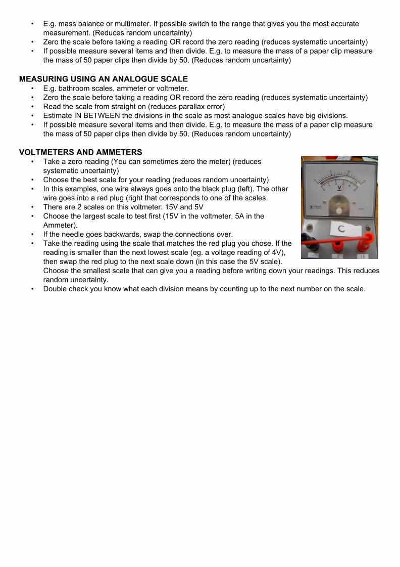
the mass of 50 paper clips then divide by 50. (Reduces random uncertainty) VOLTMETERS AND AMMETERS

• Take a zero reading (You can sometimes zero the meter) (reduces systematic uncertainty)

• Choose the best scale for your reading (reduces random uncertainty) • In this examples, one wire always goes onto the black plug (left). The other

wire goes into a red plug (right that corresponds to one of the scales. • There are 2 scales on this voltmeter: 15V and 5V • Choose the largest scale to test first (15V in the voltmeter, 5A in the

Ammeter). • If the needle goes backwards, swap the connections over. • Take the reading using the scale that matches the red plug you chose. If the

reading is smaller than the next lowest scale (eg. a voltage reading of 4V), then swap the red plug to the next scale down (in this case the 5V scale). Choose the smallest scale that can give you a reading before writing down your readings. This reduces random uncertainty.

• Double check you know what each division means by counting up to the next number on the scale.

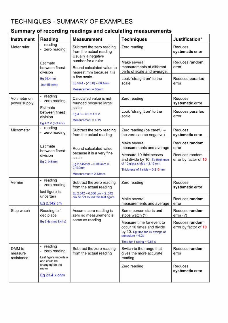
TECHNIQUES - SUMMARY OF EXAMPLES Summary of recording readings and calculating measurements Instrument Reading Measurement Techniques Justification* Meter ruler - reading

- zero reading.

Estimate between finest division Eg 56.4mm

(not 56 mm)

Subtract the zero reading from the actual reading Usually a negative number for a ruler

Round calculated value to nearest mm because it is a fine scale. Eg 56.4 - (-10.0) = 66.4mm

Measurement = 66mm

Zero reading

Reduces systematic error

Make several measurements at different parts of scale and average.

Reduces random error.

Look “straight on” to the scale

Reduces parallax error

Voltmeter on power supply

- reading - zero reading.

Estimate between finest division Eg 4.3 V (not 4 V)

Calculated value is not rounded because large scale. Eg 4.3 – 0.2 = 4.1 V

Measurement = 4.1V

Zero reading Reduces systematic error

Look “straight on” to the scale

Reduces parallax error

Micrometer - reading - zero reading.

Estimate between finest division Eg 2.145mm

Subtract the zero reading from the actual reading

Round calculated value because it is a very fine scale. Eg 2.145mm – 0.015mm = 2.130mm

Measurement= 2.13mm

Zero reading (be careful – the zero can be negative)

Reduces systematic error

Make several measurements and average

Reduces random error

Measure 10 thicknesses and divide by 10. Eg thickness of 10 glass slides = 2.13 mm

Thickness of 1 slide = 0.213mm

Reduces random error by factor of 10

Vernier - reading - zero reading.

last figure is uncertain

Eg 2.342 cm

Subtract the zero reading from the actual reading Eg 2.342 – 0.000 cm = 2..342 cm do not round this last figure

Zero reading

Reduces systematic error

Make several measurements and average

Reduces random error

Stop watch Reading to 1 dec place Eg 3.4s (not 3.41s)

Assume zero reading is zero so measurement is same as reading

Same person starts and stops watch (?)

Reduces random error (?)

Measure time for event to occur 10 times and divide by 10. Eg time for 10 swings of pendulum = 6.3s

Time for 1 swing = 0.63 s

Reduces random error by factor of 10

DMM to measure resistance

- reading - zero reading. Last figure uncertain and could be changing on the meter

Eg 23.4 k ohm

Subtract the zero reading from the actual reading

Switch to the range that gives the more accurate reading.

Reduces random error

Zero reading

Reduces systematic error

TECHNIQUES - SAMPLE EXPLANATIONS You need the units correct and an accurate measurement for 3/5 tasks to get A. You also need to state your measured value to an appropriate number of significant figures. 1. Measure the period of a mass oscillating on a spring. Period is given in seconds.

• Write final measurement with reasonable significant figures. • E.g. if the first time you got a period of 0.567s and the second time you got a period of 0.558 then write

your answer as 0.56 rather than 0.5625. Techniques: I measured the time for 10 oscillations (or some other number) and divided by 10 to get period

why? – hard to time accurately one oscillation as it is too quick. Will reduce systematic and random uncertainties associated with my reaction time. The measurement can therefore be quoted to a larger number of significant figures.

I made the measurement several times and average the results why? this will reduce the random uncertainty associated with reaction time. Averaging several measurements will reduce this uncertainty.

I knelt down so my eye was level with the mass at the bottom of its oscillation why? this reduces parallax error by ensuring I started and stopped the stopwatch accurately at the same point of the oscillation.

2. Thickness of a slide/book using micrometer/vernier caliper. Thickness is given in mm (micrometer) or cm (veriner calliper).

• Write readings with correct significant figures • For micrometer readings, estimate between divisions then round after zero reading subtracted.

Techniques: I made the a thickness reading at several places and averaged the results

why? this will reduce the random uncertainty associated with variations in the thickness of the object. Averaging several measurements will reduce this uncertainty.

I took a zero reading and subtracted this from the actual reading why? – to reduce the systematic uncertainty associated with the vernier calliper / micrometer not reading zero when it is closed.

I looked directly onto the scale why? this reduces parallax error in reading the scale

3. Measure the rebound height of a ball when it is dropped a distance of 1m. Height in metres, centimetres or millimetres. Write the answer to appropriate significant figures. Techniques I took several readings and averaged the results

why? it is hard to measure the height of the ball’s bounce as it is only at the top point of it’s path for a short time. Averaging reduces the random uncertainty involved in taking this quick reading.

I put my eye level with the ball’s bounce why? To reduce parallax error (a systematic uncertainty) caused by separation between the ball at the scale. I could then measure more accurately where on the ruler the ball reached.

I measured from the bottom of the ball why? so I was measuring the total change in distance of the ball, not the bounce+ the height of the ball, thus reducing this systematic uncertainty

I made sure the ruler was vertical by lining it up with the bench why? this reduces systematic uncertainty. If the ruler was not vertical I would always measure a slightly bigger result than the real result.

I subtracted the zero reading when raising the ball to 100cm. When dropping the ball I placed the bottom of the ball at 99.5cm level

why? The ruler has 5mm at the end (note: each ruler is different). This reduces systematic uncertainty. If I didn’t do this I would always be dropping it 5mm too high.

I added 0.5cm to all results. why? The ruler has 5mm zero reading at the end. This reduces systematic uncertainty as if I didn’t I would be measuring the bounce to be 5mm too small.

4. Measure the mass of a drawing pin Mass in grams Round to an appropriate number of significant figures Techniques I measured the mass of 50 drawing pins and divided the result by 50.

why? the scale isn’t accurate enough to measure 1 drawing pin accurately. Measuring several reduces the random uncertainty and you get more significant figures (better precision) in the answer.

I zeroed the electronic scale why? to remove the systematic uncertainty of a non-zero reading before the mass was added.

I counted the 50 drawing pins again and repeated my measurement the mass. why? Check that I had the correct number of pins and checked my measurement of the balance was not variable.

5. Measure the volume of a whiteboard marker Volume in mls. Round to an appropriate number of significant figures Techniques I took the reading of water before the pen went into it

why? this is the zero reading. If I didn’t do this my value would be the combined volume of water and pen.

I always kept my eye level to the scale and read from the bottom of the meniscus. why? reduces parallax error and the systematic uncertainty that would have arisen if I measured from the top of the meniscus.

I dried the pen and repeated the reading with a new set up why? checks that the first result is correct (if variable – repeat again and average then describe in your

write-up) 6. Measure the voltage across a battery Voltage in Volts Round to an appropriate number of significant figures. Techniques I chose the 0-5V scale rather than the 0-15V scale

why? more precise scale as divisions are smaller. Ensured that when the wires were apart the voltage read zero/subtracted off the zero reading

why? Reduced systematic uncertainty due to zero error. Kept wires firmly onto the battery and waited until the needle was stationary

why? the voltage would not be correct if the wires were not on firmly. I repeated the measurement twice

why? To check whether the voltage reading changed (if it does change then you would do more repeat measurements and average…) 7. Measure the resistance of a wire with a multimeter. Resistance in Ohms Ω Round to an appropriate number of significant figures. I put the multimeter to the most appropriate scale (on the resistance setting (Ω or kΩ)) by starting at the largest scale then moving down.

why? so it gave the most precise reading for the given resistor. I checked the zero reading by touching the crocodile clips together.

why? reduces systematic uncertainty due to zero error produced by internal resistance of the circuit. I measured the resistance 3 times each time replacing the crocodile clips.

why? To reduce systematic uncertainties from the clips not being firmly on the resistor.

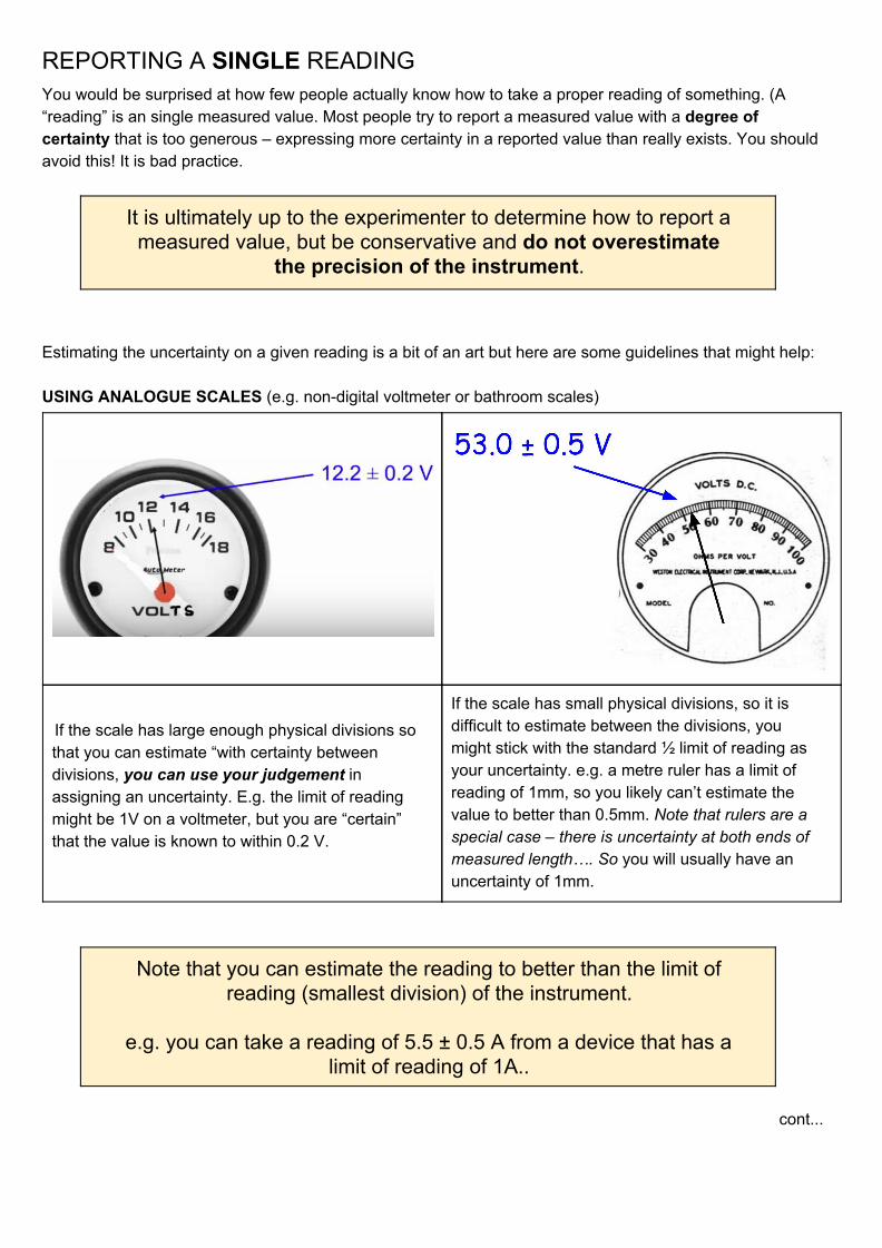
REPORTING A SINGLE READING You would be surprised at how few people actually know how to take a proper reading of something. (A “reading” is an single measured value. Most people try to report a measured value with a degree of certainty that is too generous – expressing more certainty in a reported value than really exists. You should avoid this! It is bad practice.

It is ultimately up to the experimenter to determine how to report a measured value, but be conservative and do not overestimate

the precision of the instrument.

Estimating the uncertainty on a given reading is a bit of an art but here are some guidelines that might help: USING ANALOGUE SCALES (e.g. non-digital voltmeter or bathroom scales)

If the scale has large enough physical divisions so that you can estimate “with certainty between divisions, you can use your judgement in assigning an uncertainty. E.g. the limit of reading might be 1V on a voltmeter, but you are “certain” that the value is known to within 0.2 V.

If the scale has small physical divisions, so it is difficult to estimate between the divisions, you might stick with the standard ½ limit of reading as your uncertainty. e.g. a metre ruler has a limit of reading of 1mm, so you likely can’t estimate the value to better than 0.5mm. Note that rulers are a special case – there is uncertainty at both ends of measured length…. So you will usually have an uncertainty of 1mm.

Note that you can estimate the reading to better than the limit of reading (smallest division) of the instrument.

e.g. you can take a reading of 5.5 ± 0.5 A from a device that has a

limit of reading of 1A..

cont...

USING DIGITAL SCALES (e.g. digital scales) In general the uncertainty for a reading made on digital scales is equal to the smallest division of the scale. (It is meaningless to quote the uncertainty to more decimal places than you can quote the reading itself). e.g. if the scales give a reading of 1.083g, the uncertainty would be 0.001g, so 1.083 ± 0.001 g USING STANDARD MASSES (mass) So-called ‘standard masses’ are less accurate than you would think, and vary considerably. Generally consider the uncertainty to be 1%. So, 100 g = 100 ± 1 g, 1.0 kg = 1000 ± 10 g, etc. USING STOPWATCHES (time) Most (but not all) stopwatches report to the 0.01 s. Since this is a digital scale, the instrumental uncertainty would be equal to the smallest division - in this case 0.01s. However, taking this least count as the uncertainty is ridiculous since you could never, ever move your thumb that fast! You can get a better estimate of the uncertainty on your timing measurements by taking repeated readings and looking at the spread of the data.

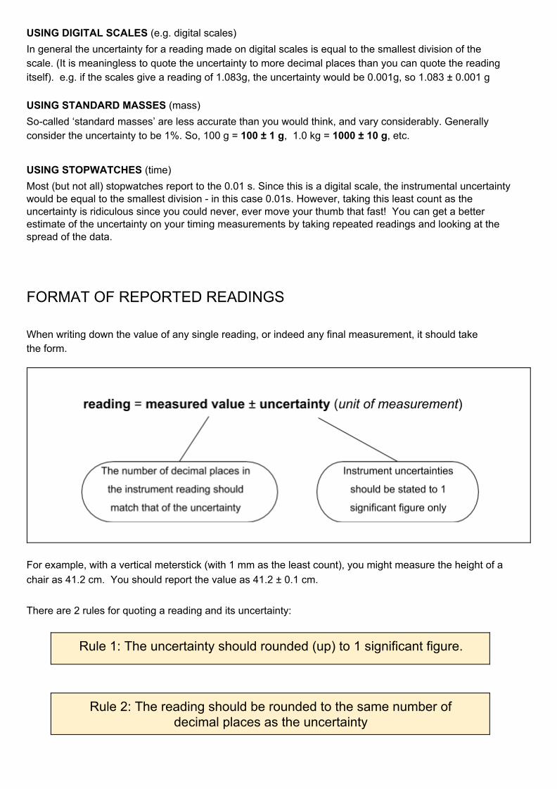
FORMAT OF REPORTED READINGS When writing down the value of any single reading, or indeed any final measurement, it should take the form.

For example, with a vertical meterstick (with 1 mm as the least count), you might measure the height of a chair as 41.2 cm. You should report the value as 41.2 ± 0.1 cm. There are 2 rules for quoting a reading and its uncertainty:

Rule 1: The uncertainty should rounded (up) to 1 significant figure.

Rule 2: The reading should be rounded to the same number of decimal places as the uncertainty

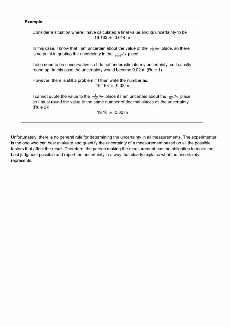
Example: Consider a situation where I have calculated a final value and its uncertainty to be

19.163 0.014 m± In this case, I know that I am uncertain about the value of the place, so thereths1

100 is no point in quoting the uncertainty in the placeths1

1000 I also need to be conservative so I do not underestimate my uncertainty, so I usually round up. In this case the uncertainty would become 0.02 m (Rule 1). However, there is still a problem if I then write the number as:

19.163 0.02 m±

I cannot quote the value to the place if I am uncertain about the place,ths11000 ths1

100 so I must round the value to the same number of decimal places as the uncertainty (Rule 2):

19.16 0.02 m±

Unfortunately, there is no general rule for determining the uncertainty in all measurements. The experimenter is the one who can best evaluate and quantify the uncertainty of a measurement based on all the possible factors that affect the result. Therefore, the person making the measurement has the obligation to make the best judgment possible and report the uncertainty in a way that clearly explains what the uncertainty represents.

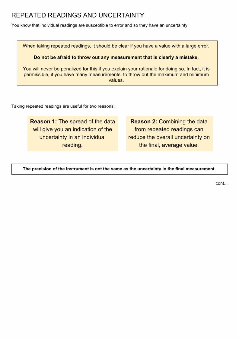
REPEATED READINGS AND UNCERTAINTY You know that individual readings are susceptible to error and so they have an uncertainty.

When taking repeated readings, it should be clear if you have a value with a large error.

Do not be afraid to throw out any measurement that is clearly a mistake.

You will never be penalized for this if you explain your rationale for doing so. In fact, it is permissible, if you have many measurements, to throw out the maximum and minimum

values. Taking repeated readings are useful for two reasons:

Reason 1: The spread of the data will give you an indication of the

uncertainty in an individual reading.

Reason 2: Combining the data from repeated readings can

reduce the overall uncertainty on the final, average value.

The precision of the instrument is not the same as the uncertainty in the final measurement.

cont...

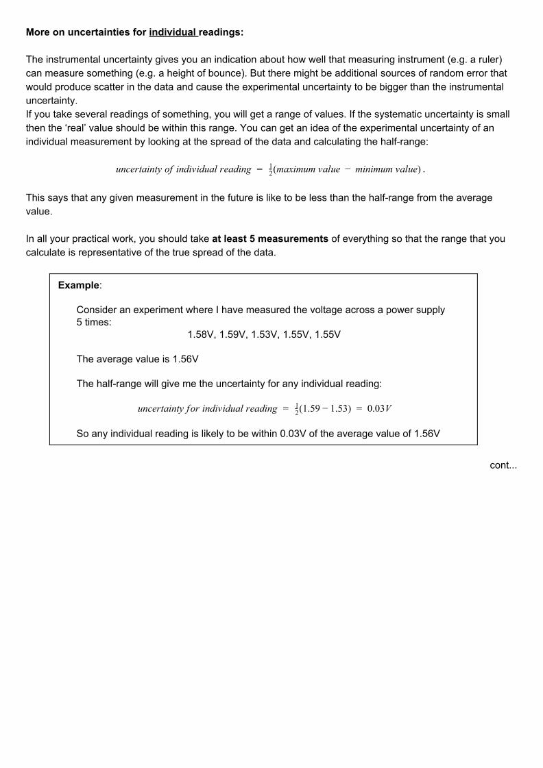
More on uncertainties for individual readings: The instrumental uncertainty gives you an indication about how well that measuring instrument (e.g. a ruler) can measure something (e.g. a height of bounce). But there might be additional sources of random error that would produce scatter in the data and cause the experimental uncertainty to be bigger than the instrumental uncertainty. If you take several readings of something, you will get a range of values. If the systematic uncertainty is small then the ‘real’ value should be within this range. You can get an idea of the experimental uncertainty of an individual measurement by looking at the spread of the data and calculating the half-range:

.ncertainty of individual reading (maximum value minimum value)u = 21 −

This says that any given measurement in the future is like to be less than the half-range from the average value. In all your practical work, you should take at least 5 measurements of everything so that the range that you calculate is representative of the true spread of the data.

Example: Consider an experiment where I have measured the voltage across a power supply 5 times:

1.58V, 1.59V, 1.53V, 1.55V, 1.55V The average value is 1.56V The half-range will give me the uncertainty for any individual reading:

ncertainty for individual reading (1.59 .53) 0.03Vu = 21 − 1 =

So any individual reading is likely to be within 0.03V of the average value of 1.56V

cont...

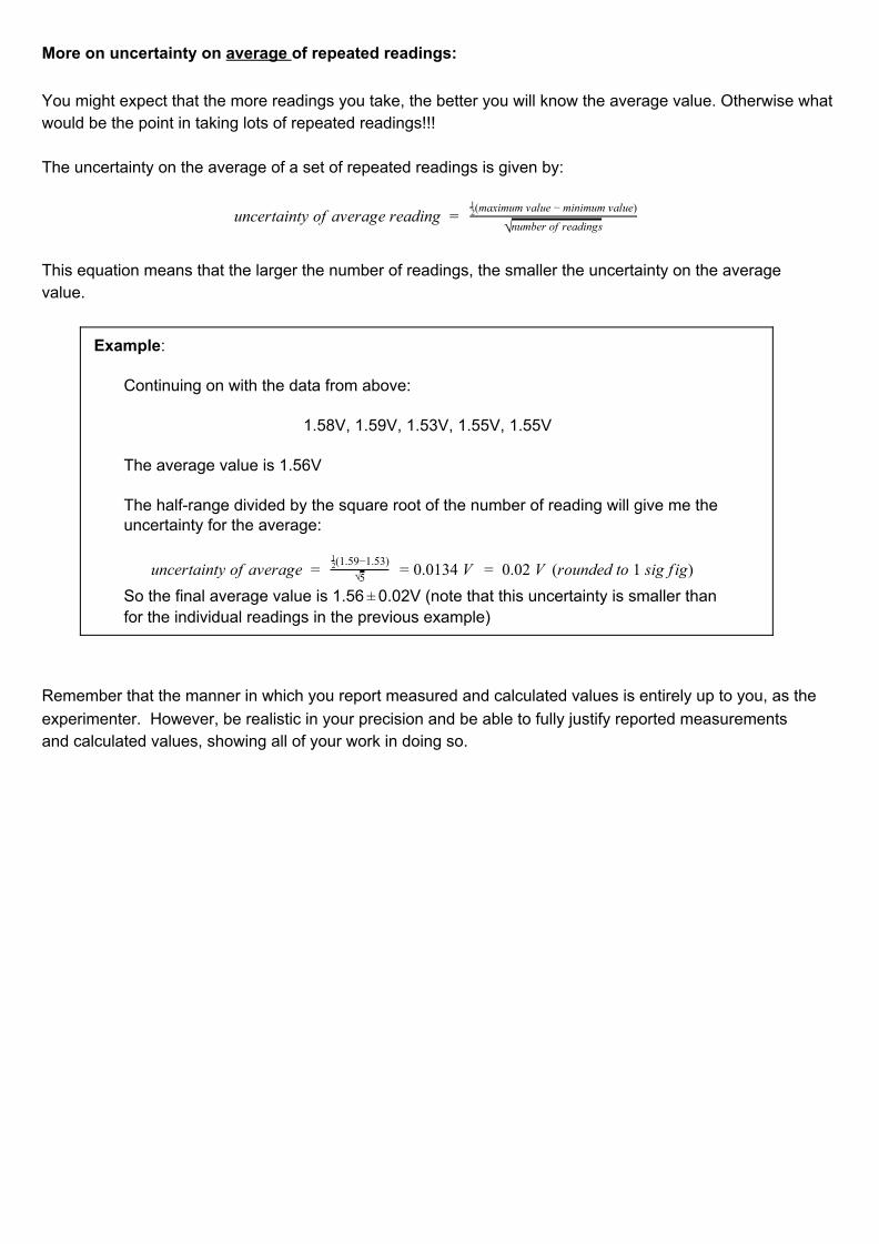
More on uncertainty on average of repeated readings: You might expect that the more readings you take, the better you will know the average value. Otherwise what would be the point in taking lots of repeated readings!!! The uncertainty on the average of a set of repeated readings is given by:

ncertainty of average reading u = √number of readings

(maximum value − minimum value)21

This equation means that the larger the number of readings, the smaller the uncertainty on the average value.

Example: Continuing on with the data from above:

1.58V, 1.59V, 1.53V, 1.55V, 1.55V The average value is 1.56V The half-range divided by the square root of the number of reading will give me the uncertainty for the average:

ncertainty of average .0134 V 0.02 V (rounded to 1 sig f ig)u = √5(1.59−1.53)2

1

= 0 = So the final average value is 1.56 0.02V (note that this uncertainty is smaller than± for the individual readings in the previous example)

Remember that the manner in which you report measured and calculated values is entirely up to you, as the experimenter. However, be realistic in your precision and be able to fully justify reported measurements and calculated values, showing all of your work in doing so.

UNCERTAINTIES IN CALCULATED RESULTS

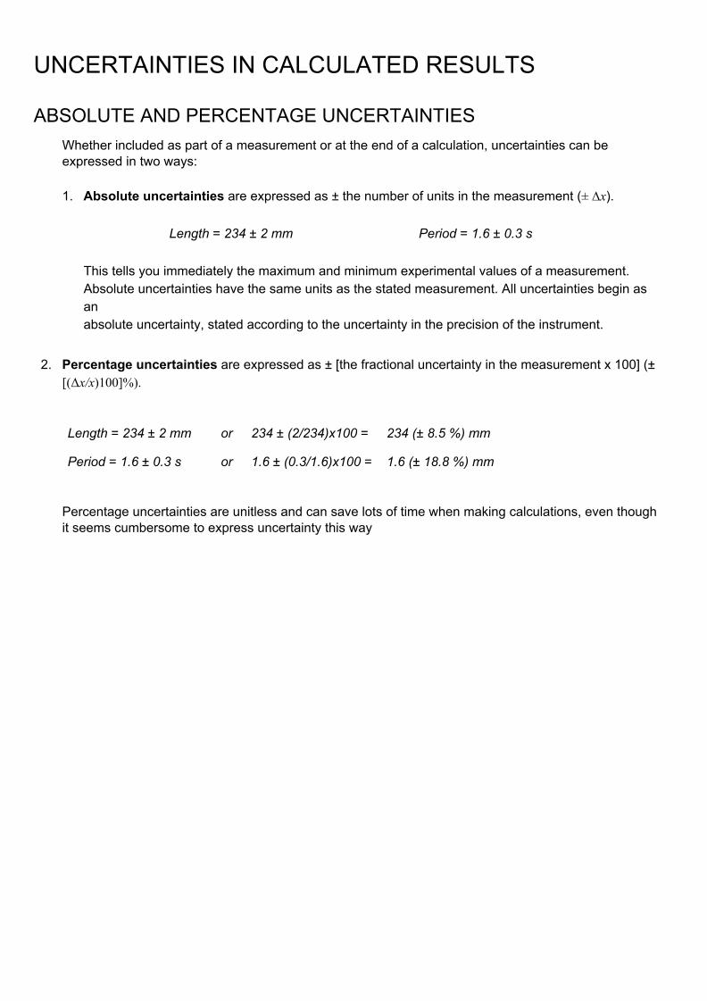
ABSOLUTE AND PERCENTAGE UNCERTAINTIES Whether included as part of a measurement or at the end of a calculation, uncertainties can be expressed in two ways:

1. Absolute uncertainties are expressed as ± the number of units in the measurement (± Δx).

Length = 234 ± 2 mm Period = 1.6 ± 0.3 s

This tells you immediately the maximum and minimum experimental values of a measurement. Absolute uncertainties have the same units as the stated measurement. All uncertainties begin as an absolute uncertainty, stated according to the uncertainty in the precision of the instrument.

2. Percentage uncertainties are expressed as ± [the fractional uncertainty in the measurement x 100] (± [(Δx/x)100]%).

Length = 234 ± 2 mm or 234 ± (2/234)x100 = 234 (± 8.5 %) mm

Period = 1.6 ± 0.3 s or 1.6 ± (0.3/1.6)x100 = 1.6 (± 18.8 %) mm

Percentage uncertainties are unitless and can save lots of time when making calculations, even though it seems cumbersome to express uncertainty this way

DETERMINING FINAL UNCERTAINTIES IN STATED RESULTS Physics is an experimental science, so we need to be concerned with how we treat uncertainties in calculated values using experimental data. The general rules are:

It is good form to leave all final calculated answers with an absolute uncertainty. Therefore, you need to be able to convert from absolute uncertainties to percentage and back again. Constants such as π do not affect the uncertainty calculation. When doing calculations involving percentage uncertainties, it is easier to leave out the (x 100) step and simply multiply using the decimal form

A cylinder has a radius of 1.60 ± 0.01 cm and a height of 11.5 ± 0.1 cm. Find the volume.

V = π r2 h = π (1.60)2 x 11.5 = 92.488 cm2 = 92 cm2

The percentage uncertainty in the radius is (0.01/1.60) x 100 = 0.625% (but leave as 0.00625). The percentage uncertainty in r2 is thus 2 x 0.00625 = 0.01250 The percentage uncertainty in the height is (0.1/11.5 0) x 100 = 0.87% (but leave as 0.00870).

So, the percentage uncertainty in the volume is 0.01250 + 0.00870 since we are multiplying h and r2.

= 0.02120 And the absolute uncertainty in V is 0.02120 x 92.488 cm2 = 1.96075 cm2

The final answer, with sig figs, is therefore V = 92 ± 2 cm2

Calculate the perimeter of a square that has a side of length 42±6mm

P = 4 d = 4 x 42 = 168 mm

The percentage uncertainty in the side length is (6/42) x 100 = 14.29% The percentage uncertainty in the multiplier ‘4’ = 0 % We are multiply d by 4 so the percentage uncertainty of 4d is equal to the sum of the percentage uncertainties of 4 and d.

% uncertainty of 4d = 0% + 14.29% = 14.29%

So the percentage of uncertainty of the perimeter is also 14.29% (because P=4d) So the absolute uncertainty is 14.29% of 168 mm = 24 mm

Therefore P = 168 ± 24 cm2

But we must round appropriately to get a final answer of P = 170 ± 30 cm2

cont...

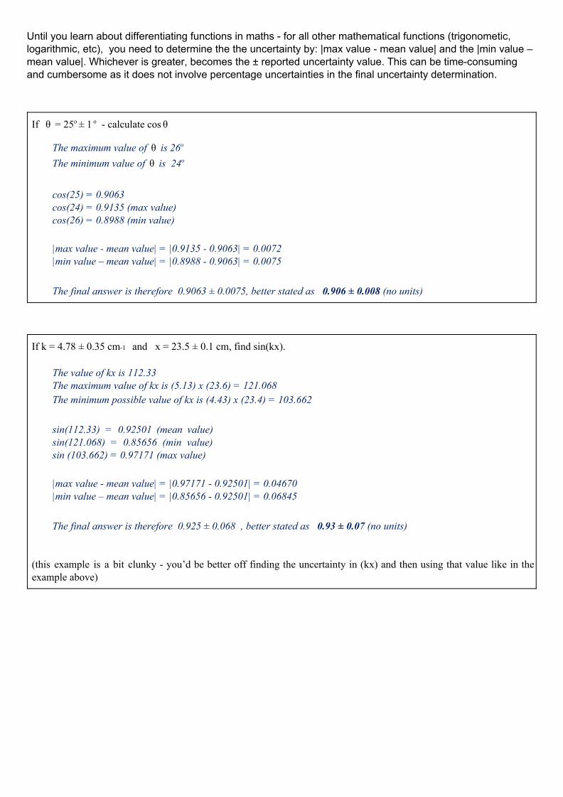
Until you learn about differentiating functions in maths - for all other mathematical functions (trigonometic, logarithmic, etc), you need to determine the the uncertainty by: |max value - mean value| and the |min value – mean value|. Whichever is greater, becomes the ± reported uncertainty value. This can be time-consuming and cumbersome as it does not involve percentage uncertainties in the final uncertainty determination.

If = 25o o - calculate cos θ ± 1 θ

The maximum value of is 26o θ

The minimum value of is 24o θ

cos(25) = 0.9063 cos(24) = 0.9135 (max value) cos(26) = 0.8988 (min value)

|max value - mean value| = |0.9135 - 0.9063| = 0.0072 |min value – mean value| = |0.8988 - 0.9063| = 0.0075

The final answer is therefore 0.9063 ± 0.0075, better stated as 0.906 ± 0.008 (no units)

If k = 4.78 ± 0.35 cm-1 and x = 23.5 ± 0.1 cm, find sin(kx).

The value of kx is 112.33 The maximum value of kx is (5.13) x (23.6) = 121.068 The minimum possible value of kx is (4.43) x (23.4) = 103.662

sin(112.33) = 0.92501 (mean value) sin(121.068) = 0.85656 (min value) sin (103.662) = 0.97171 (max value)

|max value - mean value| = |0.97171 - 0.92501| = 0.04670 |min value – mean value| = |0.85656 - 0.92501| = 0.06845

The final answer is therefore 0.925 ± 0.068 , better stated as 0.93 ± 0.07 (no units)

(this example is a bit clunky - you’d be better off finding the uncertainty in (kx) and then using that value like in the example above)

GRAPHICAL ANALYSIS Often, the point of a scientific experiment is to try and find empirical values for one or more physical quantities, given measurements of some other quantities and some mathematical relationship between them. For instance, given a marble has a mass of 5 g, and a radius of 0.7 cm, the density of the marble can be calculated given that V = 4/3πr3 and ρ = m/V. (For the sake of simplicity, uncertainties will be ignored for now). http://denethor.wlu.ca/data/linear.pdf

Many times, however, rather than having one measurement of a quantity, or set of quantities, we may have several measurements which should all follow the same relationships, (such as if we had several marbles made of the same material in the example above), and we wish to combine the results. The usual way of combining results is to create a graph, and extract information (such as the density) from the slope and y–intercept of the graph.

One may be tempted to ask why a graph should be better than merely averaging all of the data points. The answer is that an average is completely unbiased. The variation of any one point from the norm is no more or less important than the variation of any other point. A graph, however, will show any point which differs significantly from the general trend. Analysis of the graphical data (such as with a least squares fit) will allow such “outliers” to be given either more or less weight than the rest of the data as the researcher deems appropriate. Depending on the situation, the researcher may wish to verify any odd point(s), or perhaps the trend will indicate that a linear model is insufficient. In any case, it is this added interpretive value that a graph has which makes it preferable.

A plot is better than an average since it may indicate systematic errors in the data

The value in fitting the data to an equation is that once the fit has been done, rather than continuing to work with a large amount of data, we can simply work with the parameters of our fit and their uncertainties. In the case of a straight line, all of our data can be replaced by four quantities; the slope, the y-intercept and the uncertainties in both of these.

A fit equation replaces a bunch of data with a few parameters.

Humans are extremely good at processing information when it is presented visually. Scientists exploit this ability by presenting data in graphical form. Graphs can provide an excellent summary of many of the key features of an experiment. One of the most important types of graph is the x-y graph or scatterplot. Scientists are often interested in discovering whether there is a relationship between two variables, and scatterplots are ideal for displaying data relating to two variables.

X-Y SCATTERPLOTS An x-y scatterplot can indicate:

the range of measurements made the uncertainty of each measurement the existence of absence of a trend in the data the presence or absence of outliers (data points that do not follow the general trend)

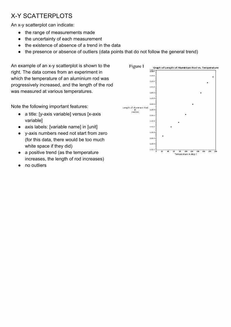
An example of an x-y scatterplot is shown to the right. The data comes from an experiment in which the temperature of an aluminium rod was progressively increased, and the length of the rod was measured at various temperatures. Note the following important features:

a title: [y-axis variable] versus [x-axis variable]

axis labels: [variable name] in [unit] y-axis numbers need not start from zero

(for this data, there would be too much white space if they did)

a positive trend (as the temperature increases, the length of rod increases)

no outliers

DEPENDENT AND INDEPENDENT VARIABLES One important question with x-y scatterplots is which variable to put on the x-axis and which to put on the y-axis. There is an agreed procedure for this, based on the distinction between independent and dependent variables. The variable that is controlled or deliberately altered by the experimenters is called the independent variable. This variable is usually plotted on the x-axis. The variable that varies in response to changes in the independent variable is called the dependent variable (because its values depend on the values of the independent variable). This variable is usually plotted on the y-axis. Note that in the graph title, the dependent variable is always written first. In the aluminium rod experiment it is the temperature that is varied by the experimenter. Hence temperature goes on the x-axis. The length of the rod varies in response to the changes in temperature (it ‘depends’ on the temperature). So rod length goes on the y-axis.

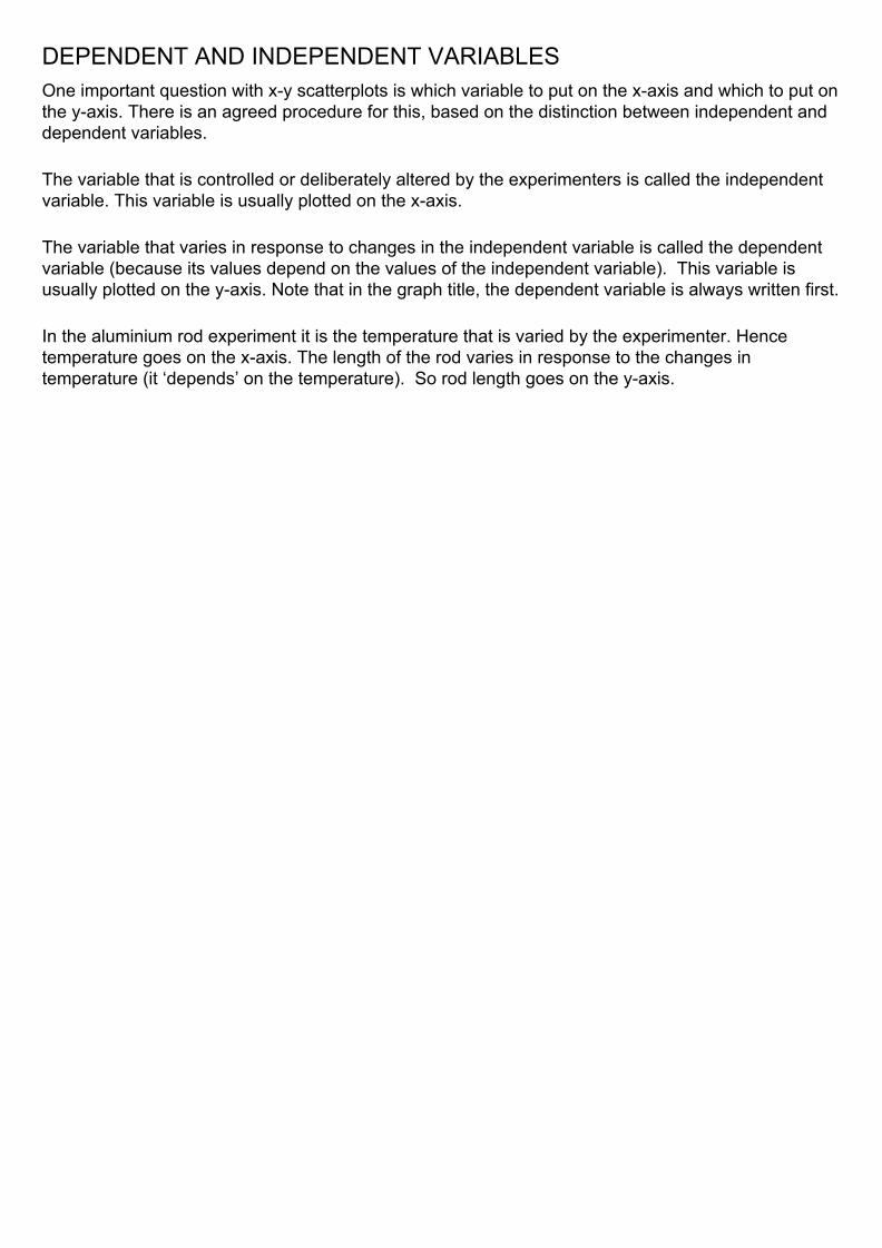
LINE OF BEST FIT When there appears to be a linear relationship between the independent and dependent variables (i.e. the data points tend to form a straight line), an important procedure is to draw in a line of best fit. A simple method for drawing a line of best fit ‘by eye’ is to use a transparent plastic ruler. The ruler should be positioned so that the data points appear to be scattered as evenly as possible above and below the line. Note that the point (0, 0) – the ‘origin’ – is not a special point, and the line of best fit should not be forced to go through it. (This is a much debated issue, and you may read differently elsewhere.) The graph below shows a line of best fit for the aluminium rod data:

Note the following points about a line of best fit:

roughly half the data points are above the line, and half below it it need not pass through any data points it replaces the individual data points for any further calculations it can be used to make predictions for values between the data points, and (less reliably) even

beyond the data point range

GRADIENT

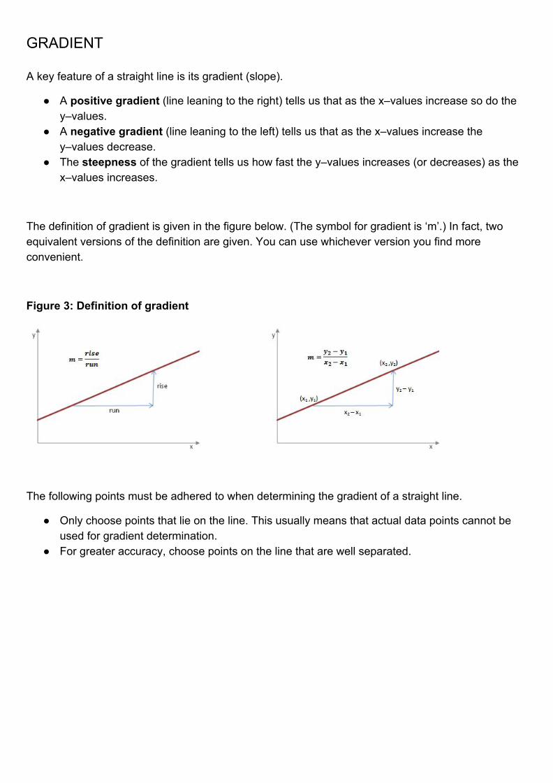
A key feature of a straight line is its gradient (slope).

A positive gradient (line leaning to the right) tells us that as the x–values increase so do the y–values.

A negative gradient (line leaning to the left) tells us that as the x–values increase the y–values decrease.

The steepness of the gradient tells us how fast the y–values increases (or decreases) as the x–values increases.

The definition of gradient is given in the figure below. (The symbol for gradient is ‘m’.) In fact, two equivalent versions of the definition are given. You can use whichever version you find more convenient.

Figure 3: Definition of gradient

The following points must be adhered to when determining the gradient of a straight line.

Only choose points that lie on the line. This usually means that actual data points cannot be used for gradient determination.

For greater accuracy, choose points on the line that are well separated.

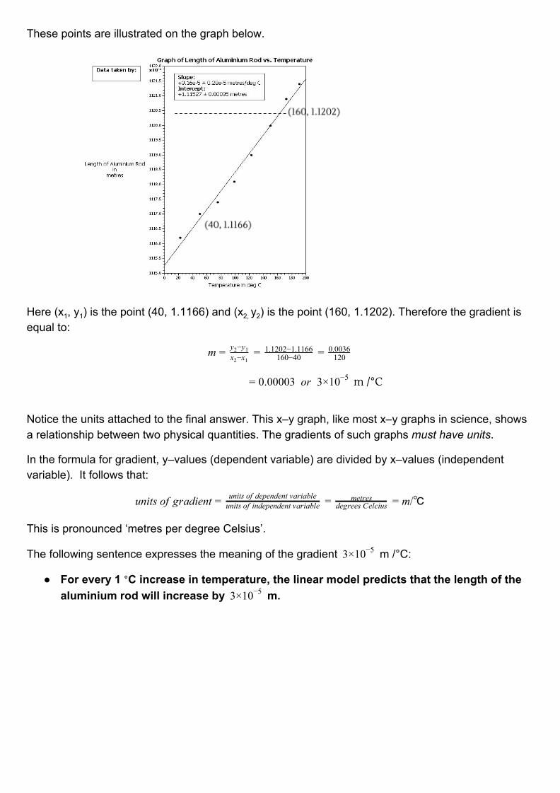
These points are illustrated on the graph below.

Here (x1, y1) is the point (40, 1.1166) and (x2, y2) is the point (160, 1.1202). Therefore the gradient is equal to:

m = x −x2 1

y −y2 1 = 160−401.1202−1.1166 = 120

0.0036

m /°C.00003 or 3×10= 0 −5

Notice the units attached to the final answer. This x–y graph, like most x–y graphs in science, shows a relationship between two physical quantities. The gradients of such graphs must have units.

In the formula for gradient, y–values (dependent variable) are divided by x–values (independent variable). It follows that:

nits of gradientu = units of dependent variableunits of independent variable = metres

degrees Celcius /= m

This is pronounced ‘metres per degree Celsius’.

The following sentence expresses the meaning of the gradient m /°C:×103 −5

For every 1 °C increase in temperature, the linear model predicts that the length of the aluminium rod will increase by m.×103 −5

EQUATION OF A STRAIGHT LINE

All straight lines have equations of the following form:

x y = m + c

where ‘m’ is the gradient, and ‘c’ is the y–intercept (the point where the line cuts the y–axis).

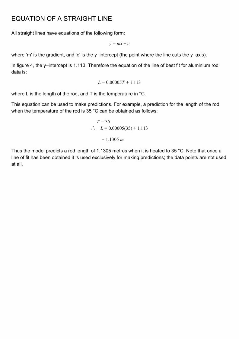
In figure 4, the y–intercept is 1.113. Therefore the equation of the line of best fit for aluminium rod data is:

.00005T .113 L = 0 + 1

where L is the length of the rod, and T is the temperature in °C.

This equation can be used to make predictions. For example, a prediction for the length of the rod when the temperature of the rod is 35 °C can be obtained as follows:

5T = 3 L .00005(35) .113 ∴ = 0 + 1

.1305 m = 1

Thus the model predicts a rod length of 1.1305 metres when it is heated to 35 °C. Note that once a line of fit has been obtained it is used exclusively for making predictions; the data points are not used at all.

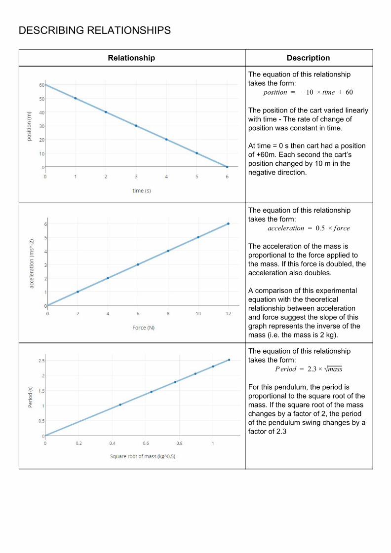
DESCRIBING RELATIONSHIPS

Relationship Description

The equation of this relationship takes the form:

osition 0 ime 60 p = − 1 × t + The position of the cart varied linearly with time - The rate of change of position was constant in time. At time = 0 s then cart had a position of +60m. Each second the cart’s position changed by 10 m in the negative direction.

The equation of this relationship takes the form:

cceleration 0.5 orce a = × f The acceleration of the mass is proportional to the force applied to the mass. If this force is doubled, the acceleration also doubles. A comparison of this experimental equation with the theoretical relationship between acceleration and force suggest the slope of this graph represents the inverse of the mass (i.e. the mass is 2 kg).

The equation of this relationship takes the form:

eriod 2.3 P = × √mass For this pendulum, the period is proportional to the square root of the mass. If the square root of the mass changes by a factor of 2, the period of the pendulum swing changes by a factor of 2.3

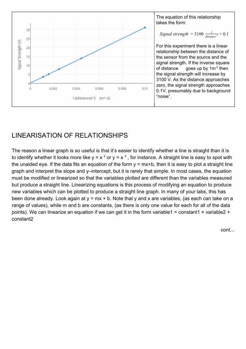
The equation of this relationship takes the form:

ignal strength 100 .1S = 3 1distance 2

+ 0

For this experiment there is a linear relationship between the distance of the sensor from the source and the signal strength. If the inverse square of distance goes up by 1m-2 then the signal strength will increase by 3100 V. As the distance approaches zero, the signal strength approaches 0.1V, presumably due to background “noise”.

LINEARISATION OF RELATIONSHIPS

The reason a linear graph is so useful is that it’s easier to identify whether a line is straight than it is to identify whether it looks more like y = x 2 or y = x 3 , for instance. A straight line is easy to spot with the unaided eye. If the data fits an equation of the form y = mx+b, then it is easy to plot a straight line graph and interpret the slope and y–intercept, but it is rarely that simple. In most cases, the equation must be modified or linearized so that the variables plotted are different than the variables measured but produce a straight line. Linearizing equations is this process of modifying an equation to produce new variables which can be plotted to produce a straight line graph. In many of your labs, this has been done already. Look again at y = mx + b. Note that y and x are variables, (as each can take on a range of values), while m and b are constants, (as there is only one value for each for all of the data points). We can linearize an equation if we can get it in the form variable1 = constant1 × variable2 + constant2

cont...

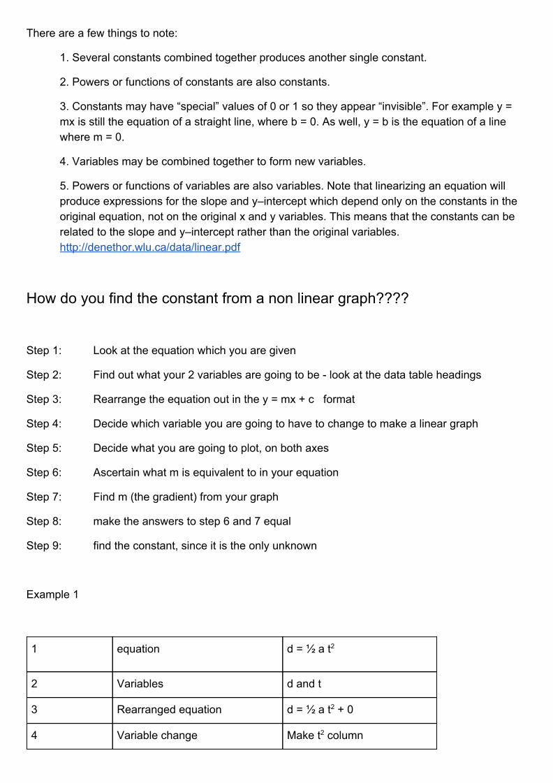
There are a few things to note:

1. Several constants combined together produces another single constant.

2. Powers or functions of constants are also constants.

3. Constants may have “special” values of 0 or 1 so they appear “invisible”. For example y = mx is still the equation of a straight line, where b = 0. As well, y = b is the equation of a line where m = 0.

4. Variables may be combined together to form new variables.

5. Powers or functions of variables are also variables. Note that linearizing an equation will produce expressions for the slope and y–intercept which depend only on the constants in the original equation, not on the original x and y variables. This means that the constants can be related to the slope and y–intercept rather than the original variables. http://denethor.wlu.ca/data/linear.pdf

How do you find the constant from a non linear graph????

Step 1: Look at the equation which you are given

Step 2: Find out what your 2 variables are going to be - look at the data table headings

Step 3: Rearrange the equation out in the y = mx + c format

Step 4: Decide which variable you are going to have to change to make a linear graph

Step 5: Decide what you are going to plot, on both axes

Step 6: Ascertain what m is equivalent to in your equation

Step 7: Find m (the gradient) from your graph

Step 8: make the answers to step 6 and 7 equal

Step 9: find the constant, since it is the only unknown

Example 1

1 equation d = ½ a t2

2 Variables d and t

3 Rearranged equation d = ½ a t2 + 0

4 Variable change Make t2 column

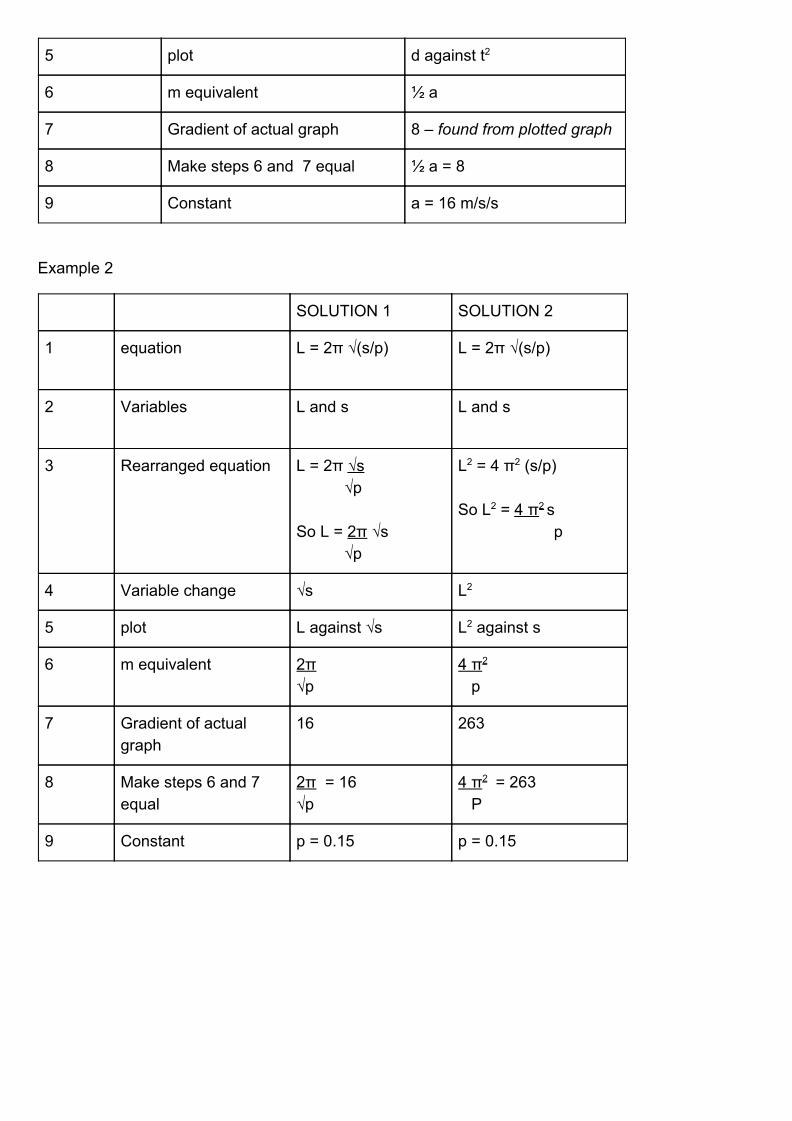
5 plot d against t2

6 m equivalent ½ a

7 Gradient of actual graph 8 – found from plotted graph

8 Make steps 6 and 7 equal ½ a = 8

9 Constant a = 16 m/s/s

Example 2

SOLUTION 1 SOLUTION 2

1 equation L = 2π √(s/p)

L = 2π √(s/p)

2 Variables L and s

L and s

3 Rearranged equation L = 2π √s √p So L = 2π √s √p

L2 = 4 π2 (s/p) So L2 = 4 π2 s p

4 Variable change √s L2

5 plot L against √s L2 against s

6 m equivalent 2π √p

4 π2

p

7 Gradient of actual graph

16 263

8 Make steps 6 and 7 equal

2π = 16 √p

4 π2 = 263 P

9 Constant p = 0.15 p = 0.15

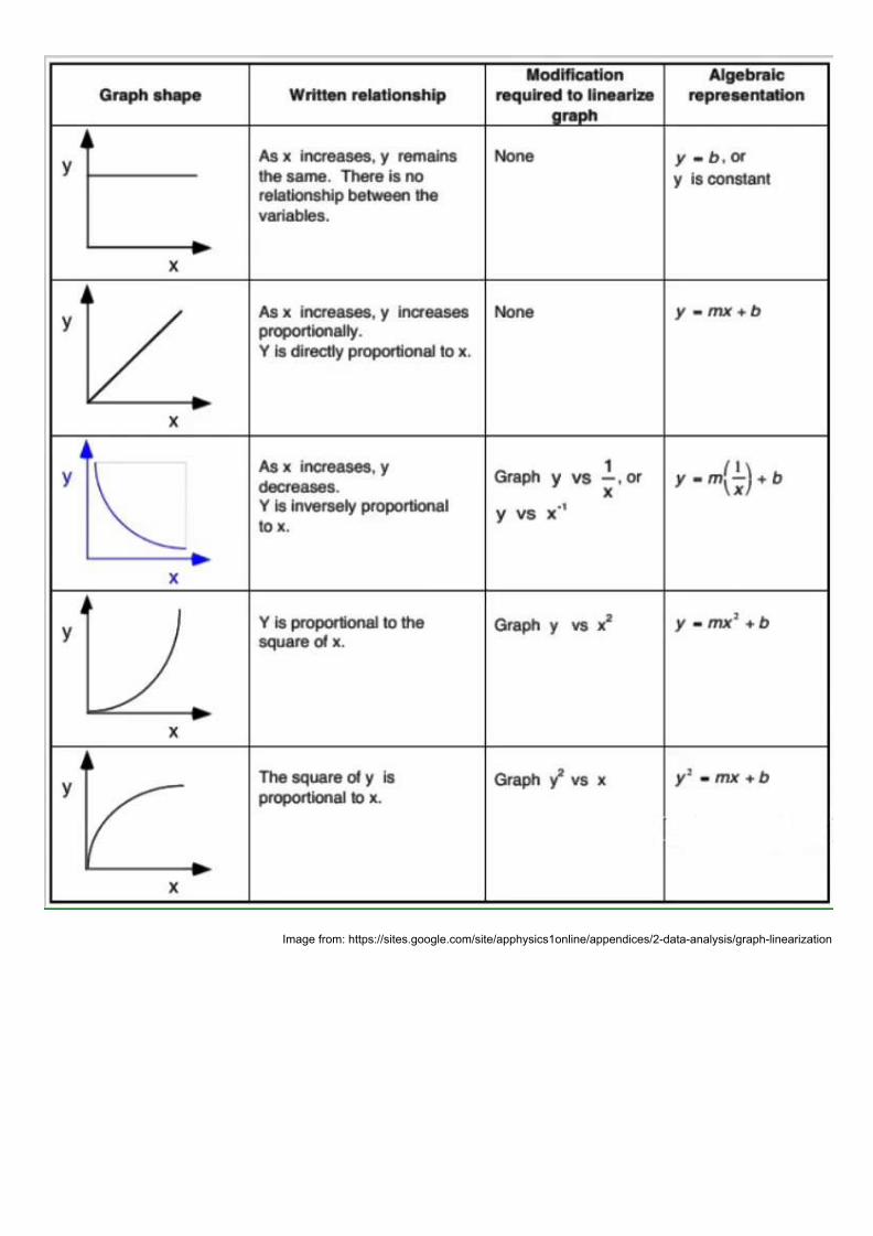
Image from: https://sites.google.com/site/apphysics1online/appendices/2-data-analysis/graph-linearization

STRUCTURE OF A PRACTICAL REPORT

RESEARCH QUESTION This will be a question that includes both the independent and dependent variables. The hypothesis is a possible answer to this question, and the actual answer should be in your conclusion.

BACKGROUND Many of the investigative procedures you do involve complicated concepts. Include here any information that helps the reader understand what you wanted to accomplish, and why. Research is needed to do a good job but put all information in your own words (read, take brief notes, put texts away, write it up). Use citations for key concepts and anything you didn’t already know. If appropriate include other experiments and their results done on this subject. Here would also be an appropriate place to state your general aim. You MUST reference all material with citations in this section.

HYPOTHESIS Predict an outcome based upon the background information. The quality of the hypothesis however, is crucial. Whatever you decide to try to prove, you must be sure that it has a relevant focus that matches the experiment. The independent and dependent variables should be identified in the hypothesis as well as the problem question. The usual format is “IF …something is done and it affects the object, THEN…..” Include a rationale or reason for your hypothesis which ties into your background.

VARIABLES A valuable way to make sure you include all your variables appropriately is to list and describe all your variables before you do the experiment.

Independent Variable: factor(s) that you are manipulating in your experiment. You are testing its effect on something. You should try to have only one independent variable so that you know that is the variable causing the change.

Dependent Variable: quantities you are measuring to determine if there is an effect from the independent variable. You do not manipulate the dependent variable directly. You are changing the independent variable and seeing if the dependent variable changes because is "depends" on the independent variable. Controlled Variables: quantities that need to be held the same in each trial to ensure a fair test. Note that controlled variables should be things that have values - e.g. room temperature is a controlled variable and it is kept constant by doing the experiment in the same room, on the same day. Items of equipment are NOT controlled variables.

EQUIPMENT All equipment used in the lab should be listed including sizes and quantities of each. Diagrams of experiment set-up are appropriate; but do not include pictures of individual pieces of equipment.

METHOD A description of the procedure used to carry out the experiment should be clear enough for anyone else to follow and reproduce your experiment in detail. If you use a specialised apparatus, include a labeled diagram or photo. You may also include a table of how your trials will be set up if it makes your procedure more clear. As well as the basic steps, specify all the techniques you use to maximise your accuracy and precision, with brief justification.

RAW DATA The actual data measured during the investigation. Include any qualitative data. For all data tables, include a descriptive caption which outlines the details of that particular experiment and any additional comments that might be appropriate. Make sure tables contain a caption, symbols and units for each column, columns for any calculations you will have to do and the appropriate number of significant digits. Include the uncertainty of the individual data points at the top of each column of measurement or in a separate column. If appropriate, add justification for uncertainty estimates in the table caption.

DATA PROCESSING When looking at the effect of one variable on another, you will need to do some calculations and graph your data to look at the relationship between the variables. The graph can also tell you a lot about the experimental errors that might be affecting your results. Keep the following tips in mind when presenting your processed data:

For all calculation types, including uncertainties, include an explanation or annotated example. Uncertainties in any data also need to be propagated through calculations. Graphs must include descriptive caption that outlines the details of the experiment(s) Graphs should also include units, error bars, have an appropriate scale Non-linear relationships should be linearised if possible.

CONCLUSION AND EVALUATION

This is the most important part of an experiment - it is where you look at your data and interpret what it is telling you. The evaluation should be part of the experiment cycle - to improve your processes. Take into account the following questions when writing your conclusion and evaluation. They do not have to be in any particular order.

Explain what the results tell you - What is the answer to your research question?

Restate the hypothesis and compare your conclusion to it.

Do the data follow current scientific trends, or were there errors that leave your conclusion questionable?

Compare your results/values with the literature. Any comparison must take uncertainties into account. Use citations when you read other sources and included their ideas.

How reliable are your results? You must take into account any systematic or random errors and uncertainties.

What story is your data telling you? - Were the measurements accurate (close to the true values) and precise (close to each

other)? - Look at your graph - compare the scatter of the data to the error bars - Is the slope and y-intercept what you expected - if not, what errors might be influencing the

results? - What does your data tell you about random and/or systematic uncertainty?

What weaknesses were there in the design and method of your investigation?

Discuss any difficulties.

The impact of errors and suggestions for improvement should also be included. Be quantitative in your discussion of the impact of the errors.

How could you have performed this lab better?

What use is doing this lab and how might the data be used?

Are there further experiments that can be performed or did the data suggest other avenues to explore?

What anomalies were there and where were the errors? How did those affect the data?

cont...

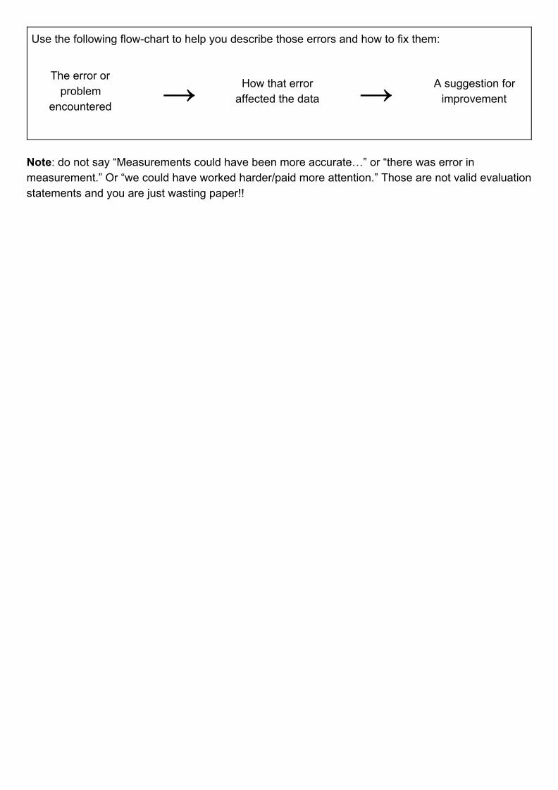
Use the following flow-chart to help you describe those errors and how to fix them:

The error or problem

encountered → How that error affected the data → A suggestion for

improvement

Note: do not say “Measurements could have been more accurate…” or “there was error in measurement.” Or “we could have worked harder/paid more attention.” Those are not valid evaluation statements and you are just wasting paper!!

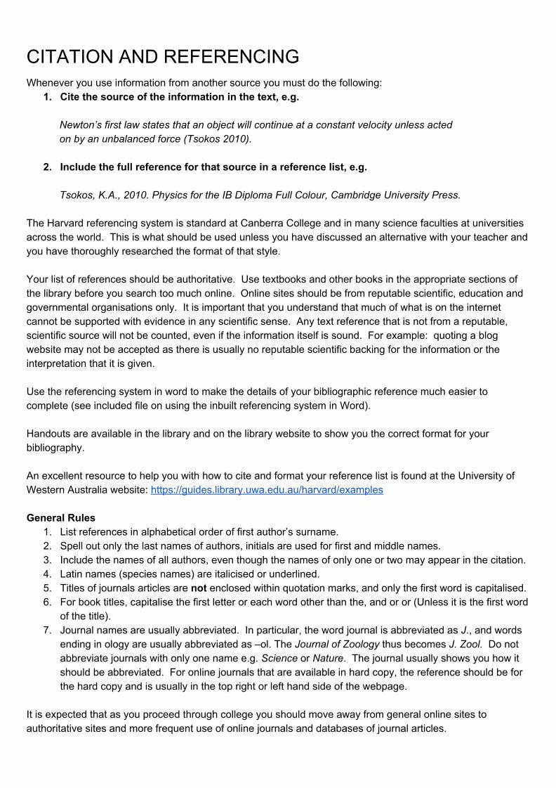
CITATION AND REFERENCING Whenever you use information from another source you must do the following:

1. Cite the source of the information in the text, e.g.

Newton’s first law states that an object will continue at a constant velocity unless acted on by an unbalanced force (Tsokos 2010).

2. Include the full reference for that source in a reference list, e.g.

Tsokos, K.A., 2010. Physics for the IB Diploma Full Colour, Cambridge University Press.

The Harvard referencing system is standard at Canberra College and in many science faculties at universities across the world. This is what should be used unless you have discussed an alternative with your teacher and you have thoroughly researched the format of that style. Your list of references should be authoritative. Use textbooks and other books in the appropriate sections of the library before you search too much online. Online sites should be from reputable scientific, education and governmental organisations only. It is important that you understand that much of what is on the internet cannot be supported with evidence in any scientific sense. Any text reference that is not from a reputable, scientific source will not be counted, even if the information itself is sound. For example: quoting a blog website may not be accepted as there is usually no reputable scientific backing for the information or the interpretation that it is given. Use the referencing system in word to make the details of your bibliographic reference much easier to complete (see included file on using the inbuilt referencing system in Word). Handouts are available in the library and on the library website to show you the correct format for your bibliography. An excellent resource to help you with how to cite and format your reference list is found at the University of Western Australia website: https://guides.library.uwa.edu.au/harvard/examples General Rules

1. List references in alphabetical order of first author’s surname. 2. Spell out only the last names of authors, initials are used for first and middle names. 3. Include the names of all authors, even though the names of only one or two may appear in the citation. 4. Latin names (species names) are italicised or underlined. 5. Titles of journals articles are not enclosed within quotation marks, and only the first word is capitalised. 6. For book titles, capitalise the first letter or each word other than the, and or or (Unless it is the first word

of the title). 7. Journal names are usually abbreviated. In particular, the word journal is abbreviated as J., and words

ending in ology are usually abbreviated as –ol. The Journal of Zoology thus becomes J. Zool. Do not abbreviate journals with only one name e.g. Science or Nature. The journal usually shows you how it should be abbreviated. For online journals that are available in hard copy, the reference should be for the hard copy and is usually in the top right or left hand side of the webpage.

It is expected that as you proceed through college you should move away from general online sites to authoritative sites and more frequent use of online journals and databases of journal articles.

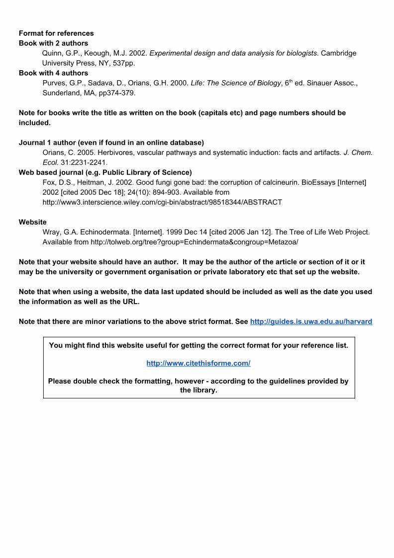
Format for references Book with 2 authors

Quinn, G.P., Keough, M.J. 2002. Experimental design and data analysis for biologists. Cambridge University Press, NY, 537pp.

Book with 4 authors Purves, G.P., Sadava, D., Orians, G.H. 2000. Life: The Science of Biology, 6th ed. Sinauer Assoc., Sunderland, MA, pp374-379.

Note for books write the title as written on the book (capitals etc) and page numbers should be included. Journal 1 author (even if found in an online database)

Orians, C. 2005. Herbivores, vascular pathways and systematic induction: facts and artifacts. J. Chem. Ecol. 31:2231-2241.

Web based journal (e.g. Public Library of Science) Fox, D.S., Heitman, J. 2002. Good fungi gone bad: the corruption of calcineurin. BioEssays [Internet] 2002 [cited 2005 Dec 18]; 24(10): 894-903. Available from http://www3.interscience.wiley.com/cgi-bin/abstract/98518344/ABSTRACT

Website

Wray, G.A. Echinodermata. [Internet]. 1999 Dec 14 [cited 2006 Jan 12]. The Tree of Life Web Project. Available from http://tolweb.org/tree?group=Echindermata&congroup=Metazoa/

Note that your website should have an author. It may be the author of the article or section of it or it may be the university or government organisation or private laboratory etc that set up the website. Note that when using a website, the data last updated should be included as well as the date you used the information as well as the URL. Note that there are minor variations to the above strict format. See http://guides.is.uwa.edu.au/harvard

You might find this website useful for getting the correct format for your reference list.

http://www.citethisforme.com/

Please double check the formatting, however - according to the guidelines provided by the library.