photometry and spectroscopy of the new sdbv cs 1246

arX

iv:0

912.

3903

v1 [

astr

o-ph

.SR

] 1

9 D

ec 2

009

Mon. Not. R. Astron. Soc. 000, 000–000 (0000) Printed 19 December 2009 (MN LATEX style file v2.2)

Photometry and spectroscopy of the new sdBV CS 1246⋆

B.N. Barlow12†, B.H. Dunlap12, J.C. Clemens1, A.E. Lynas-Gray3,

K.M. Ivarsen1, A.P. LaCluyze1, D.E. Reichart1, J.B. Haislip1 & M.C. Nysewander4

1Department of Physics and Astronomy, University of North Carolina, Chapel Hill, NC 27599-3255, USA2Visiting astronomer, CTIO, NOAO, which is operated by the AURA, under contract with the NSF.3Department of Physics, University of Oxford, Keble Road, Oxford OX1 3RH, England4Alion Science & Technology, 1000 Park Forty Plaza, Durham, NC 27713, USA

19 December 2009

ABSTRACT

We report the discovery of a large-amplitude oscillation in the hot subdwarf B star CS1246 and present multi-colour photometry and time-resolved spectroscopy supportingthis discovery. We used the 0.41-m PROMPT array to acquire data in the u’, g’, r’, andi’ filters simultaneously over 3 consecutive nights in 2009 April. These data reveal asingle oscillation mode with a period of 371.707 ± 0.002 s and an amplitude dependentupon wavelength, with a value of 34.5 ± 1.6 mma in the u’ filter. We detected noadditional frequencies in any of the light curves. Subsequently, we used the 4.1-mSOAR telescope to acquire a time-series of 248 low-resolution spectra spanning 6 hrsto look for line profile variations. Models fits to the spectra give mean atmosphericvalues of Teff = 28450 ± 700 K and log g = 5.46 ± 0.11 undergoing variations withsemi-amplitudes of 507 ± 55 K and 0.034 ± 0.009, respectively. We also detect aradial velocity oscillation with an amplitude of 8.8 ± 1.1 km s−1. The relationshipbetween the angular and physical radii variations shows the oscillation is consistentwith a radial mode. Under the assumption of a radial pulsation, we compute the stellardistance, radius, and mass as d = 460 ± 190

90pc, R = 0.19 ± 0.08 R⊙, and M = 0.39

±0.300.13 M⊙, respectively, using the Baade-Wesselink method.

Key words: stars: individual: CS 1246 – stars: oscillations – subdwarfs

1 INTRODUCTION

Hot subdwarf B (sdB) stars are evolved objects presumed tohave He-burning cores and modelled as extended horizontalbranch stars (Heber 1986). They dominate surveys of faintblue objects and are often cited as the main source of theUV-upturn observed in globular clusters and giant ellipticalgalaxies. Their temperatures range from 20000 to 40000 K,and their log g values span more than an order of magnitudefrom 5 to 6.2. Their evolutionary histories are not entirelyunderstood; various formation scenarios are possible includ-ing both single-star and binary-star channels (D’Cruz et al.1996; Han et al. 2002, 2003). At least two thirds of themappear to be in binary systems (Saffer et al. 2001; Maxtedet al. 2001), but a higher binary fraction cannot be ruledout. Han et al. (2002, 2003) have even shown it is possibleto explain 100% of the sdB stars as the products of binary-star channels. In either case, sdB stars probably evolve fromthe red giant branch after losing a signficant portion of theirouter H envelopes, and stellar models show they will evolve

† E-mail:[email protected]

directly to the white dwarf cooling sequence after exhaust-ing the He in their cores (Dorman et al. 1993). Their opticalspectra are dominated by H Balmer lines and sometimes alsodisplay He I or even the 4686 A He II line. See Heber (2009)for a review on what is currently known about sdB stars.

More than a decade ago, Kilkenny et al. (1997) re-ported the first detection of photometric oscillations in a sdBstar (EC 14026-2647). Contemporaneous with this discov-ery, Charpinet et al. (1996, 1997) predicted the existence ofa class of sdB pulsators after calculating stellar models thatshowed driving of p-modes. The oscillations they found weredriven by the κ-mechanism and associated with an opacitybump from the ionisation of Fe in their model envelopes.The discovery of the first pulsator sparked an interest insdB variability studies, and, subsequently, around 70 pul-sators have been discovered to date. Many techniques havebeen applied to sdB pulsators successfully including multi-colour photometry (see Tremblay et al. 2006 for a summary)and time-resolved spectroscopy (pioneered by O’Toole et al.2000; Telting & Østensen 2004; Tillich et al. 2007). Astero-seismological studies of these stars have revealed informationabout their internal structure, including total mass, envelope

http://arxiv.org/abs/0912.3903v1

2 Barlow et al.

mass, and chemical stratification and have been carried outon a handful of sdB pulsators (see Brassard et al. 2001 andCharpinet et al. 2005 as examples). Østensen (2009) presentsa thorough review of asteroseismolgy and its successes.

Observationally, the subdwarf B pulsators may be di-vided into three classes: the rapid (sdBVr), slow (sdBVs),and hybrid (sdBVrs) pulsators1. The sdBVr stars are as-sociated with models of p-mode pulsators and have periodsbetween 80 and 600 s and typical amplitudes less than 1%.In the log g-Teff plane, they cluster together in an insta-bility strip with Teff ranging from 28000 to 35000 K andlog g between 5.2 and 6.1. The sdBVs stars generally haveperiods from 1 to 2 hrs with amplitudes of only a few tenthsof a percent; their oscillations are modelled with g modes.They are also found in an instability strip with Teff be-tween 23000 and 30000 K and log g near 5.4. In the regionwhere the blue edge of the sdBVs instability strip overlapsthe red edge of the sdBVr strip, three sdBVrs stars havebeen observed with fast and slow oscillations (Schuh et al.2006; Baran et al. 2006; Lutz et al. 2009). Both of the in-stability strips contain stars that have been observed not tovary photometrically.

The most fundamental parameters of any star, the massand radius, are not well known for sdB stars and are rarelycomputed from observations. Single and binary evolutioncalculations point to a canonical mass of 0.47 M⊙ (Han et al.2002, 2003), and a few masses supporting this result havebeen derived from asteroseismology (e.g., Brassard et al.2001; Randall et al. 2007) and from eclipsing binaries (e.g.,Wood et al. 1993, Drechsel et al. 2001). Zhang et al. (2009)have even proposed a new technique for deriving statisticalmasses from observational data in the literature. Most of thesdB radii measurements to date come from binary systemsfor which the separation distance is known; the sdB radiusis derived from the ratio of the radii and assumes informa-tion about the companion. Such studies show a typical sdBradius to be near 0.2 R⊙, but additional and more directmeasurements are needed to confirm this result.

We report the detection of a single, large-amplitude os-cillation in the sdB star CS 1246 (α2000=12:49:37.69, δ2000=-63:32:08.99), an object first observed by Reid et al. (1988)in a survey of hot white dwarfs and OB subdwarfs in ob-scured regions of the Galactic plane. In one of the mostopaque sections of the Coalsack Dark Nebula, CS 1246 wasidentified by Reid et al. (1988) as a candidate hot subdwarfB star with a V magnitude of 14.59 ± 0.14 and U-B andB-V colours of -1.08 ± 0.10 and 0.28 ± 0.10, respectively.Neither Teff nor log g has previously been determined.

We first learned of CS 1246 while browsing the on-line Subdwarf Database (Østensen 2006) for candidate pul-sators observable with the 0.41-m Panchromatic RoboticOptical Monitoring and Polarimetry Telescopes (PROMPT)in Chile. Even though there were no available estimates ofTeff or log g, we decided to look for pulsations since theU-B colour roughly matched that of known pulsators and

1 Here we adopt the naming scheme in which all sdB pulsatorsare given the base name ’sdBV’; subscripts ’r’ and ’s’ are addedupon observations of rapid and slow oscillations, respectively. Forreference, the sdBVr stars are also called V361 Hya and EC 14026stars, while the sdBVs stars have the aliases PG 1716, V1093 Her,and ’Betsy’ stars.

the star was a brighter, Southern-hemisphere target. Thediscovery run data revealed an interesting light curve, andwe subsequently obtained multi-colour time-series photome-try and time-resolved spectroscopy to study the pulsations.We observed line profile variations in the spectra and foundsubstantial oscillations in the radial velocity, temperature,and gravity. The nature of these variations is consistent withthat expected for an ℓ = 0 pulsation, but we cannot rule outthe possibility of non-radial modes with our current dataset. Although not one of our original goals, we were able tocompute the distance, radius, and mass of CS 1246 from therelation between the physical and angular radii variations.Our study is the first to apply such a method to an sdBVstar, and the results show the mass and radius to be con-sistent with those calculated for other sdB stars in binariesand from theory.

2 DISCOVERY OF THE PULSATION

We first observed CS 1246 on 2009 March 30 after sub-mitting a job to the PROMPT queue using the web-basedSKYNET interface (see §3.1 for a description of these sys-tems). Later that night PROMPT 4 monitored the star forapproximately 75 min, obtaining an uninterrupted series of80 exposures through a Johnson V filter with integrationtimes of 40 s and a duty cycle of 89%. Even before removingatmospheric extinction effects or transparency variations, werealized CS 1246 was a pulsator as its oscillations were visi-ble in the undivided, raw light curve. After formally reducingand analysing the data using the methods described in §3.2and §3.3, we found a single oscillation with a period of 372s and an amplitude of 23 mma. Figure 1 shows the reducedlight curve and its amplitude spectrum. No other frequencieswere observed in this data set, which had a mean noise levelof 1.6 mma. The relatively long period and large amplitudeof the oscillation inspired us to obtain simultaneous multi-colour photometry with the PROMPT and time-resolvedspectroscopy with the SOAR telescope. These observationsand the results thereof are described in the sections thatfollow.

3 MULTI-COLOUR PHOTOMETRY

3.1 The instrument

PROMPT is a system of 0.41-m Ritchey-Chretien telescopesat Cerro Tololo Inter-American Observatory (CTIO) inChile built primarily for rapid and simultaneous multiwave-length observations of gamma-ray burst afterglows. Table 1presents some of the CCD characteristics of these telescopes.The PROMPT telescopes are 100% automated and operateunder the control of SKYNET, a prioritised queue schedul-ing system that allows registered users to acquire, view, anddownload data from any location via a PHP-enabled Webserver. Observations in the queue are assigned priority lev-els and scheduled accordingly; gamma-ray bursts receive toppriority. The SKYNET system enables automated data col-lection at times that would be inconvenient or impossible fora human observer. For example, our multi-colour photomet-ric programme was executed by PROMPT while BNB andBHD were in Detroit, Michigan, supporting the University of

Photometry and spectroscopy of CS 1246 3

0 1000 2000 3000 4000Time (s)

-50

0

50

Am

plitu

de (

mm

a)

0 2000 4000 6000 8000Frequency (µHz)

0

10

20

Am

plitu

de (

mm

a)

Figure 1. Light curve (upper panel) and amplitude spectrum(lower panel) of the discovery run data from 2009 March 30. Thelight curve was produced from V-filtered data and is presentedunsmoothed.

Table 1. Characteristics of the PROMPT CCDs

Telescope Size Pixel Scale Gain Readnoise(pix) (arcsec/pix) (e−/ADU) (e−)

PROMPT 2 3k x 2k 0.41 1.6 8.3PROMPT 3 1k x 1k 0.59 1.6 8.3PROMPT 4 1k x 1k 0.59 1.4 7.6PROMPT 5 1k x 1k 0.59 1.4 9.2

North Carolina Men’s Basketball team at the 2009 NCAANational Championship. Obtaining the data presented in§3.2 using classical observing methods would have been anexpensive and time-consuming undertaking. For additionaldetails on PROMPT and SKYNET, refer to Reichart et al.(2005).

N

E

1 arcmin

C1

C2

C3

C4

C5

C6C7

C8

C9

Figure 2. CS 1246 field. Image shown is a stack of 30 40-s V-bandframes taken with PROMPT 4. CS 1246 is indicated with a starwhile the comparison stars are marked with circles and labeledC1-C9.

3.2 Observations and reductions

PROMPT obtained multi-colour photometry simultane-ously through the u’, g’, r’, and i’ filters on 2009 April 4,5, and 6 using all available telescopes. Table 2 presents adetailed log of these observations. The CCD parameters ofthe PROMPT telescopes (Table 1) and SKYNET overheadresulted in duty cycles of 94%, 80%, 89%, and 89% for theu’, g’, r’, and i’ filter data sets, respectively, during the con-tinuous portions of the runs. Although the majority of theruns were uninterrupted, each data set contains an approx-imately 15-minute long gap due to the inability of the eq-uitorial mounts to track through the meridian. Additional40-minute gaps are present in the u’ and g’ data from 2009April 6. In total, our 3-day photometry campaign produced113 hours of data with 7291 useable frames.

After bias-subtracting, dark-subtracting, and flat-fielding the frames with IRAF using conventional proce-dures, we extracted our photometry using the external IRAFpackage CCD HSP written by Antonio Kanaan. Apertureradii were chosen to maximize the signal-to-noise (S/N) ra-tio in the light curves and were always less than the seeingwidth. We used sky annuli to subtract the sky counts fromeach stellar aperture, being sure to avoid contamination ofthe annuli with other stars in the field. We divided the sky-subtracted light curves by an average of constant comparisonstar light curves to correct for transparency variations; thesestars are labeled in the field image shown in Figure 2. Someof them lacked an adequate S/N ratio through some filterswhile saturating the CCD in others, and, consequently, weemployed different comparison stars for different filters (seeTable 2). We are confident that the results of our frequencyanalyses are independent of the choices of the comparisonstars, as they all appeared to be constant. Atmospheric ex-tinction effects were approximated and removed each nightby fitting and normalising the curves with parabolas. Weused the WQED suite (Thompson & Mullally 2009) to ana-lyze the data and apply timing corrections to the barycentreof the solar system. Figure 3 presents the full, differentially-corrected light curves.

3.3 Frequency analysis

We analysed our reduced light curves using two tools: thediscrete Fourier transform and the least-squares fitting ofsine waves. WQED, again, was used to access these tools.Figure 4a presents the amplitude spectra for the combinedlight curves shown in Figure 3 along with their window func-tions. The u’ and g’ amplitude spectra are plotted out totheir respective Nyquist frequencies, while the r’ and i’ spec-tra are terminated at 10 mHz (beyond this point these spec-tra are consistent with noise).

Inspection of the amplitude spectra reveals a single,dominant mode at 2690.29 µHz (371.707s) with amplitudesof 32.0 ± 1.5, 24.4 ± 0.9, 21.3 ± 0.3, and 20.6 ± 0.4 mmain the u’, g’, r’, and i’ passbands, respectively. Table 3 sum-marizes the results of the least-squares fits; the errors shownare derived directly from the fits and assume uncorrelatednoise. The results of Montgomery & O’Donoghue (1999) im-ply these errors may be larger by a factor of three. We detectno phase differences between the four colour curves withinour level of precision. As the integration times of our expo-

4 Barlow et al.

Table 2. Multicolour photometry observations log

Start Timea Date Filter Telescope Texp Tcycle Length # Frames Comparison Stars(UT) (UT) (s) (s) (hrs)

23:59:02.8 2009 Apr 04 u’ PROMPT 3 80 86 9.4 393 C1,C2,C900:57:03.3 2009 Apr 05 g’ PROMPT 2 40 52 8.7 592 C1,C2,C3,C4,C8,C900:01:47.7 2009 Apr 05 r’ PROMPT 4 40 47 9.6 710 C2,C3,C4,C5,C700:01:51.7 2009 Apr 05 i’ PROMPT 5 40 47 9.6 710 C2,C3,C4,C5,C6



aTime at midpoint of first exposure.

-0.1

0.0

0.1

Fra

ctio

nal A

mpl

itude

u’

-0.1

0.0

0.1

g’

-0.1

0.0

0.1

r’

0 50000 100000 150000 200000Time Since BJED 2454925.50315492 (s)

-0.1

0.0

0.1

i’

22000 24000 26000

Figure 3. Light curves of CS 1246 over 3 consecutive nights (left panels) taken simultaneously through the u’, g’, r’, and i’ filters (fromtop to bottom). These observations represent a total of 113 hours of data taken with 7291 frames. Expanded views (right panels) of thesame 1.5-hour section of the curves are shown to illustrate the variable nature of the star.

sures are significant fractions of the 371.7-s period, we musttake phase smearing into account. For any measured observ-able oscillating with a period P and a physical amplitude A,a finite integration time I will result in a reduced observedamplitude Ao given by

Ao =P

πIsin(

πI

P)A, (1)

Baldry (1999) presents a discussion of phase smearing and aderivation of this equation. The amplitudes we measure forthe 371.7-s variation underestimate the physical amplitudesby 7.4% in the u’ filter and 1.9% in the g’, r’, and i’ filters.The smearing-corrected amplitudes are 34.5 ± 1.6, 24.8 ±

0.9, 21.7 ± 0.3, and 21.0 ± 0.4 mma in the u’, g’, r’, and i’filters, respectively.

After fitting the dominant mode and subtracting the fitfrom the light curves, we recalculated the Fourier transformsof the residual light curves; they are shown in Figure 4b. Themean noise levels in these pre-whitened u’, g’, r’, and i’ am-plitude spectra are 1.9, 1.1, 0.3, and 0.5 mma, respectively.All of the spectra show a heightened noise level at extremelylow frequencies, but this is likely a side effect of our methodfor extinction removal. Beyond the low-frequency regime,some of the pre-whitened spectra show peaks at or above the3-σ level. However, none of these periodicities were detectedin more than one data set, whether from night-to-night orfrom filter-to-filter, so we evaluate their signficance using


(a)

0.000.01

0.02

0.03

Fra

ctio

nal A

mpl

itude

u’

0.00

0.01

0.02g’

0.00

0.01

0.02

r’

0 2000 4000 6000 8000 Frequency (µHz)

0.00

0.01

0.02

i’

-200 -100 0 100 200Frequency (µHz)

(b)

0.000

0.005

0.010

Fra

ctio

nal A

mpl

itude

u’

0.000

0.003

0.006 g’

0.000

0.001

r’

0 2000 4000 6000 8000 10000Frequency (µHz)

0.0000.001

0.002

i’

Figure 4. Amplitude spectra of the combined light curves in the u’, g’, r’, and i’ filters (from top to bottom) before (a) and after (b)pre-whitening of the main mode. The window functions for each data set are shown in the right portion of (a). In the pre-whitenedspectra, the 3σ and 4σ levels are represented by dashed and dot-dashed lines, respectively, and the position of the pre-whitened signalis marked with a vertical dashed line. The u’ and g’ spectra are plotted out to their respective Nyquist frequencies. The r’ and i’ plotsare terminated at 10 mHz but are consistent with noise beyond this point.

the false alarm probability (Horne & Baliunas 1986). Noneof them meet our significance test of a false alarm probabil-ity <1%. Moreover, the folded pulse shapes agree with thatof a single sinusoid to within the errors, implying a lack ofharmonically-related frequencies in the light curve.

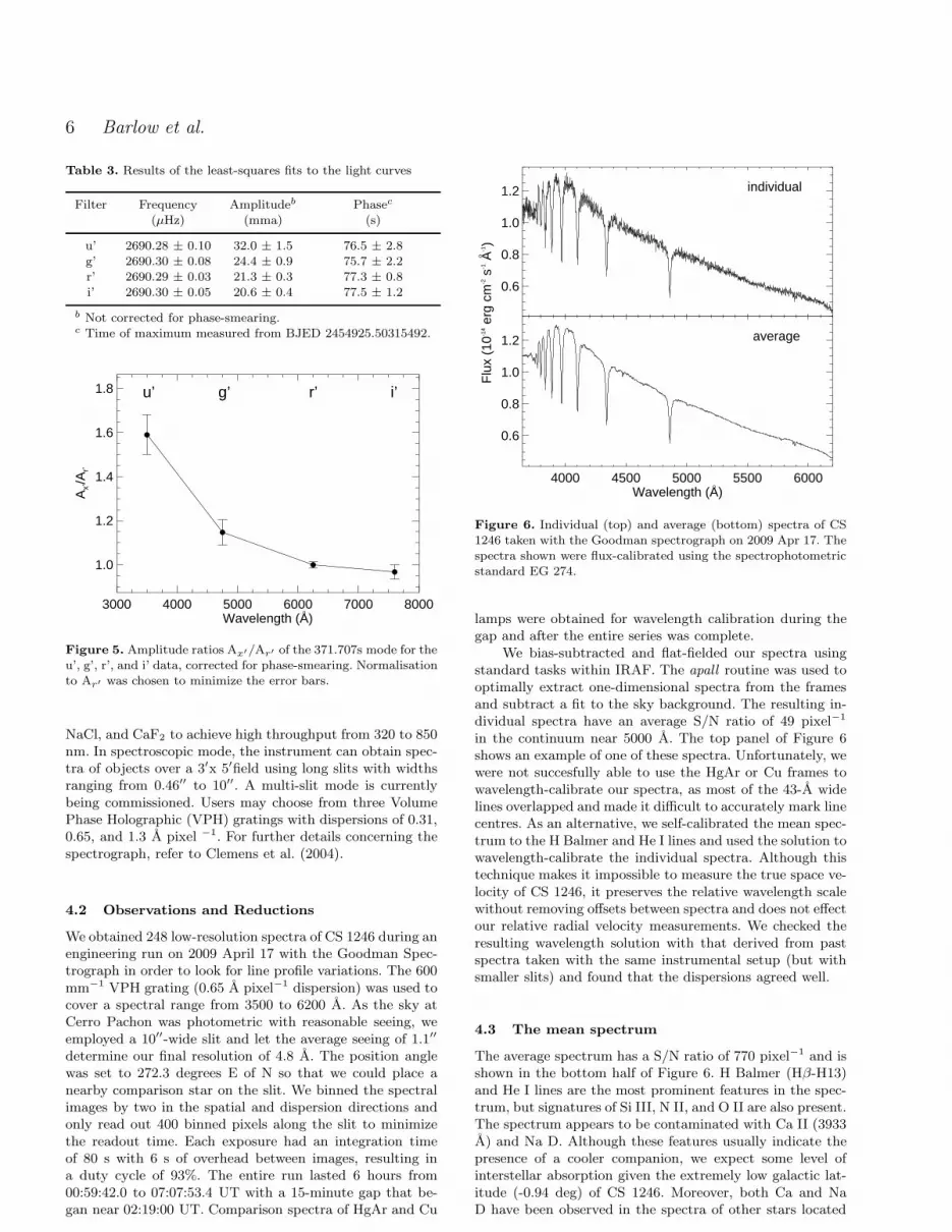
The amplitude of the oscillation is strongly wavelength-dependent, as illustrated in Figure 5. The u’ amplitude is thelargest, being 39%, 59%, and 64% greater than those in theg’, r’, and i’ filters, respectively. In principle, these ratios maybe used along with the known atmospheric parameters of thestar to estimate the degree l of the oscillation, but in ourcase the large error bars make such an exercise inconclusive.

4 TIME-RESOLVED SPECTROSCOPY

4.1 The instrument

The Goodman Spectrograph is an imaging spectrographbuilt for one of the Nasmyth ports of the 4.1-m SOARtelescope on Cerro Pachon in Chile. In imaging mode, thecamera-collimator combination re-images the SOAR focalplane with a focal reduction of three times, yielding a platescale of 0.15 arcsec pixel−1 at the CCD. The camera con-tains a 4k x 4k Fairchild 486 back-illuminated CCD withelectronics and dewar provided by Spectral Instruments, Inc.of Tucson, Arizona. The system uses optics of fused silica,

6 Barlow et al.

Table 3. Results of the least-squares fits to the light curves

Filter Frequency Amplitudeb Phasec

(µHz) (mma) (s)

u’ 2690.28 ± 0.10 32.0 ± 1.5 76.5 ± 2.8g’ 2690.30 ± 0.08 24.4 ± 0.9 75.7 ± 2.2r’ 2690.29 ± 0.03 21.3 ± 0.3 77.3 ± 0.8i’ 2690.30 ± 0.05 20.6 ± 0.4 77.5 ± 1.2

b Not corrected for phase-smearing.c Time of maximum measured from BJED 2454925.50315492.

3000 4000 5000 6000 7000 8000Wavelength (A)

1.0

1.2

1.4

1.6

1.8

Ax’/A

r’

u’ g’ r’ i’

o

Figure 5. Amplitude ratios Ax′/Ar′ of the 371.707s mode for theu’, g’, r’, and i’ data, corrected for phase-smearing. Normalisationto Ar′ was chosen to minimize the error bars.

NaCl, and CaF2 to achieve high throughput from 320 to 850nm. In spectroscopic mode, the instrument can obtain spec-tra of objects over a 3′x 5′field using long slits with widthsranging from 0.46′′ to 10′′. A multi-slit mode is currentlybeing commissioned. Users may choose from three VolumePhase Holographic (VPH) gratings with dispersions of 0.31,0.65, and 1.3 A pixel −1. For further details concerning thespectrograph, refer to Clemens et al. (2004).

4.2 Observations and Reductions

We obtained 248 low-resolution spectra of CS 1246 during anengineering run on 2009 April 17 with the Goodman Spec-trograph in order to look for line profile variations. The 600mm−1 VPH grating (0.65 A pixel−1 dispersion) was used tocover a spectral range from 3500 to 6200 A. As the sky atCerro Pachon was photometric with reasonable seeing, weemployed a 10′′-wide slit and let the average seeing of 1.1′′

determine our final resolution of 4.8 A. The position anglewas set to 272.3 degrees E of N so that we could place anearby comparison star on the slit. We binned the spectralimages by two in the spatial and dispersion directions andonly read out 400 binned pixels along the slit to minimizethe readout time. Each exposure had an integration timeof 80 s with 6 s of overhead between images, resulting ina duty cycle of 93%. The entire run lasted 6 hours from00:59:42.0 to 07:07:53.4 UT with a 15-minute gap that be-gan near 02:19:00 UT. Comparison spectra of HgAr and Cu

0.6

0.8

1.0

1.2

Flu

x (1

0-14 e

rg c

m-2 s

-1 A

-1)

individual

o4000 4500 5000 5500 6000

Wavelength (A)

0.6

0.8

1.0

1.2 average

o

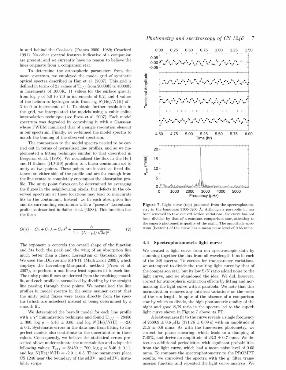
Figure 6. Individual (top) and average (bottom) spectra of CS1246 taken with the Goodman spectrograph on 2009 Apr 17. Thespectra shown were flux-calibrated using the spectrophotometricstandard EG 274.

lamps were obtained for wavelength calibration during thegap and after the entire series was complete.

We bias-subtracted and flat-fielded our spectra usingstandard tasks within IRAF. The apall routine was used tooptimally extract one-dimensional spectra from the framesand subtract a fit to the sky background. The resulting in-dividual spectra have an average S/N ratio of 49 pixel−1

in the continuum near 5000 A. The top panel of Figure 6shows an example of one of these spectra. Unfortunately, wewere not succesfully able to use the HgAr or Cu frames towavelength-calibrate our spectra, as most of the 43-A widelines overlapped and made it difficult to accurately mark linecentres. As an alternative, we self-calibrated the mean spec-trum to the H Balmer and He I lines and used the solution towavelength-calibrate the individual spectra. Although thistechnique makes it impossible to measure the true space ve-locity of CS 1246, it preserves the relative wavelength scalewithout removing offsets between spectra and does not effectour relative radial velocity measurements. We checked theresulting wavelength solution with that derived from pastspectra taken with the same instrumental setup (but withsmaller slits) and found that the dispersions agreed well.

4.3 The mean spectrum

The average spectrum has a S/N ratio of 770 pixel−1 and isshown in the bottom half of Figure 6. H Balmer (Hβ-H13)and He I lines are the most prominent features in the spec-trum, but signatures of Si III, N II, and O II are also present.The spectrum appears to be contaminated with Ca II (3933A) and Na D. Although these features usually indicate thepresence of a cooler companion, we expect some level ofinterstellar absorption given the extremely low galactic lat-itude (-0.94 deg) of CS 1246. Moreover, both Ca and NaD have been observed in the spectra of other stars located


in and behind the Coalsack (Franco 2000, 1989; Crawford1991). No other spectral features indicative of a companionare present, and we currently have no reason to believe thelines originate from a companion star.

To determine the atmospheric parameters from themean spectrum, we employed the model grid of syntheticoptical spectra described in Han et al. (2007). This grid isdefined in terms of 21 values of Teff from 20000K to 40000Kin increments of 1000K, 11 values for the surface gravityfrom log g of 5.0 to 7.0 in increments of 0.2, and 4 valuesof the helium-to-hydrogen ratio from log N (He)/N (H) of -3 to 0 in increments of 1. To obtain further resolution inthe grid, we interpolated the models using a cubic splineinterpolation technique (see Press et al. 2007). Each modelspectrum was degraded by convolving it with a Gaussianwhose FWHM mimicked that of a single resolution elementin our spectrum. Finally, we re-binned the model spectra tomatch the binning of the observed spectrum.

The comparison to the model spectra needed to be car-ried out in terms of normalised line profiles, and so we im-plemented a fitting technique similar to that described inBergeron et al. (1995). We normalised the flux in the He Iand H Balmer (Hβ-H9) profiles to a linear continuum set tounity at two points. These points are located at fixed dis-tances on either side of the profile and are far enough fromthe line centre to completely encompass the absorption pro-file. The unity point fluxes can be determined by averagingthe fluxes in the neighbouring pixels, but defects in the ob-served spectrum at these locations may lead to inaccuratefits to the continuum. Instead, we fit each absorption lineand its surrounding continuum with a “pseudo” Lorentzianprofile as described in Saffer et al. (1988). This function hasthe form

G(λ) = C0 + C1λ + C2λ2 +

A

1 + [(λ − µ)/√

2σ]α. (2)

The exponent α controls the overall shape of the functionand fits both the peak and the wing of an absorption linemuch better than a classic Lorenztian or Gaussian profile.We used the IDL routine MPFIT (Markwardt 2009), whichemploys the Levenberg-Marquardt method (Press et al.2007), to perform a non-linear least-squares fit to each line.The unity point fluxes are derived from the resulting smoothfit, and each profile is normalised by dividing by the straightline passing through these points. We normalised the lineprofiles in model spectra in the same manner except thatthe unity point fluxes were taken directly from the spec-tra (which are noiseless) instead of being determined by asmooth fit.

We determined the best-fit model for each line profilewith a χ2 minimization technique and found Teff = 28450± 300, log g = 5.46 ± 0.06, and log N (He)/N (H) = -2.0± 0.1. Systematic errors in the data and from fitting to im-perfect models also contribute to the uncertainties in thesevalues. Consequently, we believe the statistical errors pre-sented above underestimate the uncertainties and adopt thefollowing values: Teff = 28450 ± 700, log g = 5.46 ± 0.11,and log N (He)/N (H) = -2.0 ± 0.3. These parameters placeCS 1246 near the boundary of the sdBVr and sdBVs insta-bility strips.

-0.050.000.05

0.00 0.25 0.50 0.75 1.00 1.25 1.50

Fra

ctio

nal A

mpl

itude

4.50 4.75 5.00 5.25 5.50 5.75 6.00Time (hr)

0 1000 2000 3000 4000 5000Frequency (µHz)

0

5

10

15

20A

phot (

mm

a)

Figure 7. Light curve (top) produced from the spectrophotom-etry in the bandpass 3500-6200 A. Although a parabolic fit hasbeen removed to take out extinction variations, the curve has notbeen divided by that of a constant comparison star, attesting tothe superb photometric quality of the night. The amplitude spec-trum (bottom) of the curve has a mean noise level of 0.65 mma.

4.4 Spectrophotometric light curve

We created a light curve from our spectroscopic data bysumming together the flux from all wavelength bins in eachof the 248 spectra. To correct for transparency variations,we attempted to divide the resulting light curve by that ofthe comparison star, but its low S/N ratio added noise to thelight curve, and we abandoned the idea. We did, however,correct for atmospheric extinction effects by fitting and nor-malising the light curve with a parabola. We note that thisnormalisation removes any intrinsic variations on the orderof the run length. In spite of the absence of a comparisonstar by which to divide, the high photometric quality of thenight and good S/N ratio in the spectra led to the superblight curve shown in Figure 7 above its FT.

A least-squares fit to the curve reveals a single frequencyof 2689.9 ± 0.6 µHz (371.76 ± 0.09 s) with an amplitude of21.5 ± 0.6 mma. As with the time-series photometry, wecorrect for phase smearing, which leads to a damping of7.45%, and derive an amplitude of 23.3 ± 0.7 mma. We de-tect no additional periodicities with signficant probabilitiesfrom the light curve, which had a mean noise level of 0.65mma. To compare the spectrophotometry to the PROMPTresults, we convolved the spectra with the g’ filter trans-mission function and repeated the light curve analysis. We

8 Barlow et al.

0 1 2 3 4 5 6Time (hr)

-50

0

50OI

-50

0

50

V-V

(km

s-1)

Hβ

_

Figure 8. Radial velocities obtained from fitting pseudoLorentzian profiles to the stellar Hβ line (top) and the 5577 AO I sky emission line (bottom). The large-scale variation is dueto instrumental flexure.

find a smearing-corrected amplitude of 23.2 ± 0.7 mma inagreement with the g’ filter result from §3.3 .

4.5 Radial velocity curve

To construct a radial velocity curve, we individually fit theHβ-H9 profiles in each spectrum with ”pseudo” Lorentzianfunctions as described in §4.3, fixing the α parameter to thevalue determined from the average spectrum. The individualspectra did not have the S/N ratio needed to fit the otherabsorption line profiles accurately, and, consequently, theselines were ignored in our analysis. The locations of the profilecentres in the mean spectrum were subtracted from those inthe individual spectra, and the shifts from the mean wereconverted to km s−1.

The top panel in Figure 8 shows the resulting radial ve-locity curve for Hβ, as an example. The data exhibit a long-term variation spanning approximately 100 km s−1 over thecourse of the run. We attribute this structure to the com-bination of two factors: the global change in instrumentalflexure and the movement of the star at the focal plane. Asthe sky fills the entire slit, we may correct the former by ex-amining the drift of atmospheric emission lines. The latterproblem is more difficult to correct, and, consequently, wedo not attempt to do so. Previous time-series photometryruns with the Goodman Spectrograph, however, show thedrift due to guiding to be small, usually around 0.3′′ over atime span much longer than the period of CS 1246.

To compensate for flexure, we fit the O I sky line in eachspectrum with a Gaussian using the GAUSSFIT routine inIDL and obtained the curve shown in the bottom panel ofFigure 8. A 5th-order polynomial matched the O I curvefairly well, and we removed this trend from the velocitycurves of the stellar absorption lines. After flexure correc-tion, the velocity curves were linear with slopes dependentupon wavelength. This result is expected from atmosphericrefraction and allows us to approximate the guiding wave-length as 8400 A. We computed the global radial velocitycurve by removing the linear variations due to refraction

-250

25

0.00 0.25 0.50 0.75 1.00 1.25 1.50

V-V

(km

s-1)

_

4.50 4.75 5.00 5.25 5.50 5.75 6.00Time (hr)

0 1000 2000 3000 4000 5000Frequency (µHz)

0

2

4

6

8A

RV (

km s

-1)

Figure 9. Flexure-corrected radial velocity curve (top) producedfrom the weighted average of the Hβ-H9 velocity curves. The am-plitude spectrum (bottom) has a mean noise level of 0.94 km s−1.Shortcomings in our flexure-correction are visible in the 3.25-4.0hr section of the curve and give rise to the low-frequency peak inthe FT near 143 µHz.

and averaging the velocities from all of the H Balmer lines,weighting each curve by the inverse of its variance. Figure 9shows the resulting radial velocity curve along with its FT.

A strong radial velocity variation accompanies the pho-tometric oscillation at the same frequency. After barycen-tric correction of the velocities and the mid-exposure times,we find a semi-amplitude of 8.2 ± 1.0 km s−1 by fittinga sine curve with frequency fixed to that derived from thePROMPT data. Sine wave fits to the velocity curves of theindividual Hβ-H9 lines give amplitudes of 8.7, 7.2, 7.5, 8.6,8.9, and 9.8 km s−1, respectively. The uncertainty we re-port for the average velocity is the standard deviation ofthese values. The increase in velocity with increasing Balmerorder (with the exception of Hβ) implies the velocity iswavelength-dependent, as expected from weighting of theprojected velocities over the observed hemisphere by limb-darkening. Correcting for phase smearing, we derive a finalsemi-amplitude of 8.8 ± 1.1 km s−1. We claim no additionalcandidate frequencies after pre-whitening the data with themain pulsation period. The large peak in the FT near 143µHz is a result of an imperfect flexure correction and shouldnot be attributed to stellar oscillations. The mean noise levelin the amplitude spectrum is 0.94 km s−1.


4.6 Effective temperature and gravity variations

We determined Teff and log g as a function of pulsationphase by phase-folding and averaging the spectra togetherin 10 evenly-spaced bins. The resulting spectra had S/N ra-tios of approximately 240 pixel−1 in the continuum near5000 A. We fit atmospheric models to the spectra in themanner described in §4.3 to determine Teff , log g, andlog N (He)/N (H) over a pulsation cycle. As we observed nochange in the He abundance over the 10 phase bins, we fixedthe abundance to its average value and refit the other atmo-spheric parameters.

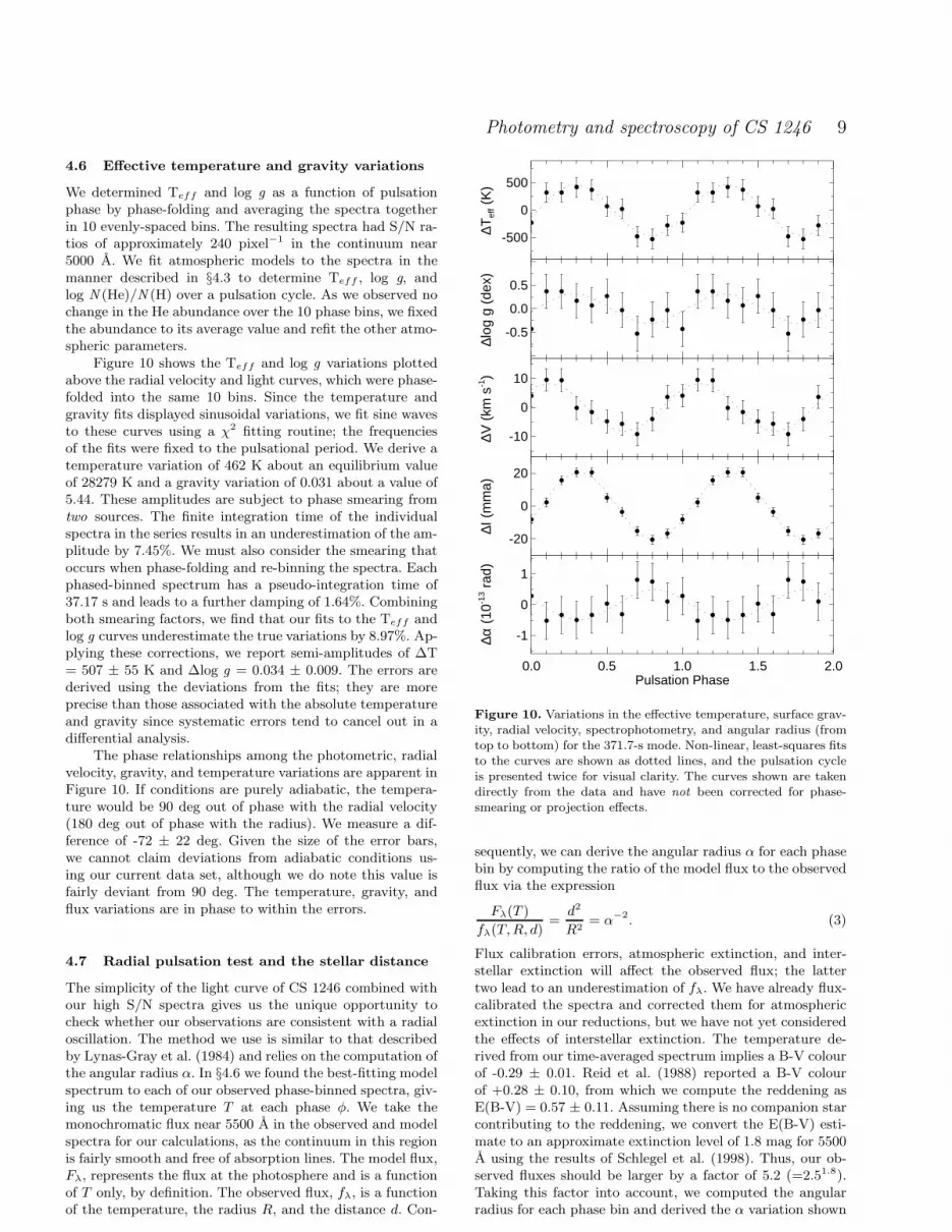
Figure 10 shows the Teff and log g variations plottedabove the radial velocity and light curves, which were phase-folded into the same 10 bins. Since the temperature andgravity fits displayed sinusoidal variations, we fit sine wavesto these curves using a χ2 fitting routine; the frequenciesof the fits were fixed to the pulsational period. We derive atemperature variation of 462 K about an equilibrium valueof 28279 K and a gravity variation of 0.031 about a value of5.44. These amplitudes are subject to phase smearing fromtwo sources. The finite integration time of the individualspectra in the series results in an underestimation of the am-plitude by 7.45%. We must also consider the smearing thatoccurs when phase-folding and re-binning the spectra. Eachphased-binned spectrum has a pseudo-integration time of37.17 s and leads to a further damping of 1.64%. Combiningboth smearing factors, we find that our fits to the Teff andlog g curves underestimate the true variations by 8.97%. Ap-plying these corrections, we report semi-amplitudes of ∆T= 507 ± 55 K and ∆log g = 0.034 ± 0.009. The errors arederived using the deviations from the fits; they are moreprecise than those associated with the absolute temperatureand gravity since systematic errors tend to cancel out in adifferential analysis.

The phase relationships among the photometric, radialvelocity, gravity, and temperature variations are apparent inFigure 10. If conditions are purely adiabatic, the tempera-ture would be 90 deg out of phase with the radial velocity(180 deg out of phase with the radius). We measure a dif-ference of -72 ± 22 deg. Given the size of the error bars,we cannot claim deviations from adiabatic conditions us-ing our current data set, although we do note this value isfairly deviant from 90 deg. The temperature, gravity, andflux variations are in phase to within the errors.

4.7 Radial pulsation test and the stellar distance

The simplicity of the light curve of CS 1246 combined withour high S/N spectra gives us the unique opportunity tocheck whether our observations are consistent with a radialoscillation. The method we use is similar to that describedby Lynas-Gray et al. (1984) and relies on the computation ofthe angular radius α. In §4.6 we found the best-fitting modelspectrum to each of our observed phase-binned spectra, giv-ing us the temperature T at each phase φ. We take themonochromatic flux near 5500 A in the observed and modelspectra for our calculations, as the continuum in this regionis fairly smooth and free of absorption lines. The model flux,Fλ, represents the flux at the photosphere and is a functionof T only, by definition. The observed flux, fλ, is a functionof the temperature, the radius R, and the distance d. Con-

-500

0

500

∆Tef

f (K

)

-0.5

0.0

0.5

∆log

g (

dex)

-10

0

10

∆V (

km s

-1)

-20

0

20∆I

(m

ma)

0.0 0.5 1.0 1.5 2.0Pulsation Phase

-1

0

1

∆α (

10-1

3 rad

)

Figure 10. Variations in the effective temperature, surface grav-ity, radial velocity, spectrophotometry, and angular radius (fromtop to bottom) for the 371.7-s mode. Non-linear, least-squares fitsto the curves are shown as dotted lines, and the pulsation cycleis presented twice for visual clarity. The curves shown are takendirectly from the data and have not been corrected for phase-smearing or projection effects.

sequently, we can derive the angular radius α for each phasebin by computing the ratio of the model flux to the observedflux via the expression

Fλ(T )

fλ(T, R, d)=

d2

R2= α−2. (3)

Flux calibration errors, atmospheric extinction, and inter-stellar extinction will affect the observed flux; the lattertwo lead to an underestimation of fλ. We have already flux-calibrated the spectra and corrected them for atmosphericextinction in our reductions, but we have not yet consideredthe effects of interstellar extinction. The temperature de-rived from our time-averaged spectrum implies a B-V colourof -0.29 ± 0.01. Reid et al. (1988) reported a B-V colourof +0.28 ± 0.10, from which we compute the reddening asE(B-V) = 0.57 ± 0.11. Assuming there is no companion starcontributing to the reddening, we convert the E(B-V) esti-mate to an approximate extinction level of 1.8 mag for 5500A using the results of Schlegel et al. (1998). Thus, our ob-served fluxes should be larger by a factor of 5.2 (=2.51.8).Taking this factor into account, we computed the angularradius for each phase bin and derived the α variation shown

10 Barlow et al.

in the bottom panel of Figure 10. A least-squares fit to thecurve gives a semi-amplitude of 4.88∗10−14 rad (5.36∗10−14

rad after smearing-correction) about a mean angular radiusof 1.01 ∗ 10−11 rad. We stress again that errors in the fluxcalibration and extinction estimates lead to incorrect valuesfor the angular radii and their relative differences.

A plot of ∆α vs ∆R will reveal a linear relationship fora radial pulsation mode, as shown by the relation

∆α =∆R

d, (4)

where the distance is the inverse of the slope. Having alreadyderived the α variations, we compute the variations in thephysical radius by integrating the radial velocity curve. Weconverted the observed expansion velocities into actual ex-pansion velocities using a projection factor dependent uponrelative limb darkening in the spectral lines. Montanes Ro-driguez & Jeffery (2001) computed such factors for early-type, radially pulsating stars, and their studies show a valueof 1.4 to be appropriate for an sdB star like CS 1246. Byapplying this factor, we assume from this point on that the371.7-s mode is radial in nature and can only check whetherour observations are consistent with this assumption. Thevelocity amplitude becomes 12.3 ± 1.4 km s−1 after applica-tion of the projection factor, and integration of this velocitygives a physical radius variation with semi-amplitude of 728± 83 km.

Figure 11 presents a plot of ∆α against ∆R. To test fora linear relationship, we computed the Pearson correlationcoefficient and find a value of 0.78. The probability that 10measurements of two uncorrelated variables can produce acorrelation coefficient at or above this value is less than 2%(see Appendix A). We can neither rule out the possibilitythat the 371.7-s mode in CS 1246 is a radial one, nor canwe exclude the possibility of a mode with ℓ > 0.

Still under the assumption of a radial mode, we fit a lineto the data and determined the distance from the slope viaEqn. 4. As ∆α = 0 should correspond to the point where ∆R= 0, we force the fit to pass through this point and derive adistance of d = 460 ± 190

100 pc. An sdB star this close should bebrighter than what Reid et al. (1988) measured. In fact, withTeff=28450±700 K and R=0.19±0.08 R⊙ (see §4.8), CS1246 should have an apparent Visual magnitude of 12.7±0.9

0.5

when observed at the above distance. This value implies aVisual extinction level of 1.9±1.0

0.6 mags, in agreement withthat found by Rodgers (1960) and Mattila (1970) for thepart of the Coalsack where CS 1246 resides.

4.8 The stellar radius and mass

We are now in the position to compute the radius and massdirectly from our observations using two different methods.The observed variations in log g come about from the pul-sational acceleration and changes in the radius, and afterthe former contribution is subtracted, the radius may bederived from the remaining difference. Unfortunately, theuncertainty in ∆log g yields excessively large error bars onour determination of the radius and, consequently, the mass,and for this reason we deem this method unreliable with ourcurrent data set. A second method proves to be more fruitfuland is based upon the Baade-Wesselink method. Any frac-tional change in the angular radius should yield the same

-1.0

-0.5

0.0

0.5

1.0

∆α (

10-1

3 rad

)

-0.001 0.000 0.001∆R (Rsun)

-1.0

0.0

1.0

Res

idua

ls

Figure 11. Plot of ∆α vs ∆R. For a radial pulsator, these vari-ables should exhibit a linear relationship. The dashed line denotesthe linear fit to these data. The data exhibit a Pearson correla-tion coefficient of 0.78. A representative error bar is shown forthe leftmost data point and was computed by propagating errorsthrough Eqn 3.

fractional change in the physical radius. Using this fact andlinearizing Eqn. 3, we compute R from the following relation:

∆R

R=

∆α

α=

1

2

„

∆fλ

fλ− ∆Fλ

Fλ

«

. (5)

This expression yields a radius of R = 0.19 ± 0.08 R⊙. Sim-ilar results are obtained by calculating the radius directlyfrom α and d, which gives R = 0.20 ±0.11

0.06 R⊙. We presentthe derivation of R using Eqn 5 to illustrate that errors in theobserved flux cancel out and do not affect the computationof the physical radius as they do the distance calculation.

Combined with our measurement of the mean surfacegravity, the radius derived from Eqn 5 gives a mass of M= 0.39 ±0.30

0.13 M⊙. Again, the radius and mass we reportare meaningless if the pulsation is non-radial. Although ourerrors bars are large, the mass agrees with the commonly-accepted value of 0.5 M⊙. The radius is also consistent withthose determined for other sdB stars from binary obser-vations and from theoretical mass-radius relationships buthas been computed using more direct observations. Work-ing backwards and assuming a canonical mass of 0.5 M⊙,we would derive a radius of R = 0.22 R⊙ from the mean logg value.

5 CONCLUSIONS

We report the discovery of an exciting new member of thesdBVr class of pulsators, CS 1246. Our simultaneous, multi-colour, time-series photometry reveals a single oscillationmode with period 371.7 s. The amplitude of this mode de-pends strongly on wavelength and is largest in the u’ filter.We detect no additional periodicities in the frequency spec-tra, although we note our 0.41-m telescope detection limits


are poor. The light curve of CS 1246 appears to be the sim-plest of all sdBV stars.

Time-series spectroscopy proved to be a much morefruitful exercise than we originally anticipated. We detectedvariations in temperature, gravity, and radial velocity atthe same frequency as the photometric oscillations. Inter-estingly, the ratios of these amplitudes (507 K, 0.034, 8.8km s−1) scale extremely well with those found by Østensenet al. (2007) for the main mode of Balloon 090100001 (1186K, 0.084, 18.9 km s−1), which Baran et al. (2008) have con-firmed as a radial oscillation. By comparing changes in theangular and physical radii, we have shown the pulsationmode in CS 1246 is consistent with a radial one, but wecannot rule out non-radial modes with our current data set.We were able, however, to calculate the radius and massunder the assumption of a radial pulsation, and find valuesconsistent with those derived for other sdB stars. Our studyis the first to apply a method based on the Baade-Wesselinktechnique to an sdBV star. There is room for improvementfrom long time-series spectroscopy runs, though, since theuncertainty in our mass does not allow one to distinguishbetween various sdB formation scenarios. Better photome-try and more precise radial velocities are required to achievesuch a goal. If the 371.7-s mode is confirmed to be radial,application of the Baade-Wesselink method to a more sub-stantial data set could provide the most direct measurementsof an sdB radius and mass ever made (except in cases wherethe sdBV is in an eclipsing binary system).

The atmospheric parameters we derived place CS 1246near the boundary of the sdBVr and sdBVs instabilitystrips, and, consequently, it could be a hybrid pulsator. Todate, three such sdBVrs stars have been noted in the liter-ature: Balloon 090100001 (Oreiro et al. 2005; Baran et al.2005, 2006), HS 0702+6043 (Schuh et al. 2005, 2006; Lutzet al. 2008), and HS 2201+2610 (Lutz et al. 2009). Sincestudies of rapid and slow oscillations probe different depthsin a star, the sdBVrs stars can provide much more informa-tion than pulsators exhibiting only one of these modes. Theamplitudes of slow oscillation modes tend to be small (a fewmma), and we cannot rule out the possibility that CS 1246is a hybrid pulsator since our detection limits in the low-frequency regime (2-3 mma) are comparable to this level.A longer photometry run with a larger-aperture telescope isneeded to search for slow pulsation modes.

The study of CS 1246 is complicated by the presenceof the Coalsack Dark Nebula along our line of sight, whichhelps to explain two anomalous observations. The first prob-lem is the B-V colour reported by Reid et al. (1988), whichis too red for an sdB star. Previous extinction studies of theCoalsack report reddening values similar to the one we findfor CS 1246, so it is not impossible interstellar extinctionis the only source of the observed reddening. The Coalsackmight also explain why our derived distance is less thanwhat one would expect given the brightness of the star. Theeffective temperature and radius we calculated imply an ab-solute Visual magnitude of 4.4 mag. Combining this absolutemagnitude with the apparent one, we derive a distance ofnearly 1100 pc, much farther than the 460 pc calculated in§4.7. Accounting for the approximately 1.8 mags of Visualextinction expected from the Coalsack, however, makes ourcomputed distance consistent with the apparent magnitude.We also note that at 460 pc, CS 1246 is located well behind

the nebula, which has a distance of 174 pc (Rodgers 1960).If not for the Coalsack Dark Nebula, the star would be oneof the brightest known sdBVs.

Finally, we draw attention to the potential CS 1246 hasfor the detection of its secular evolution and the discoveryof orbiting low-mass companions. Since the frequency spec-trum is dominated by a single, large-amplitude oscillation,phase shifts should be relatively simple to detect through anO-C diagram. The shifts may come about from secular evo-lution of the star as it evolves along or off of the extendedhorizontal branch or from wobbles due to orbital interac-tions with unseen, low-mass companions. This method hasalready been used successfully to find a planet around thesdB star V391 Pegasi (Silvotti et al. 2007). As PROMPTis an ideal tool for such a study, we are currently buildingup an ephemeris for CS 1246 and look forward to producingour first O-C diagram in the future.

ACKNOWLEDGMENTS

We acknowledge the support of the National Science Foun-dation, under award AST-0707381 and are grateful to theAbraham Goodman family for the financial support thatmade the spectrograph a reality. We recognize the obser-vational support of Patricio Ugarte and Alberto Pasten atthe SOAR telescope. BNB would personally like to thankJohn Tumbleston for help during the analysis and ChrisKoen and Simon Jeffery for useful discussions during thefourth sdOB meeting in Shanghai, China. Finally, we thankan anonymous referee for helping us clarify our presentationin various parts of this manuscript.

REFERENCES

Baldry I., 1999, PhD thesis, University of SydneyBaran A. et al., 2006, Baltic Astronomy, 15, 227Baran A. et al., 2005, MNRAS, 360, 737Baran A., Pigulski A., O’Toole S. J., 2008, MNRAS, 385,255

Bergeron P. et al., 1995, ApJ, 449, 258Brassard P. et al., 2001, ApJ, 563, 1013Charpinet S. et al., 2005, A&A, 443, 251Charpinet S. et al., 1997, ApJL, 483, L123Charpinet S., Fontaine G., Brassard P., Dorman B., 1996,ApJL, 471, L103

Clemens J. C., Crain J. A., Anderson R., 2004, in Moor-wood A. F. M., Iye M., eds, SPIE Conference Series Vol.5492 of SPIE Conference Series, The Goodman spectro-graph. pp 331–340

Crawford I. A., 1991, AAP, 246, 210D’Cruz N. L., Dorman B., Rood R. T., O’Connell R. W.,1996, ApJ, 466, 359

Dorman B., Rood R. T., O’Connell R. W., 1993, ApJ, 419,596

Drechsel H. et al., 2001, AAP, 379, 893Franco G. A. P., 1989, AAP, 215, 119Franco G. A. P., 2000, MNRAS, 315, 611Han Z., Podsiadlowski P., Lynas-Gray A. E., 2007, MN-RAS, 380, 1098

12 Barlow et al.

Han Z., Podsiadlowski P., Maxted P. F. L., Marsh T. R.,2003, MNRAS, 341, 669

Han Z. et al., 2002, MNRAS, 336, 449Heber U., 1986, AAP, 155, 33Heber U., 2009, ARAA, 47, 211Horne J. H., Baliunas S. L., 1986, ApJ, 302, 757Kilkenny D., Koen C., O’Donoghue D., Stobie R. S., 1997,MNRAS, 285, 640

Lutz R. et al., 2009, ArXiv e-printsLutz R. et al., eds, Hot Subdwarf Stars and Related Ob-jects Vol. 392 of Astronomical Society of the Pacific Con-ference Series, Light Curve Analysis of the Hybrid SdBPulsatorsHS 0702+6043 and HS 2201+2610. pp 339-342

Lynas-Gray A. E., Schonberner D., Hill P. W., Heber U.,1984, MNRAS, 209, 387

Markwardt C. B., 2009, ASP Conf. Ser. 411, Astronom-ical Data Analysis Software and Systems XVIII, ed. D.Bohlender, D. Durand, & P. Dowler (San Francisco, CA:ASP), 251

Mattila K., 1970, AAP, 8, 273Maxted P. f. L., Heber U., Marsh T. R., North R. C., 2001,MNRAS, 326, 1391

Montanes Rodriguez P., Jeffery C. S., 2001, AAP, 375, 411Montgomery M. H., O’Donoghue D., 1999, Delta Scuti StarNewsletter, 13, 28

Oreiro R. et al., 2005, AAP, 438, 257Østensen R., Telting J., Heber U., 2007, Communicationsin Asteroseismology, 150, 265

Østensen R. H., 2006, Baltic Astronomy, 15, 85Østensen R. H., 2009, Communications in Asteroseismol-ogy, 159, 75

O’Toole S. J., Bedding T. R., Kjeldsen H., Teixeira T. C.,Roberts G., van Wyk F., Kilkenny D., D’Cruz N., BaldryI. K., 2000, ApJl, 537, L53

Press W. H., Teukolsky S. A., Vetterling W. T., Flan-nery B. P., 2007, Numerical Recipes 3rd Edition: TheArt of Scientific Computing. Cambridge: University Press,—c2007, 3rd ed.

Randall S. K., Green E. M., van Grootel V., Fontaine G.,Charpinet S., Lesser M., Brassard P., Sugimoto T., ChayerP., Fay A., Wroblewski P., Daniel M., Story S., FitzgeraldT., 2007, AAP, 476, 1317

Reichart D.E. et al., 2009, Nuovo Cimento C GeophysicsSpace Physics C, 28, 767.

Reid N., Wegner G., Wickramasinghe D. T., Bessell M. S.,1988, AJ, 96, 275

Rodgers A. W., 1960, MNRAS, 120, 163Saffer R. A., Green E. M., Bowers T., 2001, in J. L. Proven-cal, H. L. Shipman, J. MacDonald, & S. Goodchild ed.,12th European Workshop on White Dwarfs Vol. 226 of As-tronomical Society of the Pacific Conference Series, TheBinary Origins Of Hot Subdwarfs: New Radial Velocities.pp 408–+

Saffer R. A., Liebert J., Olszewski E. W., 1988, ApJ, 334,947

Schlegel D. J., Finkbeiner D. P., Davis M., 1998, ApJ, 500,525

Schuh S. et al., 2006, AAP, 445, L31Schuh S. et al., 2005, in Koester D., Moehler S., eds, ASPConf.Ser. Vol. 334,14th European Workshop on WhiteDwarfs, Discovery of a Long-Period Photometric Varia-tion in the V361 Hya Star HS 0702+6043. Astron. Soc.

Pac., San Francisco, P. 530.Silvotti R. et al., 2007, Nature, 449, 189Taylor J., 1997, Introduction to Error Analysis, the Studyof Uncertainties in Physical Measurements, 2nd Edition.University Science Books

Telting J. H., Østensen R. H., 2004, AAP, 419, 685Tremblay P.-E., Fontaine G., Brassard P., Bergeron P.,Randall S. K., 2006, ApJS, 165, 551

Thompson S. E., Mullally F., 2009, Journal of Physics Con-ference Series, 172, 012081

Tillich A., Heber U., O’Toole S. J., Østensen R., Schuh S.,2007, AAP, 473, 219

Wood J. H., Zhang E.-H., Robinson E. L., 1993, MNRAS,261, 103

Zhang X., Chen X., Han Z., 2009, AAP, 504, L13

APPENDIX A: CORRELATION COEFFICIENT

PROBABILITIES

We compute the correlation coefficient and correspondingprobabilities using the methods described by Taylor (1997).The linear correlation coefficient r between N points (xi,yi)can be computed using the expression

r =Σ(xi − x)(yi − y)

p

Σ(xi − x)2(yi − y)2. (A1)

The coefficient r will be close to ± 1 if the linear correlationis strong and near 0 if the points are uncorrelated. As evenuncorrelated points can produce a non-zero coefficient, onemust further quantify the significance of r by considering thenumber of measurements. The probability that N measure-ments of two uncorrelated variables result in a coefficientgreater than or equal to ro is given by

PN(|r| ≥ |ro|) =2Γ[(N − 1)/2]√πΓ[(N − 2)/2]

Z 1

|ro|

(1−r2)(N−4)/2dr.(A2)

This probability strongly depends upon the number of mea-surements N ; the probability that two uncorrelated variablesgive a set correlation coefficient decreases with increasing N .

In our case, the ∆α and ∆R points measured give acoefficient of 0.78. The above expression shows there is lessthan a 2% chance that two uncorrelated variables give acoefficient at or above 0.78. Thus, we have significant butnot definitive evidence of a linear correlation.

This paper has been typeset from a TEX/ LATEX file preparedby the author.

photometry and spectroscopy of the new sdbv cs 1246

Documents