arX

iv:c

ond-

mat

/991

0243

v1 [

cond

-mat

.sta

t-m

ech]

15

Oct

199

9

Phase boundary dynamics in a one-dimensional non-equilibriumlattice gas

G.Oshanin1, J.De Coninck2, M.Moreau1 and S.F.Burlatsky3†

1 Laboratoire de Physique Theorique des Liquides, Universite Pierre et Marie Curie, 4, Place

Jussieu, 75252 Paris, France2 Centre de Recherche en Modelisation Moleculaire, Universite de Mons-Hainaut, 20, Place du

Parc, 7000 Mons, Belgium3 Department of Chemistry, Massachusetts Institute of Technology, Cambridge, MA 02139 USA

We study dynamics of a phase boundary in a one-dimensional lattice gas, which is initially put

into a non-equilibrium configuration and then evolves in time by particles performing nearest-

neighbor random walks constrained by hard-core interactions. Initial non-equilibrium configu-

ration is characterized by an S-shape density profile, such that particles density from one side

of the origin (sites X ≤ 0) is larger (high density phase, HDP) than that from the other side

(low-density phase, LDP). We suppose that all lattice gas particles, except for the rightmost

particle of the HDP, have symmetric hopping probabilities. The rightmost particle of the HDP,

which determines the position of the phase separating boundary, is subject to a constant force

F , oriented towards the HDP; in our model this force mimics an effective tension of the phase

separating boundary. We find that, in the general case, the mean displacement X(t) of the phase

boundary grows with time as X(t) = α(F )t1/2, where the prefactor α(F ) depends on F and on

the initial densities in the HDP and LDP. We show that α(F ) can be positive or negative, which

means that depending on the physical conditions the HDP may expand or get compressed. In

the particular case when α(F ) = 0, i.e. when the HDP and LDP coexist with each other, the

second moment of the phase boundary displacement is shown to grow with time sublinearly,

X2(t) = γt1/2, where the prefactor γ is also calculated explicitly. Our analytical predictions are

shown to be in a very good agreement with the results of Monte Carlo simulations.

† Present address: LSR Technologies, Inc., 898 Main St, Acton, MA 01720-5808 USA

I. INTRODUCTION.

A fundamental question concerning the behavior of systems out of equilibrium can be

formulated as follows. Suppose that two different phases, composed of the same or of

two different substances, are initially prepared in different regions of space and have a

common interface. What is the future evolution for the system and for the phase-separating

interface? This problem appears in the analysis of such diverse phenomena as expansion of

the poisoned state in catalytic reactions, or, more generally, propagation of chemical fronts,

dielectric breakdown, growth of dendrites and clusters in Ising magnets, spatial intermittency

1

in hydrodynamics, wetting, rise of liquids in capillaries and many others (see [1–12] and

references therein).

Theoretical analysis of the problem follows basically two distinct avenues. One type of

approach is to describe the system evolution in terms of some appropriate set of starting

equations, a standard list of which includes such non-linear differential field equations of

different complexity as, e.g. Newell-Whitehead, viscous Burgers, Swift-Hohenberg, Cahn-

Hilliard equations and etc [1–12]. These equations are usually referred to as ”microscopic”,

with the understanding, however, that they don’t involve atomic degrees of freedom but

rather serve as elementary building blocks from which the analysis starts. Another ap-

proach consists in the direct study of models involving particles with microscopically defined

dynamics [13–16]. The dynamic rules can be, for instance, chosen to construct a suitable cel-

lular automaton, which converges asymptotically to the field equation in question, e.g. the

Navier-Stokes equation [15–18], allowing then for much more efficient numerical analysis than

simulations of the continuous-space counterpart. Alternatively, they can be deduced from

realistic microscopic interactions with the intention to derive equations describing the time

evolution of some macroscopic properties, such as, e.g. local particle densities [13,19–21].

Considerable progress has been made recently in this direction [13,19–21], which revealed,

however, the fact that macroscopic equations derived on the basis of realistic microscopic in-

teractions may have a different structure compared to the generally accepted field equations

and can be reduced to them only under certain assumptions.

In the present paper∗ we study dynamics of the phase boundary in a two-phase micro-

scopic model system consisting of identical hard-core particles which are placed initially

on a one-dimensional, infinite in both directions lattice in a non-equilibrium, ”shock”-like

∗This paper is based partly on the talk given at the conference on Inhomogeneous Random Sys-

tems, Palaiseau, France, January 1997, and at the workshop on Instabilities and Non-Equilibrium

Structures, Santiago, Chili, December 1997

2

configuration. That is, particles mean densities from the left and from the right of the

origin of the lattice (Fig.1), which we denote as ρ− and ρ+ respectively, are generally not

equal to each other. We suppose, without lack of generality that ρ− ≥ ρ+ ≥ 0, and will

call in what follows the phase which initially occupied the left half-line as the high-density

phase (HDP), while the phase initially occupying the right half-line will be referred to as the

low-density phase or the LDP. Particles are then allowed to perform symmetric, (i.e. with

equal probabilities for going to the left or to the right), hopping motion between the nearest

lattice sites under the constraint that neither two particles can simultaneously occupy the

same lattice site and can not pass through each other. Further on, we single out the right-

most particle of the HDP, which determines position of the phase boundary and which we

will call in the following as the PBP - the ”phase boundary” particle (Fig.1). We suppose

that this only particle is subject to a constant force F which favors the PBP to jump in a

preferential direction. Thus for the PBP the probabilities of going to the right (p) and to

the left (q) will be different from each other. In most situations we will suppose that F is

directed towards the HDP; we adopt the convention that in this case F is positive definite,

F ≥ 0; the PBP hopping probabilities p and q are related to the force and the reciprocal

temperature β through p/q = exp(−βF ) and p + q = 1. From the physical point of view,

such a constant force can be understood as an effective boundary tension derived from the

solid-on-solid-model Hamiltonian of the phase-separating boundary [25–27] and mimic, in a

mean-field fashion, the presence of attractive interactions between the lattice-gas particles

which are not explicitly included into the model.

We hasten to remark that the system evolution in the case when long-range attractive

interactions between the gas particles are present can be fairly more complex. First, in this

case the hopping probabilities of any given particle are coupled to the instantaneous positions

of all other gas particles and, consequently, evolution of the local densities is described by

non-linear and non-local integro-differential equations (see [19,20] and references therein).

Furthermore, the ”boundary-tension” force F is generally time-dependent and reaches a

constant value only at sufficiently large times. Moreover, this value will be explicitly depen-

3

dent on the density distribution around the PBP resulting in a non-linear coupling between

the dynamics of the PBP and of the lattice-gas particles. A mean-field-type analysis of

this situation, which has interesting applications within the context of spreading of liquid

monolayers on solid supports [22,23], has been presented recently in [28]; here, we assume

that F is a fixed given parameter, which is independent of the particle density. We note

that such an assumption is justified when particle-particle interactions are sufficiently weak

and time t is sufficiently large [28].

We note now that several particular cases of the general model under study have been

already discussed in the literature. Consequently, considering different limiting with respect

to ρ+, ρ− and F situations we will be able to check our predictions against already known

results. We mention some of these results:

(a) Dynamics of the PBP in the symmetric case ρ− = ρ+ = ρ and in the absence of an

external force F has been studied as early as 1965 by Harris [24], who has shown rigorously

that the mean-square displacement of the PBP grows sublinearly with time,

X2r (t) =

1 − ρ

ρ

√

2t

π(1)

Here and henceforth the overline denotes the averaging with respect to different realizations

of the PBP trajectories Xr(t). Moreover, it was shown in [29] that t−1/4Xr(t) converges in

distribution to a Gaussian variable with variance (1 − ρ)√

2/π/ρ.

(b) Further on, a rigorous probabilistic description of the situation with ρ− = 1, ρ+ = 0

and zero ”boundary tension” force has been developed in [29]. It was proven that in this

case the mean displacement of the PBP grows in time in proportion to√

t log(t) as t → ∞.

(c) An opposite case when F = ∞, (such that the PBP performs totally directed random

walk), while ρ+ = 0 and ρ− = ρ has been considered in [30]. It was demonstrated that the

mean displacement of the PBP obeys Xr(t) = −αlim

√t, in which law the prefactor αlim is

defined implicitly by

√

π

2αlim exp(α2

lim/2) [1 − Φ(αlim/√

2)] = 1 − ρ, (2)

4

where Φ(x) denotes the error function.

(d) A more general situation has been considered in [31] and subsequently, in [32], which

works deal with the behavior of the driven PBP in the symmetric case ρ− = ρ+ = ρ. Both

works have shown that at arbitrary negative values of the boundary tension force, F ≤ 0,

the mean-square displacement of the SFB follows

Xr(t) = α(F )√

t (3)

In [31] it was found analytically, in terms of a mean-field-type approach, and also confirmed

by numerical Monte Carlo simulations that for arbitrary ρ and p ≥ q the parameter α(F ) is

determined by the following transcendental equation:

(

√

π

2α(F ) exp(α2(F )/2) [1 + Φ(α(F )/

√2)] +

+p − q(1 − ρ)

p − q)(

√

π

2α(F ) exp(α2(F )/2) ×

×[1 − Φ(α(F )/√

2)] +q − p(1 − ρ)

p − q) =

pqρ2

(p − q)2(4)

In [32], which has also established an interesting relation between the time evolution of a

symmetric lattice gas with a single driven tracer and the evolution of the interfaces in a two-

dimensional Potts model with Glauber dynamics, the PBP dynamics was analysed in terms

of a rigorous probabilistic approach and the result in Eq.(4) has been rigorously proven.

An interesting observation made in [31] and subsequently, in [32], concerned the validity

of the Einstein relation for the tracer diffusion in a one-dimensional hard-core lattice gas. An

illuminating discussion of this issue and a considerable amount of new results establishing

the Einstein relation for different interacting particle systems was presented recently in [33].

Now, Eq.(4) shows that in the case of a weak asymmetry, i.e. when p−q → 0, the parameter

α(F ) is given exactly by

α(F ) = (p − q)1 − ρ

ρ

√

2

π(5)

5

If one defines then the time-dependent mobility µ(t) of the driven PBP as µ(t) =

limF→0X(t)/F t, it would yield, by virtue of Eq.(3), that µ(t) = t−1/2limF→0α(F )/F , where

α(F ) is given by Eq.(5). On the other hand, the time-dependent diffusivity D(t) of the PBP

in absence of external force obeys D(t) = (1 − ρ)/ρ(2πt)1/2 [24]. As it was shown in [31]

and [32], the asymptotic form in Eq.(5) implies that µ(t) = βD(t), i.e. the Einstein relation

holds exactly in the non-stationary regime†.

Here we develop an analytical dynamical description of the lattice gas model with initial

”shock”-like configuration of particles, which is based on the mean-field-type assumption

that the average of the product of local realization-dependent variables, describing occupa-

tion of lattice sites, factorizes into the product of their average values, i.e. the local densities.

Such an assumption permits us to derive the closed-form system of equations for the time

evolution of the PBP mean displacement and of the density profiles around it. These equa-

tions allow for the analytical solution and explicit computation of the time evolution of the

PBP mean displacement. Our main results are the following:

We find that at sufficiently large times the mean displacement of the PBP obeys Eq.(3),

in which the prefactor α(F ) is determined implicitly as the solution of the transcedental

equation

q ρ− {1 +√

π/2 α(F ) exp(α2(F )/2) [1 + sgn(α(F )) Φ(|α(F )|/√

2)]}−1 −

− p ρ+ {1 −√

π/2 α(F ) exp(α2(F )/2) [1 − sgn(α(F )) Φ(|α(F )|/√

2)]}−1 = q − p, (6)

where sgn(α) = 1 for α > 0 and sgn(α) = −1 for α ≤ 0. Eq.(6) holds for any rela-

tion between p, q and ρ± and reduces to the previously obtained Eq.(2) and Eq.(4) in the

appropriate limits. This result has been found subsequently in [32].

†Two of us, G.O. and S.F.B., wish to thank Professor J.L.Lebowitz who has suggested us to

examine the question of validity of the Einstein relation in the non-stationary regime.

6

Equation (6) predicts that three different regimes can take place depending on the rela-

tion between p/q and ρ±:

(1) When p(1−ρ+) > q(1−ρ−) the parameter α(F ) is finite and positive definite, which

means that the HDP expands compressing the LDP. In the particular case p/q = 1 and

ρ+ = 0 the parameter α(F ) appears to be a positive, logarithmically growing with time

function, which behavior agrees with the results of [29].

(2) When p(1 − ρ+) = q(1 − ρ−), the parameter α(F ) = 0. This relation between the

system parameters when the HDP and the LDP are in equilibrium with each other and the

PBP mean displacement is zero, was found also in [33] from the analysis of the stationary

behavior in a finite one-dimensional lattice gas (see also Section VI.A). Despite the fact that

the PBP mean displacement is zero, the fluctuations in the PBP position grow with time.

We show here that in this case the mean-square displacement of the PBP obeys

X2r (t) =

(1 − ρ−)(1 − ρ+)

(ρ− + ρ+ − 2 ρ− ρ+)

√

8t

π, (7)

which reduces to the classical result in Eq.(1) in the limit p = q and ρ− = ρ+. Eq.(7) is

derived here using heuristic arguments based on the Einstein relation between the mobility

and diffusivity of a test particle and is confirmed by Monte Carlo simulations.

(3) When p(1 − ρ+) < q(1 − ρ−) the parameter α(F ) is less than zero - the expanding

LDP and the applied force effectively compress the HDP.

Further on, we show that the particles density profile as seen from the moving PBP,

stabilizes around its position, approaching a constant value. We find that in the regime

when the HDP expands (i.e. α(F ) > 0) the density profile ρ(X; t) around the PBP is given

by

ρ(X < X(t); t) ≈ ρ−

1 + I+(|α(F )|) [1 + α(F ) t−1/2(X(t) − X) + ... ], (8.a)

ρ(X > X(t); t) ≈ ρ+

1 − I−(|α(F )|) [1 + α(F ) t−1/2(X(t) − X) + ... ], (8.b)

for X(t)−X ≪√

t/A. Within the opposite limit (α(F ) < 0) when the HDP gets compressed,

ρ(X; t) follows

7

ρ(X < X(t); t) ≈ ρ−

1 − I−(|α(F )|) [1 + α(F ) t−1/2(X(t) − X) + ... ], (9.a)

ρ(X > X(t); t) ≈ ρ+

1 + I+(|α(F )|) [1 + α(F ) t−1/2(X(t) − X) + ... ], (9.b)

where

I±(|α(F )|) = α2(F )∫ ∞

0dz exp(−α2(F )

2(z2 ∓ 2z) =

=

√

π

2|α(F )| exp(

α2(F )

2) [1 ± Φ(|α(F )|/

√2)] (10)

This paper is outlined as follows: in Section 2 we formulate our model and discuss the

approximations involved. In Section 3 we write down basic equations, describing the time

evolution of the PBP and of the lattice-gas particles in the particular case when the LDP

is absent. Section 4 presents solutions of the dynamic equations in the case ρ+ = 0 and

discussion of the PBP dynamics at different values of the initial mean density ρ− and of the

”boundary tension” force F . Further on, in Section 5 we consider the general case when the

LDP is present and evaluate the dynamical equations describing the time behavior of the

system under study. Section 6 is devoted to the analysis of these equations and evaluation

of their solutions. Next, Section 7 contains the description of the Monte Carlo simulations

algorithm. Finally, in Section 8 we conclude with a brief summary of results and discussion.

II. THE MODEL.

Consider a one-dimensional, infinite in both directions regular lattice of unit spacing, the

sites {X} of which are partly occupied by identical particles. Suppose next that the initial

configuration of particles is as depicted in Fig.1, i.e. all particles are placed on the lattice

with the single occupancy condition, at random positions and in such a way that the mean

particle density (ρ−) at sites X ≤ 0 is different from the mean particle density (ρ+) at the

sites with X > 0. As we have already mentioned, we supposed that ρ− ≥ ρ+ ≥ 0 and call

8

the gas phase from the left of the PBP as the HDP and the gas phase from the right of the

PBP as the LDP.

After deposition onto the lattice, the particles are allowed to move by attempting jumps

to neighboring sites. The motion is constrained by the hard-core exclusion between the

particles; that is, neither two particles can simultaneously occupy the same lattice site nor

can pass through each other. For a given realization of the process the instantaneous particle

configuration is described by an infinite set of time-dependent occupation variables {τX(t)},

where each τX(t) assumes two possible values; namely, τX(t) = 1 if the site X is occupied

at time t and τX(t) = 0 if this site is vacant. Position of the PBP at time t is denoted as

Xr(t), which is also a random, realization-dependent function.

More specifically, we define particles dynamics as follows: each particle waits a random,

exponentially distributed time with mean 1 and then selects, with given probabilities, the

direction of jump - to the right or to the left. When the direction of the jump is chosen,

the particle attempts to jump onto the nearest site. If the target site is unoccupied by any

other particle at this moment of time, the jump is instantaneously fulfilled. If the site is

occupied, the particle remains at its position and waits till the next attempt. The process

is memory-less and the choice of jump directions for different attempts is uncorrelated.

We will distinguish between the jump probabilities of the PBP and the jump probabilities

of all other particles of the gas. The jump probabilities of the gas particles are symmetric,

i.e. for them an attempt to jump to the right and an attempt to jump to the left occur with

probability 1/2, while the jump probabilities of the PBP are asymmetric; it attempts to

jump to the right with probability p and to the left with probability q, p + q = 1. These

probabilities are related to the ”boundary tension” force and the temperature T = 1/β

through the relation p/q = exp(−βF ).

Here we will develop a mean-field-type description of the time evolution of the system

under study using an approximate picture, based on two assumptions:

We assume first that the average of the product of the occupation variables τX(t) of

different sites factorizes into the product of their average values, which corresponds to the

9

local equilibrium assumption‡. Under such an assumption we can describe the system evo-

lution directly in terms of the realization-averaged values ρ(X; t) =< τX(t) >, which define

the local density of the site X at time t or, in other words, the probability that the site X

is occupied by a lattice gas particle at time t. The resulting equations will then be closed

with respect to ρ(X; t), i.e. will not include higher-order correlation function. A non-trivial

aspect of these equations, which is common for diverse front propagation problems [6], is

that one of the boundary conditions is imposed in the moving frame.

Secondly, the evolution of the spatial position of the phase boundary will be described

in terms of P (X; t), which defines the probability of having the PBP at site X at time t.

Anticipating that in the limit t → ∞ the ratio

Xr(t)√

X2r (t)

→ ∞, (11)

i.e. that fluctuations in the PBP trajectory grow at essentially slower rate than its mean dis-

placement, we will neglect fluctuations in the PBP trajectories, supposing that the position

of the PBP at time t is a well-defined function of time, which is the same for all realizations

of the process, Xr(t) = X(t). We note that such an assumption is quite consistent with

rigorous results presented in [32].

These two simplifying assumptions will allow us to determine explicitly the dynamics

of the PBP and to calculate the density profiles as seen from the PBP. Our analytical

predictions will be checked against the results of Monte Carlo simulations of the stochastic

process, described in the beginning of this Section, which allows a direct control of the

validity of the local equilibrium assumption.

‡Note, that the density profiles around the PBP, as shown by Eqs.(8) and (9), tend to constant

values on progressively larger and larger scales as the PBP advances; that is, there is no structure

in the density profiles and they are merely the product measures. This ”propagation of local

equilibrium” [34] insures that the decoupling procedure involved is correct in a large time scale.

10

III. DYNAMICAL EQUATIONS IN THE ABSENCE OF THE LOW-DENSITY

PHASE.

We consider first dynamics of the PBP in the particular case when the LDP is absent

(Fig.2), i.e. ρ+ = 0, and thus the jumps of the PBP away from the HDP are unconstrained.

We start with the derivation of the dynamical equations, which govern the time evolution

of ρ(X; t). In the continuous-time limit and under the assumption of the factorization of

the occupation variables at different sites, dynamics of ρ(X; t) is guided by the following

balance equation

ρ(X; t) = − 1

2ρ(X; t) {1 − ρ(X + 1; t) + 1 − ρ(X − 1; t)} +

+1

2(1 − ρ(X; t)) {ρ(X + 1; t) + ρ(X − 1; t)}, (12)

where the terms in the first two lines describe the contribution due to the jumps from the

occupied site X onto the neighboring unoccupied sites, while the terms in the third line

account for possible arrivals of particles to unoccupied site X from the occupied adjacent

sites. One may readily notice that in Eq.(12) non-linear terms cancel each other and it

reduces to the discrete-space diffusion equation

ρ(X; t) =1

2{ρ(X + 1; t) + ρ(X − 1; t) − 2 ρ(X; t)} (13)

We note now that in deriving Eq.(13) we have implicitly supposed that the jump prob-

abilities of particles arriving from the site X + 1 are symmetric. This means that Eq.(13)

holds only for the sites X, which are inaccessible for the PBP, whose jumping probabilities

are asymmetric by definition. Consequently, Eq.(13) is valid only for the sites X such that

X < X(t) − 1. For ρ(X(t) − 1; t) we have instead of Eq.(12)

ρ(X(t) − 1; t) =1

2{ρ(X(t) − 2; t) (1 − ρ(X(t) − 1; t)) −

− ρ(X(t) − 1; t) (1 − ρ(X(t) − 2; t))}+

11

+ q (1 − ρ(X(t) − 1; t)) ρ(X(t) − 2; t) − p ρ(X(t) − 1; t) (14)

The terms in the first two lines of Eq.(14) describe exchanges of particles between the sites

X(t) − 1 and X(t) − 2. The particles which may be involved in these exchanges are the

lattice gas particles which have symmetric jumping probabilities and here, again, the non-

linear terms cancel each other. Two terms in the third line of Eq.(14) account for the

effective change in the occupation of the (X(t) − 1)-site due to jumps of the PBP and are

defined in the frame of reference moving with the phase boundary. The first term describes

creation of a vacancy at a previously occupied site (X(t)−1) due to the unconstrained jump

of the PBP away of the gas phase. The second one accounts for the effective creation of a

particle at (X(t) − 1) in the event when the PBP jumps onto unoccupied site (X(t) − 1)

and the site (X(t) − 2) is occupied prior to the jump.

Similar reasonings yield the following equation for the time evolution of the probability

distribution P (X; t), which defines the PBP dynamics,

P (X; t) = − P (X; t) { p + q (1 − ρ(X(t) − 1; t))} +

+ p P (X − 1; t) + q (1 − ρ(X(t); t)) P (X + 1; t) (15)

Multiplying both sides of Eq.(15) by X and summing over all lattice sites we find that the

displacement of the PBP obeys

X(t) = p − q + q f(1; t), (16)

where we took into account the normalization condition∑

X P (X; t) = 1 and denoted as

f(λ; t) the pair-wise correlation function

f(λ; t) =∑

X

P (X; t) ρ(X − λ; t) (17)

Equation (17) defines the probability of having at time moment t a particle at distance λ

from the PBP, or, in other words, can be interpreted as the density profile as seen from the

moving PBP.

12

We now turn to the time evolution of f(λ; t). Differentiating the pair-wise correlation

function in Eq.(17) with respect to time, we have

f(λ; t) =∑

X

{ρ(X − λ; t) P (X; t) + P (X; t) ρ(X − λ; t)} (18)

We notice now that again the behavior for λ = 1 and λ > 1 has to be considered separately.

In the domain λ > 1 we find, taking advantage of Eqs.(13) and (15), that f(λ; t) obeys

f(λ; t) =1

2{f(λ − 1; t) + f(λ + 1; t) − 2 f(λ; t)} −

− (p − q) f(λ; t) + p f(λ − 1; t) + q f(λ + 1; t) −

− q∑

X

P (X; t) ρ(X − 1; t) ρ(X − λ − 1; t) +

+ q∑

X

P (X; t) ρ(X − 1; t) ρ(X − λ; t) (19)

We proceed further on making the same simplifying assumption, which underlies the deriva-

tion of Eqs.(12) to (15), i.e. assuming that the average of the product of the occupation

variables decouples into the product of the average values. This means that the two last

terms in Eq.(19) can be rewritten as

∑

X

P (X; t) ρ(X − 1; t) ρ(X − λ − 1; t) =

= {∑

X

P (X; t) ρ(X − 1; t)} {∑

X′

P (X ′; t) ρ(X ′ − λ − 1; t)}, (20.a)

and

∑

X

P (X; t) ρ(X − 1; t) ρ(X − λ; t) =

= {∑

X

P (X; t) ρ(X − 1; t)} {∑

X′

P (X ′; t) ρ(X ′ − λ; t)} (20.b)

Decoupling of the third-order correlation functions as in Eqs.(20) permits us to cast Eq.(19)

into the following form

13

f(λ; t) =1

2{f(λ − 1; t) + f(λ + 1; t) − 2 f(λ; t)} −

− f(λ; t) + p f(λ − 1; t) + q f(λ + 1; t) −

− q f(1; t) (f(λ + 1; t) − f(λ; t)) (21)

Equation (21) does not include now the third-order correlation functions and thus is closed

with respect to f(λ; t).

Next, using Eqs.(18), (15) and (14) and decomposing the third-order correlation functions

into the product of pair-wise correlations, we obtain for the time evolution of f(1; t):

f(1; t) =1

2{f(2; t) − f(1; t)} −

− f(1; t) + 2 q f(2; t) (1 − f(1; t)) +

+ p (f(0; t) − f(1; t)) + q f 2(1; t) (22)

From Eq.(22) we can now deduce the boundary condition for Eq.(21). Setting in Eq.(21) the

correlation parameter λ equal to 1 and comparing the terms in the rhs of Eq.(21) against

the terms in the rhs of Eq.(12) we can infer that f(1; t) obeys

1

2(f(1; t) − f(0; t)) = p f(1; t) − q f(2; t) (1 − f(1; t)) (23.a)

Another pair of boundary conditions will be

f(λ; 0) = (∑

X

P (X; t) ρ(X − λ; t))

∣

∣

∣

∣

∣

t=0

= ρ−, (23.b)

and

f(λ → ∞; t) → ρ−, (23.c)

which mean that initially the lattice gas particles are uniformly distributed, with mean

density ρ−, on the half-line X < 0, and that the density of the lattice gas at large separations

from the phase boundary is equal to its unperturbed value.

Equations (16) and (21) to (23) constitute a closed system of equations which allows a

complete determination of X(t). Solution of these equations will be discussed in the next

section.

14

IV. SOLUTION OF DYNAMICAL EQUATIONS IN THE CASE ρ+ = 0.

We now turn to the continuous-space limit and rewrite our equations expanding f(λ±1; t)

into the Taylor series and retaining terms up to the second order in powers of the lattice

spacing. We then find that f(λ; t) obeys

f(λ; t) =1

2

∂2

∂λ2f(λ; t) − X(t)

∂

∂λf(λ; t), (24)

while Eq.(23.a) transforms to

1

2

∂

∂λf(λ; t)

∣

∣

∣

∣

∣

λ=1

= X(t) f(1; t), (25)

where, by virtue of Eq.(16), we have replaced the multiplier (p − q + qf(1; t)) by X(t). We

note that Eqs.(24) and (25) hold for any relation between p and q (any orientation of the

force F ), but in the absence of the LDP the analysis of the case p > q does not make any

sense. Consequently, in this section we will consider only the case when p ≤ q.

A. Expansion of the gas phase.

Let us first consider the solution of Eqs.(24) and (25) supposing that X(t) > 0, (X(0) =

0). Conditions when such a behavior takes place will be defined below. We notice that

the structure of Eqs.(24) and (25) calls for the scaling solution in terms of variable ω =

(λ − 1)/X(t); 0 ≤ ω ≤ ∞. In terms of this variable Eqs.(24) and (25) can be rewritten as

∂2

∂ω2f(ω) + (

d

dtX2(t)) (ω − 1)

∂

∂ωf(ω) = 0, (26)

and

∂

∂ωf(ω)

∣

∣

∣

∣

∣

ω=0

= (d

dtX2(t)) f(ω = 0), (27)

while Eqs.(23.b) and (23.c) collapse into a single equation

f(ω = ∞) = ρ− (28)

15

Solution of Eqs.(26) to (28) can be readily obtained in an explicit form if we assume that

dX2(t)/dt = A2, where A is a time-independent constant, 0 ≤ A < ∞. Such an assumption

actually makes sense if we recollect results of [29] and [30–32], which demonstrated that in

two extreme situations, i.e. when p/q = 0 (totally directed walk of the PBP) and when

p/q = 1 (no force exerted on the PBP), the PBP displacement shows the same generic

behavior X(t) ∼√

t. Hence, one can expect that for arbitrary p/q, 0 ≤ p/q ≤ 1, the PBP

displacement should also grow in proportion to√

t.

Time-independent A (p/q > 1). The general solution of Eq.(26) has the form

f(ω) = C1

∫ ω

0dz exp(−A2

2(z2 − 2z)) + C2, (29)

where C1 and C2 are adjustable constants. Substitution of Eq.(29) into Eq.(27) gives

C1 = A2 C2, (30)

while Eq.(28) yields the second relation

C1

∫ ∞

0dz exp(−A2

2(z2 − 2z)) + C2 = ρ− (31)

Consequently, we have for the density profile

f(ω) =ρ−

1 + I+(A){1 + A2

∫ ω

0dz exp(−A2

2(z2 − 2z))}, (32)

where the function I+(A) has been made explicit in Eq.(10).

The density f(ω) in Eq.(32) is a function of A, which still remains undetermined. To

define A we notice that X(t) ∼√

t behavior and Eq.(16) imply that

f(ω = 0) → q − p

q, as t → ∞, (33)

and consequently, we have that in the limit t → ∞ the parameter A approaches a constant,

time-independent value which obeys

I+(A) =p − q(1 − ρ−)

q − p(34)

16

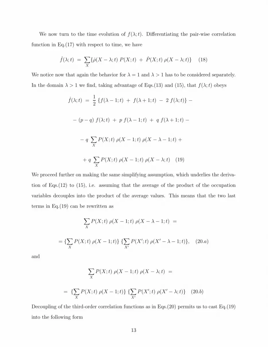
Equation (34) implicitly determines A as a function of p/q and ρ−. Numerical solution of

this equation is presented in Fig.3.

Now, a simple analysis shows that Eq.(34) has a unique positive solution for any p and

q which satisfy p > q(1 − ρ−), (or, since p = 1 − q, such q which are less than 1/(2 − ρ−)).

When p/q → 1 − ρ−, the parameter A → 0 as

A ≈√

2

π

p − q(1 − ρ−)

qρ−

, (35)

and is exactly equal to zero for p/q = 1−ρ−. It means that in the domain of parameters such

that p > q(1 − ρ−), the gas phase expands and the phase boundary moves as X(t) = A√

t,

A > 0. Before we turn to the analysis of the behavior of the PBP in the regime p < q(1−ρ−),

let us mention some other interesting aspects of Eqs.(34) and (32).

Time-dependent A (p/q = 1). We note that Eq.(34) predicts that A diverges loga-

rithmically when p/q → 1 (Fig.3). Nameley,

A ≈√

− 2 ln(1 − p

q), (36)

which means apparently that when p = q the parameter A is some increasing function

of time. This is, of course, consistent with the result of [29] which states that the mean

displacement of the PBP obeys X(t) ∼√

t ln(t) for the lattice gas with ρ− = 1 and p = q =

1/2. Let us now estimate, in terms of our approach, the behavior of A for arbitrary ρ− and

p = q = 1/2. For p = q our Eq.(16) reduces to

X(t) = f(ω = 0) (37)

Next, supposing that X(t) still follows the law X(t) = A√

t, in which the prefactor A may

be a slowly varying function of time, such that A/√

t → 0 when t → ∞, we find that the

representation of f(λ; t) in terms of a single scaled variable ω is still appropriate; weak time-

dependence of parameter A actually results in the appearence of vanishing in time correction

terms. We have then that the boundary condition in Eq.(25) reads

17

∂

∂ωf(ω)

∣

∣

∣

∣

∣

ω=0

≈ A3

2√

t, when t → ∞ (38)

On the other hand, we can calculate the derivative of f(ω) directly, using Eq.(32). This

gives

∂

∂ωf(ω)

∣

∣

∣

∣

∣

ω=0

≈ ρ−A√2π

exp(−A2/2) (39)

Comparing next the rhs of Eqs.(38) and (39), we infer that the parameter A obeys

A2 exp(A2/2) ≈√

2ρ2−t

π, (40)

which yields

A ≈√

ln(2ρ2

−t

π) (41)

Equation (41) thus generalizes the result of [29] for arbitrary initial mean density ρ−.

Wandering of the PBP in the critical case p/q = 1 − ρ−. Here we present some

heuristic estimates of the time evolution of the second moment of the distribution P (X; t)

in the case when the gas phase does not ”wet” the region X > 0, i.e. when X(t) = 0. To do

this, let us recall the Einstein relation between the diffusion coefficient D of a particle, which

performs an unconstrained symmetric random walk in absence of external forces, and the

mobility µ of the same particle in the case when an external constant force is present. The

Einstein relation states that µ = βD. Of course, it is not clear apriori whether the Einstein

relation between the diffusion coefficient and the mobility should hold also for the tracer

particle diffusing in a one-dimensional lattice gas; indeed, it may be invalidated because

of the hard-core interactions. This question has been addressed for the first time in [33],

in which work several important advancements have been made. To illustrate some of the

results obtained in [33], which are relevant to the model under study, let us first define the

mobility of the tracer particle:

µ = limt→∞µ(t), (42)

18

where µ(t) denotes

µ(t) = limF→0X(t)

Ft, (43)

i.e. µ(t) is the ratio of the mean displacement X(t) of the tracer particle, diffusing in the

presence of constant external force F , and F t; the ratio being taken in the limit when the

external force tends to the critical value (zero) at which the mean displacement vanishes.

Next, the diffusion coefficient of the tracer particle is defined by

D = limt→∞D(t) = limt→∞ {X2r (F = 0, t)

2t}, (44)

where X2r (F = 0, t) denotes the mean-square displacement of the tracer particle in the case

when the external force is equal to its critical value (zero). Now, for the tracer diffusion in

a one-dimensional hard-core lattice gas one has that X2r (F = 0, t) obeys Eq.(1), while X(t)

is determined by Eqs.(3) and (4).

One readily notices now that the Einstein relation holds trivially for infinitely large

systems, since here both µ and D are equal to zero [33]. A more striking result obtained in

[33] concerned the case when the one-dimensional lattice is a closed ring of length L. It was

shown that here both µ and D are finite, both vanish with the length of the ring as 1/L

and obey the Einstein relation µ(L) = βD(L) exactly! Next, [31] and subsequently, [32],

focused on the non-stationary behavior in infinite systems and showed that the Einstein

relation holds in an even more general sense: namely, the time-dependent mobility µ(t) and

the diffusivity D(t) obey

µ(t) = β D(t), (45)

at times t sufficiently large, such that the asymptotical regimes described by Eqs.(1) and

(3) are established.

Now, in the situation under study we have non-zero critical force (A = 0 when p =

q(1 − ρ−) or, in other words, when F = Fc = −β−1ln(1 − ρ−)). We thus define the time-

dependent mobility µ(t) as

19

µ(t) = limF→Fc

X(t)

(F − Fc) t, (46)

which yields, by virtue of Eq.(35), the following result

µ(t) = β1 − ρ−

ρ−

√

2

πt(47)

Assuming next that the generalized Einstein relation in Eq.(45) holds in the situation under

study, we find that in the critical case p = q(1 − ρ−) the mean-square displacement of the

PBP obeys:

X2r (F = Fc, t) =

1 − ρ−

ρ−

√

8t

π, (48)

which is surprisingly similar to the classic result in Eq.(1).

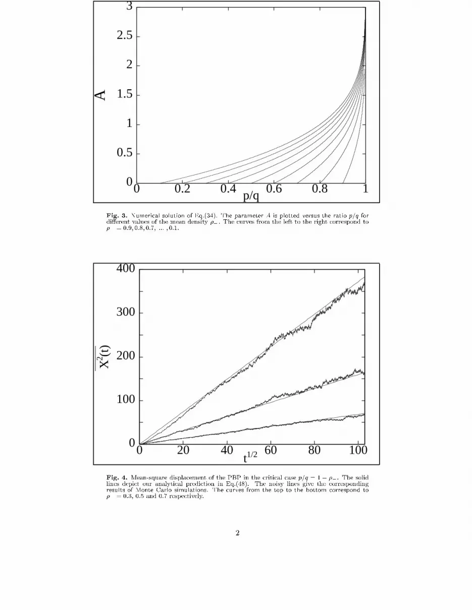
In Fig.4 we compare our analytical prediction in Eq.(48) against the results of Monte

Carlo simulations, performed at three different values of the gas phase densities ρ−. It

shows that our Eq.(48) is in a good agreement with the numerical results. This means that

the Einstein relation in Eq.(45) holds even in such a ”pathological” situation, in which the

critical value of the external force is not equal to zero and the particle density is different

from both sides of the test particle.

Density profiles. Let us now analyse the form of the density profiles as seen from the

PBP. In Figs.5 and 6 we plot the result in Eq.(32) versus the scaled variable ω for different

initial mean densities and different values of the ratio p/q.

In Fig.5 we depict f(ω) for fixed p/q = 0.9, which corresponds to fixed ”boundary

tension” force F , and different initial mean densities ρ−. In the range of used parameters,

all corresponding values of A are of the same order (A ≈ 1) and the density curves look

quite similar; starting from the same value at ω = 0, f(ω = 0) = 1 − p/q = 0.1, they

quite rapidly, within a few units of ω, approach their unperturbed initial values. We note,

however, that on the X-scale it does not mean that the density past the rightmost particle

rapidly reaches the unperturbed value ρ−. Instead, at sufficiently large times the density

stays almost constant and equal to 1 − p/q within a macroscopically large region ∼ X(t) .

20

Now, in Fig.6 we plot f(ω) versus ω in the opposite case when ρ− is fixed and the

”boundary tension” force is varied. Here the density profiles display rather strong depen-

dence on the parameter A. When A is small f(ω) shows almost linear dependence on ω

(curves (3) and (4)). The reason for such a behavior is that here the phase boundary moves

essentially slower (A < 1), compared to the typical displacements of the gas particles, which

then have sufficient time to equilibrate the density profile past the PBP. In the opposite case

of relatively large values of A, (A > 1), such an equilibration does not take place and the

dependence of f(ω) on ω is progressively more pronounced the larger A is.

It may also be worth-while to discuss the shapes of the density profiles in terms of the

variables λ and t. First, from Eq.(32) we have that in the limit of small ω, i.e. λ ≪ X(t),

the density obeys

f(λ; t) ≈ (1 − p

q) [1 +

A (λ − 1)√t

+ ... ], (49)

which means that past the PBP the density is almost constant in the region whose size

grows in proportion to X(t). Next, within the opposite limit, i.e. at distances λ which

exceed considerably X(t), we obtain from Eq.(32) the following result

f(λ, t) ≈ ρ− − (1 − p

q)

A√

2t

λexp(−λ2

2t) + ... (50)

Equation (50) shows that at large separations from the phase boundary the density ap-

proaches the unperturbed value ρ− exponentially fast. The approach is from below and is

weakly (only through the prefactors) dependent on the parameters p/q and A.

Mass of particles and mean density. We close this subsection with a brief analysis

of the time evolution of the integral characteristic of the propagating gas phase; namely, of

the ”mass” M(t) and the mean density ρmean = M(t)/X(t) of lattice gas particles at sites

X > 0 at time t.

The parameter M(t), which measures the amount of the gas-phase particles which

emerged up to time t in the previously empty half-line X > 0, is formally defined as

21

M(t) =∫ X(t)

0dX ρ(X; t) (51)

Changing the variable of integration, we find that M(t) can be rewritten as

M(t) =∫ X(t)

0dλ f(λ; t) =

= X(t)∫ 1

0dω f(ω) = M t1/2, (52)

where M is given by

M = A (1 − p

q) exp(A2/2) (53)

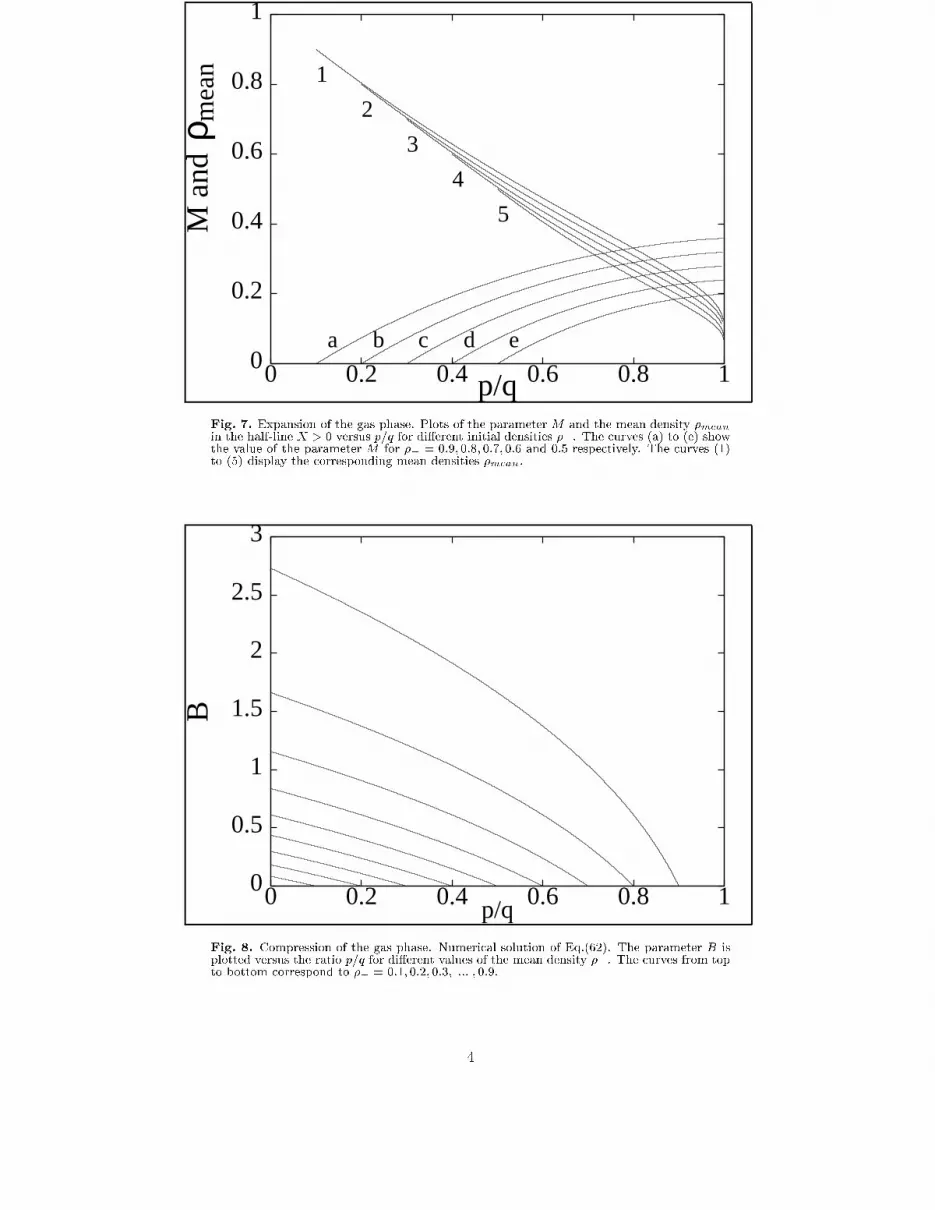
Figure 7 displays the plot of the prefactor M versus p/q and shows that M is a mono-

tonically increasing function of p/q. In contrast to the parameter A, M remains finite for

p = q, which means that bulk contribution to the ”mass”, as it could be expected intuitively,

comes from the lattice gas particles, whose motion is constrained by hard-core exclusions

and whose mean displacement grows only as√

t, without an additional logarithmic factor

which is specific only to the PBP.

Finally, we depict in Fig.7 the mean density on the interval X ∈ [0, X(t)] , defined as

ρmean =M(t)

X(t)= (1 − p

q) exp(A2/2) (54)

Figure 7 shows that despite of the exponential factor exp(A2/2) the mean density ρmean

rapidly decreases with an increase of p/q and is a slowly increasing function of ρ−.

B. Compression of the gas phase.

Let us next address the question of the PBP dynamics in the case p < q(1 − ρ−), when

X(t) is expected to be less than zero and thus the gas phase to be effectively compressed

by the ”boundary tension” force exerted on the PBP. Recollecting the results of [30–32]

we suppose that here X(t) obeys X(t) = −B√

t, B > 0, and define the scaled variable as

22

ω = (λ−1)/B√

t, where ω is positive definite 0 ≤ ω ≤ ∞. In terms of this variable Eqs.(24)

takes the form

∂2

∂ω2f(ω) + B2 (ω + 1)

∂

∂ωf(ω) = 0, (55)

while the boundary condition in Eq.(25) reads

∂

∂ωf(ω)

∣

∣

∣

∣

∣

ω=0

= −B2 f(ω = 0) (56)

Again, the boundary and initial conditions in Eqs.(23.b) and (23.c) collapse into a single

Eq.(28).

The general solution of Eq.(55) can be written down as

f(ω) = C1

∫ ω

0dz exp(−B2

2(z2 + 2z)) + C2, (57)

where C1 and C2 are to be chosen in such a way that Eqs.(28) and (56) are satisfied. Inserting

Eq.(55) into Eqs.(28) and (56) we then obtain

C1 = − B2 C2, (58)

and

C2 = ρ− {1 − B2∫ ∞

0dz exp(−B2

2(z2 + 2z))}−1 (59)

Consequently, the density profile past the PBP can be expressed in terms of B and ω as

f(ω) = ρ− {1 − B2∫ ω

0dz exp(−B2

2(z2 + 2z))}/

/{1 − B2∫ ∞

0dz exp(−B2

2(z2 + 2z))} (60)

Next, Eq.(16) implies that also in this case f(ω = 0) → (q − p)/q as t → ∞, which yields

eventually the following closed-form equation for the parameter B:

1 − B2∫ ∞

0dz exp(−B2

2(z2 + 2z)) =

qρ−

q − p(61)

23

Equation (61) can be put into a more compact form if we express the integral over dz in

terms of the probability integral. We then obtain

I−(B) =q(1 − ρ−) − p

q − p, (62)

where I−(B) is defined in Eq.(10). In Fig.8 we present the numerical solution of Eq.(62),

plotting the prefactor B as a function of the ratio p/q at different values of the density ρ−.

Equation (62) resembles the form of Eq.(34), which determines the parameter A, but

differs from it in two aspects; first, the rhs of Eq.(62) is exactly the rhs of Eq.(34) but taken

with the opposite sign, which insures that B is positive for p < q(1 − ρ−), and second, the

sign before the probability integral in brackets is opposite to that in Eq.(34). The latter

circumstance is responsible for the fact that B tends to the limiting value Blim when q → 1

(p → 0). When q → p/(1 − ρ−) the parameter B tends to zero exactly in the same way as

the parameter A in Eq.(35) taken with the opposite sign, which means that the prefactor

in X(t) does not have a discontinuity at the ”critical” point p/q = 1− ρ− both for its value

and for its slope.

Now, in the limit q = 1 (p = 0), Eq.(62) reduces to

√

π

2Blim exp(B2

lim/2) [1 − Φ(Blim/√

2)] = 1 − ρ−, (63)

which was obtained previously in [30,31] (see Eq.(2) in the present paper). Within the limit

ρ− → 1 Eq.(63) yields

Blim ≈√

2

π(1 − ρ−), (64)

which shows that Blim, as it could be expected intuitively, tends to zero when the density

tends to 1.

When the gas is very dilute, i.e. ρ− ≪ 1, we may expect that Blim is large. Expanding

the probability integral as

Φ(Blim/√

2) ≈ 1 −√

2

πB−1

lim exp(−B2lim/2) +

24

+

√

2

πB−3

lim exp(−B2lim/2) − ... , (65)

we find, upon substitution of Eq.(65) into the Eq.(63), the following result

Blim ≈ 1√

ρ−

, (66)

i.e. Blim diverges when ρ− → 0 in proportion to the inverse of the square-root of the particle

mean density. In Fig.9 we present the numerical solution of Eq.(63) together with the results

of Monte Carlo simulations. Obviously, the agreement is very good.

Finally, in Fig.10 we combine the results of the subsections A and B and plot both analyt-

ical and Monte Carlo results obtained for the dependence of the prefactor α(F ) = X(t)/√

t

on the ratio p/q and the density ρ−. Again, we find very good agreement between our ana-

lytical predictions and numerical results, which support the validity of the approximations

involved in our analysis.

Density profiles. Consider now the density profiles as seen from the PBP in the

compression regime. In Fig.11 we plot f(ω) versus ω for different values of p/q at fixed ρ−.

Figure 11 shows that similarly to the behavior in the expansion regime, the density

profiles are quite sensitive to the value of the parameter B. When B is smaller than unity,

f(ω) shows almost linear dependence on ω, while in the case when B > 1 this dependence

is non-linear and f(ω) rapidly drops from f(ω = 0) = 1 − p/q to ρ−.

We finally present explicit results for f(λ; t). In the limit of small λ, such that λ ≪

X(t)/B2, we have

f(λ; t) ≈ (1 − p

q) [1 − B(λ − 1)√

t+ ... ], (67)

which shows that the density is almost constant, (being only slightly less than (1 − p/q)),

in the spatial region whose size is of the order of the PBP mean displacement.

For large λ we obtain from Eq.(60)

f(λ; t) ≈ ρ− + (1 − p

q)

B√

2t

λexp(−λ2/2t) + ... , (68)

25

i.e. similarly to the behavior in the expansion regime, the density approaches the un-

perturbed value ρ− exponentially fast and with a rate which is weakly (only through the

pre-exponential factor) dependent on the parameter B and the ratio p/q.

V. DYNAMICAL EQUATIONS IN THE PRESENCE OF THE LOW-DENSITY

PHASE.

Let us now consider the time evolution of the local density ρ(X; t) and of the probability

distribution P (X; t) in the general case when the LDP is present and ρ− ≥ ρ+ ≥ 0.

One readily notices that also in this case Eq.(12) and, consequently, Eq.(13), describe

the time evolution of the realization-averaged occupation variable ρ(X; t) for all X excluding

the sites X = X(t)±1. Dynamical equation describing evolution of ρ(X; t) at X = X(t)−1

will be, however, somewhat modified as compared to Eq.(14). We have here

ρ(X(t) − 1; t) =1

2(ρ(X(t) − 2; t) − ρ(X(t) − 1; t)) +

+ q (1 − ρ(X(t) − 1; t)) ρ(X(t) − 2; t) −

− p (1 − ρ(X(t) + 1; t)) ρ(X(t) − 1; t), (69)

in which we account that the hops of the PBP in positive direction can be constrained by

the LDP particles by introducing a factor (1 − ρ(X(t)+ 1; t)). In a similar fashion, we find

that at the site X = X(t) + 1 the local particle density obeys

ρ(X(t) + 1; t) =1

2(ρ(X(t) + 2; t) − ρ(X(t) + 1; t)) −

− q (1 − ρ(X(t) − 1; t)) ρ(X(t) + 1; t) +

+ p (1 − ρ(X(t) + 1; t)) ρ(X(t) + 2; t) (70)

Next, for the time evolution of the distribution function P (X; t) we obtain the following

equation

26

P (X; t) = − P (X; t) [p (1 − ρ(X + 1; t)) + q (1 − ρ(X − 1; t))] +

+ (1 − ρ(X; t)) [p P (X − 1; t) + q P (X + 1; t)], (71)

which differs from the corresponding equation of the previous sections, Eq.(15), by the

factors (1 − ρ(X + 1; t)) and (1 − ρ(X; t)) in the first and third terms respectively; these

factors account, in a mean-field-type fashion, for the fact that hops of the PBP in the positive

direction can take place only if the corresponding lattice sites are free of the LDP particles

at this moment of time.

Further on, multiplying both sides of Eq.(71) by X and summing over all lattice sites we

have that the mean displacement of the PBP obeys:

X(t) = p − q − p f(λ = −1; t) + q f(λ = 1; t), (72)

which thus generalizes Eq.(16) for the case of non-zero density of the LDP; the factor f(−1; t)

on the right-hand-side of Eq.(72) accounts for the hindering effects of the LDP particles on

the PBP dynamics.

Consider now the time evolution of the correlation function f(λ; t), defined in Eq.(17).

By virtue of Eqs.(18), (13) and (71) we find that the evolution of this property is guided by:

f(λ; t) =1

2[f(λ + 1; t) + f(λ − 1; t) − 2 f(λ; t)] −

− f(λ; t) [1 − p f(−1; t) − q f(1; t)] +

+ p f(λ − 1; t) [1 − f(−1; t)] + q f(λ + 1; t) [1 − f(1; t)], (73)

which holds for all λ excluding λ = ±1. In the limit ρ− → 0, i.e when f(−1; t) → 0, this

equation reduces to Eq.(21). In the continuous-space limit Eq.(73) attains the form

f(λ; t) =1

2

∂2f(λ; t)

∂λ2− [p − q − p f(−1; t) + q f(1; t)]

∂f(λ; t)

∂λ(74)

which is exactly Eq.(24) with X(t) defined by Eq.(72).

27

Further on, we find that the correlation function f(λ; t) at the left-hand adjacent to the

PBP site (for λ = 1) obeys

f(1; t) =1

2(f(2; t) − f(1; t)) + p f(0; t) (1 − f(−1; t)) −

− q f(1; t) (1 − f(1; t)) − 2 p f(1; t) (1 − f(−1; t)) +

+ 2 q f(2; t) (1 − f(1; t)) (75)

Comparing now Eq.(75) with Eq.(73) we have the following condition on f(λ; t) at λ = 1:

1

2(f(0; t) − f(1; t)) = q f(2; t) (1 − f(1; t)) − p f(1; t) (1 − f(−1; t)) (76)

Next, from Eqs.(18), (70) and (71) we can derive

f(−1; t) =1

2(f(−2; t) − f(−1; t)) −

− p f(−1; t) (1 − f(−1; t)) − 2 q f(−1; t) (1 − f(1; t)) +

+ 2 p f(−2; t) (1 − f(−1; t)) + q f(0; t) (1 − f(1; t)), (77)

which allows us to deduce the boundary condition on f(λ; t) at the point λ = −1:

1

2(f(0; t) − f(−1; t)) = − q f(−1; t) (1 − f(1; t)) +

+ p f(−2; t) (1 − f(−1; t)) (78)

In the continuous-space limit Eqs.(76) and (78) reduce to

1

2

∂f(λ; t)

∂λ

∣

∣

∣

∣

∣

λ=±1

= X(t) f(±1; t), (79)

which represent two boundary conditions for the continuous-space Eq.(74). Equations (74)

and (79), with the initial conditions

28

f(λ; t)|t=0 = ρ+ for λ < 0, (80.a)

f(λ; t)|t=0 = ρ− for λ > 0, (80.b)

and the boundary conditions

f(λ; t)|λ→∞ = ρ−, (81.a)

f(λ; t)|λ→−∞ = ρ+, (81.b)

constitute a closed system of equations which allows to compute X(t) and the density profiles

for arbitrary relation between p and q, as well as for arbitrary ρ+ and ρ−.

VI. SOLUTION OF DYNAMICAL EQUATIONS IN THE GENERAL CASE

ρ− ≥ ρ+ ≥ 0.

In this section we will derive explicit results for the dynamics of the mean displacement

of the PBP and also for the density distribution around it. As it was done in the previous

sections, we will discuss separately the behavior in the case when the HDP expands, com-

pressing the LDP, and when, on the contrary, the LDP and the external force F compress

the HDP.

A. Expansion of the high-density phase.

We again set X(t) = A√

t and suppose first that A ≥ 0. Conditions at which such a

behavior takes place will be specified below. For λ ≥ 1 (past the PBP) we then have

f(ω) =ρ−

1 + I+(A){1 + A2

∫ ω

0dz exp(−A2

2(z2 − 2z)}, (82)

where ω = (λ−1)/A√

t and I+(A) is defined in Eq.(10). In front of the PBP, i.e. for λ ≤ −1,

the scaled density profile is given by

29

f(θ) =ρ+

1 − I−(A){1 − A2

∫ θ

0dz exp(−A2

2(z2 + 2z)}, (83)

in which we have denoted θ = −(λ + 1)/A√

t and I−(A) is made explicit in Eq.(10). The

density distributions f(ω) and f(θ) for different values of the parameters A, ρ± and p (q)

are depicted in Figs.5,6 and 11 respectively.

Equations (82) and (83) contain the parameter A, which has not yet been specified. To

determine A we take advantage of Eq.(72) which yields the following condition on the local

densities at the sites adjacent to the PBP position:

q (1 − f(λ = 1; t)) = p (1 − f(λ = −1; t)) (84)

Upon substitution of Eqs.(82) and (83) into the latter equation we find that A (in case when

A ≥ 0) obeys the following transcendental equation:

q ρ−

1 + I+(A)− p ρ+

1 − I−(A)= q − p, (85)

which generalizes our Eq.(34) and also the result of [31] (Eq.(4) of the present paper) for

the case when the particle densities from the left and from the right of the PBP are different

and the density of the LDP is not zero. One directly verifies that Eq.(85) reduces to Eq.(34)

when we set ρ+ = 0, while setting ρ+ = ρ− we recover Eq.(4).

Let us now find the conditions under which the parameter A is positive, i.e. the HDP

expands. To do this, we simply notice that when A = 0 both I+(A) and I−(A) are equal to

zero, which means that the ”critical” relation between p, q and ρ± is:

q (1 − ρ−) = p (1 − ρ+) (86)

Equation (86) implies that A vanishes, (i.e. the LDP and the HDP are in equilibrium with

each other), when the probability of the PBP to go towards the HDP times the density of

vacancies in this phase is exactly equal to the probability of going towards the LDP times

the density of vacancies in this phase. When p(1 − ρ+) ≥ q(1 − ρ−) the HDP expands.

We note that Eq.(86) was previously obtained in [33] from the analysis of the stationary

states in a one-dimensional lattice gas placed in a finite box of length L. By explicit calcula-

tion of the distribution function of the PBP position in the general case when the numbers

30

of the lattice gas particles from the right and from the left of the PBP are not equal, it was

found [33] that in the limit L → ∞ the PBP is localized at point X0, which divides the

system in proportion given by Eq.(86).

Equation (86) can also be rewritten using the definition of the external force F . Upon

some algebra, we find then that the critical force at which both phases are in equilibrium

with each other is given by

Fc = β−1 ln(1 − ρ+

1 − ρ−

) (87)

Now, let us discuss the behavior of the parameter A in the limit when A is small or large,

and calculate the diffusivity of the PBP in the critical case A = 0. In the limit of small A,

i.e. when p, q and ρ± are close to their ”critical” values determined by Eqs.(86) and (87),

both I±(A) ≈√

π/2A. Substituting these expressions into Eq.(85) we find

A ≈√

2

π

p(1 − ρ+) − q(1 − ρ−)

qρ− + pρ+

, (88)

which is valid when A ≪ 1. Eq.(88) allows for the computation of the PBP mobility, which

we determine following the arguments presented in Section IV as

µ(t) = limF→Fc

X(t)

(F − Fc) t=

= t−1/2 limF→Fc

A

(F − Fc)(89)

Substituting Eq.(88) into Eq.(89) and taking the limit F → Fc, we find

µ(t) = β(1 − ρ−)(1 − ρ+)

(ρ− + ρ+ − 2ρ−ρ+)

√

2

πt, (90)

which yields, by virtue of Eq.(45), the result presented in Eq.(7). Eq.(7) generalizes the

classical result in Eq.(1) for the situation in which the mean particles densities for both

sides of the tracer particle are different from each other. One can directly verify that Eq.(7)

reduces to Eq.(1) when ρ− = ρ+, while setting ρ+ = 0 we recover our previous result

in Eq.(48). In Fig.12 we compare our analytical prediction in Eq.(90) against the results

31

of Monte Carlo simulations, which shows that an approximate approach developed here

represents a fair description of the PBP dynamics.

Next, in Section IV we have demonstrated that the prefactor A diverges when p → q.

Consequently, we can expect that even in the presence of the LDP the prefactor A can attain

large values when ρ+ ≪ 1 and p/q → 1. Setting in Eq.(85) q = p and using the expansion

in Eq.(65) we find from Eq.(85) that A is defined in the limit ρ+ → 0 by

A ≈√

2 ln(ρ−/ρ+), (91)

i.e. A grows as a square-root of the logarithm of ρ+ when ρ+ → 0.

Finally, we estimate the behavior of the ratio δ of the particle densities immediately past

and in front of the PBP. At zero moment of time this ratio is evidently δ = δ0 = ρ−/ρ+.

Our results in Eqs.(82) and (83) suggest that after some transient period of time the density

profiles past and in front of the PBP attain stationary forms with respect to the variable

ω = (λ− 1)/X(t). Consequently, we have that, as the time evolves, the ratio of the particle

densities immediately past and in front of the PBP tends to a constant value

δ = δ01 − I−(A)

1 + I+(A)(92)

Eq.(92) holds for arbitrary values of A. In the asymptotic limits when A is small or large,

we find from Eq.(92) the following explicit asymptotic forms for δ:

δ ≈ δ0 (1 − (π

2− 1) A2 + ... ), when A ≪ 1, (93)

and

δ ≈ δ0exp(−A2/2)√

2πA3when A ≫ 1 (94)

Therefore, the parameter δ, as it could be expected intuitively, is always less than δ0. Com-

plete dependence of δ on the parameter A is presented in Fig.14.

32

B. Compression of the high-density phase.

Consider now the behavior in the regime when the LDP and the applied force compress

the HDP. Setting X(t) = −B√

t, where B is supposed to be a positive constant, we find

from Eqs.(74) and (79) that the particle density for λ ≥ 0 (i.e. at sites X < X(t)) obeys

Eq.(60), in which the variable ω is defined as ω = (λ − 1)/B√

t and the parameter A is

replaced by B. From the other side of the PBP, i.e for λ ≤ 0, we have

f(θ) =ρ+

1 + I+(B){1 + B2

∫ θ

0dz exp(−B2

2(z2 − 2z))}, (95)

where the scaled variable θ = −(λ + 1)/B√

t. The function f(θ) is depicted in Figs.5 and

6. Substituting Eqs.(60) and (95) into Eq.(84) we arrive at the following transcendental

equation for the parameter B:

q ρ−

1 − I−(B)− p ρ+

1 + I+(B)= q − p (96)

Eq.(96) thus generalizes the result in Eq.(62) for the case of the non-zero particles density

in the LDP.

Now, noticing that Eqs.(96) and (85) can be cast into one another by the substitution

±I±(A) → ∓I∓(B), we can construct a general equation for the parameter α(F ) in Eq.(3).

This equation is presented in Eq.(6) and holds for arbitrary relation between ρ± and p/q,

describing hence both the expansion and the compression regimes. In Fig.13 we present the

numerical solution of Eq.(6), plotting α(F ) as a function of the ratio p/q for different values

of ρ− and ρ+.

Finally, we analyze the behavior of the parameter δ, which is defined as the ratio of the

particle density immediately past the PBP and the particle density immediately in front of

the PBP. Using Eqs.(60) and (95) we find

δ = δ01 + I+(B)

1 − I−(B)(97)

Numerical plot of δ(B) is presented in Fig.14.

33

Asymptotic behavior of the parameter δ in the limits when B is small or large readily

follows from our Eqs.(93) and (94). Here we have

δ ≈ δ0 (1 + (π

2− 1) B2 + ... ), when B ≪ 1, (98)

and

δ ≈ δ0

√2π B3 exp(B2/2), when B ≫ 1, (99)

which means that in the compression regime the parameter δ is always greater than δ0.

VII. MONTE CARLO SIMULATIONS.

In order to check our analytical predictions, derived in terms of a mean-field approxima-

tion, we have performed Monte Carlo simulations of the process defined in the begining of

Section II. The simulation algorithm was defined as follows:

We constructed first a one-dimensional regular lattice of unit spacing and length 2L+1,

sites of which were labelled by integers of the interval [−L, L]. In all simulations we took

L = 103. At the zero moment of the MC time the particles were placed randomly on the

lattice with the prescribed mean densities and the constraint that two particles can never

simultaneously occupy the same site. To do this, we have called, for each lattice site from

the interval [−L + 1,−1] independently, a random number from the interval [0, 1]. In case

when the random number produced by the generator was less that ρ− a particle was created

on this lattice site. In case when the random number was greater than ρ− the site was left

empty. The same routine was performed for the sites with positive numbers [1, L− 1]; here

a particle was created at the corresponding site in case when the random number was less

than ρ+ and the site was left empty if the random number was greater than ρ+. The phase

boundary particle was placed at the origin. Additionally, we have prescribed that the sites

X = ±L are occupied by particles. The particles at theses sites X = ±L are made immobile,

blocking the lattice from both sides and preventing other particle to leave the system.

34

The subsequent particle dynamics employed in our simulations follows the definitions of

Section 2 closely. We call for a random integer number X from the interval [−L + 1, L− 1].

Here three different events may take place:

(i) If the site X is vacant, a new site is considered.

(ii) If the site X is occupied by a particle, we first increase the MC time by unity and

then let the particle choose, at random, a potential jump direction. This is done again by

calling a random number from the interval [0, 1]. If the random number is less than 0.5,

the particle attempts to jump to the site X − 1; otherwise, it attempts to jump to the site

X +1. The jump is fulfilled if at this moment of the MC time the adjacent site in the chosen

direction is vacant (not occupied by any other particle or the PBP). Otherwise, the particle

remains at X.

(iii) If the site X appears to be occupied by the PBP, we increase the MC time by unity

and consider a random number from the interval [0, 1]; in case when this number is less than

the prescribed value q, the PBP attempts to jump to the site X − 1. Otherwise, it attempts

to jump to the site X + 1. The jump is fulfilled if at this moment of MC time the adjacent

site in the chosen direction is vacant. Otherwise, the PBP remains at X.

In simulations we have followed the time evolution of several different properties: the

PBP displacement, squared displacement (under the critical conditions) and the occupations

of the sites X = ±L ∓ 100. Time behavior of these properties was plotted versus the

”physical time” t, which is the time needed for each particle to move once, on average, or

in other words, t = MCtime/number of particles. We have observed that for all values of

the parameters ρ± and q, used in our simulations, the stationary regime in which the ratio

Xr(t)/√

t approaches a constant value is established for displacements of order of 200 lattice

units. To get the spatially resolved behavior, in computation of the PBP displacement

each realization of the process was interrupted at the moment when the absolute value

of the PBP displacement reaches the value of 500 lattice. For calculation of the mean

displacement we used typically 102 realizations for each set of parameters ρ± and q. Results

of these simulations are presented in Figs.9 and 10. Further on, computing the squared

35

displacement we interrupted each realization of the process at the moment when the span

of the PBP trajectory is equal to 102. Mean-square displacement was obtained by averaging

over 2 × 103 realizations. Results for mean-square displacement of the PBP are presented

in Figs.4 and 12. In all cases, we have obtained remarkably good agreement between our

analytical predictions and simulation results. Finally, the measurements of the occupations

of the sites X = ±L∓100 were performed in order to be sure that the perturbances created

by the PBP do not spread during the simulation time through the whole system and do

not lead to artificial behaviors associated with the finite-size effects. We have observed

that actually the mean densities of these sites don’t vary with time and are equal to the

unperturbed values ρ±.

VIII. CONCLUSIONS.

To conclude, we have examined in terms of a mean-field-type approach the dynamics

of the phase boundary propagation in a one-dimensional hard-core lattice gas which was

initially put into a non-equlibrium, ”shock”-like configuration and then allowed to evolve

in time by particles attempting to hop to neighboring unoccupied sites. The ”shock” con-

figuration means that particle mean densities from the left and from the right of the origin

are different. All particles of the lattice gas, except the particle separating the high- and

the low-density phases, have symmetric hopping probabilities, while the phase boundary

particle is subject to a constant force F and has asymmetric hopping probabilities. We have

shown that the mean displacement of the PBP follows the generic law X(t) = α(F )√

t, in

which the parameter α(F ) can be both positive and negative, depending on the relation

between the magnitude of the force and the initial mean densities. This prefactor is deter-

mined implicitly, in a form of the transcendental Eq.(6) for arbitrary magnitude of the force

and arbitrary relation between the particle densities in the high- and low-density phases. In

several asymptotic limits we find explicit formulae for the prefactor. Further on, we have

shown that when F is equal to the critical value Fc, Eq.(87), the parameter α(F ) is exactly

36

equal to zero. In this case the high- and the low-density phases are in equilibrium with each

other. We have found that here the mean-square displacement X2r (t) of the PBP follows

X2r (t) ∼ γ

√t, i.e. shows a sub-diffusive behavior. The form of the prefactor γ is determined

explicitly, Eq.(7). Our analytical findings are in a very good agreement with the results of

numerical simulations.

The authors wish to thank J.L.Lebowitz and R.Kotecky for helpful and encouraging dis-

cussions. Financial support from the FNRS and the COST Project D5/0003/95 is gratefully

acknowledged.

[1] M.C.Cross and P.C.Hohenberg, Rev. Mod. Phys. 65, 851 (1993)

[2] M.Ben-Amar, P.Pelce and P.Tabeling, Nonlinear Phenomena Related to Growth and Form

(Plenum, New York, 1991)

[3] Y.Pomeau and M.Ben Amar, in Solids Far from Equilibrium, ed.: C.Godreche (Cambridge

University Press, Cambridge, 1992)

[4] A.M.Cazabat, F.Heslot, S.M.Troian and P.Carles, Nature 346, 824 (1990)

[5] J.S.Langer, in Chance and Matter, eds.: J.Souletie, J.Vannimenus and R.Stora (North-Holland,

Amsterdam, 1987)

[6] P.Collet and J.P.Eckmann, Instabilities and Fronts in Extended Systems (Princeton University

Press, Princeton, 1990)

[7] P.Collet, in: Wetting Phenomena, eds.: J.De Coninck and F.Dunlop (Springer-Verlag, Berlin,

1990)

[8] P.Devillard and H.Spohn, Europhys. Lett. 17, 113 (1992)

[9] M.Kardar and J.O.Indekeu, Europhys. Lett. 12, 161 (1990)

37

[10] A.Malevanets, A.Careta and R.Kapral, Phys. Rev. E 52, 4724 (1995)

[11] J.Armero, J.M.Sancho, J.Casademunt, A.M.Lacasta, L.Ramirez-Piscina and F.Sagues, Phys.

Rev. Lett. 76, 3045 (1996)

[12] U.Ebert, W.van Saarloos and C.Caroli, Phys. Rev. Lett. 77, 4178 (1996)

[13] J.L.Lebowitz, E.Presutti and H.Spohn, J. Stat. Phys. 51, 841 (1988)

[14] F.J.Alexander, C.A.Laberge, J.L.Lebowitz and R.K.P.Zia, J. Stat. Phys. 82, 1133 (1996)

[15] J.Hardy, O.de Pazzis and Y.Pomeau, Phys. Rev. A 13, 1949 (1976)

[16] U.Frisch, B.Hasslacher and Y.Pomeau, Phys. Rev. Lett. 56, 1505 (1986)

[17] C.Appert and S.Zaleski, Phys. Rev. Lett. 64, 1 (1990)

[18] D.H.Rothman and J.M.Keller, J. Stat. Phys. 52, 1119 (1988)

[19] G.Giacomin and J.L.Lebowitz, Phys. Rev. Lett. 76, 1094 (1996)

[20] G.Giacomin and J.L.Lebowitz, J. Stat. Phys. 87, 37 (1997)

[21] M.Z.Guo, G.C.Papanicolaou and S.R.S.Varadhan, Commun. Math. Phys. 118, 31 (1988)

[22] S.F.Burlatsky, G.Oshanin, A.M.Cazabat and M.Moreau, Phys. Rev. Lett. 76, 86 (1996)

[23] S.F.Burlatsky, G.Oshanin, A.M.Cazabat, M.Moreau and W.P.Reinhardt, Phys. Rev. E 54,

3832 (1996)

[24] T.E.Harris, J. Appl. Prob. 2, 323 (1965)

[25] D.B.Abraham, P.Collet, J.De Coninck and F.Dunlop, Phys. Rev. Lett. 65, 195 (1990)

[26] D.B.Abraham, P.Collet, J.De Coninck and F.Dunlop, J. Stat. Phys. 61, 509 (1990)

[27] J.De Coninck and F.Dunlop, J. Stat. Phys. 47, 827 (1987)

[28] G.Oshanin, J.De Coninck, A.M.Cazabat and M.Moreau, Phys. Rev. E 58, R20 (1998); J. of

38

Mol. Liquids 76, 195 (1998)

[29] R.Arratia, Z. Ann. Probab. 11, 362 (1983)

[30] S.F.Burlatsky, G.Oshanin, A.Mogutov amd M.Moreau, Phys. Lett. A 166, 230 (1992)

[31] S.F.Burlatsky, G.Oshanin, M.Moreau and W.P.Reinhardt, Phys. Rev. E 54, 3165 (1996)

[32] C.Landim, S.Olla and S.B.Volchan, Commun. Math. Phys. 192, 287 (1998)

[33] P.Ferrari, S.Goldstein and J.L.Lebowitz, Diffusion, Mobility and the Einstein Relation, in:

Statistical Physics and Dynamical Systems, eds.: J.Fritz, A.Jaffe and D.Szasz (Birkhauser,

Boston, 1985) p.405

[34] H.Spohn, Large Scale Dynamics of Interacting Particles, (Springer Verlag, New York, 1991),

Ch.3

39

0

p q1/2 1/2

"phase boundary" particle

ρ1/2

ρ+1/2

X

-

Fig. 1. Initial "sho k" on�guration of the latti e gas parti les: �� is the mean density ofparti les at the half-line �1 < X < 0 and �+, (�+ � ��), is the mean density of parti lesat the half-line 0 < X <1. All gas parti les, ex luding the "phase boundary" parti le, haveequal (= 1=2) probabilities for jumps to the right and to the left. The PBP has asymmetri hopping probabilities.

X0

"phase boundary" particle

p q1/2 1/2

Fig. 2. Initial "sho k" on�guration of the latti e gas parti les. All parti les are pla ed atrandom positions and at a �xed mean density �� from the left to the origin of the latti e,i.e. at sites X < 0. All sites X > 0 are va ant at t = 0.1

0

0.5

1

1.5

2

2.5

3

0 0.2 0.4 0.6 0.8 1

A

p/qFig. 3. Numeri al solution of Eq.(34). The parameter A is plotted versus the ratio p=q fordi�erent values of the mean density ��. The urves from the left to the right orrespond to�� = 0:9; 0:8; 0:7; ::: ; 0:1.

0

100

200

300

400

0 20 40 60 80 100

X (

t)2

____

__

t1/2Fig. 4. Mean-square displa ement of the PBP in the riti al ase p=q = 1 � ��. The solidlines depi t our analyti al predi tion in Eq.(48). The noisy lines give the orrespondingresults of Monte Carlo simulations. The urves from the top to the bottom orrespond to�� = 0:3, 0:5 and 0:7 respe tively. 2

0

0.2

0.4

0.6

0.8

1

0 0.5 1 1.5 2 2.5 3

f(

)ω

- - -

-

ω

ρ = 0.9ρ = 0.8ρ = 0.7

ρ = 0.5

p/q = 0.9

Fig. 5. Expansion of the gas phase. Plot of f(!), Eq.(32), versus ! = (� � 1)=X(t) at a�xed ratio p=q and variable ��. The orresponding values of the parameter A for the urvesfrom the top (�� = 0:9) to the bottom (�� = 0:5) are A = 1:37; 1:3; 1:25 and 1.

0

0.2

0.4

0.6

0.8

1

0 1 2 3 4 5 6

f(

)ω

ω

ρ = 0.9 -

(4)

(3)

(2)

(1)(1) p/q = 0.8(2) p/q = 0.6(3) p/q = 0.4(4) p/q = 0.2

Fig. 6. Expansion of the gas phase. Plot of f(!), Eq.(32), versus ! at �xed density �� = 0:9and variable ratio p=q. The orresponding values of the parameter A are 0:09 (4), 0:31 (3),0:58 (2) and 1 (1). 3

0

0.2

0.4

0.6

0.8

1

0 0.2 0.4 0.6 0.8 1

M a

nd

mea

nρ

p/q

a b c d e

1

2

3

4

5

Fig. 7. Expansion of the gas phase. Plots of the parameter M and the mean density �meanin the half-line X > 0 versus p=q for di�erent initial densities ��. The urves (a) to (e) showthe value of the parameter M for �� = 0:9; 0:8; 0:7; 0:6 and 0:5 respe tively. The urves (1)to (5) display the orresponding mean densities �mean.

0

0.5

1

1.5

2

2.5

3

0 0.2 0.4 0.6 0.8 1

B

p/qFig. 8. Compression of the gas phase. Numeri al solution of Eq.(62). The parameter B isplotted versus the ratio p=q for di�erent values of the mean density ��. The urves from topto bottom orrespond to �� = 0:1; 0:2; 0:3; ::: ; 0:9.4

0

1

2

3

4

5

0 0.2 0.4 0.6 0.8 1

Blim

ρFig. 9. Plot of the parameter B lim versus the mean parti le density ��. The solid lineshows the numeri al solution of Eq.(63). The diamonds represent the asso iated MonteCarlo simulation results.

-1

-0.5

0

0.5

1

1.5

0 0.2 0.4 0.6 0.8 1

X(t

)/t1/

2

p/qFig. 10. Theoreti al and experimental results for the prefa tor in the dependen e X(t) =�(F )pt as the fun tion of the ratio p=q. The urves from top to bottom orrespond todi�erent values of the density ��: the upper urve gives �(F ) for �� = 0:6, the lower urve orresponds to �� = 0:4 and the urve in the middle - to �� = 0:5. Symbols denote theresults of Monte Carlo simulations. 1

0

0.2

0.4

0.6

0.8

1

0 0.5 1 1.5 2 2.5 3

f(

)ω

ω

(1)

(2)

(3)

(4)

ρ = 0.2 - (1) p/q = 0.1(2) p/q = 0.3(3) p/q = 0.5(4) p/q = 0.7

Fig. 11. Compression of the gas phase. Plot of f(!), Eq.(60), versus the s aled variable ! at�xed density �� = 0:2 and variable ratio p=q. The orresponding values of the parameter Bare 1:52 (1), 1:21 (2), 0:83 (3) and 0:34 (4).

0

40

80

120

0 20 40 60 80 100

X (

t)2

____

__

t1/2Fig. 12. Mean-square displa ement of the PBP in the riti al ase p=q = (1� ��)=(1 � �+),Eq.(86). The solid lines show our analyti al predi tion from Eq.(7) and the noisy lines givethe results of Monte Carlo simulations. The urves from top to bottom orrespond to thefollowing values of the parameters (��; �+): The �rst two urves are the analyti al result inEq.(1) and numeri al data for the symmetri ases (0:4; 0:4) and (0:5; 0:5). The lower urves orrespond to (0:6; 0:5), (0:9; 0:4),(0:7; 0:5) and (0:8; 0:2) respe tively.2

-0.8

-0.4

0

0.4

0.8

0 0.4 0.8 1.2 1.6 2

X(t

)/t1/

2

p/q

(1)

(2)

(3)(4)

Fig. 13. Numeri al solution of Eq.(6). Prefa tor �(F ), Eq.(3), is plotted versus the ratiop=q for di�erent initial mean densities from the left and from the right of the origin. The urves from (1) to (4) orrespond respe tively to (�� = 0:9; �+ = 0:3), (0:8; 0:2), (0:7; 0:3)and (0:5; 0:5).

0

2

4

6

8

10

0 0.2 0.4 0.6 0.8 1

0δ

/ δ

A, B

(1)

(2)Fig. 14. Plot of the parameter Æ, Eqs.(92) and (97), versus the parameters A and B. The urve (1) des ribes the behavior of Æ(B) in the ompression regime. The urve (2) de�nesÆ(A) in the expansion regime. 3