Journal of Applied Geophysics 93 (2013) 43–51

Contents lists available at SciVerse ScienceDirect

Journal of Applied Geophysics

j ourna l homepage: www.e lsev ie r .com/ locate / jappgeo

Permeability estimation conditioned to geophysical downhole log datain sandstones of the northern Galilee Basin, Queensland:Methods and application

Zhenjiao Jiang a,⁎, Christoph Schrank a,b, Gregoire Mariethoz c, Malcolm Cox a

a School of Earth, Environmental & Biological Sciences, Queensland University of Technology, 4001, QLD, Brisbane, Australiab School of Earth and Environment, The University of Western Australia, 6009, Crawley, WA, Australiac School of Civil and Environmental Engineering, University of New South Wales, UNSW, 2052, Sydney, Australia

⁎ Corresponding author.E-mail addresses: jiangzhenjiao@hotmail.com (Z. Jia

christoph.schrank@qut.edu.au (C. Schrank).

0926-9851/$ – see front matter © 2013 Elsevier B.V. Allhttp://dx.doi.org/10.1016/j.jappgeo.2013.03.008

a b s t r a c t

a r t i c l e i n f o

Article history:Received 17 January 2013Accepted 17 March 2013Available online 29 March 2013

Keywords:Sedimentary basinCokrigingNormal linear regressionBayesianPermeabilityGeophysical logs

This study uses borehole geophysical log data of sonic velocity and electrical resistivity to estimate permeabilityin sandstones in the northern Galilee Basin, Queensland. The prior estimates of permeability are calculatedaccording to the deterministic log–log linear empirical correlations between electrical resistivity and measuredpermeability. Both negative and positive relationships are influenced by the clay content. The prior estimatesof permeability are updated in a Bayesian framework for three boreholes using both the cokriging (CK) methodand a normal linear regression (NLR) approach to infer the likelihood function. The results show that the meanpermeability estimated from the CK-based Bayesian method is in better agreement with the measured perme-abilitywhen a fairly apparent linear relationship exists between the logarithmof permeability and sonic velocity.In contrast, the NLR-based Bayesian approach gives better estimates of permeability for boreholes where nolinear relationship exists between logarithm permeability and sonic velocity.

© 2013 Elsevier B.V. All rights reserved.

1. Introduction

Characterization of the heterogeneity of permeability in sandstonesis critical for groundwater, oil and gas exploration (De Marsily et al.,2005; Zimmerman et al., 1998). Many techniques were developedto measure permeability frommicroscale to macroscale in both hydro-geology and petroleum engineering, for example, tomography ap-proaches, slug tests or drill stem tests (Al-Raoush and Willson, 2005;Bouwer and Rice, 1976; Bredehoeft, 1965). However, because thesemethods of direct measurement produce costly and sparse data, onlylimited information can be obtained in regard to understanding thespatial variability of permeability (Hyndman et al., 2000).

Borehole geophysical techniques provide low-cost means to mea-sure geophysical properties that relate to permeability at a fine scaleover broad vertical and horizontal intervals (Cassiani et al., 1998;El Idrysy and De Smedt, 2007; Gloaguen et al., 2001). The geophysicalproperties commonly used to infer permeability include seismicvelocity (Rubin et al., 1992), electrical resistivity (Purvance andAndricevic, 2000), and ground-penetrating radar data (Cunningham,2004; Gloaguen et al., 2001). Various mathematical approaches were

ng),

rights reserved.

employed to tie geophysical properties to permeability, such as re-gression analysis (Archie, 1942; Purvance and Andricevic, 2000),cokriging interpolation (Kay and Dimitrakopoulos, 2000), Bayesianinference (Chen et al., 2001), and more recently, coupled hydro-geophysical numerical simulations (Day-Lewis and Singha, 2008;Huisman et al., 2010).

Regression analysis is often used to correlate electrical resistivitywith permeability, and a log–log linear relationship between theseproperties can in certain cases be validated theoretically and empir-ically (Archie, 1942; Purvance and Andricevic, 2000; Wong et al.,1984). This method is efficient, but the relationship between perme-ability and resistivity is possibly non-unique and ambiguous dueto multiple contributing factors, for example, water saturation andclay content, and also possible scale and resolution disparity be-tween the measurements of permeability and resistivity (Ezzedineet al., 1999). As a consequence, other approaches such as Bayesianand cokriging methods are often applied to revise the estimates ofpermeability.

The Bayesian technique updates the prior estimates of permeabil-ity via a likelihood function. The prior estimates of permeabilitycan be obtained from hydrogeologic inversion (Copty et al., 1993)or ordinary kriging interpolation (Shlomi and Michalak, 2007). Thelikelihood function plays a key role in the Bayesian technique, whichcan be derived by, for example, ensemble Kalman filter (Evensen,1994), generalized likelihood uncertainty estimation (Beven andBinley, 1992), or a normal regression model (Chen et al., 2001).

44 Z. Jiang et al. / Journal of Applied Geophysics 93 (2013) 43–51

In addition, Cokriging (CK) is a method for the linear estimation ofvector random functions that considers spatial and inter-variablecorrelation (Myers, 1985). The CK method can be applied to estimatepermeability from geophysical measurements, where the geophysicalmeasurements are considered as a secondary variable (Ahmed et al.,1988). A simple cokriging estimator is expressed by:

Z1−μ1 ¼XTi¼1

Xniαi

λαiZi xαi

� �−μ i

� �; ð1Þ

where Zi is the permeability and the geophysical variables relatedto the permeability, μi is the stationary mean of variable i, and λαi

isthe weight of variable Zi at xαi

(Goovaerts, 1997). These weightscan be obtained from a matrix, which is composed of covariancefunctions. Therefore, inference of covariance functions from the actualmeasurements is at the foundation of the CK method.

Another approach to estimating permeability (or hydraulicconductivity) is the coupled hydro-geophysical simulation. The basicsteps of this simulation are outlined as follows: (1) prior estimatesof hydraulic parameters (permeability); (2) calculation of the hydraulicvariables, e.g. water saturation or salinity using fluid flow and solutetransport simulation; (3) revision of the geohydrologic environmentsto forward geophysical properties, typically electrical resistivity; and(4) recalculation of permeability considering geophysical properties,and using them as the new input to the hydrogeologic model. These

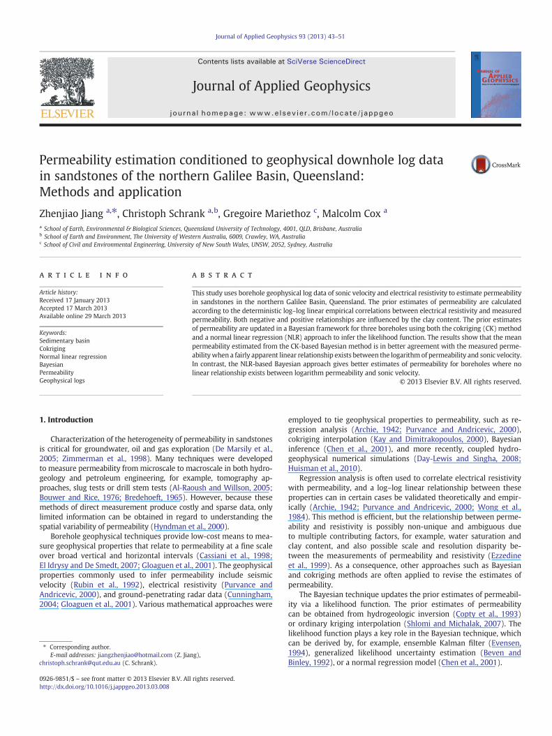
Fig. 1. Location map showing (a) the study area within the northern Galilee Basin, (b, c) bcolumn showing the general stratigraphy in the northern Galilee Basin.

steps are repeated until both the hydrogeologic and geophysical mea-surements fit well with the calculated results (Day-Lewis et al., 2003;Hinnell et al., 2010; Kowalsky et al., 2011; Pollock and Cirpka, 2012).

The accuracy of permeability estimated by the above methodsdepends on the sufficiency of actual permeability measurements. Inorder to overcome the problem of under-sampling in this study, theCK method is coupled with a Bayesian framework to calculate thelikelihood function. Both sonic and electrical log data are used toinfer the permeability in this coupled method, assuming that thecovariances of permeability and the resistivity are the same.

This study initially introduces the geology of the northern GalileeBasin, followed by a description of Bayesian framework and cokrigingtheory. The coupled CK–Bayesian method is then tested on threeboreholes in the northern Galilee Basin (Fig. 1). The performanceof the CK–Bayesian method is compared with another deterministicBayesian method based on normal linear regression. Finally, the mainresults are discussed.

2. Study area and data description

2.1. General geological setting

The Galilee Basin is a large intracratonic basin of the Late Carbon-iferous to Triassic period located in central Queensland, Australia(Fig. 1a). Sediments of the northern Galilee Basin were deposited intwo regional depressions, the Koburra Trough and Lovelle Depression,

oreholes with geophysical logs and permeability measurements, and (d) a schematic

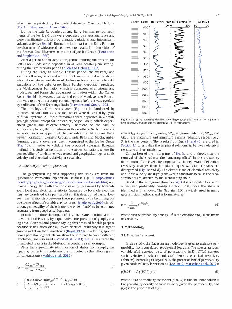
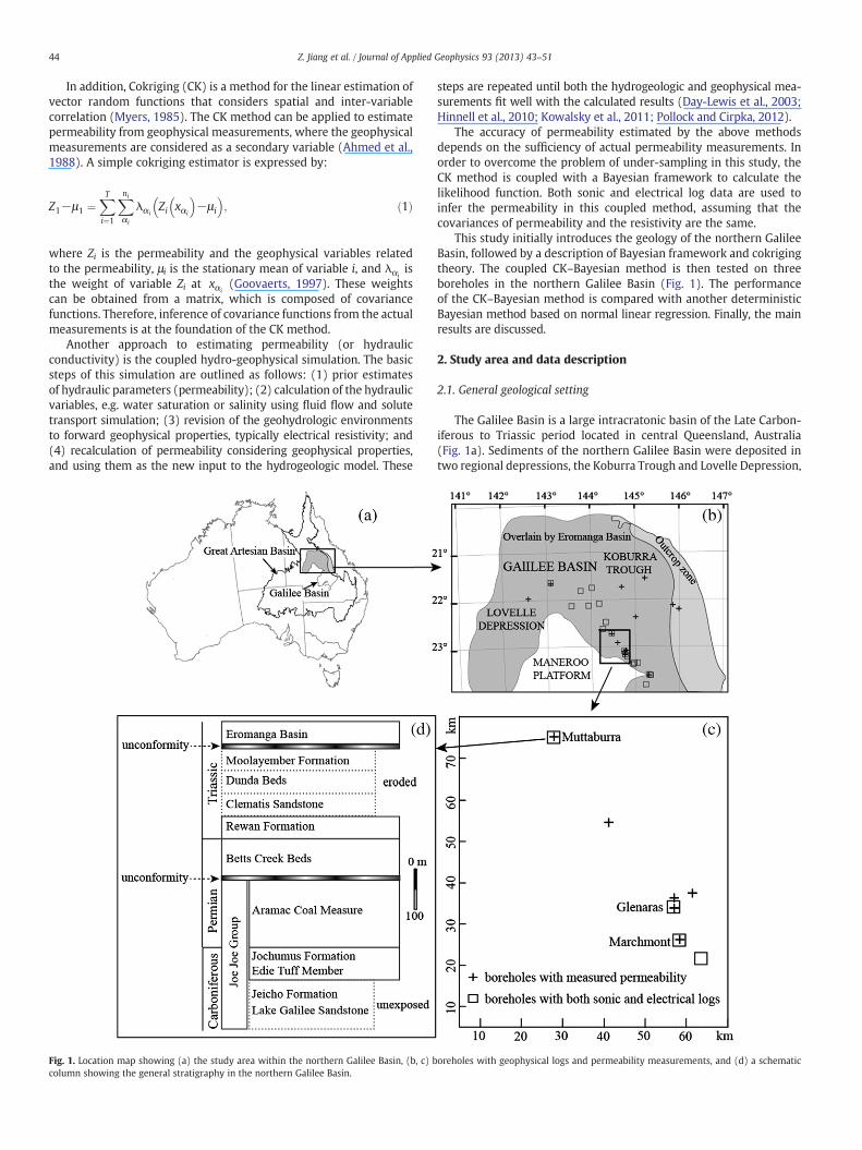
Fig. 2. Shales (grey rectangle) identified according to geophysical logs of natural gamma,deep resistivity and spontaneous potential (SP) in Muttaburra.

45Z. Jiang et al. / Journal of Applied Geophysics 93 (2013) 43–51

which are separated by the early Palaeozoic Maneroo Platform(Fig. 1b) (Hawkins and Green, 1993).

During the Late Carboniferous and Early Permian period, sedi-ments of the Joe Joe Group were deposited by rivers and lakes andwere significantly affected by climatic variations and intermittentvolcanic activity (Fig. 1d). During the latter part of the Early Permian,development of widespread peat swamps resulted in deposition ofthe Aramac Coal Measures at the top of Joe Joe Group (Hendersonand Stephenson, 1980).

After a period of non-deposition, gentle uplifting and erosion, theBetts Creek Beds were deposited in alluvial, coastal-plain settingsduring the Late Permian period (Allen and Fielding, 2007).

During the Early to Middle Triassic period, the westerly andsoutherly flowing rivers and intermittent lakes resulted in the depo-sition of sandstones and shales of the Rewan Formation and ClematisSandstone on the Betts Creek Beds. Further deposition producedthe Moolayember Formation which is composed of siltstones andmudstones and forms the uppermost formation within the GalileeBasin (Fig. 1d). However, a substantial part of Moolayember Forma-tion was removed in a compressional episode before it was overlainby sediments of the Eromanga Basin (Hawkins and Green, 1993).

The lithology of the study area (Fig. 1c) is dominated byinterbedded sandstones and shales, which were deposited by cyclicof fluvial systems. All these formations were deposited in a stablegeologic period, except for the earlier Joe Joe Group, which experi-enced glacial and volcanic activity. Therefore, on the basis ofsedimentary facies, the formations in this northern Galilee Basin areseparated into an upper part that includes the Betts Creek Beds,Rewan Formation, Clematis Group, Dunda Beds and MoolayemberFormation, and a lower part that is comprised of the Joe Joe Group(Fig. 1d). In order to validate the proposed cokriging–Bayesianmethod, this study concentrates on the upper formations where thepermeability of sandstones was tested and geophysical logs of sonicvelocity and electrical resistivity are available.

2.2. Data analysis and pre-processing

The geophysical log data supporting this study are from theQueensland Petroleum Exploration Database (QPED, http://mines.industry.qld.gov.au/geoscience/geoscience-wireline-log-data.htm) andExoma Energy Ltd. Both the sonic velocity (measured by boreholesonic logs) and electrical resistivity (acquired by borehole electricallogs) are correlated with permeability in this deep buried basin. How-ever, the relationship between these parameters can be ambiguousdue to the effects of variable clay contents (Friedel et al., 2006). In ad-dition, permeability of shale is too low (b10−3 mD) to be estimatedaccurately from geophysical log data.

In order to reduce the impact of clay, shales are identified and re-moved from this study by a qualitative interpretation of geophysicallog data. Electrical and gamma ray log data are used for this purposebecause shales often display lower electrical resistivity but highergamma radiation than sandstones (Kayal, 1979). In addition, sponta-neous potential logs which can show the interface between differentlithologies, are also used (Wood et al., 2003). Fig. 2 illustrates theinterpreted results in the Muttaburra borehole as an example.

After the approximate identification of shales from geophysicallogs, clay contents in sandstones are computed by the following em-pirical equations (Mahbaz et al., 2012):

IGR ¼ GR log−GRmin

GRmax−GRmin; ð2Þ

Sc ¼0:0006078 100IGRð Þ1:58257 IGRb0:552:1212IGR−0:81667 0:73 > IGR > 0:55IGR IGR > 0:73

;

8<: ð3Þ

where IGR is a gamma ray index, GRlog is gamma radiation, GRmin andGRmax are maximum and minimum gamma radiation, respectively.Sc is the clay content. The results from Eqs. (2) and (3) are used inSection 4.1 to establish the empirical relationship between electricalresistivity and permeability.

Comparison of the histograms of Fig. 3a and b shows that theremoval of shale reduces the “smearing effect” in the probabilitydistribution of sonic velocity. Importantly, the histogram of electricalresistivity changes from bimodal to quasi-Gaussian if shales aredisregarded (Fig. 3c and d). The distributions of electrical resistivityand sonic velocity are slightly skewed in sandstone because the mea-surements are affected by the surrounding shale.

Based on the histograms shown in Fig. 3, it is reasonable to assumea Gaussian probability density function (PDF) once the shale isidentified and removed. The Gaussian PDF is widely used in manygeostatistical methods, and is formulated as:

p ¼ 1ffiffiffiffiffiffiffiffiffiffiffiffi2πσ2

p e−Z xð Þ−μ½ �2

2σ2 ; ð4Þ

where p is the probability density, σ2 is the variance and μ is the meanof variable Z.

3. Methodology

3.1. Bayesian framework

In this study, the Bayesian methodology is used to estimate per-meability from correlated geophysical log data. The spatial randomvariable k(x) denotes log10 of permeability (mD), DT(x) denotessonic velocity (ms/feet), and ρ(x) denotes electrical resistivity(ohm-m). According to Bayes' rule, the posterior PDF of permeabilitygiven sonic velocity is written as (Lee, 2012; Mariethoz et al., 2010):

p k DTj Þ ¼ C⋅p DT kj Þ⋅p kð Þ;ðð ð5Þ

where C is a normalizing coefficient, p(DT|k) is the likelihood which isthe probability density of sonic velocity given the permeability, andp(k) is the prior PDF of k(x).

Fig. 3. Histograms of (a) sonic velocity and (c) log10-electrical resistivity measured in shales and sandstones in Muttaburra borehole at a separation of 0.2 m, (b) sonic velocity and(d) log10-electrical resistivity measured in sandstones at an average separation of 1.0 m.

46 Z. Jiang et al. / Journal of Applied Geophysics 93 (2013) 43–51

Since, by definition, ∫0∞p(k|DT)dk = 1, C can be calculated by

C ¼ 1

∫∞0p DT jkð Þ⋅p kð Þdk

: ð6Þ

The prior distribution of k is commonly estimated using an ordinarykriging approach based on the actual permeability measurements(Ezzedine et al., 1999; Shlomi andMichalak, 2007). However, the num-ber of actual permeability measurements in this study is not sufficientto quantify the covariance of permeability. Consequently, k cannotbe inferred by the ordinary kriging method. Alternatively, the priorestimates of permeability are calculated according to the empiricalrelationship between measured electrical resistivity and permeability.The details of this procedure are described in Sections 4.1 and 4.3.

The likelihood in Eq. (5) is assumed to follow a Gaussian distribu-tion (Eq. (4)). In this study, we use the cokriging method (CK) tocalculate the mean and variance of the likelihood. In order to validatethe effectiveness of the CK-based Bayesian method, the approachis compared with a normal linear regression (NLR) method for thecalculation of the likelihood.

3.2. Cokriging model

The CK algorithm considers the mean of likelihood at location xi asthe linear combination of first attributes DT(x) and second attributesk(x). All sonic velocity and prior estimates of permeability used aremean-removed and normalized by their global standard deviation.

This linear estimator of likelihood at xi can be written as (Goovaerts,1997):

μ xið Þ ¼Xj¼1j≠i

n1

λ1j xið ÞDT xj� �

þXn2j¼1

λ2j xið Þk xj� �

; ð7Þ

where, n1 and n2 are the number of DT and k measurements, respec-tively. λ1j and λ2j are the weighting coefficients of DT and k measure-ments at location xj. Because Eq. (7) is used to estimate the mean oflikelihood, it is allowed to be a biased estimator.

By minimizing the local variance at xi,

min : σ2 xið Þ ¼ E μ xið Þ−DT xið Þ½ �2; ð8Þ

where E denotes the mean operator. Subsequently, the coefficients λat location xi can be solved from the following equations:

Xw1¼1w1≠i

n1

λ1w1xið ÞC11 xv1−xw1

� �þ

Xn2w2¼1

λ2w2xið ÞC12 xv1−xw2

� �

¼ C11 xv1−xi� �

; v1 ¼ 1; ::i−1; iþ 1::n1

Xw1¼1w1≠i

n1

λ1w1xið ÞC21 xv2−xw1

� �þ

Xn2w2¼1

λ2w2xið ÞC22 xv2−xw2

� �

¼ C21 xv2−xi� �

; v2 ¼ 1; ::n2

ð9Þ

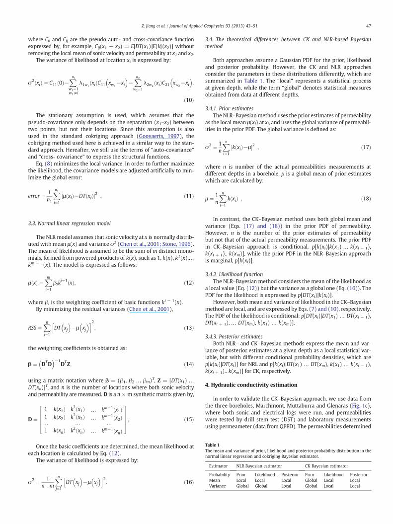
Table 1The mean and variance of prior, likelihood and posterior probability distribution in thenormal linear regression and cokriging Bayesian estimator.

Estimator NLR Bayesian estimator CK Bayesian estimator

Probability Prior Likelihood Posterior Prior Likelihood PosteriorMean Local Local Local Global Local LocalVariance Global Global Local Global Local Local

47Z. Jiang et al. / Journal of Applied Geophysics 93 (2013) 43–51

where Cii and Cij are the pseudo auto- and cross-covariance functionexpressed by, for example, Cij(x1 − x2) = E[DT(x1)]E(k[(x2)] withoutremoving the local mean of sonic velocity and permeability at x1 and x2.

The variance of likelihood at location xi is expressed by:

σ2 xið Þ ¼ C11 0ð Þ−Xw1¼1w1≠i

n1

λ1w1xið ÞC11 xw1

−xi� �

−Xn2

w2¼1

λ2w2xið ÞC21 xw2

−xi� �

:

ð10Þ

The stationary assumption is used, which assumes that thepseudo-covariance only depends on the separation (x1–x2) betweentwo points, but not their locations. Since this assumption is alsoused in the standard cokriging approach (Goovaerts, 1997), thecokriging method used here is achieved in a similar way to the stan-dard approach. Hereafter, we still use the terms of “auto-covariance”and “cross- covariance” to express the structural functions.

Eq. (8) minimizes the local variance. In order to further maximizethe likelihood, the covariance models are adjusted artificially to min-imize the global error:

error ¼ 1n1

Xn1i¼1

μ xið Þ−DT xið Þ½ �2 ; ð11Þ

3.3. Normal linear regression model

The NLRmodel assumes that sonic velocity at x is normally distrib-uted with mean μ(x) and variance σ2 (Chen et al., 2001; Stone, 1996).The mean of likelihood is assumed to be the sum of m distinct mono-mials, formed from powered products of k(x), such as 1, k(x), k2(x),…km − 1(x). The model is expressed as follows:

μ xð Þ ¼Xmi¼1

βiki−1 xð Þ; ð12Þ

where βi is the weighting coefficient of basic functions ki − 1(x).By minimizing the residual variances (Chen et al., 2001),

RSS ¼Xnj¼1

DT xj� �

−μ xj� �h i2

; ð13Þ

the weighting coefficients is obtained as:

β ¼ DTD� �−1

DTZ; ð14Þ

using a matrix notation where β = (β1, β2 … βm)T, Z = [DT(x1) …

DT(xn)]T, and n is the number of locations where both sonic velocityand permeability are measured. D is a n × m synthetic matrix given by,

D ¼1 k x1ð Þ k2 x1ð Þ … km−1 x1ð Þ1 k x2ð Þ k2 x2ð Þ … km−1 x2ð Þ… … …

1 k xnð Þ k2 xnð Þ … km−1 xnð Þ

26664

37775; ð15Þ

Once the basic coefficients are determined, the mean likelihood ateach location is calculated by Eq. (12).

The variance of likelihood is expressed by:

σ2 ¼ 1n−m

Xnj¼1

DT xj� �

−μ xj� �h i2

: ð16Þ

3.4. The theoretical differences between CK and NLR-based Bayesianmethod

Both approaches assume a Gaussian PDF for the prior, likelihoodand posterior probability. However, the CK and NLR approachesconsider the parameters in these distributions differently, which aresummarized in Table 1. The “local” represents a statistical processat given depth, while the term “global” denotes statistical measuresobtained from data at different depths.

3.4.1. Prior estimatesThe NLR–Bayesianmethod uses the prior estimates of permeability

as the local mean μ(xi) at xi, and uses the global variance of permeabil-ities in the prior PDF. The global variance is defined as:

σ2 ¼ 1n

Xni¼1

k xið Þ−μ½ �2 ; ð17Þ

where n is number of the actual permeabilities measurements atdifferent depths in a borehole, μ is a global mean of prior estimateswhich are calculated by:

μ ¼ 1n

Xni¼1

k xið Þ ; ð18Þ

In contrast, the CK–Bayesian method uses both global mean andvariance (Eqs. (17) and (18)) in the prior PDF of permeability.However, n is the number of the prior estimates of permeabilitybut not that of the actual permeability measurements. The prior PDFin CK–Bayesian approach is conditional, p[k(xi)|k(x1) … k(xi − 1),k(xi + 1).. k(xm)], while the prior PDF in the NLR–Bayesian approachis marginal, p[k(xi)].

3.4.2. Likelihood functionThe NLR–Bayesian method considers the mean of the likelihood as

a local value (Eq. (12)) but the variance as a global one (Eq. (16)). ThePDF for the likelihood is expressed by p[DT(xi)|k(xi)].

However, bothmean and variance of likelihood in the CK–Bayesianmethod are local, and are expressed by Eqs. (7) and (10), respectively.The PDF of the likelihood is conditional: p[DT(xi)|DT(x1) … DT(xi − 1),DT(xi + 1), … DT(xm), k(x1) … k(xm)].

3.4.3. Posterior estimatesBoth NLR– and CK–Bayesian methods express the mean and var-

iance of posterior estimates at a given depth as a local statistical var-iable, but with different conditional probability densities, which arep[k(xi)|DT(xi)] for NRL and p[k(xi)|DT(x1) … DT(xm), k(x1) … k(xi − 1),k(xi + 1).. k(xm)] for CK, respectively.

4. Hydraulic conductivity estimation

In order to validate the CK–Bayesian approach, we use data fromthe three boreholes, Marchmont, Muttaburra and Glenaras (Fig. 1c),where both sonic and electrical logs were run, and permeabilitieswere tested by drill stem test (DST) and laboratory measurementsusing permeameter (data from QPED). The permeabilities determined

Table 2The coefficients to calculate the likelihood functions.

Boreholes β1 β2 β3 β4 β5 β6

Marchmont 0.9754 1.2007 1.5734 0 0 0Muttaburra −1.5406 3.8752 −1.7358 0.0335 0 0Glenaras 0.5271 −0.3883 −2.0932 3.5008 −1.76532 0.2794

48 Z. Jiang et al. / Journal of Applied Geophysics 93 (2013) 43–51

from the geophysical data are calculated at a length scale of 1.0 m. Thelength scale of DST is around 0.5–2.0 m and that of cores ranges from0.1 to 0.5 m. Because these length scales are similar, permeabilitiesdetermined from these different methods are comparable. The effec-tiveness of the CK–Bayesian method is also compared with NLR–Bayesian method.

Permeability estimation with the CK– and NLR–Bayesian methodsentails the following steps: (1) estimation of prior PDF of permeabil-ity based on the electrical resistivity log data; (2) calculation of thelikelihood function using both the CK and NRL methods, respectively,where the likelihood function is the probability of permeabilityconditioned to the sonic log data; and (3) the posterior estimationof permeability based on Bayes' theorem in Eq. (5).

4.1. Prior estimation

Prior estimates of the permeability in sandstones are convertedfrom geoelectrical log data based on an experimental relationship.This relationship is established by mapping the measured perme-ability versus electrical resistivity measured at the same location.Fig. 4 illustrates that permeability (k) as a function of electrical resis-tivity (ρ) is affected by the clay content in upper formations of thenorth Galilee Basin. A negative correlation is observed betweenlog(k) and log(ρ) when the clay content is less than 5%; conversely,a positive correlation is obtained when the clay content is greaterthan 5%.

The electrical resistivity of earth materials relates to electrolytesin the pore fluid and electrons on the pore surface (Niwas andSinghal, 1985). In clay-free sandstone, the electrical current is dom-inated by electrical conduction through the pore fluid. An increase inporosity leads to an increase in permeability and thus to a decreasein electrical resistivity (Slater, 2007). Therefore, a negative trendis observed between ρ and k when no significant clay content ispresent.

However, in clay-rich sandstones, electrical current is controlledby electrical conduction on pore surfaces (Purvance and Andricevic,2000). Permeability commonly decreases with an increase in claycontent. The same trend exists between electrical resistivity andclay content when clay content is larger than 5%. Therefore, a positiverelationship between ρ and k is observed in clay-rich sandstones.

Based on the plots in Fig. 4, a bilinear experimental petrophysicalequation is given for sandstone formations in the northern GalileeBasin:

logk xð Þ ¼ −6:3753 logρ xð Þ þ 13:066 Sc b 5%1:8711 logρ xð Þ−2:5992 Sc > 5% ;

�ð19Þ

Although the permeability can be estimated from this bilinearrelationship, the low correlation coefficients (0.4091 and 0.3033,

Fig. 4. Scatterplots of (a) negative and positive linear relationships between log10-electricalbetween log10-electrical resistivity and clay content when clay content is larger than 5%. Ra

respectively) indicate large estimation errors. Therefore, the perme-ability estimated from this empirical equation is considered as priorestimate only. These results are then updated and improved via theBayesian framework.

4.2. Updating by Bayesian statistics

4.2.1. NLR-based estimationThe likelihood function plays a central role in Bayesian methods.

In the NLR approach, the mean and variance of the likelihood aredetermined by the coefficients of basic functions, which can be calcu-lated by Eq. (14) based on the actual measurements of permeabilityand sonic velocity. There are five such actual measurements inMarchmont borehole, six in Muttaburra and seven in Glenaras bore-holes. In a single borehole, these coefficients are considered to bespatially stationary at different depths. The resulting coefficients foreach borehole are shown in Table 2.

Once these coefficients are obtained, the mean and varianceof the likelihood at different depths are estimated by Eqs. (12)and (16), respectively. Consequently, the Gaussian PDF of the like-lihood is quantified by Eq. (4). Finally, the posterior estimates ofpermeability are obtained by Eq. (5) and results are shown inFig. 5a and c.

4.2.2. CK-based estimationThe CK approach assesses the mean and variance of the likelihood

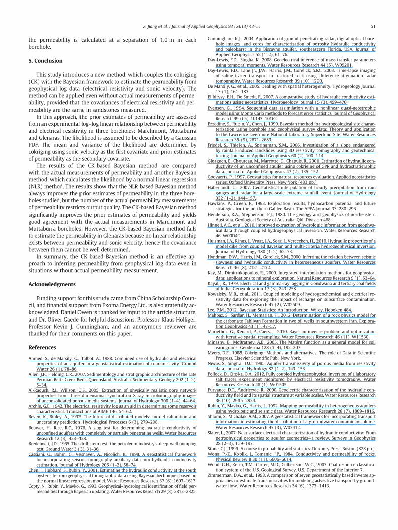
based on structural functions: auto- and cross- covariance. In thisstudy, the covariance of permeability is assumed to be the sameas the covariance of electrical resistivity after both are logarithm-transformed, mean-removed and normalized. This assumption issatisfied in this study because electrical resistivity and permeabilityare correlated linearly in each borehole (Fig. 4 and Eq. (19)). There-fore, the covariance of prior estimates of permeability can be usedto infer the likelihood via the CK algorithm. The covariances of theprior estimates of permeability and sonic velocity at different separa-tions (from 0 to 1000 m) are calculated and fitted using a sphericalcovariance model using the Matlab code variogramfit (Minasny andMcBratney, 2005).

resistivity and log10-permeability relating to clay content, and (b) negative relationshipw data are extracted from the Queensland Petroleum Exploration Database.

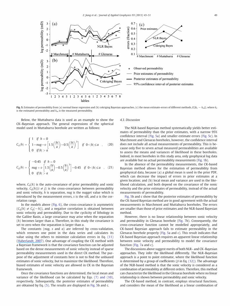
Fig. 5. Estimates of permeability from (a) normal linear regression and (b) cokriging Bayesian approaches, (c) the mean estimate-errors of different methods, E(|ke − km|), where keis the estimated permeability and km is the measured permeability.

49Z. Jiang et al. / Journal of Applied Geophysics 93 (2013) 43–51

Below, the Muttaburra data is used as an example to show theCK–Bayesian approach. The general expressions of the sphericalmodel used in Muttaburra borehole are written as follows:

Cii hð Þ ¼1 if h ¼ 0

1−nug−s⋅ 1:5hj ja

� �−0:5

hj ja

� �3� if 0b hj j≤a ;

0 if hj j > a

8>><>>:

ð20Þ

Cij hð Þ ¼−0:45 if h ¼ 0

nug þ s⋅ 1:5ha

� �−0:5

ha

� �3� −0:45 if 0b hj j≤a ;

0 if hj j > a

8>><>>:

ð21Þ

where, Cii(h) is the auto-covariance of prior permeability and sonicvelocity, Cij(h)(i ≠ j) is the cross-covariance between permeabilityand sonic velocity, h is separation, nug is the nugget value which isintroduced by the measurement errors, s is the sill, and a is the cor-relation range.

In the models above (Fig. 6), the cross-covariance is asymmetric(Cij(h) ≠ Cij(−h)), and a negative correlation is obtained betweensonic velocity and permeability. Due to the cyclicity of lithology inthe Galilee Basin, a large covariance may arise when the separation(h) becomes larger than a. Therefore, in this study the covariance isset to zero when the separation is larger than a.

The constants (nug, s and a) are inferred by cross-validation,which removes one point in the data series and calculates itsvalue using the others to minimize calculation errors in Eq. (11)(Haberlandt, 2007). One advantage of coupling the CK method witha Bayesian framework is that the covariance function can be adjustedbased on the dense measurements of sonic velocity instead of sparsepermeability measurements used in the direct CK method. The pur-pose of the adjustment of constants here is not to find the unbiasedestimates of sonic velocity, but to maximize the likelihood. Therefore,biased estimates of sonic velocity are allowed in CK in the Bayesianframework.

Once the covariance functions are determined, the local mean andvariance of the likelihood can be calculated by Eqs. (7) and (10),respectively. Subsequently, the posterior estimates of permeabilityare obtained by Eq. (5). The results are displayed in Fig. 5b and c.

4.3. Discussion

The NLR-based Bayesian method systematically yields better esti-mates of permeability than the prior estimates, with a narrow 95%confidence interval (Fig. 5a) and smaller estimate errors (Fig. 5c). InMarchmont and Glenaras boreholes, however, the confidence intervaldoes not include all actual measurements of permeability. This is be-cause only five to seven actual measured permeabilities are availableto assess the means and variances of likelihood in these boreholes.Indeed, in most boreholes in this study area, only geophysical log dataare available but no actual permeability measurements (Fig. 1b).

In the absence of the permeability measurements, the CK-basedBayesian method allows for the estimation of permeability fromgeophysical data, because (a) a global mean is used in the prior PDF,which can decrease the impact of errors in prior estimates at agiven location; and (b) local mean and variance are used in the like-lihood calculation, and both depend on the covariance of the sonicvelocity and the prior estimates of permeability, instead of the actualmeasurements of permeability.

Fig. 5b and c show that the posterior estimates of permeability bythe CK-based Bayesian method are in good agreement with the actualmeasurements in Marchmont and Muttaburra boreholes. The errorsare smaller than those of prior estimates and the NLR-based Bayesianmethod.

However, there is no linear relationship between sonic velocityand permeability in Glenaras borehole (Fig. 7b). Consequently, thecross-covariance function cannot be modelled appropriately, andCK-based Bayesian approach fails to estimate permeability in theGlenaras borehole properly (Fig. 5a and c). This result indicates thatCK-based Bayesian approach requires an apparent linear relationshipbetween sonic velocity and permeability to model the covariancefunction (Fig. 7a and c).

The discussions above suggestmerits of bothNLR– and CK–Bayesianapproaches. They infer the likelihood differently. The NLR–Bayesianapproach is a point to point estimator, where the likelihood functionis determined by a group of coefficients (β in Eq. (12)). The advantageof the NLR-based method is that the sonic velocity is considered as acombination of permeability at different orders. Therefore, this methodcan characterize the likelihood in theGlenaras boreholewhere no linearrelationship is shown between permeability and sonic velocity.

The CK-based method, in contrast, employs structural functions,and considers the mean of the likelihood as a linear combination of

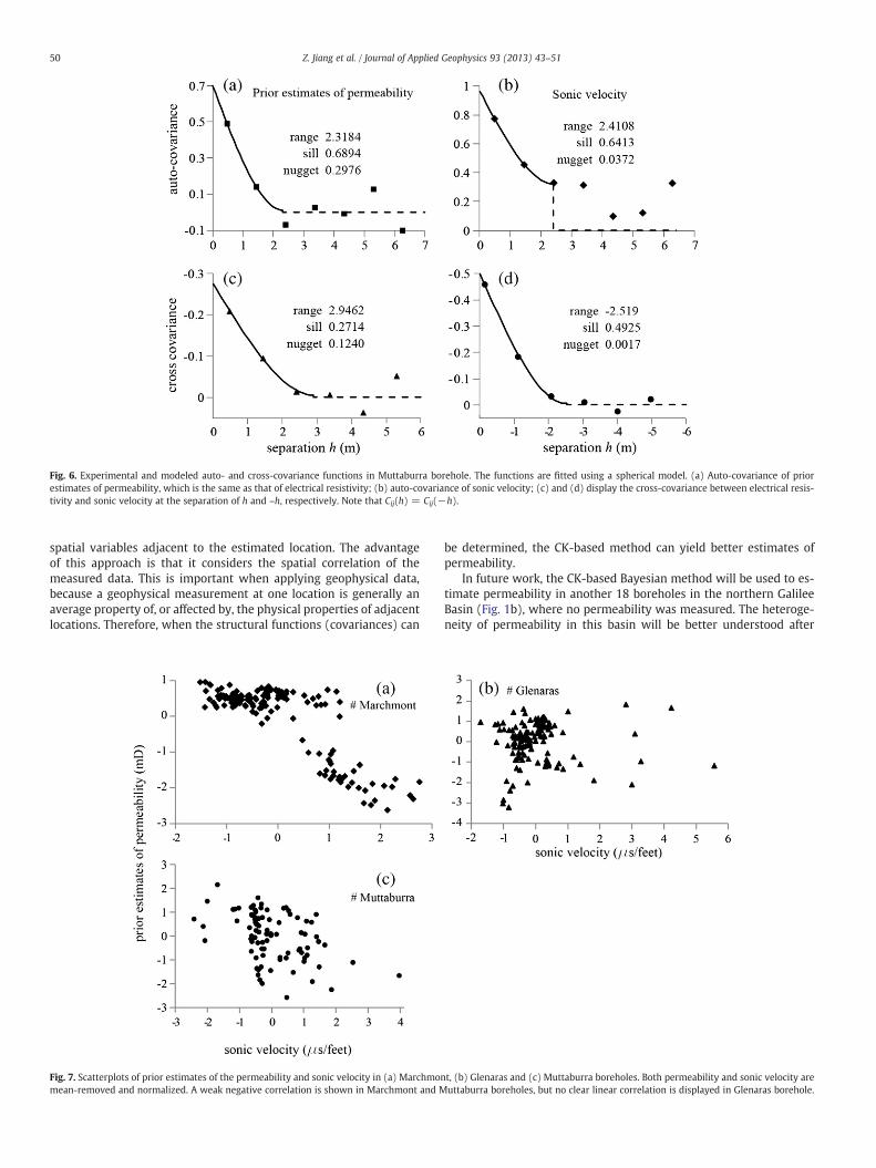
Fig. 6. Experimental and modeled auto- and cross-covariance functions in Muttaburra borehole. The functions are fitted using a spherical model. (a) Auto-covariance of priorestimates of permeability, which is the same as that of electrical resistivity; (b) auto-covariance of sonic velocity; (c) and (d) display the cross-covariance between electrical resis-tivity and sonic velocity at the separation of h and –h, respectively. Note that Cij(h) = Cij(−h).

50 Z. Jiang et al. / Journal of Applied Geophysics 93 (2013) 43–51

spatial variables adjacent to the estimated location. The advantageof this approach is that it considers the spatial correlation of themeasured data. This is important when applying geophysical data,because a geophysical measurement at one location is generally anaverage property of, or affected by, the physical properties of adjacentlocations. Therefore, when the structural functions (covariances) can

Fig. 7. Scatterplots of prior estimates of the permeability and sonic velocity in (a) Marchmonmean-removed and normalized. A weak negative correlation is shown in Marchmont and M

be determined, the CK-based method can yield better estimates ofpermeability.

In future work, the CK-based Bayesian method will be used to es-timate permeability in another 18 boreholes in the northern GalileeBasin (Fig. 1b), where no permeability was measured. The heteroge-neity of permeability in this basin will be better understood after

t, (b) Glenaras and (c) Muttaburra boreholes. Both permeability and sonic velocity areuttaburra boreholes, but no clear linear correlation is displayed in Glenaras borehole.

51Z. Jiang et al. / Journal of Applied Geophysics 93 (2013) 43–51

the permeability is calculated at a separation of 1.0 m in eachborehole.

5. Conclusion

This study introduces a new method, which couples the cokriging(CK) with the Bayesian framework to estimate the permeability fromgeophysical log data (electrical resistivity and sonic velocity). Themethod can be applied even without actual measurements of perme-ability, provided that the covariances of electrical resistivity and per-meability are the same in sandstones measured.

In this approach, the prior estimates of permeability are assessedfrom an experimental log–log linear relationship between permeabilityand electrical resistivity in three boreholes: Marchmont, Muttaburraand Glenaras. The likelihood is assumed to be described by a GaussianPDF. The mean and variance of the likelihood are determined bycokriging using sonic velocity as the first covariate and prior estimatesof permeability as the secondary covariate.

The results of the CK-based Bayesian method are comparedwith the actual measurements of permeability and another Bayesianmethod, which calculates the likelihood by a normal linear regression(NLR) method. The results show that the NLR-based Bayesian methodalways improves the prior estimates of permeability in the three bore-holes studied, but the number of the actual permeabilitymeasurementsof permeability restricts output quality. The CK-based Bayesianmethodsignificantly improves the prior estimates of permeability and yieldsgood agreement with the actual measurements in Marchmont andMuttaburra boreholes. However, the CK-based Bayesian method failsto estimate the permeability in Glenaras because no linear relationshipexists between permeability and sonic velocity, hence the covariancebetween them cannot be well determined.

In summary, the CK-based Bayesian method is an effective ap-proach to inferring permeability from geophysical log data even insituations without actual permeability measurement.

Acknowledgments

Funding support for this study came from China Scholarship Coun-cil, and financial support from Exoma Energy Ltd. is also gratefully ac-knowledged. Daniel Owen is thanked for input to the article structure,and Dr. Oliver Gaede for helpful discussions. Professor Klaus Holliger,Professor Kevin J. Cunningham, and an anonymous reviewer arethanked for their comments on this paper.

References

Ahmed, S., de Marsily, G., Talbot, A., 1988. Combined use of hydraulic and electricalproperties of an aquifer in a geostatistical estimation of transmissivity. GroundWater 26 (1), 78–86.

Allen, J.P., Fielding, C.R., 2007. Sedimentology and stratigraphic architecture of the LatePermian Betts Creek Beds, Queensland, Australia. Sedimentary Geology 202 (1–2),5–34.

Al-Raoush, R.I., Willson, C.S., 2005. Extraction of physically realistic pore networkproperties from three-dimensional synchrotron X-ray microtomography imagesof unconsolidated porous media systems. Journal of Hydrology 300 (1–4), 44–64.

Archie, G.E., 1942. The electrical resistivity log as an aid in determining some reservoircharacteristics. Transactions of AIME 146, 54–62.

Beven, K., Binley, A., 1992. The future of distributed models: model calibration anduncertainty prediction. Hydrological Processes 6 (3), 279–298.

Bouwer, H., Rice, R.C., 1976. A slug test for determining hydraulic conductivity ofunconfined aquifers with completely or partially penetrating wells. Water ResourcesResearch 12 (3), 423–428.

Bredehoeft, J.D., 1965. The drill-stem test: the petroleum industry's deep-well pumpingtest. Ground Water 3 (3), 31–36.

Cassiani, G., Böhm, G., Vesnaver, A., Nicolich, R., 1998. A geostatistical frameworkfor incorporating seismic tomography auxiliary data into hydraulic conductivityestimation. Journal of Hydrology 206 (1–2), 58–74.

Chen, J., Hubbard, S., Rubin, Y., 2001. Estimating the hydraulic conductivity at the southoyster site from geophysical tomographic data using Bayesian techniques based onthe normal linear regression model. Water Resources Research 37 (6), 1603–1613.

Copty, N., Rubin, Y., Mavko, G., 1993. Geophysical–hydrological identification of field per-meabilities through Bayesian updating.Water Resources Research 29 (8), 2813–2825.

Cunningham, K.J., 2004. Application of ground-penetrating radar, digital optical bore-hole images, and cores for characterization of porosity hydraulic conductivityand paleokarst in the Biscayne aquifer, southeastern Florida, USA. Journal ofApplied Geophysics 55 (1–2), 61–76.

Day-Lewis, F.D., Singha, K., 2008. Geoelectrical inference of mass transfer parametersusing temporal moments. Water Resources Research 44 (5), W05201.

Day-Lewis, F.D., Lane Jr., J.W., Harris, J.M., Gorelick, S.M., 2003. Time-lapse imagingof saline-tracer transport in fractured rock using difference-attenuation radartomography. Water Resources Research 39 (10), 1290.

De Marsily, G., et al., 2005. Dealing with spatial heterogeneity. Hydrogeology Journal13 (1), 161–183.

El Idrysy, E.H., De Smedt, F., 2007. A comparative study of hydraulic conductivity esti-mations using geostatistics. Hydrogeology Journal 15 (3), 459–470.

Evensen, G., 1994. Sequential data assimilation with a nonlinear quasi-geostrophicmodel using Monte Carlo methods to forecast error statistics. Journal of GeophysicalResearch 99 (C5), 10143–10162.

Ezzedine, S., Rubin, Y., Chen, J., 1999. Bayesian method for hydrogeological site charac-terization using borehole and geophysical survey data: Theory and applicationto the Lawrence Livermore National Laboratory Superfund Site. Water ResourcesResearch 35 (9), 2671–2683.

Friedel, S., Thielen, A., Springman, S.M., 2006. Investigation of a slope endangeredby rainfall-induced landslides using 3D resistivity tomography and geotechnicaltesting. Journal of Applied Geophysics 60 (2), 100–114.

Gloaguen, E., Chouteau, M., Marcotte, D., Chapuis, R., 2001. Estimation of hydraulic con-ductivity of an unconfined aquifer using cokriging of GPR and hydrostratigraphicdata. Journal of Applied Geophysics 47 (2), 135–152.

Goovaerts, P., 1997. Geostatistics for natural resources evaluation. Applied geostatisticsseries. Oxford University Press, New York (483 pp.).

Haberlandt, U., 2007. Geostatistical interpolation of hourly precipitation from raingauges and radar for a large-scale extreme rainfall event. Journal of Hydrology332 (1–2), 144–157.

Hawkins, P., Green, P., 1993. Exploration results, hydrocarbon potential and futurestrategies for the northern Galilee Basin. The APEA Journal 33, 280–296.

Henderson, R.A., Stephenson, P.J., 1980. The geology and geophysics of northeasternAustralia. Geological Society of Australia, Qld. Division 468.

Hinnell, A.C., et al., 2010. Improved extraction of hydrologic information from geophys-ical data through coupled hydrogeophysical inversion. Water Resources Research46, W00D40.

Huisman, J.A., Rings, J., Vrugt, J.A., Sorg, J., Vereecken, H., 2010. Hydraulic properties of amodel dike from coupled Bayesian and multi-criteria hydrogeophysical inversion.Journal of Hydrology 380 (1–2), 62–73.

Hyndman, D.W., Harris, J.M., Gorelick, S.M., 2000. Inferring the relation between seismicslowness and hydraulic conductivity in heterogeneous aquifers. Water ResourcesResearch 36 (8), 2121–2132.

Kay, M., Dimitrakopoulos, R., 2000. Integrated interpolation methods for geophysicaldata: applications to mineral exploration. Natural Resources Research 9 (1), 53–64.

Kayal, J.R., 1979. Electrical and gamma-ray logging in Gondwana and tertiary coal fieldsof India. Geoexploration 17 (3), 243–258.

Kowalsky, M.B., et al., 2011. Coupled modeling of hydrogeochemical and electrical re-sistivity data for exploring the impact of recharge on subsurface contamination.Water Resources Research 47 (2), W02509.

Lee, P.M., 2012. Bayesian Statistics: An Introduction. Wiley, Hoboken 484.Mahbaz, S., Sardar, H., Memarian, H., 2012. Determination of a rock physics model for

the carbonate Fahliyan Formation in two oil wells in southwestern Iran. Explora-tion Geophysics 43 (1), 47–57.

Mariethoz, G., Renard, P., Caers, J., 2010. Bayesian inverse problem and optimizationwith iterative spatial resampling. Water Resources Research 46 (11), W11530.

Minasny, B., McBratney, A.B., 2005. The Matérn function as a general model for soilvariograms. Geoderma 128 (3–4), 192–207.

Myers, D.E., 1985. Cokriging: Methods and alternatives. The role of Data in ScientificProgress. Elsevier Scientific Pub., New York.

Niwas, S., Singhal, D.C., 1985. Aquifer transmissivity of porous media from resistivitydata. Journal of Hydrology 82 (1–2), 143–153.

Pollock, D., Cirpka, O.A., 2012. Fully coupled hydrogeophysical inversion of a laboratorysalt tracer experiment monitored by electrical resistivity tomography. WaterResources Research 48 (1), W01505.

Purvance, D.T., Andricevic, R., 2000. Geoelectric characterization of the hydraulic con-ductivity field and its spatial structure at variable scales. Water Resources Research36 (10), 2915–2924.

Rubin, Y., Mavko, G., Harris, J., 1992. Mapping permeability in heterogeneous aquifersusing hydrologic and seismic data. Water Resources Research 28 (7), 1809–1816.

Shlomi, S., Michalak, A.M., 2007. A geostatistical framework for incorporating transportinformation in estimating the distribution of a groundwater contaminant plume.Water Resources Research 43 (3), W03412.

Slater, L., 2007. Near surface electrical characterization of hydraulic conductivity: Frompetrophysical properties to aquifer geometries—a review. Surveys in Geophysics28 (2–3), 169–197.

Stone, C.J., 1996. A course in probability and statistics. Duxbury Press, Boston (828 pp.).Wong, P.-Z., Koplik, J., Tomanic, J.P., 1984. Conductivity and permeability of rocks.

Physical Review B 30 (11), 6606–6614.Wood, G.H., Kehn, T.M., Carter, M.D., Culbertson, W.C., 2003. Coal resource classifica-

tion system of the U.S. Geological Survey. U.S. Department of the Interior 7.Zimmerman, D.A., et al., 1998. A comparison of seven geostatistically based inverse ap-

proaches to estimate transmissivities for modeling advective transport by ground-water flow. Water Resources Research 34 (6), 1373–1413.