Performance Analysis of Existing and New

Methods for Data Hiding with Known-Host

Information in Additive Channels

Fernando Perez-Gonzalez†, Member, IEEE, Felix Balado† and Juan R. Hernandez‡

EDICS Category: 5–AUTH

Work partially funded by the Xunta de Galicia under projects PGIDT01 PX132204PM and PGIDT02 PXIC32205PN,

the European project Certimark (Certification of Watermarking Technologies), IST-1999-10987, and the CYCIT project

AMULET, reference TIC2001-3697-C03-01.

† Dept. Teorıa de la Senal y Comunicaciones, ETSI Telecom., Universidad de Vigo, 36200 Vigo, Spain

‡ Lysis SA, Cotes de Montbenon 8, 1004 Lausanne, Switzerland

E-mails: fperez@tsc.uvigo.es, fiz@tsc.uvigo.es, juan-ramon.hernandez@nagra.com

November 18, 2002 DRAFT

1

Abstract

A considerable amount of attention has been lately payed to a number of data hiding methods based in

quantization, seeking to achieve in practice the results predicted by Costa for a channel with side information at

the encoder. With the objective of filling a gap in the literature, this paper supplies a fair comparison between

significant representatives of both this family of methods and the former spread-spectrum approaches that make

use of near-optimal ML decoding; the comparison is based on measuring their probabilities of decoding error

in the presence of channel distortions. Accurate analytical expressions and tight bounds for the probability of

decoding error are given and validated by means of Monte Carlo simulations. For Dithered Modulation (DM)

a novel technique that allows to obtain tighter bounds to the probability of error is presented. Within the new

framework, the strong points and weaknesses of both methods are distinctly displayed. This comparative study

allows us to propose a new technique named “Quantized Projection” (QP), which by adequately combining

elements of those previous approaches, produces gains in performance.

I. Introduction

Data hiding is the generic name given to a number of techniques having the common characteristic of

inserting a certain set of data into a regular signal without noticeably modifying it. The growing amount

of exchanged information since the expansion of the Internet during the last decade has motivated an

active and prolific research in this field. It has also focused the attention of the investigations on

multimedia signals (i.e. image, video and audio) as typical host signals for carrying the hidden data.

The kind of multimedia applications of data hiding ranges from steganography, where the sheer act

of the embedment tries to be concealed, to copyright enforcement and/or fingerprinting, where the

hidden information has to reliably identify the host signal and/or its legal owner even under tampering

efforts. The requirements for these applications also vary considerably. One of the most elusive of

these requirements has been, since the first attempts, robustness, i.e. the ability to survive intentional

or unintentional attacks aiming at removing or modifying the embedded payload.

Although a young discipline, digital data hiding has already gone through two different phases.

During the first one, algorithms flooded the literature, in most cases with weak theoretical grounds

and with little concern about robustness or performance [1], [2]. The second phase started with

the recognition that the data hiding problem was in fact a particular case of communications [3],

clearing the way for using well-known techniques, such as spread-spectrum, and facilitating subsequent

performance analyses. Also, researchers started to look at data hiding under the light of information

theory, thus helping to establish fundamental limits on performance. Within this framework the

November 18, 2002 DRAFT

2

problem of embedding can be assimilated to optimally encoding the information to be hidden by shaping

the host signal under certain perceptual restrictions; next, this signal goes through a statistical channel

representing the eventual attacks before arriving to the decoder, which tries to recover the embedded

information from the channel output as reliably as possible.

A third and current phase started when Cox et al. [4] identified that the data hiding problem could

in addition be seen as one of communications with side information at the encoder. Soon afterwards,

an important result by Costa [5] was rescued by Chen and Wornell in [6]. In his paper, Costa gave

a solution for obtaining null host signal interference for a known realization of a Gaussian host signal

and a random Gaussian channel. Then, the problem with side information only at the encoder —

usually termed as “blind” data hiding— could be seen as equivalent to having full side information at

the decoder. A number of down-to-earth implementations aiming at practically approaching Costa’s

construction have sprung since then [6], [7], [8], consisting in most cases in quantization procedures.

This family of approaches, that from now on will be referred to as known-host-state methods, has

been claimed to improve the performance of those usually called “spread spectrum” [3], [9] which use

different forms of diversity. In principle, the latter do not make use of host signal state information,

although they are not completely unaware of it as most of them utilize the host state for determining

the maximum allowed perceptual distortion. Moreover, in their best performing versions they employ

statistical information about the host signal to construct optimal or near-optimal detectors. This

usage of host signal statistics in their detection algorithms permits us to denominate them known-

host-statistics methods.

The first objective of this paper is to provide a fair and rigorous comparison of the performance

yielded by some of the most important representatives of these two families of methods, which is lacking

in the literature. Some previous analyses rely on questionable assumptions and/or simplifications, that

we will try to overcome. A further motivation for revisiting some recently proposed methods leans

on the fact that Costa’s scheme is only optimal for a certain class of channels and host signals. In

fact, we will show that, as it frequently happens with real world communications systems, channel

capacity, important as it is, becomes secondary to other performance measurements, such as the bit

error probability. We will see that, since known-host-state methods do not use host signal information

in their detection procedures —i.e. detectors act in a “deterministic” fashion—, in certain cases they

happen to be too sensitive to certain power-limited channel distortions. On the other hand, even

though known-host-statistics methods do present the so-called host signal interference (meaning that

a zero probability of decoding error is not attainable), we will verify that in some cases they prove to

November 18, 2002 DRAFT

3

be robust enough to better withstand such channel perturbations. All considered, this suggests that

there may exist better practical approaches that encompass both watermarking philosophies, i.e. the

use of channel state information together with host signal statistics information. This door was already

opened by Chen and Wornell who proposed the idea of “spreading” known-host-state schemes (Spread

Transforms), much in the same way as additive spread spectrum schemes improve its operating signal-

to-noise ratio (SNR) [10]. In this paper, we will propose a variant called Quantized Projection, which

will be analyzed from the perspective of its probability of bit error, providing accurate formulas for

its computation and showing how computationally attractive choices of the parameters offer excellent

performance and robustness in front of channel distortions.

The paper is organized as follows. In Sect. II the basic definitions and conventions are formulated.

Next, in Sects. III and IV we analyze the behavior of some of the most representative known-host-state

and known-host-statistics methods under channel distortions. The conclusions serve us to propose

in Sect. V the Quantized Projection scheme, which we demonstrate improves the former methods.

Last we compare the empirical and predicted probabilities of decoding error of all of these methods in

Sect. VI and we draw the final conclusions in Sect. VII.

II. Problem formulation

We will restrict our analysis to data hiding in still images, as most of the prevalent algorithms have

taken this kind of host signals for benchmarking purposes. The model that we will follow is summarized

in Figure 1. Let x be a vector containing the samples of the host signal that will convey the hidden

information; these vector samples are taken in a certain domain of interest that we will discuss later.

We will make the hypothesis that x[k] is a zero-mean random variable (r.v.); should this not be true,

the exposition would remain valid after subtracting the non-zero mean from x[k]. Before the encoding

stage, a perceptual mask vector α is computed from x in the appropriate domain, taking into account

the characteristics of the Human Visual System (HVS) and indicating the maximum allowed energy

that produces the least noticeable modification of the corresponding sample from the host signal. Next,

using a cryptographic key K, a watermark w is produced from the desired binary information vector

b using a certain function, w = gK(x,α,b). Without loss of generality we will write the watermarked

signal as the addition y = x + w. (Fig. 1

goes

here)In the sequel we will concentrate only on the problem of hidden information decoding rather than

watermark detection, and we will use the decoding bit error probability (Pe) as the final performance

November 18, 2002 DRAFT

4

measurement. Other performance indices such as the signal-to-noise ratio (SNR) [6], [10] or the mutual

information [7] between the sent message and the channel output have also been proposed. Nevertheless

we feel that, in the data hiding problem, the probability of decoding error is the most reasonable

measurement for comparing two methods. First, as it will be further developed throughout this paper,

different SNR’s might eventually lead to the same value of Pe under different underlying statistical

models for the host signal. Second, the mutual information measurement just establishes an upper

bound on the admissible rate, that can usually be achieved only under certain ideal conditions.

We will also assume that we want to hide only one binary digit of information b that we consider to

be mapped to an antipodal symbol, b ∈ {±1}. Two cases will be addressed:

• Unidimensional case, where only one host signal sample x[k] is used to convey the information bit.

Although not very practical by itself due to the high Pe associated, this case is interesting because it

reveals the underlying mechanisms that appear when many dimensions are used.

• Multidimensional case, in which the information bit is embedded using a set S = {k1, . . . , k|S|} of

key-dependent pseudorandomly chosen indices selecting L = |S| samples from x. Obviously, in this

case the obtained results will depend on the partition S and should be averaged over all possible

partitions for a given host signal (see [11]). In this paper this averaging is not undertaken because for

comparison purposes it is sufficient to consider a single partition.

It is also important to observe that in the multidimensional case no form of coding other than

repetition will be considered. As this paper targets at the comparison of several families of methods, it

is out of its scope the consideration of better coding strategies, which are of course possible, as it has

been shown in previous literature [11]. Thus, repetition coding can be regarded as the simplest way of

achieving the necessary gain for the data hiding problem (for which the SNR is very low) and serves

as a baseline for the comparison of ‘raw’ algorithms. Moreover, repetition (or, equivalently, spreading)

is very well-suited against attacks such as cropping. We will see the effect of this kind of coding with

the appearance of a factor√

L (repetition coding gain) governing the asymptotic performance of the

multidimensional analyses. Since increasing the size L of the embedding set will always reduce the

probability of error, the actual choice of L will be only limited by the ratio between the number of

available samples and the amount of payload to be hidden.

November 18, 2002 DRAFT

5

A. Embedding distortion

A crucial aspect when performing a rigorous analysis lies in the election of proper distortion measures.

Let us consider first the issue of embedding distortion. We will adhere to the often used global Mean-

Squared Error (MSE) distortion [12], [10], which for the single bit case is defined as

Dw =1L

∑k∈S

E{w2[k]},

where w[k] is a random process representing the watermark. A straightforward generalization of this

definition is possible for the multibit case.

The MSE, being adequate for measuring the total power devoted to the watermark, should be handled

with care when dealing with visibility constraints. Although just constraining Dw to remain below a

certain level is very convenient from an analytical point of view (e.g., Costa’s result was enunciated for

this type of restriction), it is at the same time questionable for the purpose of data hiding in images,

because it is not well-matched to the characteristics of the HVS, as explicitly mentioned in [12]. It

is widely recognized that the masking phenomena affecting the HVS and exploited for the invisible

embedment of information respond to local effects. All existing approaches to modeling distortions

which are unnoticeable to the HVS take into account this fact, be it the Just Noticeable Distortion

function (JND) [13] in the spatial domain, the Noise Visibility Function (NVF) [14] applicable to

different domains, or equivalent models in other domains of interest like the DCT.

The main drawback encountered is that unacceptably high local distortions (from the perceptual

perspective) could be globally compensated to meet the established restriction. An alternative consist-

ing in a weighted MSE is discussed in [12]. This type of distortion measurement is appropriate when

the weighting refers to local neighborhoods of the signal, e.g. sub-bands in a frequential transform or

vicinities in spatial coordinates. In the extreme case, these neighborhoods consist only of one element

and the weighted MSE criterion is formally equivalent to the samplewise one, which is discussed below.

In view of the discussion above, it seems reasonable to constrain the local variance of the watermark

in such a way that global compensations are not possible and at the same time perceptual weighting

is taken into account. This is achieved by means of the following set of constraints:

E{w2[k]} ≤ α2[k], ∀ k ∈ S, (1)

where the α[k] account for the perceptual characteristics of the HVS and ideally are determined so as

to produce the least visible impact for a certain watermark energy. Note that if the pseudorandom

November 18, 2002 DRAFT

6

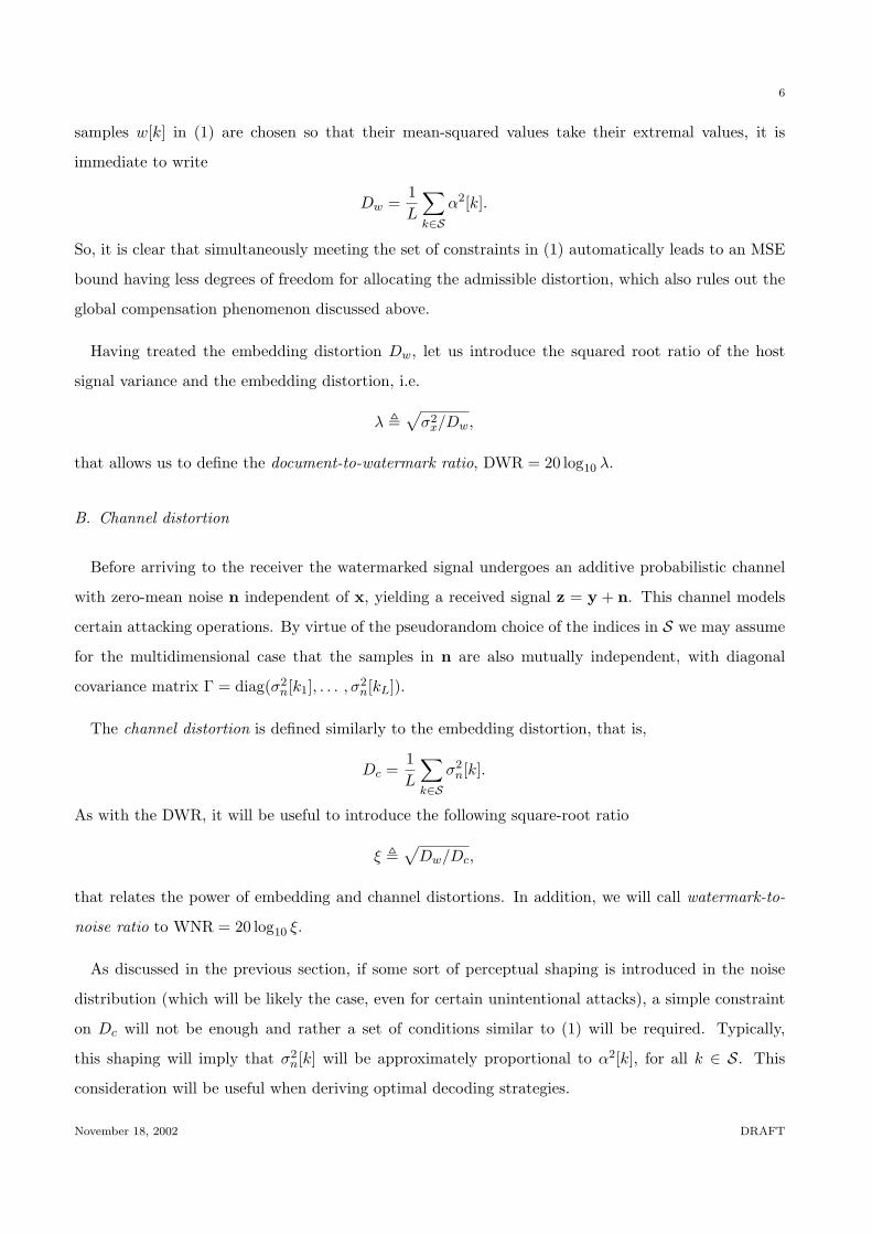
samples w[k] in (1) are chosen so that their mean-squared values take their extremal values, it is

immediate to write

Dw =1L

∑k∈S

α2[k].

So, it is clear that simultaneously meeting the set of constraints in (1) automatically leads to an MSE

bound having less degrees of freedom for allocating the admissible distortion, which also rules out the

global compensation phenomenon discussed above.

Having treated the embedding distortion Dw, let us introduce the squared root ratio of the host

signal variance and the embedding distortion, i.e.

λ ,√

σ2x/Dw,

that allows us to define the document-to-watermark ratio, DWR = 20 log10 λ.

B. Channel distortion

Before arriving to the receiver the watermarked signal undergoes an additive probabilistic channel

with zero-mean noise n independent of x, yielding a received signal z = y + n. This channel models

certain attacking operations. By virtue of the pseudorandom choice of the indices in S we may assume

for the multidimensional case that the samples in n are also mutually independent, with diagonal

covariance matrix Γ = diag(σ2n[k1], . . . , σ2

n[kL]).

The channel distortion is defined similarly to the embedding distortion, that is,

Dc =1L

∑k∈S

σ2n[k].

As with the DWR, it will be useful to introduce the following square-root ratio

ξ ,√

Dw/Dc,

that relates the power of embedding and channel distortions. In addition, we will call watermark-to-

noise ratio to WNR = 20 log10 ξ.

As discussed in the previous section, if some sort of perceptual shaping is introduced in the noise

distribution (which will be likely the case, even for certain unintentional attacks), a simple constraint

on Dc will not be enough and rather a set of conditions similar to (1) will be required. Typically,

this shaping will imply that σ2n[k] will be approximately proportional to α2[k], for all k ∈ S. This

consideration will be useful when deriving optimal decoding strategies.

November 18, 2002 DRAFT

7

It is difficult to answer the question of what choice of the probability distribution function (pdf) of

the distortion, under a restriction on its variance, causes the worst Pe on the receiver. In general, it

will heavily depend upon both the embedding and detection methods employed. The Gaussian channel

has been commonly used in previous analyses of known-host-state data hiding schemes [10], [7] as a

reference for measuring system performance; one argument supporting this choice is that Gaussian

channel models can be expected to be good for a variety of applications in which robustness against

unintentional attacks is required [10]. Also in [15] it is remarked that the additive white Gaussian

noise channel is of interest because it can be easily applied to any watermarking method, giving

upper capacity bounds to a more general scenario. In addition it has been shown in [16] that, under

the assumption of a Gaussian host signal, the Gaussian channel is the optimal attack under MSE

distortion restrictions. For all these reasons we will consider this type of distortion in our analysis.

However, we will also show how a simple uniform pdf can sometimes cause more harm to the

performance of certain methods than Gaussian noise with the same variance. There are three reasons

for also choosing this pdf: first, it leads in many cases to tractable analytical expressions of performance

that permit to gain insight into the behavior of the algorithms; second, we will show that it can be an

especially harmful attack to some of the algorithms analyzed, as many of the existing known-host-state

methods are based on uniform quantizers. Last, this kind of noise is unintentionally present whenever

the watermarked signal is finely quantized (or requantized) [17].

C. Modeling

In Section IV we will assume that the host signal x is defined in the DCT (discrete cosine transform)

domain since a statistical model will be necessary. The reason for the election of this domain is

twofold: first, since good statistical models are available for the elements of x, it is possible to arrive

at a complete theoretical formulation of the problem that will allow a fair comparison between the

different classes of algorithms; second, the DCT has important practical implications (for instance, it

is used in the JPEG standard). Consequently, the perceptual mask will be computed in this domain.

The details into the calculation of such mask were given in [18].

III. Known-host-state Methods

As previously said, we denote with this name those methods using side information but no host

signal statistics.

November 18, 2002 DRAFT

8

A. Unidimensional case

We will first briefly review the principles of some basic approaches for the unidimensional case. In

binary Quantization Index Modulation (QIM) [19] the basic procedure is to quantize x using one of

two uniform quantizers depending on the binary value b to be embedded. We will concentrate our

attention on the special case of QIM known as Dither Modulation (DM) [20], as it is the one that

has been commonly analyzed in the literature; however, the same kind of analysis is valid for other

quantization approaches. In this case, the centroids Q−1(·) and Q1(·) of the dithered quantizers,

depicted in Fig. 2, respectively belong to the unidimensional lattices

Λ−1 = 2∆Z + d, (2)

Λ1 = 2∆Z + d + ∆, (3)

where d is an arbitrary value that may be made key-dependent. Since this offset d is known to the

decoder its value is unimportant for the performance analysis; we choose d = 0 for the remaining of

the section. In this way the watermarked signal turns out to be the quantization centroid closest to x,

i.e.

y = Qb(x) = x + w,

the watermark being just the quantization error:

w = e = Qb(x)− x.(Fig. 2

goes

here)Assuming that the quantization bins are small and fx(x) smooth enough, leading to the validity of

Schuchman’s condition [17], the watermark can be considered to have a pdf which is roughly constant

within each individual bin.

Taking for instance the lattice Λ−1 this means that fx(x) ≈ fi, x ∈ (2∆i + d, 2∆(i + 1) + d), i ∈ Z.

In this way the quantization error has a uniform pdf on (−∆,∆), and the distortion for a given cell is

the variance of this uniformly distributed random variable, i.e. ∆2/3. As both quantizers are uniform

and dithered, the average embedding distortion will also be Dw = ∆2/3.

Decoding is simply performed by quantization of z = y+n, which amounts to a minimum Euclidean

distance decoder:

b = arg min−1,1

‖z −Qb(z)‖2. (4)

November 18, 2002 DRAFT

9

Distortion-Compensated QIM (DC-QIM) [6], also called Scalar Costa Scheme (SCS) in [7] for the

DM case, follows a principle similar to that of QIM but trying to practically approach the results of

Costa’s optimum codebook. For this purpose it takes as the watermark the quantization error scaled

by a certain constant ν, i.e.

w = ν · e = ν(Qb(x)− x),

alleged to work in the same way as the optimizable constant α used in [5]. Observe that for ν = 1

the method reduces to QIM. Once again, and as we will do throughout the paper, we consider only in

our analysis the Dither Modulation implementation, i.e. DC-DM. Assuming again uniformity in the

quantization bin, we have that the quantization error e is also uniformly distributed in the interval

(−ν∆, ν∆) and the watermarked signal

y = x + w = Qb(x)− (1− ν) e

follows now a uniform distribution U(Qb(x) − (1 − ν)∆, Qb(x) + (1 − ν)∆). Therefore Dw = ν2∆2/3

and decoding is also made as in (4).

We should remark that there is a difference between this procedure and the assumptions of Costa’s

result, where the host signal interference rejection is achieved specifically for Gaussian sources. By

contrast, for the DC-DM method host signal statistics are unimportant because in any case uniformity

is assumed to hold inside the quantization bins.

Also, DC-DM can be modified without transgressing orthogonality in the sense specified in [7].

Clearly, we can use the uniform quantization error to generate the watermark following any arbitrary

law, w = T (e), not just T (e) = ν · e as in DC-DM. Notice that the variable obtained by this transfor-

mation is also orthogonal to x. In fact, and just to illustrate the possible advantages brought about by

this formulation, we propose as an academic example a variant of DC-DM named GDC-DM (Gaussian

DC-DM) in which

y = x + T (e) = Qb(x) + G(e),

where G(·) is the transformation of a uniform variable into a zero-mean Gaussian variable with variance

σ2ν . For this end, the normalized error e is fed into the inverse complementary cumulative Gaussian

distribution function Q−1(·), with Q(x) , 1√2π

∫∞x e−

τ2

2 dτ . This transformation just maps the uniform

error e to a Gaussian distribution. Since this new pdf is unbounded, it might well occur that: 1) the

watermark becomes more perceptible; 2) it could induce more decoding errors. Concerning visibility,

November 18, 2002 DRAFT

10

as long as σ2ν is small enough, the local MSE constraints enunciated in Sect. II-A are not violated,

but it is clear that these constraints do not capture all perceptual phenomena and so applicability

of GDC-DM would require prior extensive perceptual testing, constituting an open line of research.

As for the decoding performance, the shape of the new pdf will prove to be advantageous when the

attacking distortion is uniform noise, as in this case the pdf of z will yield higher probabilities inside

the correct detection bin (see Section III-A.1).

As now w = e + G(e), and noting that e and G(e) are not independent random variables, the

embedding distortion in this case is

Dw =∫ ∆

−∆

(e + σν Q−1

(e + ∆2∆

))2 12∆

de,

that can be rewritten as

Dw =∆2

2H(σν

∆

), (5)

where

H(τ) ,∫ 1

−1

(e + τ Q−1

(e + 1

2

))2

de. (6)

Once again, we must note that neither DM, nor DC-DM nor GDC-DM, use statistical knowledge

about x to extract the embedded information.

A.1 Performance analysis

Let R−1 and R1 denote the decision regions associated to b = −1 and b = 1, respectively. Also,

let us assume that the watermarked sample is corrupted by an additive random distortion n with pdf

fn(n), yielding z = y + n = x + w + n. In this case it is straightforward to determine Pe since by

symmetry

Pe = P{‖z −Q1(z)‖2 < ‖z −Q−1(z)‖2 | b = −1

}= P {z ∈ R1 |b = −1} .

In order to obtain an integral expression for Pe above, it is useful to take into account that this

probability is independent of the quantization bin of Q−1(·) in which x lies. This independence with

the quantization bin is a consequence of the periodicity in R1 and the assumption of fx(x) constant

within any bin. Thus, it is sufficient to compute Pe by conditioning x to lie in, say, the 0-th bin of

Q−1(·), so that Q−1(x) = 0.

November 18, 2002 DRAFT

11

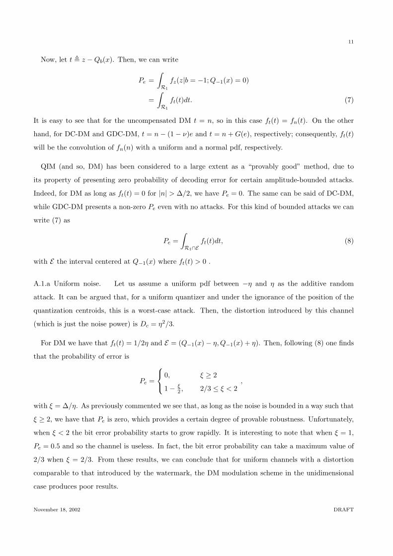
Now, let t , z −Qb(x). Then, we can write

Pe =∫R1

fz(z|b = −1;Q−1(x) = 0)

=∫R1

ft(t)dt. (7)

It is easy to see that for the uncompensated DM t = n, so in this case ft(t) = fn(t). On the other

hand, for DC-DM and GDC-DM, t = n− (1− ν)e and t = n + G(e), respectively; consequently, ft(t)

will be the convolution of fn(n) with a uniform and a normal pdf, respectively.

QIM (and so, DM) has been considered to a large extent as a “provably good” method, due to

its property of presenting zero probability of decoding error for certain amplitude-bounded attacks.

Indeed, for DM as long as ft(t) = 0 for |n| > ∆/2, we have Pe = 0. The same can be said of DC-DM,

while GDC-DM presents a non-zero Pe even with no attacks. For this kind of bounded attacks we can

write (7) as

Pe =∫R1∩E

ft(t)dt, (8)

with E the interval centered at Q−1(x) where ft(t) > 0 .

A.1.a Uniform noise. Let us assume a uniform pdf between −η and η as the additive random

attack. It can be argued that, for a uniform quantizer and under the ignorance of the position of the

quantization centroids, this is a worst-case attack. Then, the distortion introduced by this channel

(which is just the noise power) is Dc = η2/3.

For DM we have that ft(t) = 1/2η and E = (Q−1(x)− η, Q−1(x) + η). Then, following (8) one finds

that the probability of error is

Pe =

0, ξ ≥ 2

1− ξ2 , 2/3 ≤ ξ < 2

,

with ξ = ∆/η. As previously commented we see that, as long as the noise is bounded in a way such that

ξ ≥ 2, we have that Pe is zero, which provides a certain degree of provable robustness. Unfortunately,

when ξ < 2 the bit error probability starts to grow rapidly. It is interesting to note that when ξ = 1,

Pe = 0.5 and so the channel is useless. In fact, the bit error probability can take a maximum value of

2/3 when ξ = 2/3. From these results, we can conclude that for uniform channels with a distortion

comparable to that introduced by the watermark, the DM modulation scheme in the unidimensional

case produces poor results.

November 18, 2002 DRAFT

12

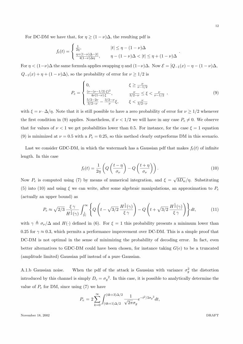
For DC-DM we have that, for η ≥ (1− ν)∆, the resulting pdf is

ft(t) =

12η , |t| ≤ η − (1− ν)∆η+(1−ν)∆−|t|

4(1−ν)∆η , η − (1− ν)∆ < |t| ≤ η + (1− ν)∆.

For η < (1−ν)∆ the same formula applies swapping η and (1−ν)∆. Now E = [Q−1(x)− η − (1− ν)∆,

Q−1(x) + η + (1− ν)∆), so the probability of error for ν ≥ 1/2 is

Pe =

0, ξ ≥ ν

ν−1/2

(ν−(ν−1/2) ξ)2

4ν(1−ν) ξ , ν3/2−ν ≤ ξ < ν

ν−1/2

5/2−2ν3/2−ν − 3/2−ν

ν ξ, ξ < ν3/2−ν

, (9)

with ξ = ν ·∆/η. Note that it is still possible to have a zero probability of error for ν ≥ 1/2 whenever

the first condition in (9) applies. Nonetheless, if ν < 1/2 we will have in any case Pe 6= 0. We observe

that for values of ν < 1 we get probabilities lower than 0.5. For instance, for the case ξ = 1 equation

(9) is minimized at ν = 0.5 with a Pe = 0.25, so this method clearly outperforms DM in this scenario.

Last we consider GDC-DM, in which the watermark has a Gaussian pdf that makes ft(t) of infinite

length. In this case

ft(t) =12η

(Q

(t− η

σν

)−Q

(t + η

σν

)). (10)

Now Pe is computed using (7) by means of numerical integration, and ξ =√

3Dw/η. Substituting

(5) into (10) and using ξ we can write, after some algebraic manipulations, an approximation to Pe

(actually an upper bound) as

Pe ≈√

2/3ξ γ

H12 (γ)

∫ ∞

12γ

{Q

(t−√

3/2H

12 (γ)ξ γ

)−Q

(t +√

3/2H

12 (γ)ξ γ

)}dt, (11)

with γ , σν/∆ and H(·) defined in (6). For ξ = 1 this probability presents a minimum lower than

0.25 for γ ≈ 0.3, which permits a performance improvement over DC-DM. This is a simple proof that

DC-DM is not optimal in the sense of minimizing the probability of decoding error. In fact, even

better alternatives to GDC-DM could have been chosen, for instance taking G(e) to be a truncated

(amplitude limited) Gaussian pdf instead of a pure Gaussian.

A.1.b Gaussian noise. When the pdf of the attack is Gaussian with variance σ2g the distortion

introduced by this channel is simply Dc = σg2. In this case, it is possible to analytically determine the

value of Pe for DM, since using (7) we have

Pe = 2∞∑

k=0

∫ (4k+3)∆/2

(4k+1)∆/2

1√2πσg

e−t2/2σg2dt,

November 18, 2002 DRAFT

13

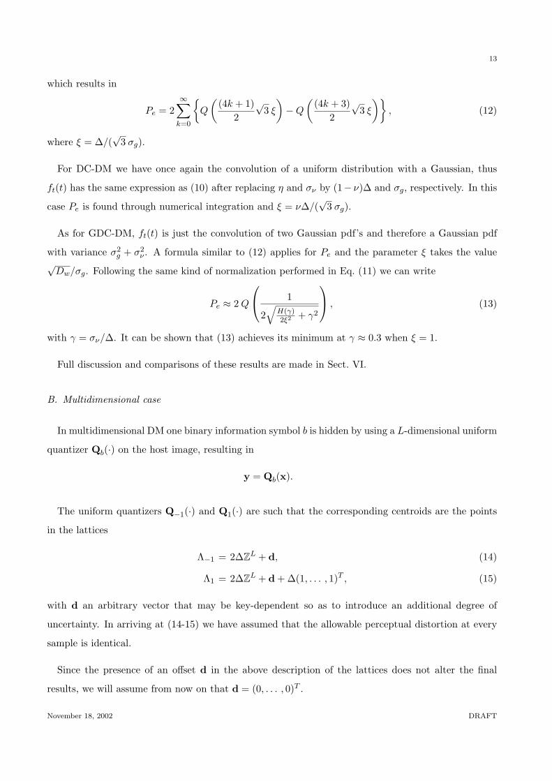
which results in

Pe = 2∞∑

k=0

{Q

((4k + 1)

2

√3 ξ

)−Q

((4k + 3)

2

√3 ξ

)}, (12)

where ξ = ∆/(√

3 σg).

For DC-DM we have once again the convolution of a uniform distribution with a Gaussian, thus

ft(t) has the same expression as (10) after replacing η and σν by (1− ν)∆ and σg, respectively. In this

case Pe is found through numerical integration and ξ = ν∆/(√

3 σg).

As for GDC-DM, ft(t) is just the convolution of two Gaussian pdf’s and therefore a Gaussian pdf

with variance σ2g + σ2

ν . A formula similar to (12) applies for Pe and the parameter ξ takes the value√

Dw/σg. Following the same kind of normalization performed in Eq. (11) we can write

Pe ≈ 2 Q

1

2√

H(γ)2ξ2 + γ2

, (13)

with γ = σν/∆. It can be shown that (13) achieves its minimum at γ ≈ 0.3 when ξ = 1.

Full discussion and comparisons of these results are made in Sect. VI.

B. Multidimensional case

In multidimensional DM one binary information symbol b is hidden by using a L-dimensional uniform

quantizer Qb(·) on the host image, resulting in

y = Qb(x).

The uniform quantizers Q−1(·) and Q1(·) are such that the corresponding centroids are the points

in the lattices

Λ−1 = 2∆ZL + d, (14)

Λ1 = 2∆ZL + d + ∆(1, . . . , 1)T , (15)

with d an arbitrary vector that may be key-dependent so as to introduce an additional degree of

uncertainty. In arriving at (14-15) we have assumed that the allowable perceptual distortion at every

sample is identical.

Since the presence of an offset d in the above description of the lattices does not alter the final

results, we will assume from now on that d = (0, . . . , 0)T .

November 18, 2002 DRAFT

14

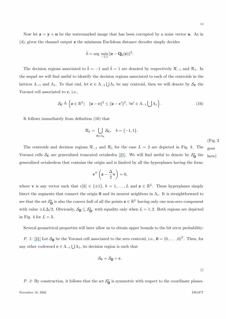
Now let z = y + n be the watermarked image that has been corrupted by a noise vector n. As in

(4), given the channel output z the minimum Euclidean distance decoder simply decides

b = arg min−1,1

‖z−Qb(z)‖2.

The decision regions associated to b = −1 and b = 1 are denoted by respectively R−1 and R1. In

the sequel we will find useful to identify the decision regions associated to each of the centroids in the

lattices Λ−1 and Λ1. To that end, let c ∈ Λ−1⋃

Λ1 be any centroid, then we will denote by Sc the

Voronoi cell associated to c, i.e.,

Sc ,{z ∈ RL| ‖z− c‖2 ≤ ‖z− c′‖2, ∀c′ ∈ Λ−1

⋃Λ1

}. (16)

It follows immediately from definition (16) that

Rb =⋃

c∈Λb

Sc, b = {−1, 1}.

(Fig. 3

goes

here)

The centroids and decision regions R−1 and R1 for the case L = 2 are depicted in Fig. 3. The

Voronoi cells Sc are generalized truncated octahedra [21]. We will find useful to denote by S∗0 the

generalized octahedron that contains the origin and is limited by all the hyperplanes having the form:

vT

(z− ∆

2v)

= 0,

where v is any vector such that v[k] ∈ {±1}, k = 1, . . . , L and z ∈ RL. These hyperplanes simply

bisect the segments that connect the origin 0 and its nearest neighbors in Λ1. It is straightforward to

see that the set S∗0 is also the convex hull of all the points z ∈ RL having only one non-zero component

with value ±L∆/2. Obviously, S0 ⊆ S∗0, with equality only when L = 1, 2. Both regions are depicted

in Fig. 4 for L = 3.

Several geometrical properties will later allow us to obtain upper bounds to the bit error probability:

P. 1: [21] Let S0 be the Voronoi cell associated to the zero centroid, i.e., 0 = (0, . . . , 0)T . Then, for

any other codeword c ∈ Λ−1⋃

Λ1, its decision region is such that

Sc = S0 + c.

2

P. 2: By construction, it follows that the set S∗0 is symmetric with respect to the coordinate planes.

November 18, 2002 DRAFT

15

2

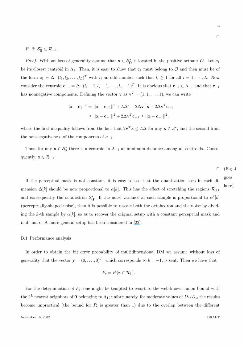
P. 3: S∗0 ⊂ R−1.

Proof. Without loss of generality assume that x ∈ S∗0 is located in the positive orthant O. Let c1

be its closest centroid in Λ1. Then, it is easy to show that c1 must belong to O and then must be of

the form c1 = ∆ · (l1, l2, . . . , lL)T with li an odd number such that li ≥ 1 for all i = 1, . . . , L. Now

consider the centroid c−1 = ∆ · (l1 − 1, l2 − 1, . . . , lL − 1)T . It is obvious that c−1 ∈ Λ−1 and that c−1

has nonnegative components. Defining the vector v as vT = (1, 1, . . . , 1), we can write

||x− c1||2 = ||x− c−1||2 + L∆2 − 2∆vTx + 2∆vTc−1

≥ ||x− c−1||2 + 2∆vTc−1 ≥ ||x− c−1||2,

where the first inequality follows from the fact that 2vTx ≤ L∆ for any x ∈ S∗0 , and the second from

the non-negativeness of the components of c−1.

Thus, for any x ∈ S∗0 there is a centroid in Λ−1 at minimum distance among all centroids. Conse-

quently, x ∈ R−1.

2 (Fig. 4

goes

here)If the perceptual mask is not constant, it is easy to see that the quantization step in each di-

mension ∆[k] should be now proportional to α[k]. This has the effect of stretching the regions R±1

and consequently the octahedron S∗0. If the noise variance at each sample is proportional to α2[k]

(perceptually-shaped noise), then it is possible to rescale both the octahedron and the noise by divid-

ing the k-th sample by α[k], so as to recover the original setup with a constant perceptual mask and

i.i.d. noise. A more general setup has been considered in [22].

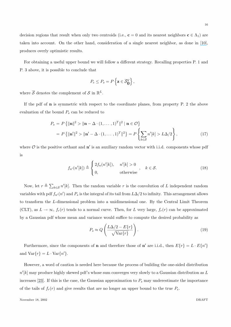
B.1 Performance analysis

In order to obtain the bit error probability of multidimensional DM we assume without loss of

generality that the vector y = (0, . . . , 0)T , which corresponds to b = −1, is sent. Then we have that

Pe = P{z ∈ R1}.

For the determination of Pe, one might be tempted to resort to the well-known union bound with

the 2L nearest neighbors of 0 belonging to Λ1; unfortunately, for moderate values of Dc/Dw the results

become impractical (the bound for Pe is greater than 1) due to the overlap between the different

November 18, 2002 DRAFT

16

decision regions that result when only two centroids (i.e., c = 0 and its nearest neighbors c ∈ Λ1) are

taken into account. On the other hand, consideration of a single nearest neighbor, as done in [10],

produces overly optimistic results.

For obtaining a useful upper bound we will follow a different strategy. Recalling properties P. 1 and

P. 3 above, it is possible to conclude that

Pe ≤ Ps = P{z ∈ S∗0

},

where S denotes the complement of S in RL.

If the pdf of n is symmetric with respect to the coordinate planes, from property P. 2 the above

evaluation of the bound Ps can be reduced to

Ps = P{‖n‖2 > ‖n−∆ · (1, . . . , 1)T ‖2 | n ∈ O

}= P

{‖n′‖2 > ‖n′ −∆ · (1, . . . , 1)T ‖2

}= P

{∑k∈S

n′[k] > L∆/2

}, (17)

where O is the positive orthant and n′ is an auxiliary random vector with i.i.d. components whose pdf

is

fn′(n′[k]) ,

2fn(n′[k]), n′[k] > 0

0, otherwise, k ∈ S. (18)

Now, let r ,∑

k∈S n′[k]. Then the random variable r is the convolution of L independent random

variables with pdf fn′(n′) and Ps is the integral of its tail from L∆/2 to infinity. This arrangement allows

to transform the L-dimensional problem into a unidimensional one. By the Central Limit Theorem

(CLT), as L →∞, fr(r) tends to a normal curve. Then, for L very large, fr(r) can be approximated

by a Gaussian pdf whose mean and variance would suffice to compute the desired probability as

Ps ≈ Q

(L∆/2− E{r}√

Var{r}

). (19)

Furthermore, since the components of n and therefore those of n′ are i.i.d., then E{r} = L · E{n′}

and Var{r} = L ·Var{n′}.

However, a word of caution is needed here because the process of building the one-sided distribution

n′[k] may produce highly skewed pdf’s whose sum converges very slowly to a Gaussian distribution as L

increases [23]. If this is the case, the Gaussian approximation to Ps may underestimate the importance

of the tails of fr(r) and give results that are no longer an upper bound to the true Pe.

November 18, 2002 DRAFT

17

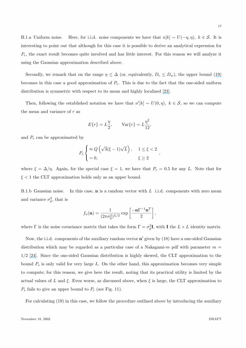
B.1.a Uniform noise. Here, for i.i.d. noise components we have that n[k] ∼ U(−η, η), k ∈ S. It is

interesting to point out that although for this case it is possible to derive an analytical expression for

Pe, the exact result becomes quite involved and has little interest. For this reason we will analyze it

using the Gaussian approximation described above.

Secondly, we remark that on the range η ≤ ∆ (or, equivalently, Dc ≤ Dw), the upper bound (19)

becomes in this case a good approximation of Pe. This is due to the fact that the one-sided uniform

distribution is symmetric with respect to its mean and highly localized [23].

Then, following the established notation we have that n′[k] ∼ U(0, η), k ∈ S, so we can compute

the mean and variance of r as

E{r} = Lη

2, Var{r} = L

η2

12,

and Pe can be approximated by

Pe

≈ Q(√

3(ξ − 1)√

L)

, 1 ≤ ξ < 2

= 0, ξ ≥ 2,

where ξ = ∆/η. Again, for the special case ξ = 1, we have that Pe = 0.5 for any L. Note that for

ξ < 1 the CLT approximation holds only as an upper bound.

B.1.b Gaussian noise. In this case, n is a random vector with L i.i.d. components with zero mean

and variance σ2g , that is

fn(n) =1

(2πσ2g)L/2

exp[−nΓ−1nT

2

],

where Γ is the noise covariance matrix that takes the form Γ = σ2gI, with I the L× L identity matrix.

Now, the i.i.d. components of the auxiliary random vector n′ given by (18) have a one-sided Gaussian

distribution which may be regarded as a particular case of a Nakagami-m pdf with parameter m =

1/2 [24]. Since the one-sided Gaussian distribution is highly skewed, the CLT approximation to the

bound Ps is only valid for very large L. On the other hand, this approximation becomes very simple

to compute; for this reason, we give here the result, noting that its practical utility is limited by the

actual values of L and ξ. Even worse, as discussed above, when ξ is large, the CLT approximation to

Ps fails to give an upper bound to Pe (see Fig. 11).

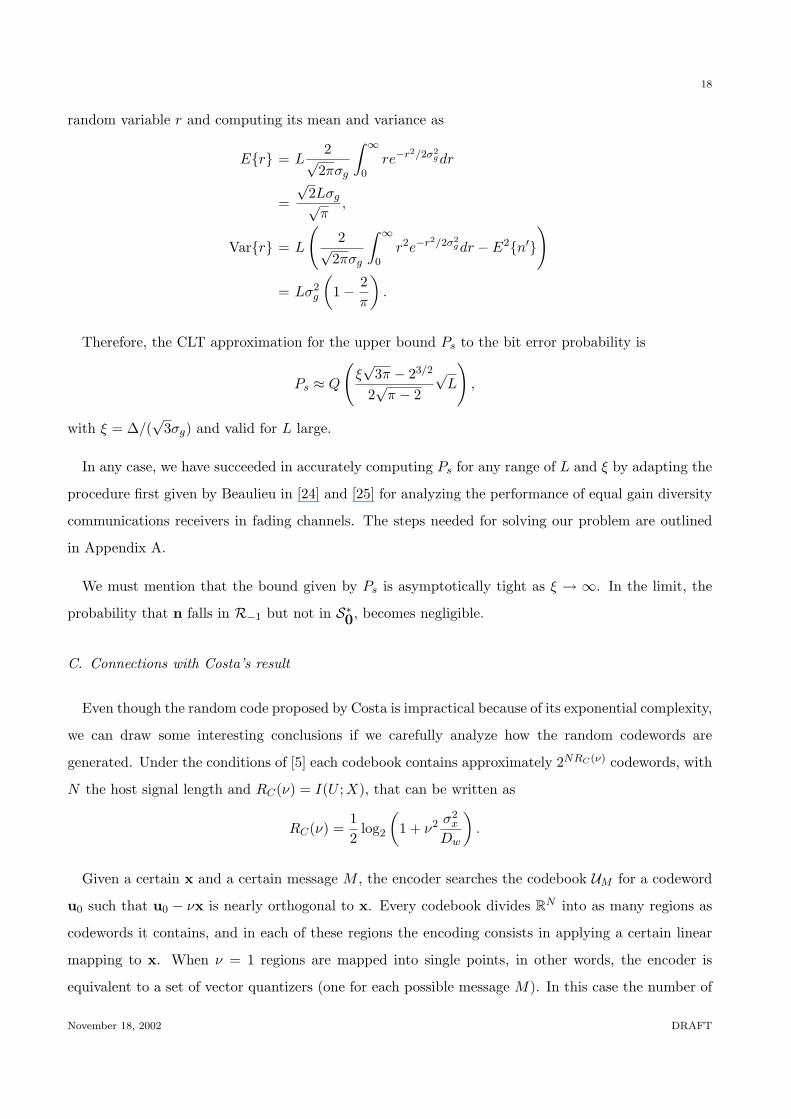
For calculating (19) in this case, we follow the procedure outlined above by introducing the auxiliary

November 18, 2002 DRAFT

18

random variable r and computing its mean and variance as

E{r} = L2√

2πσg

∫ ∞

0re−r2/2σ2

gdr

=√

2Lσg√π

,

Var{r} = L

(2√

2πσg

∫ ∞

0r2e−r2/2σ2

gdr − E2{n′}

)

= Lσ2g

(1− 2

π

).

Therefore, the CLT approximation for the upper bound Ps to the bit error probability is

Ps ≈ Q

(ξ√

3π − 23/2

2√

π − 2

√L

),

with ξ = ∆/(√

3σg) and valid for L large.

In any case, we have succeeded in accurately computing Ps for any range of L and ξ by adapting the

procedure first given by Beaulieu in [24] and [25] for analyzing the performance of equal gain diversity

communications receivers in fading channels. The steps needed for solving our problem are outlined

in Appendix A.

We must mention that the bound given by Ps is asymptotically tight as ξ → ∞. In the limit, the

probability that n falls in R−1 but not in S∗0, becomes negligible.

C. Connections with Costa’s result

Even though the random code proposed by Costa is impractical because of its exponential complexity,

we can draw some interesting conclusions if we carefully analyze how the random codewords are

generated. Under the conditions of [5] each codebook contains approximately 2NRC(ν) codewords, with

N the host signal length and RC(ν) = I(U ;X), that can be written as

RC(ν) =12

log2

(1 + ν2 σ2

x

Dw

).

Given a certain x and a certain message M , the encoder searches the codebook UM for a codeword

u0 such that u0 − νx is nearly orthogonal to x. Every codebook divides RN into as many regions as

codewords it contains, and in each of these regions the encoding consists in applying a certain linear

mapping to x. When ν = 1 regions are mapped into single points, in other words, the encoder is

equivalent to a set of vector quantizers (one for each possible message M). In this case the number of

November 18, 2002 DRAFT

19

codewords per message is 2NRC(1) but, since RC(ν) is increasing with ν, when ν diminishes the number

of codewords per codebook also decreases. In the limit RC(0) = 0 and we have only one codeword;

for this case the encoder is equivalent to an additive watermarking scheme, similar to spread-spectrum

watermarking techniques extensively studied in the literature, in which knowledge of the host signal is

not used by the encoder.

Hence, the value of ν determines how close the encoder is to a pure vector quantizer. When Dc = 0,

a zero probability of error can be achieved with ν = 1, i.e. with a set of quantizers. However, when

Dc 6= 0, it turns out that capacity is not achieved with a set of quantizers, but with a value of ν

less than one. In conclusion, as the noise power Dc increases, it is better to reduce the number of

codewords and let a portion of the host signal pass through the encoder and be superimposed to the

quantization centroid. By doing this, even though part of the host signal appears at the output of the

decoder as what might seem a host interference, the probability of error can be reduced and thus a

higher information rate can be achieved.

IV. Known-host-statistics Methods

These methods rely on a probabilistic characterization of the host data that is employed in order

to develop an optimal (in the Maximum Likelihood, ML, sense) information decoder. This statisti-

cal characterization is available in some domains such as the Discrete Cosine Transform (DCT), the

Discrete Wavelet Transform (DWT) or the Discrete Fourier Transform (DFT). For the sake of simplic-

ity, we will concentrate in the case where x is modeled by a Laplacian pdf, which is adequate when

information is hidden in the DCT domain. Thus, the pdf of each x[k] has the form

fx[k](x) =β[k]2

e−β[k]|x|, (20)

with β[k] =√

2/σx[k]. We allow the Laplacian distribution to vary in each sample of x to better fit

the host signal statistics in the multidimensional case.

One of the most important advantages of these type of methods happens to be the difficulty to

severely modify the host signal’s underlying pdf for a power-constrained channel. This relative invari-

ance of the statistical properties of x is naturally translated into a graceful degradation of performance

in the presence of distortion, as the statistical characterization of the host signal is the basis for the

optimization at the decoding stage. Thus, the Pe yielded at the decoder in a noise-free scenario will not

vary too fast when applying growing channel distortions. Alternatively, disregarding the channel state

introduces an inherent probability of error: those channel uses that are known beforehand to provoke

November 18, 2002 DRAFT

20

an error at the decoder (due to the eventual presence of host signal samples with large amplitudes) are

nonetheless employed for modulating information.

A. Unidimensional case

As in Sect. III we will consider first the unidimensional case. As a representative of the known-host-

statistics family we choose an amplitude modulation method, in which the watermarked sample y is

obtained after adding the watermark w to the host image x. In this case the watermark is computed

from the information symbol as w = sα · b, with s a key-dependent pseudorandom variable for which

E{s2} = 1 and α > 0 a quantity chosen so the perceptual constraint is met. Then, for this method,

Dw = α2.

A.1 Performance analysis

It can be shown [18] that the optimal ML decoder for this scheme decides b = +1 if

|y − sα| < |y + sα|,

or, equivalently, if ys > 0. Let z = y + n the watermarked sample that has been corrupted by additive

noise with pdf fn(n). Assuming that s takes the values ±1 with probability 1/2,1 by symmetry the

bit error probability will be

Pe = P{z > 0 | b = 1} =∫ 0

−∞ft(t− α) dt, (21)

where ft(t) = fn(t) ∗ fx(t). It is interesting to note that in the case when there is no distortion present

in the channel, i.e. n = 0, we have that ft(t) = fx(t) so

Pe =12

e−√

2λ , (22)

with λ = σx/α. Hence, even in the absence of channel distortion, this statistical extraction method

is not “provably robust”: Pe is not zero even for null distortions. Nevertheless, we want to know how

a non-zero distortion would modify this probability by evaluating Pe for the same kind of distortions

presented in Sect. III-A.1.

A.1.a Uniform noise. When n follows a uniform distribution between −η and η, we have that

ft(t) =β

4η

∫ t+η

t−ηe−β|u|du.

1This choice minimizes the bit error probability while meeting the constraint E{s2} = 1. The proof of this fact follows

from the convexity of the integral of the tail of ft(t).

November 18, 2002 DRAFT

21

This integral can be split into two parts yielding

ft(t) =

(1− e−βη cosh(βt)

)/2η, |t| < η

e−β|t| sinh(βη)/2η, |t| ≥ η. (23)

Now, the derivation of Pe becomes simple by using (21):

Pe =

λξ e−√

2/λ

2√

6sinh(

√6

λξ ), ξ >√

312 −

ξ

2√

3+ λξ e−

√6/(λξ)

2√

6sinh(

√2/λ), ξ ≤

√3

,

where now ξ =√

3α/η and λ = σx/α. It is quite important to note that, just as in (22), this probability

of error depends on the DWR (i.e. λ). We can see in Fig. 5 its dependence with this parameter. It

becomes evident that the lower the DWR, the lower the attainable probabilities of decoding error,

reflecting that the statistical knowledge of x is successfully exploited by the decoder. At the same time

the Pe plot becomes less flat when channel distortions are progressively comparable or greater than

Dw because the noise pdf has an increasing relative importance when compared to the pdf of x. (Fig. 5

goes

here)A.1.b Gaussian noise. For the case in which n is a zero-mean Gaussian random variable with variance

σg2 we have that

ft(t) =β

2σg

√2π

∫ ∞

−∞e−β|x|e−(x−t)2/2σg

2dx

=β

2eβ2σg

2/2

{e−βtQ

(−t + βσg

2

σg

)+ eβtQ

(t + βσg

2

σg

)}. (24)

For this distortion, ξ = α/σg, and numerical integration is required for computing Pe after inserting

(24) into (21). As in the previous case, the calculated Pe will be dependent on λ and the previous

discussion on the effects of the DWR applies similarly.

B. Multidimensional case

For the indices selected by S, y is obtained as the addition of the watermark w to the host image

x, where w is computed as w[k] = s[k]α[k] · b, k ∈ S. Note that this choice implicitly uses repetition

coding, allowing for a fair comparison with the results obtained in Sect. III-B. We must recall again

that better encoding alternatives have been explored to enhance these methods [11].

November 18, 2002 DRAFT

22

B.1 Performance analysis

Assuming a Laplacian distribution for x, the ML sufficient statistic [18] can be written as

r ,∑k∈S

β[k]{∣∣y[k] + s[k]α[k]

∣∣− ∣∣y[k]− s[k]α[k]∣∣}.

If without loss of generality we suppose that b = 1 is sent, then r can be written as

r =∑k∈S

β[k]{∣∣x[k] + 2 s[k]α[k]

∣∣− |x[k]|}

=∑k∈S

β[k] P [k]. (25)

Using this statistic, the decision made is b = sgn{r}. For a large value of |S| we may assume a Gaussian

approximation for r, and we compute its mean and variance as

E{r} =∑k∈S

β[k] E{P [k]}

=∑k∈S

(e−2

√2/λ[k] +

2√

2λ[k]

− 1

), (26)

Var{r} =∑k∈S

β2[k] Var{P [k]}

=∑k∈S

(3− e−4

√2/λ[k] − 2 e−2

√2/λ[k]

(1 + 4

√2

λ[k]

)), (27)

with λ[k] = σx[k]/α[k], so Pe depends again on the DWR. When b = −1 the expectation in (26)

just has the opposite sign. The details of the calculation of E{P [k]} and Var{P [k]} can be found in

Appendix B. We have to remark that in the derivation of the first and second order moments of r we

are taking a further step compared to what was done in [18], where the host signal x was considered

to be deterministic.

Thus, we have that the probability of bit error is given by

Pe = Q

(|E{r}|√Var{r}

). (28)

As in Sect. IV-A.1 we get Pe 6= 0 even without considering channel distortions. In the case where

y is corrupted by additive noise n, expressions (26) and (27) have to be recalculated for the pdf of

u = x+n assuming that the optimal detector for the Laplacian case is used regardless of n. In general,

the calculated probabilities will show the observed dependence on the DWR.

Interestingly, for the special case in which λ[k] = λ and the watermark-to-noise ratio is constant

at each sample, a factor√

L appears at the numerator inside Q(·) in (28), thus showing the effect of

repetition coding mentioned in Sect. II.

November 18, 2002 DRAFT

23

B.1.a Uniform noise. In this case n is the uniform noise vector added to the watermarked signal,

with n[k] ∼ U(−η[k], η[k]), k ∈ S. The mean and variance of P [k] are derived in Appendix B.

B.1.b Gaussian noise. When the distortion is Gaussian noise we have again the pdf (24) with partic-

ular parameters for each sample. For this formula closed-form expressions of E{P [k]} and Var{P [k]}

cannot be obtained and we have to resort to numerical integration.

V. Quantized Projection Methods

As it was discussed in the previous section, the performance of known-host-statistics methods be-

comes quite independent of the distortion level that is present in the additive channel. This is at-

tributable to the fact that for high DWR’s the statistics of the host image dominate those of the

additive noise in such a way that the ML detector remains the same despite of channel distortions.

Unfortunately, we will show in Sect. VI how known-host-state schemes usually have better perfor-

mance, especially as the degree of diversity L increases. One can explain this poorer behavior of

known-host-statistics methods by noticing that they are equivalent to using an infinite quantization

step on the decision variable r. Thus, when the host vector x is such that the decision variable r for

the unwatermarked case falls far apart from the decision threshold (here located at the origin), there

is no possibility of effectively conveying an information bit by modifying x so that r falls in the desired

side of the threshold, because of the perceptual limit in the achievable embedding distortion.

This consideration opens the door for other watermarking schemes that effectively combine the

advantages of both known-host-statistics and host-state methods. The idea is to employ a projection

function that produces a scalar decision variable (playing the same role as r in known-host-statistics

methods) but then uniformly quantizing this variable in a similar way as DM methods. For this reason,

we will call the resulting scheme Quantized Projection (QP) method. In implementing this idea, one

faces the problem of finding the watermark such that when added to the host image and later projected,

results in the desired centroid. The fact that r in (25) is nonlinear in the watermark hinders the search

for a solution. As a compromise, we have decided to use a standard cross-correlation for the projection

function, because it is linear and it would be the optimal ML decoding function were the statistics of

the host image Gaussian, as we discussed in [9].

Quantized Projection methods have their roots in the influential proposal by Chen and Wornell of

the Spread-Transform Dither Modulation (STDM) [10], that effectively combines quantization-based

schemes with the diversity afforded by spread-spectrum methods. Specifically, we will stick to the

November 18, 2002 DRAFT

24

particular case of STDM where only one transformed component is quantized since, as we will show,

it yields the minimum probability of error. However, we will depart from this form of STDM to show

that, for large spreading gains, the hypothesis of host data uniform inside the Voronoi cells has to be

abandoned, with the consequence that the size of the cells can be larger and thus the performance can

be better than expected. Unfortunately, as we will see, this perspective complicates the corresponding

theoretical analysis. Another improvement over the original STDM method is that here we will take

into account not only that the embedding power is in general different at each sample, but that this

also occurs to channel distortion (see Section II-A).

Soon after the STDM method was proposed, Ramkumar et al. put forward the idea of improving it by

means of distortion compensation, in what was called Type III schemes [26], computing the achievable

rate for the special case in which the embedding distortion is hard-limited at a certain value. On

the other hand, Eggers et al. considered in [7] the so-called Spread-Transform Scalar Costa Scheme

(STSCS), which is equivalent to compensating the embedding distortion in the STDM method, and

determined its achievable rate. Taking into account that none of these works has dealt with theoretical

error probabilities, in Section V-B we will also give rise to the concept of Distortion-Compensated

Quantized Projection (DC-QP) and analyze its performance.

A. Watermarking with correlation-based uniform quantized projection

In the basic Quantized Projection case, the projection function consists in computing a weighted

cross-correlation between the watermarked image and the watermark, so for a single transmitted bit

the projection r is such that

r ,∑k∈S

y[k]s[k]α[k]

. (29)

In a second stage r is quantized with a uniform scalar quantizer with step 2∆ so the centroids of

the decision cells associated to b = 1 and b = −1 are given by the unidimensional lattices (2-3) with

d = −∆/2, due to symmetry considerations on the pdf of the host signal projection that we will see

next.

It can be shown that dividing by α[k] in (29) becomes the optimal decoding strategy whenever the

noise is perceptually shaped, i.e. when its variance is proportional to the perceptual mask. Although

it is possible to determine the optimal decoding strategy for any other noise joint distribution, this

path will not be taken here. In this regard, it is important to note that the STDM proposal in [10] was

carried out with the same spreading vector for both embedding and decoding stages, which is not our

November 18, 2002 DRAFT

25

case. Of course, the improvement given by the structure proposed in (29) will become important when

the set of perceptual masks α[k], k ∈ S, has a significant ‘spectrum’ and it will be null for constant

perceptual masks.

If w[k] denotes the k-th sample of the watermark, then it is possible to rewrite (29) as

r = rx + rw,

where rw is the projected watermark

rw =∑k∈S

w[k]s[k]α[k]

, (30)

and with a similar definition for the projected host image rx.

The projected watermark rw is selected in such a way that when added to the projected image

rx =∑

k∈S x[k]s[k]/α[k] the result is a member of the desired lattice. Thus, in order to transmit b = 1

the embedder finds rw with the smallest magnitude such that rx + rw ∈ Λ1, which can be immediately

adapted to account for the case b = −1.

Now the problem that faces the embedder is to select the watermark samples w[k], k ∈ S so that

(30) is satisfied. Since there are infinitely many solutions to this problem, it would be possible to

exploit this fact to provide additional robustness against attacks. In fact, this problem resembles

the so-called knapsack problem [27] (an NP-complete one) that was the base for some cryptographic

algorithms although later abandoned for not providing enough security. For our purposes we will

content ourselves with choosing w[k], k ∈ S to become proportional to α[k]. It can be shown that,

under our perceptual constraints, this choice minimizes the probability of error. Then, the watermark

samples are perceptually weighted by their respective masks. Then,

w[k] = ρα[k]s[k], (31)

with ρ a real number that will be determined next. To this end, simply substitute (31) into (30) so

ρ = rw/L and, finally,

w[k] =rwα[k]s[k]

L.

Noticing that rw and the pseudorandom sequence s[k] are statistically independent and that E{s2} = 1,

it is immediate to write

Dw =1L

∑k∈S

E{w2[k]}

=E{r2

w}∑

k∈S α2[k]L3

, (32)

November 18, 2002 DRAFT

26

where L = |S|.

It is interesting to note that while the random variables w[k], k ∈ S are mutually uncorrelated, this

is far from being the case if one considers the random variables w[k] · s[k]/α[k], k ∈ S.

In order to simplify the performance analysis of this data hiding method, let us assume a constant

perceptual mask, i.e., α[k] = α, for all k ∈ S. Although an analysis for varying perceptual masks

is still possible by following the lines here presented, our assumption leads to more compact results.

With this assumption, (32) becomes

Dw =E{r2

w}α2

L2. (33)

Now we are left with the problem of evaluating E{r2w}. To meet this objective, it is necessary to

statistically characterize the random variable rx. Since the s[k], k ∈ S, are statistically independent, it

is possible to resort to the CLT to show that, for large L,2 rx can be accurately modeled by a Gaussian

pdf with zero mean and variance σ2rx

given by

σ2rx

=Lσ2

x

α2, (34)

where σ2x = E{x2[k]}. Of course, a Gaussian pdf also results for any L if the host image x is normally

distributed. In any case, assuming an equiprobable information bit b we have

E{r2w} =

E{r2w|b = 1}+ E{r2

w|b = −1}2

, (35)

where

E{r2w|b = 1} =

∞∑i=−∞

∫ 2(i+1)∆−∆/2

2i∆−∆/2frx(rx)(2i∆ + ∆/2− rx)2drx

=∞∑

i=−∞

∫ 3∆/2

−∆/2frx(rx + 2i∆)(∆/2− rx)2drx

=∞∑

i=−∞

∫ ∆/2

−∆/2frx(rx + 2i∆)(∆/2− rx)2drx

+∞∑

i=−∞

∫ ∆/2

−∆/2frx(rx + (2i + 1)∆)(∆/2 + rx)2drx, (36)

and where frx(rx) is the pdf of rx. Similarly, we can write

E{r2w|b = −1} =

∞∑i=−∞

∫ ∆/2

−∆/2frx(rx + 2i∆)(∆/2 + rx)2drx

+∞∑

i=−∞

∫ ∆/2

−∆/2frx(rx + (2i− 1)∆)(∆/2− rx)2drx. (37)

2The validity of the large L assumption is supported by the results of Sect. V-C.

November 18, 2002 DRAFT

27

Substituting (36) and (37) into (35) and operating, we have

E{r2w} =

∆2

4+

∞∑i=−∞

∫ ∆/2

−∆/2frx(rx + i∆) r2

x drx

= ∆2

(14

+ I(σrx/∆))

, (38)

where

I(σ) ,1√2πσ

∞∑i=−∞

∫ 1/2

−1/2e−(rx+i)2/2σ2

r2x drx. (39)

Having obtained the distortion Dw for arbitrary ∆, σx and α, we will determine the bit error prob-

ability. As before, let z[k] = y[k] + n[k], k ∈ S, where n has zero-mean i.i.d. components with an

arbitrary pdf and variance σ2n, so that Dc = σ2

n. Now the projection r becomes

r = rx + rw + rn,

where the projected watermark rw was defined in (30), and the projected host image rx and noise rn

are similarly defined using x[k] and n[k] respectively instead of w[k].

For large L, we can apply again the CLT to state that for a wide class of distributions in n[k], the

pdf of rn can be approximated by a zero-mean Gaussian pdf with variance σ2rn

equal to

σ2rn

=Lσ2

n

α2=

LDc

α2. (40)

The bit error probability Pe can be determined by taking into account the symmetry in the problem,

so it is enough to consider the errors made when decoding a transmitted b = 1. Similarly to (12), this

probability can be written as

Pe = 2∞∑

k=0

{Q

((4k + 1)∆

2σrn

)−Q

((4k + 3)∆

2σrn

)}. (41)

In order to rewrite Pe in terms of the desired parameters, we may use (33) and (38) to obtain

∆ =√

DwLτ

α, (42)

with τ such that

τ , (1/4 + I(σrx/∆))−1/2 . (43)

Now, using (40) and (42) it is immediate to write

∆σrn

= ξ√

Lτ, (44)

November 18, 2002 DRAFT

28

which can be plugged into (41) to yield the desired expression for Pe. For a further interpretation of

this result, let us write τ in (43) in terms of the DWR, the WNR, and L. Thus, by making use of (42)

and (34), and after some trivial algebra, we obtain

1λ

=√

Dw

σx=

∆√Lσrx

(1/4 + I

(σrx

∆

))1/2

=1√L

F

(∆σrx

), (45)

with the function F (·) defined as

F (x) , x√

1/4 + I(1/x).

It can be shown that F (x) is one to one and monotonically increasing for x > 0. Then, inversion of

(45) yields

∆σrx

= F−1

(√L

λ

), (46)

so, finally, τ can be written as

τ =

1/4 + I

1

F−1(√

Lλ

)−1/2

.

It is easy to see that τ monotonically increases from√

3 to√

4 as the ratio√

L/λ goes from 0 to ∞.

Thus, the parameter τ can be interpreted as a measure of the uniformity of the projected host signal

rx within the quantization bins of size ∆: if frx(rx) is constant within any bin, τ =√

3. However, it is

interesting to see that, as√

L/λ increases, a significant portion of frx(rx) (which will have a Gaussian

shape) will be contained in the two bins closest to the origin and then τ approaches√

4. Consequently,

by increasing L one may obtain an additional gain on the signal to noise ratio of at most 4/3 (1.25

dB), besides the expected diversity gain of L. This additional gain depends not only on L but also on

the document-to-watermark ratio λ, so the smaller the DWR, the larger this extra gain will be if L is

kept constant. From this latter observation we may conclude that Pe actually depends on the DWR as

it happened with known-host-statistics methods, although now in a weaker fashion. Finally, we must

note that, since in practice very large values of L are required for this gain to become significant, this

desirable feature will show up in robust data hiding applications (i.e., for negative WNR’s) where it is

also most welcome.

Last, when ∆/σrn is large, the sum (41) is dominated by the term corresponding to k = 0, so Pe

November 18, 2002 DRAFT

29

can be approximated by

Pe ≈ 2Q

(∆

2σrn

)= 2Q

(ξ√

Lτ

2

),

where again the right-hand side is actually an upper bound to Pe.

B. Distortion Compensated Quantized Projection

The projection function and quantization centroids are the same as in the previous section, as given

by (29) and (2-3). Given the projected host image rx, the projected watermark rw is selected in such

a way that

rw = ν(Qb(rx)− rx), (47)

where Qb(x), b = −1, 1, denotes the closest centroid to x in the lattices Λb, b = −1, 1 given in (2-3),

with d = −∆/2.

The watermark samples are selected according to the method presented in Section V-A, which implies

choosing the scaling factor ρ as in the QP method, where rw is now given by (47). Compared to the

previous method, this Costa-based variant of the Quantized Projection method, which we will term

Distortion Compensated Quantized Projection (DC-QP) in the sequel, scales the quantization error in

the projected domain by ν. This in turn implies that the development in Section V-A for determining

E{r2w} can be easily adapted to the present case to yield

E{r2w} = ν2∆2

(14

+ I(σrx/∆))

, (48)

where I(σ) was given in (39).

Regarding the bit error probability Pe for a zero-mean additive i.i.d. noise channel with distortion

Dc = σ2n, the problem becomes more involved due to the presence of the residual error. We will assume

without loss of generality that the symbol b = 1 is sent. Then, the probability of bit error can be

written as

Pe =∑

i

∫ 2(i+1)∆−∆/2

2i∆−∆/2frx(rx)P (error|rx)drx, (49)

where frx(rx) is the pdf of rx and P (error|rx) is the probability of error for a given value of rx.

Recall that frx(rx) is a zero-mean Gaussian pdf with variance σ2rx

= Lσ2x/α2. In order to determine

P (error|rx), note that if

rx ∈ [2i∗∆−∆/2, 2(i∗ + 1)∆−∆/2), (50)

November 18, 2002 DRAFT

30

for some integer i∗, then following (47) the undistorted projected watermarked image r = rx + rw

becomes

r = νQ1(rx) + (1− ν)rx

= ν(2i∗∆ + ∆/2) + (1− ν)rx.

When ∆/σ2rx

is large, it is possible to simplify the analysis by considering that whenever there exists a

decoding error it is due to rx + rw + rn lying in the Voronoi cells associated to one of the neighboring

centroids to rx + rw in Λ−1, namely, 2(i∗ + 1)∆ −∆/2 and 2i∗∆ −∆/2. From here, it is possible to

conclude that

P (error|rx) ≈ Q

((2i∗ + 1)∆− ν(2i∗∆ + ∆/2)− (1− ν)rx

σrn

)+ Q

(ν(2i∗∆ + ∆/2) + (1− ν)rx − 2i∗∆

σrn

), (51)

where i∗ is such that (50) holds.

After substituting (51) into (49) and after some tedious but straightforward algebraic manipulations

it is possible to arrive at the following result

Pe ≈∑

i

∆√2πσrx

∫ 3/2

−1/2e−∆2(rx+2i)2/2σ2

rx

·[Q

((1 + (1− ν)(1− 2rx))

2νξτ√

L

)+ Q

((1 + (1− ν)(2rx − 1))

2νξτ√

L

)]drx, (52)

where τ was defined in (43). The integral in (52) must be evaluated numerically, but it is interesting

to see that in any case it depends only on ξ, λ, L and ν, i.e. the WNR, the DWR, the number of

dimensions used, and the size of the residual error, respectively. Bear in mind that the ratio ∆2/σ2rx

in (52) may be written as a function of L and the DWR (cf. Eq. (46)). (Fig. 6

goes

here)It is interesting to optimize Pe in (52) in terms of ν. In Fig. 6 we plot Pe as a function of ν for

ξ = 1, L = 20 and for two values of DWR. Some important remarks can be drawn:

• The optimal value of ν that results in each case is smaller than one; hence, note that the DC-QP

method offers to the designer an improvement over the QP method by choosing an appropriate value

of ν. Note that, as QP is equivalent to DC-QP with ν = 1, it is clear that DC-QP for the optimal ν

will never perform worse than QP. However, if the operating WNR is not known at the embedder’s

side (recall that the WNR also depends on the attacking power), it may be safer to set ν = 1, since a

too small ν will increase the bit error probability (cf. Fig. 6).

November 18, 2002 DRAFT

31

• Since the DC-QP scheme resembles Costa’s method, one might expect that the optimal parameter

ν, there derived for maximizing capacity, should become similar to the one here obtained. In Costa’s

paper, the optimal value is ν = 1/(1 + NSR) with NSR the noise-to-signal ratio. In the QP method

the noise to signal ratio after projection becomes σ2rn

/E{r2w} which can be rewritten as

σ2rn

E{r2w}

=Dc

LDw. (53)

Consequently, the NSR for the QP method approaches 0 asymptotically when L → ∞ and then the

optimal value of ν achieved with Costa’s procedure approaches 1 asymptotically for L →∞. Numerical

optimization experiments show that this is in fact the case when Pe is minimized in terms of ν, so that

DC-QP asymptotically approaches QP.

• For moderate L, experimentation shows that the optimal value of ν depends on the ratio Dw/Dc as

is to be expected from (53). Nevertheless, optimization experiments (cf. Fig 6) show that the optimal

ν also depends on the DWR in contrast with Costa’s result in which the host image (there the ‘channel

state’) does not show up in the optimal value of ν. The reason for this difference must be found in the

fact that Costa’s method has unlimited complexity, which is obviously not our case (unless L is made

unpractically large). Interestingly, knowledge of the image second-order statistics becomes useful when

trying to optimize performance. Moreover, for larger DWR’s there is more room for improvement by

choosing the proper value of ν.

C. Generalizing the Distortion Compensated Quantized Projection Method

The DC-QP method described in Sections V-A and V-B can be generalized in such a way that the

quantization operations take place in a vector subspace, introducing dimensionality as an additional

degree of freedom. This idea is borrowed from the general formulation of STDM given by Chen

and Wornell [10] and has the advantage of filling the gamut between the basic DC-QP method and a

multidimensional Distortion Compensated Dither Modulation (DC-DM) method (itself a generalization

of the multidimensional DM scheme), for which the dimensionality of the projected subspace equals

that of the set S. Formally, let M be the dimensionality of the projected subspace, then for the DC-QP

method M = 1, while for the DC-DM method, M = L, with L = |S|.

Then, equation (29) now reads as

r = PTy, (54)

where P = (v1, . . . ,vM ) is a projection matrix with orthogonal columns. Several ways of constructing

November 18, 2002 DRAFT

32

P are possible, all giving essentially the same results, so here we will adopt the simplest, also used

for example in [26], which consists in dividing the set of indices S in M non-overlapping subsets Si,

i = 1, . . . , M , each with cardinality L/M .3 Then, for the i-th vector vi, we have that

vi[k] =

s[k]/α[k] k ∈ Si

0, otherwise.

As before, we can write the projected watermarked image in terms of the projected host image

and the projected watermark, i.e., r = rx + rw. Then, in a generalized QP scheme (that is, with no

distortion compensation), the watermark w should be selected as the minimum Euclidean norm vector

such that r belongs to the desired information-dependent lattice, as in (14-15), with M dimensions

instead of L.

In a generalized DC-QP scheme, w is chosen as the minimum norm vector such that its projection

rw satisfies rw = νe, where ν is a selectable real parameter and e = Qb(rx) − rx, with Qb(·) an

M -dimensional quantizer as in (14-15).

We are interested in determining the value of M that minimizes Pe for a given WNR and for the

optimal value of ν. A similar setup is considered in [26] and [7] to obtain the value of M that maximizes

the achievable rate of a certain data hiding method. In order to keep the discussion simple, we will

assume constant perceptual masks, i.e. α[k] = α, k ∈ S, and i.i.d. Gaussian noise. First, note that the

analysis of Section V-A can be repeated to derive a relation between the projected-noise variance σrn

and the quantization step ∆, so that (44) transforms into

∆σrn

=ξ√

L/Mτ

ν.

Second, the procedure given in Section III-B can be adapted to the present case by considering that

now n[k] should be replaced by the sum of a Gaussian r.v. with variance σrn and a r.v. uniform in

the interval (−(1 − ν)∆, (1 − ν)∆), and noting that, instead of L dimensions, we have M . As for

the DC-DM case, an exact analysis of Pe is not possible, but the method detailed in Appendix A

can also be used to yield an accurate upper bound. Unfortunately, the fact that the pdf of projected

noise is now more involved makes the computations rather lengthy, so they are not included here and

will be published in preliminary form in [22]. With this theoretical upper-bound one can see that the3Here we assume that L/M takes an integer value, neglecting possible border effects. If the M projection vectors are

allowed to overlap, as is done in [10], this problem is completely overcome, even though the analysis turns out to be more

complex. In both cases, the results are equivalent.

November 18, 2002 DRAFT

33

optimal value of M is 1, this meaning that the basic DC-QP gives the best performance in the class

of generalized DC-QP schemes. (Fig. 7

goes

here)To illustrate this, in Figure 7 we depict the probability of error Pe vs. the parameter M for different

WNR’s, showing both the analytical bound (which is asymptotically tight) and the outcome of 8×106

Monte Carlo simulations. For each WNR and M pair, the distortion parameter ν is chosen to minimize

Pe and it is found by exhaustive search. The same tendency (increase in Pe with M) was perceived

for many more WNR’s tested by the authors and not shown here. A further justification for this

behavior is afforded by working with the union bound and making the simplification that the projected-

noise variance follows a Gaussian distribution (as is for instance done in [7]). The advantage of this

formulation is that it allows to analytically obtain the value of ν that minimizes the union bound (and

that happens to be the same as that given by Costa) and then differentiate this bound in terms of

the parameter M . Due to the lack of space, we do not show the calculations here, but note that for

any fixed WNR, the union bound to Pe monotonically increases with M for M > 0.65, which given

the discrete nature of M , provides additional support to the hypothesis that M = 1 produces the

minimum Pe.

Therefore, we conclude that working with just one projected dimension is optimal for this family of

data hiding methods and, as a corollary, that the basic DC-QP method always performs better than

the multidimensional DC-DM scheme. These conclusions are in good agreement with the experimental

results reported by Eggers and Girod in [28], who compared the SCS (equivalently, DC-DM) method

with repetition coding, and the Spread-Transform SCS method, both of which hold close likeness with

our two extremal cases (DC-DM and DC-QP, respectively).

It is also interesting to relate our results to the achievable rates computed in [28] for Spread-

Transform-like methods. As shown there, for Costa’s scheme spreading can only reduce the achievable

rate (the ‘critical slope’ is never attained). The same happens with diversity in digital communications

for Gaussian channels; after all, capacity formulas are identical in both cases. However, this does not

mean that increasing the spreading factor L will ever increase Pe; on the contrary, as readily seen

in (52), L should be made as large as possible, limited only by the payload to be hidden. Of course,

with better coding schemes and/or constellations, it would be possible to fall closer to capacity than

what is achieved through just spreading. Nevertheless, if coding is to be used, spreading may be useful

for pushing up the operating WNR to values for which good codes are known: interestingly, Eggers and

Girod have shown in [28] that for negative WNR’s the Spread-Transform SCS method may increase the

November 18, 2002 DRAFT

34

achievable rate by augmenting L, thus recovering part of the rate that is lost due to the suboptimality

of this data hiding scheme. Since for a given WNR there is an optimal L beyond which the achievable

rate decreases, this suggests concatenating diversity (to improve the WNR) and channel coding.

D. Connections of QP with Costa’s result

We have seen in Sect. III-C that in Costa’s encoding scheme the ν parameter lets a part of the host

signal x traverse the encoder and appear at the input. In fact, when ν = 0 the whole host signal gets

to the output. In the generalized QP, instead of quantizing x we alternatively quantize the projection

of x into a subspace, and leave the part of x orthogonal to that subspace intact.

Let us assume that the projection matrix P given in (54) has M orthonormal columns (note that this

normalization does not have any impact on performance, although ∆ has to be scaled accordingly).

The watermark is computed as

w = P(Qb(P

Tx)−PTx),

where Qb(·) is an M -dimensional quantizer. The watermark can alternatively be expressed as

w = u0 −PPTx,

where u0 = P Qb(PTx) is an L-dimensional codeword, lying in the subspace spanned by {v1, . . . ,vM}.

Therefore, the signal received at the decoder is

z = u0 + (IL −PPT )x + n.

Now, it is easy to see that the role played by ν in Costa’s random coding scheme is now played by

the matrix PPT . The role is similar in the sense that it performs a linear transformation on x with

an energy reduction. The rest of the energy of x, i.e. (IL − PPT )x, or the projection of x onto the

subspace orthogonal to the subspace spanned by {v1, . . . ,vM}, can be employed to compensate for

distortions introduced by the quantizer. Recall that the (1− ν)x term in Costa’s scheme was used in

a similar way.

In fact, for a given maximum average watermark distortion Dw, projecting into a subspace allows us

to increase the size of the quantization cells. As a consequence, the minimum distance between quanti-

zation centroids associated with different messages can be increased. In other words, the performance

against noise can be improved. One may compute the capacity of the QP method assuming that P is

a random matrix, to show that it is lower than that given by Costa.

November 18, 2002 DRAFT

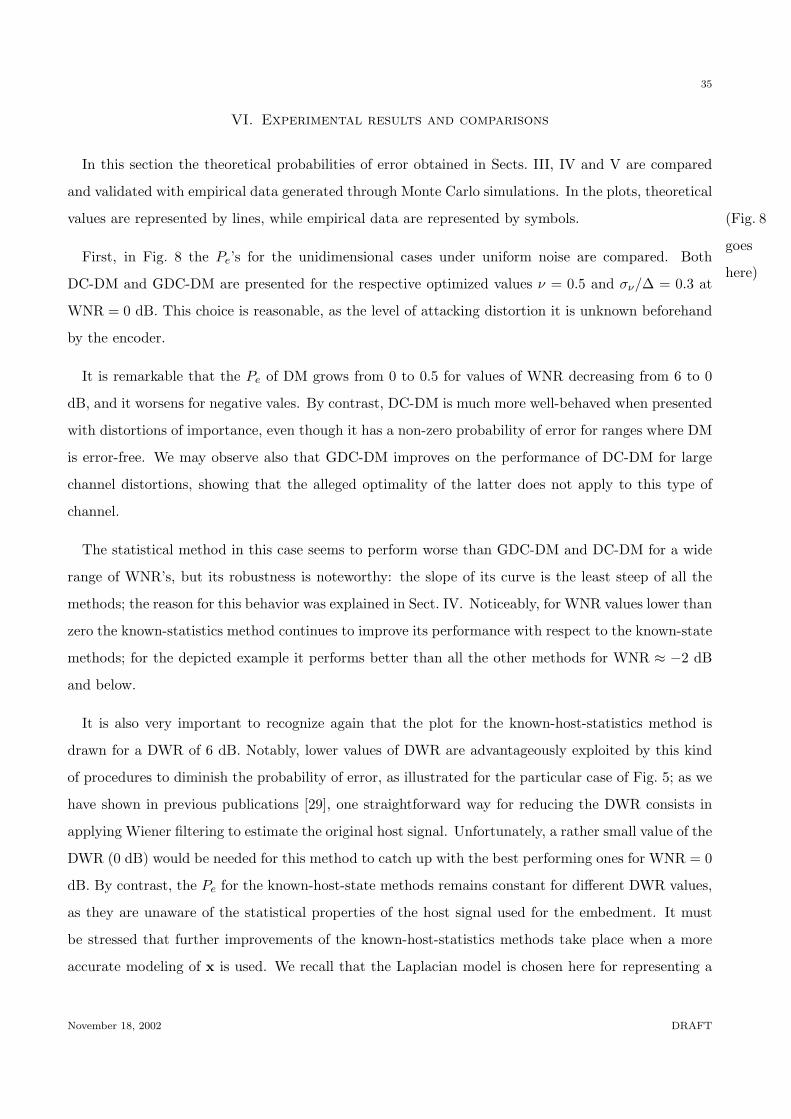
35

VI. Experimental results and comparisons

In this section the theoretical probabilities of error obtained in Sects. III, IV and V are compared

and validated with empirical data generated through Monte Carlo simulations. In the plots, theoretical

values are represented by lines, while empirical data are represented by symbols. (Fig. 8

goes

here)First, in Fig. 8 the Pe’s for the unidimensional cases under uniform noise are compared. Both

DC-DM and GDC-DM are presented for the respective optimized values ν = 0.5 and σν/∆ = 0.3 at

WNR = 0 dB. This choice is reasonable, as the level of attacking distortion it is unknown beforehand

by the encoder.

It is remarkable that the Pe of DM grows from 0 to 0.5 for values of WNR decreasing from 6 to 0

dB, and it worsens for negative vales. By contrast, DC-DM is much more well-behaved when presented

with distortions of importance, even though it has a non-zero probability of error for ranges where DM

is error-free. We may observe also that GDC-DM improves on the performance of DC-DM for large

channel distortions, showing that the alleged optimality of the latter does not apply to this type of

channel.

The statistical method in this case seems to perform worse than GDC-DM and DC-DM for a wide

range of WNR’s, but its robustness is noteworthy: the slope of its curve is the least steep of all the

methods; the reason for this behavior was explained in Sect. IV. Noticeably, for WNR values lower than

zero the known-statistics method continues to improve its performance with respect to the known-state

methods; for the depicted example it performs better than all the other methods for WNR ≈ −2 dB

and below.

It is also very important to recognize again that the plot for the known-host-statistics method is

drawn for a DWR of 6 dB. Notably, lower values of DWR are advantageously exploited by this kind

of procedures to diminish the probability of error, as illustrated for the particular case of Fig. 5; as we

have shown in previous publications [29], one straightforward way for reducing the DWR consists in

applying Wiener filtering to estimate the original host signal. Unfortunately, a rather small value of the

DWR (0 dB) would be needed for this method to catch up with the best performing ones for WNR = 0

dB. By contrast, the Pe for the known-host-state methods remains constant for different DWR values,

as they are unaware of the statistical properties of the host signal used for the embedment. It must

be stressed that further improvements of the known-host-statistics methods take place when a more

accurate modeling of x is used. We recall that the Laplacian model is chosen here for representing a

November 18, 2002 DRAFT

36

good compromise between accuracy and ease of analytical manipulation. More exact models such as

the generalized Gaussian or other heavy-tailed pdf’s have been proposed to model DCT coefficients

with outstanding results [18]. (Fig. 9

goes

here)Fig. 9 shows the performance of the aforementioned methods for the Gaussian case. The Pe vs.

WNR curves corresponding to DC-DM and GDC-DM are depicted for their respective optimum values

ν = 0.53 and σν/∆ = 0.275, at WNR = 0 dB. In general we can draw the same conclusions from

these results as for the uniform noise case although, by comparison with Fig. 8, it becomes clear that

Gaussian noise is not at all a worst case attack for DM, as the largest distortion only causes now a Pe

lower than 0.4. This reveals that analyses of DM under Gaussian channels may overstate its potential.

On the other hand, now the DC-DM method proves to perform better than GDC-DM, thus making

evident that the Gaussian channel fits better to this method. The same reasoning above about the

known-statistics method readily applies here. (Fig. 10

goes

here)Next the multidimensional cases for DM and the known-host-statistics method, under uniform and

Gaussian noise respectively, are presented in Figs. 10 and 11. The performance of the known-host-

statistics method has been evaluated for the particular case of λ[k] = λ and a constant WNR, to allow

for a fair comparison with the known-host-state case that was analyzed under this assumption. The

sensitivity to noise of the latter is evident from a glance at both plots; in addition it becomes apparent,

as in the unidimensional case, that the uniform channel is a worse attack than the Gaussian channel.

Regarding the theoretical approximation used for predicting its performance we can see that, while

the CLT approximation agrees almost perfectly with the empirical results in the uniform case, for the

Gaussian channel it cannot even upperbound the empirical values of Pe when the WNR grows beyond

3 dB. As explained in Sect. III-B this effect is due to the slow convergence of the summation in (17)

to a true Gaussian, considering that we are only using L = 20. Therefore, it is necessary to resort to

the bound derived in Appendix A, that we can see becomes a very tight approximation to Pe for large

values of the WNR.

Last, note that the known-host-statistics method remains now almost invariable for the whole range

of allowed distortions, and, remarkably, for the two different noise sources applied. As in the uni-

dimensional case, the method improves for lower DWR’s by contrast with the invariability of the

known-host-state one. (Fig. 11

goes

here)In Fig. 12 the results for QP and DC-QP are presented. For both cases, the final performance is

excellent, outdoing by several orders of magnitude in Pe the other multidimensional methods with the

November 18, 2002 DRAFT

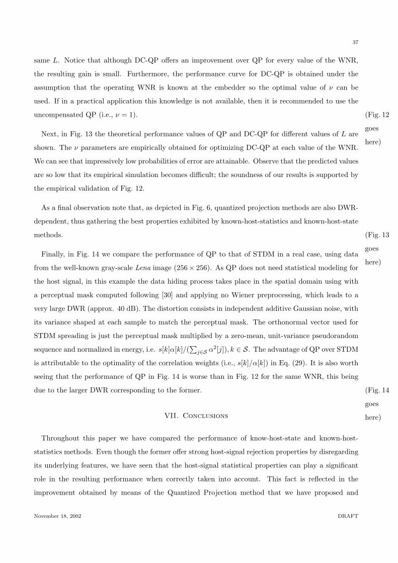
37

same L. Notice that although DC-QP offers an improvement over QP for every value of the WNR,

the resulting gain is small. Furthermore, the performance curve for DC-QP is obtained under the

assumption that the operating WNR is known at the embedder so the optimal value of ν can be

used. If in a practical application this knowledge is not available, then it is recommended to use the

uncompensated QP (i.e., ν = 1). (Fig. 12

goes

here)Next, in Fig. 13 the theoretical performance values of QP and DC-QP for different values of L are

shown. The ν parameters are empirically obtained for optimizing DC-QP at each value of the WNR.

We can see that impressively low probabilities of error are attainable. Observe that the predicted values

are so low that its empirical simulation becomes difficult; the soundness of our results is supported by

the empirical validation of Fig. 12.

As a final observation note that, as depicted in Fig. 6, quantized projection methods are also DWR-

dependent, thus gathering the best properties exhibited by known-host-statistics and known-host-state

methods. (Fig. 13

goes

here)Finally, in Fig. 14 we compare the performance of QP to that of STDM in a real case, using data

from the well-known gray-scale Lena image (256× 256). As QP does not need statistical modeling for

the host signal, in this example the data hiding process takes place in the spatial domain using with

a perceptual mask computed following [30] and applying no Wiener preprocessing, which leads to a

very large DWR (approx. 40 dB). The distortion consists in independent additive Gaussian noise, with

its variance shaped at each sample to match the perceptual mask. The orthonormal vector used for

STDM spreading is just the perceptual mask multiplied by a zero-mean, unit-variance pseudorandom

sequence and normalized in energy, i.e. s[k]α[k]/(∑

j∈S α2[j]), k ∈ S. The advantage of QP over STDM

is attributable to the optimality of the correlation weights (i.e., s[k]/α[k]) in Eq. (29). It is also worth

seeing that the performance of QP in Fig. 14 is worse than in Fig. 12 for the same WNR, this being

due to the larger DWR corresponding to the former. (Fig. 14

goes

here)VII. Conclusions

Throughout this paper we have compared the performance of know-host-state and known-host-

statistics methods. Even though the former offer strong host-signal rejection properties by disregarding

its underlying features, we have seen that the host-signal statistical properties can play a significant

role in the resulting performance when correctly taken into account. This fact is reflected in the

improvement obtained by means of the Quantized Projection method that we have proposed and

November 18, 2002 DRAFT

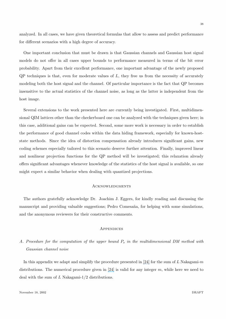
38

analyzed. In all cases, we have given theoretical formulas that allow to assess and predict performance

for different scenarios with a high degree of accuracy.

One important conclusion that must be drawn is that Gaussian channels and Gaussian host signal

models do not offer in all cases upper bounds to performance measured in terms of the bit error

probability. Apart from their excellent performance, one important advantage of the newly proposed

QP techniques is that, even for moderate values of L, they free us from the necessity of accurately

modeling both the host signal and the channel. Of particular importance is the fact that QP becomes

insensitive to the actual statistics of the channel noise, as long as the latter is independent from the

host image.

Several extensions to the work presented here are currently being investigated. First, multidimen-

sional QIM lattices other than the checkerboard one can be analyzed with the techniques given here; in

this case, additional gains can be expected. Second, some more work is necessary in order to establish

the performance of good channel codes within the data hiding framework, especially for known-host-

state methods. Since the idea of distortion compensation already introduces significant gains, new

coding schemes especially tailored to this scenario deserve further attention. Finally, improved linear

and nonlinear projection functions for the QP method will be investigated; this relaxation already

offers significant advantages whenever knowledge of the statistics of the host signal is available, so one

might expect a similar behavior when dealing with quantized projections.

Acknowledgments

The authors gratefully acknowledge Dr. Joachim J. Eggers, for kindly reading and discussing the

manuscript and providing valuable suggestions; Pedro Comesana, for helping with some simulations,

and the anonymous reviewers for their constructive comments.

Appendices

A. Procedure for the computation of the upper bound Ps in the multidimensional DM method with

Gaussian channel noise

In this appendix we adapt and simplify the procedure presented in [24] for the sum of L Nakagami-m

distributions. The numerical procedure given in [24] is valid for any integer m, while here we need to

deal with the sum of L Nakagami-1/2 distributions.

November 18, 2002 DRAFT

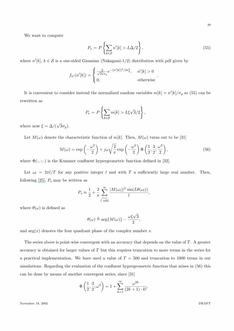
39

We want to compute

Ps = P

{∑k∈S

n′[k] > L∆/2

}, (55)

where n′[k], k ∈ S is a one-sided Gaussian (Nakagami-1/2) distribution with pdf given by

fn′(n′[k]) =

2√

2πσge−(n′[k])2/2σ2

g , n′[k] > 0

0, otherwise.

It is convenient to consider instead the normalized random variables m[k] = n′[k]/σg so (55) can be

rewritten as

Ps = P

{∑k∈S

m[k] > Lξ√

3/2

},

where now ξ = ∆/(√

3σg).

Let M(ω) denote the characteristic function of m[k]. Then, M(ω) turns out to be [31]

M(ω) = exp(−ω2

2

)+ jω

√2π

exp(−ω2

2

)Φ(

12,32;ω2

2

), (56)

where Φ(·, ·; ·) is the Kummer confluent hypergeometric function defined in [32].

Let ωl = 2πl/T for any positive integer l and with T a sufficiently large real number. Then,

following [25], Ps may be written as

Ps ≈12

+2π

∞∑l=1

l odd

|M(ωl)|L sin(Lθ(ωl))l

,

where θ(ω) is defined as

θ(ω) , arg{M(ω)} − ωξ√

32

,

and arg(x) denotes the four quadrant phase of the complex number x.

The series above is point-wise convergent with an accuracy that depends on the value of T . A greater

accuracy is obtained for larger values of T but this requires truncation to more terms in the series for

a practical implementation. We have used a value of T = 500 and truncation to 1000 terms in our

simulations. Regarding the evaluation of the confluent hypergeometric function that arises in (56) this

can be done by means of another convergent series, since [31]

Φ(

12,32;ω2

)= 1 +

∞∑k=1

ω2k

(2k + 1) · k!.

November 18, 2002 DRAFT

40

B. Calculation of E{P [k]} and Var{P [k]} for the known-statistics multidimensional case

We assume that x[k] and s[k] are the only random variables in the expression (25), and that the

latter takes the values ±1 with equal probability. After integrating over s[k] we get the following

expressions for the summands:

E{P [k] |x[k]} =12

(|x[k]|+ 2α[k] +

∣∣|x[k]| − 2α[k]∣∣)− |x[k]|,

Var{P [k] |x[k]} =14

(|x[k]|+ 2α[k]−

∣∣|x[k]| − 2α[k]∣∣)2

.

To ease the manipulation, these equations can be rewritten as

E{P [k] |x[k]} =

−|x[k]|+ 2α[k], |x[k]| ≤ 2α[k]

0, |x[k]| > 2α[k], (57)

Var{P [k] |x[k]} =

x2[k], |x[k]| ≤ 2α[k]

4α2[k], |x[k]| > 2α[k]. (58)

Averaging over the pdf of x[k] we have

E{P [k]} = Ex[k]

{E{P [k] |x[k]}

}, (59)

Var{P [k]} = Ex[k]

{Var{P [k] |x[k]}

}+ Varx[k]

{E{P [k] |x[k]}

}= Ex[k]

{Var{P [k] |x[k]}

}+ Ex[k]

{E2{P [k] |x[k]}

}− E2

x[k]

{E{P [k] |x[k]}

}. (60)

Therefore, for the noiseless case we have to compute the different expectations in (59-60) using the

pdf of x[k] given by (20) and the expressions (57-58), resulting

E{P [k]} =1

β[k](e−2β[k]α[k] + 2β[k]α[k]− 1),

Var{P [k]} =1

β2[k]

(3− e−4β[k]α[k] − 2 e−2β[k]α[k](1 + 4β[k]α[k])

).

For the calculation of the same expectations when uniform noise is added we must use instead the

pdf of t[k] = x[k] + n[k] given by (23). As this pdf is symmetrical and has two parts, for the case

η[k] ≤ 2α[k] we may divide now each integral in the interval [0, 2α[k]) into two integrals in the intervals

[0, η[k]) and [η[k], 2α[k]) respectively. Thus, we can write E{P [k]} as

E{P [k]} = 2∫ η[k]

0(−t + 2α[k]) ft(t | |t| < η[k]) dt + 2

∫ 2α[k]

η[k](−t + 2α[k]) ft(t | |t| ≥ η[k]) dt

=12(4α[k]− η[k]) +

1β2[k]η[k]

(sinh(β[k]η[k]) e−2β[k]α[k] + e−β[k]η[k] − 1

). (61)

November 18, 2002 DRAFT

41

As for Var{P [k]}, using also the same restriction on η[k] we may summarize its calculation in the

following expression

Var{P [k]} = 2∫ η[k]

0t2 ft(t | |t| < η[k]) dt + 2

∫ 2α[k]

η[k]t2 ft(t | |t| ≥ η[k]) dt

+ 2∫ +∞

2α[k]4α2[k] ft(t | |t| ≥ η[k]) dt + 2

∫ η[k]

0(−t + 2α[k])2 ft(t | |t| < η[k]) dt

+ 2∫ 2α[k]

η[k](−t + 2α[k])2 ft(t | |t| ≥ η[k]) dt− E2{P [k]}

=5η2[k]

12+

1β2[k]

(e−β[k]η[k] + 3) +1

β4[k]η2[k]

{e−2α[k]β[k]

(2 sinh(β[k]η[k]) + e−2β[k]η[k] − 1

)− 2 e−β[k]η[k]

(cosh(β[k]η[k])− 1

)− 1

2e−4α[k]β[k]

(cosh(2β[k]η[k])− 1

)}+(η[k]− 8α[k]

β2[k]η[k]− 4

β3[k]η[k]

)e−2α[k]β[k] sinh(β[k]η[k]). (62)

The statistics (61) and (62) can be similarly obtained for the case η[k] > 2 α[k].

References

[1] R. G. van Schyndel, A. Z. Tirkel, and C. F. Osborne, “A digital watermark,” in Proc. IEEE Int. Conference on

Image Processing, (Austin, Texas, USA), pp. 86–89, 1994.

[2] W. Bender, D. Gruhl, N. Morimoto, and A. Lu, “Techniques for data hiding,” IBM Systems Journal, vol. 35, no. 3&4,

pp. 313–336, 1996.

[3] I. J. Cox, J. Kilian, F. T. Leighton, and T. Shamoon, “Secure spread spectrum watermarking for multimedia,” IEEE

Transactions on Image Processing, vol. 6, pp. 1673–1687, December 1997.

[4] I. J. Cox, M. L. Miller, and A. L. McKellips, “Watermarking as communications with side information,” Proceedings

of the IEEE, vol. 87, pp. 1127–1141, July 1999.

[5] M. H. Costa, “Writing on dirty paper,” IEEE Trans. on Information Theory, vol. 29, pp. 439–441, May 1983.

[6] B. Chen and G. W. Wornell, “Preprocessed and postprocessed quantization index modulation methods for digital

watermarking,” in Proc. of SPIE, Security and Watermarking of Multimedia Contents, (San Jose, USA), pp. 48–59,

January 2000.

[7] J. J. Eggers, J. K. Su, and B. Girod, “A blind watermarking scheme based on structured codebooks,” in Proc. of

IEE Conf. on Secure Images and Image Authentication, (London, UK), April 2000.

[8] M. Ramkumar, Data Hiding in Multimedia: Theory and Applications. PhD thesis, New Jersey Institute of Technology,

January 2000.

[9] J. R. Hernandez and F. Perez-Gonzalez, “Statistical analysis of watermarking schemes for copyright protection of

images,” Proceedings of the IEEE, vol. 87, pp. 1142–1166, July 1999. Special Issue on Identification and Protection

of Multimedia Information.

[10] B. Chen and G. W. Wornell, “Quantization index modulation: A class of provably good methods for digital water-

marking and information embedding,” IEEE Trans. on Information Theory, vol. 47, pp. 1423–1443, May 2001.

[11] F. Perez-Gonzalez, J. R. Hernandez, and F. Balado, “Approaching the capacity limit in image watermarking: A

November 18, 2002 DRAFT

42

perspective on coding techniques for data hiding applications,” Signal Processing, Elsevier, vol. 81, pp. 1215–1238,

June 2001. Special Section on Information Theoretic Aspects of Digital Watermarking.

[12] P. Moulin and M. Mıhcak, “A framework for evaluating the data-hiding capacity of image sources,” IEEE Trans. on

Image Processing, vol. 11, pp. 1029–1042, September 2002.

[13] R. B. Wolfgang, C. I. Podilchuk, and E. J. Delp, “Perceptual watermarks for digital images and video,” Proceedings

of the IEEE, vol. 87, pp. 1108–1125, July 1999.

[14] S. Voloshynovskiy, A. Herrigel, N. Baumgartner, and T. Pun, “A stochastic approach to content adaptive digital

image watermarking,” in 3rd International Workshop on Information Hiding, (Desden, Germany), Springer-Verlag,

October 1999.

[15] J. J. Eggers, R. Bauml, and B. Girod, “Digital watermarking facing attacks by amplitude scaling and additive white

noise,” in 4th Intl. ITG Conference on Source and Channel Coding, (Berlin, Germany), January 2002.

[16] P. Moulin and J. O’Sullivan, “Information-theoretic analysis of information hiding.” Preprint, December 2001.

[17] L. Schuchman, “Dither signals and their effect on quantization noise,” IEEE Trans. on Communication Technology

(COM), vol. 12, pp. 162–165, December 1964.

[18] J. R. Hernandez, M. Amado, and F. Perez-Gonzalez, “DCT-domain watermarking techniques for still images: De-

tector performance analysis and a new structure,” IEEE Trans. on Image Processing, vol. 9, pp. 55–68, January

2000. Special Issue on Image and Video Processing for Digital Libraries.

[19] B. Chen and G. W. Wornell, “Provably robust digital watermarking,” in Proc. of SPIE, vol. 3845 of Multimedia

Systems and Applications II, (San Jose, USA), pp. 43–54, 1999.

[20] B. Chen and G. W. Wornell, “Dither modulation: A new approach to digital watermarking and information em-

bedding,” in Proc. of SPIE, vol. 3657 of Security and Watermarking of Multimedia Contents, (San Jose, USA),

pp. 342–353, SPIE, 1999.

[21] J. Conway and N. Sloane, Sphere Packings, Lattices and Groups, vol. 290 of Comprehensive Studies in Mathematics.

Springer, 3rd ed., 1999.

[22] F. Perez-Gonzalez and F. Balado, “Nothing but a kiss: A novel and accurate approach to assessing the perfor-

mance of multidimensional distortion-compensated dither modulation,” in Proc. of the 5th International Workshop

on Information Hiding, Lecture Notes in Computer Science, (Noorwijkerhout, The Netherlands), Springer-Verlag,

October 2002.

[23] K. Bury, Statistical Models in Applied Science. Malabar, Florida: Robert E. Krieger Publishing Company, 1975.

[24] N. C. Beaulieu and A. A. Abu-Dayya, “Analysis of equal gain diversity on Nakagami fading channels,” IEEE Trans.

Commun., vol. 39, pp. 225–234, February 1991.

[25] N. C. Beaulieu, “An infinite series for the computation of the complementary probability distribution function of a

sum of independent random variables and its application to the sum of Rayleigh random variables,” IEEE Trans.

Commun., vol. 38, pp. 1463–1474, September 1990.

[26] M. Ramkumar, A. Akansu, and X. Cai, “Floating signal constellations for multimedia steganography,” in IEEE ICC,

(New Orleans, USA), pp. 249–253, June 2000.

[27] M. R. Schroeder, Number Theory in Science and Communication. Springer Series in Information Sciences, Springer-

Verlag, 2nd ed., 1990.

[28] J. J. Eggers and B. Girod, Informed Watermarking. Kluwer Academic Publishers, 2002.

[29] J. R. Hernandez, F. Perez-Gonzalez, J. M. Rodrıguez, and G. Nieto, “Performance analysis of a 2D-multipulse

November 18, 2002 DRAFT

43

amplitude modulation scheme for data hiding and watermarking of still images,” IEEE J. Select. Areas Commun.,

vol. 16, pp. 510–524, May 1998.

[30] J. R. Hernandez, F. Perez-Gonzalez, and J. M. Rodrıguez, “Coding and synchronization: A boost and a bottleneck for

the development of image watermarking,” in Proc. of the COST #254 Int. Workshop on Intelligent Communications,

(L’Aquila, Italy), pp. 77–82, SSGRR, June 1998.

[31] I. Gradshteyn and I. Ryzhik, Table of Integrals, Series, and Products, 5th Ed. San Diego, USA: Academic Press,

1994.

[32] M. Abramowitz and I. Stegun, Handbook of Mathematical Functions. Washington, USA: National Bureau of Stan-

dards, 1972.

Fernando Perez-Gonzalez (M’90) received a telecommunications engineer degree from the Uni-

versity of Santiago, Spain, in 1990 and the Ph.D. from the University of Vigo in 1993, also in

telecommunications engineering. He joined the faculty of the School of Telecommunications Engi-

neering, University of Vigo, as assistant professor in 1990 and is currently a professor in the same

institution. He has visited the University of New Mexico, Albuquerque, for different periods spanning

ten months. His research interests lie in the areas of digital communications, adaptive algorithms

and digital watermarking. He has been the project manager of a number of projects concerned with digital television and

radio, both for satellite and terrestrial broadcasting. He is coeditor of the book Intelligent Methods in Signal Processing

and Communications (Boston, MA: Birkhauser, 1997), has been Guest Editor of two special sections of the EURASIP

journal Signal Processing devoted to signal processing for communications and has co-edited a Feature Topic of the IEEE

Communications Magazine devoted to digital watermarking. He was the Chairman of the Fifth Baiona Workshop on

Emerging Technologies in Telecommunications, held in Baiona, Spain, in 1999 and will chair the Sixth that will take

place during September, 2003.

Felix Balado received a telecommunications engineering degree from the University of Vigo, Spain,

in 1996. He is currently an associate researcher at the University of Vigo, where he is pursuing his

Ph.D. in the field of watermarking and data hiding.

Juan R. Hernandez (biography unavailable).

November 18, 2002 DRAFT

44

List of Figures

1 Generic data hiding procedure. . . . . . . . . . . . . . . . . . . . . . . . . . . . . . . . . . 45

2 Uniform dithered quantizer. . . . . . . . . . . . . . . . . . . . . . . . . . . . . . . . . . . . 45

3 Centroids and decision regions (L = 2). . . . . . . . . . . . . . . . . . . . . . . . . . . . . . 45

4 Regions S0 and S∗0 (L = 3). . . . . . . . . . . . . . . . . . . . . . . . . . . . . . . . . . . . 46

5 Example of a known-host-statistics method dependence with the DWR (theoretical values). 46

6 Theoretical bit error probability versus ν for different values of the DWR, Dc = Dw and

L = 20. . . . . . . . . . . . . . . . . . . . . . . . . . . . . . . . . . . . . . . . . . . . . . . . 46

7 Performance of generalized QP, using multidimensional DC-DM at the projection (L = 20).

Lines and symbols stand for theoretical values and empirical data, respectively. . . . . . . 47

8 Bit error probability versus WNR for the unidimensional case, uniform noise, DWR = 6.0

dB. Lines and symbols stand for theoretical values and empirical data, respectively. . . . . 47

9 Bit error probability versus WNR for the unidimensional case, Gaussian noise, DWR = 6.0

dB. Lines and symbols stand for theoretical values and empirical data, respectively. . . . . 48

10 Bit error probability versus WNR for the multidimensional case (L = 40), uniform noise.

Lines and symbols stand for theoretical values and empirical data, respectively. . . . . . . 48

11 Bit error probability versus WNR for the multidimensional case (L = 20), Gaussian noise.

Lines and symbols stand for theoretical values and empirical data, respectively. . . . . . . 49

12 Bit error probability versus WNR for Quantized Projection (L = 20), DWR = 25.0 dB.

Lines and symbols stand for theoretical values and empirical data, respectively. . . . . . . 49

13 Theoretical bit error probability versus WNR compared for QP (solid lines) and DC-QP

(dashed lines), for increasing values of L (DWR = 25.0 dB). . . . . . . . . . . . . . . . . . 50

14 Performance comparison between QP and STDM with real data (Lena image) and noise

variance locally proportional to the perceptual mask (L = 20). Lines and symbols stand

for theoretical values and empirical data, respectively. . . . . . . . . . . . . . . . . . . . . . 50

November 18, 2002 DRAFT

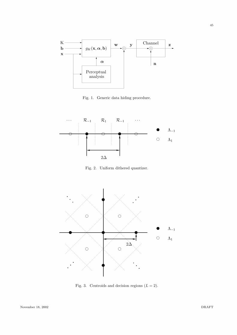
45

PSfrag replacements

x

b

Ky

α

wgK(x,α,b)

Perceptualanalysis

n

zChannel

Fig. 1. Generic data hiding procedure.

PSfrag replacements

2∆

Λ−1

Λ1

R−1R

−1 R1· · · · · ·

Fig. 2. Uniform dithered quantizer.

PSfrag replacements

2∆

Λ−1

Λ1

Fig. 3. Centroids and decision regions (L = 2).

November 18, 2002 DRAFT

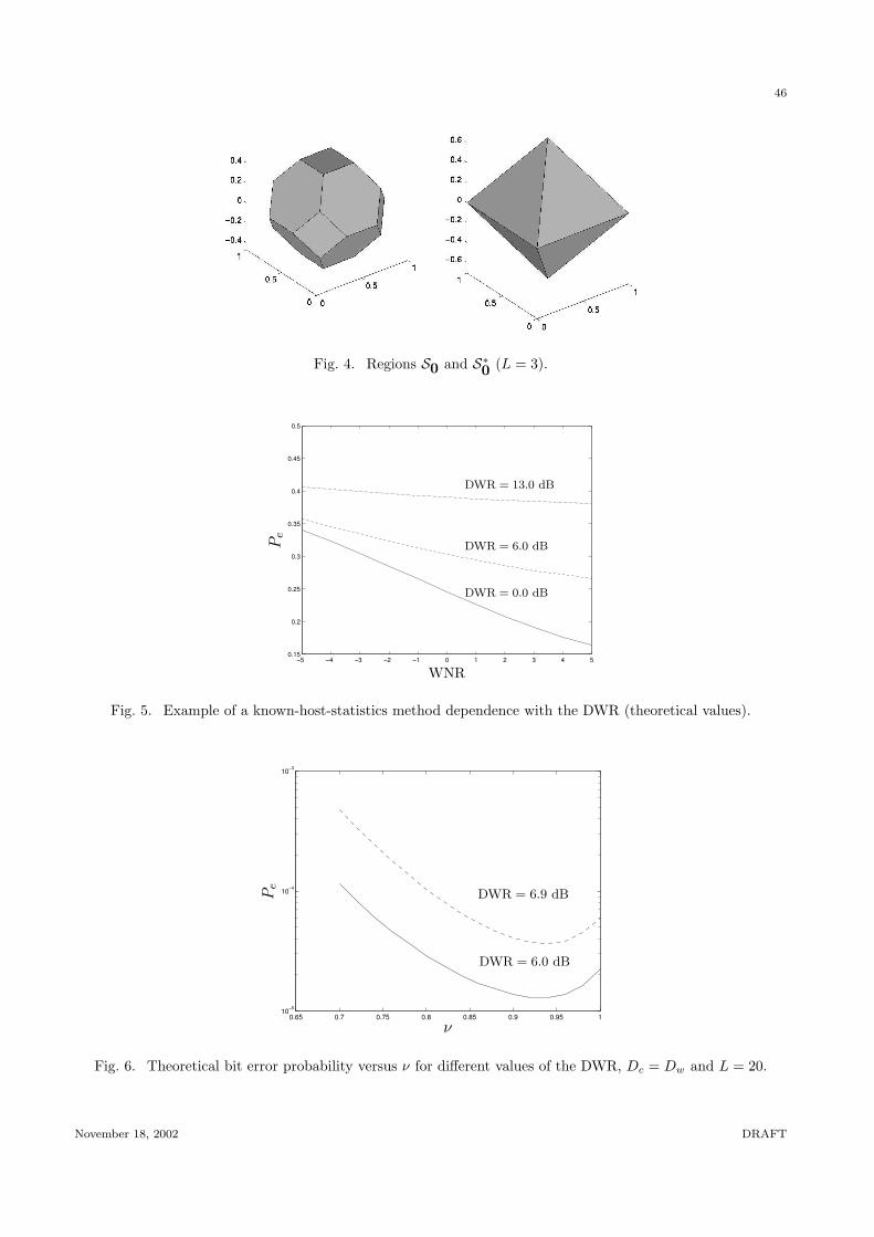
46

Fig. 4. Regions S0 and S∗0 (L = 3).

−5 −4 −3 −2 −1 0 1 2 3 4 50.15

0.2

0.25

0.3

0.35

0.4

0.45

0.5

PSfrag replacements

Pe

WNR

DWR = 13.0 dB

DWR = 6.0 dB

DWR = 0.0 dB

Fig. 5. Example of a known-host-statistics method dependence with the DWR (theoretical values).

0.65 0.7 0.75 0.8 0.85 0.9 0.95 110−5

10−4

10−3

PSfrag replacementsPe

ν

DWR = 6.9 dB

DWR = 6.0 dB

Fig. 6. Theoretical bit error probability versus ν for different values of the DWR, Dc = Dw and L = 20.

November 18, 2002 DRAFT

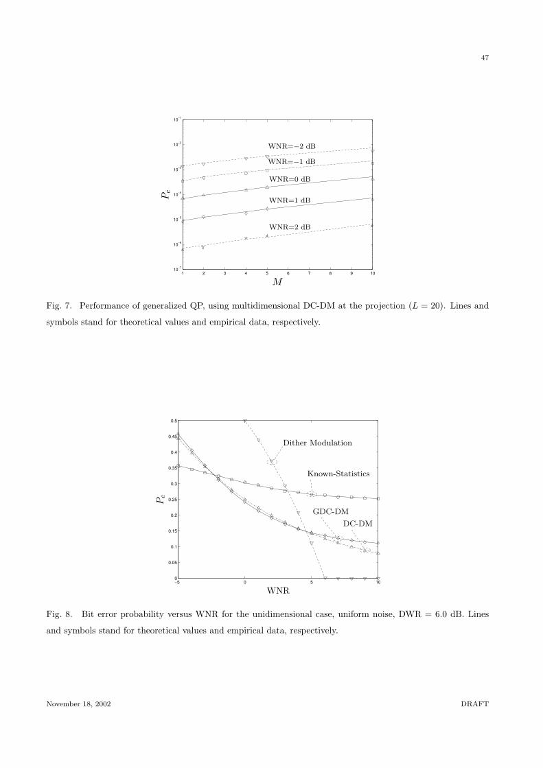
47

1 2 3 4 5 6 7 8 9 1010

−7

10−6

10−5

10−4

10−3

10−2

10−1

PSfrag replacements

Pe

M

WNR=−2 dB

WNR=−1 dB

WNR=0 dB

WNR=1 dB

WNR=2 dB

Fig. 7. Performance of generalized QP, using multidimensional DC-DM at the projection (L = 20). Lines and

symbols stand for theoretical values and empirical data, respectively.

−5 0 5 100

0.05

0.1

0.15

0.2

0.25

0.3

0.35

0.4

0.45

0.5

PSfrag replacements

Pe

WNR

Dither Modulation

DC-DM

GDC-DM

Known-Statistics

Fig. 8. Bit error probability versus WNR for the unidimensional case, uniform noise, DWR = 6.0 dB. Lines

and symbols stand for theoretical values and empirical data, respectively.

November 18, 2002 DRAFT

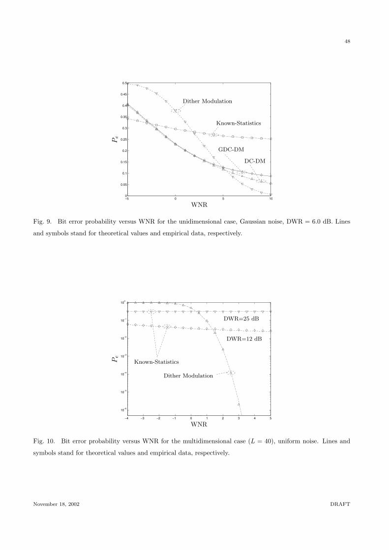
48

−5 0 5 100

0.05

0.1

0.15

0.2

0.25

0.3

0.35

0.4

0.45

0.5

PSfrag replacements

Pe

WNR

Dither Modulation

DC-DM

GDC-DM

Known-Statistics

Fig. 9. Bit error probability versus WNR for the unidimensional case, Gaussian noise, DWR = 6.0 dB. Lines

and symbols stand for theoretical values and empirical data, respectively.

−4 −3 −2 −1 0 1 2 3 4 5

10−6

10−5

10−4

10−3

10−2

10−1

100

PSfrag replacements

Pe

WNR

Dither Modulation

Known-Statistics

DWR=12 dB

DWR=25 dB

Fig. 10. Bit error probability versus WNR for the multidimensional case (L = 40), uniform noise. Lines and

symbols stand for theoretical values and empirical data, respectively.

November 18, 2002 DRAFT

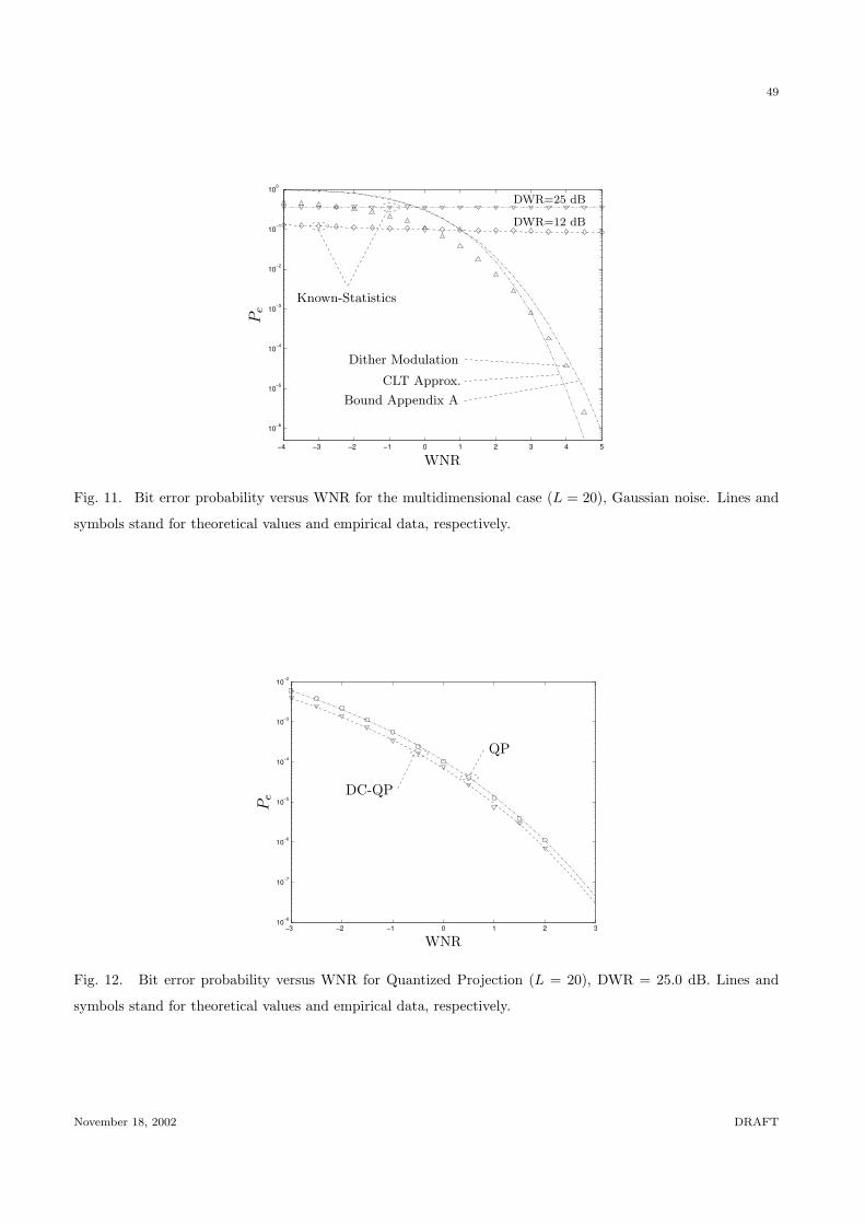
49

−4 −3 −2 −1 0 1 2 3 4 5

10−6

10−5

10−4

10−3

10−2

10−1

100

PSfrag replacements

Pe

WNR

Bound Appendix A

CLT Approx.

Dither Modulation

Known-Statistics

DWR=12 dB

DWR=25 dB

Fig. 11. Bit error probability versus WNR for the multidimensional case (L = 20), Gaussian noise. Lines and

symbols stand for theoretical values and empirical data, respectively.

−3 −2 −1 0 1 2 310

−8

10−7

10−6

10−5

10−4

10−3

10−2

PSfrag replacementsPe

WNR

QP

DC-QP

Fig. 12. Bit error probability versus WNR for Quantized Projection (L = 20), DWR = 25.0 dB. Lines and

symbols stand for theoretical values and empirical data, respectively.

November 18, 2002 DRAFT

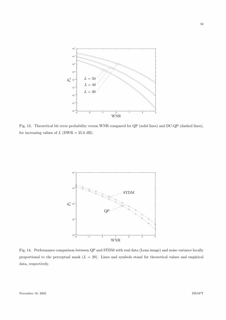
50

−3 −2 −1 0 1 2 310

−18

10−16

10−14

10−12

10−10

10−8

10−6

10−4

10−2

PSfrag replacements

Pe

WNR

L = 30

L = 40

L = 50

Fig. 13. Theoretical bit error probability versus WNR compared for QP (solid lines) and DC-QP (dashed lines),

for increasing values of L (DWR = 25.0 dB).

−2 −1 0 1 2 3 410

−5

10−4

10−3

10−2

10−1

PSfrag replacementsPe

WNR

STDM

QP

Fig. 14. Performance comparison between QP and STDM with real data (Lena image) and noise variance locally

proportional to the perceptual mask (L = 20). Lines and symbols stand for theoretical values and empirical

data, respectively.

November 18, 2002 DRAFT