1

Pattern Discovery for Microsatellite Genome

Analysis

Ioannis Kavakiotisa, Alexandros Triantafyllidisb, Patroklos Samarasa, Antonios

Voulgaridisa, Nikoletta Karaiskoub, Evangelos Konstantinidisb and Ioannis

Vlahavasa

aDepartment of Computer Science, Aristotle University of Thessaloniki, 54124, Greece

bDepartment of Genetics, Development and Molecular Biology, School of Biology,

Aristotle University of Thessaloniki, 54124, Greece

Correspondence: Ioannis Kavakiotis

Email: ikavak@csd.auth.gr

Address: Department of Computer Science, Aristotle University of Thessaloniki, 54124, Greece

Tel: +30-2310-0998145

Fax: +30-231-0998362

Abstract

Microsatellite loci comprise an important part of eukaryotic genomes. Their

applications in biology as genetic markers are related to numerous fields ranging from

paternity analyses to construction of genetic maps and linkage to human disease.

Existing software which offer pattern discovery algorithms for the correct identification

2

and downstream analysis of microsatellites are scarce and are proving to be inefficient

to analyse the large, exponentially increasing, sequenced genomes. Moreover, such

analyses can be very difficult for bioinformatically inexperienced biologists. In this

paper we present MiGA (Microsatellite Genome Analysis) software for the detection of

all microsatellite loci in genomic data through a user friendly interface. The algorithm

searches exhaustively and rapidly for most microsatellites. Contrary to other

applications, MiGA takes into consideration the following three most important aspects:

The efficiency of the algorithm, the usability of the software and the plethora of offered

summary statistics. All the above, help biologists to obtain basic quantitative and

qualitative information regarding the presence of microsatellites in genomic data as well

as downstream processes, such as selection of specific microsatellite loci for primer

design and comparative genome analysis.

Keywords

Bioinformatics Software; Mining methods; Pattern Discovery; Microsatellites; Simple

sequence repeats; Genome Analysis;

1. Introduction

Microsatellites (or simple sequence repeats SSRs) constitute one of the most important

classes of genetic markers, widely applied in an array of research areas, such as studies

of genetic variation and structure, or construction of genetic maps [1]. Some of the most

well known applications in which microsatellites play a key role are paternity testing

[2,3], the confirmation of family pedigrees [4] and forensic investigations [5]. The

3

ubiquity of microsatellites within genomes has played an important role in many genetic

mapping projects such as in human [6], mouse [7], dog [8], trout [9] and other species.

Recently, the advent of next generation sequencing platforms has produced a

wealth of genomic data, permitting a more in depth analysis of microsatellite genome

abundance and distribution across different organisms. In this paper we propose a new

algorithm for the detection of microsatellite loci in genomic data. The algorithm

searches exhaustively for mono-, di-, tri-, tetra-, penta- and hexa- nucleotide

microsatellites and for perfect, imperfect, perfect compound and imperfect compound

microsatellites simultaneously in one execution. The algorithm has been implemented

and is offered in the user friendly application MiGA (Microsatellite Genome Analysis).

The MiGA application, the user manual and example datasets are available on

http://mlkd.csd.auth.gr/bio/miga/index.html

The paper is organized as follows. Section 2 provides some necessary

background knowledge. Section 3 is dedicated to the detailed description of our

approach. This includes the description of the algorithm, the data repository, the front

end and the results. Section 4 presents related work and the existing tools. Section 5

presents results of a task oriented user evaluation. In Section 6, as an example, we

present a full microsatellite analysis of the genome of Danio rerio, (an important

vertebrate model organism). The paper is concluded in section 7.

2. Background Knowledge

4

2.1 Repeated Sequences

The entire genome of an organism contains non-coding regions as well as coding

regions which are translated into proteins. Big parts of non-coding DNA are organized

in repeated sequences. These sequences appear in various sizes and in multiple copies in

the genome and it was initially believed that they had no particular role in biological

processes. Today, it is accepted that they play a significant role in the structure, the

function and the evolution of the genomes and can interact with gene regulatory

mechanisms [11,12,13].

2.1.1 Simple Sequence Repeats - SSRs

Simple Sequence Repeats (SSRs) or short tandem repeats (STRs) constitute a very

common type of repeated sequences (oligomers) in eukaryotic genomes, e.g. (A)n,

(ACAG)n or (GGC)n. The subscript n denotes the number of the repetitions of the

sequence in brackets. This repeated sequence is called motif or pattern. The size of the

motif is 1 to 6 nucleotides long [14]. The number of the repetitions within microsatellite

sequences can vary a lot. whereas their length usually varies from 10 to 300 nucleotides

[14, 15].

2.1.2 The Four Types of SSRs

There are four types of microsatellites. The first type is perfect SSRs constituted by only

one repeat motif e.g. ATGCATGCATGCATGC or (ATGC)4. The only parameter

concerning perfect SSRs is its minimum length. The second type of SSR is imperfect

SSRs which are the same as perfect, but include some mismatch in the repeat sequence,

e.g. (ATGC)3G(ATGC)5. The third type of SSRs is perfect compound SSRs. These are

5

SSRs which constitute of two or more different perfect SSRs e.g. (ACCG)4(GGGC)3.

The last category of SSRs is called imperfect compound SSRs and are constituted from

two or more imperfect SSRs.

3. The MiGA Application

3.1 Pattern Discovery Algorithm for SSR Extraction

MiGA’s algorithm uses an exhaustive search in order to identify microsatellites

in genomes. The algorithm searches for SSRs in a character string (sequence). It finds

the first pattern (1-6 characters) that is repeated and continues by calling itself, with the

remaining substring as input, to identify all the patterns and the number of their repeats.

This was necessary in order to achieve better execution time. This is essential for

complete genome analysis since complete genomes are big datasets and therefore their

analysis with desktop computers is prohibitive.

MiGA‘s algorithm is modular and is divided in two main parts the Repeated

Pattern Discovery and the SSR Assembly.

3.1.1 Repeated Pattern Discovery

The first part of the algorithm is executed only once during the initial loading of

a FASTA file, (the most popular file format in the field of bioinformatics), or during the

initial loading of a full genome from the Ensembl database. Its purpose, in general, is to

extract all perfect repeats (one to six nucleotides long) from the genomic data.

6

Therefore, the algorithm scans the sequence six times (i.e. each time for a different

motif length).

In general, the algorithm places the Beginning Search Position (BSP) at the

beginning of the sequence. The algorithm considers as the first candidate motif the N

long string of nucleotides, which can be found N places after the BSP, BSP included.

For instance, at the first scan, N is equal to one and the candidate pattern is the first

nucleotide of the input sequence i.e the BSP. Considering an input sequence such as:

AGGGCT..., the BSP is nucleotide A, and the candidate mono-nucleotide motif is “A”.

In case of scanning for tri – nucleotide long motifs, the candidate motif would be

“AGG”.

After the identification of the candidate motif, the algorithm checks whether the

N – next nucleotides are the same as the nucleotides of the candidate motif, or simply

put, if the candidate pattern is repeated. If yes, then the algorithm proceeds, until failure

of the comparison and the repeated sequence is subsequently stored in a list along with

its start and finish position. The algorithm will then move the BSP at the first position

after the ending of the repeated sequence.

Consider for example an input sequence to be the following: AAAGTTCT…CTC.

In the first scan of the sequence, for mononucleotide SSRs, the BSP is at the first

nucleotide and the candidate pattern is “A”. The algorithm will check and find this

pattern two additional times. After this, the comparison fails, the algorithm saves the

pattern “A” in a list, along with the starting and ending position and moves the BSP to

7

nucleotide G, right after the repeated sequence “AAA”. The candidate sequence is now

“G”. In case of tri – nucleotide long motifs, the first candidate motif would be AAA.

This motif is clearly not repeated, so the BSP would move on to the second A and the

pattern “AAG” would become the candidate motif.

Completion of the perfect repeated sequence search is followed by a number of

modifications and filtering of results. The most important, is that, to avoid redundancy,

the algorithm assigns a repeated sequence as a sequence with the minimum length of

motif with the most repetitions. For instance, for a repeated sequence

AAAAAAAAAAAA, the algorithm has initially stored this as repetition of motif “A”

twelve times, repetition of motif “AA” six times, etc. After filtering, the algorithm

stores this only as a twelve times repeated motif “A”.

3.1.2 SSR Assembly

The second part of the algorithm, depends heavily on the first and is executed

only according to a specific search requested from the user. Unlike the first part, it is

executed every time there is a new search request, with different parameters. There are

four main functions for this part, related to the four microsatellite types (perfect,

imperfect, perfect compound and imperfect compound SSRs).

The simplest function is the one concerning perfect SSRs. In order to find the

perfect SSRs, the algorithm simply subtracts the end position of a putative SSR from its

start position (as available from the first part of the algorithm). The size of a perfect

SSR should be greater than the minimum length value, supplied by the user as a

8

parameter. For instance, if the minimum SSR length was set to 16, then the sequence

(ATGC)3 would not be considered as a microsatellite. A second function produces

sequences assigned to imperfect SSRs. After finding all perfect SSRs the algorithm

checks if the distance between consecutive perfect SSRs is even or shorter than the

maximum allowed mismatch that has been provided by the user. Our definition of an

imperfect microsatellite does not take into consideration the nature of the mutations of

the possible mismatch and how they resemble or not the correlated repeat motif. To be

assigned as an imperfect SSR, the algorithm also checks if the two patterns of the

perfect SSRs belong to the same repeating cycle. Consider the following imperfect SSR:

“ATGATGCTGATGA”. The algorithm accepts this SSR as an imperfect one, because

the pattern TGA and the pattern ATG belong to the same repeating cycle (i.e. patterns

ATG, GAT and TGA are equivalent).

The third function assembles perfect compound SSRs. It operates in the same

way as with imperfect SSR search, with only small changes to the conditions of

acceptance. Firstly, two consecutive SSR sequences should not be equivalent, unlike

imperfect SSRs which should belong to the same repeating cycle. Secondly, these two

consecutive perfect SSRs should have an (intergenic) distance even or shorter than the

one provided by the user and lastly, the length of every individual repeated pattern

should be even or greater than the minimum length provided by the user.

The last function, concerning imperfect compound microsatellites operates in the

same way as the third function with one difference. At least two of the consecutive

9

repeated sequences must belong to the same repeating cycle, though another repeated

consecutive sequence should exist with a different motif.

3.1.3 General Comment for the Algorithm

We would like to mention the importance of the algorithm’s modular nature. In

general, when performing an analysis of a dataset, biologists tend to analyze the same

datasets many times with different parameters. Having realized this, we constructed the

algorithm in this modular way in order to avoid the repetition of pattern discovery

(section 3.1.1) which is the most time consuming. When there is a new request to

analyze the same data with different parameters, only the second part (SSR Assembly

3.1.2) will be executed.

3.2 Data Repository

Taking into consideration the size of the data and the information that can be

downloaded and analyzed when using the Ensembl database through the program, it

became clear that a local Data Repository (DR) should be used in order to store all

Ensembl originated data. This data can be used in downstream (as well as future)

analyses of MiGA. The DR consists of two parts, a database and a collection of files.

The first part called LoBiD (LOcal BIology Database), is designed and organized in the

same way as commercial databases (Figure 1). LoBiD consists of five tables which refer

to the organism, slices (which are fragments of the DNA sequence), genes, transcripts

and exons. The table organism contains the scientific name of the organism, the id of

the organism in the Ensembl database, the information whether this organism has an

organized karyotype in the Ensembl database or not and the names of the chromosomes

10

in case of karyotype existence. Lastly, this table contains the information about the last

update of the particular organism in LoBiD. The remaining four tables contain

information about the DNA sequences of this organism.

The second part of the DR consists of files which contain the sequences and the

results from the performed analysis. The use of files for storing the DNA sequences was

essential, for the efficient and rapid process of the data. The two parts of the database

are closely related. In other words, the files contain the raw data of the genome and the

database contains all the information about the structure of the genome (i.e. location of

genes, names of chromosomes). The existence of the data repository also allows the

user to restore the search history and retrieve previous projects and consequently, to

perform analysis on previously seen data in a very fast way. The term history has a

twofold meaning. Firstly, the application stores the Repeated Pattern Algorithm analysis

(for each FASTA file or genome) in binary files in the DR. Therefore, in future SSR

discovery analyses, this part of the algorithm does not run again, saving time. Secondly,

the application stores the specific analysis parameters, in order to avoid re-execution of

the algorithm in case the requested analysis is done on the same data with identical

parameters.

3.3 Functionality Overview and Front – End Description

11

3.3.1 Source of Data

MiGA gives the user the opportunity to choose the source of the data that will be

analyzed. MiGA’s first window has two tabs which correspond to the two different

possible ways for providing data to the application. The first way is to search for

microsatellites within user provided data in FASTA format. One single file can contain

multiple sequences. Users should specify a name for the project. MiGA will store all

results in a folder with the project’s name in the data repository. In this step, MiGA also

allows the user to retrieve all previous projects in a dropdown menu, in case the user

would like to analyze previous data.

The second option is the analysis of complete genomes. The complete genome

analysis is made though the Ensembl database [10], the most comprehensive database

for fully annotated eukaryotic genomes. The user can choose from available Ensembl

organisms and then MiGA downloads the selected genomes in the DR.

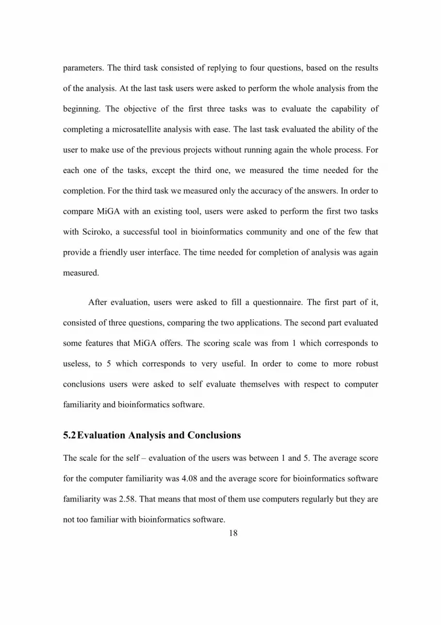
3.3.2 Parameters for SSR Discovery

MiGA allows the user to search for mono-, di-, tri-, tetra-, penta- and hexa- nucleotide

SSRs and for perfect, imperfect, perfect compound and imperfect compound SSRs

simultaneously in one execution (Figure 2). The user should specify the appropriate

parameters for each type of SSR. In case of perfect SSRs the parameter is only the

minimum SSR length, in base pairs. In case of imperfect SSRs the user should provide

i) the maximum length of the gap/mismatch and ii) the minimum length of each SSR.

For compound SSRs the parameters are i) the minimum length of the SSRs and ii) the

12

maximum inter-repeat region (i.e. the region between the two perfect SSRs) that will be

allowed.

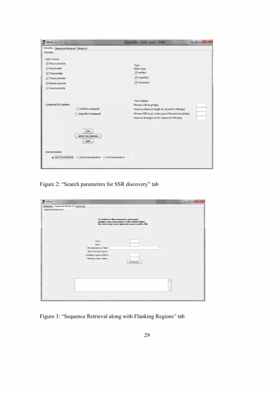
3.3.3 Sequence Retrieval and Flanking Regions

One important aspect when analyzing microsatellite sequences, is to clarify the

composition of the flanking regions of each microsatellite locus. The retrieval of those

regions is important for primer design for downstream analyses of microsatellite loci, or

for comparisons of different loci in different species. There is therefore a tab for

sequence retrieval (Figure 3)

In order to retrieve one SSR sequence, the user has to copy the path, which is the

subdirectory from the root folder to the file that contains the SSR, the start and the end

of the SSR as given in the results file. The program identifies the SSR and the slice

from which it is retrieved in the local database (LoBiD) and provides the user interface

with the sequence as it is. In the same way, the program provides the user the additional

opportunity of flanking regions retrieval for each SSR. The user should specify the

length of the upstream and downstream flanking region.

3.4 Results and Statistics

At the end of the data analysis, the application produces results and summary qualitative

and quantitative statistics, saved in text files. Those files are stored in a local folder with

a folder for every different project in the data repository.

13

3.4.1 Results

Each result file starts with a header which contains the project’s name and all the search

parameters used. Then, follows information about SSRs found during the analysis. This

analytical information includes the motif of the SSR found, the number of repeats for

each SSR, the start and end position in the sequence and lastly the path from where the

user can retrieve the SSR sequence and its flanking regions.

3.4.2 Summary Statistics

The application produces a text file, called motifStatistics, which contains analytical

information for each exact motif found in the sequences, based on the Repeated Pattern

Discovery algorithm (3.1.1). This information includes how many times the motif is

found in the genome (count), the total number of the repeats of the motif (repeats), the

count of the nucleotides in base pairs (bp) which is the product of the length of the motif

multiplied with the repeats, the average microsatellite length (Avg_Length), the

standard deviation of the average microsatellite length (SD_Length), the maximum

length (Max_Length) and the average motif repeat (Avg_Repeats). Moreover, the

application provides the percentage of each nucleotide in a microsatellite motif.

The user can specify whether the program produces standardized, partially

standardized or non standardized results. The standardization, partial or not, is a process

in which similar, microsatellite motifs are grouped together. More precisely, partial

standardization considers as equivalent motifs that belong to the same repeating cycle.

Full standardization takes into account the reverse complements of microsatellite motifs

as well, based on the notion that sequencing machines produce DNA sequences of both

14

strands and therefore of unknown direction. The matrices for the standardization process

are the same with the Sciroko tool [16].

MIGA also produces a summary table for each SSR type (i.e. perfect, imperfect,

perfect compound, imperfect compound). The statistics offered by the application are

the following: The count of each type of SSR, the total size of each type of SSR, the

percentage of each nucleotide (A, G, T, C) found in SSRs, the relative frequency of

each type of SSR (i.e. count of SSRs / total count of SSRs), abundance (i.e. total size of

each type of SSR/ total genome length) and relative abundance (i.e. total size of each

type of SSR/ total length of SSR found in the genome). The text file that contains the

statistics is also generated in html format for more usability.

4. Related Work

Microsatellites present wide applications in the field of biology. Thus their

analysis is a research area with many branches, especially now that genome information

is increasingly available. For instance, LobSTR [17] and RepeatSeq [18] are such new

applications that aim to infer diploid genotypes in microsatellite loci after full genome

sequencing of individuals based on pre-existing reference genomes. Another new

branch in microsatellite analysis is to trace microsatellite loci within assembled or non-

assembled genomes of any kind of species (non-model included). MiGA belongs to this

category.

Several tools already exist in this category based on different approaches and

methodologies [19]. Some of the most important tools are TROLL [21], STAR [22],

15

MISA [23], SSRFinder [24], SSRIT [25], TRF [20], Sciroko [16], QDD [26], Sputnik,

Modified Sputnik I [27] and Modified Sputnik II [28]. Some tools use a dictionary

approach which means that the motifs have to be defined in the program, while others

use heuristic approaches. The first algorithms developed to address the problem of

finding SSRs in genomes used exhaustive search. In the past, these algorithms were

condemned to be applied only in small sequences due to lack of processing power of

computers. Nowadays, that this problem has been solved, many new tools [29, 30]

prefer this methodology in order to be more precise than the heuristic ones. Regardless

of the methodology, the purpose of these tools has to be the identification of repeats in a

DNA sequence, without a priori knowledge of the repeat unit’s composition [20].

Moreover, there should be no limitations in the motif, motif length, and the number of

copies that can be detected [19].

In many publications of previously developed programs such as TROLL, STAR

and others, comparisons were made using as main criteria only the number of hits and

the overall execution time, simplistically concluding that the less execution time and the

more hits, the better the tool. In 2009 Jentzsch published her PhD dissertation [19]

providing a detailed presentation and comparison of the most important existing tools.

One of the key conclusions was that the input parameters should be fine – tuned

individually for each program, so that searches can become equivalent; i.e. there is no

meaning in comparing different tools, if these tools are not looking for the same thing.

This process requires deep knowledge of the various existing programs. An additional

16

main characteristic that Jentzsch considers in her study was the capability of the

program to analyze large sequences in the order of millions of nucleotides.

Although, as just stated, a thorough comparison with an existing tool is a

difficult process, in this section we are going to provide a qualitative comparison

between MiGA and TRF [20] which is the most widely used tool in microsatellite

analysis. The first and main difference is that TRF is a heuristic approach which

performs approximate search in sequences. On the contrary, MiGA performs an

exhaustive search which means that it will discover every microsatellite in a given

sequence with respect to the aforementioned definitions. Another difference is that

MiGA offers the possibility to run a complete search of perfect, imperfect and

compound perfect together or distinctively. TRF does not offer this option. For instance,

due to the probabilistic nature of the algorithm TRF cannot search exclusively for

perfect repeats. Another difference is that TRF produces some redundant hits. MiGA

filters them and presents only SSRs with the minimum motif, as explained earlier.

Moreover, MiGA also offers motif standardization, summary statistics, connection to

online database and history options, all utilities that TRF does not offer.

Overall, available tools lack some or all of the following characteristics: i) a

graphic user-friendly interface ii) summary SSR statistics, iii) connection to an online

database, iv) use of a local database to store and retrieve results and data, v) full genome

SSR search efficiently and fast, and vi) complete search in one execution. MiGA offers

all these characteristics in a very easy way to accomplish.

17

5. User Evaluation

Biologists could be a very diverse group concerning being conversant with computers.

A bioinformatics application can be judged inside the scientific community, in terms of

success, based on the simplicity and the ease of accomplishing tasks. It is common

sense that one of the most important aspects in software design is the usability.

Usability can be measured in various ways, but one of the most reliable is through a task

oriented evaluation, which is performed by ordinary users who had no involvement in

the process of designing and developing the application. Inside knowledge of the whole

project, makes designers and developers unsuitable for identification of possible flaws

in the design and more generally, for performing an unbiased evaluation of a software‘s

usability. For all the reasons presented above, we conducted a task oriented user

evaluation. The purpose of this evaluation was to identify possible flaws and drawbacks

in the design and to measure the application‘s usability.

5.1 Evaluation Description

Our user evaluation involved 12 users, mostly postgraduate students from the

Biology Department of the Aristotle University of Thessaloniki, as well as research staff

from our lab (9 biologists and 3 computer scientists). It is important to mention that no

user was familiar with the application. The evaluation was designed in a way that

simulates a complete microsatellite analysis by a biologist. It consisted of four tasks

which were strongly dependent as consecutive parts of the analysis. At the first task

users were asked to start the application, load the data for analysis and give a specific

project name. The second task was the analysis of the data with some specific

18

parameters. The third task consisted of replying to four questions, based on the results

of the analysis. At the last task users were asked to perform the whole analysis from the

beginning. The objective of the first three tasks was to evaluate the capability of

completing a microsatellite analysis with ease. The last task evaluated the ability of the

user to make use of the previous projects without running again the whole process. For

each one of the tasks, except the third one, we measured the time needed for the

completion. For the third task we measured only the accuracy of the answers. In order to

compare MiGA with an existing tool, users were asked to perform the first two tasks

with Sciroko, a successful tool in bioinformatics community and one of the few that

provide a friendly user interface. The time needed for completion of analysis was again

measured.

After evaluation, users were asked to fill a questionnaire. The first part of it,

consisted of three questions, comparing the two applications. The second part evaluated

some features that MiGA offers. The scoring scale was from 1 which corresponds to

useless, to 5 which corresponds to very useful. In order to come to more robust

conclusions users were asked to self evaluate themselves with respect to computer

familiarity and bioinformatics software.

5.2 Evaluation Analysis and Conclusions

The scale for the self – evaluation of the users was between 1 and 5. The average score

for the computer familiarity was 4.08 and the average score for bioinformatics software

familiarity was 2.58. That means that most of them use computers regularly but they are

not too familiar with bioinformatics software.

19

In order to compare MiGA’s and Sciroko’s user interface, a repeated measures

T-test was conducted to compare the time needed for the completion of the first two

tasks in both applications. T – test assumes that the data follow normal distribution. In

order to test the normality of the data, we conducted a Shapiro – Wilk test which is

appropriate for small sample sizes (<50 samples). The significance values for the

Shapiro – Wilk test are 0.378 and 0.639 for MiGA and Sciroko respectively, proving

that data follow normal distribution. Results of the repeated measures T-test show that

there was a significant difference in the scores for MiGA (M= 97.33, SD= 29.199) and

Sciroko (M= 201.58 , SD= 48.801) conditions; t(11)= -7.225, p=0.000. Although these

results are based on a limited sample of twelve individuals, they suggest that MiGA

does have a more friendly and intuitive user interface.

This result was also confirmed by the questionnaire. All users responded that

they found MiGA to be more user friendly. Admittedly the users were familiar with the

developing team so the questionnaire comparison might be biased.

Lastly, the analysis of the questionnaire concerning the features offered by

MiGA showed that the following were the most important for the users: Project history,

analysis of whole genomes from Ensembl, the short execution time and the html

presentation of the results which offers better visualization of the results.

6 Results of Full Genome analysis of Danio rerio

Zebrafish (D. rerio) is a tropical freshwater fish and a model organism for the science of

biology [31, 33, 34]. Its sequencing project started in 2001 by the Sanger Institute and

20

from then on several assemblies have been released. Its full genome was published in

2013 [32]. The assembly of Zebrafish’s genome that has been analyzed was

1.357.051.643 base pairs (bp). The parameters used for the microsatellite analyses, for

each type were: i) Perfect SSRs: Minimum SSR length (bp) = 12, ii) Imperfect SSRs:

Maximum mismatch length for Imperfect SSRs (bp) = 4 and Minimum SSR length

before given mismatch length (bp) = 8, iii) Compound SSRs: Minimum SSR length (bp)

= 12, Maximum inter-repeat region for Compound SSRs (bp) = 12. Additionally

motifstatistics were given on a fully standardized search.

The analysis was performed in a typical workstation. RAM: 4GB DDR II. CPU:

Intel Core 2 Duo CPU E8500 @ 3.16 GHz 3.17 GHz. OS: 64-bit Operating System

Windows 7. The time for finding all SSRs in each category is: 5 minutes for perfect,

286 minutes for imperfect and 365 minutes for compound perfect and imperfect SSRs.

Given the fact that this is an exhaustive search, the running time needed is considered

logical and certainly non-prohibitive. Memory usage did not exceed 474MB RAM. This

is attainable because MiGA does not load the full genome to the RAM memory. The

whole genome is processed in slices which are fragments of DNA 25000 nucleotides

long. This is why the whole analysis can be performed with a single click (run), and the

user does not have to load multiple separate FASTA files or to supervise the whole

process.

MiGA application gives four main tables as output which contain basic and

analytical information regarding perfect, imperfect, compound microsatellites (Tables 1,

2 and 3) as well as the nature of the motifs found in these microsatellites (not shown),

21

based on which the most common motifs present in the genome data can be deduced

(Table 4). The above information can be used for the subsequent description of the

structure of the repeated sequences within genomes [35,36], the comparison among

different species [37] and the deduction of microsatellite regions which have been

conserved through evolution highlighting possible functional importance [38].

7 Summary and Future Work

Many programs exist, nowadays, that can detect microsatellites in the genome

and some of them are quite successful. However, their drawbacks are numerous. MiGA

manages to solve all these problems and moreover it provides functions that have never

been offered before. In the future, we plan to further expand the application with new

functions such as remote access to the database, in order to make best use of available

computer lab resources. MiGA has some features i.e. data repository and modular

algorithm that make its expansion possible to more specific directions. We plan to make

use of ample features present in genomic databases such as Ensembl, for in-depth

comparisons of microsatellites present in specific genes and functional elements. The

future goal is to build a robust application, to be used for comparative genomic analyses

based on microsatellite information.

Acknowledgements

Authors would like to thank Anestis Fachantidis and Efstratios Kontopoulos for

their valuable comments and suggestions.

22

References

[1] H. Ellegren, Microsatellites: simple sequences with complex evolution, Nature

Review Genetics 5 (2004) 435–445.

[2] J. Agapito, J. Rodriguez, P. Herrera-Velit, O. Timoteo, P. Rojas, P.J. Boettcher, F.

García, J.R. Espinoza, Parentage testing in alpacas (Vicugna pacos) using semi-

automated fluorescent multiplex PCRs with 10 microsatellite markers, Animimal

Genetics 39 (2008) 201-203.

[3] I. Zajc and J. Sampson, DNA microsatellites in domesticated dogs: application in

paternity disputes, Pflugers Arch 431 (1996) R201-202.

[4] A. Okada, and H. B. Tamate, Pedigree Analysis of the Sika Deer (Cervus nippon)

using Microsatellite Markers. Zoological Science 17 (2000) 335-340.

[5] P. Hoff-Olsen, S. Jacobsen, B. Mevag and B. Olaisen, Microsatellite stability in

human post-mortem tissues. Forensic Science International 119 (2001) 273-278.

[6] P. Werner, M. G. Raducha, U.Prociuk, P. S. Henthorn, and D. F. Patterson, A

comparative approach to physical and linkage mapping of genes on canine

Chromosomes using gene-associated simple sequence repeat polymorphisms Illustrated

by studies of dog chromosome 9, Journal of Heredity 90 (1999) 39-42.

[7] M. Rhodes , S. Straw, S. Fernando, A. Evans, T. Lacey, A. Dearlove , J. Greystrong

, J. Walker, P. Watson, P. Weston, M. Kelly, D. Taylor, K. Gibson, C. Mundy,

F. Bourgade, C. Poirier, D. Simon, AL. Brunialti, X. Montagutelli, JL. Gu'enet, A.

23

Haynes, S.D. Brown, A high-resolution microsatellite map of the mouse genome.

Genome Research 8 (1998) 531-542.

[8] P. Werner, C. S. Mellersh, M. G. Raducha, S. Derose, , G. M. Acland, U.

Prociuk, N. Wiegand , G.D. Aguirre, P.S. Henthorn, D.F. Patterson, EA. Ostrander,

Anchoring of canine linkage groups with chromosome-specific markers. Mammal

Genome 10 (1999) 814-823.

[9] R. Guyomard, S. Mauger, K. Tabet-Canale, S. Martineau, C. Genet, F. Krieg, E.

Quillet A type I and type II microsatellite linkage map of rainbow trout (Oncorhynchus

mykiss) with presumptive coverage of all chromosome arms, BMC Genomics 7 (2006)

302.

[10] P. Flicek, I. Ahmed, M. R. Amode, D. Barrell, K. Beal, S. Brent, D. Carvalho-

Silva, P. Clapham, G. Coates, S. Fairley, S. Fitzgerald, L. Gil, C. Garcia-Girón, L.

Gordon, T. Hourlier, et al. Ensembl. Nucleic Acids Research, 41 (2013) D48–55.

[11] G.J. Faulkner, and P. Carninci, Altruistic functions for selfish DNA. Cell Cycle,

8(18) (2009) 2895-2900.

[12] C. Biemont, 2010. A brief history of the status of transposable elements: From junk

DNA to major players in evolution. Genetics 186(4), pp. 1085-1093.

[13] ENCODE Project Consortium, Bernstein BE, Birney E, Dunham I, Green ED,

Gunter C, Snyder M. An integrated encyclopedia of DNA elements in the human

genome. Nature. 489 (7414) (2012) 57-74.

24

[14] IHGSC: International Human Genome Sequencing Consortium. Initial sequencing

and analysis of the human genome, Nature, 409(6822) (2001) 860-921.

[15] M.V. Katti, P.K. Ranjekar, and V.S. Gupta, Differential distribution of simple

sequence repeats in eukaryotic genome sequences. Molecular biology and evolution,

18(7) (2001) 1161-1167.

[16] R. Kofler, C. Schlötterer, T. Lelley, SciRoKo: a new tool for whole genome

microsatellite search and investigation, Bioinformatics 23 (2007) 1683-1685.

[17]M. Gymrek , D. Golan , S. Rosset , Y.Erlich, lobSTR: A short tandem repeat

profiler for personal genomes. Genome Research, 22(6)(2012)1154-62

[18] G. Highnam, C. Franck , A. Martin, C. Stephens, A. Puthige, D Mittelman,

Accurate human microsatellite genotypes from high-throughput resequencing data using

informed error profiles. Nucleic Acids Research. 41(1) (2013) :e32

[19] IMV. Jentzsch, Comparative genomics of microsatellite abundance: a critical

analysis of methods and definitions, PhD Thesis, University of Canterbury. Biological

Sciences, (2009) New Zealand.

[20] G. Benson, Tandem repeats finder: a program to analyze DNA sequences. Nucleic

Acids Research. 27 (1999) 573-580.

[21] A.T. Castelo, W. Martins, G.R. Gao, TROLL – tandem repeat occurrence locator.

Bioinformatics, 18 (2002) 634-636.

25

[22] O. Delgrange, and E. Rivals, STAR: an algorithm to Search for Tandem

Approximate Repeats, Bioinformatics 20 2004 2812-2820

[23] T. Thiel, W. Michalek, R.K. Varshney, A. Graner, Exploiting EST databases for

the development and characterization of gene-derived SSR-markers in barley (Hordeum

vulgare l.). Theoretical and Applied Genetics, 106 (2003) 411–422.

[24] L. Gao, J. Tang, H. Li, J. Jia, Analysis of microsatellites in major crops assessed

by computational and experimental approaches. Molecular Breeding. 12 (2003) 245-

261.

[25] S. Temnykh G. DeClerck, A. Lukashova, L. Lipovich, S. Cartinhour, S. McCouch,

Computational and experimental analysis of microsatellites in rice (Oryza sativa L.):

Frequency, length variation, transposon associations, and genetic marker potential,

Genome Research 11 (2001) 1441-1452.

[26] E. Meglécz, C. Costedoat, V. Dubut, A. Gilles, T. Malausa, N. Pech, J.F. Martin,

QDD: a user-friendly program to select microsatellite markers and design primers from

large sequencing projects. Bioinformatics, 26 (2010) 403–404.

[27] M. Morgante, M. Hanafey, W. Powell (2002) Microsatellites are preferentially

associated with nonrepetitive DNA in plant genomes, Nature Genetics 30 (2002) 194-

200.

26

[28] M. La Rota, R. V. Kantety, J.K.Yu, M. E. Sorrells Nonrandom distribution and

frequencies of genomic and est-derived microsatellite markers in rice, wheat, and

barley. BMC Genomics 6 (2005) 23.

[29] J. R. Collins, R. M. Stephens, B. Gold, B. Long, M. Dean, S.K. Burt, 2003 An

exhaustive DNA microsatellite map of the human genome using high performance

computing. Genomics 82: 10-19.

[30] D. Sokol, G. Benson and J. Tojeira, 2007 Tandem repeats over the edit distance

Bioinformatics 23, e30-35.

[31] K. D. Poss, M. T. Keating, & A. Nechiporuk. Tales of regeneration in zebrafish.

Developmental dynamics : an official publication of the American Association of

Anatomists, 226(2) (2003) 202–10. doi:10.1002/dvdy.10220

[32] K. Howe, M.D. Clark, C.F. Torroja, J. Torrance, C. Berthelot, M. Muffato, J.E.

Collins, S. Humphray, K. McLaren, L. Matthews, S. McLaren, I. Sealy, M. Caccamo,

C. Churcher, C. Scott, J.C. Barrett, R. Koch, G.J. Rauch, S. White, W. Chow, B. Kilian,

L.T. Quintais, J.A. Guerra-Assunção, Y. Zhou, Y. Gu, J. Yen, J.H. Vogel, T. Eyre, S.

Redmond, R. Banerjee, et al. The zebrafish reference genome sequence and its

relationship to the human genome. Nature. 25 496(7446) (2013) 498-503.

[33] R. J. Major, , & K. D. Poss, Zebrafish Heart Regeneration as a Model for Cardiac

Tissue Repair. Drug discovery today. Disease models, 4(4) (2007) 219–225.

doi:10.1016/j.ddmod.2007.09.002

27

[34] A. J. Hill, H. Teraoka, W. Heideman, R. E. Peterson, Zebrafish as a model

vertebrate for investigating chemical toxicity. Toxicological sciences : an official

journal of the Society of Toxicology, 86(1) (2005) 6–19. doi:10.1093/toxsci/kfi110

[35] G. Tóth, Z. Gáspári, & J. Jurka, Microsatellites in different eukaryotic genomes:

survey and analysis. Genome research, 10(7) (2000) 967–81

[36] C. Mayer, F. Leese, R. Tollrian, Genome-wide analysis of tandem repeats in

Daphnia pulex--a comparative approach. BMC genomics, 11(1), (2010) 277.

doi:10.1186/1471-2164-11-27

[37] A. Bacolla, J. E. Larson, J. R. Collins, J. Li, A. Milosavljevic, P. D. Stenson, D. N.

Cooper, R.D. Wells, Abundance and length of simple repeats in vertebrate genomes are

determined by their structural properties. Genome research, 18(10) (2008) 1545–53.

doi:10.1101/gr.078303.108

[38] Y. J. Edwards, G. Elgar, M. S. Clark, & M. J. Bishop, The identification and

characterization of microsatellites in the compact genome of the Japanese pufferfish,

Fugu rubripes: perspectives in functional and comparative genomic analyses. Journal of

molecular biology, 278(4) (1998) 843–54. doi:10.1006/jmbi.1998.1752

28

Figures

Figure 1: Schema of the LoBiD Database

29

Figure 2: “Search parameters for SSR discovery” tab

Figure 3: “Sequence Retrieval along with Flanking Regions” tab

30

Tables Table 1: Characteristics of Perfect Microsatellites in D. rerio genome.

Motif Count bp A% T% C% G% Relative

Freq. Abundance

Relative Abundance

Mean length

Mono 211325 3337144 47.65 47.574 2.351 2.425 0.085 0.002 0.067 15.8

Di 481259 16698668 38.156 38.168 11.854 11.822 0.193 0.012 0.335 34.7

Tri 259406 4792107 44.673 44.599 5.342 5.386 0.104 0.004 0.096 18.5

Tetra 557039 12016836 36.853 36.598 13.054 13.495 0.223 0.009 0.241 21.6

Penta 101372 2324855 43.954 43.557 6.238 6.251 0.041 0.002 0.047 22.9

Hexa 882942 10705368 37.122 36.958 12.964 12.955 0.354 0.008 0.215 12.1

TOTAL 2493343 49874978 39.152 39.029 10.858 10.962 1 0.037 1 20.0

Table 2: Characteristics of Imperfect Microsatellites in D. rerio genome

Motif Count Bp A% T% C% G% Relative

Frequency Abundance

Relative Abundance

Mean length

Mono 25860 568195 45.942 46.288 3.802 3.968 0.087 0 0.050 22.0

Di 112669 5817335 35.822 35.519 14.449 14.209 0.38 0.004 0.512 51.6

Tri 31983 1125528 46.595 46.491 3.371 3.543 0.108 0.001 0.099 35.2

Tetra 106968 3207631 37.576 36.988 12.176 13.261 0.360 0.002 0.282 30.0

Penta 17419 592689 44.811 42.465 6.237 6.488 0.059 0 0.052 34.0

Hexa 1834 49738 39.209 38.787 10.871 11.132 0.006 0 0.004 27.1

TOTAL 296733 11361116 38.374 37.936 11.733 11.956 1 0.008 1 38.3

Table 3: Characteristics of Compound Microsatellites in D.rerio genome.

Type count bp A% T% C% G% Relative

Frequency Abundance

Relative Abundance

Compound Perfect 125797 6988308 21.217 20.446 5.675 5.642 0.72 0.005 0.53

Compound Imperfect 48827 6201944 17.836 17.548 5.758 5.876 0.28 0.005 0.47

TOTAL 174624 13190252 39.054 37.994 11.433 11.519 1 0.01 1

31

Table 4: Characteristics of the most common motifs of D. rerio‘s microsatellites.

Motif Count Repeats Bp Avg_Length SD_Length Max_Length Avg_Repeats

AC 252968 3406857 6813714 26.935 21.388 414 13.468

A 201302 3177761 3177761 15.786 4.734 488 15.786

AT 180310 4402167 8804334 48.829 53.687 928 24.414

AAT 179137 1179720 3539160 19.757 11.834 138 6.586

AAAT 164225 648037 2592148 15.784 9.377 364 3.946

AAAAAT 95087 192754 1156524 12.163 1.048 66 2.027

AATG 91116 380169 1520676 16.689 9.869 496 4.172

ATCC 58307 345113 1380452 23.676 20.389 472 5.919

AG 47065 533921 1067842 22.689 16.444 246 11.344

AAATAT 45050 90725 544350 12.083 1.000 102 2.014

AAAAAC 42033 84523 507138 12.065 0.706 66 2.011

AGAT 41675 647713 2590852 62.168 46.907 988 15.542

AAAC 36880 140400 561600 15.228 8.290 124 3.807

ACAG 30324 190379 761516 25.113 21.769 244 6.278

AAAAAG 29726 59795 358770 12.069 0.681 36 2.012

AAAAT 24570 93894 469470 19.107 12.502 155 3.821

AAC 24297 126881 380643 15.666 7.358 144 5.222

AAAATT 23774 47822 286932 12.069 0.812 72 2.012

AAACAC 19897 40236 241416 12.133 1.185 42 2.022

AAAG 19793 121139 484556 24.481 23.681 296 6.120

OTHER SSRs 885801 12635052