partially observable risk-sensitive markov decision processes

PARTIALLY OBSERVABLE RISK-SENSITIVE MARKOV DECISION

PROCESSES

NICOLE BAUERLE∗ AND ULRICH RIEDER‡

Abstract. We consider the problem of minimizing a certainty equivalent of the total or dis-counted cost over a finite and an infinite time horizon which is generated by a Partially Observ-able Markov Decision Process (POMDP). The certainty equivalent is defined by U−1(EU(Y ))where U is an increasing function. In contrast to a risk-neutral decision maker this optimizationcriterion takes the variability of the cost into account. It contains as a special case the classicalrisk-sensitive optimization criterion with an exponential utility. We show that this optimizationproblem can be solved by embedding the problem into a completely observable Markov DecisionProcess with extended state space and give conditions under which an optimal policy exists. Thestate space has to be extended by the joint conditional distribution of current unobserved stateand accumulated cost. In case of an exponential utility, the problem simplifies considerably andwe rediscover what in previous literature has been named information vector. However, sincewe do not use any change of measure techniques here, our approach is simpler. A small numer-ical example, namely the classical repeated casino game with unknown success probability isconsidered to illustrate the influence of the certainty equivalent and its parameters.

1. Introduction

In this work we consider Partially Observable Markov Decision Processes (POMDP) under ageneral risk-sensitive optimization criterion for problems with finite and infinite time horizon.This is a continuation of our research published in [3]. More precisely our aim is to minimizethe certainty equivalent of the accumulated total cost of a POMDP. In case of an infinite timehorizon, cost have to be discounted. The certainty equivalent of a random variable is definedby U−1(EU(X)) where U is an increasing function. If U(x) = x we obtain as a special case theclassical risk-neutral decision maker. The case U(x) = 1

γ eγx is often referred to as ’risk-sensitive’,

however the risk-sensitivity is here only expressed in a special way through the risk-sensitivityparameter γ 6= 0. More general, the certainty equivalent may be written (assuming enoughregularity of U) as

U−1(E[U(X)

])≈ EX − 1

2lU (EX)V ar[X] (1.1)

where

lU (x) = −U′′(x)

U ′(x)

is the Arrow-Pratt function of absolute risk aversion. In case of an exponential utility, thisabsolute risk aversion is constant (for a discussion see [6]). If U is concave, the variance issubtracted and the decision maker is risk seeking in case cost are minimized, if U is convex, thenthe variance is added and the decision maker is risk averse. Numerical solution procedures vialinear programming of these general risk-sensitive MDP can be found in [15]. The average costversion of this problem is treated in [8] and for an application in insurance see [4].

In case of complete observation it has been shown in [3] that this problem can be recast inthe theory of Markov Decision Processes (MDP) by enlarging the state space with the totaldiscounted cost that has been incurred so far. Now we assume that only one of two componentsof a controlled Markov process can be observed. However, also the cost may depend on bothcomponents which leads to the situation that the cost incurred so far is an unobservable quantity.It is well-known that in case of an risk-neutral decision maker, the problem can be solved by

c©0000 (copyright holder)

1

2 N. BAUERLE AND U. RIEDER

a completely observable MDP when we enlarge the state space by the conditional distributionof the unobservable state, given the observable history of the process (see e.g. [17, 23, 5]). Incase of the exponential utility it has been noted by [20] and in later references that this kindof information is not useful. Via a change of measure technique a different object has beenidentified to be helpful. This object can be interpreted as a conditional probability and hasbeen named information state in the sense of [21]. However the appearance of this object seemsto be a little ’mysterious’. In this paper will we show that in a general risk-sensitive setting itis very natural to enlarge the state space with the joint conditional distribution of unobservablestate and accumulated cost. In the special case of an exponential utility this quantity will exactlyboil down to the information state. We work on general Borel state and action spaces.

Early papers on POMDPs with general state space are [1, 22, 26]. These references alreadypresent the solution procedure via the enlargement of the state space and the reformulation asan ordinary MDP. However still existence results for optimal policies are difficult. For recentresults in this direction see [12, 13]. Risk-sensitiv Markov Decision processes with the exponentialutility have been discussed intensively since [19]. For further references we refer the reader to[3]. Recent applications of this criterion in a wide range of portfolio optimization problemscan be found in [9]. Papers which combine the exponential utility with POMDPs are amongothers [20, 14, 16, 10, 24, 7]. In all these papers a control model formulation has been used,where information about the unobservable state part is obtained by receiving a signal. Weuse a more general model formulation where both parts (observable and unobservable state) arejointly Markovian and can be controlled jointly. This setting also covers the Bayesian case wherethe unknown state part is simply an unknown parameter. Also note that our criterion is moregeneral and we do not need a change of measure technique to derive our filter. Besides [20] all thepreviously mentioned papers focus on the risk-sensitive average criterion by using the vanishingdiscount approach, i.e. by looking at the β-discounted problem and by letting β go to 1. In [7]a finite state and action space is considered and emphasis is laid on numerical aspects of theproblem. [25] solved a discrete-time linear quadratic risk-sensitive stochastic control problemwith incomplete state information. Dynamic risk-measures for POMDP have been consideredin [11].

Our paper is organized as follows: In the next section we introduce the underlying POMDPand define general history-dependent (deterministic) policies for this model. In section 3 weconsider the finite horizon general risk-sensitive problem and introduce continuity and compact-ness assumptions which will guarantee the existence of optimal policies. Then the problem isembedded into a suitably defined MDP where the state space contains a conditional distribu-tion. An updating-operator is defined to create a forward iteration of this measure. It is shownthat this forward iteration coincides with the joint conditional distribution of unobservable stateand accumulated cost. The main theorem of this section (Theorem 3.3) states the validity ofthe embedding procedure and the existence of optimal policies. Section 4 contains some impor-tant special cases. Among them the situation where the cost function does not depend on theunobservable state in which case the updating operator simplifies. This is also true when theexponential utility function is used. In this case we rediscover some results of the previous liter-ature. We also consider the case of a power utility where we only get a slight simplification. InSection 5 we consider a simple repeated casino game with unknown success probability and thepower utility and the exponential utility function. This problem can easily be solved numericallyand the influence of the risk-sensitivity parameter is discussed. In the last section we considerthe problem with infinite time horizon and distinguish the case of a convex and a concave utilityfunction which require separate proofs. The main theorems (Theorem 6.1, Theorem 6.2) showthat the value function of the problem can be obtained from a fixed point equation and that anoptimal policy exists which is generated by only one decision function.

PARTIALLY OBSERVABLE RISK-SENSITIVE MARKOV DECISION PROCESSES 3

2. General Partially Observable Risk-Sensitive Markov Decision Processes

We suppose that a partially observable Markov Decision Processes is given which we introduce asfollows: We denote this process by (Xn, Yn)n∈N0 and assume a Borel state space EX ×EY . Thex-component will be the observable part, the y-component cannot be observed by the controller.Actions can be taken from a Borel set A. The set D ⊂ EX × A contains the set of all possiblestate-action pairs. By D(x) := {a ∈ A : (x, a) ∈ D} we denote the feasible actions depending onthe observable state part x. We assume that D contains the graph of a measurable mapping fromEX to A. There is a stochastic transition kernel Q from D×EY to EX ×EY which determinesthe distribution of the new state pair given the current state and action. So Q(B|x, y, a) is theprobability that the next state pair is in B ∈ B(EX ×EY ), given the current state is (x, y) andaction a ∈ D(x) is taken. In what follows we assume that the transition kernel Q has a densityq with respect to some σ-finite measures λ and ν, i.e.

Q(B|x, y, a) =

∫Bq(x′, y′|x, y, a)λ(dx′)ν(dy′), B ∈ B(EX × EY ).

For convenience we introduce the marginal transition kernel density by

qX(x′|x, y, a) :=

∫EY

q(x′, y′|x, y, a)ν(dy′).

We assume that the initial distribution Q0 of Y0 is known. Further we have a measurable one-stage cost function c : D × EY → [c, c] with 0 < c < c. We assume in particular that the costc(x, y, a) also depends on the unknown state part y. Finally we have a discount factor β ∈ (0, 1].

Next we introduce policies for the controller. Here it is important to consider the set ofobservable histories which are defined as follows:

H0 := EX

Hn := Hn−1 ×A× EX .

An element hn = (x0, a0, x1, . . . , xn) ∈ Hn denotes the observable history of the process up totime n.

Definition 2.1. a) A measurable mapping gn : Hn → A with the property gn(hn) ∈ D(xn)for hn ∈ Hn is called a decision rule at stage n.

b) A sequence π = (g0, g1, . . .) where gn is a decision rule at stage n for all n, is called policy.We denote by Π the set of all policies.

3. Finite Horizon Problems

In this section we consider problems with finite time horizon N . For a fixed policy π =(g0, g1, . . .) ∈ Π and fixed (observable) initial state x ∈ EX , the initial distribution Q0 togetherwith the transition probability Q define by the Theorem of Ionescu Tulcea a probability measurePπxy on (EX×EY )N+1 endowed with the product σ-algebra. More precisely Pπxy is the probabilitymeasure under policy π given X0 = x and Y0 = y. Later we also use the probability measurePπx(·) :=

∫Pπxy(·)Q0(dy). For ω = (x0, y0, . . . , xN , yN ) ∈ (EX × EY )N+1 we define the random

variables Xn and Yn in a canonical way by their projections

Xn(ω) = xn, Yn(ω) = yn.

If π = (g0, g1, . . .) ∈ Π is a given policy, we define recursively

A0 := g0(X0)

An := gn(X0, A0, X1, . . . , Xn),

the sequence of actions which are chosen successively under policy π. We assume that thedecision maker is risk averse and has a utility function U : R+ → R which is continuous and


strictly increasing. The optimization problem is defined as follows. For π ∈ Π and X0 = xdenote

JNπ(x) :=

∫EY

Eπxy

[U(N−1∑k=0

βkc(Xk, Yk, Ak))]

Q0(dy)

and

JN (x) := infπ∈Π

JNπ(x). (3.1)

Note that in case U(x) = x we end up with the usual risk neutral Partially Observable MarkovDecision Process setup (see e.g. [17, 23, 5, 2]). Here however, if U is strictly concave, then U isa utility function and U−1(JN (x)) represents a certainty equivalent. If U is concave, we can seefrom 1.1 that the decision maker is risk seeking and if U is convex, then the decision maker isrisk averse.

In what follows we show how to solve these kind of problems by using an embedding technique.In order to later ensure the existence of integrals and optimal policies we make the followingassumptions (A):

(i) U : [0,∞)→ R is continuous and strictly increasing,(ii) D(x) is compact for all x ∈ EX ,

(iii) x 7→ D(x) is upper semicontinuous, i.e. for all x ∈ EX it holds: If xn → x and an ∈ D(xn)for all n ∈ N, then (an) has an accumulation point in D(x),

(iv) (x, y, a) 7→ c(x, y, a) is continuous,(v) (x, y, x′, y′, a) 7→ q(x′, y′|x, y, a) is continuous and bounded.

Remark 3.1. Note that these assumptions are quite strong, however include in particular thecase when state and action space are finite. We refer the reader to [12, 13] for weak conditionsfor classical POMDP which imply among others existence of optimal policies.

For π ∈ Π, a probability measure µ with

µ ∈ Pb(EY × R+) :={µ is a probability measure on the σ-algebra B(EX × R+), such

that there exists a constant K > 0 with µ(EX × [0,K]) = 1}

and z ∈ (0, 1] we define for n = 1, . . . , N :

Vnπ(x, µ, z) :=

∫EY

∫R+

Eπxy

[U(s+ z

n−1∑k=0

βkc(Xk, Yk, Ak))]

µ(dy, ds) (3.2)

Vn(x, µ, z) := infπ∈Π

Vnπ(x, µ, z). (3.3)

Obviously we have by this embedding technique that JN (x) = VN (x,Q0 ⊗ δ0, 1) where δx isthe Dirac-measure on point x ∈ R. In order to solve the optimization problem, the followingiteration of probability measures with domain B(EY ×R+) will be important which is generatedby the updating-operator Ψ : EX ×A× EX × Pb(EY × R+)× R+ → Pb(EY × R+) defined by

Ψ(x, a, x′, µ, z)(B) :=

∫B

∫EY

∫R+

q(x′, y′|x, y, a)δs+zc(x,y,a)(ds′)µ(dy, ds)ν(dy′)∫

EYqX(x′|x, y, a)µY (dy)

(3.4)

for B ∈ B(EY × R+) where µY (dy) := µ(dy,R+) is the Y -marginal distribution of µ. Laterwe will also need the S-marginal µS(ds) := µ(EY , ds). For n ∈ N, hn := (x0, a0, . . . , xn) andB ∈ B(EY × R+) define now

µ0(B|h0) := (Q0 ⊗ δ0)(B),

µn+1(B|hn, a, x′) = Ψ(xn, a, x

′, µn(·|hn), βn)(B) (3.5)


The next theorem shows that the sequence of measures (µn) has a very specific interpretation.For this purpose define the r.v.

S0 := 0, Sn :=n−1∑k=0

βkc(Xk, Yk, Ak), n ∈ N.

We then obtain:

Theorem 3.2. Suppose (µn) is given by the recursion (3.5). For n ∈ N0 and all π ∈ Π it holdsthat

µn(B|X0, A0, . . . , Xn) = Pπx((Yn, Sn) ∈ B|X0, A0, . . . , Xn

), B ∈ B(EY × R+).

Proof. Recall that Pπx(·) :=∫Pπxy(·)Q0(dy). We have to show that

Eπx

[v(X0, A0, X1, . . . , Xn, Yn, Sn)

]= Eπx

[v′(X0, A0, X1, . . . , Xn)

]for all v : Hn × EY × R+ → R and

v′(hn) :=

∫EY

∫R+

v(hn, yn, sn)µn(dyn, dsn|hn).

We do this by induction. For n = 0 both sides reduce to∫v(x, y, 0)Q0(dy). Now suppose the

statement is true for n− 1. We simply write gn instead of gn(hn). We obtain for the left-handside with a given observable history hn−1:

Eπx

[v(hn−1, An−1, Xn, Yn, Sn)

]=

∫EY

∫R+

µn−1(dyn−1, dsn−1|hn−1)∫EY

∫EX

ν(dyn)λ(dxn)q(xn, yn|xn−1, yn−1, gn−1)∫R+

δsn−1+βn−1c(xn−1,yn−1,gn−1)(dsn)v(hn−1, gn−1, xn, yn, sn)

=

∫EY

∫R+

µn−1(dyn−1, dsn−1|hn−1)

∫EY

∫EX

ν(dyn)λ(dxn)q(xn, yn|xn−1, yn−1, gn−1)

v(hn−1, gn−1, xn, yn, sn−1 + βn−1c(xn−1, yn−1, gn−1)

).

For the right-hand side we obtain (where we insert the recursion for µn in the third equationand use Fubini’s theorem, so that the normalizing constant of µn cancels out):

Eπx

[v′(hn−1, An−1, Xn)

]=

∫EY

∫R+

µn−1(dyn−1, dsn−1|hn−1)∫EX

λ(dxn)qX(xn|xn−1, yn−1, gn−1)v′(hn−1, gn−1, xn)

=

∫EY

µYn−1(dyn−1|hn−1)

∫EX

λ(dxn)qX(xn|xn−1, yn−1, gn−1)∫EY

∫R+

µn(dyn, dsn|hn)v(hn−1, gn−1, xn, yn, sn)

=

∫EY

∫EX

ν(dyn)λ(dxn)

∫EY

∫R+

µn−1(dyn−1, dsn−1|hn−1)q(xn, yn|xn−1, yn−1, gn−1)∫R+

δsn−1+βn−1c(xn−1,yn−1,gn−1)(dsn)v(hn−1, gn−1, xn, yn, sn)

=

∫EY

∫R+

µn−1(dyn−1, dsn−1|hn−1)

∫EY

∫EX

ν(dyn)λ(dxn)q(xn, yn|xn−1, yn−1, gn−1)

v(hn−1, gn−1, xn, yn, sn−1 + βn−1c(xn−1, yn−1, gn−1)

).


And the statement is shown. �

Now we turn again to the definition of Vnπ(x, µ, z) in (3.2). We show that the value can beinterpreted as the value of a suitably defined Markov Decision Process. For this purpose let usdefine for a probability measure µ ∈ P(EY )

QX(B|x, µ, a) :=

∫B

∫EY

qX(x′|x, y, a)µ(dy)λ(dx′), B ∈ B(EX)

We consider a Markov Decision Process which lives on the state space E := EX × Pb(EY ×R+) × (0, 1], has action space A and admissible actions given by the set D. The one-stagecost is zero and the terminal cost function is V0(x, µ, z) :=

∫ ∫U(s)µ(dy, ds). Note that for all

µ ∈ Pb(EY × R+) the expectation is well-defined since the support of µ in the s-component is

a compact set. The transition law is given by Q(·|x, µ, z, a) which is for (x, µ, z, a) ∈ E × A,a ∈ D(x) and a measurable function v : E → R defined by∫

EX

∫Pb(EY ×R+)

∫(0,1]

v(x′, µ′, z′)Q(d(x′, µ′, z′)|x, µ, z, a)

=

∫EX

v(x′,Ψ(x, a, x′, µ, z), βz

)QX(dx′|x, µY , a).

Decision rules in the MDP setting are given by measurable mappings f : E → A such thatf(x, µ, z) ∈ D(x). We denote by F the set of decision rules and by ΠM the set of Markovpolicies π = (f0, f1, . . .) with fn ∈ F . Note that ‘Markov’ refers to the fact that the decisionat time n depends only on x, µ and z. Note that we have ΠM ⊂ Π in the following sense: Forevery π = (f0, f1, . . .) ∈ ΠM we find a σ = (g0, g1, . . .) ∈ Π such that

g0(x0) := f0(x0, µ0, 1),

gn(hn) := fn(xn, µn(·|hn), βn

), n ∈ N.

With this interpretation Vnπ is also defined for π ∈ ΠM .Let us now introduce the set

C(E) :={v : E → R : v is lower semicontinuous and v ≥ V0

},

where we use the topology of weak convergence on Pb(EY × R+). For v ∈ C(E) and f ∈ F wedenote the operator

(Tfv)(x, µ, z) :=

∫EX

v(x′,Ψ(x, f(x, µ, z), x′, µ, z), βz

)QX(dx′|x, µY , f(x, µ, z)

), (x, µ, z) ∈ E

which is well-defined. The minimal cost operator of this Markov Decision Model is given by

(Tv)(x, µ, z) = infa∈D(x)

∫EX

v(x′,Ψ(x, a, x′, µ, z), βz

)QX(dx′|x, µY , a), (x, µ, z) ∈ E (3.6)

which is again well-defined and TfV0 ≥ TV0 ≥ V0 (see also the proof below). Note that V0 ∈C(E). If a decision rule f ∈ F is such that Tfv = Tv, then f is called a minimizer of v. Weobtain:

Theorem 3.3. It holds that

a) For a policy π = (f0, f1, f2, . . .) ∈ ΠM we have the following cost iteration:Vnπ = Tf0 . . . Tfn−1V0 for n = 1, . . . , N .

b) Vn ∈ C(E) and Vn = TVn−1, for n = 1, . . . , N i.e.

Vn+1(x, µ, z) = infa∈D(x)

∫EX

Vn

(x′,Ψ(x, a, x′, µ, z), βz

)QX(dx′|x, µY , a), (x, µ, z) ∈ E.

The value function of (3.1) is then given by JN (x) = VN (x,Q0 ⊗ δ0, 1).


c) For every n = 1, . . . , N there exists a minimizer f∗n ∈ F of Vn−1 and (g∗0, . . . , g∗N−1) with

g∗n(hn) := f∗N−n(xn, µn(·|hn), βn

), n = 0, . . . , N − 1

is an optimal policy for problem (3.1). Note that the optimal policy consists of decisionrules which depend on the current state and the current joint conditional distribution ofaccumulated cost and hidden state.

Proof. The proof of part a) is by induction. For n = 1 we obtain with a := f0(x, µ, z):

Tf0V0(x, µ, z) =

∫EX

V0

(x′,Ψ(x, a, x′, µ, z), βz

)QX(dx′|x, µY , a)

=

∫EY

∫R+

∫EX

∫R+

U(s′)qX(x′|x, y, a)δs+zc(x,y,a)(ds′)λ(dx′)µ(dy, ds)

=

∫EY

∫R+

U(s+ zc(x, y, a)

)µ(dy, ds)

= V1π(x, µ, z).

Suppose the statement is true for Vnπ. In order to ease notation we denote for a policy π =(f0, f1, f2, . . .) ∈ ΠM by ~π = (f1, f2, . . .) the shifted policy. Moreover let again a := f0(x, µ, z).Then

(Tf0 . . . Tfn−1V0)(x, µ, z) =

∫EX

Vn~π

(x′,Ψ(x, a, x′, µ, z), βz


=

∫EX

∫EY

∫R+

Eπx′,y′[U(s′ + z

n−1∑k=0

βk+1c(Xk, Yk, Ak))]

Ψ(x, a, x′, µ, z)(dy′, ds′)QX(dx′|x, µY , a)

=

∫EX

∫EY

∫R+

Eπ[U(s′ + z

n∑k=1

βkc(Xk, Yk, Ak))∣∣∣X1 = x′, Y1 = y′

]·∫

EY

∫R+

q(x′, y′|x, y, a)δs+zc(x,y,a)(ds′)µ(dy, ds)ν(dy′)λ(dx′)

=

∫EY

∫EY

∫EX

∫R+

Eπ[U(s+ zc(x, y, a) + z

n∑k=1

βkc(Xk, Yk, Ak))∣∣∣X1 = x′, Y1 = y′

]q(x′, y′|x, y, a)µ(dy, ds)ν(dy′)λ(dx′)

=

∫EY

∫R+

Eπxy[U(s+ z

n∑k=0

βkc(Xk, Yk, Ak))]µ(dy, ds)

= Vn+1π(x, µ, z).

and the statement in part a) is shown.Next we prove part b) and c) together. From part a) it follows that for π ∈ ΠM , the value

functions in problem (3.3) indeed coincide with the value functions of the previously definedMDP. From MDP theory it follows in particular that it is enough to consider Markov policiesΠM , i.e. Vn = infσ∈Π Vnσ = infπ∈ΠM Vnπ (see e.g. [18] Theorem 18.4). Next consider functionsv ∈ C(E). We show that Tv ∈ C(E) and that there exists a minimizer for v. Statements b) andc) then follow from Theorem 2.3.8 in [2].

We start by proving that QX(·|x, µY , a) is weakly continuous, i.e. we have to show that

(x, µ, a) 7→∫v(x′)QX(dx′|x, µY , a) (3.7)

is continuous for all v ∈ Cb(EX) where Cb(EX) is the set of bounded, continuous functions on

EX . Obviously µnw→ µ implies that µYn

w→ µY wherew→ denotes weak convergence. From our

standing assumption (A)(v) it follows that Q(·|x, y, a) is weakly continuous. Hence we obtainfrom Theorem 17.11 in [18] that the function in (3.7) is continuous.


Next we show that

(x, a, x′, µ, z) 7→ Ψ(x, a, x′, µ, z)

is continuous, i.e. if (xn, an, x′n, µn, zn) converges to (x, a, x′, µ, z) in EX × A × EX × Pb(EY ×

R+)× (0, 1] it follows that Ψ(xn, an, x′n, µn, zn)

w→ Ψ(x, a, x′, µ, z). Hence for v ∈ Cb(EY × R+)consider ∫

EY

∫R+

v(y′, s′)Ψ(x, a, x′, µ, z)(dy′, ds′).

If we plug in the definition of Ψ we get a quotient whose numerator and denominator will beinvestigated separately. For the nominator we obtain∫

EY

∫EY

∫R+

v(y′, s+ zc(x, y, a)

)q(x′, y′|x, y, a)ν(dy′)µ(dy, ds)

which is continuous by assumption (A)(iv,v) and Theorem 17.11 in [18]. The denominator∫EY

qX(x′|x, y, a)µY (dy)

is continuous in (x, a, x′, µ) by the same reasoning. Hence Ψ is continuous.Now suppose v ∈ C(E). Taking into account assumption (A), it obviously follows that

(x, x′, a, µ, z) 7→ v(x′,Ψ(x, a, x′, µ, z), βz

)is lower semicontinuous. Again we apply Theorem

17.11 in [18] to obtain that (x, µ, z, a) 7→∫v(x′,Ψ(x, a, x′, µ, z), βz

)QX(dx′|x, µY , a) is lower

semicontinuous. By Proposition 2.4.3 in [2] it follows that (x, µ, z) 7→ (Tv)(x, µ, z) is lowersemicontinuous and there exists a minimizer of v.

The inequality Tv ≥ V0 is obtained from∫EX

v(x′,Ψ(x, a, x′, µ, z), βz


≥∫EX

∫R+

U(s′)ΨY (x, a, x′, µ, z)(ds′)QX(dx′|x, µY , a)

=

∫EY

∫R+

U(s+ zc(x, y, a)

) ∫EX

qX(x′|x, y, a)λ(dx′)µ(dy, ds)

≥∫EY

∫R+

U(s)µ(dy, ds) = V0(x, µ, z)

which implies the statement. �

Remark 3.4. Note that µ 7→ Vnπ(x, µ, z) is by definition a linear mapping and thus µ 7→Vn(x, µ, z) is concave.

Remark 3.5. Since V0 ∈ C(E), TV0 ≥ V0 and since the T -operator is monotone, Vn = TnV0 isincreasing in n.

Remark 3.6. Of course instead of minimizing cost one could also consider the problem ofmaximizing reward. Suppose that r : D → [r, r] (with 0 < r < r) is a one-stage reward functionand the problem is

JN (x) := supσ∈Π

∫EY

Eσxy[U(N−1∑k=0

r(Xk, Ak))]Q0(dy), x ∈ EX . (3.8)

It is possible to treat this problem in exactly the same way using straightforward modifications.


4. Some Special Cases

4.1. The cost function does not depend on the hidden state. An important specialcase is obtained when the one-stage cost function does not depend on the hidden state y, i.e.c(x, y, a) = c(x, a). In this case the cost which has accumulated so far is always observable.The recursion for the joint conditional distribution µn(·|hn) of cost and hidden state simplifiesconsiderable. In order to explain this, we define the operator Φ : EX×A×EX×P(EY )→ P(EY )by

Φ(x, a, x′, µ)(B) :=

∫B q

X(x′|x, y, a)µ(dy)∫EY

qX(x′|x, y, a)µ(dy), B ∈ B(EY ).

Note that Φ is exactly the usual updating (Bayesian) operator which appears in classical POMDP(see e.g. [2], section 5.2). It updates the conditional probability of the unobservable state. In

what follows denote by (µφn) the sequence of probability measures on EY generated by Φ withµΦ

0 := Q0. The we obtain:

Proposition 4.1. Suppose c(x, y, a) = c(x, a) independent of y. Then µn(·|hn) from (3.5) canbe written as

µn(B1 ×B2|hn) = µYn (B1|hn) · µSn(B2|hn), where B1 ×B2 ∈ B(EY × R+) (4.1)

with µSn(·|hn) = δ∑n−1k=0 β

kc(xk,ak) and µYn (·|hn) = µΦn (·|hn).

Proof. The proof is by induction on n. The statement for n = 0 is true by definition. Nowsuppose the statement is true for n. We obtain with hn+1 = (hn, an, x

′) where we set xn =:x, an =: a:

µn+1(B1 ×B2|hn+1) =

∫B1

∫B2

∫EY

∫R+q(x′, y′|x, y, a)δs+βnc(x,a)(ds

′)µYn (dy|hn)µSn(ds|hn)ν(dy′)∫EY

qX(x′|x, y, a)µYn (dy|hn)

=

∫B1qX(x′|x, y, a)µYn (dy|hn)∫

EYqX(x′|x, y, a)µYn (dy|hn)

∫EY

δs+βnc(x,a)(B2)µSn(ds|hn)

=: Φ(x, a, x′, µYn (·|hn)

)(B1) · δ∑n

k=0 βkc(xk,ak)(B2).

Noting that µYn (·|hn) = µΦn (·|hn) by the induction hypothesis, the statement follows. �

Thus, the problem simplifies considerably since instead of probability measures on B(EY ×R+)we only need to consider probability measures on B(EY ) together with an observable sequence ofaccumulated cost. We can interpret the embedding MDP as one with state space EX ×P(EY )×R+ × (0, 1] and value iteration

V0(x, µ, s, z) := U(s)

Vn+1(x, µ, s, z) = infa∈D(x)

∫Vn

(x′,Φ(x, a, x′, µ), s+ zc(x, a), βz

)QX(dx′|x, µ, a),

for (x, µ, s, z) ∈ EX × P(EY )× R+ × (0, 1],

where Φ has been defined in the previous calculation.

Remark 4.2. In case there is no unobservable component, i.e. we have a completely observablerisk-sensitive MDP, the updating operator Ψ : EX × A × EX × P(R+) × (0, 1] → P(R+) boilsdown to

Ψ(x, a, x′, µ, z)(B) =

∫Bδs+zc(x,a)µ(ds), B ∈ B(R+)

and we obtain µn(B|hn) = δ∑n−1k=0 β

kc(xk,ak)(B). Hence the updating process is deterministic and

instead of µ we can simply store the accumulated cost so far. The value iteration then reads

V0(x, s, z) = U(s), (x, s, z) ∈ EX × R+ × (0, 1]

Vn+1(x, s, z) = infa∈D(x)

∫Vn(x′, s+ zc(x, a), zβ)Q(dx′|x, a),


which is exactly the situation which has been investigated in [3].

4.2. Partially observable control models. The transition law of the process (Xn, Yn)n∈N0 weconsider here is quite general. It contains in particular the following control model formulationwhich appears very often in applications (in particular this is the starting point in [1, 20, 10]):

Xn+1 = b(Xn, An) + εn+1

Yn+1 = h(Xn+1) + ηn+1

where (εn) is a sequence of independent and identically distributed random variables with densityϕε and (ηn) is a sequence of independent and identically distributed random variables withdensity ϕη. Both sequences are assumed to be independent and we assume for simplicity thatEX = EY = R. We consider here an additive noise but this can also be part of the functions band h respectively. The transition law under a policy π is for B1, B2 ∈ B(R) given by

Q(B1 ×B2|x, y, a) = P(Xn+1 ∈ B1, Yn+1 ∈ B2|Xn = x, Yn = y,An = a

)= P

(b(x, a) + εn+1 ∈ B1, h(b(x, a) + εn+1 + ηn+1) ∈ B2

)=

∫B1

∫B2

ϕε(w − b(x, a)

)ϕη(v − h(b(x, a) + w)

)dwdv.

According to assumption (A)(v) the resulting density q has to be continuous and bounded inall variables. This is for example satisfied if b, h are continuous and ϕε, ϕη are continuous andbounded densities, like e.g. the Gaussian density.

4.3. Total cost criterion. In case β = 1, the cost are not discounted and we minimize theutility of the total cost

N−1∑k=0

c(Xk, Yk, Ak).

In this case the z-component of the iteration in Theorem 3.3 b) does not change. Since in generalwe start with z = 1, we can just skip it and obtain the simpler recursion for n = 0, . . . , N − 1

V0(x, µ) :=

∫ ∫U(s)µ(dy, ds)

Vn+1(x, µ) = infa∈D(x)

∫EX

Vn

(x′,Ψ(x, a, x′, µ)

)QX(dx′|x, µY , a), (x, µ) ∈ EX × Pb(EY × R+),

where Ψ(x, a, x′, µ) := Ψ(x, a, x′, µ, 1) from (3.4). Indeed the z-component is equivalent to theknowledge of the time step but since we would like to consider a general problem it makes senseto introduce this component in the model setup in Section 3.

4.4. Exponential Utility function. In this section we assume now that the utility functionhas the special form U(x) = 1

γ eγx with γ 6= 0. This situation is often referred to as the usual risk-

sensitive problem. Partially observable problems in this setting have already been considered in[25, 20, 14, 16, 10, 24, 7]. However still in this case our model is far more general than in theprevious literature where the filter is derived with a change of measure technique.

Our aim is to specialize the value iteration from Theorem 3.3 to this case. In order to do thisdefine for µ ∈ Pb(EY × R+):

µ(B) :=

∫B

∫R+eγsµ(dy, ds)∫

R+eγsµS(ds)

, B ∈ B(EY ) (4.2)

which obviously yields a new probability measure on P(EY ).

Remark 4.3. From Theorem 3.2 it follows directly that µ has a certain interpretation. Weobtain for µn from Theorem 3.2 that∫

B

∫R+

eγsµn(dy, ds|hn) = Eπ[1B(Yn) · eγ

∑n−1k=0 β

kc(Xk,Yk,Ak)∣∣∣hn].


If µn is the normalized version of this expression then it coincides with the ’information vector’defined e.g. in [20, 7]. Note that we obtain µn in a very natural way as a special case of ourgeneral µn in Section 3.

Further we can write:

Vn(x, µ, z) =

∫R+

eγs infπ

1

γ

∫EY

Eπxy[

exp(γz

n−1∑k=0


=

∫R+

eγsµS(ds) · infπ

1

γ

∫EY

Eπxy[

exp(γz

n−1∑k=0

βkc(Xk, Yk, Ak))]µ(dy)

=

∫R+

eγsµS(ds) · en(x, µ, γz),

where we define

en(x, µ, z) := infπ

1

γ

∫EY

Eπxy[

exp(zn−1∑k=0

βkc(Xk, Yk, Ak))]µ(dy), (x, µ, z) ∈ EX×P(EY )× (0, γ].

Using this representation, the value iteration in Theorem 3.3 can be restricted to the functionsen which live on the simpler state space E := EX × P(EY ) × (0, γ]. The state space is muchsimpler because measures are only concentrated on EY .

Theorem 4.4. a) For (x, µ, z) ∈ E it holds that e0(x, µ, z) = 1γ and for n = 1, . . . , N

en+1(x, µ, z) = infa∈D(x)

∫EX

en

(x′,Ψe(x, a, x

′, µ, z), βz)QX(dx′|x, µ, a, z),

where for B1 ∈ B(EX), B2 ∈ B(EY )

QX(B1|x, µ, a, z) :=

∫B1

∫EY

ezc(x,y,a)qX(x′|x, y, a)µ(dy)λ(dx′), (4.3)

Ψe(x, a, x′, µ, z)(B2) :=

∫B2

∫EY

ezc(x,y,a)q(x′, y′|x, y, a)ν(dy′)µ(dy)∫EY

∫EY

ezc(x,y,a)q(x′, y′|x, y, a)ν(dy′)µ(dy). (4.4)

The value function of (3.1) is then given by JN (x) = eN (x,Q0, γ).b) For every n = 1, . . . , N there exists a minimizer f∗n ∈ F of en−1 and (g∗0, . . . , g

∗N−1) with

g∗n(hn) := f∗N−n(xn, µ

en(·|hn), γβn

), n = 0, . . . , N − 1

is an optimal policy for problem (3.1) where the sequence (µen) of posterior distributionsis generated by the updating operator Ψe with µe0 := Q0.

Proof. Let (x, µ, z) ∈ EX × Pb(EY × R+)× (0, 1]. On one hand we have that

Vn+1(x, µ, z) =

∫R+

eγsµS(ds) · en+1(x, µ, γz),


on the other hand we have by Theorem 3.3:


∫EX

Vn

(x′,Ψ(x, a, x′, µ, z), βz


= infa∈D(x)

∫EX

∫R+

eγs′ΨS(x, a, x′, µ, z)(ds′) · en

(x′, Ψ(x, a, x′, µ, z), βγz


= infa∈D(x)

∫EX

∫EY

∫EY

∫R+

eγs+γzc(x,y,a)q(x′, y′|x, y, a)µ(dy, ds)ν(dy′) ·

en

(x′, Ψ(x, a, x′, µ, z), βγz

)λ(dx′)

=

∫R+

eγsµS(ds) ·

infa∈D(x)

∫EX

∫EY

∫EY

eγzc(x,y,a)q(x′, y′|x, y, a)µ(dy)ν(dy′)en

(x′, Ψ(x, a, x′, µ, z), βγz

)λ(dx′)

=

∫R+

eγsµS(ds) · infa∈D(x)

∫EX

en

(x′, Ψ(x, a, x′, µ, z), βγz

)QX(dx′|x, µ, a, γz).

It remains to show that Ψ(x, a, x′, µ, z) = Ψe(x, a, x′, µ, γz) which is defined in (4.4). We obtain

for B ∈ B(EY ):

Ψ(x, a, x′, µ, z)(B) =

∫B

∫R+eγs′Ψ(x, a, x′, µ, z)(dy′, ds′)∫

EY

∫R+eγs′Ψ(x, a, x′, µ, z)(dy′, ds′)

=

∫B

∫R+

∫EY

q(x′, y′|x, y, a)eγs+γzc(x,y,a)µ(dy, ds)ν(dy′)∫EY

∫R+

∫EY

q(x′, y′|x, y, a)eγs+γzc(x,y,a)µ(dy, ds)ν(dy′)

=

∫B

∫EY

q(x′, y′|x, y, a)eγzc(x,y,a)µ(dy)ν(dy′)∫EY

∫EY

q(x′, y′|x, y, a)eγzc(x,y,a)µ(dy)ν(dy′)

= Ψe(x, a, x′, µ, γz)(B).

Hence part a) is shown. Part b) follows as in Theorem 3.3 c). �

Remark 4.5. If (µn) is generated by Ψ with µ0 := Q0⊗δ0 (note that µn are probability measureson B(EY × R+)), then µ(·|hn) = µen(·|hn), i.e. (µen) is the sequence of information vectors (seeRemark (4.3)). The statement follows directly from the proof of the previous theorem.

4.5. Power Utility function. In this section we assume that the utility function has the specialform U(x) = 1

γxγ with γ 6= 0. Thus, we obtain:

Vn(x, µ, z) = infπ

1

γ

∫EY

∫R+

Eπxy[(s+ z

n−1∑k=0

βkc(Xk, Yk, Ak))γ]

µ(dy, ds)

= zγ infπ

1

γ

∫EY

∫R+

Eπxy[(sz

+

n−1∑k=0


µ(dy, ds)

= zγ infπ

1

γ

∫EY

∫R+

Eπxy[(s+

n−1∑k=0


µ(dy, ds)

=: zγdn(x, µ),

where µ is defined by µ(B1 × B2) := µ(B1 × 1zB2) for B1 × B2 ∈ B(EY × R+). Hence µ ∈

Pb(EY × R+).


Theorem 4.6. a) For (x, µ) ∈ EX × Pb(EY × R+) it holds d0(x, µ) := 1γ

∫ ∫sγµ(dy, ds)

and for n = 1, . . . , N

dn+1(x, µ) = infa∈D(x)

βγ∫EX

dn

(x′,Ψp(x, a, x

′, µ))QX(dx′|x, µ, a),

where for B ∈ B(EY × R+)

Ψp(x, a, x′, µ)(B) :=

∫B

∫EY

∫R+q(x′, y′|x, y, a)δ s+c(x,y,a)

β

µ(dy, ds)ν(dy′)∫EY

qX(x′|x, y, a)µY (dy).

The value function of (3.1) is then given by JN (x) = dN (x,Q0 ⊗ δ0).b) For every n = 1, . . . , N there exists a minimizer f∗n ∈ F of dn−1 and (g∗0, . . . , g

∗N−1) with

g∗n(hn) := f∗N−n(xn, µ

pn(·|hn)

), n = 0, . . . , N − 1

is an optimal policy for problem (3.1), where the sequence (µpn) is generated by Ψp withµp0 := Q0 ⊗ δ0.

Proof. On one hand we have shown

Vn+1(x, µ, z) = zγdn+1(x, µ).

On the other hand we obtain with Theorem 3.3


∫EX

Vn

(x′,Ψ(x, a, x′, µ, z), βz


= infa∈D(x)

βγzγ∫EX

dn

(x′, Ψ(x, a, x′, µ, z), βz

)QX(dx′|x, µY , a).

It remains to show that Ψ(x, a, x′, µ, z) = Ψp(x, a, x′, µ).

Here we obtain for B ∈ B(EY × R+):

Ψ(x, a, x′, µ, z)(B) =

∫B

∫EY

∫R+q(x′, y′|x, y, a)δ s

z+c(x,y,a)

β

(ds′)µ(dy, ds)ν(dy′)∫EY

∫R+

∫EY

∫R+q(x′, y′|x, y, a)δ s

z+c(x,y,a)

β

(ds′)µ(dy, ds)ν(dy′)

=

∫B

∫EY


β

(ds′)µ(dy, ds)ν(dy′)∫EY

∫R+

∫EY


β

(ds′)µ(dy, ds)ν(dy′)

= Ψp(x, a, x′, µ)(B).

Hence part a) is shown. Part b) follows as in Theorem 3.3 c). �

Remark 4.7. If (µn) is generated by Ψ with µ0 := Q0 ⊗ δ0, then µ(·|hn) = µpn(·|hn). Thestatement follows directly from the proof of the previous theorem.

Remark 4.8. Note that the special case U(x) = log(x) can be treated similar. It can also beobtained from the power utility case by letting γ → 0.

Remark 4.9. Also the updating operators Ψe and Ψp simplify considerably if the cost functionc(x, y, a) is independent of y (see Section 4.1).

5. Application: A Casino Game with Unknown Success Probability

In this section, we are going to illustrate our results of the previous section with a simplenumerical example. For the given horizon N ∈ N, we consider N independent identicallydistributed games. The probability of winning one game is θ ∈ (0, 1) which is an unknownparameter. We assume that the gambler starts with initial capital x0 > 0. Further, let Xk−1,k = 1, . . . , N , be the capital of the gambler right before the k-th game. The final capital isdenoted by XN . Before each game, the gambler has to decide how much capital she wants to


bet in the following game in order to maximize her risk-adjusted profit. We assume that thegambler can observe the outcome of a game. The aim is to find

JN (x0) := supσ∈Π

Eσx[U(XN )

], x0 > 0. (5.1)

This is obviously a reward maximization problem, but can be treated by the same means (seeRemark 3.6). In particular the state process already coincides with the accumulated rewardwhich is observable, thus we can skip the s-component in the iteration in Section 4.1. Furthersince there is no discounting we can also skip the z-component. Let us denote by W1, . . . ,WN

independent and identically distributed random variables which describe the outcome of thegames. More precisely, Wk = 1 if the k-th game is won and Wk = −1 if the k-th game is lost.Further it is reasonable to describe the action in terms of the fraction of money that the gamblerbets. Hence D(x) = A = [0, 1].

Thus, we obtain the following simplified value iteration for (x, µ) ∈ R+ × P([0, 1]):

V0(x, µ) = U(x)

Vn+1(x, µ) = supa∈[0,1]

∫Vn(x+ xaw,Φ(µ,w)

)QW (dw|µ)

= supa∈[0,1]

{Vn(x+ xa,Φ(µ, 1)

)QW ({1}|µ) + Vn

(x− xa,Φ(µ,−1)

)QW ({−1}|µ)

},

where

Φ(µ, 1)(B) =

∫B ϑµ(dϑ)∫

[0,1] ϑµ(dϑ), Φ(µ,−1)(B) =

∫B(1− ϑ)µ(dϑ)∫

[0,1](1− ϑ)µ(dϑ), B ∈ B([0, 1]),

and

QW ({1}|µ) =

∫[0,1]

ϑµ(dϑ), QW ({−1}|µ) = 1−∫

[0,1]ϑµ(dϑ).

When we start with initial distribution Q0 for the unknown θ then we get by induction

µn(B|hn) =

∫B ϑ

m(1− ϑ)n−mQ0(dϑ)∫[0,1] ϑ

m(1− ϑ)n−mQ0(dϑ)=: µn(B|(m,n)) (5.2)

where (m,n) summarizes the number m of games which have been won from the first n games(m is a function of the observable history hn). From (5.2) it is clear that there is a one-to-onecorrespondence between µn and the pair (n,m). Thus, for the recursion it is sufficient to storethe number of successes m instead of µn. In particular if Q0 = U(0, 1) is the uniform distributionon (0, 1), then µn(·|(m,n)) = B(m+ 1, n−m+ 1) is a Beta-distribution with parameters m+ 1and n−m+ 1.

In our numerical example we assumeQ0 = U(0, 1). Vn computes the value for the last n games,i.e. after N − n games have already been played. If µN−n(·|hN−n) = B(m+ 1, N − n−m+ 1)then we use the abbreviation Vn

(x, µN−n(·|hN−n)

)=: Vn(x,m). Note for the last equation that

the number of games N − n is a redundant information. The number of successes at that timepoint n may range from 0 to N − n. The value iteration thus further specializes to

Vn+1(x,m) = supa∈[0,1]

{Vn(x+ xa,m+ 1)

m+ 1

N − n+ 1+ Vn(x− xa,m)

N − n−mN − n+ 1

},

m ∈ {0, . . . , N − n− 1}.In what follows we will distinguish between two cases: In the first one we choose U(x) = 1

γxγ

for γ 6= 0 and in the second one U(x) = 1γ e

γx for γ < 0.

Case 1: Let U(x) = 1γx

γ with γ 6= 0. It is easy to see by induction that the value functions

have the formVn(x,m) = xγdn(m).


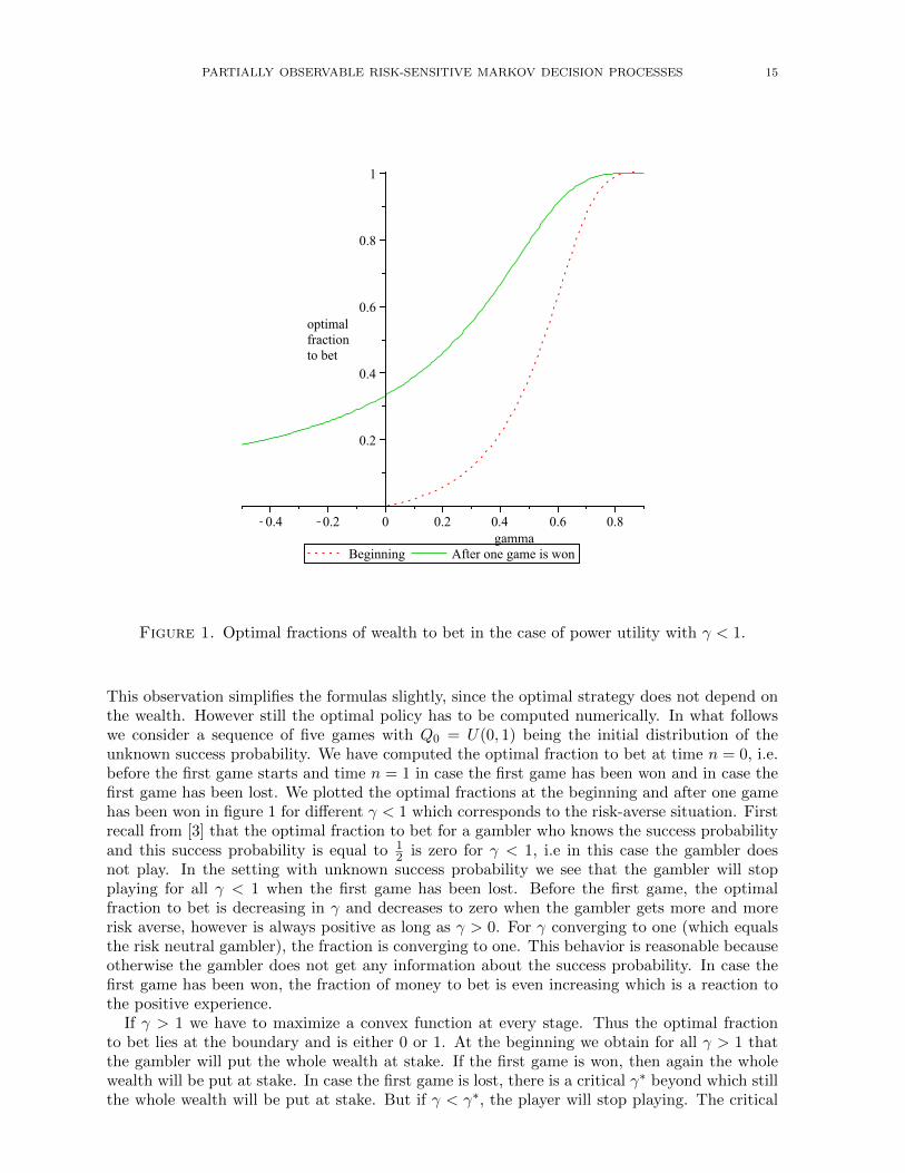
Figure 1. Optimal fractions of wealth to bet in the case of power utility with γ < 1.

This observation simplifies the formulas slightly, since the optimal strategy does not depend onthe wealth. However still the optimal policy has to be computed numerically. In what followswe consider a sequence of five games with Q0 = U(0, 1) being the initial distribution of theunknown success probability. We have computed the optimal fraction to bet at time n = 0, i.e.before the first game starts and time n = 1 in case the first game has been won and in case thefirst game has been lost. We plotted the optimal fractions at the beginning and after one gamehas been won in figure 1 for different γ < 1 which corresponds to the risk-averse situation. Firstrecall from [3] that the optimal fraction to bet for a gambler who knows the success probabilityand this success probability is equal to 1

2 is zero for γ < 1, i.e in this case the gambler doesnot play. In the setting with unknown success probability we see that the gambler will stopplaying for all γ < 1 when the first game has been lost. Before the first game, the optimalfraction to bet is decreasing in γ and decreases to zero when the gambler gets more and morerisk averse, however is always positive as long as γ > 0. For γ converging to one (which equalsthe risk neutral gambler), the fraction is converging to one. This behavior is reasonable becauseotherwise the gambler does not get any information about the success probability. In case thefirst game has been won, the fraction of money to bet is even increasing which is a reaction tothe positive experience.

If γ > 1 we have to maximize a convex function at every stage. Thus the optimal fractionto bet lies at the boundary and is either 0 or 1. At the beginning we obtain for all γ > 1 thatthe gambler will put the whole wealth at stake. If the first game is won, then again the wholewealth will be put at stake. In case the first game is lost, there is a critical γ∗ beyond which stillthe whole wealth will be put at stake. But if γ < γ∗, the player will stop playing. The critical


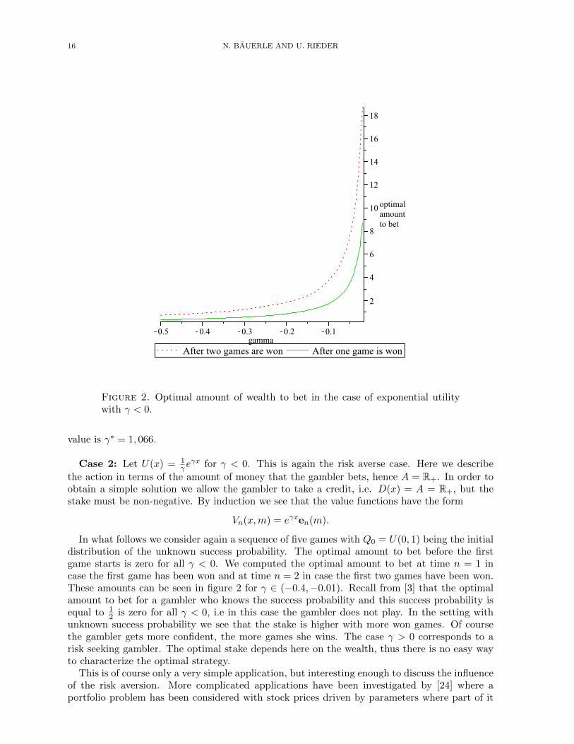
Figure 2. Optimal amount of wealth to bet in the case of exponential utilitywith γ < 0.

value is γ∗ = 1, 066.

Case 2: Let U(x) = 1γ e

γx for γ < 0. This is again the risk averse case. Here we describe

the action in terms of the amount of money that the gambler bets, hence A = R+. In order toobtain a simple solution we allow the gambler to take a credit, i.e. D(x) = A = R+, but thestake must be non-negative. By induction we see that the value functions have the form

Vn(x,m) = eγxen(m).

In what follows we consider again a sequence of five games with Q0 = U(0, 1) being the initialdistribution of the unknown success probability. The optimal amount to bet before the firstgame starts is zero for all γ < 0. We computed the optimal amount to bet at time n = 1 incase the first game has been won and at time n = 2 in case the first two games have been won.These amounts can be seen in figure 2 for γ ∈ (−0.4,−0.01). Recall from [3] that the optimalamount to bet for a gambler who knows the success probability and this success probability isequal to 1

2 is zero for all γ < 0, i.e in this case the gambler does not play. In the setting withunknown success probability we see that the stake is higher with more won games. Of coursethe gambler gets more confident, the more games she wins. The case γ > 0 corresponds to arisk seeking gambler. The optimal stake depends here on the wealth, thus there is no easy wayto characterize the optimal strategy.

This is of course only a very simple application, but interesting enough to discuss the influenceof the risk aversion. More complicated applications have been investigated by [24] where aportfolio problem has been considered with stock prices driven by parameters where part of it


cannot be observed. The aim is here to maximize the long run risk-sensitized growth rate of thewealth process where the exponential utility is used.

6. Infinite Horizon Problems

Here we consider an infinite time horizon and β ∈ (0, 1), i.e. we are interested in

J∞(x) := infσ∈Π

∫EY

Eσxy[U( ∞∑k=0

βkc(Xk, Yk, Ak))]Q0(dy), x ∈ E. (6.1)

We will consider concave and convex utility functions separately.

6.1. Concave Utility Function. We first investigate the case of a concave utility functionU : R+ → R. This situation represents a risk seeking decision maker.

In this subsection we use the following notations

V∞σ(x, µ, z) :=

∫EY

∫R+

Eσxy[U(s+ z

∞∑k=0

βkc(Xk, Yk, Ak))]µ(ds, dy),

V∞(x, µ, z) := infσ∈Π

V∞σ(x, µ, z), (x, µ, z) ∈ E. (6.2)

We are interested in obtaining V∞(x,Q0⊗δ0, 1) = J∞(x). For a stationary policy π = (f, f, . . .) ∈ΠM we write V∞π = Vf and denote

b(µ, z) :=

∫R+

U(s+

zc

1− β

)µS(ds),

b(µ, z) :=

∫R+

U(s+

zc

1− β

)µS(ds), (µ, z) ∈ Pb(EY × R+)× [0, 1].

Then we obtain the main theorem of this section:

Theorem 6.1. The following statements hold true:

a) V∞ is the unique solution of v = Tv in C(E) with b(µ, z) ≤ v(x, µ, z) ≤ b(µ, z) for Tdefined in (3.6). Moreover, TnV0 ↑ V∞, Tnb ↑ V∞ and Tnb ↓ V∞ for n→∞. The valuefunction of (6.1) is given by J∞(x) = V∞(x,Q0 ⊗ δ0, 1).

b) There exists a minimizer f∗ of V∞ and (g∗0, g∗1, . . .) with

g∗n(hn) := f∗(xn, µn(·|hn), βn

)is an optimal policy for (6.1).

Proof. a) We first show that Vn = TnV0 ↑ V∞ for n → ∞. To this end note that forU : R+ → R increasing and concave we obtain the inequality

U(s1 + s2) ≤ U(s1) + U ′−(s1)s2, s1, s2 ≥ 0


where U ′− is the left-hand side derivative of U which exists since U in concave. Moreover,U ′−(s) ≥ 0 and U ′− is decreasing. For (x, µ, z) ∈ E and σ ∈ Π it holds

Vn(x, µ, z) ≤ Vnσ(x, µ, z) ≤ V∞σ(x, µ, z)

=

∫EY

∫R+

Eσxy[U(s+ z

∞∑k=0


≤∫EY

∫R+

Eσxy[U(s+ z

n−1∑k=0


+

∫EY

∫R+

Eσxy[U ′−

(s+ z

n−1∑k=0

βkc(Xk, Yk, Ak))z∞∑m=n

βkc(Xm, Ym, Am)]µ(dy, ds)

≤ Vnσ(x, µ, z) +

∫R+

U ′−(s+ zc)µS(ds)βnzc

1− β

≤ Vnσ(x, µ, z) + U ′−(zc)βnzc

1− β=: Vnσ(x, µ, z) + εn(z), (6.3)

where εn(z) has implicitly been defined in the last equation.Obviously limn→∞ εn(z) = 0. Taking the infimum over all policies in the preceding

inequality yields:

Vn(x, µ, z) ≤ V∞(x, µ, z) ≤ Vn(x, µ, z) + εn(z).

Letting n → ∞ yields Vn = TnV0 ↑ V∞ for n → ∞. Note that the convergence of TnV0

is monotone (see Remark 3.5).By direct inspection we obtain b ≤ V∞ ≤ b. We next show that V∞ = TV∞. Note

that Vn ≤ V∞ for all n. Since T is increasing we have Vn+1 = TVn ≤ TV∞ for all n.Letting n→∞ implies V∞ ≤ TV∞. For the reverse inequality recall that Vn + εn ≥ V∞from (6.3). Applying the T -operator yields Vn+1 +εn+1 = T (Vn+εn) ≥ TV∞ and lettingn→∞ we obtain V∞ ≥ TV∞. Hence it follows V∞ = TV∞.

Next, we obtain

(T b)(µ, z) = infa∈D(x)

∫R+

U(s′ +

zβc

1− β

)ΨS(x, a, x′µ, z)(ds′)

≤∫R+

U(s+ zc+

zβc

1− β

)µS(ds)

=

∫R+

U(s+

zc

1− β

)µS(ds) = b(µ, z).

Analogously Tb ≥ b. Thus we get that Tnb ↓ and Tnb ↑ and the limits exist. Moreover,we obtain by iteration:

(Tnb)(x, µ, z) =

= infπ∈ΠM

∫EY

∫R+

Eπxy[U(s+

zcβn

1− β+ z

n−1∑k=0

βkc(Xk, Yk, Ak))]µ(dy, ds) ≥ (TnV0)(x, µ, z)

(Tnb)(x, µ, z) =

= infπ∈ΠM

∫EY

∫R+

Eπxy[U(s+

zcβn

1− β+ z

n−1∑k=0



Using U(s1 + s2)− U(s1) ≤ U ′−(s1)s2 we obtain:

0 ≤ (Tnb)(x, µ, z)− (Tnb)(x, µ, z) ≤ (Tnb)(x, µ, z)− (TnV0)(x, µ, z)

≤ supπ∈Π

∫EY

∫R+

Eπxy[U(s+

zcβn

1− β+ z

n−1∑k=0

βkc(Xk, Yk, Ak))−

U(s+ z

n−1∑k=0


≤ εn(z)

and the right-hand side converges to zero for n→∞. As a result Tnb ↓ V∞ and Tnb ↑ V∞for n→∞.

Since Vn is lower semicontinuous, this yields immediately that V∞ is again lower semi-continuous, thus V∞ ∈ C(E).

For the uniqueness suppose that v ∈ C(E) is another solution of v = Tv withb ≤ v ≤ b. Then Tnb ≤ v ≤ Tnb for all n ∈ N and since the limit n → ∞ of theright and left-hand side are equal to V∞ the statement follows.

b) The existence of a minimizer follows from our standing assumption (A) as in the proofof Theorem 3.3. From our assumption and the fact that V∞ ≥ V0 we obtain

V∞ = limn→∞

Tnf∗V∞ ≥ limn→∞

Tnf∗V0 = limn→∞

Vn(f∗,f∗,...) = Vf∗ ≥ V∞

where the last equation follows with dominated convergence. Hence (g∗0, g∗1, . . .) is optimal

for (6.1).�

6.2. Convex Utility Function. Here we consider the problem with convex utility U . Thissituation represents a risk averse decision maker. The value functions Vnσ, Vn, V∞σ, V∞ aredefined as in the previous section.

Theorem 6.2. Theorem 6.1 also holds for convex U .

Proof. The proof follows along the same lines as in Theorem 6.1. The only difference is that wehave to use another inequality: Note that for U : R+ → R increasing and convex we obtain theinequality

U(s1 + s2) ≤ U(s1) + U ′+(s1 + s2)s2, s1, s2 ≥ 0

where U ′+ is the right-hand side derivative of U which exists since U in convex. Moreover,U ′+(s) ≥ 0 and U ′+ is increasing. Thus, we obtain for (x, µ, z) ∈ E and σ ∈ Π:

Vn(x, µ, z) ≤ Vnσ(x, µ, z) ≤ V∞σ(x, µ, z)

=

∫EY

∫R+

Eσxy[U(s+ z

∞∑k=0


≤∫EY

∫R+

Eσxy[U(s+ z

n−1∑k=0

βkc(Xk, Yk, Ak))]

+

+Eσxy[U ′+

(s+ z

∞∑k=0

βkc(Xk, Yk, Ak))z

∞∑k=n

βkc(Xk, Yk, Ak)]µ(dy, ds)

≤ Vnσ(x, µ, z) +

∫R+

U ′+

(s+

zc

1− β

)µS(ds)

zcβn

1− β.

Note that the last inequality follows from the fact that c is bounded from above by c. Now

denote δn(µ, z) :=∫R+U ′+

(s+ zc

1−β +)µS(ds) zcβ

n

1−β . Obviously limn→∞ δn(µ, z) = 0. Taking the

infimum over all policies in the above inequality yields:

Vn(x, µ, z) ≤ V∞(x, µ, z) ≤ Vn(x, µ, z) + δn(µ, z).


Letting n→∞ yields TnV0 → V∞.Further we have to use the inequality

0 ≤ (Tnb)(x, µ, z)− (Tnb)(x, µ, z) ≤ (Tnb)(x, µ, z)− (TnV0)(x, µ, z)

≤ supπ∈Π

∫EY

∫R+

Eπx[U(s+

zcβn

1− β+ z

n−1∑k=0

βkc(Xk, Yk, Ak))−

U(s+ z

n−1∑k=0


≤∫R+

U ′+

(s+

zc

1− β

)µS(ds)

zcβn

1− β= δn(µ, z)

and the right-hand side converges to zero for n→∞. �

6.3. Exponential Utility. Of course the result for the infinite horizon problem can now bespecialized to various situations like in Section 4. This can be done rather straightforward. Weonly present the case of the exponential utility due to its importance.

Corollary 6.3. In case U(x) = 1γ e

γx with γ 6= 0, we obtain

a) V∞(x, µ, z) =∫eγsµS(ds)e∞(x, µ, γz), (x, µ, z) ∈ EX ×P(EY ×R+)× (0, 1] where µ has

been defined in (4.2) and the function e∞ is the unique fixed point of

e∞(x, µ, γz) = infa∈D(x)

∫EX

e∞(x′,Ψe(x, a, x′, µ, γz), βγz)QX

(dx′|x, µ, a, γz

),

for (x, µ, z) ∈ EX × P(EY ) × (0, 1] with U( zc1−β ) ≤ e∞(x, µ, γz) ≤ U( zc

1−β ). The value

function of (6.1) is then given by J∞(x) = e∞(x,Q0, γ).b) There exists a minimizer f∗ of e∞ and (g∗0, g

∗1, . . .) with

g∗n(hn) := f∗(xn, µ

en(·|hn), γβn

)is an optimal policy for (6.1), where the sequence (µen) of posterior distributions is gen-erated by the updating operator Ψe with µe0 := Q0 like in Theorem 4.4.

References

[1] M. Aoki, Optimal control of partially observable Markovian systems. Journal of TheFranklin Institute 280(5), 367-386, (1965).

[2] N. Bauerle and U. Rieder, Markov Decision Processes with Applications to Finance.Springer-Verlag, Berlin Heidelberg, (2011).

[3] N. Bauerle and U. Rieder, More risk-sensitive Markov Decision Processes. Mathematics ofOperations Research 39(1), 105-120, (2014).

[4] N. Bauerle and A. Jaskiewicz, Risk-sensitive dividend problems. European Journal of Op-erational Research 242(1), 161-171, (2015).

[5] A. Bensoussan, Stochastic control of partially observable systems. Cambridge UniversityPress, (2004).

[6] T. Bielecki and S. Pliska, Economic properties of the risk sensitive criterion for portfoliomanagement. Review of Accounting and Finance (2), 3-17, (2003).

[7] R. Cavazos-Cadena and D. Hernandez-Hernandez, Successive approximations in partiallyobservable controlled Markov chains with risk-sensitive average criterion. Stochastics 77(6),537-568, (2005).

[8] R. Cavazos-Cadena and D. Hernandez-Hernandez, A Characterization of the Optimal Cer-tainty Equivalent of the Average Cost via the Arrow-Pratt Sensitivity Function. Math OperRes (to appear), (2015)

[9] M.H.A. Davis and Sebastien Lleo, Risk-Sensitive Investment Management. World Scientific,(2014).


[10] Di Masi and L. Stettner, Risk sensitive control of discrete time partially observed Markovprocesses with infinite horizon. Stochastics 67(3-4), 309-322, (1999).

[11] J. Fan and A. Ruszczynski. Process-Based Risk Measures for Observable and PartiallyObservable Discrete-Time Controlled Systems. arXiv:1411.2675 (2014).

[12] E. Feinberg and P. Kasyanov and M. Zgurovsky, Convergence of probability measrues andMarkov Decision Models with Incomplete Information. arXiv:1407.1029v1, (2014).

[13] E. Feinberg and P. Kasyanov and M. Zgurovsky, Partially observable total-cost Markov De-cision Processes with weakly continuous transition probabilities. arXiv:1401.2168v2, (2014).

[14] W. Fleming and D. Hernandez-Hernandez, Risk-sensitive control of finite state machines onan infinite horizon II. SIAM journal on control and optimization 37(4), 1048-1069, (1999).

[15] W.B. Haskell and R. Jain, A convex analytic approach to risk-aware Markov DecisionProcesses. Preprint (2014).

[16] D. Hernandez-Hernandez, Partially observed control problems with multiplicative cost,In: Stochastic Analysis, Control, Optimization and Applications. Birkhauser Boston,41-55, (1999).

[17] O. Hernandez-Lerma, Adaptive Markov control processes. Springer-Verlag, (1989).[18] K. Hinderer, Foundations of non-stationary dynamic programming with discrete time pa-

rameter. Springer-Verlag, Berlin, (1970).[19] R.A. Howard and J.E. Matheson, Risk-sensitive Markov Decision Processes. Management

Science (18), 356–369, (1972).[20] M.R. James and J.S. Baras and R.J. Elliott, Risk-sensitive control and dynamic games

for partially observed discrete-time nonlinear systems. IEEE Transactions on AutomaticControl 39(4), 780-792, (1994).

[21] P.R. Kumar and P. Varaiya, Stochastic systems: Estimation, identification, and adaptivecontrol. Englewood Cliffs, NJ: Prentice Hall, (1986).

[22] D. Rhenius, Incomplete information in Markovian decision models. The Annals of Statistics,1327-1334, (1974):

[23] W. Runggaldier and L. Stettner, Approximations of discrete time partially observed controlproblems. Applied Mathematics Monographs 6, Giardini Editori, Pisa, (1994).

[24] L. Stettner, Risk sensitive portfolio optmization with completely and partially observedfactors. IEEE Transactions on Automatic Control 49(3), 457-464, (2004).

[25] P. Whittle, Risk-sensitive linear quadratic Gaussian control. Advances in Applied Proba-bility 13, 764-777, (1981).

[26] A.A. Yushkevich, Reduction of a Controlled Markov Model with Incomplete Data to aProblem with Complete Information in the Case of Borel State and Control Space. Theoryof Probability & Its Applications 21(1), 153-158, (1976).

(N. Bauerle) Institute for Stochastics, Karlsruhe Institute of Technology, D-76128 Karlsruhe,Germany

E-mail address: [email protected]

(U. Rieder) University of Ulm, D-89069 Ulm, GermanyE-mail address: [email protected]

mailto:[email protected]

mailto:[email protected]

partially observable risk-sensitive markov decision processes

Documents