papua new guinea poverty and access to public services
TRANSCRIPT

Report No. 19584-PNG
Papua New GuineaPoverty and Access to Public Services
February 18, 2000
FOR OFFICIAL USE ONLY
Document of the World Bank
This document has a restricted distribution and may be used by recipientsonly in the performance of their official duties. Its contents may not otherwisebe disclosed without World Bank authorization.
Pub
lic D
iscl
osur
e A
utho
rized
Pub
lic D
iscl
osur
e A
utho
rized
Pub
lic D
iscl
osur
e A
utho
rized
Pub
lic D
iscl
osur
e A
utho
rized
Pub
lic D
iscl
osur
e A
utho
rized
Pub
lic D
iscl
osur
e A
utho
rized
Pub
lic D
iscl
osur
e A
utho
rized
Pub
lic D
iscl
osur
e A
utho
rized

CURRENCY EQUIVALENTS(As of October 11, 1999)
Currency Unit = Kina (K)$1.00 = K3.13K 1.00 $0.32
ABBREVIATIONS
GOPNG Government of Papua New GuineaNCD National Capital DistrictPNG Papua New GuineaNGO Non-Government OrganizationPSU Primary Sampling UnitCU Census UnitNSO National Statistical OfficeCARP Cluster Analysis and Regression Package
Vice-President: Jean-Michel Severino, EAPVPCountry Director: Klaus Rohland, EACNISector Manager: Homi Kharas, EASPRTask Manager: Monika Huppi, EASPR
FOR OFFICIAL USE ONLY
PAPUA NEW GUINEAPOVERTY AND ACCESS TO PUBLIC SERVICES
CONTENTS
Page No.Executive Summary ....................................... v
Background ....................................... vPoverty Profile ...................................... vPoverty and access to public services ...................................... viSocial Safety Nets ...................................... ix
Information gaps and need for further analysis ....................................... x
1. Assessing Poverty in PNG ..A. Background .IB. Per capita consumption, distribution and inequality .3C. Measuring poverty in PNG .5
2. Poverty And Access To Public Services .. 17A. Introduction .17B. Health and Nutrition .18C. Education and Literacy .26D. Rural Infrastructure .35E. Living Standards and Access to Public Services .38F. Decentralization and Provision of Basic Services ..................................... 38
3. Social Safety Nets .. 42A. Introduction .42B. Informal Social Safety Nets .42C. Formal Social Safety Nets .46
4. Information Gaps and Future Analysis to Guide Poverty Alleviation Policies.. 50A. Information Gaps and Additional Analysis .50B. Lessons from the 1996 Household Survey .52
Bibliographic References .................. 55
This document has a restricted distribution and may be used by recipients only in the performance oftheir official duties. Its contents may not otherwise be disclosed without World Bank authorization.
PAPUA NEW GUINEA: POVERTY AND ACCESS TO PUBLIC SERVICES
Annexes
I . Measuring the Standard of Living .............................................................. 602. Setting A Poverty Line .............................................................. 973. Effect of Using Sampling Unit Specific Prices and Urban/Rural Price ..................... 110
Differentials in Poverty Lines4. Determinants of Child Growth .............................................................. 1155. Decomposing the Gender Gap in Primary School Enrolment .................................. 1196. Multivariate Analysis of Poverty in Papua New Guinea ........................................... 1267. Private Transfers and the Social Safety Net in Papua New Guinea ........................... 141
Tables in Text
1.1 Comparative Social Indicators .............................................................. 11.2 Relative Importance of Economic Sectors and Labor Force Distribution ................... 21.3 Consumption Across Income Groups and Regions ...................................................... 41.4 Regional Poverty Lines .............................................................. 61.5 Poverty Measures by Region .............................................................. 81.6 Poverty by Household Size, Age and Gender of Household Head ........................... 121.7 Poverty by Educational Attainment of Household Head ........................................... 121.8 Incidence and Severity of Poverty by Main Income Source of Household Head ...... 141.9 Poverty and Income Sources for Working Age Adults .............................................. 16
2.1 Distribution Of Social Indicators Across Expenditure Groups .................................. 172.2 Perceptions about Adequacy of Public Services ....................................................... 182.3 Comparative Health Indicators .............................................................. 192.4 Distribution and Condition of Health Care Facilities across Provinces .................... 202.5 Access to Health Facilities and Medical Expenditures by Consumption Quartile .... 212.6 Contacts with Health Care Facilities by Consumption Quartile ............................... 212.7 Source of Drinking Water and Sanitation by Consumption Level ............................ 232.8 The Distribution of Stunting in Young Children ....................................................... 242.9 The Distribution of Wasting in Young Children ....................................................... 252.10 Anthropometric Indicators for Adults ........................ ...................................... 262.11 Adult Literacy Rates and Gender Gaps by Region .................................................... 272.12 Distribution of Schooling ..................... 282.13 School Enrolment Ratios in PNG and EAP ....................................... 292.14 Net Enrollment Rates at Primary and Secondary School Level . . 302.15 Distribution of (within-year) School Drop-Outs by Schooling Level .. 312.16 Distribution of Reasons for Dropping-Out ........................................ 322.17 Average Travelling Time to Schools ............................................ 322.18 Access to Public Transportation ..................................................... 362.19 Simulated Effect of Certain Changes on Incidence of Poverty . . 39
ii

POVERTYAND ACCESS TO PUBLIC SERVICES
3.1 Percentage of Households Giving and Receiving Private Inter-household .............. 43Cash and in-Kind Transfers in Papua New Guinea
3.2 Average Value of Private Inter-household Cash and in-Kind Transfers as ............. 44a Percentage of Total Household Expenditure in Papua New Guinea
Figures in Text
1.1 Growth in Real GDP, Formal Employment and Labor Force: 1980-1995 ................. 21.2 Regional Contribution to National Poverty ............................................................ 91.3 Headcount Index and Contribution to Poverty by Agro-ecological Region ............. 112.1 Adult Literacy Rates by Sex and Consumption Quartile ....................... ................... 272.2 Contribution to National Poverty by School Attainment of Household Head .......... 282.3 Educational Attainment Across Regions ........................................................... 282.4 Affordability of Education ........................................................... 332.5 Consumption and Access to Transportation ........................................................... 36
Boxes in Text
1. Inequality Comparisons .52. International Poverty Comparisons .103. Summary Profile of Poor Households .144. Summary Profile of Poor Households by Region .155. Decentralization, Redistribution and the Provision of Social Services .416. Benefits Incidence of Public Expenditures on Health and Education .51
in Vietnam and Malaysia
iii

POVERTYANDACCESS TO PUBLICSERVICES
Acknowledgements
This report was prepared by Monika Huppi and John Gibson under the direction ofKlaus Rohland, Country Director for Papua New Guinea. It has benefited from the comments andinputs of Martin Ravallion, Robin Hide, Tamar Manuelyan-Atinc, Gaurav Datt, Lionel Demery,Bruce Harris, Norbert Schady and Cyrus Talati.
The report is largely based on the 1996 Household Survey and a number of backgroundstudies-on agriculture, health, education, social safety nets, and NGOs-which were managed byDavid Klaus.
The household survey was the first ever for Papua New Guinea and would not have beenpossible without the funding that was provided by the Governments of Australia, Japan, NewZealand, and the World Bank.
A large number of institutions and individuals were involved in the preparation andimplementation of the survey and background studies. These include John Gibson of the Universityof Waikato, Scott Rozelle of Stanford University, the late Christopher Scott, B.J. Allen andR.M. Bourke Allen of Australian National University, Carol Jenkins of the Institute of MedicalResearch, Richard Guy, Pani Tawaiyole, John Khambu, Wari lamo, Agogo Mawuli, of the NationalResearch Institute, John Millet of the Institute of National Affairs, Education Development Centre,Michael French Smith, Micael Olsson, and Malcolm Levett and Unisearch of the University ofPapua New Guinea.
Iv
PAPUA NEW GUINEA: POVERTY AND ACCESS TO PUBLIC SERVICES
EXECUTIVE SUMMARY
BACKGROUND
1. At an average annual income of US$890 per capita (1998), Papua New Guinea (PNG) isclassified as a lower middle-income country. Compared to other countries in this group and inthe East Asia and Pacific region, PNG scores poorly with respect to basic social indicators. Thissuggests that an important share of PNG's population may be less well off than the country'sincome level would imply.
2. This report analyzes the distribution of income, constructs a poverty profile and looks atthe extent to which the poor have access to basic services. The analysis is based on data collectedduring a national household survey in 1996. This was the first and only multipurpose andnationally representative household survey carried out in PNG. Data on a range of social andeconomic indicators were collected from a nationally representative sample of 1,200 householdsrepresenting urban and rural households and PNG's five major regions (National Capital District,Papuan/South Coast, Highlands, Momase/North Coast, New Guinea Islands).
3. Distribution of Consumption. The household survey data show that consumption isvery unevenly distributed in PNG. The wealthiest 25 percent of the population have a real percapita consumption level over eight times higher than the poorest quartile. There are also markeddisparities in consumption levels across regions. Overall, the distribution of consumption in PNGis more unequal than in most countries with comparable income levels. The Gini coefficientderived from the household expenditure data (adjusted for spatial price variations and adultequivalent consumption) is 0.46.
POVERTY PROFILE
4. Poverty Line. To measure poverty based on household consumption, a minimumacceptable level of consumption (a poverty line) needs to be determined which separates the poorfrom the non-poor. PNG does not have an official poverty line. The poverty lines used in thisreport are based on the cost of a food consumption basket which meets a minimum food -energyrequirement of 2,200 calories per adult equivalent per day and reflects the dietary pattern of thelower income groups (food-poverty line). Food expenditures are supplemented by an allowancefor non-food expenditures based on the expenditure pattern of those households whose foodexpenditures just reach the food-poverty line. This results in an average national poverty line of461 kina per adult equivalent per year. A second, somewhat lower poverty line (399 kina peradult equivalent per year) is based on the same food expenditures, but contains a more restrictedallowance for non-food expenditures based on the non-food expenditure share and consumptionpattern of those households whose overall expenditures reach the food-poverty line. Becausethere are significant spatial price variations across PNG, the report calculates separate povertylines for each one of the five major regions used in the analysis.
v
POVERTYAND ACCESS TO PUBLIC SER VICES
5. Level and Distribution of Poverty. Based on an average national poverty line of 461kina per adult equivalent per year (1996 prices), about 37 percent of PNG's population must beconsidered as poor. The vast majority (93 percent) of those who are poor live in rural areas,where over 41 percent of the population fall below the poverty line. This compares to aheadcount index of poverty of just 16 percent for urban areas. Poverty is highest in theMomase/North Coast region (46 percent), but in absolute terms, the highest number of poorhouseholds live in the Highlands region. The poor in the Highlands account for 38 percent ofPNG's poor. Poverty is lowest in the National Capital District (NCD) (just under 26 percent) andthe poor in this region account for less than 4 percent of the country's poor. The report alsomeasures poverty in PNG at an international poverty line of US$ 1/capita/day (1985 prices)converted at the purchasing power parity exchange rate and finds that poverty levels in PNG arehigh compared to other countries with similar income levels.
6. Who are the poor? Over 93 percent of the poor live in rural areas. Many of them do notearn any cash income and thus derive their livelihood almost entirely from subsistenceagriculture. Of those who earn cash income, poverty is highest among those engaged in smallscale tree crop production, domestic agriculture and hunting - gathering. Tree crop producers arethe most important group in terms of contribution to national poverty and account for 42 percentof PNG's poor. Poverty is significantly lower among households whose head does not depend onagriculture, fishing, hunting or gathering as a main income source. Those households whose headhave a formal sector wage job register the lowest incidence of poverty (17 percent), followed bythose whose head runs a business (25 percent). Poverty is more widespread among householdswith older heads and among those who have not attended school. The gender of a householdhead does not appear to be a good predictor for poverty, as differences in poverty measuresbetween female- and male-headed households are not statistically significant.
POVERTY AND ACCESS TO PUBLIC SERVICES
7. Data from the household survey show that lower expenditure groups in PNG faresignificantly worse than the upper groups across a wide range of social indicators. Because mostof these indicators are substantially influenced by access to basic services such as education,health care, rural infrastructure and utilities, the report reviews distribution of access to suchservices in more detail. Unequal access to health, education, transport facilities and utilities canfurther accentuate the effects of unequal income distribution.
8. The household survey shows that there is a clear positive correlation between the level ofconsumption and a person's satisfaction with his family's access to public services, such ashealth care, education and transport facilities. This suggests that the upper income groups benefitfrom better access to basic public services than the poor. It is, however, striking that PNG'spopulation overall shows a very low level of satisfaction with the provision of basic socialservices. Over half the population consider that their children do not get appropriate access toschooling, almost 60 percent consider their access to health care unsatisfactory and two thirds ofthe population express dissatisfaction with their access to public transportation.
vi
POVERTYAND ACCESS TO PUBLIC SER VICES
Health Services
9. Although PNG has a relatively well developed health care infrastructure, the health andnutritional status of its population compares unfavorably to that of other countries in the regionand has stagnated over the past decade. The low health standards point to unsatisfactoryperformance and substantial inefficiencies of PNG's health care system.
10. The three tier community based health care system with aid posts serving the ruralpopulation, health centers at the next level and hospitals at the tertiary level which PNG inheritedat independence has ceased to function properly. The drop in the quality of health servicesavailable in rural areas has been particularly severe due to the increasing bias towards urbanbased curative care. Among the reasons for the increasingly poor performance of PNG's healthcare system are: (i) growing personnel expenditures which crowd out other operationalexpenditures; (ii) an erratic flow of funds which makes it impossible to properly plan and executepriority health programs; (iii) low skill levels among health workers and sectoral managers; (iv) abreakdown of the supervision and referral system where higher order facilities provide guidanceand supervision to lower end facilities and; (v) an unclear division of responsibilities betweenlocal and central Government agencies with respect to management and supervision of the healthsector.
11. Access to health facilities by lower income groups is substantially inferior to that of theupper income groups. People from the lowest consumption quartile travel more than twice aslong to reach an aid post or a health care center than those among the top consumption quartile.Lower income groups make much less use of formal health care providers than the upper groupsand they appeal almost exclusively to lower end facilities (aid posts and health centers). On theother hand, almost one third of all contacts by the top consumption quartile are with a hospital,where the quality of service remains substantially better than in the lower end facilities.
12. Households ranked improved access to health care among the highest priorities for publicintervention and NGO assistance. Reform of PNG's health care system is critical to improve thepopulation's health standards and raise the lower income groups' access to proper health care.
13. Water and Sanitation. Availability of clean water and appropriate sanitation has animportant bearing on the population's health status. Over 60 percent of the population rely onrivers, lakes, creeks and similar unprotected sources for drinking water. The poor are particularlyat risk for unsafe water. Not surprisingly, improvements in access to safe water was ranked asone of the highest priorities by households and the Government should make provision of safewater a main concern in the area of public health.
14. Poverty and Malnutrition. Malnutrition is a considerable problem among PNG'spopulation, particularly among women and children. It is closely linked to poverty. The risks ofchildren and women from the lower consumption quartiles being chronically malnourished aresignificantly higher than those of children and women from the upper quartiles.
vii

POVERTYAND ACCESS To PUBLICSERVICES
Schooling and Literacy
15. Literacy. Literacy and schooling are key determinants of a person's ability to takeadvantage of income-earning opportunities. Literacy rates remain low in PNG and there is amarked gender gap in literacy achievement. Based on the household survey, only 63 percent ofPNG's men and 44 percent of PNG's women consider that they are literate. Literacy rates and thegender gap vary widely between regions. Literacy rates drop significantly with decreasingincome levels.
16. Educational Attainment. Only half of all women aged 15 and above and two thirds ofmen have ever attended school. Educational attainment in PNG is strongly related to economicwelfare. Over half of all poor in PNG live in households whose head has never attended school,although this group only accounts for 38 percent of the population. There are also markeddisparities in the regional distribution of educational attainment. The proportion of the adultpopulation who have never attended school ranges from a moderate 15 percent in the urban NCDto a high 57 percent in the Highlands.
17. School Enrolments. School attendance among PNG's children remains low. Netenrolment rates are 51 percent for primary school age children and 17 percent for secondaryschool age children, according to the household survey. The gender gap in school enrolmentsincreases with decreasing consumption levels. Enrolment rates vary significantly across regions:less than one half of all primary-school age children in the Highlands are in primary school,while the NCD and New Guinea Islands achieve enrolment rates of 76 percent and 68 percentrespectively.
18. The lack of access to proper schooling by children of the lower income groups is drivenby several factors, including a need to travel long distances to schools, particularly secondaryschools; lack of teachers in remote areas; and an inability to meet educational expenditures.
19. GOPNG has recently launched a major education sector reform program. The programaims to achieve universal coverage of basic education, to improve system efficiency and toincrease girls' participation in education. The program has made a good start. But its initialsuccess now threatens to be tempered by growing capacity constraints at the central and theprovincial levels and limited availability of resources. Overall budgetary constraints make itunlikely that substantial additional resources will be available to finance the continuedimplementation of the education reform program. Therefore, measures which substantially raisethe internal efficiency of PNG's education system, such as a reduction in drop-out rates andmore efficient deployment of teachers, will be essential to the continued successfulimplementation of the program. An intra-sectoral shift in resource allocation away from highereducation towards basic education should accompany efficiency improvements. Successfulimplementation of the program will be essential for poverty alleviation in PNG.
viii

POVERTYAND ACCESS TO PUBLIC SER VICES
Rural Infrastructure
20. Access to transport infrastructure is an important determinant of economic welfare inPNG. The household survey has shown that there is a marked difference in access totransportation infrastructure between income groups. The lowest consumption quartile musttravel over twice as long to gain access to the closest mode of transport than the richest quartile.
21. Although PNG compares relatively favorably with other developing countries in terms ofmeters of road per person and per square kilometer, a vast majority of roads are poorlymaintained and inaccessible during and after rains. Together with the poor integration ofdifferent modes of transportation (road, water, air), this results in a highly fragmented andunreliable transportation system and high transportation costs. The latter in turn increasesmarketing costs and limits possibilities of market integration.
22. Investments in rural infrastructure (roads, shipping facilities, markets, water supply) arecritical to spur broad-based rural development and alleviate poverty in PNG. First priority shouldbe given to rehabilitate existing roads and to assure subsequent proper maintenance. Thecountry's difficult topography and terrain will make it impossible to provide all areas with easy,year-round access to transportation. Apart from modest investments in rural tracks, investmentsin new transportation facilities should be carefully considered for their economic viability.Substantial investments in isolated areas with very low population densities may well not turnout to be economically viable. A policy that over time encourages out-migration from such areasmay be a more effective means to alleviate poverty. In the short run, alternative interventionsaimed at alleviating poverty are needed in such areas. Among them are improved access to basiceducation and health services and small scale infrastructure investments that help facilitate livingconditions.
23. To properly target small scale infrastructure investments and assure effectiveparticipation by the local communities, local investment fund arrangements should beconsidered. Such funds would provide financing for small scale investments to communitieswilling to participate and contribute to a particular project of importance to them. Operation ofsuch funds could conceivably be modeled on the functioning of Social Investment Funds whichhave successfully helped alleviate poverty and mobilize local communities in many parts of theworld.
SOCIAL SAFETY NETS
24. PNG has an extensive informal safety net system. This system allows for incometransfers and other support from members of a particular wantok (informal network based onkinship, ethnicity, language or sometimes merely friendship) to needy members of the samewantok system. The household survey has found that inter-household income transfers remain avery important means of assisting households in need across all income groups, althoughinformal income transfers do not appear to improve the income distribution in rural areas. Thewantok system has adapted relatively well to changing economic and social environments and
ix
POVERTYAND ACCESS To PUBLiC SER VICES
remains as important in urban as in rural areas. Wantoks may, however, be limited in theireffectiveness in communities characterized by very high poverty rates or in times of shock,particularly those brought about by natural disasters. There is therefore a need to supplementthese informal safety nets with interventions such as targeted income transfers (e.g., targetedprovision of subsidized health and education services) and improved provision of governmentand NGO funded emergency and relief services. The establishment of self-targeted workfareschemes should also be explored as a means to help alleviate poverty. Such schemes wouldprovide publicly financed unskilled work on demand at a wage rate low enough to guarantee thatonly those in real need are willing to participate. The labor would be used to build and maintainhigh priority community infrastructure in poor areas.
25. PNG's wage linked social insurance schemes, although only benefiting a small part of thepopulation, are an important safety net mechanism and will grow in importance as the countrywill develop further and a larger share of the labor force will enter the formal labor market aswage earners. However, their future effectiveness will largely depend on the Government'sability to implement a series of measures which can strengthen the financial performance of thesefunds.
INFORMATION GAPS AND NEED FOR FURTHER ANALYSIS
26. Further analysis. The data collected during the first nationally representative householdsurvey has made it possible to produce a poverty profile for PNG and to see to what extent thelower income groups have access to basic social services. However, to effectively guideGovernment interventions in favor of poverty alleviation, additional analysis which was notundertaken in this report because of information gaps will be required. This includes a betterunderstanding of the factors which hinder productivity increases and income diversification oflow income agricultural producers; a detailed analysis of the evolution, intra-sectoral allocationand benefits-incidence of public expenditures on health and education, and an evaluation of theimpact of macro-economic policies on the evolution of poverty.
27. Poverty monitoring and lessons from the household survey. To assess the progressmade with respect to poverty alleviation and the effectiveness of Government policies designedto improve the welfare of the poor, regular analysis of the poverty situation is needed. Thisrequires that household surveys be carried out at regular time intervals. PNG should aim atrepeating the household living standard survey within two years of the upcoming PopulationCensus. This would allow to effectively draw on the Census as a sample frame and benefit fromthe capacity build-up at the National Statistics Office. Because an important purpose of the nexthousehold survey will be to see whether poverty has decreased since the last survey, it will beimportant to maintain comparability of data collection methods and a similar coverage for theconsumption aggregate and other indicators of living standards. The ultimate goal of ahousehold survey in PNG should be to have a sample large enough to allow for provincialpoverty profiles. As a next step, a sample large enough to at least allow for separation of urbanand rural sectors in the five main regions should be used. The next survey should also include
x

POVERTYANDACCESS To PUBLICSERVICES
information on land holdings and utilization, access to agricultural support services, credit andmarkets and the quality of basic public services.
xi


PAPuEA NEw GUIEA.- POPERTYA,vD ACCESS TO PUBLiC SERI'ICES
1. ASSESSING POVERTY IN PNG
A. BACKGROUND
1.1 Although Papua New Guinea (PNG) is classified as a lower middle income country withan average annual per capita income of about US$890, the living standard of the vast majority ofits population is akin to that in low-income countries. PNG scores poorly on most socialindicators compared to its income level (Table 1.1). This suggests that the fruits of economicgrowth may have been unevenly distributed and that poverty remains an important developmentproblem in PNG.
Table 1.1: Comparative Social Indicators
Lower-Middle East-Asia andIndicator PNG Income Countries Pacific Region
Infant mortality (per 1000 life birth) 61 38 57Life expectancy at birth 58 68 69Primary school enrolment (gross) 80 103 117% of population with access to 22 58 29adequate sanitation
GNP/Capita (1998 US$/cap) 890 1710 990
Source: World Bank, World Development Indicators, 1998.
1.2 PNG is a nation rich in natural resources, with gold, copper and agricultural productscomprising the most important sources of export earnings. PNG's economic development in thetwo decades since independence has been driven by a small modem enclave sector, mainly basedon mineral resource extraction, commercial logging and tree crop plantations. Governmentpolicies have almost exclusively focussed on fostering the development of these activities.Because it is heavily based on natural resource extraction and plantation agriculture, theperformance of PNG's economy is substantially driven by that of world market commodityprices. Overall, PNG's enclave economy experienced significant but fluctuating growth in outputand exports throughout the last two decades, with little impact on the rest of the economy,particularly the agriculture sector.
1.3 The strong focus on the enclave sector, particularly capital intensive mineral extraction,has done little to create employment opportunities outside subsistence agriculture. Whileindustry and manufacturing account for 40 percent of PNG's value added, they provide
1

POVERTYAND A CCESS To PUBLIC SER vICES
employment for only seven percent of the population. Agriculture, accounting for about onequarter of the country's value added, continues to provide a livelihood for almost 80 percent ofthe population. However, only about 4 percent of the economically active rural population areengaged in modem plantation based agriculture. The remaining 96 percent are village smallholders and many of them are engaged in subsistence or semi-subsistence production.
Table 1.2: Relative Importance of Economic Sectors and Labor Force Distribution
Share in GDP (°) Share in Labor Force (%) Average Annual GDP Growth Rate Share in Labor Absorption1980-96 (%) 1980-96 (%)
Agriculture Industry a Services Agriculture Industry Services Agriculture Industry Services Agriculture IndustTy Service
1980 33 27 40 83 5 12
1996 26 40 33 79 7 14 1.8 5.7 3.1 64 14 22
aIndusty includes manufacturing. Manufacturing accounted for 10 percent and for 8 percent of GDP in 1980 and1996, respectively. It grew by an annual average rate of 1.7 percent between 1980 and 1996. This underlinesthe importance of the mining sector in industry.
Source: World Development Indicators, 1998.
Figure 1.1: Growth in Real GDP, Formal Employment andLabor Force: 1980-1995
1.4 Rigid labor marketpolicies, such as high minimum 4000
wages, have contributed to very 3500
slow employment creation, thus 3000 -
requiring a large share of the 2500 - +Real GDPpopulation to remain in near 2000 - -Employment
subsistence agriculture. Although 1500 \ Labour Force
growth in the agricultural sector 1000 \was substantially below that in 5000the industrial and service sectors 1980 1985 1990 1995 1997
between 1980 and 1996,agriculture absorbed almost twothirds of new entrants in the labor market during this time. Industry (including manufacturing)and services created only 14 percent and 22 percent respectively of new jobs between 1980 and1996. Sluggish performance of the agricultural sector throughout the 1980s, partly due to policiesbiased against agriculture, resulted in little employment generation in rural areas. As a result,open and disguised unemployment have continued to increase substantially, with income levelsfor the majority of the population stagnating.
1.5 Poverty alleviation remains a major development challenge in PNG over the years tocome. To guide Government policy in this direction, it is important to gain insights into theextent and distribution of poverty and to learn what characterises the poor. This report draws up anational poverty profile that can support GOPNG's efforts to improve the design of its poverty
-2-

POVERTY AND ACCESS To PUBLICSERVICES
reduction policies. It also looks at how provision of basic public services and overalldevelopment policies to date have affected the poor.
1.6 Chapter one describes the level and distribution of household consumption, based on datacollected during the 1996 household survey and presents a poverty profile. Chapter two focuseson the access of the poor to basic public services, such as health, education and infrastructure. Italso explores what the impact of improved access to public services would be on poverty levelsin PNG. Chapter three reviews formal and informal safety nets. Chapter four outlines furtherwork that should be carried out to guide GOPNG's future efforts on poverty alleviation andsummarizes the lessons learned from the 1996 household survey.
1.7 The analysis in this report is mainly based on data collected during a national householdsurvey carried out in 1996. The survey collected infornation on a wide range of householdcharacteristics, including demographics, employment, consumption, wealth accumulation, accessto basic public services, anthropometrics and perception of quality of life. This was the firstsurvey to draw on a nationally representative sample of 1200 households. The sample coversurban and rural households in PNG's five major regions (National Capital District, Papuan/SouthCoast, Highlands, Momase/North Coast, New Guinea Islands). Annex 1 provides a more detaileddescription of the household survey.
B. PER CAPITA CONSUMPTION, DISTRIBUTION AND INEQUALITY
1.8 Consumption. Per capita consumption is often used as a basic indicator to measurewelfare. To correctly depict living standards, particularly for purposes of comparing livingstandards across various groups, household expenditure data should be adjusted to capturedifferences in needs and in prices faced by various households. Typically, the cost of sustaining achild is lower than the cost of sustaining an adult. It is therefore sensible to present consumptiondata on an adult equivalent basis, meaning that a smaller weight is given to the cost of childrenthan to that of an adult. Analysis of the household survey consumption data for PNG suggeststhat the cost of supporting a child between ages 0-6 years is in the area of 50 percent of the costsof sustaining an adult, while the costs of a child 7 years and above are close to those of an adult(see Annex 1). Therefore, an adult equivalent adjustment of 0.5 was used for children below 6years of age, while children above that age were given the same weight as adults. Because pricesvary significantly across PNG's regions, household consumption was also adjusted for spatialprice variation. This permits a comparison of consumption across households from various partsof the country (see Annex 1).
1.9 Estimates from the PNG household survey show that nominal per capita consumption peradult equivalent amounted to about 912 kina per year in 1996 (US$ 700). There are, however,significant inter -and intra-regional variations. In nominal terms, adult equivalent per capitaconsumption in the urban National Capital District (NCD) amounts to over three times as muchas that in the poorest New Guinea Islands region. Even after adjustment for spatial pricevariations, marked inter-regional variations in per capita consumption remain. Consumption peradult equivalent in the NCD still amounts to almost twice as much as that in the poorest New
-3-

POVERTYAND ACCESS To PUBLIC SER VICES
Guinea Islands region and to 1.4 times as much as the national average. This points to a markeddifference in the level of welfare between the urban capital region and the predominantly ruralrest of the country. Other inter-regional differences in mean consumption are less marked and notalways statistically significant, because of large intra-regional dispersions around the mean.
1.10 Papua New Guinean households spend a relatively high share of their expenditures onfood (63 percent), suggesting an overall low standard of living. Average caloric availability peradult equivalent is almost 3,000 calories per day and thus well above the often used 2,200minimum caloric requirement. Average protein intake of 55 grams/day/adult equivalent is alsowell over the often suggested minimum requirement of 45 grams/day. These relativelyfavourable national averages mask, however, a very strong variation in food intake across incomegroups.
1.11 Distribution. There are very marked disparities in the distribution of per capitaconsumption across expenditure groups. The wealthiest 25 percent of the population have a realper capita consumption level over eight times higher than the poorest quartile. Average caloricavailability for the poorest 25 percent of the population falls short of the daily requirement and sodoes the protein intake for the poorest 50 percent of the population. This marked disparity innutritional intake between income groups reflects a diet of the lower expenditure groups which isdominated by tubers and starchy staples, but poor in grains, animal fats and proteins.
Table 1.3: Consumption Across Income Groups and Regions.Consumption per adult Consumption per adultequivalent per year (kina) equivalent per dayNominal Real (1) Food share Calories Protein (g)
Consumption quartileI (poorest) 248 258 0.67 1955 27II 457 464 0.67 2587 41III 814 781 0.65 3158 60IV (richest) 2135 2127 0.55 4200 94
RegionNational Capital District 2401 1226 0.50 2697 82Papuan/South Coast 1118 902 0.68 3326 70Highlands 838 860 0.60 2868 48Momase/North Coast 706 1007 0.67 3101 53New Guinea Islands 680 642 0.66 2685 54Total PNG 912 907 0.63 2974 55
Note: (1) Deflated by spatial price deflators, see Annex I
Source: PNG Household Survey 1996
1.12 The distribution of consumption in PNG is more unequal than in most countries withcomparable income levels. The richest 10 percent of the population account for 36 percent ofmeasured consumption, while the poorest 50 percent account for only 20 percent ofconsumption. The Gini coefficient derived from the household survey consumption data is a
-4-

POVERTYAvD ACCESS TO PUBLICSERVICES
high 46.1. For comparison purposes the Gini index was also calculated without adjustingconsumption for spatial price variations and adult equivalencies. This results in a Gini of 48.4,which is significantly higher than that of other countries in the region and of other countrieswith similar per capita incomes (Box 1).
C. MEASURING POVERTY IN PNG
Setting a Poverty Line
1.13 Food Poverty Line. To measure poverty based on household consumption, a minimumacceptable level of consumption (a poverty line) needs to be determined which separates the poorfrom the non-poor. PNG does not have an official poverty line. The first step in defining apoverty line is to determine the cost of a basket of food which allows an adequate daily energyintake per person. Typically, such energy requirements have been set between 2,000-2,200calories/day for the East Asia Region. This report takes a minimum caloric requirement of 2,200calories/day per adult equivalent to maintain comparability with previously used poverty lines inPNG. The second step consists of defining a food basket which reflects the foods consumed bythe lower income groups and determining its cost. This then defines the food poverty line.Because dietary patterns and costs vary significantly across PNG's regions, a separate foodbasket reflecting the dietary pattern of low income groups was used for each of PNG's fiveregions and each basket was costed at regional prices, resulting in separate food poverty lines foreach region (for details see Annex II). The food poverty lines thus give the required nominalvalue of consumption per year, in each region, for an adult to obtain 2200 calories per day from adiet of similar quality to the diets ofother poor people in the same region. Box 1: Inequality Comparisons
1.14 Poverty Line. As a next step, an GNP PPP per Gini Year ofcapita coefficient Survey
allowance needs to be made for non-food US$1996expenditures. Even households which are PNG 2820 48.4 1996poor in the sense that they are consuming Vietnam 1570 35.7 1993less than the recommended daily calorie Pakistan 1600 31.2 1992requirement still spend some of their SriLanka 2290 30.1 1990money on non-food items. Two different Bolivia 2860 42.0 1990approaches, resulting in an upper and a Indonesia 3310 34.2 1995lower poverty line, have been adopted Morocco 3320 39.2 1994for this purpose. For the upper poverty Jamaica 3450 41.1 1991line an allowance is made for Philippines 3550 42.9 1994
Romania 4580 28.7 1994expenditures on basic non-food items Ecuador 4730 46.6 1994based on the expenditure pattern of those Thailand 6700 46.2 1992households whose food expenditures just Note: Gini coefficients are based on household consumptionreach the food poverty line. The sum of per capita, except for Bolivia, where it is based on
the food poverty line plus this allowance household income per capita, which tends to result inof non-food expenditures results in the higher inequality.upper poverty line, which will be used as Source: World Development Indicators, 1998
PNG Household Survey, 1996.
-5-

POVERTYANDACCESS TOPUBLI cSERVICES
the reference poverty line in this report. A second, lower poverty line is based on the same foodexpenditure, but contains a more restricted allowance for non-food expenditures. This allowanceis based on the non-food expenditure share and consumption pattern of those households whoseoverall expenditure reach the food poverty line (see Annex II).
1.15 Regional Poverty Lines. With the above approach separate poverty lines have beencalculated for the five major regions in PNG (Table 1.4). These poverty lines thus reflectdiffering consumption patterns and prices faced by the lower income groups in each region.Taking the population-weighted average of these region-specific poverty lines results in anational average poverty line of 461 kina per adult equivalent per year.
1.16 Ideally, separate poverty lines for urban and rural areas within each region should beconstructed, because urban households are likely to face somewhat higher prices on essentialitems than rural households. However, the relatively small sample size of the PNG householdsurvey and the fact that the sample includes only one urban primary sampling unit for mostregions preclude the use of separate poverty lines for urban and rural areas within each region.An alternative would have been to create a single poverty line applicable to all non-NCD urbanhouseholds. However, an analysis of cluster price variations of key items making up the povertyline suggests that urban/rural price differentials within regions are generally less important thaninter-regional price variations (see Annex 2). Therefore, this report makes use of a single povertyline for each one of the five regions specified below. Annex 3 explores the effects which thisapproach may have on the actual poverty measures.
Table 1.4: Regional Poverty Lines(kina per adult equivalent per year)
NCD Papua/South Highlands Momase/North New Guinea PNG weightedCoast Coast Islands average
Upper PL 1016 547 464 314 479 461Lower PL 779 496 390 280 424 399Food PL 543 391 288 218 326 302
Note: See Annex 11 for details of poverty line calculations.
Measuring and Comparing Poverty
1.17 National Poverty Rates: Based on the above poverty lines, 41 percent of PNG's ruralpopulation and 16 percent of the urban population live in households where the real value ofconsumption per adult equivalent is below the upper poverty line. The national headcount indexof poverty based on the upper poverty line is 37.5 percent. The estimated incidence of poverty atthe lower poverty lines is 30.2 percent. Slightly over one-sixth of the population have a totalconsumption valued at less than the cost of the poverty line food basket, meaning that theycouldn't meat the basic calorie requirement implied by the typical food consumption basket ofthe poor even if they spent all their money on food. Depending on which poverty line is used, therural poor account for between 93 percent (upper poverty line) and 98 percent (food poverty
-6-
POVERTYANDACCESS TO PUBLICSERVICES
line) of PNG's poor, thus indicating that poverty is largely a problem in rural areas. Therefore,antipoverty programs have to be primarily targeted towards rural areas.
1.18 While the above reported headcount index indicates the proportion of the population witha standard of living below the poverty line, it does not indicate how poor the poor are and hencedoesn't change if people below the poverty line become poorer. The poverty gap index, which isthe average overall people of the gaps between poor people's standard of living and the povertyline, expressed as a ratio to the poverty line, shows the average depth of poverty. Combining theheadcount index and poverty gap indices gives the average consumption level of the poor, whichis just over two-thirds of the value of the upper poverty line. It would thus be necessary totransfer almost K250 million per year to poor households to raise the value of their consumptionto the level of the upper poverty line.
1.19 The poverty severity index is a distributionally sensitive poverty measure which takesinto account the distribution of consumption of those falling below the poverty line.' This indexshows that poverty is significantly deeper in rural areas of PNG than in urban areas (Table 1.5).This means that the extent by which the average consumption of poor households in rural areasfalls below the poverty line is significantly higher than that of poor households in urban areas.
1.20 Regional Pattern of Poverty. Finding out where poor people live is one of the mostbasic pieces of information for an antipoverty program. Ideally, a household survey should beable to help in placing targeted interventions. However, the diversity of environments in PapuaNew Guinea makes this an impossible task for a survey of any feasible size. Even the morelimited goal of estimating poverty rates by province would require a very much larger householdsurvey than the one conducted in 1996. Instead, the poverty comparisons presented here are forthe four major geographical regions of the country, with the NCD counted as a fifth area,separate from the Papuan region.
1.21 The incidence and extent of poverty vary significantly across the above described fivemajor regions: poverty is lowest in the NCD and highest in the Momase/North Coast region.Only about one quarter of the population of the NCD falls below the upper poverty line, whileover 45 percent of the population in the Momase/North Coast region fall below the poverty line.The other three regions (Papuan/South Coast, Highlands, and New Guinea Islands) have poverty
Table 1.5: Poverty Measures by Region
The headcount index, the poverty gap index, and the poverty severity index can all be estimated using the same general equation,through choice of values for a parameter (Foster, Greer and Thorbecke, 1984 - hereafter FGT). The equation is:
Pa = -Ki i-) where the poverty line is z, the value of expenditure per capita for thejth person's household is xj and
the poverty gap for individualj is gj = z -xj. Total population size is n and q is the number of poor people (those where xj < z). Whenparameter ca is set to zero, Po is simply the headcount index. When a is set equal to one, PI is the poverty gap index, and when oX isset equal to two, P2 is the poverty severity index
-7-

POVERTYAND ACCESS TO PUBLIC SERVICES
Headcount Index Poverty Gap Index Poverty Severity Share of totalpopulation
Index Contribution Index Contribution Index Contributionto total (%) to total (%/6) to total (%)
UPPER PLNational Capital Dist. 25.8 3.8 8.1 3.6 3.3 3.3 5.5Papuan/South Coast 33.2 13.2 11.9 14.3 5.5 14.7 14.9Highlands 35.8 38.3 11.7 38.1 5.3 38.0 40.1Momase/North Coast 45.8 35.5 14.4 34.1 6.6 34.2 29.2New Guinea Islands 33.6 9.2 11.8 9.9 5.3 9.8 10.3PNG 37.5 100.0 12.4 100.0 5.6 100.0 100.0
Urban 16.1 6.5 4.3 5.3 1.6 4.2 15.1Rural 41.3 93.5 13.8 94.7 6.3 95.8 84.9
LOWER PLNational Capital Dist. 16.2 3.0 3.8 2.3 1.4 1.9 5.5Papuan/South Coast 30.3 14.8 9.8 16.1 4.3 16.4 14.9Highlands 26.0 34.6 8.0 35.1 3.4 34.7 40.1Momase/North Coast 38.8 37.5 11.2 35.9 5.0 36.9 29.2New Guinea Islands 29.8 10.2 9.3 10.5 3.8 10.1 10.3PNG 30.2 100.0 9.1 100.0 3.9 100.0 100.0
Urban 11.4 5.7 2.2 3.7 0.7 2.6 15.1Rural 33.5 94.3 10.3 96.3 4.5 97.4 84.9
Source: PNG, Household Survey 1996
rates which are clustered slightly below the national average, ranging from 33.2 percent to 35.8percent. The depth of poverty as measured by the poverty severity index is twice as high in thepoorest Momase/North Coast region as in the national capital district. Viewed in combinationwith the relatively high average per capita consumption in the Momase/North Coast region (seeTable 1.2), this suggests a severely skewed distribution of consumption in this region. Theseconclusions remain largely unchanged when the lower poverty line is considered.
1.22 Contribution to National Poverty. Another way of viewing the distribution of povertyacross regions in PNG is in terms of each region's contribution to national poverty (Figure 1.2).The Momase region accounts for almost 36 percent of the poor in PNG but contains just 29percent of the population. The Highlands, with about 40 percent of the population, contain 38percent of the poor. Thus, over three quarters of PNG's poor live in these two regions. The sametwo regions account for over 70 percent of PNG's poverty when poverty is measured with thedistributionally sensitive poverty severity index. This suggests that policies which aim -atimproving the living standards in these regions could substantially help reduce poverty in PNG.Only 3.8 percent of the poor are found in the NCD, and this proportion falls if either the moreaustere poverty line is used, or if the poverty gap and poverty severity indices are used. As acomparison, NCD accounts for 5.5 percent of PNG's population.
-8-

POVERTYAND ACCESS TO PUBLIC SER vICES
Figure 1.2: Regional Contribution to National Poverty
Figure 1.2: Regional Contribution to National Poverty
New Guinea Papuan/SouthIslands NCD Coast
9% 4% 13%
Momase/North
36% _ : ghlads
38%
Source: PNG Household Survey 1996
1.23 How robust are these results with respect to changes in the poverty line and allowance forurban-rural price differentials in the regions outside the NCD? While sample size limitations donot allow us to introduce a separate poverty line for urban and rural sectors within each region,separate poverty lines for urban and rural areas were calculated for the Momase region which hadthe largest number of urban sampling units outside the NCD. Similarly, a sensitivity analysis wascarried out to see to what extent regional and sectoral (urban/rural) poverty comparisons wouldchange if price information from each primary sampling unit were used to determine the povertyline for that sampling unit, rather than average prices for each region (see Annex 3 for details).The results of these analyses show that the main conclusions with respect to regional andurban/rural poverty patterns remain unchanged with the use of alternative poverty lines and priceindices. Poverty is predominantly a rural problem in PNG, no matter what poverty line is used.Similarly, while the absolute contribution of different regions to national poverty changessomewhat with the use of different prices for each primary sampling unit, the relative ranking ofregions does not change. NCD continues to have the lowest poverty rate and to contribute least tonational poverty, while the Highlands continue to account for the largest share of PNG's poor(see Annex 3).
-9-
POVERTYANDACCESS TO PUBLIC SER VICES
1.24 Agro-ecological Zones. Administrative regions may not provide the best groupings forthe analysis of poverty, as there may be significant environmental and socio-cultural variationwithin a given region and similarities across administrative regions. For example, one of thehigh elevation areas in the Momase region has more in common with settlements in theHighlands than it does with lower lying areas in the Momase region. An alternative therefore isto look at the poverty profile by agro-ecological regions. Such an analysis shows that the drylowlands are the agroecological zone with the highest poverty rate, followed by the wet lowlandson the mainland and the high altitude highlands.
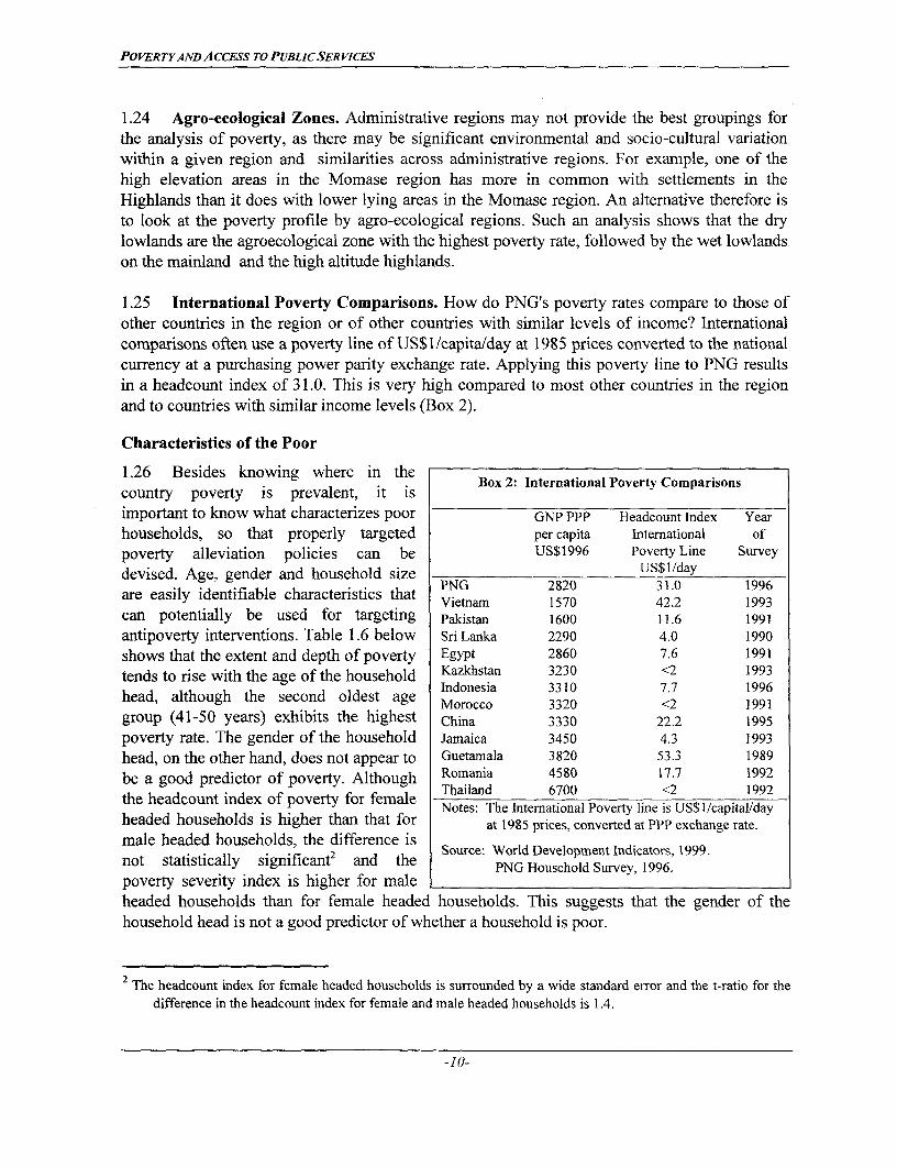
1.25 International Poverty Comparisons. How do PNG's poverty rates compare to those ofother countries in the region or of other countries with similar levels of income? Internationalcomparisons often use a poverty line of US$1/capitalday at 1985 prices converted to the nationalcurrency at a purchasing power parity exchange rate. Applying this poverty line to PNG resultsin a headcount index of 31.0. This is very high compared to most other countries in the regionand to countries with similar income levels (Box 2).
Characteristics of the Poor
1.26 Besides knowing where in thecountry overty i prevalet, it isBox 2: International Poverty Comparisonscountry poverty is prevalent, it iS
important to know what characterizes poor GNP PPP Headcount Index Yearhouseholds, so that properly targeted per capita International ofpoverty alleviation policies can be US$1996 Poverty Line Survey
devised. Age, gender and household size US$1/dayare easily identifiable characteristics that PNG 2820 31.0 1996
Vietnam 1570 42.2 1993can potentially be used for targeting Pakistan 1600 11.6 1991
antipoverty interventions. Table 1.6 below SriLanka 2290 4.0 1990
shows that the extent and depth of poverty Egypt 2860 7.6 1991tends to rise with the age of the household Kazkhstan 3230 <2 1993
Indonesia 3310 7.7 1996head, although the second oldest age Morocco 3320 <2 1991
group (41-50 years) exhibits the highest China 3330 22.2 1995
poverty rate. The gender of the household Jamaica 3450 4.3 1993head, on the other hand, does not appear to Guetamala 3820 53.3 1989be a good predictor of poverty. Although Romania 4580 17.7 1992the headcount index of poverty for female Thailand 6700 <2 1992
Notes: The International Poverty line is US$ 1/capitalldayheaded households is higher than that for at 1985 prices, converted at PPP exchange rate.
male headed households, the difference is S2 ~~~~Source: World Development Indicators, 1999.
not statistically significant2 and the PNG Household Survey, 1996.
poverty severity index is higher for male Iheaded households than for female headed households. This suggests that the gender of thehousehold head is not a good predictor of whether a household is poor.
2 The headcount index for female headed households is surrounded by a wide standard error and the t-ratio for thedifference in the headcount index for female and male headed households is 1.4.
-10-

POVERTYAND ACCESS TO PUBLIC SER VICES
Figure 1.3: Headcount Index and Contribution to Poverty by Agro-ecological Region(based on foot-poverty line)
40 wet island lowlands highlands
30 _dry lowlands25 - E high altitude O Headcount Index25 - wet mainland highlands I * Contribution to National Poverty20 -lowlands
10 - _ _ | small urban10 5 major urban0 _
Source: PNG Household Survey 1996
1.27 Poverty increases with household size and with the number of children per householdwhen no allowance is made for economies of size in household consumption (Table 1.6).However, these results must be interpreted with caution, because larger households typicallyappear to be poorer when no allowance for household size economies is made. Economies of sizein household consumption allow the cost per person of reaching a certain standard of living tofall as household size rises. For example, a household with ten people may not need to spend tentimes as much as a single-person household to enjoy the same standard of living. However, thereis no fully satisfactory method of determining the proper correction factor for size economies inpractice. Annex I carries out some sensitivity analysis, by setting the correction factor to variouslevels and finds that indeed the relationship between household size and poverty becomes lessprominent once corrections are made for household size economies.
1.28 The relationship between poverty and education is critical because education is the majorhuman capital investment that individuals face. As Table 1.7 demonstrates, educationalattainment of a household's head is also a good predictor for poverty. Over half of all poor peoplelive in a household whose head has never attended school, although they are only 38 percent oftotal population. The poverty rate among this group is 51 percent, well above the nationalaverage. The poverty rate drops by 10 percentage points for households where the head attendedschool but did not graduate from community school and poverty continues to fall with risingeducational attainments of household heads. This is not surprising, as higher education levelsprovide better opportunities to diversify income and engage in non-traditional income generation.It also points to the importance of providing the poor with increased access to education as amechanism of poverty alleviation. (see Chapter 2).
-11-

POVERTYANDACCESS TO PUBLICSERVICES
Table 1.6: Poverty by Household Size, Age and Gender of Household Head
Headcount IndexI Poverty Severity Index1 Population ShareIndex Contribution to Index Contribution to (%/-)
total poverty (%/o) total poverty (%)
Age of Household Head0-30years 33.1 17.4 5.4 19.0 19.731-40 years 32.2 30.4 4.6 28.9 35.441-50 years 46.0 27.7 7.0 28.3 22.651+ years 41.4 24.5 6.0 23.7 22.2
Gender of Household HeadMale 36.8 91.8 5.6 94.5 93.6Female 48.1 8.2 4.7 5.5 6.4
Household Size2
1-2 persons 17.2 1.3 1.6 0.9 2.93-4 persons 27.4 12.5 4.6 14.1 17.15-6 persons 32.2 20.5 5.3 22.6 23.97-8 persons 40.1 25.6 5.9 25.5 24.09-10 persons 45.7 19.8 6.4 18.6 16.3> 10 persons 48.1 20.2 6.5 18.3 15.7
Number of Children inHousehold 2
No children 22.7 4.1 3.4 4.2 6.81-2 children 29.8 24.4 4.5 24.9 30.73-4 children 40.4 40.2 6.2 41.6 37.45-6 children 40.6 21.0 5.6 19.3 19.5> 6 children 67.1 10.3 9.8 10.0 5.7
Notes: 1. Based on Upper Poverty Line2. Poverty measures are for per capita household consumption, without allowance for size economies.
These results, therefore, must be interpreted with caution. See Annex I for details.
Source: PNG Household Survey 1996
Table 1.7: Poverty by Educational Attainment of Household Head
Headcount Poverty Severity PopulationShare
Index Contribution Index Contribution to (%)to total total poverty
poverty (%) (/)
Education of Household HeadNo schooling 51.0 51.7 8.0 54.2 38.0< grade 6 40.6 22.7 6.6 24.7 21.0Community school (gr. 6) 30.9 13.9 4.1 12.3 16.9High school (gr. 7-12) 16.0 4.6 1.8 3.5 10.8Vocational ed. 23.9 7.1 2.7 5.3 11.1University ed. 0.0 0.0 0.0 0.0 2.1
Source: PNG Household Survey 1996
-12-
POVERTYANDACCESS TO PUBLIC SER VICES
1.29 Poverty and Sources of Income. The ability to earn cash is an important determinant ofwhether a person is poor or not. Even in Papua New Guinea, where much of householdconsumption is self-produced, cash incomes are needed for essential non-food items such asschool fees, kerosene, and garden tools. Cash can also improve the quality of the diet and provideinsurance for periods of agricultural stress. Thus it is important to examine the relationshipbetween poverty and the income earning activities of working-age household members.
1.30 People living in households where the household head derives income mainly from minornon-agricultural activities such as hunting, fishing and gathering have the highest poverty rate, at57 percent (Table 1.8). The next highest poverty rate is for people in households where the headdoes not have any cash earning activities. The poverty rate is lower, but still above average, forhouseholds where the head's main source of income is from either domestic agriculture (betelnut,food crops, livestock) or export tree crop agriculture (mainly coffee, cocoa, copra, oil palm). Acloser look at the main components of domestic agriculture - betelnut, food crops, and livestock- suggest that the three income categories bring similar risks of poverty, although there is a smalldisadvantage when the head earns most of their income from livestock.
1.31 There are wide differences in the risk of poverty according to which export tree cropprovides income for the household head. The risk of being poor is greatest for households whosehead earns money from growing cocoa. People living in households whose head grows coffeealso have above average poverty rates, and this group constitutes over one-quarter of thecountry's poor. The lowest poverty rate for tree crop producers in 1996 was for oil palm growers.These variations in poverty rates amongst tree crop producing households partly reflectinternational market conditions, with 1996 being a good year for oil palm prices after several lowpriced years earlier in the decade3.
1.32 The lowest poverty rates are for households whose head has a wage job or gets incomefrom a formal business. There is a premium to being employed in the public sector, in terms of alower poverty rate. The incidence, depth, and severity of poverty is lower for public sector wageworkers than for private sector wage workers. A household whose head works in the privatesector has a two-thirds greater likelihood of being below the upper poverty line, compared with ahousehold headed by a public sector worker.
1.33 In terms of the contribution to national poverty, almost one-half (43 percent) of the poorlive in households where tree crop agriculture provides the main source of income for the
3 The sample size of the survey prevents a meaningful comparison of poverty rates of different types of tree cropproducers between regions. While it is important to note that poverty is widespread among export tree cropproducers across the country, it must be kept in mind that characteristics and conditions of producers of eventhe same tree crop (say coffee) can vary widely between regions and even within a given region. This meansthat any meaningful intervention to help raise living standards of export tree crop producers would have to betailored to local conditions. The same applies to other categories of agricultural producers with high povertyrates.
-13-

POVERTYAND ACCESS TO PUBLIC SER VICES
household head. A further 19 percent live in households where the head gets most of theirincome from agricultural sales for the local market. Thus, almost two-thirds of the poor are foundin households where the head relies upon agriculture for the main source of income, even thoughthis group is only 53 percent of the population. The next major contributor to poverty ishouseholds where the head does not earn any cash income and is thus mainly engaged insubsistence agriculture. (17 percent). Although people in hunter-gatherer households have thehighest poverty rate, they are only a small group of the population (5.1 percent), so theycomprise just eight percent of the total poor. Only 14 percent of the poor live in householdswhere the head has a wage job or formal business, even though this group comprises 29 percentof the population.
Table 1.8: Incidence and Severity of Poverty by Main Income Source of Household Head
Headcount Index Poverty Severity Index
Index Contribution to total Index Contribution to % of
poverty (%/o) total poverty (%ND) population
No income source (1) 46.9 16.6 9.5 22.6 13.3
Fishing, hunting, gathering 57.3 7.9 7.5 6.9 5.1
Domestic Agriculture 42.7 19.0 5.5 16.6 16.7
Betelnut 38.1 5.4 5.0 4.7 5.3
Food Crops 43.2 6.8 5.2 5.5 5.9
Livestock 46.5 6.8 6.4 6.3 5.5
Cash Crops 44.0 42.5 6.6 42.8 36.3
Coffee 41.5 26.1 6.8 28.8 23.6
Cocoa 56.6 7.9 8.0 7.5 5.2
Copra 50.2 5.8 6.3 4.9 4.3
Oil Palm 32.3 2.6 2.1 1.1 3.0
Running a business 24.6 4.2 2.7 3.1 6.4
Wagejob 16.6 9.8 2.0 8.1 22.2
Public 13.5 4.4 1.6 3.6 12.2
Private 20.3 5.4 2.5 4.5 10.0
Notes: (1) No income source means that the household head does not earn any cash income, but the household
may still obtain cash income from other household members.
(2) Poverty measures at upper
poverty line
Source: PNG Household Survey 1996. Box 3: Summary Profile of Poor
1.34 The main income source of Poor Non-Poor
the household head is an importantvariable for classifying households. averageyearsofschooling of household head 2,4 5,0
However, it is also worthwhile % of household head completed community school 24,3 49,5
studying the relationship between % of household head completed secondary/technical school 7,9 23,6% literate 36,3 64,1poverty and other (i.e., secondary) % living in rural areas 95,6 82,1
income sources, whether these be % with main income from agriculture 62,2 52,7% female headed households 10,4 6,7
from alternative activities of the average floor area per capita 6,4 9,8
household head or from the earnings % access to piped water 3,3 15,0average real expenditure/adult equivalent 277,0 1287,0
Source: PNG Household Survey 1996
-14-

POVERTYAND ACCESS TO PUBLICSERVICES
of other household members. Almost one-third of all working-age adults do not participate inany cash earning activities. The most common primary income sources for individuals are:coffee, which gives primary employment for 19 percent of the working-age population, foodcrops (14 percent; of which one-third is solely sweet potato), betelnut (7 percent), and privatesector wage jobs (6 percent).
Box 4: Summary Profile of Poor Households by Region
Poor Non-Poor Poor Non-Poor Poor Non-Poor Poor Non-Poor Poor Non-Poor Poor Non-poorNCD NCD Papuan Papuan Highlands Highlands Momase Momase NGI NGI
Household Size 6.59 5.44 10.1 6.2 6.7 5.7 6.5 5.7 6.4 5.0 6.6 4.9
average years of 2.41 5.02 4.7 10.9 2.6 6.4 1.4 3.4 2.7 5.3 4.8 5.0schooling of householdhead% ofhouseholdhead 24.3 49.5 41 92 27 65 14 36 26 51 50 51completed communityschool% of household head 7.9 23.6 19 73 n.a. 34 5 13 10 24 21 20completedsecondary/technicalschool% literate 36.3 64.1 77 97 38 72 20 45 43 73 67 80
%living in rural areas 95.6 82.1 0 0 100 89 100 97 96 71 94 91
% with main income 62.2 52.7 5 4 58 43 59 58 71 55 60 64from agriculture%femaleheaded 10.4 6.7 4 13 2 1 5 6 17 6 21 15householdsaverage floorareaper 6.4 9.8 4.5 15.1 6.5 9.1 5.3 7.6 7.7 11.7 6.0 11.3capita (m2)% access to piped water 3.3 15.0 86 96 0 5 2 7 2 22 0 0
average real 277 1287 320 1816 248 1126 287 1158 275 1630 269 863expenditure/adultequivalent (kina)
Source: PNG Household Survey, 1996.
1.35 Which primary income sources are important for poor people? Working-age adults in thehouseholds covered by the household survey were classified as poor if their household'sconsumption level was below the upper poverty line (i.e., intra-household equality is assumed).The highest poverty rates were for people engaged in minor activities (hunting and gathering,miscellaneous livestock raising, spices and vanilla, and handicrafts and artifacts). Amongst themore important economic activities, the highest poverty rates were for people primarily earningfrom cocoa (45 percent), other food crops (43 percent), and those with no cash earning activities(39 percent). The lowest poverty rates were for people with formal businesses and wage jobs.Overall, the poverty profile by income source thus varies little whether the income source of thehousehold head or the income source of all working age adults is considered.
-15-

POVERTYAND ACCESS To PUBLIC SER VICES
Table 1.9: Poverty And Income Sources For Working-Age Adults
Main Income Source All Earning Activities
Income earning activity Participation Poverty Participation Female % of
Rate Rate Ratea participants
Coffee 18.5 38.5 22.3 43.0
Cocoa 4.3 45.2 11.2 45.5
Copra 3.7 36.4 6.1 49.4
Betelnut 6.5 29.7 20.2 68.1
Sweet potato 4.2 32.4 19.6 87.4Other food 9.8 42.6 26.6 82.6
Oil palm 1.6 25.8 2.4 27.0
Pyrethrum, spices, vanilla 0.1 46.2 1.7 81.2
Chickens 0.9 9.5 5.3 45.3
Pigs 2.4 35.9 9.6 36.3
Cattle and other livestock 0.1 48.0 0.3 33.3
Catching and selling fish 1.4 34.7 5.7 51.8
Hunting, selling bush animals 0.6 69.2 4.9 40.1Gathering, selling firewood 0.3 70.1 1.0 49.4Making, selling artifacts 1.3 42.3 5.0 83.9Owning, running a store 0.8 10.2 2.4 49.6
P.M.V. business 0.2 5.1 0.5 22.1
Running another business 1.6 24.0 3.4 39.2Wage job-public sector 4.4 12.9 5.0 17.4Wage job - agricultural sector 0.6 13.4 0.8 16.8
Wage job - other private sector 5.6 18.7 6.9 16.3
No cash earning activities 31.0 38.8 31.0 48.4
a Sums to more than 100 because some people earn income from multiple activities.Source: PNG Household Survey 1996
1.36 The conclusion which results from this poverty profile is that the vast majority of poorpeople in PNG live in rural areas. Many of them do not earn any cash income and thus derivetheir livelihood almost entirely from subsistence agriculture. Of those who earn cash income,poverty is highest among those engaged in small scale tree crop production, domestic agricultureand hunting - gathering. Poverty is significantly more widespread among households whosehead has not attended school. Over 40 percent of all poor households in PNG derive their mainincome from the production of export tree crops. Poverty is highest in the MomaselNorth Coastregion, but in absolute terms, the highest number of poor households live in the Highlandsregion. Together these two regions account for three quarters of PNG's poor.
-16-

POVERTYAND ACCESS To PUBLIC SER VICES
2. POVERTY AND ACCESS TO PUBLIC SERVICES
A. INTRODUCTION
2.1 Although consumption-based measures of poverty provide a good indication of thedistribution of living standards, they do not fully take into account other dimensions of welfare.Access to publicly provided basic services has a direct impact on the welfare of the population.Unequal access to health, education, transport facilities and utilities can further accentuate theeffects of an unequal income distribution.
2.2 Data from the household survey show that lower expenditure groups in PNG faresignificantly worse than the upper groups across a wide range of social indicators (Table 2.1).Because most of these indicators are substantially influenced by access to basic services such aseducation, health care, rural infrastructure and utilities, the distribution of access to such servicesmerits closer analysis.
Table 2.1: Distribution Of Social Indicators Across Expenditure Groups
Poorest Second Third Richest PNGQuartile Quartile Quartile Quartile
Literacy% women aged 15+ 31 38 44 57 43% of men aged 15+ 48 54 61 77 61Never attended school% of women aged 15+ 60 54 47 37 49% of menaged 15+ 40 38 29 20 31
Stunting 52 44 42 34 43% of children 0-5 yearsPiped water 4 6 11 27 12% of householdsFlush toilet 0 3 5 21 7% of householdsElectricity 2 3 13 31 12% of households
Source: PNG Household Survey 1996
2.3 There is a clear positive correlation between the level of consumption and a person'ssatisfaction with his or her family's access to public services, such as health care, education andtransport facilities (Table 2.2). This suggests that the upper income groups benefit from betteraccess to basic public services than the poor. However, it is striking that PNG's populationoverall shows a very low level of satisfaction with the provision of basic social services. Overhalf the population consider that their children do not get appropriate access to schooling, almost60 percent consider their access to health care unsatisfactory and two thirds of the populationexpress dissatisfaction with their access to public transportation. The level of satisfaction with
-17-

POVERTYAND ACCESS TO PUBLIC SER VICES
access to public services varies significantly across regions and is generally lowest in the regionswhere poverty is most severe.
Table 2.2: Perceptions About Adequacy of Public Services
% of population who believe that they have inadequate access to servicescompared to their family's needs
Health Care Children's Public Transportschooling
ConsumptionQuartilePoorest 64 59 75Second 63 55 78Third 60 50 66Richest 50 44 48
RegionNCD 36 28 25Papuan/South Coast 50 45 81Highlands 63 61 67Momase/North Coast 65 57 68New Guinea Islands 46 30 62
PNG 59 52 67
Source: PNG Household Survey 1996
B. HEALTH AND NUTRITION
Health
2.4 Health Indicators. Although PNG has a relatively well developed health careinfrastructure, the health and nutritional status of its population compares unfavorably to that ofother countries in the region and has stagnated over the past decade (Table 2.3).
2.5 Deteriorating status of health infrastructure. The low health standards, despite arelatively well developed health care infrastructure, point to unsatisfactory performance andsubstantial inefficiencies in PNG's health care system. The physical status of the infrastructurehas deteriorated substantially over the past two decades. As a result, a vast majority of facilitiesare now in unsatisfactory condition and provide services poorly. According to the 1996Demographic and Health Survey, only 39 percent of health facilities are in satisfactory conditionand only about 70 percent of rural aid posts are operating. There are also marked regionalvariations in the availability, operational condition and performance of health care facilities. Forexample, availability of aid posts or health centers ranges from a high of 267 facilities per
-18-
POVERTYAND ACCESS TO PUBLIC SERVICES
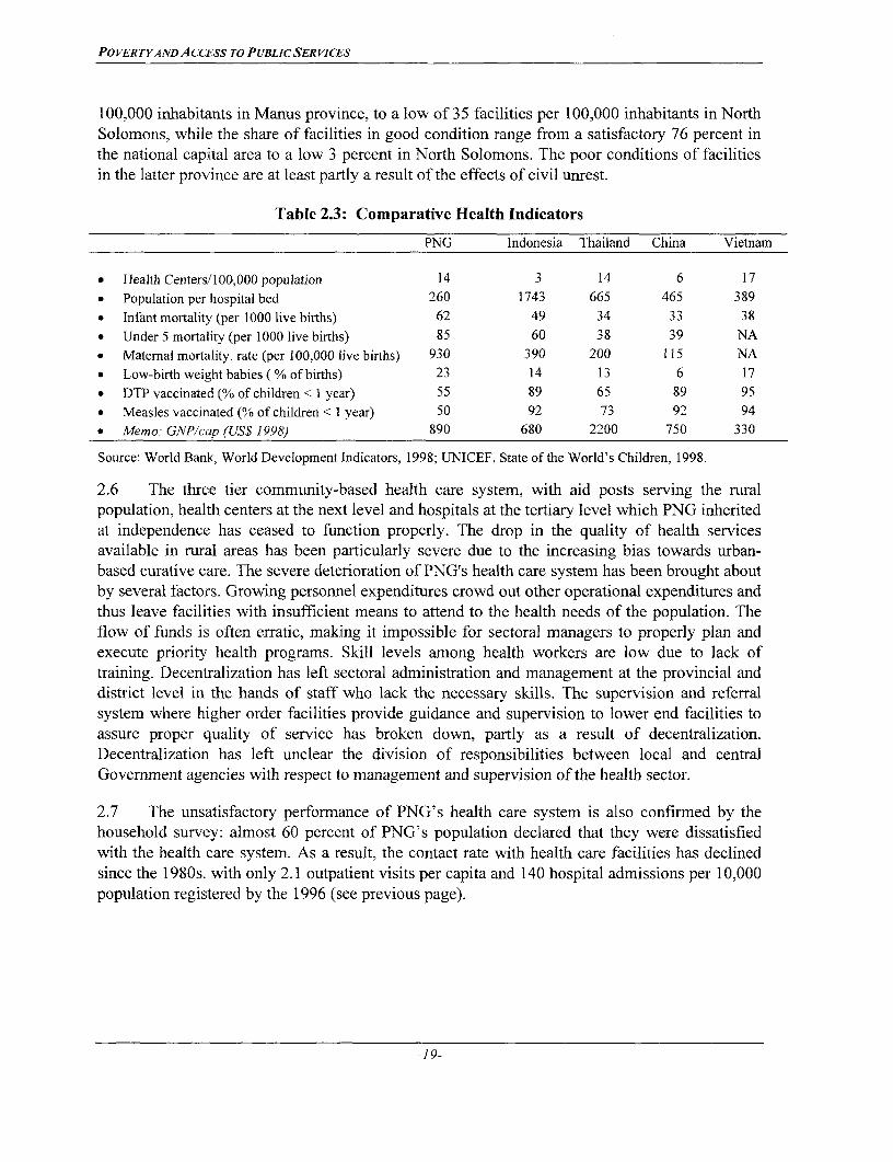
100,000 inhabitants in Manus province, to a low of 35 facilities per 100,000 inhabitants in NorthSolomons, while the share of facilities in good condition range from a satisfactory 76 percent inthe national capital area to a low 3 percent in North Solomons. The poor conditions of facilitiesin the latter province are at least partly a result of the effects of civil unrest.
Table 2.3: Comparative Health Indicators
PNG Indonesia Thailand China Vietnam
* Health Centers/lOO,000 population 14 3 14 6 17* Population per hospital bed 260 1743 665 465 389* Infant mortality (per 1000 live births) 62 49 34 33 38* Under 5 mortality (per 1000 live births) 85 60 38 39 NA* Matemal mortality. rate (per 100,000 live births) 930 390 200 115 NA* Low-birth weight babies ( % of births) 23 14 13 6 17* DTP vaccinated (% of children < I year) 55 89 65 89 95* Measles vaccinated (% of children < I year) 50 92 73 92 94* Memo: GNP/cap (US$ 1998) 890 680 2200 750 330
Source: World Bank, World Development Indicators, 1998; UNICEF, State of the World's Children, 1998.
2.6 The three tier community-based health care system, with aid posts serving the ruralpopulation, health centers at the next level and hospitals at the tertiary level which PNG inheritedat independence has ceased to function properly. The drop in the quality of health servicesavailable in rural areas has been particularly severe due to the increasing bias towards urban-based curative care. The severe deterioration of PNG's health care system has been brought aboutby several factors. Growing personnel expenditures crowd out other operational expenditures andthus leave facilities with insufficient means to attend to the health needs of the population. Theflow of funds is often erratic, making it impossible for sectoral managers to properly plan andexecute priority health programs. Skill levels among health workers are low due to lack oftraining. Decentralization has left sectoral administration and management at the provincial anddistrict level in the hands of staff who lack the necessary skills. The supervision and referralsystem where higher order facilities provide guidance and supervision to lower end facilities toassure proper quality of service has broken down, partly as a result of decentralization.Decentralization has left unclear the division of responsibilities between local and centralGovernment agencies with respect to management and supervision of the health sector.
2.7 The unsatisfactory performance of PNG's health care system is also confirmed by thehousehold survey: almost 60 percent of PNG's population declared that they were dissatisfiedwith the health care system. As a result, the contact rate with health care facilities has declinedsince the 1980s. with only 2.1 outpatient visits per capita and 140 hospital admissions per 10,000population registered by the 1996 (see previous page).
-19-
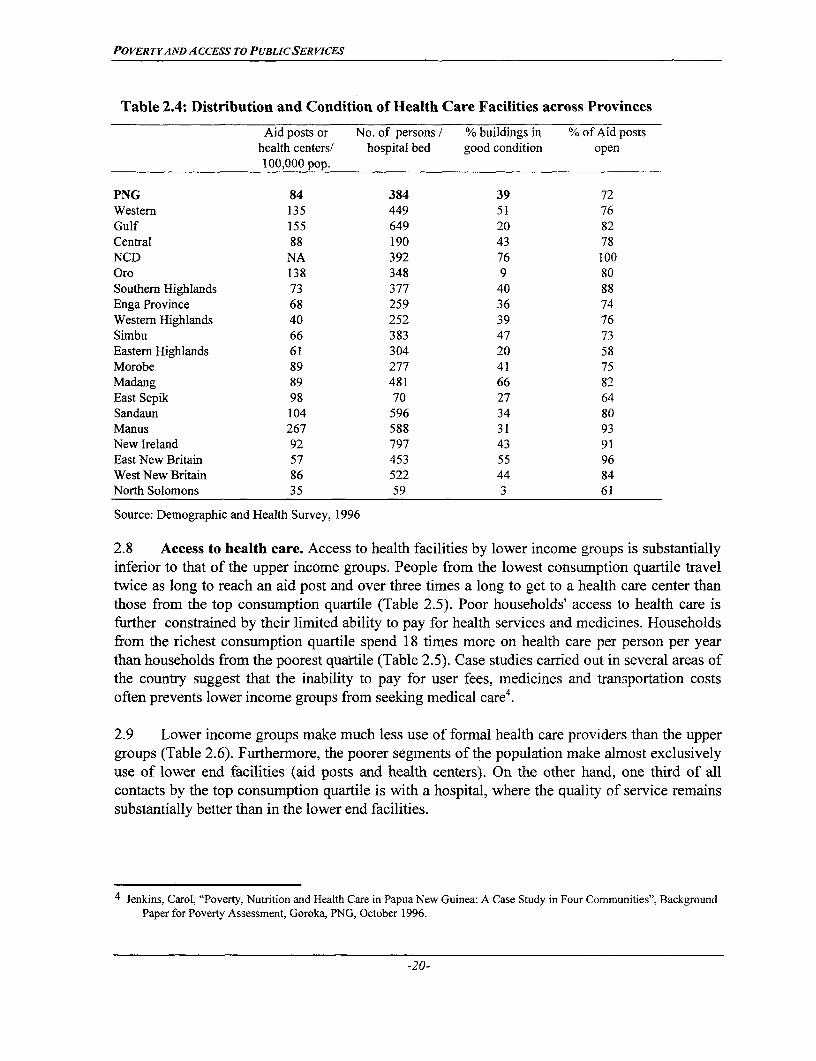
POVERTYAND ACCESS TO PUBLIC SER VICES
Table 2.4: Distribution and Condition of Health Care Facilities across Provinces
Aid posts or No. of persons / % buildings in % of Aid posts
health centers/ hospital bed good condition open
1 00,000 pop.
PNG 84 384 39 72
Western 135 449 51 76
Gulf 155 649 20 82
Central 88 190 43 78
NCD NA 392 76 100
Oro 138 348 9 80
Southem Highlands 73 377 40 88
Enga Province 68 259 36 74
Western Highlands 40 252 39 76
Sirnbu 66 383 47 73
Eastern Highlands 61 304 20 58
Morobe 89 277 41 75
Madang 89 481 66 82
East Sepik 98 70 27 64
Sandaun 104 596 34 80
Manus 267 588 31 93
New Ireland 92 797 43 91
East New Britain 57 453 55 96
West New Britain 86 522 44 84
North Solomons 35 59 3 61
Source: Demographic and Health Survey, 1996
2.8 Access to health care. Access to health facilities by lower income groups is substantiallyinferior to that of the upper income groups. People from the lowest consumption quartile traveltwice as long to reach an aid post and over three times a long to get to a health care center thanthose from the top consumption quartile (Table 2.5). Poor households' access to health care isfurther constrained by their limited ability to pay for health services and medicines. Householdsfrom the richest consumption quartile spend 18 times more on health care per person per yearthan households from the poorest quartile (Table 2.5). Case studies carried out in several areas ofthe country suggest that the inability to pay for user fees, medicines and transportation costsoften prevents lower income groups from seeking medical care4.
2.9 Lower income groups make much less use of formal health care providers than the uppergroups (Table 2.6). Furthermore, the poorer segments of the population make almost exclusivelyuse of lower end facilities (aid posts and health centers). On the other hand, one third of allcontacts by the top consumption quartile is with a hospital, where the quality of service remainssubstantially better than in the lower end facilities.
4 Jenkins, Carol, "Poverty, Nutrition and Health Care in Papua New Guinea: A Case Study in Four Communities", BackgroundPaper for Poverty Assessment, Goroka, PNG, October 1996.
-20-
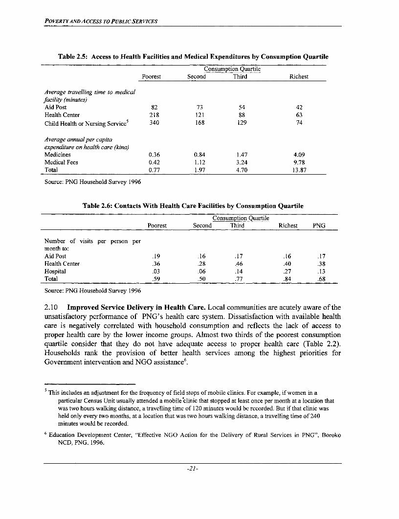
POVERTYANDACCESS TO PUBLICSERVICES
Table 2.5: Access to Health Facilities and Medical Expenditures by Consumption Quartile
Consumption QuartilePoorest Second Third Richest
Average travelling time to medicalfacility (minutes)Aid Post 82 73 54 42Health Center 218 121 88 63Child Health or Nursing Service5 340 168 129 74
Average annual per capitaexpenditure on health care (kina)Medicines 0.36 0.84 1.47 4.09Medical Fees 0.42 1.12 3.24 9.78Total 0.77 1.97 4.70 13.87
Source: PNG Household Survey 1996
Table 2.6: Contacts With Health Care Facilities by Consumption Quartile
Consumption QuartilePoorest Second Third Richest PNG
Number of visits per person permonth to:Aid Post .19 .16 .17 .16 .17Health Center .36 .28 .46 .40 .38Hospital .03 .06 .14 .27 .13Total .59 .50 .77 .84 .68
Source: PNG Household Survey 1996
2.10 Improved Service Delivery in Health Care. Local communities are acutely aware of theunsatisfactory performance of PNG's health care system. Dissatisfaction with available healthcare is negatively correlated with household consumption and reflects the lack of access toproper health care by the lower income groups. Almost two thirds of the poorest consumptionquartile consider that they do not have adequate access to proper health care (Table 2.2).Households rank the provision of better health services among the highest priorities forGovernment intervention and NGO assistance6 .
5This includes an adjustment for the frequency of field stops of mobile clinics. For example, if women in aparticular Census Unit usually attended a mobile 'clinic that stopped at least once per month at a location thatwas two hours walking distance, a travelling time of 120 minutes would be recorded. But if that clinic washeld only every two months, at a location that was two hours walking distance, a travelling time of 240minutes would be recorded.
6 Education Development Center, "Effective NGO Action for the Delivery of Rural Services in PNG", BorokoNCD, PNG, 1996.
-21-

POVERTYAND ACCESS TO PUBLIC SER VICES
2.11 Health reform is critical to raise the population's health standards and to improve thelower income groups' access to proper health care. Devolution has shifted the responsibility toprovide health care to provincial and district governments. However, local governments largelylack the institutional capacity to appropriately manage the health care system and assure properservice delivery7 . Therefore, the responsibilities of government agencies involved in health careneed to be carefully reviewed. Responsibilities must be clearly designated and the institutions incharge must have acquired the necessary institutional capacity to carry out their job properly.NGOs and churches constitute an important partner in the area of local service provision. Thecollaboration and coordination between the public sector, the private sector and the NGO sectorin this area must be increased.
2.12 There is also an important need to review the allocation of public sector resources in thehealth sector. This will show whether expenditure priorities are in line with the health needs ofPNG's population. Many countries with poor or falling health performance indicators have foundthat a reallocation of public expenditures in line with the population's health needs couldsubstantially help increase the sector's performance and improve the lower income groups'access to health care. Such expenditure reallocations generally shift resources away fromexpensive tertiary care which tends to excessively benefit the upper income groups in urbanareas, towards basic primary care provided at the local level. Lack of detailed expenditure dataon health prevented such an analysis in this report, but it should be made a high priority so that itcan help guide decision making with respect to health care reform in PNG.
Water and Sanitation
2.13 Availability of clean water and adequate sanitation has an important bearing on thepopulation's health status. The household survey showed that access to safe drinking water is animportant issue across PNG, with over 60 percent of the population relying on rivers, lakes,creeks and similar unprotected sources for drinking water (Table 2.7). The poor are particularlyat risk from unsafe water: over 80 percent of the lowest consumption quartile get their drinkingwater from unprotected sources. This ratio is almost twice as high as that for the richest 25percent of the population. Not surprisingly, households ranked improvements in access to safewater as one of the highest priorities for Government intervention during the household survey.Given the importance of protected water supply to the population's health and welfare, theGovernment should make provision of safe water a high priority item in the area of public health.
Poverty and Malnutrition
2.14 Adequate nutrition is not only important for an individual's physical well-being, it is alsocrucial for a person's long term development. Chronic malnutrition, particularly during earlychildhood, can have a negative impact on a child's mental development, thus reducing his or herchances for future income earning opportunities.
7 See for example, D. Campos-Outcall, K. Kewa and J. Thomason, "Decentralization of Health Services in WesternHighlands Province, PNG", in Social Science and Medicine, Vol 40, No. 8, pp. 1091-1098, 1995.
-22-
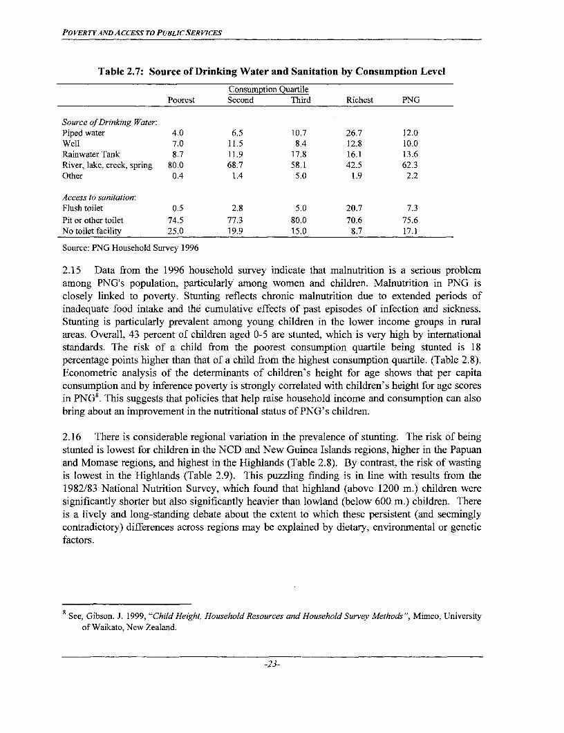
POVERTYAND ACCESS To PUBLIC SER VICES
Table 2.7: Source of Drinking Water and Sanitation by Consumption Level
Consumption QuartilePoorest Second Third Richest PNG
Source of Drinking Water:Piped water 4.0 6.5 10.7 26.7 12.0Well 7.0 11.5 8.4 12.8 10.0RainwaterTank 8.7 11.9 17.8 16.1 13.6River, lake, creek, spring 80.0 68.7 58.1 42.5 62.3Other 0.4 1.4 5.0 1.9 2.2
Access to sanitation:Flush toilet 0.5 2.8 5.0 20.7 7.3Pit or other toilet 74.5 77.3 80.0 70.6 75.6No toilet facility 25.0 19.9 15.0 8.7 17.1
Source: PNG Household Survey 1996
2.15 Data from the 1996 household survey indicate that malnutrition is a serious problemamong PNG's population, particularly among women and children. Malnutrition in PNG isclosely linked to poverty. Stunting reflects chronic malnutrition due to extended periods ofinadequate food intake and the cumulative effects of past episodes of infection and sickness.Stunting is particularly prevalent among young children in the lower income groups in ruralareas. Overall, 43 percent of children aged 0-5 are stunted, which is very high by internationalstandards. The risk of a child from the poorest consumption quartile being stunted is 18percentage points higher than that of a child from the highest consumption quartile. (Table 2.8).Econometric analysis of the determinants of children's height for age shows that per capitaconsumption and by inference poverty is strongly correlated with children's height for age scoresin PNG8. This suggests that policies that help raise household income and consumption can alsobring about an improvement in the nutritional status of PNG's children.
2.16 There is considerable regional variation in the prevalence of stunting. The risk of beingstunted is lowest for children in the NCD and New Guinea Islands regions, higher in the Papuanand Momase regions, and highest in the Highlands (Table 2.8). By contrast, the risk of wastingis lowest in the Highlands (Table 2.9). This puzzling finding is in line with results from the1982/83 National Nutrition Survey, which found that highland (above 1200 m.) children weresignificantly shorter but also significantly heavier than lowland (below 600 m.) children. Thereis a lively and long-standing debate about the extent to which these persistent (and seeminglycontradictory) differences across regions may be explained by dietary, environmental or geneticfactors.
8 See, Gibson. J. 1999, "Child Height, Household Resources and Household Survey Methods ", Mimeo, Universityof Waikato, New Zealand.
-23-
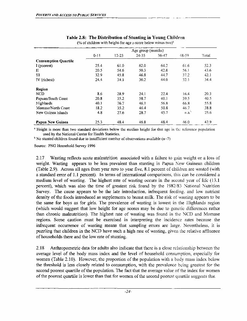
POVERTYAND ACCESS TO PUBLIC SER viCES
Table 2.8: The Distribution of Stunting in Young Children(% of children with height-for-age z-score below minus two)a
Age group (months)0-11 12-23 24-35 36-47 48-59 Total
Consumption QuartileI (poorest) 25.4 61.0 62.0 64.2 61.6 52.3II 20.5 54.6 50.3 42.8 56.1 43.6III 32.9 45.8 46.8 44.7 37.2 42.1IV (richest) 24.4 34.1 30.2 44.0 32.1 34.4
RegionNCD 8.6 28.9 24.1 22.4 16.4 20.3Papuan/South Coast 20.8 35.2 58.7 40.1 39.5 40.5Highlands 40.1 76.7 46.1 56.8 66.8 55.8Momase/North Coast 18.2 35.2 46.4 50.8 46.7 38.8New Guinea Islands 4.8 27.6 28.7 45.7 n.a.b 25.6
Papua New Guinea 25.3 48.4 46.8 48.4 46.0 42.9
a Height is more than two standard deviations below the median height for that age in the reference populationused by the National Center for Health Statistics.
bNo stunted children found due to insufficient number of observations available (n=7)
Source: PNG Household Survey 1996
2.17 Wasting reflects acute malnutrition associated with a failure to gain weight or a loss ofweight. Wasting appears to be less prevalent than stunting in Papua New Guinean children(Table 2.9). Across all ages from year zero to year five, 8.1 percent of children are wasted (witha standard error of 1.1 percent). In terms of international comparisons, this can be considered amedium level of wasting. The highest rate of wasting occurs in the second year of life (13.1percent), which was also the time of greatest risk found by the 1982/83 National NutritionSurvey. The cause appears to be the late introduction, infrequent feeding, and low nutrientdensity of the foods introduced as supplements to breast milk. The risk of wasting appears to bethe same for boys as for girls. The prevalence of wasting is lowest in the Highlands region(which would suggest that low height for age scores may be due to genetic differences ratherthan chronic malnutrition). The highest rate of wasting was found in the NCD and Momaseregions. Some caution must be exercised in interpreting the incidence rates because theinfrequent occurrence of wasting means that sampling errors are large. Nevertheless, it ispuzzling that children in the NCD have such a high rate of wasting, given the relative affluenceof households there and the low rate of stunting.
2.18 Anthropometric data for adults also indicate that there is a close relationship between theaverage level of the body mass index and the level of household consumption, especially forwomen (Table 2.10). However, the proportion of the population with a body mass index belowthe threshold is less closely related to consumption, with the prevalence being greatest for thesecond poorest quartile of the population. The fact that the average value of the index for womenof the poorest quartile is lower than that for women of the second poorest quartile suggests that
-24-

POVERTYAND ACCESS To PUBLIC SER VICES
some women in the poorest quartile must have a very low body mass index. Overall, the risk ofchronic energy deficiency as measured by a low body mass index is three times higher forwomen than for men.
Table 2.9: The Distribution of Wasting in Young Children(% of children with weight-for-height z-score below minus two)a
Age group (months)
0-11 12-23 24-35 36-47 48-59 Total
Consumption QuartileI (poorest) 19.8 13.9 0.0 6.1 6.8 9.8II 12.1 22.0 4.1 6.2 11.7 10.4
III 8.7 12.1 1.3 2.7 5.6 6.1IV (richest) 6.6 4.7 4.3 11.0 1.3 5.9
Region
NCD 13.3 28.9 20.1 9.4 9.4 17.5
Papuan/South Coast 16.2 6.6 0.0 14.8 0.0 7.9Highlands 3.9 4.8 3.0 1.9 4.9 3.5Momase/North Coast 21.0 24.0 2.5 4.0 13.3 12.2New Guinea Islands 6.2 10.0 0.0 10.0 0.0 6.6
Papua New Guinea 12.0 13.1 2.7 6.5 6.0 8.1
Weight is more than two standard deviations below the median weight for that height in the referencepopulation used by the National Center for Health Statistics.
Source: PNG Household Survey 1996
2.19 An analysis of the determinants of child growth in PNG suggests that a mother's level ofeducation and her own height have a significant impact on the long term nutritional status of herchildren (Annex IV). The higher the level of a mother's education, the less likely her children areto suffer from chronic malnutrition. Controlling for parental height, and household economicresources, the analysis indicates that each additional year of schooling of the mother results in a 2percent decrease in the likelihood of her child being stunted. This effect is four times higher thanthat of an additional year of schooling of the father9 .
2.20 The marked effects of a mother's height and education on her children's stuntingprobabilities indicate that there is a long-run, intergenerational effect of women's education onchild health. Educating the current generation of girls will reduce the risk that their own childrenare stunted. Those children are likely to become taller adults which will then reduce the risk ofthe next generation of children being stunted. This suggests that there is a role for public action
9The associations between maternal education and stature and children's stunting depicted by the PNG Household
Survey are consistent with finding of earlier localized studies from various parts of PNG. See, for example,Harvey P.W.J et. al. (1984); Groos. A. and R.L. Hide (1989); Gibson, J. (1996).
-25-

POVERTYANDACCESS TO PUBLICSERVICES
Table 2.10: Anthropometric Indicators for Adults'
Women Men
Height Weight BMIP') % with Height Weight BMI°b With(m) (kg) BMI< (m) (kg) BMI<
18.5 18.5
ConsumptionQuartileI (poorest) 150.6 47.5 20.9 9.7 159.9 56.1 21.8 2.5II 152.3 50.2 21.6 16.1 163.6 56.9 21.3 12.0III 153.9 54.0 22.7 14.3 162.6 61.0 23.0 0.4IV (richest) 155.2 56.6 23.5 8.7 165.1 65.9 24.1 0.2
PNG - - 22.1 12.4 - - 22.5 4.1
Notes: a The sample is the parents of children age five years and under who were weighed and measured. A totalnumber of 544 women and 456 men were included. They were distributed across consumption quartiles asfollows (in ascending order from poorest to richest quartile): Women: 109, 142, 141, 152; Men: 93, 106,123, 134BMI = Weight (kg) / [Height (m)]
2 A body mass index of less than 18.5 indicates chronic energydeficiency.
Source: PNG Household Survey 1996
because private choices are likely to lead to less women's education than is socially desirable.When parents choose whether to send their daughter to school they are probably unaware of theimpact that this choice has on the health of their yet-to-be-born grandchildren. This "external"effect may lead parents to under-invest in the schooling of their daughters.
C. EDUCATION AND LITERACY
2.21 Literacy. Literacy and schooling are key determinants of a person's ability to takeadvantage of income-earning opportunities. Better schooling generally increases a person'schance of being literate and both provide greater opportunities to earn higher incomes. Literacyrates remain low in PNG. The household survey showed that literacy is not only closely relatedto household consumption, but that there is also a marked gender gap in literacy achievement.Only 61 percent of PNG's men and 43 percent of PNG's women consider that they are literate(Figure 2.1). This figure drops to just 48 percent for men and to less than one third for womenamong the poorest population quartile. There are large regional disparities in adult literacy ratesin PNG (Table 2.1 1). Over three-quarters of the adult population in the National Capital Districtand New Guinea Islands can read, but just over one-third of the adults in the Highlands can read.The gender gap between male and female literacy rates varies widely between regions but showsthe same pattern as the adult literacy rate. Female literacy rates are almost on par with male ratesin the National Capital District and New Guinea Islands, but are less than two-thirds as high asrates for males in the Highlands and North Coast, which are the two regions with the lowestoverall literacy rates.
-26-

POVERTYAND ACCESS TO PUBLIC SER VICES
Figure 2.1: Adult Literacy Rates by Sex and Consumption Quartile
90
a0 EIMalea)00 U ~~~~~~~~~Female
so450
30
a)20
Poorest 11 III Richest TOTAL PNG
Source: PNG Household Survey 1996.
2.22 School attainment: School attainment Table 2.11: Adult Literacy Rates and Genderamong PNG's adult population is strongly . .related to the level of consumption and is G Isignificantly lower for women than for men. Adult Literacy GenderOver half of all poor in PNG live in households (% of adult
whose head has never attended school, population)
although this group only accounts for 38percent of the population (Figure 2.2). Only National Capital District 85.8 5.3half of all women aged 15 and above, but over Papuan/South Coast 59.0 15.8
two thirds of all men (15+) have ever attended Highlands 346 18Momase/North Coast 56.3 25.1
school. This figure drops to 40 percent for New Guinea Islands 77.7 5.8women and 60 percent for men among the PNG 51.9 18.2
lowest consumption quartile. Similarly, only Notes: 1. Literacy is defined as being able to read a23 percent of women and 34 percent of men newspaper.from the lowest consumption quartile have 2. Gender gap is male literacy rate minus female
literacy rate.completed primary school, while this figure is Source: PNG Household Survey 1996.
66 percent and 48 percent for men and womenrespectively among the richest 25 percent ofthe population (Table 2.12).
-27-

POVERTYAND ACCESS TO PUBLIC SER VICES
Figure 2.2: Contribution to National Poverty by School Attainment of Household Head(% of poor households falling into each school attainment category)
gacW hdisitdNWO 5/0
<gab6C7
Source: PNG Household Survey 1996.
Table 2.12: Distribution of Schooling(% of adults aged 15+ years)
Never attended school Completed primary schoolMale Female Total Male Female Total
Consumption QuartileI (poorest) 39.7 59.6 49.5 34.1 23.0 28.6II 37.7 54.2 46.3 44.1 28.6 36.0III 29.5 47.3 37.8 48.2 37.4 43.2IV (richest) 20.1 37.4 28.4 65.7 47.8 57.1
Papua New Guinea 31.2 49.4 40.1 48.8 34.5 41.8
Source: PNG Household Survey 1996
Figure 2.3: Educational Attainment Across Regions% of adult population age 15+
100 00 - NCD New Guinea80 Papuan/South Momase/Northilands * Never attended
.60- s Coast Coast school
40 lands cornpleted
20 conumunity school
0
Source: PNG Household Survey 1996.
-28-

POVERTYAND ACCESS TO PUBLIC SER VICES
2.23 There are also marked disparities in the regional distribution of educational attainment.The proportion of the adult population who have never attended school ranges from a moderate15 percent in the urban NCD to a high 57 percent in the Highlands (Figure 2.3).
2.24 School Enrollments. Adult literacy rates and school attainments measure theachievements of the education system in the past. Given the strong correlation betweeneducational attainment, literacy and poverty, it is important to see how the education systemcurrently fares with respect to educating tomorrow's work force. Although some progress hasbeen made towards improving the Papua New Guinean's access to education over the past 15years, PNG continues to perform significantly worse with respect to school enrolment rates thanmost of its cohorts in the region. Secondary school enrolments remain particularly low comparedto those of other countries in the region (Table 2.13).
Table 2.13: School Enrolment Ratios in PNG and EAP
Gross Enrolment Rateas % of relevant age group
Primary Secondary Tertiary GNP/cap1980 1995 1980 1995 1980 1995 1998
China 113 118 46 67 2 5 750Indonesia 107 114 29 48 4 11 680Repof Korea 110 101 78 101 15 52 7970Laos 113 107 21 25 0 2 330Malaysia 93 91 48 61 4 11 3600PNG 59 80 12 14 2 3 890Philippines 112 116 64 79 24 27 1050Thailand 99 87 29 55 15 20 2200Vietnam 93 94 21 35 21 29 330EAP III 115 43 65 3 6 990LMIC 99 104 57 60 21 22 1710LIC 93 107 34 56 3 6 520
Note: LMIC = Lower middle income countries, LIC = low income countries
Source: The World Bank, World Development Indicators, 1998.
2.25 Data from the household survey show that there is a close relationship between schoolenrolment rates and consumption level. The net enrolment rates in primary school for the richestquartile of the population are almost twice as high as for the poorest quartile, and at secondaryschool level the rate is almost four times higher. There is also a relationship between level ofconsumption and the gender gap in enrolments. There are large regional disparities in netenrolment rates and gender gaps: less than one half of all Highlands children of primary-schoolage are in primary school, while the NCD and New Guinea Islands achieve 76 percent and 68percent enrolment rates, respectively. These two regions also post by far the highest enrollmentrates for girls. The gender gap for children in the Momase Region is particularly large, with girlsonly two-thirds as likely as boys to be in the appropriate level of school (Table 2.14).
2.26 An analysis of the determinants of school enrolments shows that differences inenrolments between boys and girls can not be explained by observable differences in the
-29-

POVERTY AND ACCESS TO PUBLIC SER VICES
characteristics of children, households and their environments and thus reflect differentialtreatment within the household. The analysis suggests that observable differences incharacteristics of children (e.g., age of child), households and communities account for the inter-regional variation in enrolment rates for boys, but not for girls. One particularly notable findingof the analysis is that girls' enrolments respond strongly to higher schooling of adult women intheir households, while boys' enrolments do not (see Annex 5). Thus there is somewhat of avicious circle operating. Girls have lower enrolments because adult women have not accumulatedmany years of schooling, and women have not accumulated many years of schooling becausegirls have low enrolment rates. While general purpose economic growth and improvements ininfrastructure will help to raise primary school enrolments, they will not break this circle becausethe effect of these policies is felt fairly evenly by both boys and girls. It will take more targetedpolicies to close the gender gap in enrolments.
Table 2.14: Net Enrollment Rates at Primary and Secondary School Level
Primary School Secondary SchoolMale Female Total Male Female Total
Consumption QuartileI (poorest) 41.9 35.9 39.0 9.5 7.0 8.211 47.0 32.9 41.4 10.6 14.0 12.5111 60.8 58.3 59.6 18.1 21.0 19.2IV (richest) 74.4 68.9 72.0 34.8 27.4 31.3
RegionNational Capital District 78.3 73.7 76.0 40.9 37.6 39.4Papuan/South Coast 53.3 49.2 51.4 31.3 23.1 26.9Highlands 44.8 43.7 44.3 15.1 15.2 15.2Momase/North Coast 60.5 39.3 51.0 9.9 9.3 9.6New Guinea Islands 71.8 64.9 68.0 25.3 22.0 23.7
Papua New Guinea 54.4 47.7 51.4 18.3 16.4 17.4
Note: Net enrollment rate is the ratio of the number of students of target age enrolled in the target level to thetarget-age population. The target age for primary school (Grades I to 6) is 8 to 13 years; the target age forsecondary school (Grades 7 to 10) is 14 to 17 years.
Source: PNG Household Survey 1996
2.27 Problems of low enrolment are further compounded by high drop-out rates. Thehousehold survey indicates that 8 percent of students who had attended community school in1995 had dropped out, 4 percent dropped out of secondary school, and over 16 percent droppedout of other education. Drop-out rates vary significantly across expenditure groups and regions(Table 2.15). Nation-wide, it has been estimated that less than 57 percent of the 1987-92 cohortfor grades 1-6 completed basic education. Of those who completed, only 32 percent proceededbeyond grade 6, due to lack of facilities for secondary education (see World Bank, Papua NewGuinea, Education Sector Review). High attrition rates, especially in the lower grades, areattributable to a number of factors, including (i) interrupted availability of education, forcingstudents who have completed a particular grade to wait several years until education in the nextgrade is offered at their school; (ii) inability of poorer households to meet educationexpenditures; (iii) poor quality of education and perceived irrelevance of the curriculum taught
-30-

POVERTYANDACCESS TO PUBLICSERVICES
and; (iv) difficulty experienced by many young students adjusting to English instruction whileabsorbing substantive learning'.
Table: 2.15 Distribution of (within-year) School Drop-Outs by Schooling Level
Community Secondary Other All Levels of
School School' Education Education
Consumption Quartile % of students not completing the school year in 1995
I (poorest) 9.1 5.3 17.0 9.5
II 6.5 4.4 13.8 6.7
III 9.4 8.1 16.4 9.7
IV (richest) 6.9 1.3 17.6 6.3
Region
National Capital District 2.0 0.8 6.4 2.1
Papuan/South Coast 2.3 3.6 15.6 4.6
Highlands 9.7 6.7 42.7b 10.4
Momase/North Coast 9.6 0 ob 7.0 8.6
New Guinea Islands 8.6 6.4 8.1 8.3
Papua New Guinea 8.0 4.2 16.3 8.0
Notes: aGrade 7-10.
b The small number of occurrences of dropping-out amongst the surveyed households means that these point
estimates are surrounded by wide standard errors.
Source: PNG Household Survey 1996.
2.28 Unavailability of teachers in remote areas and other problems with teachers particularlyaffect the lower income groups' access to education. The household survey showed that almost30 percent of drop-outs from the lowest consumption quartile left school because of teacherproblems, while this was only a reason for 10 percent of students from the upper twoconsumption quartiles (Table 2.16).
2.29 The data on school enrolments and dropping out indicate that there is a serious problemof school access for the lower income groups. The lack of access to proper schooling by childrenof the lower income groups is driven by several factors, including (i) a lack of teachers in remoteareas (see para 2.28); (ii) the inability to meet educational expenditures (see para 2.31-2.32) and,(iii) a need to travel long distances to schools. A student from a poor household must on averagetravel 80 minutes to gain access to a community school and almost two and one half hours to getaccess to a secondary school. A student from a non-poor household travels on average almost 50percent less to gain access to schools.
'0 The recently launched initiative to teach the first three years of schooling in the local language should help address this issue
and thus decrease drop-out during early years of schooling.
-31-
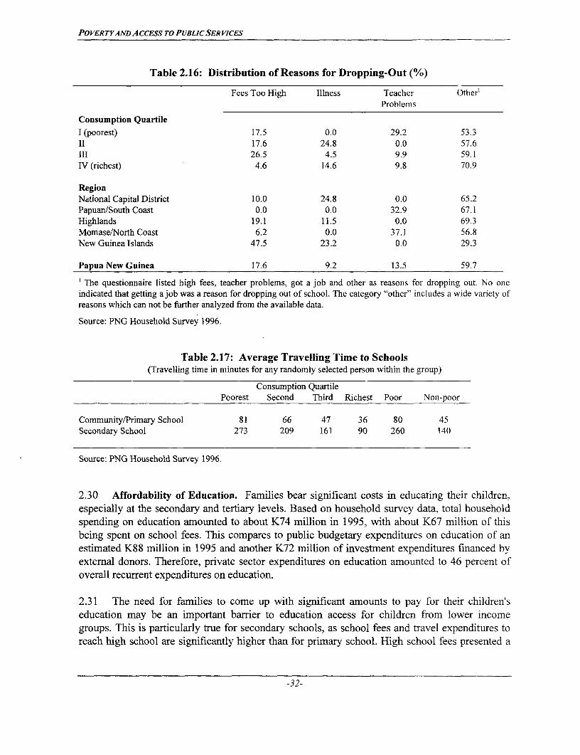
POVERTYANDACCESs TO PUBLICSERviCES
Table 2.16: Distribution of Reasons for Dropping-Out (%)
Fees Too High Illness Teacher Other'
Problems
Consumption Quartile
I (poorest) 17.5 0.0 29.2 53.3
II 17.6 24.8 0.0 57.6
III 26.5 4.5 9.9 59.1
IV (richest) 4.6 14.6 9.8 70.9
Region
National Capital District 10.0 24.8 0.0 65.2
Papuan/South Coast 0.0 0.0 32.9 67.1
Highlands 19.1 11.5 0.0 69.3
Momase/North Coast 6.2 0.0 37.1 56.8
New Guinea Islands 47.5 23.2 0.0 29.3
Papua New Guinea 17.6 9.2 13.5 59.7
' The questionnaire listed high fees, teacher problems, got a job and other as reasons for dropping out. No one
indicated that getting a job was a reason for dropping out of school. The category "other" includes a wide variety of
reasons which can not be firther analyzed from the available data.
Source: PNG Household Survey 1996.
Table 2.17: Average Travelling Time to Schools(Travelling time in minutes for any randomly selected person within the group)
Consumption Quartile
Poorest Second Third Richest Poor Non-poor
Community/Primary School 81 66 47 36 80 45
Secondary School 273 209 161 90 260 140
Source: PNG Household Survey 1996.
2.30 Affordability of Education. Families bear significant costs in educating their children,especially at the secondary and tertiary levels. Based on household survey data, total householdspending on education amounted to about K74 million in 1995, with about K67 million of thisbeing spent on school fees. This compares to public budgetary expenditures on education of anestimated K88 million in 1995 and another K72 million of investment expenditures financed byexternal donors. Therefore, private sector expenditures on education amounted to 46 percent ofoverall recurrent expenditures on education.
2.31 The need for families to come up with significant amounts to pay for their children'seducation may be an important barrier to education access for children from lower incomegroups. This is particularly true for secondary schools, as school fees and travel expenditures toreach high school are significantly higher than for primary school. High school fees presented a
-32-

POVERTY AND A CCESS TO PUBLIC SER VICES
problem among drop-outs for all but the highest quartile and were a particularly important reasonfor dropping out of school in the New Guinea Islands and the Highlands regions. The householdsurvey found that the average outlay on a community school student represents just over 3.5percent of total household non-food expenditure for households in the poorest quartile of thepopulation, while it represents 2 percent of non-food expenditures for households in the richestquartile. For secondary school students, however, the situation is much different: the averageoutlay on a grade 7 or grade 8 student is equivalent to 36 percent of a household's non-foodexpenditure for the poorest quartile of the population, while it amounts to only 6 percent of non-food expenditures for the richest quartile. For grades 9 and 10 the average expenditure perstudent amounts to 42 percent of non-food expenditures of the lowest consumption quartile, butonly 7 percent of non-food expenditures for the richest quartile (Figure 2.4).
Figure 2.4: Affodability of Education(expenditure per student relative to household non-food expenditure)
50%
40% -
30% U Community school20% -Ui t _rC -1 1 Grades 7&8
0 Grade9&10
10%
0%- <
Poorest II Ill Richest
2.32 School fees in PNG vary widely not only across Provinces, but even among childrenattending the same school. One study found that school fees across five villages ranged from K8-K80 per student for grades 1-6 and from K50-K500 for grades 7-8." Such large variations aredue to the fact that schools can set their own fees within parameters provided by each ProvincialGovernment ar,d that fees are in principle expected to be based on a student's ability to pay. Inreality, however, there seem to be substantial inequities in the current fee payment systemwhereby families with similar economic status pay differential amounts. While full uniformity isneither possible nor advisable given the diversity in population, provincial policies and coststructures of education across the country, the Government should undertake to review currentfee payments and policies and develop appropriate guidelines to render the system moreequitable. Special attention should be paid to the treatment of the lowest income groups,particularly in the subsistence sector where availability of cash is often highly restricted.
11 National Research Institute, "Education and the Quality of Life in Papua New Guinea: Five Village Case Studies",Background Paper for Poverty Assessment, Port Moresby, 1996.
-33-
POVERTYAND ACCESS TO PUBLICSER VICES
2.33 Government Education Sector Reform Strategy. To address the key issues whichhave beset PNG's education system, GOPNG has recently launched a major education sectorreform program. The program aims to achieve universal coverage of basic education by 2004, toraise availability of and facilitate access to lower secondary education, and to improve systemefficiency through reduced drop-out rates and improved intra-sectoral resource allocation. Effortsare also under way to increase girls' participation in basic and subsequently secondary education.The program includes a major overhaul of school curricula and a shift to instruction in the locallanguage during the first three years of schooling.
2.34 The program has made a good start, as reflected by rising student enrolment rates in basiceducation, rapid expansion of elementary schools teaching initial grades in local languages andthe growing number of village schools which offer education through grade 8. Continuedsuccessful implementation of the program will be key to improve access to education by the poorand thus help alleviate poverty in PNG. However, these initial successes may be tempered bygrowing capacity constraints at the central and the provincial level. The growth of enrolment hasalso put some strain on the teacher training system and a shortage of elementary school teachersis likely in the years to come. Given the particularly acute shortage of teachers in remote areaswhere achievements of the education system are lowest and poverty concentrations highest,measures are needed to provide teachers with increased incentives to serve in the more remoteand difficult areas.
2.35 Overall budgetary constraints make it unlikely that substantial additional resources willbe available to finance the continued implementation of the education reform program.Therefore, measures which substantially raise the internal efficiency of PNG's education system,such as a reduction in drop-out rates and more efficient deployment of teachers, will be essentialto the continued successful implementation of the program. An intra-sectoral shift in resourceallocation away from higher education towards basic education should accompany efficiencyimprovements.
2.36 The World Bank PNG Education Sector Review estimates that almost one third ofbudgetary expenditures on education currently go to higher education, although higher educationaccounts for only 2 percent of enrolments. This compares to higher education expenditure sharesof 16 percent in Malaysia, Vietnam and Thailand, 19 percent in China and 22 percent in thePhilippines. The highest consumption quartile accounts for 56 percent of higher educationenrolments in PNG, while the lowest quartile accounts for only 9 percent of enrolments. Thisthus means that the high share of public monies going to higher education primarily benefits theupper income groups. Given sectoral resource constraints and the need to substantially raiseenrolments in basic education, particularly among the lower income groups, a more efficient andequitable allocation of sectoral resources is essential. To help guide the reallocation of intra-sectoral resources, a detailed review of public expenditures in the education sector should becarried out. Such a review should include an analysis of the distributional impact of public
-34-
POVERTYAND ACCESS TO PUBLICSERVICES
education sector expenditures on various income groups.2 While fees payments will have toremain an important part of school financing in the foreseeable future, the fees payment systemneeds to be overhauled to introduce better consistency and equity and to improve access of thepoor to basic education.
D. RURAL INFRASTRUCTURE
2.37 Access to transport infrastructure is an important determinant of economic welfare inPNG. The proximity of all-weather roads or shipping facilities is associated with the existence ofpermanent markets, enterprises, labor mobility, diversification and overall higher livingstandards. Access to transport infrastructure makes it easier to gain access to markets for finalgoods and services, to sources of productive inputs, to social services and to alternativeemployment.
2.38 Although PNG compares relatively favorably with other developing countries in termsof meters of road per person and per square kilometer, a vast majority of roads are poorlymaintained and inaccessible during and after rains13 . Together with the poor integration amongdifferent modes of transportation (road, water, air), this results in a highly fragmented andunreliable transportation system and high transportation costs. There is a marked difference inaccess to transportation infrastructure between income groups (Table 2.18). The lowestconsumption quartile must travel over twice as long to gain access to the closest mode oftransport than the richest quartile. The poor travel 75 percent longer than the non-poor to theclosest mode of transportation and over three times longer to reach the closest road. A simpleregression of per capita consumption against travelling time to the nearest transport facilityshows that consumption is highly correlated with access to transportation. A one hour increase intravelling time to the nearest transport facility reduces real consumption by 10 percent (Figure2.5). This suggests that measures which improve rural communities' access to transportinfrastructure will be an important aspect of poverty alleviation in PNG.
2.39 Data from the household survey confirm that PNG's population, particularly the lowerincome groups, rank investments in rural infrastructure as the highest priority for externalinterventions. Maintenance of existing roads, construction of new roads and provision ofimproved water supply were the three highest priorities for external investments mentioned bythe vast majority of the population, including the poor.
12 The lack of detailed education sector expenditure information prevented such an analysis in the context of thisreport.
13 According to the Road Inventory and Road Maintenance study, only 46 percent of national paved roads and 37percent of national unpaved roads were in satisfactory condition. Country-wide only 27 percent of the existingroad network were deemed to be in good condition in 1995 and the situation is likely to have deteriorated sincethen..
-35-
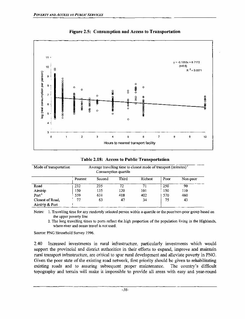
POVERTYAND ACCESS TO PUBLICSERViCES
Figure 2.5: Consumption and Access to Transportation
1t1l
y -0.1053x + 6-7172
10 (t=6.6)1 8 R 2 = 0.0371
0
0 0
C 0 ~000L 0
a 0~~~02 00
0~~~~~~~~ C' 7 oE7 8 § l-
.2 0~~ 0
4-
3-
0 1 2 3 4 5 6 7 8 9 10
Hours to nearest transport facility
Table 2.18: Access to Public Transportation
Mode of transportation Average travelling time to closest mode of transport (minutes)'Consumption quartile
Poorest Second Third Richest Poor Non-poor
Road 232 235 72 71 250 90Airstrip 150 135 120 101 150 110Port2 559 631 418 402 570 460Closest of Road, 77 63 47 34 75 43Airstrip & Port
Notes: 1. Travelling time for any randomly selected person within a quartile or the poor/non-poor group based onthe upper poverty line
2. The long travelling times to ports reflect the.high proportion of the population living in the Highlands,where river and ocean travel is not used.
Source: PNG Household Survey 1996.
2.40 Increased investments in rural infrastructure, particularly investments which wouldsupport the provincial and district authorities in their efforts to expand, improve and maintainrural transport infrastructure, are critical to spur rural development and alleviate poverty in PNG.Given the poor state of the existing road network, first priority should be given to rehabilitatingexisting roads and to assuring subsequent proper maintenance. The country's difficulttopography and terrain will make it impossible to provide all areas with easy and year-round
-36-

POVERTYANDACCESS TO PuBLiCSERViCES
access to transportation. Apart from modest investments in rural tracks, investments in newtransportation facilities should be carefully considered for their economic viability. Substantialinvestments in isolated areas with very low population densities may well not turn out to beviable and a policy which over time encourages out-migration from such areas may be a moreeffective means to alleviate poverty. In the short run, alternative interventions aimed atalleviating poverty are needed in such areas. Improved access to basic education can help peoplein such communities build up their human capital in view of eventual out-migration. Othermeasures include small-scale infrastructure investments which can facilitate living conditions inisolated communities, particularly in the areas of rural water supply, basic health services andrural tracks.
2.41 To properly target small-scale infrastructure investments and assure effectiveparticipation by the local communities (which is a precondition for sustainability of suchinvestments), specific projects should be identified and implermented with the participation ofbeneficiary communities. This requires that local governments be strengthened in their capacityto identify, design and implement such projects and be provided necessary additional fundingfrom the central government budget. It also requires that the capacity of local governments todirectly work with beneficiary communities be strengthened and/or that these governments enterinto a partnership with NGOs that are experienced in effectively working with localcommunities.
2.42 To assure effective local participation and sustainability of small-scale rural infrastructureinvestments, the establishment of local investment fund arrangements should be considered.Such funds could provide financing for small scale investments for communities willing toparticipate and contribute to a particular project of importance to them. Operation of such fundscould conceivably be modeled on the functioning of Social Investment Funds which havesuccessfully helped alleviate poverty and mobilize local communities in many parts of theworld"4. Under such an arrangement the National Government (or an independent nationalagency) would provide assistance with project design and strict guidelines for eligibility.Eligibility might be limited to the poorest provinces with a good track record of implementingsocial services and collaborating with local communities. Beneficiary communities would beclosely involved in all phases of project planning and implementation and be required to make acontribution to the investment. Public agencies in charge of such funds should avail themselvesof the help or delegate actual implementation of such initiatives to NGOs and other private sectoragencies (including church services) which have a proven track record of successfully assistingcommunities with the implementation of such projects.
4 Examples of schemes which have successfully supported local development initiatives while strengthening localcommunities' ability to take charge include Social Investment Funds in Latin America, the FSU and morerecently also a number of Asian countries, as well as rural development projects which provide block grants tocommunities for small scale infrastructure and other initiatives in Indonesia and the Philippines.
-37-
POVERTYANDACCESS TO PUBLICSER VICES
E. LIVING STANDARDS AND ACCESS TO PUBLIC SERVICES
2.43 Proper access to basic public services can influence a person's welfare on at least twoaccounts: first, the use of such services can improve the person's overall and physical well-beingand second, the availability of such services can substantially increase a person's ability to earnhigher incomes. Standard regression analysis was used to measure the extent to which ahousehold's economic welfare is influenced by access to basic public services, controlling forother variables, such as household size, income souirce, fixed regional effects and age of thehousehold head (see Annex VI for details).
2.44 The analysis confirmed that years of schooling, literacy, access to transportation, marketsand health services are all important predictors of houisehold consumption, even when householdsize, age of the household head, income source, household agricultural assets, geo-climatic andregional effects were controlled for (see Annex VI).
2.45 The results of the regression analysis were then used to simulate the impact of changes inkey variables on the headcount index of poverty in P`G. These simulations should not be usedfor detailed policy prescriptions.'5 Nonetheless, the simulations do suggest that poverty in PNGcould be reduced in both urban and rural areas if access to schooling, health services, marketsand roads were improved.
F. DECENTRALIZATION AND PROV[SION OF BASIC SERVICES
2.46 The provincial reforms which PNG launched in 1995 have so far failed to improveservice delivery at the local level and it is widely believed that they have had a disruptive effect.The decentralization efforts have resulted in a situation where central agencies are no longer in aposition to deliver services and their management capacity has broken down, while local levelagencies often lack the human and financial resources to properly carry out their tasks. Theprovincial reforms have been afflicted by a number oi factors, including insufficient leadershipand monitoring by central government agencies, finaacial problems, inadequate personnel andinfrastructure at local level, and lack of community involvement.
2.47 Provincial reforms were rushed and inadequately prepared. Provincial and localgovernments have largely been left on their own to figure out how service delivery should beorganized and carried out at the local level. Furthermore, provincial and local governments have
5 Two potential caveats should be mentioned: the possibility of endogenous program placement, and the fact thatthere may be aggregation problems. If health posts or schools are placed in areas in which there is greaterdemand for health or education, the estimates from these simulations may be biased up; conversely, if they aretargeted towards poorer areas, and if poverty is not fully captured by other controls in the regression, theestimates from these simulations may be biased down. Second, the simulations are based on partialequilibrium models, and therefore take into account only airst-order changes. For example, the aggregateeffect of a large change in literacy may be different from that predicted in the simulations as the economyadjusts to an influx of more skilled labor.
-38-

POVERTYAND ACCESS TO PUBLICSER VICES
Table 2.19: Simulated Effect of Certain Changes on Incidence of Poverty
Headcount index(Percent change from base)
Rural Urban PNGBaseline: Actual values 33.51 11.41 30.17
Baseline: Predicted values 32.76 9.83 29.30
Increase household average school years per 31.55 7.83 27.97adult by one year (-3.69) (-20.35) (-4.54)
Increase literacy rate of household heads to 27.28 9.22 24.55100 percent (-16.72) (-6.14) (-16.19)
Decrease number of unemployed adults so at 32.31 9.39 28.85least 50 percent of adults per household earn (-1.38) (-4.41) (-1.53)cash
Increase number of pigs owned per 31.82 10.14 28.54household by one (-2.89) (3.23) (-2.58)
Increase index of market development by 32.34 n.a. 28.9410 percent (-1.29) (-1.22)
Decrease travelling time to nearest road by 31.85 n.a. 28.5250 percent (-2.78) (-2.64)
Decrease travelling time to road to 3 hours 31.44 n.a. 28.17for communities where currently > 3 hours (-4.05) (-3.84)
Decrease travelling time to road to 2 hours 31.34 n.a. 28.09for communities where currently > 2 hours (-4.35) (4.13)
Decrease combined travelling time to 3 key 31.61 3.49 27.36social services by 50 percenta (-3.51) (-66.51) (-6.60)
Decrease combined travelling time to 3 key 31.32 n.a. 28.07services to 6 hours if currently > 6 hours (-4.40) (-4.18)
Note: Headcount index calculated as the weighted average of the predicted probability that each household ispoor, following a simulated change, where the weights are the household sampling weights multiplied bythe number of persons in the household. Model used to predict poverty of rural households reported inTable 3 of Annex 5 and model for urban households reported in Table 6 of Annex 5. The percent changefrom base is calculated from the predicted baseline values.
aHealth center, high school and government station.
Source: Annex VI.
-39-
POVERTYAND ACCESS TO PUBLICSERVICES
in many cases been given additional responsibilities, without being provided with the necessaryfinancial resources to carry them out. As a result, many important programs, particularly in thesocial sectors and in the area of infrastructure development and maintenance have remainedunderfunded. This has led to a marked reduction of service delivery, particularly in poorer areas.Many district and local governments have not been able to recruit and retain adequately trainedstaff to assume the increased responsibilities which have been placed on them as a result ofdecentralization. A centrally determined and unified salary scale for public servants has made itvirtually impossible for local agencies in remote areas to attract well qualified staff, because thescale does not allow for any premium payments in difficult service areas. As a result, manyremote areas have remained without the necessary staff to provide them with basic health andeducation services.
2.48 Decentralization can improve the provision of basic services to the population if it isproperly planned, implemented and funded. The central government must assume a leadershiprole in this effort. Decentralization should not be launched until detailed implementationguidelines have been prepared for local governments and the central government is ready toprovide adequate guidance throughout implementation. It is also the central government'sresponsibility to see to it that decentralization does not result in a situation where serviceprovision in poorer regions lags substantially behind that in wealthier areas because poorerregions lack the funding to provide basic social services. To improve basic service delivery inPNG, the achievements of and problems afflicting decentralization need to be carefully reviewedso that corrective measures can be taken. Box 5 outlines key aspects which need to be consideredwhen the provision of social services is decentralized.
-40-
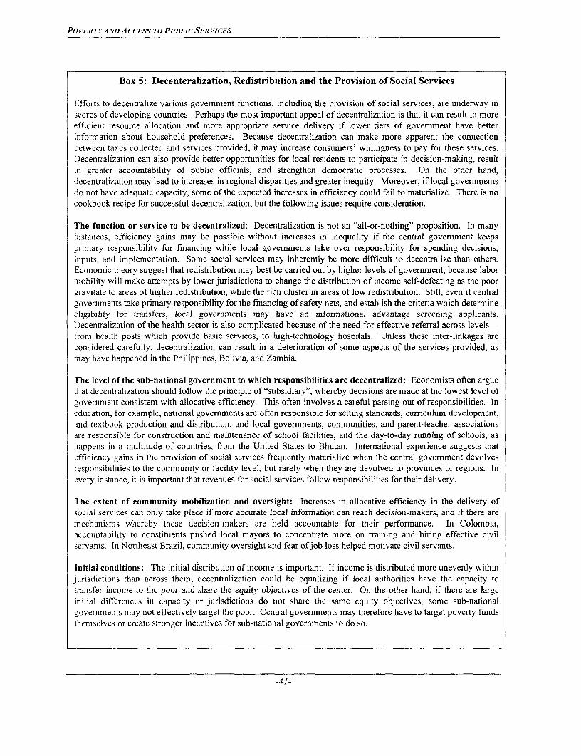
PO VERTY AND ACCESS TO PUBLIC SERVICES
Box 5: Decenteralization, Redistribution and the Provision of Social Services
Efforts to decentralize various government functions, including the provision of social services, are underway inscores of developing countries. Perhaps the most important appeal of decentralization is that it can result in moreefficient resource allocation and more appropriate service delivery if lower tiers of government have betterinformation about household preferences. Because decentralization can make more apparent the connectionbetween taxes collected and services provided, it may increase consumers' willingness to pay for these services.Decentralization can also provide better opportunities for local residents to participate in decision-making, resultin greater accountability of public officials, and strengthen democratic processes. On the other hand,decentralization may lead to increases in regional disparities and greater inequity. Moreover, if local governmentsdo not have adequate capacity, some of the expected increases in efficiency could fail to materialize. There is nocookbook recipe for successful decentralization, but the following issues require consideration.
The function or service to be decentralized: Decentralization is not an "all-or-nothing" proposition. In manyinstances, efficiency gains may be possible without increases in inequality if the central government keepsprimary responsibility for financing while local governments take over responsibility for spending decisions,inputs, and implementation. Some social services may inherently be more difficult to decentralize than others.Economic theory suggest that redistribution may best be carried out by higher levels of government, because labormobility will make attempts by lower jurisdictions to change the distribution of income self-defeating as the poorgravitate to areas of higher redistribution, while the rich cluster in areas of low redistribution. Still, even if centralgovernments take primary responsibility for the financing of safety nets, and establish the criteria which determineeligibility for transfers, local governments may have an informational advantage screening applicants.Decentralization of the health sector is also complicated because of the need for effective referral across levels-from health posts which provide basic services, to high-technology hospitals. Unless these inter-linkages areconsidered carefully, decentralization can result in a deterioration of some aspects of the services provided, asmay have happened in the Philippines, Bolivia, and Zambia.
The level of the sub-national government to which responsibilities are decentralized: Economists often arguethat decentralization should follow the principle of "subsidiary", whereby decisions are made at the lowest level ofgovernment consistent with allocative efficiency. This often involves a careful parsing out of responsibilities. Ineducation, for example, national governments are often responsible for setting standards, curriculum development,and textbook production and distribution; and local governments, communities, and parent-teacher associationsare responsible for construction and maintenance of school facilities, and the day-to-day running of schools, ashappens in a multitude of countries, from the United States to Bhutan. International experience suggests thatefficiency gains in the provision of social services frequently materialize when the central government devolvesresponsibilities to the community or facility level, but rarely when they are devolved to provinces or regions. Inevery instance, it is important that revenues for social services follow responsibilities for their delivery.
The extent of community mobilization and oversight: Increases in allocative efficiency in the delivery ofsocial services can only take place if more accurate local information can reach decision-makers, and if there aremechanisms whereby these decision-makers are held accountable for their performance. In Colombia,accountability to constituents pushed local mayors to concentrate more on training and hiring effective civilservants. In Northeast Brazil, community oversight and fear of job loss helped motivate civil servants.
Initial conditions: The initial distribution of income is important. If income is distributed more unevenly withinjurisdictions than across them, decentralization could be equalizing if local authorities have the capacity totransfer income to the poor and share the equity objectives of the center. On the other hand, if there are largeinitial differences in capacity or jurisdictions do not share the same equity objectives, some sub-nationalgovernments may not effectively target the poor. Central governments may therefore have to target poverty fundsthemselves or create stronger incentives for sub-national governments to do so.
-41-

POVERTYAND ACCESS TO PUBLIC SERVICES
3. SOCIAL SAFETY NETS
A. INTRODUCTION
3.1 The basic elements of an effective poverty alleviation strategy are economic growth andinvestments in human capital. However, regardless of how well such strategies succeed, therewill always be some who will not be able to fully participate. First, it may take too long forsome, particularly those in very remote areas, to fully participate and certain groups like the oldor disabled may never be able to do so. Second, even among those who will benefit from thesepolicies, there will be some who remain acutely vulnerable to adverse events, such as temporaryunemployment, natural calamities or death. In many countries, including PNG, there are informalcommunity or family based arrangements which help those in need cope. However, there arelimits to what such informal arrangements can do to protect the most needy. In particular, copingarrangements which work well in normal times, may fail to provide the necessary relief duringshock situations. The effectiveness of community-based insurance depends strongly on the extentto which local incomes are affected simultaneously. Unanticipated shock resulting from naturaldisasters, deterioration of terms of trade or famine can leave entire communities unable to copeon their own.
3.2 There is therefore a role for Government to assist vulnerable households and communitiesin the face of shock and to ensure minimal levels of provision to those who are unable to benefitfrom generalized poverty alleviation policies. The latter group is generally best protected throughsome form of income transfer scheme, while those in need in the face of shock are best aidedthrough some sort of insurance scheme. Successful Government policies in both areas will needto assess what informal arrangements exist and how effective they are. They will then attempt tostrengthen or supplement such informal arrangements rather than displace them.
B. INFORMAL SOCIAL SAFETY NETS
3.3 The most widespread informal social safety net in PNG is the wantok system"6. Thissystem allows for income transfers and other support from members of a particular wantok toneedy members of the same wantok. In rural areas wantok systems are generally based onkinship. In urban areas they often have a broader base which may include kinship, place oforigin, ethnicity, language, place of residence or merely friendship. Wantoks which span acrossurban and rural areas are generally also based on kinship.
3.4 The household survey has found that inter-household income transfers remain a veryimportant means of assisting households. Over 90 percent of households received transfers andover 90 percent of households made transfers. Income transfers (both on the receiving and thegiving side) were important across all income groups and in all geographic regions. Although theshare of households making transfers declined somewhat as consumption decreased, over 80
16 Wantok is Pidgin English for "one talk", i.e. a group of people speaking the same language.
-42-
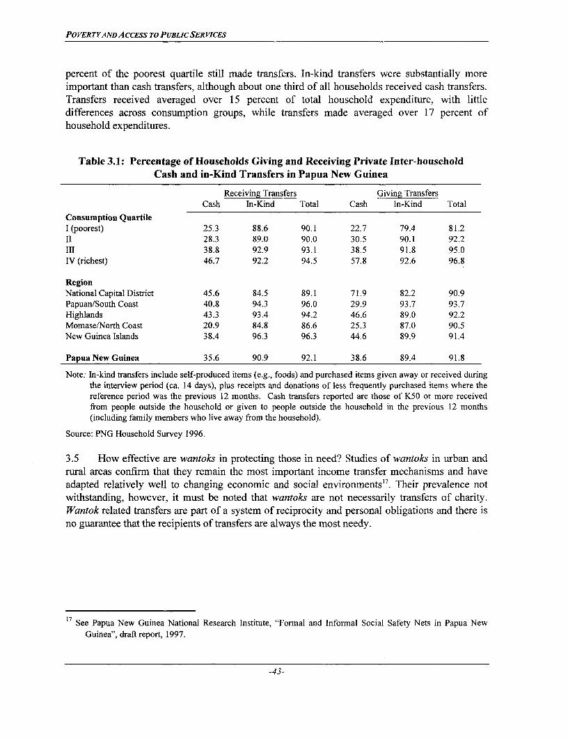
POVERTYAND ACCESS TO PUBLIC SERVICES
percent of the poorest quartile still made transfers. In-kind transfers were substantially moreimportant than cash transfers, although about one third of all households received cash transfers.Transfers received averaged over 15 percent of total household expenditure, with littledifferences across consumption groups, while transfers made averaged over 17 percent ofhousehold expenditures.
Table 3.1: Percentage of Households Giving and Receiving Private Inter-householdCash and in-Kind Transfers in Papua New Guinea
Receiving Transfers Giving Transfers
Cash In-Kind Total Cash In-Kind Total
Consumption Quartile
I (poorest) 25.3 88.6 90.1 22.7 79.4 81.2
II 28.3 89.0 90.0 30.5 90.1 92.2
III 38.8 92.9 93.1 38.5 91.8 95.0
IV (richest) 46.7 92.2 94.5 57.8 92.6 96.8
Region
National Capital District 45.6 84.5 89.1 71.9 82.2 90.9
Papuan/South Coast 40.8 94.3 96.0 29.9 93.7 93.7
Highlands 43.3 93.4 94.2 46.6 89.0 92.2
Momase/North Coast 20.9 84.8 86.6 25.3 87.0 90.5
New Guinea Islands 38.4 96.3 96.3 44.6 89.9 91.4
Papua New Guinea 35.6 90.9 92.1 38.6 89.4 91.8
Note: In-kind transfers include self-produced items (e.g., foods) and purchased items given away or received during
the interview period (ca. 14 days), plus receipts and donations of less frequently purchased items where the
reference period was the previous 12 months. Cash transfers reported are those of K50 or more received
from people outside the household or given to people outside the household in the previous 12 months
(including family members who live away from the household).
Source: PNG Household Survey 1996.
3.5 How effective are wantoks in protecting those in need? Studies of wantoks in urban andrural areas confirm that they remain the most important income transfer mechanisms and haveadapted relatively well to changing economic and social environments"7 . Their prevalence notwithstanding, however, it must be noted that wantoks are not necessarily transfers of charity.Wantok related transfers are part of a system of reciprocity and personal obligations and there isno guarantee that the recipients of transfers are always the most needy.
17 See Papua New Guinea National Research Institute, "Formal and Informal Social Safety Nets in Papua New
Guinea", draft report, 1997.
-43-

POVERTY AND ACCESS TO PUBLIC SERviCES
Table 3.2: Average Value of Private Inter-household Cash and in-Kind Transfers as aPercentage of Total Household Expenditure in Papua New Guinea
Transfers Received Transfers GivenCash In-Kind Total Cash In-Kind Total
Consumption QuartileI (poorest) 2.4 12.8 15.2 3.4 13.9 17.4II 3.1 12.3 15.3 3.7 12.7 16.4III 2.5 13.2 15.8 3.1 17.5 20.5IV (richest) 2.8 12.6 15.4 3.3 15.0 18.4
RegionNational Capital District 2.0 7.7 9.6 3.8 6.9 10.7Papuan/South Coast 2.3 11.8 14.1 1.5 20.0 21.5Highlands 3.3 14.4 17.6 5.0 16.1 21.1Momase/North Coast 2.2 10.8 13.0 1.7 11.2 12.9New Guinea Islands 3.0 15.7 18.7 4.4 10.9 15.4
Papua New Guinea 2.7 12.7 15.4 3.4 14.1 17.5
Notes: See Table 3.1 for details on how the data were collected. It appears that respondents either forget sometransfers received or put a higher value on the transfers they make compared with the transfers they receivebecause the reported value of transfers given exceeds the reported value of transfers received.
Source: PNG Household Survey, 1996.
3.6 Statistical analysis of the pattern of transfer receipts in the household survey datasuggests that informal transfers in the rural sector of PNG leave the distribution of incomeunchanged - in other words, they are not directed mainly from rich households to poorerhouseholds (see Annex VII for details). This is also apparent in the aggregate data (which isdominated by the rural sector) in Table 3.2 which shows that transfer receipts have an almostconstant ratio to household expenditures across consumption quartiles. In contrast, transferreceipts in the urban sector do indicate some aversion to inequality on the part of donors, so thedistribution of income in the urban sector is made more equal by the wantok system.
3.7 In both the urban and rural sectors, transfer receipts are higher for female-headedhouseholds and this may explain why the household survey found that female-headed householdswere no poorer than other households. In the rural sector, transfer receipts are also higher (andtransfer outlays lower) for households where a baby was born in the past year and for householdswhere the head has no sources of cash income. However, these patterns were not apparent in theurban sector. Somewhat surprisingly, transfer receipts do not seem to be higher for olderhouseholds or in the case of illness (see Annex VII for details). One factor which might helpexplain why transfer receipts for older households or households afflicted by illness are nothigher is that transfer receipts recorded by the household survey were limited to transfers in cashand in kind. However, particularly in rural settings, transfers of labor, childcare and garden worksharing are very common and are likely to particularly benefit the elderly and the sick. Whilesuch transfers would not have been recorded by the household survey, they are an important partof the informal social safetynet.
-44-

POVERTYANDACCESS TO PUBLIC SER VICES
3.8 Thus, the overall pattern of these results suggests that income transfers made under thewantok system may respond to particular shocks and types of disadvantage in the rural sector,whilst not having any overall effect on the distribution of income. In the urban sector, thesetransfers are targeted towards the poor, but they don't appear to increase with the age of thehousehold head or in the case of illness. The elderly and the sick may, however, well benefitfrom other transfers, particularly transfers of labor.
3.9 Another geographically more limited analysis of wantoks in an urban setting showed thatvoluntary transfers of cash made on a regular basis were targeted towards the poor and thathouseholds received more transfers if they suffered from a sudden misfortune in the form of lostincome. The study also confirmed that wantoks and thus voluntary inter-household transfersremain important for households who have access to formal credit and insurance facilities".
3.10 There is considerable debate about whether the wantok system operates as an effectivesafety net and redistributive force in urban squatter settlements. Observers of these squatter areasnote that the population may have lost all ties to their place of origin and may have no wantoksliving close by who can help them in times of need. But proposals to supplement the informalsafety net with formal interventions remain controversial because of concern about the incentivescreated for the formation of new squatter areas. A detailed statistical analysis of urban householdsurvey data from the 1980s suggests that households in urban squatter areas are more likely toparticipate in the giving or receiving of private inter-household transfers than are other urbanhouseholds. Multivariate modelling of the pattern of transfer receipts across householdssuggested that transfers in urban squatter settlements were not quite as well targeted towards thepoor as they were in the non-settlement urban areas but they still acted to reduce inequality.Moreover, there was no difference between squatter and non-squatter areas in the net flow ofprivate transfers towards households headed by the elderly or those in ill-health orunemployment. Households in squatter areas also appeared more willing than non-settlementhouseholds to raise their outlays on transfers to wantoks as their own incomes rose.'9 Thus, theoverall picture from this statistical analysis is not one of the wantok system being less effectivein urban squatter areas than it is in other urban areas.
3.11 The importance of wantoks not withstanding, there are limits to what these systems canachieve. In communities which are characterized by very high poverty rates, the possibilities forinter-household transfers remain limited by low household incomes. In times of shock,particularly those brought about by natural disasters, community support arrangements often fail,unless the community includes a substantial number of wantok members outside the affected area(such as urban dwellers). There is thus a need to supplement these informal safety netarrangements with limited formal interventions.
18 See Gibson, J. G. Boe-Gibson and F. Scrimgeour, (1998), "Are Voluntary Transfers and Effective Safety Net inUrban Papua New Guinea?", Mimeo.
19 Gibson, J, (1999 d), "Are There Holes in the Safety Net? Private Transfers in Squatter Settlements and OtherUrban Areas of Papua New Guinea", Mimeo.
-45-
POVERTYAND ACCESS TO PUBLIC SER VICES
3.12 What is the most effective way to supplement informal safety nets? An analysis of socialsafety net arrangements in PNG carried out by the National Research Institute, identified threetypes of measures could that effectively complement and support PNG's informal social safetynet structures.20 The three interventions identified by this study include: (i) targeted incometransfers in the form of free or substantially subsidized health and education services to thosewho are most at risk and disadvantaged (single parents, families with many children,unemployed); (ii) improved provision of government and NGO funded emergency and reliefservices, which would assure that relief efforts in response to natural disasters effectively reachthose in need, and (iii) investments in basic social services and rural infrastructure to spur overalleconomic growth and improve welfare, particularly in areas with substantial poverty. This in turnwould provide existing wantoks with increased means to assist those in need. Finally, the studyunderlined that no attempts should be made to directly strengthen wantok systems per se, as suchinterventions might result in their disintegration. Rather, conditions should be established forwantoks to effectively operate in an overall improved economic environment.
C. FORMAL SOCIAL SAFETY NETS
3.13 PNG has several formal safety net arrangements which operate with varyingeffectiveness. Among them are: (i) wage-linked social security/insurance schemes; (ii) pricesupport schemes; (iii) social development schemes; and (iv) emergency relief actions.
3.14 The wage-linked social security schemes include the National Provident Fund, thePublic Officers Superannuation Fund and the Defense Force Retiree Benefit Fund. Theseschemes provide an effective safety net for wage earners and their families in the formal and thepublic sector. They provide unemployment, old age, disabled and survivor benefits to theirparticipants. While effective safety net mechanisms, these funds are limited to formal and publicsector wage earners, mainly in urban areas, and do thus not benefit the vast majority of thosewho either are poor or are at risk of being poor.
3.15 Furthermore, all three funds have experienced a significant deterioration in their financialperformance and coverage over the past few years. These difficulties are due to a number offactors, including the lack of prudential supervision and regulation, poor investments,Government use of pension funds for capital investments of questionable quality, politicalinterference as reflected by the frequent replacement and appointment of board members andmanaging directors for political reasons rather than for their qualifications and expertise, andlarge Government arrears to the fund for public sector employees. The future effectiveness ofthese funds as safety net mechanisms for those employed by the formal sector thus requires aseries of reforms. Among them are the urgent need to establish a body to regulate and supervise
20 See Papua New Guinea National Research Institute, "Formal and Informal Social Safety Nets in Papua NewGuinea", draft report, 1997.
-46-
POVERTYAND ACCESS To PUBLIC SER VICES
these funds, the adoption of superannuation legislation, measures to improve governance andincrease accountability and revoking the power of the Government to issue investment guidelinesto these funds.21
3.16 Price Support Schemes. PNG has had a long history of price stabilization and/or pricesupport schemes for its major export crops, coffee, copra, cocoa and palm oil. The idea behindthese schemes was that they would help protect producers of these crops from fluctuations inworld market prices and thus smooth their income. The schemes were to pay growers a bonusduring times of low world market prices. This bounty was to be financed through levies collectedduring times of high commodity prices. Through the end of the 1980s these schemes wereessentially self-financing. However, with the collapse of world market commodity prices in thelate 1980s, the stabilization funds became essentially insolvent and were replaced withGovernment-assisted export price support programs. These Government financed schemes wereextremely costly and ill targeted. The average annual expenditures during the first half of the1990s amounted to over two thirds of the Department of Agriculture and Livestock's overallbudget in support of agricultural development.22 The fiscal burden of maintaining these schemesproved to be unsustainable. Furthermore, while these schemes did help smooth income of someexport crop producers, the bulk of the benefits accrued to owners of large estates rather thansmall holders. Overall, agricultural price support schemes were not an effective means to helpprevent poverty. As the household survey shows, poverty remains widespread among small scaletree crop producers. Given resource constraints, the funds allocated to such schemes would beused more effectively to help spur agricultural and rural development through investments inrural infrastructure and basic social and agricultural support services.
3.17 Social Development Schemes: The most prominent scheme is the Rural ActionProgram, also referred to as Electoral Development Fund. The scheme started in the late 1970s asthe Village Development Fund and was meant to provide grant and loan based assistance tovillagers with viable project proposals and willing to make a 30 percent contribution of theirown. The scheme, however, soon got transferred into a fund for Parliamentarians who distributedresources to their electorate at will. More recently the fund has been put under the administrationof the District Planning Committee, of which the local member of Parliament is the chairman.The fund has no obligations to regularly report on its use of funds. Some allocations have beenmade to those in need in the form of income subsidies, assistance with education or medicalexpenses and assistance to disaster-stricken families. Other uses include contributions tocommunity development projects. Overall, however, this fund is hardly an effective social safetynet mechanism. There are no clear criteria to define target beneficiaries nor are there clear rulesabout how to obtain these funds and what they can finance. To become an effective povertyalleviation mechanism, this fund should either be transferred into a true social assistance scheme
21 For further details, see World Bank, (1999b), Papua New Guinea: Country Economic Memorandum, draft, June,
1999.
22 See, World Bank, (1997), Papua New Guinea: Accelerating Agricultural Growth - An Action Plan, WashingtonDC.
-47-

POVERTYAND ACCESS TO PUBLICSERVICES
which is administered based on well defined, transparent rules and criteria or it should be turnedinto a local development or public employment schemes fund (see para. 3.20).
3.18 Disaster Relief Mechanisms. Both Government and NGOs have mechanisms to providerelief to communities struck by natural disaster. The Government's program is carried out by theNational Disaster and Emergency Service, while that of the NGOs is carried out by a number ofNGOs, including the Red Cross, Salvation Army and St. John Ambulance. While these serviceshave certainly provided much-needed relief to many communities and families touched bynatural calamities, their operations overall often suffer from limited technical know-how, lack ofwell developed emergency relief operational plans and underfunding.
3.19 PNG has a wide-spread informal social safety net which covers a vast majority of thepopulation. Although transfers under this system to not appear to improve rural incomedistribution, they do seem to provide protection against certain types of shock. In urban areasthey also appear to be targeted towards the poor. Low income levels, particularly in the moreisolated communities, and unforeseeable events, however, put limits on how much the informalsafety net can protect those in need. There is thus a need for the Government to supplement theinformal safety net with well-targeted interventions. In particular, the possibility of providingpoor families with many children with assistance to meet basic education and health expendituresshould be considered. However, effective targeting, particularly when only certain groups (asopposed to entire regions) are selected, involves significant administrative efforts and costs, andthe best way of selecting beneficiaries for such benefits in PNG needs to be evaluated carefully.It is highly unlikely that formal means tests could effectively be employed for this purpose inPNG. Therefore, alternative means, such as household characteristics will have to be employed.The data from the household survey have shown that the level of schooling of the householdhead and the main income source of the household may be possible selection indicators fortargeting of such benefits.
3.20 An alternative way to provide those in need with support would be through self-targetedwork-fare schemes. Such programs would provide unskilled low-wage work on demand at awage rate low enough to guarantee that only those in real need are willing to participate. Thelabor would be used to build and maintain high priority community infrastructure in poor areas.Communities in designated target areas would be given the opportunity to propose small-scaleinfrastructure works for funding under the program. If a proposed project met a set of basicselection criteria, the work-fare program would pay for labor and in poorer areas possibly somematerial costs of executing the scheme. Participation would be open to all who are willing towork for the wage paid by the program. Participation would need to be limited to a maximumnumber of days per worker, so as to assure that the available financial resources are sufficient toprovide work to all those who are willing to work under the scheme at the prevailing low wagerate. If properly designed and funded, work-fare schemes are an effective safety net mechanismto help alleviate chronic and transient poverty (e.g. poverty resulting from natural disaster,economic shocks etc).
3.21 Assistance for disaster-struck areas will remain critical in PNG. The agencies to providesuch assistance would benefit from support to strengthen their technical and planning capacities.
-48-

POVERTYAND ACCESS TO PUBLIC SER VICES
Schemes such as agricultural price supports or the Rural Action Program are not effectivepoverty alleviation mechanisms, nor good safety nets. These are costly operations which are notwell targeted and should thus be replaced by more appropriate mechanisms either in support ofoverall rural development or to provide well targeted social assistance benefits. The wage-linkedsocial insurance schemes, although only benefiting a small part of the population, are animportant safety net mechanism and will grow in importance as the country develops further anda larger share of the labor force will enter the formal labor market as wage earners. However,their future effectiveness will largely depend on the Government's ability to implement a seriesof measures to strengthen the financial performance of these funds.
-49-

POVERTYAND ACCESS TO PUBLICSER VICES
4. INFORMATION GAPS AND FURTHER ANALYSIS TOGUIDE POVERTY ALLEVIATION POLICIES
A. INFORMATION GAPS AND ADDITIONAL ANALYSIS
4.1 The data collected during the first nationally representative household survey hasallowed to produce a poverty profile for PNG and to see to what extent the lower incomegroups have access to basic social services. The data has shown that about 37 percent ofPNG's population are poor if an average national poverty line of 461 kina per adultequivalent per year (1996 prices) is used. Compared to countries with similar incomelevels, poverty in PNG is high. Poverty alleviation thus remains an importantdevelopment challenge in PNG. Broad based economic growth2 3 and improved provisionof public services, including rural infrastructure, will be key ingredients of a povertyalleviation strategy in PNG. To further guide Government interventions in favour ofpoverty alleviation, additional analysis will be required on several fronts.
4.2 Agricultural production: The vast majority of PNG's poor are either subsistenceor small- scale tree crop producers. Therefore, a successful anti-poverty strategy willneed to help these producers increase their productivity, integrate into the marketeconomy and diversify income sources. To formulate proper interventions which canfacilitate this process, an analysis of access to and use of land, rural credit and productionissues faced by small scale producers in various agro-ecological zones is necessary. Thiswill require that future household surveys include data on land holdings and utilization,agricultural production, access to agricultural support services and markets. In addition,more needs to be understood about the technology base and options for long termproductivity increases for many of the crops produced by PNG's small-scale farmers.This in turn requires a detailed analysis of the production systems in various agro-ecological zones of PNG, particularly the Highlands and Momase/North Coast whichaccount for over 75 percent of poverty in PNG. Such analysis will need to be paralleledwith proper agricultural research to build up the technology base for productivityincreases.
4.3 Effectiveness of Public Spending on Health and Education. The household surveyhas clearly shown that the lower income groups do not have proper access to basiceducation and health services and that PNG's population is dissatisfied with its access topublic services. There is significant inter-regional variation in the performance of thehealth and education systems. The poor performance of the health and education systemsare at least partly due to inadequate levels and erratic flows of public funding. It is likelythat the regional variation in performance is also influenced by differences in fundinglevels and in the effectiveness of sectoral resource allocation between provinces. Manycountries with poor or falling health performance indicators have found that areallocation of public expenditures in line with the population's health needs couldsubstantially help increase the sector's performance and improve the lower income
23 As the past has shown, economic growth will only markedly benefit the lower income groups if it is notaccompanied by a worsening in the income distribution.
-50-

POVERTYAND ACCESS TO PUBLIC SERVICES
access to health care. The same applies to education. It is therefore of great importance that theuse of public expenditures for health and education in PNG be closely monitored.
4.4 Public expenditures for the health and education sectors should be analyzed from threeangles. First, the evolution of the level and relative importance of health and education sectorexpenditures should be reviewed. The lack of reliable data on health and education expendituresby the provinces currently make it impossible to reliably assess the adequacy of the overall leveland regional distribution of such expenditures. A large share of health and educationexpenditures are now met by local governments. A detailed analysis of social sector publicexpenditures per capita by province could help guide central Government decisions on the needfor corrective measures, such as the provision of earmarked equalizing grants to poorerprovinces. The analysis of sectoral expenditures per capita in conjunction with local performanceindicators (e.g. school attainment or enrolment rates, infant mortality or vaccination rates) canfurthermore provide important insights about variations in the efficiency with which sectoralresources are used by different provinces.
4.5 Second, it is of critical importance to regularly analyze intra-sectoral allocation of publicexpenditures on health and education. It is widely believed that the breakdown of the local healthcare system in PNG is partly due to insufficient levels of funding for primary care in rural areas.
Box 6: Benefit Incidence Analysis of Public Expenditures on Health and Education In Vietnam andMalaysia
Distribution of Public Sector Health Expenditures byConsumption Quintiles in Vietnam
30
20 _____1 : ____ ____ ____ __ l
IODO d.nOleotit
100 NiuPereun,t of p.blel health
Poeot t 2nd 31d 4th Fr.ie
The upper income groups benefit more fum public sector health expenditures in Vieotar than the lower groups because the country's health expenditures are skewed in favor ofhospital care which is mainly used by the upper ncome groups Imr-oving the poor's access to health care will require a reallocation of public expenditures tovard prinary careservices which reach the poor more effectively
Sourco The World Ban, Viosran, Po.ert Assc-seuni
Distribution of Public EducationExpenditures by Consumption Quintile in
Malaysia (% of total)
an20 aP.-rt 2nd 31d 4th FWent
Malaysia has made great efforts to provide basic education serricos to its people. Aggressire pohcies to ensure unirersal access to basic education and espand access to secondaryeducation has resulted in substantial increases in primary and secondary school participatIon rates by the lower income groups and raised educational attaintoents at all levels. Animporant mans to achieve these results wsas the increasingly higher allocations topnmary and secondary schools
Sourcr von do Vallc D and Kl N-d. "Public Spnding md tic Pur
-51-
POVERTYAND ACCESS To PUBLIC SER VICES
Similarly, there are indications that an excessively high share of public sector expenditures aregoing towards tertiary education, leaving insufficient funds for basic education. There are alsoindications that high wage bills are crowding out other sectoral operating expenditures, thusleaving the health and education sectors with insufficient funds to properly provide the necessaryservices. To see whether this is really the case and how intra-sectoral resource allocation couldbe improved, health and education sector expenditures (both central and provincial) must beanalyzed by expenditure category and expenditure level.
4.6 As a third step, the allocation of public expenditures on health and education should bereviewed to see who benefits from these expenditures (see Box 5). The household surveyprovides information on user rates by level of service for both health and education. Thisinformation can be combined with information on the amount of public sector expenditures peruser at each level of service. This then shows whether the upper income groups benefitdisproportionately from public sector subsidies or not and can help guide future resourceallocation in view of poverty alleviation. Reaching the poor effectively means giving priority inallocating public resources to those health and education programs which the poor are mostlikely to use (i.e. primary health care and basic education).
4.7 Effect of macro-economic policies on poverty. Macro-economic and sectoral policiesinvariably have an effect on poverty. Past economic policies in PNG have mainly focussed on thedevelopment of the capital-intensive mining sector and plantation agriculture. As a result,employment growth in the formal sector was neither sufficient to absorb new entrants into thelabor force nor to draw redundant labor from the informal sector, particularly subsistenceagriculture, towards production with higher returns to labor. This past trend clearly needs to bereversed if the poor are to actively benefit from economic growth in the years to come. Whilenecessary, economic growth alone will not suffice to substantially reduce poverty in PNG. It willhave to be accompanied by an improvement in income distribution which can only be broughtabout if the lower income groups will be able to fully participate and benefit from growth.
4.8 To assess the progress made with respect to poverty alleviation and the effectiveness ofGovernment policies designed to improve the welfare of the poor, regular analysis of the povertysituation is needed. This requires that household surveys be carried out at regular time intervals(say every 5 years), so that the level, extent and geographic distribution of poverty can becompared over time. PNG should therefore aim at repeating the household living standard surveyat regular intervals.
B. LESSONS FROM THE 1996 HOUSEHOLD SURVEY
4.9 The 1996 Household Survey was the first multi-purpose survey of living standards thatwas fielded in Papua New Guinea with a nation-wide scale. Some important lessons for futuresurveys of a similar nature can be leamed from it. One of the most important lessons from thesurvey was the need for household surveys to be comparable - and ideally, identical - inmethods, if comparisons of poverty from two separate surveys are to be reliable. The onlytemporal comparison of poverty that was possible in PNG was for Port Moresby where a
-52-
POVERTYAND ACCESS TO PUBLICSER VICES
household survey had been carried out in 1986. The 1996 survey clearly showed that thiscomparison was affected by changes in survey methods. Specifically, poverty estimates from1986 were based on data collected in expenditure diaries and when these were compared with1996 estimates calculated from data collected by verbal recall, there was a large overstatement inthe increase in poverty. An important purpose of the next household survey will be to seewhether poverty decreased. Therefore, it will be important to maintain comparability of datacollection methods and a similar coverage for the consumption aggregate and other indicators ofliving standards. This implies that changes to the survey design used in 1996 need to beincremental, and ideally, tested with controlled experiments so that the effect of methodologicalchange can be removed from any temporal poverty comparisons.
4.10 Although the 1996 survey was fielded only six years after the 1990 Census (which wasthe source of the sampling frame), the listings done in each selected Primary Sampling Unit(PSU) showed considerable variation in household numbers compared with the enumeration in1990. This is partly a function of the great mobility of households in some areas of PNG andlikely also reflects under-enumeration by the Census in some remote parts of the country.Although sampling weights can be introduced to deal with the change in the estimated size of thePSUs between the time when the sample frame is formed and the time of the survey, whensampling weights become too variable they reduce statistical efficiency. Therefore, it would beuseful for the next survey to follow more closely after the upcoming Census so that there is lessvariation in sampling weights. A further advantage of following closely after the PopulationCensus would be that the household survey could benefit from the interviewing and datamanagement capacity built up in the National Statistics Office by the Census. PNG shouldtherefore aim at repeating the household living standards survey within two years of the 2000Population Census.
4.11 The 1996 survey was designed to cover 1200 households and to allow disaggregatedinformation to be presented at a regional level (five regions). Given the increasing importance ofprovincial governments for the provision of basic services, including many infrastructureinvestments, and the need for the central Government to supplement provincial budgets withgrants from the central budget, knowing how different provinces (or groups of provinces) farewith respect to poverty is important. More detailed regional or provincial poverty profiles couldhelp guide resource allocation decisions by the central Government and help devisegeographically targeted interventions. Geographic targeting can be an effective means ofchanneling resources to areas with a high prevalence of poverty at a fraction of the cost ofuntargeted programs. The ultimate goal of a PNG household survey should therefore be to allowprovincial-level estimates of consumption and poverty. This is, however, a challenging taskwhen there are 20 provinces of widely varying population, unless each province is treated as aseparate strata so that sampling rates vary between provinces. Even then, a considerable increasein sample size will be needed and this leads to the increased risk of non-sample errors due to thereduced control that survey organizers have over interviewer teams. A more feasible goal for thenext household survey may to be allow disaggregated information by sector (rural and urban)within each region using a sample of approximately 200 PSUs (as opposed to the 120 used in the1996 survey). The ultimate goal, however, should be to eventually carry out living standard
-53-
POVERTYAND ACCESS TO PUBLIC SER VICES
measurement surveys which allow to determine poverty rates by province or at least for regionswhich are substantially smaller than the currently used 5 regions.
4.12 Given the importance of agriculture as a means of livelihood for the poor in PNG, thenext household survey should include information on land holdings and utilization, agriculturalproductivity, access to agricultural support services (including formal and informal credit) andmarkets. One of the reasons why the 1996 survey did not include such information was that aRural Household Survey that was pre-tested by the National Statistical Office in 1984 wasfrustrated in its attempt to measure the multiple scattered plots of semi-subsistence farmers. Theattempt to measure the area of land in crop production was found to be too time-consuming, evenin the topographically favorable areas where the pre-tests took place. Measuring land utilizationwould be much more difficult in other areas, where some gardens are more than two hours walkfrom the household and from each other. Therefore, rather than burden an entire survey with theeffort of measuring land utilization, an alternative approach might be to select a random subset ofselected PSUs and adopt a more intensive fieldwork schedule for the households in these PSUsby employing extra interview labor for the measurement of land holdings.
4.13 The Community Questionnaire used in 1996 asked about access to public services(travelling time by the usual means of people in the community). However, the quality of publicfacilities is at least as relevant as the ease of access. For example, there is no point in knowingthat an Aid Post is only 30 minutes away if it never has the required medicines and sick peopleare forced to walk two hours to the nearest health centre. Information on the quality of publicservices would also be helpful in helping to determine the allocation of social investmentbetween construction and maintenance/refurbishment. Therefore, a future survey should includequestions on the quality of public services.
4.14 Finally, the collection of prices is crucial for the formation of poverty lines and regionaldeflators, especially as the number of points where poverty lines are formed is increased. Amajor problem in PNG is the absence of markets, due to the low population density and highreliance on own-production. This affects the ability to measure prevailing prices - especially ofitems like fresh produce and firewood. Future surveys need to find methods of measuring priceseven when markets are not available.
-54-
POVERTYAND ACCESS TO PUBLIC SER VICES
BIBLIOGRAPHY
Allen, J.B. and R.M. Rourke, (1997), "Poverty and Agriculture in Papua New Guinea: An In-Depth Description of Six Agricultural Systems", Mimeo, Canberra, Australia.
Bakker, M.L., (1996), The Provincial Populations of Papua New Guinea: Profiles Based on1990 Census Data, UNFPA/ILO, Port Moresby.
Campos-Outcall, D. , K. Kewa and J. Thomason, (1995), "Decentralization of Health Servicesin Western Highlands Province, PNG", Social Science and Medicine, 40 (8): 1091-1098.
Dahanayake, P.A.S., (1991), "Housing Market Abnormalities in Papua New Guinea"Islands/Australia Working Paper 91/6, National Centre for Development Studies,Canberra.
Datt, G. and D. Jolliffe, (1998), "Simulating Poverty Measures from Regression Models ofHousehold Consumption", Mimeo, International Food Policy Research Institute,Washington D.C.
Deaton, A., (1997), The Analysis of Household Surveys: A Microeconometric Approach toDevelopment Policy, Johns Hopkins, Baltimore.
Deaton, A. and C. Paxson, (1996), "Economies of Scale, Household Size, and the Demand forFood", Mimeo.
Deaton, A., J. Ruiz-Castillo and D. Thomas, (1989), "The Influence of HouseholdComposition on Household Expenditure Patterns: Theory and Spanish Evidence",Journal of Political Economy 97(1): 179-200.
Deaton, A. and J. Muellbauer, (1986), "On Measuring Child Costs: With Applications to PoorCountries" Journal of Political Economy 96(4): 720-743.
Foster, J., J. Greer, and E. Thorbecke, (1984), "A Class of Decomposable Poverty Measures"Econometrica 52(4): 761-765.
Education Development Center, (1996), "Effective NGO Action for Delivery of Rural Servicesin Papua New Guinea ", Background Report for Poverty Assessment.
Even, W. and D. Macpherson, 1993. The Decline of Private Sector Unionism and The GenderWage Gap. Journal of Human Resources, 28(2): 279-296.
-55-
POVERTYAND ACCESS TO PUBLICSERVICES
Gaiha, R. (1988), "On Measuring the Risk of Rural Poverty in India". In Rural Poverty inSouth Asia, ed. T. N. Srinivasan and P. K. Bardhan, 219-261. irvington, N.Y., U.S.A.:Columbia University Press.
Gibson, J., (1999a), "Literacy and Intrahousehold Externality", World Development,forthcoming.
Gibson, J., (1999b), "Multivariate Analysis of Poverty in PNG", Mimeo, prepared for PovertyAssessment.
Gibson, J., (1999c), "Is There a Malenesian Moral Economy? Private Transfers and the SocialSafety Net in Papua New Guinea", Mimeo, prepared for Poverty Assessment.
Gibson, J., (1999d), "Are there Holes in the Safety Net? Private Transfers in SquatterSettlements and Other Urban Areas of PNG", Mimeo, University of Waikato, NewZealand.
Gibson, J., (1999e), "Child Height, Household Resources and Household Survey Methods",Mimeo, University of Waikato, New Zealand.
Gibson, J., (1999f), "Decomposing The Gender Gap in Primary School Enrolments in PapuaNew Guinea", Mimeo, prepared for Poverty Assessment
Gibson, J., (1998a). "Identifying the Poor for Efficient Targeting: Results for Papua NewGuinea", New Zealand Economic Papers 32(1): 1-18.
Gibson, J., (1998b), "Indirect Tax Reform and the Poor in Papua New Guinea", Mimeo,University of Waikato, New Zealand.
Gibson, J., (1996). "Women's Education and Child Growth in Urban Papua New Guinea",Papua New Guinea Poverty Assessment Working Paper Series, Working Paper No. 2,Port Moresby, Institute of National Affairs.
Gibson, J. and S. Rozelle, (1998), Results of the Household Survey Component for the 1996Poverty Assessment for Papua New Guinea, Background Report for PovertyAssessment.
Gibson, J., G. Be-Gibson, F. Scrimgeour, (1998), "Are Voluntary Transfers An EffectiveSafety Net in Urban Papua New Guinea?", Mimeo, University of Waikato, NewZealand.
Gould, D. (1995), "Human Capital, Trade, and Economic Growth", WeltwirtschaftlichesArchiv, 131(3): 425-445.
-56-
POVERTY AND A CCESS TO PUBLIC SER VICES
Groos, A. and R.L. Hide, (1989), 1987/88 Nutrition Surveys of Karimui and Gumine Districts,Simbu Province, Madang, PNG Institute of Medical Research.
Grootaert, C.(1997), "Determinants of Poverty in C6te d'Ivoire in the 1980s", Journal ofAfrican Economies 6 (2): 169-196.
Harvey, P.W. J.; R.L. Hide, J. Shield, J. Tulloch, H. Vrbova and J. Barker, (1984),"Nutritional Status of Children", in R.L. Hide, ed. South Simbu: Studies inDemography, Nutrition and Subsistence, Port Moresby, IASER: pp.1 63-206.
Heywood. P., N. Singleton and J. Ross (1988), "Nutritional Status of Young Children: The1982/83 National Nutrition Survey", Papua New Guines Medical Journal 31:91-101.
Howes, S. and J.Olson Lanjouw, (1998), "Does Sample Design Matter for PovertyComparisons?", Review of Income and Wealth 44 (1): 99-109.
Jenkins, C. (1996), "Poverty, Nutrition and Health Care in Papua New Guinea: A Case Studyin Four Communities", Background Paper for Poverty Assessment.
Lanjouw, P., and M. Ravallion, (1995), "Poverty and Household Size", The EconomicJournal 105 (November): 1415-1434.
Papua New Guinea, Department of Health, (1975), Nutrition for Papua New Guinea, PortMoresby, Papua New Guinea.
Papua New Guinea National Research Institute (1997), Formal and Informal Social SafetyNets In Papua New Guinea, (Draft), Papua New Guinea.
Papua New Guinea National Research Institute, (1996), Education and the Quality of Life inPapua New Guinea: Five Village Case Studies ", Background Paper for PovertyAssessment.
Papua New Guinea National Statistical Office, (1996), Papua New Guinea Demographic andHealth Survey 1996: National Report, Port Moresby, Papua New Guinea.
Papua New Guinea National Statistical Office, (1980), Lowest Food Cost; A Statistical Tool.Port Moresby, Papua New Guinea.
Ravallion, M. (1998), "Poor Areas" in A. Ullah and D. Giles (ed.) Handbook of AppliedEconomic Statistics, Marcel Dekker, New York, pp. 63-91.
Ravallion, M. (1994), Poverty Comparisons. Chur, Switzerland, Harwood AcademicPublishers.
-57-

POVERTYAND A CCESS To PUBLICSER VICES
Ravallion, M. and Wodon, Q., 1999. "Does Child Labour Displace Schooling? Evidence onBehavioural Responses to an Enrolment Subsidy", Economic Journal, forthcoming.
Ravallion, M. and G. Datt, (1991), "Growth and Redistribution Components of Changes inPoverty Measures" LSMS Working Paper No. 83, The World Bank.
Ravallion, M. and D. van de Walle, (1991), "Urban-Rural Cost-of-Living Differentials in aDeveloping Economy", Journal of Urban Economics 29: 113-127.
Ravallion, M. and L. Dearden, (1988), "Social Security in a 'Moral Economy': An EmpiricalAnalysis for Java", Review of Economics and Statistics 70(1): 3 6-44.
Rivers, D. and Vuong, A. 1988. Limited Information Estimators and Exogeneity Tests ForSimultaneous Probit Models. Journal of Econometrics, 39(3): 347-366.
Smith, T., J. Earland, K. Bhatia, P. Heywood, and N. Singleton, (1993), "Linear Gowth ofCildren in Papua New Guinea in Reation to Dietary, Environmental and GeneticFactors", Ecology of Food and Nutrition 31(1): 1-25.
UNICEF (1998), The State of the World's Children, New York.
Van de Valle, D. and K. Nead, (eds.), (1995), Public Spending and the Poor. Theory andEvidence, Johns Hopkins University Press, Baltimore.
WHO (1983) Measuring Change in Nutritional Status: Guidelines for Assessing theNutritional Impact of Supplementary Feeding Programmes for Vulnerable Groups,World Health Organisation, Geneva.
World Bank (1999a), World Development Indicators, Washington D.C.
World Bank (1 999b), Papua New Guinea: Country Economic Memorandum, PovertyReduction and Economic Management Unit, East Asia and Pacific Regional Office,Draft Report, Washington DC.
World Bank (1998), World Development Indicators, Washington D.C.
World Bank (1998), Papua New Guinea: Education Sector Study, (Draft), Education SectorUnit, East Asia and Pacific Regional Office, Washington D.C.
World Bank (1997), Papua New Guinea: Accelerating Agricultural Growth, Report No.16737-PNG, Washington D.C.
World Bank (1996), Philippines: A Strategy to Fight Poverty, Washington D.C.
-58-
POVERTYANDACCESS TO PUBLIC SER VICES
World Bank (1995), Papua New Guinea: Delivering Public Services, Report No. 14414-PNG,Washington D.C.
World Bank (1995), Vietnam: Poverty Assessment and Strategy, Report. No. 11 13442-VN,Washington D.C.
World Bank (1992), Poverty Reduction Handbook, Washington D.C.
World Bank (1990), Poverty, World Development Report, Washington D.C.
-59-
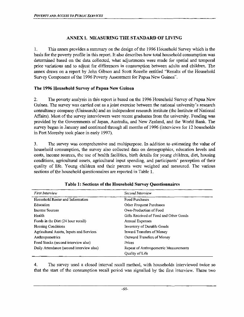
POVERTYAVD ACCESS TO PUBLICSER VICES
ANNEX I. MEASURING THE STANDARD OF LIVING
1. This annex provides a summary on the design of the 1996 Household Survey which is thebasis for the poverty profile in this report. It also describes how total household consumption wasdetermined based on the data collected, what adjustments were made for spatial and temporalprice variations and to adjust for differences in consumption between adults and children. Theannex draws on a report by John Gibson and Scott Rozelle entitled "Results of the HouseholdSurvey Component of the 1996 Poverty Assessment for Papua New Guinea".
The 1996 Household Survey of Papua New Guinea
2. The poverty analysis in this report is based on the 1996 Household Survey of Papua NewGuinea. The survey was carried out as a joint exercise between the national university's researchconsultancy company (Unisearch) and an independent research institute (the Institute of NationalAffairs). Most of the survey interviewers were recent graduates from the university. Funding wasprovided by the Governments of Japan, Australia, and New Zealand, and the World Bank. Thesurvey began in January and continued through all months of 1996 (interviews for 12 householdsin Port Moresby took place in early 1997).
3. The survey was comprehensive and multipurpose. In addition to estimating the value ofhousehold consumption, the survey also collected data on demographics, education levels andcosts, income sources, the use of health facilities, birth details for young children, diet, housingconditions, agricultural assets, agricultural input spending, and participants' perception of theirquality of life. Young children and their parents were weighed and measured. The varioussections of the household questionnaires are reported in Table 1.
Table 1: Sections of the Household Survey Questionnaires
First Interview Second Interview
Household Roster and Information Food PurchasesEducation Other Frequent PurchasesIncome Sources Own-Production of FoodHealth Gifts Received of Food and Other GoodsFoods in the Diet (24 hour recall) Annual ExpensesHousing Conditions Inventory of Durable GoodsAgricultural Assets, Inputs and Services Inward Transfers of MoneyAnthropometrics Outward Transfers of MoneyFood Stocks (second interview also) PricesDaily Attendance (second interview also) Repeat of Anthropometric Measurements
Quality of Life
4. The survey used a closed interval recall method, with households interviewed twice sothat the start of the consumption recall period was signalled by the first interview. These two
-60-

POVERTYAND ACCESS TO PUBLICSERVICES
interviews were designed to be two weeks apart, which is the usual length of the pay period inPapua New Guinea. Data were collected on all food consumption (36 categories) and otherfrequent expenditures (20 categories) during the recall period. An unbounded recall covered31 categories of annual expenses, and an inventory of 16 durable assets collected informationneeded to estimate the value of the flow of services.
5. In addition to the household interviews, a community questionnaire was used to collectinformation on access to education, health, transport and communication services. Price surveyswere also carried out, with prices collected for 35 items.
Sample Design
6. Sample selection was based on a stratified two-stage random sample design. The 1990Census of Population provided the area sampling frame. The sample was divided into two mainstrata: (i) the National Capital District (NCD), and (ii) all other areas of the country (excludingNorth Solomons province where the Bougainville crisis prevented surveying, and in fact had alsoprevented the 1990 Census). The sample was designed so that 240 households (one-fifth) wouldcome from the NCD, and 960 households would come from the rest of the country. The mainreason for this stratification was to allow different sampling fractions, with a five times heaviersampling rate in the NCD. This heavier sampling was designed to create a big enough sample inthe NCD to allow comparison of poverty rates in 1996 and 1985-87; the estimates of poverty forthe earlier period coming from the Urban Household Survey. The different sampling fractions forthe two strata are controlled for by using weights (expansion factors) when forming nationalestimates.
7. A further stratification was applied to the non-NCD sample, mainly to improve theprecision of sample estimates. All primary sampling units ("Census Units") were divided intoone of 18 strata, based on three attributes: elevation, rainfall, and a proxy for "economicaccessibility". Elevation was chosen because results from the 1982-83 National Nutrition Survey(NNS) suggest that malnutrition of young children is greatest in the highlands fringe zone ofelevation 600-1200m. Only a small proportion (six percent) of the national population lives inthis elevation range, so stratification and systematic sampling (selection at a fixed interval with arandom start) was chosen to ensure that the right proportion of sampled households came fromthe highlands fringe. Rainfall was chosen because households in low rainfall areas may havemore variable consumption patterns over the course of a year. Even within the same elevationand rainfall class, there is great variability, so "economic accessibility" was used as the thirdstratifying variable, to ensure the right proportion of both remote and accessible villages in thesample.
8. The proxy for "economic accessibility" was based on data from two sources. The firstwas estimates of mean cash income per household from agricultural activities, for the"agricultural system" in which the Census Unit is located. This came from a national agriculturalmapping project. The second was estimates of the proportion of households who ate rice the
-61-
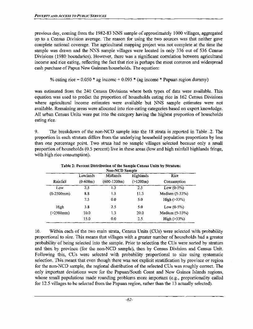
POVERTYANDACCESS To PUBLICSERVICES
previous day, coming from the 1982-83 NNS sample of approximately 1000 villages, aggregatedup to a Census Division average. The reason for using the two sources was that neither gavecomplete national coverage. The agricultural mapping project was not complete at the time thesample was drawn and the NNS sample villages were located in only 336 out of 536 CensusDivisions (1980 boundaries). However, there was a significant correlation between agriculturalincome and rice eating, reflecting the fact that rice is perhaps the most common and widespreadcash purchase of Papua New Guinean households. The equation:
% eating rice = 0.050 * ag income + 0.095 * (ag income * Papuan region dummy)
was estimated from the 240 Census Divisions where both types of data were available. Thisequation was used to predict the proportion of households eating rice in 162 Census Divisionswhere agricultural income estimates were available but NNS sample estimates were notavailable. Remaining areas were allocated into rice-eating categories based on expert knowledge.All urban Census Units were put into the category having the highest proportion of householdseating rice.
9. The breakdown of the non-NCD sample into the 18 strata is reported in Table .2. Theproportion in each stratum differs from the underlying household population proportions by lessthan one percentage point. Two strata had no sample villages selected because only a smallproportion of households (0.5 percent) live in these areas (low and high rainfall highlands fringe,with high rice consumption).
Table 2: Percent Distribution of the Sample Census Units by Stratum:Non-NCD Sample
Lowlands Midlands Highlands Rice
Rainfall (0-600m) (600-1200m) (>1200m) Consumption
Low 2.5 1.3 2.5 Low (0-5%)
(0-2500mm) 8.8 1.3 11.3 Medium (5-33%)
7.5 0.0 5.0 High (>33%)
High 3.8 2.5 5.0 Low (0-5%)
(>2500mm) 10.0 1.3 20.0 Medium (5-33%)
15.0 0.0 2.5 High (>33%)
10. Within each of the two main strata, Census Units (CUs) were selected with probabilityproportional to size. This means that villages with a greater number of households had a greaterprobability of being selected into the sample. Prior to selection the CUs were sorted by stratumand then by province (for the non-NCD sample), then by Census Division and Census Unit.Following this, CUs were selected with probability proportional to size using systematicselection. This meant that even though there was not explicit stratification by province or regionfor the non-NCD sample, the regional distribution of the selected CUs was roughly correct. Theonly important deviations were for the Papuan/South Coast and New Guinea Islands regions,whose small populations made rounding problems more important (e.g., proportionality calledfor 12.5 villages to be selected from the Papuan region, rather than the 13 actually selected).
-62-

POVERTYA,VDACCESS To PuBLiC SER ViCES
11. A subset of one-sixth of the selected CUs were chosen as a longitudinal sub-sample.Households were interviewed in these CUs at two different times of the year, roughly eightmonths apart, so that the correlation between expenditures in different months of the year for thesame household could be measured. This correlation is needed for unbiased estimation of thebetween-households variance of annual expenditures when the data come from short periodrecall expenditures. The usual method of calculating the variance of annual expenditures, whichis based on extrapolating annual expenditure from short period recall data, overstates the truevariance. This can bias estimates of the incidence of poverty because the overstated varianceincreases the proportion of households whose expenditures fall below a certain absolute cut-off,e.g., a poverty line.
12. The revisit interviews for the longitudinal sub-sample also provide an opportunity tomake the sample more representative of an entire year. The survey had initially been planned totake place only in the early months of 1996 because an October deadline had been set foravailability of the results, to coincide with preparations for the annual PNG Budget. Thisdeadline was subsequently relaxed after fieldwork had started but by then a greater number ofinterviews had been carried out in January and February than would have taken place ifinterviewing was spread evenly over the 12 months of the year. However, by using revisitinterviews, which took place from August onwards, to replace first visit interviews, the over-representation of January and February in the sample is reduced, and interviews are spread moreevenly over the year. This replacement is possible because the CUs to be revisited were chosenfrom a randomly selected group and the complete survey was repeated when the household wasrevisited. In fact, the interviews are possibly more accurate during the revisits than the initialvisits because of the greater experience of the interview teams.
13. At the second stage of sampling, households were randomly selected from within theselected CUs. Selection was based on a listing of all households within the Census Unit. Thislisting was carried out by the survey team just after arrival in each CU. A fixed number ofhouseholds were selected: six per Census Unit in the NCD sample, and 12 in the non-NCDsample. The reason for making this difference is that fieldwork costs (e.g., transportation) arelower in an urban area like the NCD, so the sampling efficiency advantages of a smaller clustersize outweigh the budgetary advantages of a larger cluster size. If the size of the CU, in terms of1990 census households reported, were always equal to the 1996 household count, the selectionof a fixed number of households in every CU would lead to a self-weighting sample. In practicethough, these two numbers are likely to differ in most CUs, whether due to error in the census,error in the household count, or real population change. Thus self-weighting cannot be assumedand weights will be needed. See below.
14. A set of "reserve" households were also selected from the household listing in each CU,by the same method that was used to select the initial sample. These reserve households wereused if any of the originally selected ones were unavailable or were unwilling to co-operate withthe survey. Reserves were used only for households that were unavailable for the first interview.If the first interview was completed for a particular household but that household then became
-63-
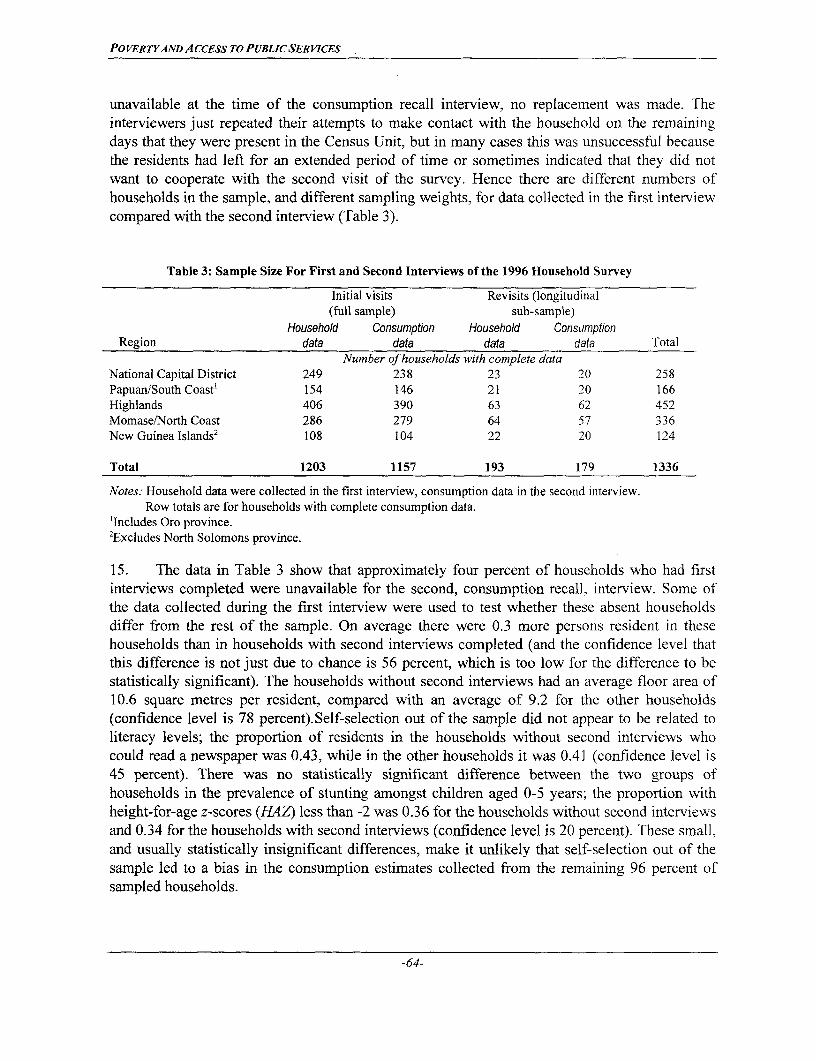
POVERTYANDACCESS To PUBLIC SER VICES
unavailable at the time of the consumption recall interview, no replacement was made. Theinterviewers just repeated their attempts to make contact with the household on the remainingdays that they were present in the Census Unit, but in many cases this was unsuccessful becausethe residents had left for an extended period of time or sometimes indicated that they did notwant to cooperate with the second visit of the survey. Hence there are different numbers ofhouseholds in the sample, and different sampling weights, for data collected in the first interviewcompared with the second interview (Table 3).
Table 3: Sample Size For First and Second Interviews of the 1996 Household Survey
Initial visits Revisits (longitudinal(full sample) sub-sample)
Household Consumption Household ConsumptionRegion data data data data Total
Number of households with complete dataNational Capital District 249 238 23 20 258Papuan/South Coast' 154 146 21 20 166Highlands 406 390 63 62 452Momase/North Coast 286 279 64 57 336New Guinea Islands2 108 104 22 20 124
Total 1203 1157 193 179 1336
Notes: Household data were collected in the first interview, consumption data in the second interview.Row totals are for households with complete consumption data.
'Includes Oro province.2Excludes North Solomons province.
15. The data in Table 3 show that approximately four percent of households who had firstinterviews completed were unavailable for the second, consumption recall, interview. Some ofthe data collected during the first interview were used to test whether these absent householdsdiffer from the rest of the sample. On average there were 0.3 more persons resident in thesehouseholds than in households with second interviews completed (and the confidence level thatthis difference is not just due to chance is 56 percent, which is too low for the difference to bestatistically significant). The households without second interviews had an average floor area of10.6 square metres per resident, compared with an average of 9.2 for the other households(confidence level is 78 percent).Self-selection out of the sample did not appear to be related toliteracy levels; the proportion of residents in the households without second interviews whocould read a newspaper was 0.43, while in the other households it was 0.41 (confidence level is45 percent). There was no statistically significant difference between the two groups ofhouseholds in the prevalence of stunting amongst children aged 0-5 years; the proportion withheight-for-age z-scores (HAZ) less than -2 was 0.36 for the households without second interviewsand 0.34 for the households with second interviews (confidence level is 20 percent). These small,and usually statistically insignificant differences, make it unlikely that self-selection out of thesample led to a bias in the consumption estimates collected from the remaining 96 percent ofsampled households.
-64-
POVERTYAND A CCESS T0 PUBLIC SERVICES
16. The attrition of originally selected households was also apparent in the longitudinal sub-sample. Only 89 percent of the originally interviewed households in the 20 CUs of thelongitudinal sub-sample were able to be re-interviewed, approximately eight months after thefirst interviews. Some of this attrition reflected the mobility of households and some reflected anunwillingness to further participate. This unwillingness was due partly to an unmet demand formonetary compensation to replace the gifts that were given to participating households.
17. Three of the selected CUs in the non-NCD sample were too small to provide a sample of12 households. Two were combined with neighbouring Units and listing and household selectionwas carried out on the pseudo-Census Unit created from the joining of the two neighbouringUnits. The third. was in an area that was too remote and sparsely populated to allow a pseudo-Census Unit to be created, so only 11 households were selected in this instance. Five other non-NCD CUs had first and second interview data for only 11 households rather than the plannednumber of twelve. In some cases this arose because the number of households absent or refusingexceeded the number of reserve households provided; in two further cases questionnaires werelost after the interviews were completed. For all of these CUs, sampling weights for theremaining households are modified so that the CUs are not under-represented (the weight israised by a factor of 1.09=12/1 1).
18. The first cell in Table 3 shows that more households were surveyed in the NationalCapital District than the target of 240. The cause was the experiment of comparing diaries versusrecall (described below) which required three households in each CU to be surveyed by the diarymethod and three by the recall method. Some interviewers became confused and issued diaries toall six households, so a further three households had to be chosen from the reserve list for therecall sub-sample. Rather than waste the information provided by the 'excess' households, theyare included in the sample and the sampling weights are multiplied by a factor of 0.67 (=6/9) forhouseholds in the affected CUs.
19. The sample in the NCD was also distinguished by selecting some CUs in growth areasthat had not existed at the time of the 1990 Census. The National Statistical Office recognisedand mapped approximately 50 new CUs in the NCD, as part of their work for a Demographic andHealth Survey. Four of these new growth areas (two in settlements and two in formal housingschemes) were selected as part of the sample of 40 CUs, using the same fixed interval samplingas the rest of the NCD sample. In the non-NCD sample no attempt was made to identify, andseparately sample, new villages or new CUs not in the census. This does not necessarily implysignificant under-coverage: new household settlements may often create new hamlets which areautomatically absorbed in the nearest CU, or individual new households may be added to the CUsimply because boundaries are large and vague. In any case the selected CU is always subject toa pre-survey household count and this provides a population up-date which should in most casesbe complete.
20. Some rural CUs were too large to fully list. This was especially in rural areas of theHighlands, where the Census still operates by "line-up enumeration". Some of these CUs had
-65-

POVERTYAND ACCESS TO PUBLIC SER VICES
over 500 households and these households were not located in villages, but were scattered widelyin small hamlets over a considerable geographical area. Moreover, not every household living inthe same area lines up together at the Census because clan lineage and marriage rather thanphysical location of residency appears to determine where a person lines up for Censusenumeration. These large, spread-out CUs were partitioned into segments by survey teams in thefield before listing, usually following expert local advice, and the segment to list and selecthouseholds from was then randomly picked. In some cases, a separate household listing wascarried out for the whole Census Unit, after the main survey had finished in December, to getmore accurate estimates of the sampling rate in terms of household numbers, which is needed forthe sampling weights (discussed below).
21. Surveying was not possible in six of the selected CUs, due to problems of tribal fighting,religious beliefs, and refusal of some communities to accept the survey. These six CUs and thereplacements that were selected for them are listed in Table 4. The usual method of replacementwas to form a list of CUs in the same province and stratum as the original Census Unit, and thenmake a random selection from that list, with probability proportional to size (1990 householdnumbers). In the case of Juguna, in the Baiyer area of Western Highlands, the replacementchosen by this method had itself to be replaced (by Aviamp) because of tribal fighting. Thereplacement made for Bitokara in West New Britain was done by the survey organiser in thefield using expert local knowledge to try to recreate the attributes of the original selection(distance to main towns, access to health and school facilities, extent of cash cropping). This wasachieved by combining a village with an adjacent mission (with school and health centre).
Table 4: Sample Replacements for the Non-NCD Sample
Census Replacement CU Census Reason forProvince Original CU Count Count Replacement
Oro Tiare 31 Nindewari 33 Religious beliefsEnga Yagonda 193 Papiyuku 264 Tribal fightingWestern Highlands Juguna 61 Aviamp 269 Tribal fighting/cultsMorobe Bupu 19 Muanu 53 Community refusalWest New Britain Tiaruru 232 Sarakolok 323 Oil palm disputeWest New Britain Bitokara 180 Gavuvu and 53 Land dispute
Malalia mission
Sampling Weights
* A set of weights, which potentially can vary for each Census Unit in the sample, are neededwhen estimating statistics from the household data. These weights are needed to correct forthe varying selection probabilities of areas and households in different parts of the sample.They can be regarded as made up of three components:
* Correction for the differing sampling rates used in the strata at the area stage of sampling.This affects the two principal strata NCD and non-NCD. In addition, since areas are selectedwith probability proportional to "size", the size variable (census households reported) has to
-66-
POVERTYANDACCESS ToPUBLICSkRVICES
be included in the weighting. Essentially the weights here are obtained as the samplinginterval divided by the census size variable.
* Correction for varying numbers of households selected in the CU. This is made up of twocomponents: (1) the planned variation between 6 (in NCD) or 12 (in non-NCD), and (2) non-response, when the number of interviewed households within the CU differs from the desirednumber ( 6 or 12). These selected households have to be blown up to the number existing, ineach CU, that is to the number listed during the household listing operation. The weight ineach CU is the ratio of the number listed to the number interviewed. Separate weights areneeded for the first visit (household data) and the second visit (consumption data).
* A third weight is introduced in a few special cases, namely where the CU is subdivided intosegments. If si is the number of segments created in the i-th CU, and one of these is selectedat random, and if the listing covers only the selected segment, the weight must be si , thelisting total Mi' being the segment listing total. However, if the household listing isextended to cover the whole CU with a CU listing total of M*", then the weight should beMj"/Mi'. In the latter case the Mi' in the preceding term will of course cancel the Mi' in thefinal term.
22. Summarising, the weights to use for each Census Unit are given by the formula:
Whi =[ lh / bhi I . I Mhi'/ Mhi I
where the main strata (NCD and non-NCD) are indexed by h and Census Units by i, andIh is the interval used in the first stage sampling to select CUs (given by the ratio of the
number of households in that strata of the sampling frame to the number of CUs selected)bhi is the number of households interviewed in the Census Unit (where this can vary between
first interviews (household data) and second interviews (consumption data))Mhi is the number of households in the CU recorded at the 1990 Census (and this number, in
conjunction with the interval 'h and the systematic ordering of the CUs, lead to theselection of the particular Census Unit into the sample)
Mhi'is the number of households listed in the Census Unit or segment in 1996 (and thisdetermines the selection probability of any given household in the CU).
23. The sample of CUs for the National Capital District was drawn from two samplingframes that were put together. The first sampling frame was the 1990 census, which had 468CUs. The second frame was 50 new CUs that had been recently recognised (and mapped) by theNSO as part of the work requirements for the DHS. A systematic sample of 40 CUs was drawnfrom this combined frame.
24. The count of households done in 1996 by the interview teams was often substantiallydifferent from the 1990 Census count, ranging from being over four times larger, to being onlyone-quarter as large. Many of the CUs with apparently large changes in household numbers werein the Highlands, where the 1990 Census operated by 'line-up' enumeration. To ensure that the
-67-

POVERTYAND ACCESS TO PUBLICSERVICES
apparent size changes were not caused by the method of splitting Census Units into segments,return visits were made to completely list several of the large Highlands CUs. The locationswhere this re-listing was carried out are noted in Table 1.
25. Even after re-listing, several CUs with apparently large shifts in household numbers, andtherefore potentially large or small weights, remained in the sample. Some of the apparentdeclines in household numbers were able to be explained by factors such as people moving out ofareas with severe tribal fighting or crime problems (e.g., a 70 percent decrease in Buk in WesternHighlands). However, some of the instances of apparently rapid population growth seem moreeasily explained as errors of undercoverage in the 1990 Census (Table 5). In five of the six CUsthat appear to have household numbers double between 1990 and 1996, the 1990 count ofhouseholds was lower than the 1980 count, by a substantial amount in Won'em'men'ya (EHP),Wariman (ESP) and Kailge (WHP). It is only Erave Station (SHP) where the rapid growthbetween 1990 and 1996 is consistent with earlier growth rates.
Table 5: Census Units With Apparently Rapid Growth in Household Numbers
Estimates of Household Numbers Annual Growth Rates1980 1990 1996 1990-96 1980-96
Won'em'men'ya (EHP) 28 13 56 0.243 0.043Wariman (ESP) 64a 25 61 0.149 -0.003Baisarik (Madang) 30 26 61 0.142 0.044Semin (SHP) 170 165 380 0.139 0.050Kailge (WIHP) 161 91 211 0.140 0.017Erave St. (SHIP) 45 93 204 0.131 0.094
aBased on population, converted into household numbers assuming same average household size as found for theCensus Unit in 1990.
26. Although the aim was to select CUs with probability proportional to size, there is noassumption that the measures of size M, are accurate. If they are, the sampling (random) error islikely to be smaller, which is an advantage, but whether they are accurate or not there will be nobias, provided the above weights are used. Therefore the inaccuracy of the 1990 census is not acause for serious concern. Statisticians refer to the method used here as "probability proportionalto estimated size" and it is just as "respectable" as the more ideal case of true PPS. Above all itis important not to try to "correct" the values M, after the sample has been used. The value M;which appears in the denominator of the weighting formula is introduced in order to cancel thevarying probabilities which were used in selecting the CUs. This cancelling will only occur ifwe use identically the same values Mi in the weighting formula as were used in selecting thesample. That the size measures are inaccurate does not matter because they are going to beupdated by introducing the values Mi', coming from the very latest count.
Sampling Errors
27. Any estimates of averages, totals or ratios that are made from these survey data aresubject to sampling error because the estimates come from a sample rather than the full
-68-

POVERTYANDACCESS TO PUBLiCSERViCES
population of households in Papua New Guinea. The extent of sampling error is usuallymeasured by the "standard error", with smaller standard errors indicating that the estimate fromthe survey is more precise. In calculating the standard errors, allowance must be made for thetwo-stage sampling, where the selection of the 120 CUs was the first stage, and the selection ofhouseholds within these CUs was the second stage. This two-stage sampling is less efficient thansimple random sampling in statistical terms (i.e., causes larger standard errors). This is becausethe households within a CU tend to have similar characteristics, so a sample drawn from themreflects less of the population's diversity than would a simple random sample with the samenumber of households. Therefore, if methods appropriate for calculating standard errors from asimple random sample are used, the standard errors that are reported will underestimate the truemagnitude of sampling error.
28. The CENVAR software package, produced by the US Census Bureau, was used forcalculating standard errors. This package is based on PC CARP (Cluster Analysis andRegression Package) software, and uses the ultimate clusters sampling model for calculatingstandard errors from complex survey designs with the algorithm based on Taylor seriesapproximation (or "linearization"). Full details are available in the CENVAR documentation.
Measuring the Value of Household Consumption
29. Five components of household consumption were measured by the survey: foodconsumption; other frequent expenses; annual expenses; consumption of non-housing durables;and consumption of housing services. The main components of consumption that were notmeasured are consumption of leisure, consumption of environmental services, and consumptionof freely provided (or subsidised) public services. These items were excluded because of theconceptual and practical difficulties in measuring them.
30. The reference period for food consumption and other frequent purchases was set by thetime between the first and second interviews. This bounded period between the two interviewswas designed to be two weeks, but often differed from this, so the dates of each interview wererecorded. The reference period for annual expenses was the past 12 months. The estimates oftotal consumption are made on an annual basis by extrapolating food consumption and otherfrequent expenses from the bounded recall period up to a full year. The inter-household varianceof these estimates of annual consumption will be greater than if consumption was continuouslymeasured over a full 12 month period because some of the shocks that occur in the shortreference period would be evened out over the course of a year. The extent of this upward bias inthe measures of dispersion is discussed in the sensitivity analyses, using results from thelongitudinal sub-sample.
31. One problem in extrapolating short-term consumption from the bounded recall referenceperiod, and then adding it to annual expenses, is that the size of the household may differbetween the short and the long time periods. For example, a household may usually have fiveresidents but during the bounded recall period two members leave to visit friends in anotherhousehold for six days. This will cause the consumption of food and other short-term expenses tofall and when this is extrapolated to the full year it will lower the estimated annual value of the
-69-
POVERTY AND ACCESS TO PUBLIC SERVICES
household's consumption. If total annual consumption was divided by the number of usualresidents (five), the result would understate the true level of per capita consumption, because forthe rest of the year the two people who were absent during part of the recall period are living inthe household and contributing to its consumption. Therefore some adjustment needs to be madefor the effect of absent residents, and for the opposite effect of short-term guests (and thesecorrections need to offset so that there is no double counting).
32. The specific adjustment used was as follows: the potential number of person-days duringthe recall period was estimated as the number of calendar days between the two interviewsmultiplied by the number of persons listed in the household roster. The actual number of person-days was measured from a schedule of absences and guests (present for at least seven days). Anallowance was made for the smaller impact of absent or additional young children by estimatingperson-days in adult-equivalent terms, where each child aged six and below had a weight of 0.5(see below for evidence on this equivalence scale). The ratio of the actual number of person-daysto the potential number was formed and used to estimate the annualized equivalent of thebounded recall period consumption as:
365 Potential days(Food + Other Frequent Expenses) x x
(Bounded Period) Actual days
33. If someone was listed as a usual resident on the roster but was substantially absent duringthe bounded recall period (absent at least 10 days), they were not counted when estimatinghousehold size, and therefore the above correction factor for absences was not applied to get theannual estimate of the recall period consumption. An exception to this rule was children whowere away at school during the bounded recall period but whose school fees and other costs arestill being met by the household. These children were considered to be part of the household andthey therefore counted when estimating household size.
Food Consumption34. Food consumption was measured by a residual approach using the equation:
Purchases+ Own-production+ Gifts received- Sales- Gifts given- Stock increases
= Consumption.
35. This approach was chosen for two reasons. First, it was the method that had been usedpreviously in PNG in the Urban Household Survey and the Household Expenditure Survey.Second, there is substantial interest in some of the components of consumption in their ownright, especially the quantity and value of domestic food production and sales.
-70-

POVERTYAND ACCESS TO PUBLICSERVICES
36. The inclusion of sales of items that were either self-produced or purchased is animportant part of the fornula for calculating consumption. Previous evidence from urban areasshows that ignoring this can substantially overstate the consumption of items like beer that arebought to be then resold on the black market, and also overstates the consumption of foods wherea substantial amount of production is sold, e.g., betel nut. The importance of small-scale sellingactivity might be overstated if the purchases and sales of more formal business entities, like tradestores, were recorded as household transactions. Therefore, food purchases that were expenses ofa formal business were ignored, as were the corresponding sales by these same household-business units. However, the expenses of an informal business, like flour purchases by a sconeseller, were counted as food purchases, and sales (valued at input costs) were then subtracted togive the estimate of consumption.
37. The residual approach to measuring consumption does suffer some drawbacks. If formsof food disappearance that are not included in the formula -- such as plate waste and feedinghousehold food to domestic animals -- are important, apparent food consumption levels will beoverstated. The residual approach is also less intuitive than directly asking households what theyeat, and there is international evidence that estimates of calorie intake based on what householdseat are less extreme (higher for poor households and lower for rich households) than aremeasures of calorie availability based on an expenditure approach. Because the residual approachdepends on six separate components there is also more scope for error. For example, havinghigher stocks of a food at the end of the recall period than at the start, but no record of purchases,production or gifts received to account for the higher stocks, could be due to error in any one offour possible parts of the interview.
38. The most difficult part of the food consumption equation to obtain reliable measures ofwas food production. Locally produced foods, which include root crops, bananas, vegetables andsago, are not sold by weight in Papua New Guinea. Instead, they are sold in fixed price bunches,bundles, heaps, or piles. Although some rural people are familiar with kilogram weights fromsales of coffee or purchases of flour, rice or stock food, the densities of these items are muchdifferent to the densities of root crops. A further difficulty is the high volume of production, dueto the bulky nature of the local staples (excluding sago); an average sized rural household caneasily produce over 100 kg of root crops per week. In these circumstances it was consideredunwise to ask respondents: "how many kilograms of food x did your household produce since mylast visit?" Such answers reported in kilogram units would give the appearance of accuracy butthis would just disguise the problem of measuring food production and force it onto theinterviewers and the respondents.
39. Instead of relying exclusively on kilogram units, the question on food production allowedflexibility in the choice of units. Five units were available. The first was an empty 25 kg rice bag,which had three graduations ("1/4", "21'", ""3/4) marked on the outside. This bag was given to thehousehold at the start of the survey and they were asked to put their produce into it during therecall period. This was the recommended unit for bulky crops. The other units were bunches andheaps; kilograms; singles, which were recommended for items like coconut and betelnut, and
-71-
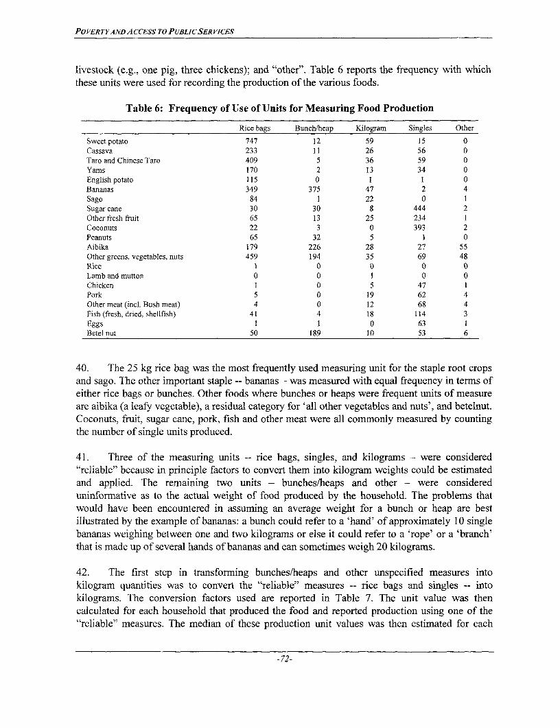
POVERTYAND ACCESS TO PUBLIC SER VICES
livestock (e.g., one pig, three chickens); and "other". Table 6 reports the frequency with whichthese units were used for recording the production of the various foods.
Table 6: Frequency of Use of Units for Measuring Food Production
Rice bags Bunch/heap Kilogram Singles Other
Sweet potato 747 12 59 15 0Cassava 233 11 26 56 0Taro and Chinese Taro 409 5 36 59 0Yams 170 2 13 34 0English potato 115 0 1 1 0Bananas 349 375 47 2 4Sago 84 1 22 0 1Sugar cane 30 30 8 444 2Other fresh fruit 65 13 25 234 1Coconuts 22 3 0 393 2Peanuts 65 32 5 1 0Aibika 179 226 28 27 55Other greens, vegetables, nuts 459 194 35 69 48Rice 1 0 0 0 0Lamb and mutton 0 0 1 0 0Chicken 1 0 5 47 1Pork 5 0 19 62 4Other meat (incl. Bush meat) 4 0 12 68 4Fish (fresh, dried, shellfish) 41 4 18 114 3Eggs I 1 0 63 1Bete] nut 50 189 10 53 6
40. The 25 kg rice bag was the most frequently used measuring unit for the staple root cropsand sago. The other important staple -- bananas - was measured with equal frequency in terms ofeither rice bags or bunches. Other foods where bunches or heaps were frequent units of measureare aibika (a leafy vegetable), a residual category for 'all other vegetables and nuts', and betelnut.Coconuts, fruit, sugar cane, pork, fish and other meat were all commonly measured by countingthe number of single units produced.
41. Three of the measuring units -- rice bags, singles, and kilograms - were considered"reliable" because in principle factors to convert them into kilogram weights could be estimatedand applied. The remaining two units - bunches/heaps and other - were considereduninformative as to the actual weight of food produced by the household. The problems thatwould have been encountered in assuming an average weight for a bunch or heap are bestillustrated by the example of bananas: a bunch could refer to a 'hand' of approximately 10 singlebananas weighing between one and two kilograms or else it could refer to a 'rope' or a 'branch'that is made up of several hands of bananas and can sometimes weigh 20 kilograms.
42. The first step in transforming bunches/heaps and other unspecified measures intokilogram quantities was to convert the "reliable" measures -- rice bags and singles -- intokilograms. The conversion factors used are reported in Table 7. The unit value was thencalculated for each household that produced the food and reported production using one of the"reliable" measures. The median of these production unit values was then estimated for each
-72-
POVERTYANDACCESS To PUBLICSERVICES
food in every Census Unit in the non-NCD sample, with the exception of meat and fish, wherethe median was calculated over all households in the region. The final step in imputing kilograrnquantities was to take the monetary value that households had assigned to the particular food thatwas measured with an uninformative quantity unit, and divide that value by the median unitvalue. If no median unit value had been calculated for that Census Unit - either because no otherhouseholds produced the food or because the quantity measurement for all households whoproduced the food was an uninformative one - the imputation was based on the median unitvalue from the full sample of households in all non-NCD Census Units. In the NCD sample, themonetary values assigned to production of foods with uninformative quantity units were dividedby market prices, in order to impute the quantity of production in kilograms.
43. The distinction made above between "reliable" and uninformative quantity units isblurred somewhat by the imprecision of the conversion factors estimated for rice bags andsingles. The three foods having the largest number of measurements of both weight and rice bagswere sweet potato, taro and bananas. The coefficient of variation (standard deviation relative tothe mean) of the weight of a rice bag full of each of these foods was estimated as 0.3, 0.2, and0.2. A further imprecision is that the relationship between how full the rice bag was and theweight is not linear. Instead a full bag would contain roughly one kilogram more than two halffull bags, but the survey form just records the total number of bags produced and not whetherthat total is made up of very many fractions of bags or just a few full bags. The situation is evenworse for the variability in the weight of single items: the average weight of a single sweet potatoassumed by the unit value (and calorie) calculations was 0.45 kg, but weights found during thesurvey ranged from 2.5 kg to 0.1 kg. The estimated coefficients of variation for single sweetpotato and cassava were 0.9, for taro 1.0, for yam 1.4, and for banana (single 'fingers') 0.7. Evenitems where individual units have a relatively regular size, like coconuts and betelnuts, hadestimated coefficients of variation of about 0.4. The problems are bigger when assigning anaverage weight to an individual animal such as a pig, because whole pigs were not able to beweighed during the course of the survey. For items that are aggregations or residual categories(e.g., "other fresh fruit", "other greens, vegetables, and nuts") the average weight used for bothrice bags and singles will be a very noisy measure of the actual weight of production of anyparticular household because we don't know if, for example, the item produced is a pineapple,whose average weight is about 2 kg, or a mango, whose average weight is just 0.3 kg.
44. The imprecision of the conversion factors in Table 7 means that for any given household,the estimated quantity of food production will contain a substantial element of random noise. Ifthis noise increases the measured between-household dispersion, the number of householdsbelow a poverty line might be overstated. But sample summary statistics such as means and totalshould not be affected if the conversion factors are right, on average. This also applies to anymeasures derived from food quantities, such as per capita calorie availability.
-73-

POVERTY AND ACCESS TO PUBLIC SERVICES
Table 7: Weight Conversion Factors Used for Measuring Food Production
---------- Kilograms per ---
25 kg rice bag Single Bunch/heap/other
Sweet potato 19 0.45 2.0Cassava 16 0.7 1.5Taro and Chinese Taro 16 0.6 1.8Yams 16 0.7 1.4English potato 20 0.1 0.6Bananas 12 0.16 1.6Sago 30 n.a. 1.0Sugar cane 20 2.5 5.0Other fresh fruit 12 0.8 1.0Coconuts 18 1.3 2.6Peanuts 8 0.01 0.2Aibika 4 0.06 0.2Other greens, vegetables, nuts 10 0.4 1.0Rice 20 n.a. 1.0Lamb and mutton 15 20 n.a.Chicken 15 1.5 n.a.Pork 15 30 n.a.Other meat (incl. bush meat) 15 3.0 n.a.Fish (fresh, dried, shellfish) 15 0.5 1.0Eggs 15 0.06 0.5Betel nut 19 0.03 0.15
45. Although considered an uninformative unit of measure, there was one circumstance whenweights had to be assumed for bunches/heaps and "others". This occurred when a householdeither gave away or sold food that it had produced, and the gift or sale was measured in units ofbunches or heaps, while the original production had been measured in another unit. The finalcolumn of Table 7 contains the conversion factors that were assumed for this purpose. Thisshould not cause large errors because the most common way of reporting gifts and sales was inthe same units as production was reported, which made calculating the fraction given or soldeasy, regardless of whether production was recorded using uninformative quantity units.
46. The computer programs that calculated food consumption used the median productionunit value in three other ways, additional to converting uninformative quantity units intokilograms. These uses were:
* Imputing the quantity of gifts received and the quantity of purchases, from the value ofgifts received and value of purchases, if the quantities had not been recorded.Although in principle, a Census Unit median could be calculated for purchase unitvalues and gift unit values, for the locally produced foods there was much moreinformation on production than on gifts received or purchases.
* Assigning a value to beginning food stocks, if the household reported no production,purchases or gifts received of the food concerned. Usually there would be either
-74-
POJVERTYANDACCESS TO PUBLIC SERVICES
production or purchases or gifts received, so the ratio of sub-total values and quantitiescould be used to implicitly give food stock changes the same household-specific unitvalue as was applied to production, purchases and gifts.
Creating an alternative measure of the value of each household's production of eachfood, by multiplying the household's production quantity by the Census Unit medianof the production unit value for that food. This alternative measure can only be createdif "reliable" quantity units were used.
47. For all three of these uses, the regional average market price was used for foods that arenot produced in PNG (including rice and sheepmeat, whose local production is almost zero). Forthe food consumption of households in the NCD sample, the average market price was used forall foods instead of the median production unit value.
48. Using the median unit value to adjust the value of production is appropriate if (i) it isassumed that the law of one price holds within CUs, and (ii) it is believed that quantitiesmeasured with "reliable" units are more accurate than reports of how much it would cost to buyor sell the quantity of a certain food produced by the household. The reason for doubting thereports of values is that very few households who are producing a food also buy that same food,so there may be a lot of misinformation about prices. Sales activity is also low so manyhouseholds would not be able to infer purchase values from the prices they receive when sellingthe food. In these circumstances there may be a lot of random noise in the values attributed toself-produced foods.
49. The unit values for production of sweet potato were examined to see how important thisrandom noise in the values attributed to self-produced foods may be. Attention was restrictedjust to households who used the 25 kg rice bag as the unit of measure and just to CUs where unitvalues for the rice bag were available for at least four households (n=694). The within CensusUnit coefficient of variation in the value that each household placed on a rice bag full of self-produced sweet potato was 0.45, which is twice as high as the variation in the measured weightof rice bags of sweet potato. These households were ranked within their CUs, according to thevalue they placed on a rice bag of sweet potato. The ratio of the highest unit value to the lowestunit value was formed, and the median value of this ratio was estimated to be four. Hence, thereappears to be large variation in the value that households within the same Census Unit placed ona given volume of production. Some of this variation will be caused by the differing weight ofsweet potato that each household's rice bag contained, but this source cannot explain it all. Somemore of the variation may be due to differences in the quality of sweet potato that eachhousehold was producing. However, at least some of the remaining variation would seem to bedue to differences in opinions about prices.
50. The variation in sweet potato unit values found within CUs is likely to occur with otherself-produced foods as well. It may seem unreasonable that two households, who produce thesame quantity of a food in the same location, can have that production valued differently. Ahousehold might fall below the poverty line just by being too pessimistic when valuing their ownfood production because they think prices are lower than they truly are. Using the adjusted values
-75-
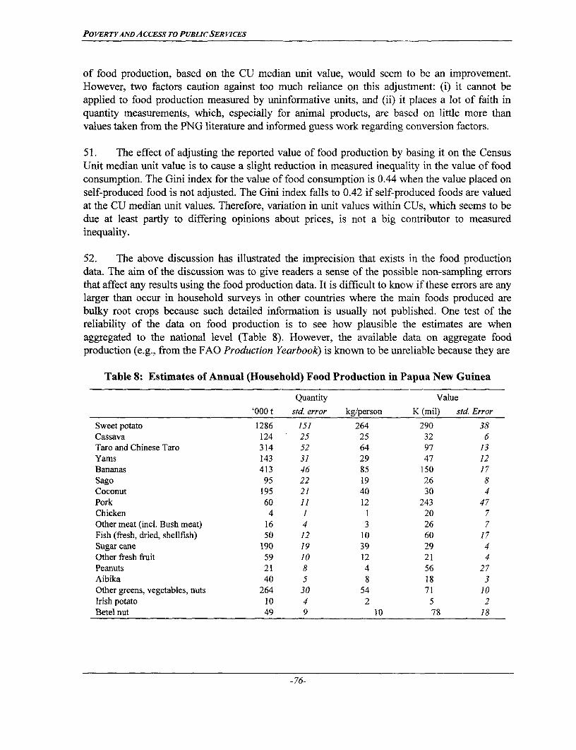
POVERTYANDACCESS To PUBLICSERVICES
of food production, based on the CU median unit value, would seem to be an improvement.However, two factors caution against too much reliance on this adjustment: (i) it cannot beapplied to food production measured by uninformative units, and (ii) it places a lot of faith inquantity measurements, which, especially for animal products, are based on little more thanvalues taken from the PNG literature and informed guess work regarding conversion factors.
51. The effect of adjusting the reported value of food production by basing it on the CensusUnit median unit value is to cause a slight reduction in measured inequality in the value of foodconsumption. The Gini index for the value of food consumption is 0.44 when the value placed onself-produced food is not adjusted. The Gini index falls to 0.42 if self-produced foods are valuedat the CU median unit values. Therefore, variation in unit values within CUs, which seems to bedue at least partly to differing opinions about prices, is not a big contributor to measuredinequality.
52. The above discussion has illustrated the imprecision that exists in the food productiondata. The aim of the discussion was to give readers a sense of the possible non-sampling errorsthat affect any results using the food production data. It is difficult to know if these errors are anylarger than occur in household surveys in other countries where the main foods produced arebulky root crops because such detailed information is usually not published. One test of thereliability of the data on food production is to see how plausible the estimates are whenaggregated to the national level (Table 8). However, the available data on aggregate foodproduction (e.g., from the FAO Production Yearbook) is known to be unreliable because they are
Table 8: Estimates of Annual (Household) Food Production in Papua New Guinea
Quantity Value
'000 t std. error kg/person K (mil) std. Error
Sweet potato 1286 151 264 290 38Cassava 124 25 25 32 6Taro and Chinese Taro 314 52 64 97 13Yams 143 31 29 47 12Bananas 413 46 85 150 17Sago 95 22 19 26 8Coconut 195 21 40 30 4Pork 60 11 12 243 47Chicken 4 1 1 20 7Other meat (incl. Bush meat) 16 4 3 26 7Fish (fresh, dried, shellfish) 50 12 10 60 17Sugar cane 190 19 39 29 4Other fresh fruit 59 10 12 21 4Peanuts 21 8 4 56 27Aibika 40 5 8 18 3Other greens, vegetables, nuts 264 30 54 71 10Irish potato 10 4 2 5 2Betel nut 49 9 10 78 18
-76-

POVERTYAND ACCESS TO PUBLIC SER VIcES
simply extrapolations from the 1961-62 Survey of Indigenous Agriculture (the standard errors forthis survey were over 25 percent. A stronger test of the plausibility of the current estimates willcome when final results are available from the national agricultural mapping project.
53. The dominance of sweet potato in local food production is evident from Table 8. Thequantity of sweet potato production is three times higher than the next highest food, bananas, andit is also the most valuable food crop. The other important foods in terms of quantity are taro andChinese taro (which in a mistaken decision early in the survey planning were combined as onerecall item to shorten the list of foods), coconut, sugar cane, yams, cassava, and the residualcategory of vegetables. In terms of value, pig production was second to sweet potato, followedby bananas, taro and Chinese taro, and betelnut. The aggregate value of food production wasapproximately K1.3 billion (standard error of KI 14 million). If the value of firewood andtobacco production was included, the total value of household production would be almost K1.6billion per year.
Other Frequent Expenses
54. Measuring consumption of non-food frequent expenses (e.g., gambling, P.M.V. fares,kerosene, tobacco) was easier than measuring food consumption because, with the exception ofleaf tobacco and firewood, consumption was entirely from purchases and gifts, rather than fromown-production. The other simplification was that quantities were not required.
55. The only problem encountered was assigning values to firewood, because in some areasfirewood is not bought and sold, so respondents had difficulty assigning a value to the firewoodthey harvested or received as gifts. A regression equation was used to impute firewood values ifthey were missing, using three assumptions to guide the specification of the equation. Morefirewood, and hence a higher value, is needed if:
* there is more food to be cooked,
* there are more people in the household to cook for and keep warm, and
* the outside temperature is colder.
The equation used was:Firewood Value = 39.1 (Number in household)
(4.0)+ 0.017 (Value of Food Purchased & Produced)
(2.8)+ 61.5 (Number in household * Highlands dummy)(4.6)+ 0.027 (Value of Food * Highlands dummy)
(4.0)N=821 R2z=0.30 (t-statistics).
-77-
POVERTYAND ACCESS TO PUBLICSERVICES
Annual Expenses
56. Annual expenses were estimated from an unbounded 12 month recall, with consumptionderived from three components:
Value of Purchases - Value of Gifts Given + Value of Gifts Received.
Spending on some of the items on the annual expenses schedule was also recorded in somesections of the first interview questionnaire (e.g., school fees, charges for water) and these datawere used to check the consistency of results. Any purchases of an item on the annual expensesschedule during the bounded recall period were also recorded, and these short-term data wereused to assess the consistency of the reported values given in the long term recall.
57. One of the categories of annual expense items that had data collected - loan paymentsand finance fees -- is not included in measured consumption. Many of the data reported for thiscategory appeared to be for repayments of principle as well as payments of interest. Theappropriate component for measuring consumption is just the interest payment because this is thecost to the household of bringing forward in time the acquisition of assets. If principalrepayments were included, measured consumption would have been overstated.
58. Two other notable items of the annual expenses are spending on bride price ceremonies,and spending on death feasts. Consumption of these two items was defined in the conventionalway, so for example, contributing to the bride price expenses of someone who lives outside thehousehold subtracts from the household's measured consumption. It could be argued that inPapua New Guinea contributing to the bride price and death feast expenses of kinsmen is arequirement of participating in the everyday life of the community. Hence, these expenses onpeople living outside the household might be a legitimate component of consumption and of aconsumption-based poverty line (World Bank, 1990). However, that line of argument was notfollowed when constructing the annual expenses variable. Thus spending on bride priceceremonies and death feasts for people outside the household was treated in the same way asother items purchased and then given away as gifts, by subtracting it from the householdsmeasured consumption.
Consumption of Durables
59. An inventory of 16 durable assets was used to collect data on the purchase price (or valueif it was a gift) and date of acquisition of each asset, and the price that it would realize if sold.Purchase prices were inflated to 1996 terms using the movement in the Consumer Price Index.The straight-line annual depreciation was calculated as:
(Purchase Value - Estimated Sales Value) / (1996 - Year of Acquisition).
If components of the formula were missing, a default value of annual depreciation was assignedbased on the average depreciation for that asset calculated from the sample of households withcomplete data. Table 9 contains these default depreciation values along with estimates of theownership rates for each durable in each region and the country as a whole.
-78-
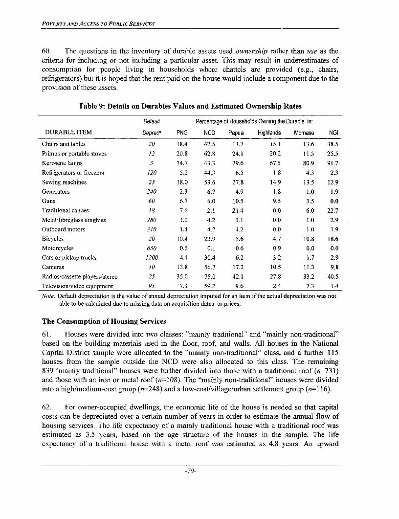
POVERTYANDACCESS TO PUBLICSERVICES
60. The questions in the inventory of durable assets used ownership rather than use as thecriteria for including or not including a particular asset. This may result in underestimates ofconsumption for people living in households where chattels are provided (e.g., chairs,refrigerators) but it is hoped that the rent paid on the house would include a component due to theprovision of these assets.
Table 9: Details on Durables Values and Estimated Ownership Rates
Default Percentage of Households Owning the Durable in:
DURABLE ITEM Deprecn PNG NCD Papua Highlands Momase NGI
Chairsandtables 20 18.4 47.5 13.7 15.1 13.6 38.5
Primus or portable stoves 12 20.8 62.8 24.1 20.2 11.5 25.5
Kerosene lamps 3 74.7 43.3 79.6 67.5 80.9 91.7
Refrigerators or freezers 120 5.2 44.3 6.5 1.8 4.3 2.3
Sewing machines 23 18.0 53.6 27.8 14.9 13.5 12.9
Generators 240 2.3 6.7 4.9 1.8 1.0 1.9
Guns 60 6.7 6.0 10.5 9.5 3.5 0.0
Traditional canoes 18 7.6 2.1 21.4 0.0 6.0 22.7
Metal/fibreglass dinghies 280 1.0 4.2 1.1 0.0 1.0 2.9
Outboard motors 310 1.4 4.7 4.2 0.0 1.0 1.9
Bicycles 20 10.4 22.9 15.6 4.7 10.8 18.6
Motorcycles 650 0.5 0.1 0.6 0.9 0.0 0.0
Cars or pickup trucks 1200 4.4 30.4 6.2 3.2 1.7 2.9
Cameras 10 13.8 56.7 17.2 10.5 11.3 9.8
Radios/cassette players/stereo 25 35.0 75.0 42.1 27.8 33.2 40.5
Television/video equipment 95 7.3 59.2 9.6 2.4 7.3 1.4
Note: Default depreciation is the value of annual depreciation imputed for an item if the actual depreciation was notable to be calculated due to missing data on acquisition dates or prices.
The Consumption of Housing Services
61. Houses were divided into two classes: "mainly traditional" and "mainly non-traditional"based on the building materials used in the floor, roof, and walls. All houses in the NationalCapital District sample were allocated to the "mainly non-traditional" class, and a further 115houses from the sample outside the NCD were also allocated to this class. The remaining839 "mainly traditional" houses were further divided into those with a traditional roof (n=731)and those with an iron or metal roof (n=108). The "mainly non-traditional" houses were dividedinto a high/medium-cost group (n-=248) and a low-cost/village/urban settlement group (n=1 16).
62. For owner-occupied dwellings, the economic life of the house is needed so that capitalcosts can be depreciated over a certain number of years in order to estimate the annual flow ofhousing services. The life expectancy of a mainly traditional house with a traditional roof wasestimated as 3.5 years, based on the age structure of the houses in the sample. The lifeexpectancy of a traditional house with a metal roof was estimated as 4.8 years. An upward
-79-
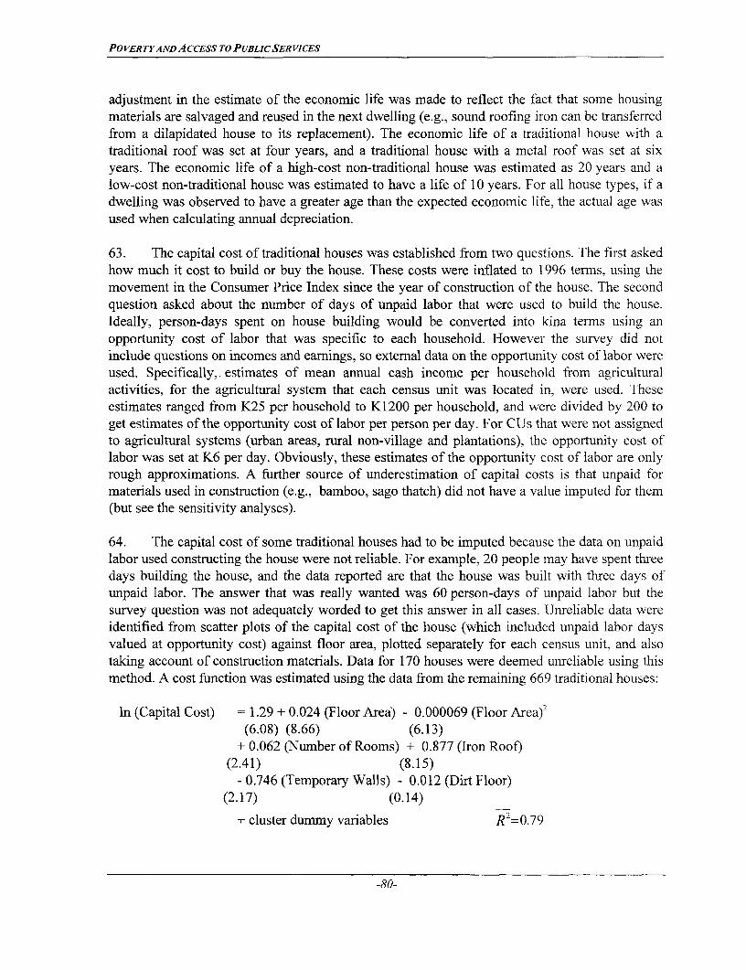
POVERTYAND ACCESS TO PUBLICSERVICES
adjustment in the estimate of the economic life was made to reflect the fact that some housingmaterials are salvaged and reused in the next dwelling (e.g., sound roofing iron can be transferredfrom a dilapidated house to its replacement). The economic life of a traditional house with atraditional roof was set at four years, and a traditional house with a metal roof was set at sixyears. The economic life of a high-cost non-traditional house was estimated as 20 years and alow-cost non-traditional house was estimated to have a life of 10 years. For all house types, if adwelling was observed to have a greater age than the expected economic life, the actual age wasused when calculating annual depreciation.
63. The capital cost of traditional houses was established from two questions. The first askedhow much it cost to build or buy the house. These costs were inflated to 1996 terms, using themovement in the Consumer Price Index since the year of construction of the house. The secondquestion asked about the number of days of unpaid labor that were used to build the house.Ideally, person-days spent on house building would be converted into kina terms using anopportunity cost of labor that was specific to each household. However the survey did notinclude questions on incomes and earnings, so external data on the opportunity cost of labor wereused. Specifically,. estimates of mean annual cash income per household from agriculturalactivities, for the agricultural system that each census unit was located in, were used. Theseestimates ranged from K25 per household to K1200 per household, and were divided by 200 toget estimates of the opportunity cost of labor per person per day. For CUs that were not assignedto agricultural systems (urban areas, rural non-village and plantations), the opportunity cost oflabor was set at K6 per day. Obviously, these estimates of the opportunity cost of labor are onlyrough approximations. A further source of underestimation of capital costs is that unpaid formaterials used in construction (e.g., bamboo, sago thatch) did not have a value imputed for them(but see the sensitivity analyses).
64. The capital cost of some traditional houses had to be imputed because the data on unpaidlabor used constructing the house were not reliable. For example, 20 people may have spent threedays building the house, and the data reported are that the house was built with three days ofunpaid labor. The answer that was really wanted was 60 person-days of unpaid labor but thesurvey question was not adequately worded to get this answer in all cases. Unreliable data wereidentified from scatter plots of the capital cost of the house (which included unpaid labor daysvalued at opportunity cost) against floor area, plotted separately for each census unit, and alsotaking account of construction materials. Data for 170 houses were deemed unreliable using thismethod. A cost function was estimated using the data from the remaining 669 traditional houses:
ln (Capital Cost) = 1.29 + 0.024 (Floor Area) - 0.000069 (Floor Area)2
(6.08) (8.66) (6.13)+ 0.062 (Number of Rooms) + 0.877 (Iron Roof)
(2.41) (8.15)- 0.746 (Temporary Walls) - 0.012 (Dirt Floor)
(2.17) (0.14)
+ cluster dummy variables R2=0.79
-80-
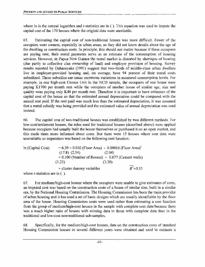
POVERTYAND AccEss TO PUBLICSERVICES
where In is the natural logarithm and t-statistics are in (). This equation was used to impute thecapital cost of the 170 houses where the original data were unreliable.
65. Estimating the capital cost of non-traditional houses was more difficult. Fewer of theoccupiers were owners, especially in urban areas, so they did not know details about the age ofthe dwelling or construction costs. In principle, this should not matter because if these occupiersare paying rent, their rental payments serve as an estimate of the consumption of housingservices. However, in Papua New Guinea the rental market is distorted by shortages of housing(due partly to collective clan ownership of land) and employer provision of housing. Surveyresults reported by Dahanayake (1991) suggest that two-thirds of middle-class urban dwellerslive in employer-provided housing and, on average, have 94 percent of their rental costssubsidized. These subsidies can cause enormous variations in measured consumption levels. Forexample, in one high-cost Census Unit in the NCD sample, the occupiers of one house werepaying K1700 per month rent while the occupiers of another house of similar age, size andquality were paying only K40 per month rent. Therefore it is important to have estimates of thecapital cost of the house so that the estimated annual depreciation could be compared with theannual rent paid. If the rent paid was much less than the estimated depreciation, it was assumedthat a rental subsidy was being provided and the estimated value of annual depreciation was usedinstead.
66. The capital cost of non-traditional houses was established by two different methods. Forlow-cost/settlement houses, the rules used for traditional houses (described above) were appliedbecause occupiers had usually built the house themselves or purchased it on an open market, andthis made them more informed about costs. But there were 15 houses where cost data wereunavailable so imputation was based on the following cost function:
In (Capital Cost) = 6.39 + 0.030 (Floor Area) - 0.00016 (Floor Area)2
(17.8) (2.54) (2.04)+ 0.100 (Number of Rooms) + 0.677 (Cement walls)
(1.23) (3.20)
+ cluster dummy variables R2=0.33where t-statistics are in ( ).
67. For medium/high-cost houses where the occupiers were unable to give estimates of costs,an imputed cost was based on the construction costs of a house of similar size, built in a similarera, by the National Housing Commission. The Housing Commission has been the main providerof urban housing and it has used a set of basic designs which are usually identifiable by the floorarea of the house. Housing Commission costs were used rather than estimating a cost functionfrom the group of medium/high-cost houses in the sample with complete cost data because therewas a much higher ratio of houses with missing data to those with complete data than in thetraditional and low-cost non-traditional sub-samples.
68. Specifically, for the medium/high-cost houses, data on the construction costs of standardHousing Commission houses in several different years were obtained and used to estimate a
-81-
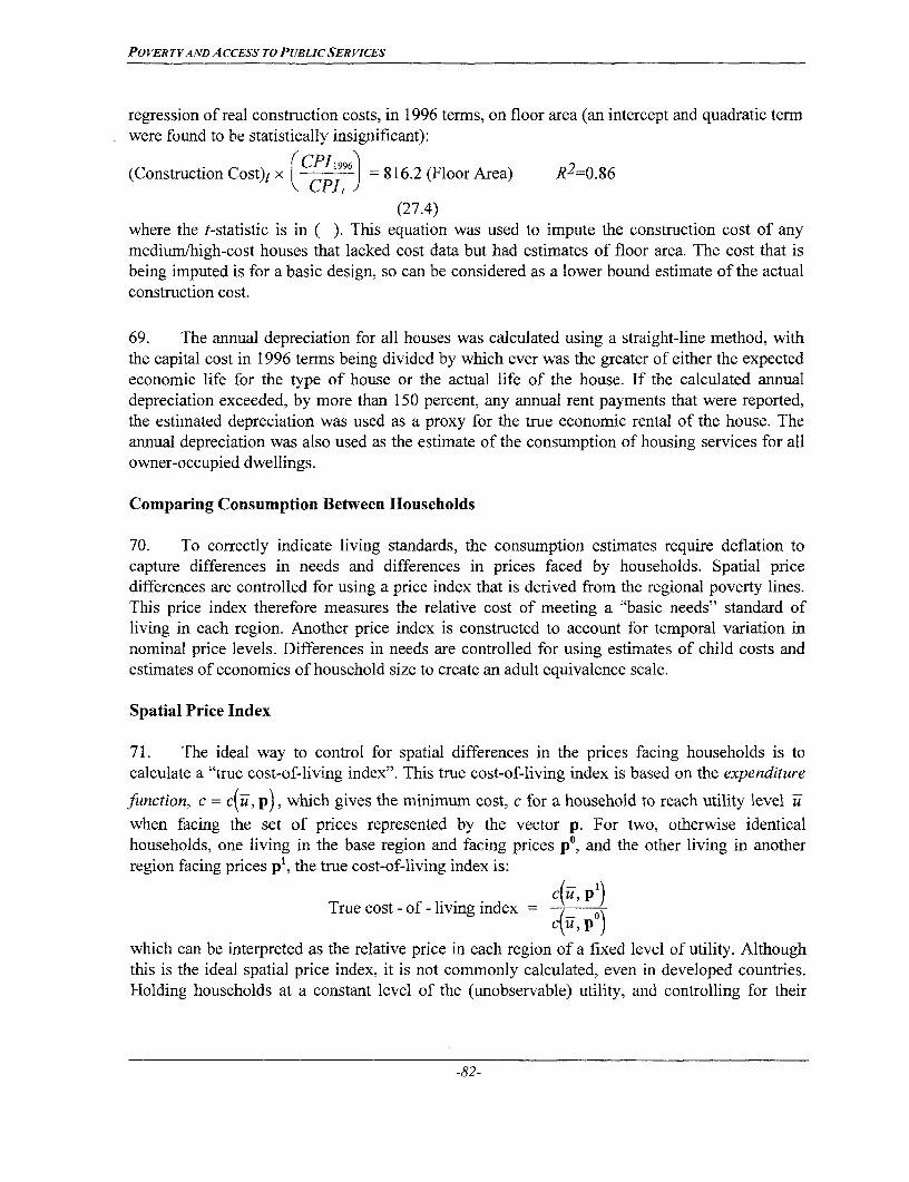
POVERTYAND A CCESS To PUBLIC SERvICES
regression of real construction costs, in 1996 terms, on floor area (an intercept and quadratic termwere found to be statistically insignificant):
(CPI1996\(Construction Cost)t x ( _) = 816.2 (Floor Area) R2 =0.86
(27.4)where the t-statistic is in ( ). This equation was used to impute the construction cost of anymedium/high-cost houses that lacked cost data but had estimates of floor area. The cost that isbeing imputed is for a basic design, so can be considered as a lower bound estimate of the actualconstruction cost.
69. The annual depreciation for all houses was calculated using a straight-line method, withthe capital cost in 1996 terms being divided by which ever was the greater of either the expectedeconomic life for the type of house or the actual life of the house. If the calculated annualdepreciation exceeded, by more than 150 percent, any annual rent payments that were reported,the estimated depreciation was used as a proxy for the true economic rental of the house. Theannual depreciation was also used as the estimate of the consumption of housing services for allowner-occupied dwellings.
Comparing Consumption Between Households
70. To correctly indicate living standards, the consumption estimates require deflation tocapture differences in needs and differences in prices faced by households. Spatial pricedifferences are controlled for using a price index that is derived from the regional poverty lines.This price index therefore measures the relative cost of meeting a "basic needs" standard ofliving in each region. Another price index is constructed to account for temporal variation innominal price levels. Differences in needs are controlled for using estimates of child costs andestimates of economies of household size to create an adult equivalence scale.
Spatial Price Index
71. The ideal way to control for spatial differences in the prices facing households is tocalculate a "true cost-of-living index". This true cost-of-living index is based on the expenditure
function, c = c(u, p), which gives the minimum cost, c for a household to reach utility level u
when facing the set of prices represented by the vector p. For two, otherwise identicalhouseholds, one living in the base region and facing prices p°, and the other living in anotherregion facing prices pl, the true cost-of-living index is:
True cost - of - living index = C(W, p')c(ii, po)
which can be interpreted as the relative price in each region of a fixed level of utility. Althoughthis is the ideal spatial price index, it is not commonly calculated, even in developed countries.Holding households at a constant level of the (unobservable) utility, and controlling for their
-82-
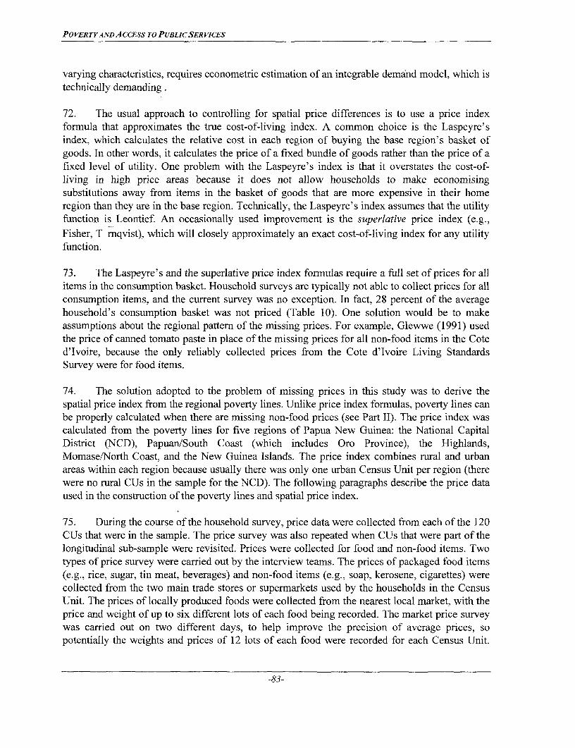
POVERTYAND A CCESS To PUBLICSER VICES
varying characteristics, requires econometric estimation of an integrable demand model, which istechnically demanding.
72. The usual approach to controlling for spatial price differences is to use a price indexformula that approximates the true cost-of-living index. A common choice is the Laspeyre'sindex, which calculates the relative cost in each region of buying the base region's basket ofgoods. In other words, it calculates the price of a fixed bundle of goods rather than the price of afixed level of utility. One problem with the Laspeyre's index is that it overstates the cost-of-living in high price areas because it does not allow households to make economisingsubstitutions away from items in the basket of goods that are more expensive in their homeregion than they are in the base region. Technically, the Laspeyre's index assumes that the utilityfunction is Leontief. An occasionally used improvement is the superlative price index (e.g.,Fisher, T mqvist), which will closely approximately an exact cost-of-living index for any utilityfunction.
73. The Laspeyre's and the superlative price index formulas require a full set of prices for allitems in the consumption basket. Household surveys are typically not able to collect prices for allconsumption items, and the current survey was no exception. In fact, 28 percent of the averagehousehold's consumption basket was not priced (Table 10). One solution would be to makeassumptions about the regional pattern of the missing prices. For example, Glewwe (1991) usedthe price of canned tomato paste in place of the missing prices for all non-food items in the Coted'Ivoire, because the only reliably collected prices from the Cote d'Ivoire Living StandardsSurvey were for food items.
74. The solution adopted to the problem of missing prices in this study was to derive thespatial price index from the regional poverty lines. Unlike price index formulas, poverty lines canbe properly calculated when there are missing non-food prices (see Part II). The price index wascalculated from the poverty lines for five regions of Papua New Guinea: the National CapitalDistrict (NCD), Papuan/South Coast (which includes Oro Province), the Highlands,Momase/North Coast, and the New Guinea Islands. The price index combines rural and urbanareas within each region because usually there was only one urban Census Unit per region (therewere no rural CUs in the sample for the NCD). The following paragraphs describe the price dataused in the construction of the poverty lines and spatial price index.
75. During the course of the household survey, price data were collected from each of the 120CUs that were in the sample. The price survey was also repeated when CUs that were part of thelongitudinal sub-sample were revisited. Prices were collected for food and non-food items. Twotypes of price survey were carried out by the interview teams. The prices of packaged food items(e.g., rice, sugar, tin meat, beverages) and non-food items (e.g., soap, kerosene, cigarettes) werecollected from the two main trade stores or supermarkets used by the households in the CensusUnit. The prices of locally produced foods were collected from the nearest local market, with theprice and weight of up to six different lots of each food being recorded. The market price surveywas carried out on two different days, to help improve the precision of average prices, sopotentially the weights and prices of 12 lots of each food were recorded for each Census Unit.
-83-

POVERTYAND ACCESS TO PUBLIC SERVICES
However in some areas markets were held only infrequently so the price survey could be carriedout only once. In a few cases, interviewers made special return visits to an area to coincide withmarket day.
Table 10: Average Budget Shares of Consumption Items That Were Not Priced
Firewood 6.182 Jewellery, watches, clocks, umbrellas, bags 0.173
P.M.V. fares 3.129 Medicines (modem and traditional) 0.162
Wedding expenses and brideprice 2.443 Life, health and personal effects insurance 0.128
Meals consumed away from home 2.094 Entertainment equipment (toys, books,..) 0.127
Depreciation of non-housing durables 1.994 School stationary, text books & uniforms 0.126
Adult's clothing (new and used) 1.468 Charges for sewerage, garbage and water 0.112
School fees (tuition and boarding) 1.428 Other home maintenance products 0.092
Airfares, ship fares, car hire 1.162 Domestic services 0.091
Compensation payments 1.061 Vehicle registration and insurance charges 0.090
Gambling (except lottery tickets) 1.054 Toilet paper 0.084
Children's clothing 0.953 Diesel 0.078
Burial and death feast expenses 0.621 Lottery tickets 0.073
Linen 0.534 Entrance fees for films and videos 0.066
Kitchen utensils 0.466 Telephone charges 0.058
Medical fees 0.348 Other household equipment and services 0.054
Footwear 0.343 Fumishings 0.042
Household and garden tools 0.285 House repairs and maintenance 0.038
Vehicle repairs and maintenance 0.222 Entrance fees to sports matches 0.036
Electricity and gas charges 0.201 Stamps and postage fees 0.029
Newspapers and magazines 0.183 Holiday accommodation and tours 0.022
Other personal care products 0.173 Land rent and land taxes for the section 0.013
Kitchen electrical equipment 0.010
Total budget share 28.191
76. The average price of each item was calculated for each Census Unit. For items from thetrade store survey, this usually meant taking an average of two prices, but if the item was onlyavailable in one store the single price was used. Sometimes the items available were not of thedesired specification (e.g., the specification for tinned meat was a 340g can of "Ox and Palm"brand, but sometimes the price collected may have been for a 200g can, or for a 340g can of adifferent brand). When the price for the non-specification good was the only one available in aparticular Census Unit it was used to predict the missing price of the good of desiredspecification, if price relativities between that specification and the desired specification wereable to be estimated from the rest of the sample. Otherwise, the missing price was predicted froma cross-sectional regression of the price of the desired item on the prices of all other trade storegoods, for the sample of CUs where the price was not missing. The logic of this regression is thatthe spatial pattern of prices for trade store goods reflects transport costs.
-84-

POVERTYANDACCESS TOPUBLICSERVICES
77. An exception to these procedures was made for the CUs in the NCD sample, where asimple average was taken of the prices for each item collected in all 40 CUs. The reason for thisexception was that people who live in one part of the capital city can easily buy in other parts ofthe city. Therefore the spatial distribution of prices inside Port Moresby is less relevant than isthe spatial distribution of prices within the other, larger, regions.
78. If a locally produced food was not able to be priced in a particular Census Unit during thesurvey period, the price was treated as missing data and was not predicted. There are two reasonsfor treating the prices of locally grown foods in a different manner to the treatment for packagedfood items. First, the reasons for not observing a price are more complex: the Census Unit maylie outside the environmental range of production for the food, or the crop may be available inonly certain seasons of the year, or in more remote areas the food could be so widely grown thatno market exists because demand is meet by own-production. Second, there is no single factorlike transport costs that could be used for predicting the price.
79. The collection of prices spanned 12 months so there will be temporal as well as spatialvariation. The temporal variation should not affect the average prices calculated for the fourregions outside of the NCD because surveying progressed at approximately the same pace inthose four regions. However, the NCD survey did not start until April, three months after the firstprices were collected in the other regions. The quarterly Consumer Price Index, calculated by theNSO, was used to correct for the different distribution across time of the samples. Specifically, aweighted average of the CPI was taken for the non-NCD sample, where the weights were thenumber of CUs surveyed in each quarter. A similar average was taken for the NCD sample andthe ratio of the two was estimated as 1.0051. Therefore, all prices collected in the NCD surveywere reduced by a factor of 1/1.0051, so as to be directly comparable, timewise, whencomparisons were being made with the prices collected in the other regions.
80. Some items were priced at regional level because market prices for these items are notwidely available in all Census Units. This included formally marketed items that are sold mainlyin urban areas (such as bread, lamb and mutton) and informally marketed items produced in onlya few areas but sold more widely throughout urban markets (e.g., potatoes).
81. One important item of consumption whose price is not directly observable, and wastherefore not collected during the price survey, is the consumption of housing services. Instead,the implicit price of housing services in each region was computed by regressing the logarithm ofannual rents (actual and imputed) on a vector of housing characteristics. The vector ofcharacteristics included: the floor area of the house, the number of rooms, the material of thewalls (four dummy variables), the material of the floor (four dummy variables), and the materialof the roof (two dummy variables). The equation also included dummy variables for the fourregions outside of the NCD. The sample excluded dwellings whose capital cost was imputed(equations in paragraph 65 and 67) and dwellings with subsidized rents and insufficientinformation to estimate annual depreciation. In total, 918 observations were available (76 percentof the total). The results were:
-85-
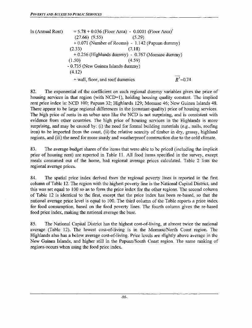
POVERTYAND ACCESS TO PUBLICSERVICES
In (Annual Rent) = 5.78 + 0.036 (Floor Area) - 0.0001 (Floor Area)2
(27.66) (9.55) (5.29)+ 0.071 (Number of Rooms) - 1.142 (Papuan dummy)
(2.33) (7.18)+ 0.256 (Highlands dummy) - 0.767 (Momase dummy)
(1.50) (4.59)- 0.735 (New Guinea Islands dummy)(4.12)
+ wall, floor, and roof dummies R2=0.74
82. The exponential of the coefficient on each regional dummy variables gives the price ofhousing services in that region (with NCD=1), holding housing quality constant. The impliedrent price index is: NCD 100; Papuan 32; Highlands 129; Momase 46; New Guinea Islands 48.There appear to be large regional differences in the (constant-quality) price of housing services.The high price of rents in an urban area like the NCD is not surprising, and is consistent withevidence from other countries. The high price of housing services in the Highlands is moresurprising, and may be caused by: (i) the need for formal building materials (e.g., nails, roofingiron) to be imported from the coast, (ii) the relative scarcity of timber in dry, grassy, highlandregions, and (iii) the need for more sturdy and weatherproof construction due to the cold climate.
83. The average budget shares of the items that were able to be priced (including the implicitprice of housing rent) are reported in Table 11. All food items specified in the survey, exceptmeals consumed out of the home, had regional average prices calculated. Table 2 lists theregional average prices.
84. The spatial price index derived from the regional poverty lines is reported in the firstcolumn of Table 12. The region with the highest poverty line is the National Capital District, andthis was set equal to 100 so as to form the price index for the other regions. The second columnof Table 12 is identical to the first, except that the price index has been re-based, so that thenational average price level is equal to 100. The third column of the Table reports a price indexfor food consumption, based on the food poverty lines. The fourth column gives the re-basedfood price index, making the national average the base.
85. The National Capital District has the highest cost-of-living, at almost twice the nationalaverage (Table 12). The lowest cost-of-living is in the Momase/North Coast region. TheHighlands also has a below average cost-of-living. Price levels are slightly above average in theNew Guinea Islands, and higher still in the Papuan/South Coast region. The same ranking ofregions occurs when using the food price index.
-86-
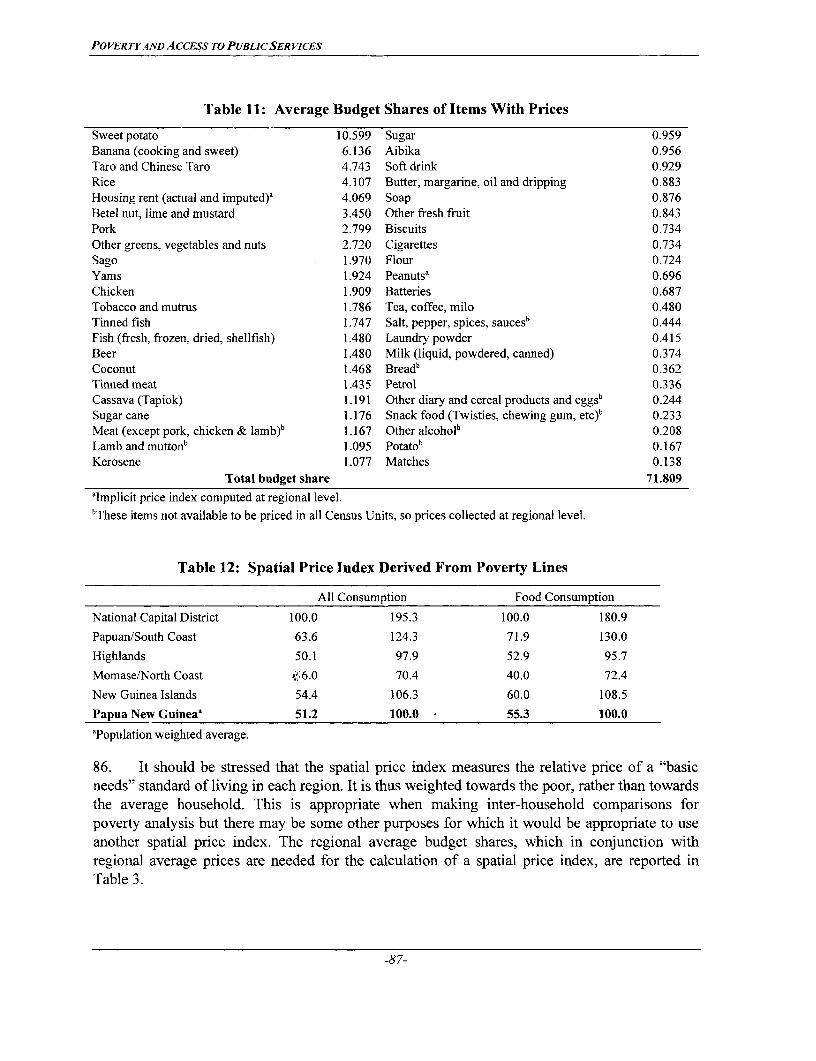
POVERTYAND ACCESS TO PUBLICSERviCES
Table 11: Average Budget Shares of Items With Prices
Sweet potato 10.599 Sugar 0.959Banana (cooking and sweet) 6.136 Aibika 0.956Taro and Chinese Taro 4.743 Soft drink 0.929Rice 4.107 Butter, margarine, oil and dripping 0.883Housing rent (actual and imputed)a 4.069 Soap 0.876Betel nut, lime and mustard 3.450 Other fresh fruit 0.843Pork 2.799 Biscuits 0.734Other greens, vegetables and nuts 2.720 Cigarettes 0.734Sago 1.970 Flour 0.724Yams 1.924 Peanutsa 0.696Chicken 1.909 Batteries 0.687Tobacco and mutrus 1.786 Tea, coffee, milo 0.480Tinned fish 1.747 Salt, pepper, spices, saucesb 0.444Fish (fresh, frozen, dried, shellfish) 1.480 Laundry powder 0.415Beer 1.480 Milk (liquid, powdered, canned) 0.374Coconut 1.468 Breadb 0.362Tinned meat 1.435 Petrol 0.336Cassava (Tapiok) 1.191 Other diary and cereal products and eggsb 0.244Sugar cane 1.176 Snack food (Twisties, chewing gum, etc)b 0.233Meat (except pork, chicken & lamb)b 1.167 Other alcoholb 0.208Lamb and muttonb 1.095 Potatob 0.167Kerosene 1.077 Matches 0.138
Total budget share 71.809almplicit price index computed at regional level.bThese items not available to be priced in all Census Units, so prices collected at regional level.
Table 12: Spatial Price Index Derived From Poverty Lines
All Consumption Food Consumption
National Capital District 100.0 195.3 100.0 180.9
Papuan/South Coast 63.6 124.3 71.9 130.0
Highlands 50.1 97.9 52.9 95.7
MomaselNorth Coast 4 6. 0 70.4 40.0 72.4
New Guinea Islands 54.4 106.3 60.0 108.5
Papua New Guineaa 51.2 100.0 * 55.3 100.0
aPopulation weighted average.
86. It should be stressed that the spatial price index measures the relative price of a "basicneeds" standard of living in each region. It is thus weighted towards the poor, rather than towardsthe average household. This is appropriate when making inter-household comparisons forpoverty analysis but there may be some other purposes for which it would be appropriate to useanother spatial price index. The regional average budget shares, which in conjunction withregional average prices are needed for the calculation of a spatial price index, are reported inTable 3.
-87-

POVERTYAND ACCESS TO PUBLIC SER VICES
Temporal Price Index
87. Ideally temporal price variation should be controlled for at the same time that spatialprice variation is controlled for. However, the composition of the sample changed from month tomonth, tending in some months to be more remote than in others. Thus, the comparison ofaverage monthly prices may pick up more than just temporal variation. The only temporalcomparisons of prices that avoid this problem are for the 20 clusters revisited as part of thelongitudinal sub-sample. However, these revisits did not start until after June, so a March quarterto June quarter price comparison is unavailable.
88. Instead of using the prices collected by the survey, variation in nominal price levels overthe 12 month period of the field work was controlled for by using the Consumer Price Index as adeflator (Table 3). The deflator was applied uniformly to each region. It should be stressed thatthe CPI is actually calculated just for urban areas so it may not be an ideal guide to intra-yearchanges in the cost of living for the whole of PNG in 1996.
Table 13: Temporal Price Deflator
March June September December AnnualIndex 344.4 345.9 351.4 350.8 348.1Deflator 98.9 99.4 100.9 100.8 100.0
Adjusting For Differences in Household Composition
89. A household with small children may not need as much consumption expenditure to reachthe same standard of living as a similarly sized household where all of the members are adults.Earlier research in PNG used consumption per adult-equivalent, where children aged less than15 years count as 0.5 adult-equivalents but this scale was not based on actual measurements ofchild costs. Recently, Gibson (1996) estimated child costs using data from the Urban HouseholdSurvey, and found that a scale of 0.5 was appropriate for young children (0-6 years) but olderchildren had the same cost as adults.
90. Adjusting for differences in needs only matters if the share of children in householdnumbers varies widely between households (or between population sub-groups). If children'sdemographic share is roughly constant, the correction factor to convert household numbers intoadult equivalents would also be roughly constant and would not lead to much re-ranking ofhouseholds, compared with a rank formed over per capita expenditure. In fact, there is a lot ofvariation in the share of children in household numbers. The share of the six-years-and-under agegroup is 20 percent on average, but ranges from zero to 80 percent. There is also variation betweenthe averages for each region, ranging from a 17 percent share in the NCD to a 22 percent share inthe South Coast and Momase regions. Hence, treating young children like adults, and giving them aweight of 1.0 when forming per capita consumption might lower the estimated standard of livingfor households in the Momase and South Coast regions relative to NCD households, if in factyoung children have fewer needs than adults.
-88-

PO VERTYAND A CC-ESS TO PUBLIC SER VICES
91. here are two main methods of measuring child costs: the Engel method and the Rothbarthmethod. The Engel method is based on the assumption that a household's standard of living isindicated by its budget share for food. The cost of an additional child can be measured bycalculating the amount of compensation that would have to be paid to the parents to maintain thesame food share as before the child was born. The Rothbarth method assumes that adults' standardof living is indicated by the value of expenditure on "adult goods" (goods not consumed bychildren). Expenditures on adult goods should fall when children are added to the householdbecause the child brings additional consumption needs without any offsetting increase in income.Therefore, the cost of an additional child can be measured by calculating the amount ofcompensation that would have to be paid to parents to restore expenditure on adult goods to theformer level. Deaton and Muellbauer (1986) show that the Engel method overestimates the cost ofchildren, while the Rothbarth method underestimates them, so the two methods are used here to setbounds on the adult equivalence scale for children.
92. he food Engel curve used by Deaton and Muellbauer (1986) is of the form:
Wf= Cc-/6In(-JY~j nj +8.-v + ( n)+ Jj=
where Wf is the food budget share, x is total expenditure, n is the total number of people in thehousehold, nj is the number of persons in category j (=1, . . , J), v is a vector of other control
variables, [I is a random error, and D, [, Cl and 6 are parameters. The food Engel curve wasestimated using three demographic groups: na, ncl, and nc2, which are the number of adults, thenumber of older children (age 7 to 14), and the number of young children (O to 6 years). Totalhousehold expenditure, x was deflated by the value of the food poverty line (in index form), zf.Dummy variables for each region were included as controls for price and non-price variation thataffect the food budget share. Results are reported in column (i) of Table 14.
Table 14: Estimates of Food Engel Curves
Explanatory variable (i) (ii)
In real per capita expenditure [(xlzj/ln] -0.0511(2.93)
In real household expenditure [xIzA ... -0.0523(2.94)
In household size ... 0.0109(0.31)
Number of adults -0.0066 -0.0000(1.97) (0.00)
Number of older children -0.0004 0.0072(0.07) (0.86)
Number of young children -0.0077 -0.0001(1.20) (0.01)
Intercept 0.813 0.841
R2 0.130 0.132Note: Absolute t-values in ()corrected for clustering, sampling weights and stratification.Regional dummy variables also included in each equation. N= 1144.
-89-

POVERTYAND A CCESS To PUBLICSERViCES
93. For the specification in column (i) the food budget share for the reference household withtwo adults and no children is given by:
wf = a + flnxx -,Bln2 + y1 .2
where y, is the coefficient on the number of adults, and the regional dummy variables and the foodprice deflator have been suppressed for convenience. For another household in the same region, buthaving two adults and an older child, the food budget share is given by:
wj = a + ,6lnxl -,/ln3 + y, 2 +72 1,
where y2 is the coefficient on the number of older children. Under the Engel assumption, the twohouseholds are equally as well off when their food shares are equal. Therefore, setting these twoequations equal to one and other and solving for x gives the equivalence scale:
In x = 2 - ln.x 0 8 3
94. Household total expenditure has to rise by 49 percent when an older child is added, so anolder child appears to cost just as much as an adult. Replacing y2 with y3 (the coefficient on thenumber of younger children) in the formula indicates that household total expenditure has to rise by29 percent when a younger child is added, so the adult-equivalence of that child is 0.58. In general,for this Engel curve, the equivalence scale for household h to reach the same welfare level as thereference household 0 is:
Eh (n-h)exp J-p)(nh - nO)].
95. The specification used for the results reported in column (i) of Table 14 imposes ahomogeneity assumption, by using per capita expenditure. A more flexible specification, whichwill also be useful for estimating household size economies, is to allow the logarithm of realhousehold expenditure and the logarithm of household size to enter the equation as separatevariables. For this specification, the equivalence scale for adding an older child to the referencehousehold with two adults is given by:
x 7 2 1 3x 0 = - 2
where ri is the coefficient on the logarithm of household size. Results for this model are reported incolumn (ii) of Table 14. Household total expenditure has to rise by 25 percent when an older childis added to the reference household, so the adult-equivalence of that child is 0.50. For a youngerchild the adult equivalence is 0.18.
96. The adult-equivalence scale derived from the results in column (ii) shows surprisingly lowcosts of children in comparison with earlier estimates for PNG and other countries. This isespecially because, in theory, the Engel method overestimates the cost of children. Which resultsshould be used? The homogeneity assumption to derive the column (i) specification from thecolumn (ii) specification (r/,=-1) is not rejected, with X2(1) =1.4 (p<0.24). Thus, statistical testing
-90-
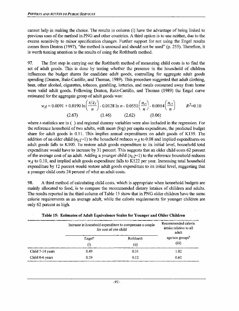
POVERTYAND ACCESS To PuBLic SER VICES
cannot help in making the choice. The results in column (i) have the advantage of being linked toprevious uses of the method in PNG and other countries. A third option is to use neither, due to theexcess sensitivity to minor specification changes. Further support for not using the Engel resultscomes from Deaton (1997), "the method is unsound and should not be used" (p. 255). Therefore, itis worth turning attention to the results of using the Rothbarth method.
97. The first step in carrying out the Rothbarth method of measuring child costs is to find theset of adult goods. This is done by testing whether the presence in the household of childreninfluences the budget shares for candidate adult goods, controlling for aggregate adult goodsspending (Deaton, Ruiz-Castillo, and Thomas, 1989). This procedure suggested that adult clothing,beer, other alcohol, cigarettes, tobacco, gambling, lotteries, and meals consumed away from homewere valid adult goods. Following Deaton, Ruiz-Castillo, and Thomas (1989) the Engel curveestimated for the aggregate group of adult goods was:
WA =O0.0091 +o0.0190 In('j - 0.0128 In n - 0.0551 (-)- 0.0014 (-) R2=0.I0
(2.67) (1.46) (2.62) (0.06)
where t-statistics are in ( ) and regional dummy variables were also included in the regression. Forthe reference household of two adults, with mean (log) per capita expenditure, the predicted budgetshare for adult goods is 0.11. This implies annual expenditures on adult goods of K139. Theaddition of an older child (ncl=l) to the household reduces wA to 0.08 and implied expenditures onadult goods falls to K100. To restore adult goods expenditure to its initial level, household totalexpenditure would have to increase by 31 percent. This suggests that an older child costs 62 percentof the average cost of an adult. Adding a younger child (nc2=1 ) to the reference household reducesWA to 0.10, and implied adult goods expenditure falls to K1 22 per year. Increasing total householdexpenditure by 12 percent would restore adult goods expenditure to its initial level, suggesting thata younger child costs 24 percent of what an adult costs.
98. A third method of calculating child costs, which is appropriate when household budgets aremainly allocated to food, is to compare the recommended dietary intakes of children and adults.The results reported in the third column of Table 15 show that in PNG older children have the samecalorie requirements as an average adult, while the calorie requirements for younger children areonly 62 percent as high.
Table 15: Estimates of Adult Equivalence Scales for Younger and Older Children
Increase in household expenditure to compensate a couple Recommended caloriefor cost of one child intake relative to all
adult
Engela Rothbarth age/sex groupsb
(i (ii) (iii)
Child7-14years 0.49 0.31 1.02
Child 0-6 years 0.29 0.12 0.62
-91-
POVERTYANDACCESS TO PUBLIC SERVICES
aUsing the results in column (iii) of Table 14.bCalculated from requirements in Nutritionfor Papua New Guinea, Department of Health (1975)
99. The two most reliable methods of calculating child costs (Rothbarth and calorierequirements) suggest that the adult-equivalence of a 7-14 year old child is between 0.62 and 1.02 .The adult equivalence of younger children lies between 0.24 and 0.62 according to these same twomethods. The most plausible estimates from the Engel method are for the specification used byDeaton and Muellbauer (1986). Those Engel estimates are similar to the results using calorierequirements, with older children costing 98 percent of an adult, and younger children costing 58percent of an adult. In view of these results, the equivalence scale used here is that children age sixyears and below count as 0.5 adult-equivalents, and everyone else counts as 1.0.
Adjusting for Differences in Household Size
100. Economies of size in household consumption allow the cost per person of reaching a certainstandard of living to fall as household size rises. For example, a household with ten people may notneed to spend ten times as much as a single-person household to enjoy the same standard of living.Economies of size can affect two types of poverty comparisons. The first is between demographicgroups, such as "small" households and "large" ones. When no allowance is made for economies ofsize, large households typically appear to be poorer (Lanjouw and Ravallion, 1995). Thiscorrelation may lead policy makers to use "demographic targeting" to alleviate poverty by makingprograms specially available to large households. If in fact the lower per capita expenditure by largehouseholds just reflects economies of size, such demographically targeted policies are a wastefulway of alleviating poverty. Secondly, unaccounted for economies of size can distort regionalpoverty profiles because estimates of poverty will be too high for regions with larger householdsand too low for regions with smaller households. This could affect poverty comparisons betweenthe NCD and other regions, because the average household size in the NCD (6.9 dwellers perhousehold) is 25 percent higher than in other regions.
101. A modified Engel method of measuring size economies has recently been introduced byLanjouw and Ravallion (1995). Instead of deflating total expenditure by person numbers, n, theydeflate by equivalent person numbers, n9 (0<•01), where 0 is the size elasticity of the cost of living.
Noting that ,l1n(x/n9) can also be expressed as f)lnx-0,8lnn, the Engel curve can be estimatedwith lnx and lnn as separate variables, and the ratio of the coefficient on lnn to the coefficient onlnx gives an estimate of 0. This estimate of the size elasticity of the cost of living applies only tohouseholds of the same composition. When demographic composition is controlled for using thenumbers of persons, as in Table 14, the size elasticity is calculated as:
O= -17 + J n
where rl is the coefficient on Inn, ,B is the coefficient on lnx, yj is the coefficient on the numberof people in the household from the jth demographic group, niln is the share for the jth
-92-

POVERTYAND ACCESS TO PUBLICSERVICES
demographic group, and n is household size. Using the coefficient estimates in column (ii) ofTable 14, and population averages for nj and n, the calculated size elasticity is 0.34 with a standarderror of 0.25.
102. These results have important implications for the measurement of living standards. Thehypothesis that per capita expenditure is the correct variable for comparing households of differentsizes (i.e., 9=1) is rejected, with X2(l)=6.14 (p<0.02). The hypothesis that no adjustment for size isneeded when comparing different households (i.e., 9=0) is not rejected, with X2(l,l .90 (p<0. 17). Inother words, the data do not reject the hypothesis that each person in the household, beyond the firstresident, costs nothing. Under this hypothesis, all items in the household's budget have non-rivalconsumption, which is not a plausible description of items like food. Thus, something appearswrong with this method of measuring household size economies.
103. One improvement is to drop the three demographic composition terms (na, ncl, and nc2)from the model because they are not statistically significant (p<0.67). With this change, the valueobtained for a is 0.41, with a standard error of 0.22. The assumption of homogeneity (*=1) is stillrejected, with X2(,)=6.88 (p<0.0l). The other hypothesis, that no adjustment for number of residentsis needed when comparing different households (90), is now rejected only at relaxed levels ofstatistical significance, with X2(,)-3 .36 (p<0.07).
104. The Engel method of measuring household size economies has been criticised by Deatonand Paxson (1996). The criticism is that as household size increases the sharing of public goodswithin the household should free up resources that will increase the demand for a (poorlysubstitutable) private good like food. Thus, there should be a positive relationship betweenhousehold size and food demand, holding outlay per person constant. Instead, the results reportedhere, the results of Lanjouw and Ravallion for Pakistan, and results in a number of other countries,show the budget share for food (and therefore food consumption, unless pecuniary effects are verystrong) falling with household size, at constant per capita outlay. The experiment comparing theperformance of the recall survey instrument with the diary survey instrument in the NCD may be ofrelevance. For households surveyed using the recall instrument, the food share fell with increases inhousehold size, holding outlay per person constant. However, for the matched households who usedthe diary survey, there is no relationship between the food share and household size, with outlay perperson held constant. One interpretation of this is that there are measurement errors in foodexpenditures that are correlated with household size (Gibson, 1997). If this is the case, the estimateof 0.41 for the size elasticity of the cost of living may overstate the true extent of household sizeeconomies.
105. It may be appropriate to use another welfare indicator for estimating size economies, inview of the problems in using the budget share for food. The Rothbarth assumption, that adultgoods expenditure indicates (adult) welfare levels may be useful. But in contrast to the case ofestimating child costs, total spending on adult goods is no longer an appropriate welfare indicatorbecause some of the additions to the household will be adults, whose presence would reduce per
-93-

POVERTY AND ACCESS To PUBLIC SERVICES
adult consumption of adult goods. Instead, adult goods expenditure per adult is used as the welfareindicator. The equation estimated for the aggregate group of adult goods is
PA qA = -193.3 +252.0 lnx -307.7 Inn -201.9 ( -74.1 (nl) R2=0.24nA n n
(4.90) (5.34) (1.90) (0.97)
where PA qA is expenditure on adult goods, nA is the number of adults, t-statistics are in (), andthe equation also includes regional dummy variables. The size elasticity is given by the ratio of thecoefficient on ln n to the coefficient on ln x, which is 1.22 (standard error of 0.1 1). This implies thatto maintain a constant value of adult goods consumption per adult, household total expenditure hasto increase by at least the same percentage as the increase in household size. If the welfare indicatorused was the budget share for adult goods, the hypothesis that OA1 is also not rejected (p<0.30).Thus, in contrast to the results using the food budget share, methods using adult goods as thewelfare indicator do not find economies of household size.
106 What can be made of these diverse estimates of the extent of household size economies?Although it is possible that x/n 0 4' is the correct indicator of living standards, the Engel method doesnot seem sufficiently uncontroversial and its results may be affected by measurement error.Therefore, the main analyses in this report follow usual procedure and do not adjust for sizeeconomies.
107. To explore the robustness of the results in Table 1.6 of the main report, poverty measuresfor varying household size groups were recalculated using two economy of size correction factors:0.7 which is about equal to the poor's food expenditure share and 0.41 which is the correctionfactor that was estimated from this data set (Tables 16 and 17). The analysis shows that povertymeasures for larger households drop significantly, while those for smaller households increasewhen household economy correction factors are employed. However, given the controversysurrounding the setting of the correction factor, it is preferable to follow standard practice and notadjust household consumption for size economies for the poverty profile in this report.Nevertheless, the marked difference in the poverty measures for various household size groupswhen correction factors are employed, suggests that the results in the main report, which show astrong association between household size and poverty, must be must be interpreted with caution.
-94-

POVERTYAND ACCESS TO PUBLICSERVICES
Table 16: Distribution of Poverty by Household Size Group(With Correction for Economies of Household Size)
Headcount Poverty gap Poverty severity Share ofIndex Contribution Index Contribution Index Contribution total pop
(%) to total (%) (%) to total (%) (%) tototal (%) (%)
Economies of scale parameter O= 0.7Upper Poverty Line 37.2 100.0 11.6 100.0 5.4 100.0 100.01-2 persons 37.0 2.9 11.2 2.8 4.7 2.6 2.93-4 persons 33.4 15.4 13.0 19.2 6.7 21.4 17.15-6 persons 36.1 23.2 12.7 26.0 6.0 26.9 23.97-8 persons 37.7 24.3 12.1 24.9 5.3 23.7 24.09-10 persons 42.0 18.4 10.9 15.2 4.9 14.8 16.3Morethan lOpersons 37.2 15.8 8.7 11.8 3.6 10.5 15.7
Economies of scale parameter 0 0.41Upper Poverty Line 36.2 100.0 12.3 100.0 5.9 100.0 100.01-2 persons 49.0 4.0 21.2 5.1 11.2 5.6 2.93-4 persons 46.6 22.0 18.2 25.3 9.7 28.2 17.15-6 persons 39.5 26.0 14.5 28.2 7.2 29.0 23.97-8 persons 36.8 24.4 11.6 22.7 5.0 20.4 24.09-10 persons 32.3 14.5 8.6 11.4 4.0 10.9 16.3More than 10 persons 20.9 9.1 5.7 7.3 2.2 5.9 15.7
Note: The welfare indicator used is total consumption per effective adult equivalent. The number of effective adult
equivalents is given by c x n where 9 is the elasticity of the cost of living with respect to household sizeand c is the factor that normalises no for a poor household of mean size (c= 1.7 if 0=0.7 and c=2.9 if 0-0.41).
-95-

PO VER TY AND A CCESS TO PUBLIC SER VICES
Table 17: Distribution of Poverty by Number of Children in Household(With Correction for Economies of Household Size)
Headcount Poverty gap Poverty seven'ty Share ofIndex Contribution Index Contribution Index Contribution total pop
(%) to total (%) (%) to total (%) (%) to total (%) (%)
Economies of scale parameter 0 = 0.7Upper Poverty Line 37.2 100.0 11.6 100.0 5.4 100.0 100.0Zero children 32.8 6.0 11.5 6.7 5.3 6.7 6.81-2 children 32.7 27.0 11.7 30.8 5.6 32.0 30.73-4 children 39.5 39.6 12.4 39.8 5.7 39.6 37.45-6 children 37.5 19.6 9.8 16.5 4.2 15.2 19.5More than 6 children 50.5 7.8 12.6 6.3 6.0 6.5 5.7
Economies of scale parameter O= 0.41Upper Poverty Line 36.2 100.0 12.3 100.0 5.9 100.0 100.0Zero children 40.2 7.5 16.4 9.0 8.7 9.9 6.81-2 children 39.1 33.0 14.7 36.5 7.4 38.3 30.73-4 children 38.2 39.4 12.3 37.2 5.7 35.9 37.45-6 children 29.1 15.6 8.2 13.0 3.4 11.3 19.5More than 6 children 27.9 4.4 9.2 4.3 4.7 4.5 5.7
Note: The welfare indicator used is total consumption per effective adult equivalent. The number of effective adult
equivalents is given by c x n9 where 0 is the elasticity of the cost of living with respect to household size and c isthe factor that normalises n9 for a poor household of mean size (c= 1.7 if 0-0.7 and c=2.9 if 0=0.4 1).
-96-
POVERTYAND ACCESS TO PUBLIC SERVICES
ANNEX II. SETTING A POVERTY LINE
1. This annex describes how the set of regional poverty lines used in this report has beenconstructed. It is based on a report by John Gibson and Scott Rozelle entitled "Results of theHousehold Survey Component of the 1996 Poverty Assessment for Papua New Guinea".
Methods of Setting the Food Poverty Line
2. The first step is to estimate the cost of buying a basic diet that meets food-energyrequirements, which are set at 2200 calories per adult equivalent per day in this study to maintaincomparability with previously defined poverty lines in Papua New Guinea. It would be possible touse linear programming methods to find the cost-minimising diet that achieved this target (possiblyin conjunction with protein and micro-nutrient targets), for any given set of local prices. Thatapproach has in fact been used in PNG by the Bureau of Statistics (1980) in their publicationLowest Foodcost: A Statistical Tool. However, the estimates produced were never used for policybecause the foods selected by the linear programming algorithm were not commonly eaten by poorpeople in PNG (e.g., beef liver, brown rice rather than white rice) and the mixture of foods selectedby the computer was not very palatable.
3. The more usual approach is to set the food poverty line as the cost of meeting food energyrequirements from a diet consisting of the foods that are actually eaten by poor people in thecountry whose poverty line is being formed. The foods to include in this basket, and their relativeimportance, can be set by looking at the food budgets of a group of poor households. Ideally, thisgroup should not include households ultimately found to be above the poverty line, so that it is thedietary patterns of the poor but no others that count in forming the basket. Once the list of foodsand their relative importance is determined the size of the basket can be scaled up or down (holdingbudget shares constant within the basket) until it exactly achieves the food energy requirement. Thecost of buying this (scaled) food basket can then be estimated separately for each region and sector,giving a set of food poverty lines.
4. A complication arises when dietary patterns differ between regions. The logic of using abasket of foods that reflects local tastes suggests that different baskets should be formed for eachregion. Separate regional baskets are also closer to the ideal of a true cost-of-living index wherethe price of a fixed level of utility is computed, rather than the price of a fixed bundle of goods.The concern is that different baskets mean diets of different qualities, so the poverty line for oneregion may give a superior standard of living to the poverty line for another region. This couldcertainly occur if the baskets for each region were formed from the same percentiles of theincome distribution (e.g., the poorest quintile). Regional differences in living standards wouldthen be directly translated into differences in quality because the poorest quintile in a rich regionare likely to eat better than the poorest quintile in a poor region. A solution to this problem is toform the separate baskets for each region from the food budgets of households that fall below acertain cut-off value of real consumption per adult equivalent, where that cut-off is the same for allregions. That way, the food preferences of the non-poor do not influence the poverty line foodbasket in regions where the proportion who are poor is much lower than average.
-97-.

POVERTYANDACCESS TO PUBLICSERVICES
5. An additional safeguard against quality differences in the regional food baskets is to test for"revealed preferences". This can be done by seeing whether the cost in regionj of buying the regioni basket of foods is less than the cost of buying the regionj basket of foods, at regionj prices. If thecost is less, households in regionj could buy the region i basket of foods but seeing as they do notthey must prefer the regionj basket, implying that the region i basket is of lower quality. In thiscase, some adjustment would need to be made to the food baskets to ensure that the quality of thepoverty line diet is equal in region i andj.
6. There is one problem in using a cut-off value of real consumption to find the group of poorhouseholds whose food budgets determine the composition of the poverty line basket of foods.When there are large differences in the cost of living between regions - as there are in PNG -- aregional price deflator is needed so that poor households from regions where prices are high have asmuch chance of influencing the basket of foods as do poor households in regions where prices arelow. If prices were available for all consumption items, a regional deflator could be calculated withany of the commonly used price index formulas (e.g., Fisher, Tornqvist) to help with this initialranking of households. However, as discussed in Part I, prices are not available for all non-foodconsumption items so any deflator that was constructed would involve untestable assumptionsabout the regional pattern of these missing prices. Moreover, care needs to be taken when selectingthe weights (budget shares or quantities) that such a price index would need. Items important in thebudgets of the poor may be less important in the budgets of the "average" households whoseconsumption patterns usually form the weights in price index formulas.
7. The solution adopted to the problem of the missing deflators in this study is to iterate on thepoverty line, until the deflator implied by the poverty line converges. Specifically, we start out witha group of households who are provisionally defined as poor according to the nominal value ofconsumption per adult equivalent. Regional baskets of foods that supply 2200 calories per adultequivalent per day are formed using the food budgets of this group of households. The cost of eachbasket gives the initial set of food poverty lines. A non-food allowance is then calculated, usingmethods described below. (We choose the "austere" poverty line to iterate on because its morerestricted definition of essential non-food items is closer to the concept of a basic needs utilitylevel.) The resulting set of regional poverty lines are used as implicit deflators to define realconsumption per adult equivalent (putting all values in terms of the region with the highest-pricedpoverty line). A new group of poor households is found according to whether real consumption peradult equivalent falls below the cut-off value, new baskets of foods are formed, and a new set ofpoverty lines is calculated. The process is repeated until the regional deflators implied by thepoverty lines converge.
8. The process of forming deflators implicitly from the poverty line and then iterating until theyconverge has two advantages over the alternative of using a deflator calculated in some othermanner. First, no assumptions are made other than those already inherent in the formation of apoverty line. There is no need to "guess" the regional pattern of missing non-food prices becauscthe poverty line calculations make allowance for regional variation in non-food prices. Thus, theiterative method is internally consistent. Second, the deflator that is formed is calculated
-98-
PO VERTYAND A CCESS To PUBLIC SER vICES
specifically for the poor, rather than for "average" households. There is no reason why regionalvariation in the cost of living is the same for poor people as it is on average for the population, so ifthe purpose of a deflator is to find a group of poor households it makes sense to use the deflator thatapplies specifically to those households.
Methods of Setting the Non-Food Component of the Poverty Line
9. The austere allowance for non-food items is based on the typical value of non-food spendingby households whose total expenditure just equals the cost of the food poverty line. Consumingthese non-food items means that some food needs are ignored, so the non-food items can beconsidered as essentials (Ravallion, 1994). The average food share for these households (inregionj) is found from the following Engel curve (dropping household subscripts):
K J-1
w = a +,8ln Xj+1knk + YjDj +e
where w is the food budget share, x is total expenditure, n is the number of persons, zF is the food
poverty line for an adult-equivalent in regionj, nk is the number of people in the kth demographiccategory, and Dj is an intercept dummy for region j. When total expenditure exactly equals the cost
of the food poverty line, ln(x/(n -z))= 0,so k= CI ik in + q. gives the average food sharek=1
in region j, where iik is the mean of the demographic variables for the households used to form
the poverty line basket of foods. The lower poverty line z, is given by the sum of the food and
non-food components, zy = ZF+ Z F(l_j) = Z (2-u4).
10. A more generous allowance for non-food items can be found from the typical value of non-food spending by a household whose food spending actually reaches the food poverty line. Findingthe food share, w* at this expenditure level requires a numerical solution, characterised by
Fn Zj = x * W*. This can be substituted into the Engel curve to give:
w' = aX +fln(w*)
Using w-1 to approximate lnw, an initial solution of w,=(aj+P)/(l+I) can be found. This estimatecan be improved upon by iteratively solving the following equation, t times:
(wI* ,81n w,j* - aj)W, = W
and the upper poverty line is estimated as zu = zj4/w' (Ravallion, 1994).
-99-
POVERTYANDACCESS TO PUBLIC SERVICES
Results of Setting the Food Poverty Line
11. The initial poverty line food baskets used in this study were formed from the foodconsumption budgets of households where nominal total consumption per adult equivalent wasbelow K570 per year. This group of 437 households represents the poorest 50 percent of thepopulation. It was expected that the size of this group would fall once consumption was valued atthe prices in the highest-price region (using the deflator implied by the poverty line).
12. The weighted average consumption quantities were estimated in units of grams per adultequivalent per day for 35 foods in each of five regions (National Capital District, Papuan/SouthCoast, Highlands, Momase/North Coast, and New Guinea Islands). The average calorie availabilityper adult equivalent was then calculated from these food quantities using data on the calorie contentand edible fraction of each food (Table 1). An allowance was made for calories obtained frommeals consumed away from home, by assuming that this source of calories was twice as expensiveas the average 'price' of all other calories that the household obtained. These calorie 'prices'(strictly speaking, 'unit values') were calculated separately for each household. A scaling factorwas calculated for each region by dividing the average daily calorie availability by 2200. Thisscaling factor was applied to all quantities in the food basket (values in the case of meals away fromhome) to ensure that the scaled basket supplied exactly 2200 calories.
13. An analysis of covariance (dummy variable) model was used to statistically test whetherregional differences in the composition of the food baskets were statistically significant. The set ofregression equations estimated by weighted least squares were of the form:
Wi = CC + (3 1(Papuan) + 132 (Highlands) + P3 (Momase) + 4 (New Guinea Islands)where wi is the share of calories provided by the ith food and the right-hand-side variables are of 0-1 form, indicating which region the observation (i.e., household) came from. Shares are used as thedependent variable so that differences in mean levels of food consumption between regions do notaffect the results (the same effect is achieved in the fornation of the food basket by scalingquantities). Also, the regression is in terms of calories rather than food quantities, so that foodswithout quantity data (e.g., meals consumed away from home) can be included. The hypothesis that
3=02=P3=j 4 -0 was then tested (because this is a linear hypothesis the Wald test results are notaffected by the choice of the NCD as the base region). This equation was estimated separately foreach of the 36 foods in the basket because software for estimating systems of equations withclustered standard errors is unavailable. Equation-by-equation estimation is inefficient, because itignores the correlations between the residuals in each equation, so the hypothesis of equal sharesbetween regions is less likely to be rejected. Nevertheless, the hypothesis of equal shares wasrejected for 27 out of the 36 foods (at p=0.05), and these 27 foods account for 97.4 percent of theaverage calorie supply for households below the cut-off. A major contributor to inequality inregional average shares was sweet potato, which provides 64 percent of the calories in thehighlands, only 1.7 percent of the calories in the NCD, and between 10 and 16 percent of thecalories in the other regions. It view of these results it seems appropriate to estimate separatepoverty line food baskets for each region.
-10o-
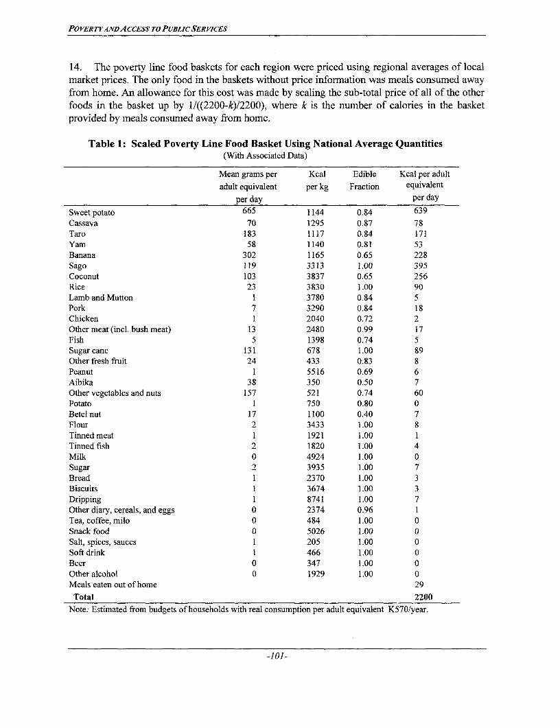
POVERTYAANDACCESS To PUBLC SER ViCES
14. The poverty line food baskets for each region were priced using regional averages of localmarket prices. The only food in the baskets without price information was meals consumed awayfrom home. An allowance for this cost was made by scaling the sub-total price of all of the otherfoods in the basket up by 1/((2200-k)/2200), where k is the number of calories in the basketprovided by meals consumed away from home.
Table 1: Scaled Poverty Line Food Basket Using National Average Quantities(With Associated Data)
Mean grams per Kcal Edible Kcal per adult
adult equivalent per kg Fraction equivalent
per day per day
Sweet potato 665 1144 0.84 639Cassava 70 1295 0.87 78Taro 183 1117 0.84 171Yam 58 1140 0.81 53Banana 302 1165 0.65 228Sago 119 3313 1.00 395Coconut 103 3837 0.65 256Rice 23 3830 1.00 90Lamb and Mutton 1 3780 0.84 5Pork 7 3290 0.84 18Chicken 1 2040 0.72 2Other meat (incl. bush meat) 13 2480 0.99 17Fish 5 1398 0.74 5Sugar cane 131 678 1.00 89Other fresh fruit 24 433 0.83 8Peanut 1 5516 0.69 6Aibika 38 350 0.50 7Other vegetables and nuts 157 521 0.74 60Potato 1 750 0.80 0Betel nut 17 1100 0.40 7Flour 2 3433 1.00 8Tinned meat 1 1921 1.00 1Tinned fish 2 1820 1.00 4Milk 0 4924 1.00 0Sugar 2 3935 1.00 7Bread 1 2370 1.00 3Biscuits 1 3674 1.00 3Dripping 1 8741 1.00 7Other diary, cereals, and eggs 0 2374 0.96 1Tea, coffee, milo 0 484 1.00 0Snack food 0 5026 1.00 0Salt, spices, sauces 1 205 1.00 0Soft drink 1 466 1.00 0Beer 0 347 1.00 0Other alcohol 0 1929 1.00 0Meals eaten out of home 29
Total 2200
Note: Estimated from budgets of households with real consumption per adult equivalent K570/year.
-101-
POVERTYAND A CCESS TO PUBLIC SER VICES
15. The region with the highest cost of buying 2200 calories per day was the NCD, where theprice was K543 per year. Households in the Highlands and Momase regions faced the lowestcost, at K307 and K250 per year. Note that these cost differences do not seem to implydifferences in the quality of the diets supplied. Consumers in the NCD would have to pay K696per year to buy the basket of foods for the Highlands region and K640 per year to buy theMomase basket. Both of these are more expensive than the actual basket bought by NCDhouseholds, and therefore the NCD basket is not revealed to be preferred to the other baskets.
16. An allowance for essential non-food items was calculated and the resulting poverty linessuggested that the highest cost of living for poor people was in the NCD, followed by the Papuanand New Guinea Islands regions. The lowest cost of living was in Momase. Setting the (austere)poverty line in the NCD equal to 100, the poverty lines in the other regions were: Papuan 74.2;Highlands 53.5; Momase 41.5; and New Guinea Islands 58.3.
17. These poverty lines, in index form, were used as deflators to convert nominal consumptioninto real consumption. This gave a group of 177 households (20 percent of the population) withreal consumption per adult equivalent less than the cut-off value of K570 per year. A new set ofregional food baskets was formed from the budgets of these households and the resulting set ofpoverty lines was calculated. These poverty lines, in index form, showed some changes from theresults of the previous iteration so the process was repeated. After the fifth iteration, the onlypoverty line changing was for the Highlands where the index number oscillated between 49.9and 50.1. These changes were sufficiently small to accept the convergence. The iterations werealso started from the values of a Tormqvist regional price index (calculated with the availableprices) and the poverty lines still converged to the same levels.
18. The poverty lines, in index form, resulting from the sixth iteration were used as the last setof deflators for defining real consumption so as to find the group of poor households whose foodbudgets would influence the poverty line food baskets. The resulting food poverty lines arereported in Table 2. The Table also reports the cost of buying each region's basket of foods at theaverage prices prevailing in every other region.
19. One problem immediately apparent in Table 2 is that two of these food poverty lines failthe revealed preference test. The basket of foods for the Momase and Papuan regions could bebought in the New Guinea Islands region for only 77 percent and 92 percent of the cost of theIslands region food basket. Hence, the poverty line for the New Guinea Islands appears to give asuperior standard of living to the poverty lines used in the Momase and Papuan regions.Similarly, the basket of foods for the Momase region can be bought in the Papuan region at only88 percent of the cost of the Papuan region basket.
-102-
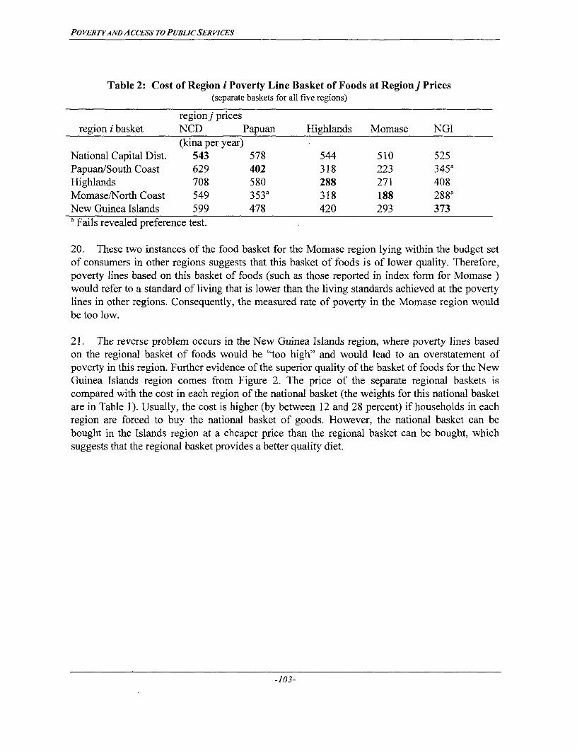
PO VERTYA ND A CCESS To PUBLIC SER VICES
Table 2: Cost of Region i Poverty Line Basket of Foods at Regionj Prices(separate baskets for all five regions)
regionj pricesregion i basket NCD Papuan Highlands Momase NGI
(kina per year)National Capital Dist. 543 578 544 510 525Papuan/South Coast 629 402 318 223 345aHighlands 708 580 288 271 408Momase/North Coast 549 353a 318 188 288aNew Guinea Islands 599 478 420 293 373a Fails revealed preference test.
20. These two instances of the food basket for the Momase region lying within the budget setof consumers in other regions suggests that this basket of foods is of lower quality. Therefore,poverty lines based on this basket of foods (such as those reported in index form for Momase )would refer to a standard of living that is lower than the living standards achieved at the povertylines in other regions. Consequently, the measured rate of poverty in the Momase region wouldbe too low.
21. The reverse problem occurs in the New Guinea Islands region, where poverty lines basedon the regional basket of foods would be "too high" and would lead to an overstatement ofpoverty in this region. Further evidence of the superior quality of the basket of foods for the NewGuinea Islands region comes from Figure 2. The price of the separate regional baskets iscompared with the cost in each region of the national basket (the weights for this national basketare in Table 1). Usually, the cost is higher (by between 12 and 28 percent) if households in eachregion are forced to buy the national basket of goods. However, the national basket can bebought in the Islands region at a cheaper price than the regional basket can be bought, whichsuggests that the regional basket provides a better quality diet.
-103-
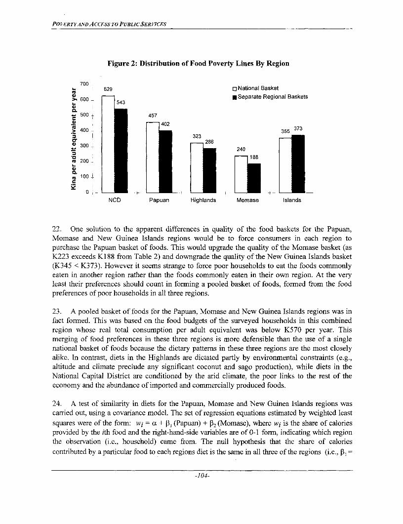
POVERTYAND A CCESS To PUBLICSER VICES
Figure 2: Distribution of Food Poverty Lines By Region
700629 [lNational Basket
> 600 _ *Separate Regional Baskets
500 457
z 400 -- 35537323
300 I n0f2_ ~~~~~~~~~~~~~~24018
Cu200
1L
100
0
NCD Papuan Highlands Momase Islands
22. One solution to the apparent differences in quality of the food baskets for the Papuan,Momase and New Guinea Islands regions would be to force consumers in each region topurchase the Papuan basket of foods. This would upgrade the quality of the Momase basket (asK223 exceeds K188 from Table 2) and downgrade the quality of the New Guinea Islands basket(K345 < K373). However it seems strange to force poor households to eat the foods commonlyeaten in another region rather than the foods commonly eaten in their own region. At the veryleast their preferences should count in forming a pooled basket of foods, formed from the foodpreferences of poor households in all three regions.
23. A pooled basket of foods for the Papuan, Momase and New Guinea Islands regions was infact formed. This was based on the food budgets of the surveyed households in this combinedregion whose real total consumption per adult equivalent was below K570 per year. Thismerging of food preferences in these three regions is more defensible than the use of a singlenational basket of foods because the dietary patterns in these three regions are the most closelyalike. In contrast, diets in the Highlands are dictated partly by environmental constraints (e.g.,altitude and climate preclude any significant coconut and sago production), while diets in theNational Capital District are conditioned by the arid climate, the poor links to the rest of theeconomy and the abundance of imported and commercially produced foods.
24. A test of similarity in diets for the Papuan, Momase and New Guinea Islands regions wascarried out, using a covariance model. The set of regression equations estimated by weighted leastsquares were of the form: wi = cx + I3 (Papuan) + P2 (Momase), where wi is the share of caloriesprovided by the ith food and the right-hand-side variables are of 0-1 form, indicating which regionthe observation (i.e., household) came from. The null hypothesis that the share of caloriescontributed by a particular food to each regions diet is the same in all three of the regions (i.e., P,1 =
-104-
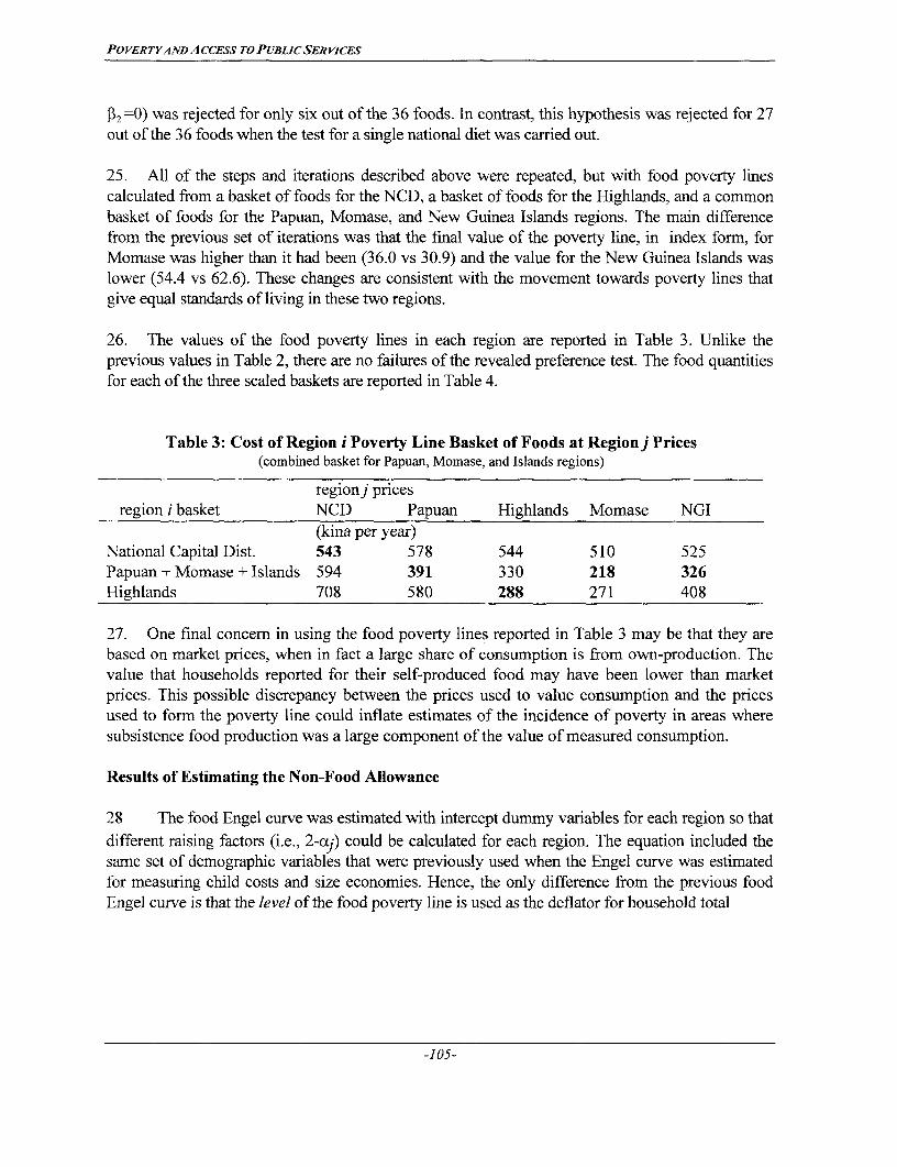
POVERTYANDACCESS TO PUBLIC SER VICES
~2 =0) was rejected for only six out of the 36 foods. In contrast, this hypothesis was rejected for 27out of the 36 foods when the test for a single national diet was carried out.
25. All of the steps and iterations described above were repeated, but with food poverty linescalculated from a basket of foods for the NCD, a basket of foods for the Highlands, and a commonbasket of foods for the Papuan, Momase, and New Guinea Islands regions. The main differencefrom the previous set of iterations was that the final value of the poverty line, in index form, forMomase was higher than it had been (36.0 vs 30.9) and the value for the New Guinea Islands waslower (54.4 vs 62.6). These changes are consistent with the movement towards poverty lines thatgive equal standards of living in these two regions.
26. The values of the food poverty lines in each region are reported in Table 3. Unlike theprevious values in Table 2, there are no failures of the revealed preference test. The food quantitiesfor each of the three scaled baskets are reported in Table 4.
Table 3: Cost of Region i Poverty Line Basket of Foods at Regionj Prices(combined basket for Papuan, Momase, and Islands regions)
regionj pricesregion i basket NCD Papuan Highlands Momase NGI
(kina per year)National Capital Dist. 543 578 544 510 525Papuan + Momase + Islands 594 391 330 218 326Highlands 708 580 288 271 408
27. One final concern in using the food poverty lines reported in Table 3 may be that they arebased on market prices, when in fact a large share of consumption is from own-production. Thevalue that households reported for their self-produced food may have been lower than marketprices. This possible discrepancy between the prices used to value consumption and the pricesused to form the poverty line could inflate estimates of the incidence of poverty in areas wheresubsistence food production was a large component of the value of measured consumption.
Results of Estimating the Non-Food Allowance
28 The food Engel curve was estimated with intercept dummy variables for each region so thatdifferent raising factors (i.e., 2-a;j) could be calculated for each region. The equation included thesame set of demographic variables that were previously used when the Engel curve was estimatedfor measuring child costs and size economies. Hence, the only difference from the previous foodEngel curve is that the level of the food poverty line is used as the deflator for household total
-105-

POVERTYAND ACCESS TO PUBLICSER VICES
Table 4: Scaled Poverty Line Food Baskets for Each RegionPapuan + Momase + New
NCD Highlands Guinea Islands
Mean grams per adult equivalent per day
Sweet potato 38 1494 272Cassava 105 70 51Taro 1 134 234Yam 0 35 87Banana 89 82 371Sago 7 4 201Coconut 66 2 143Rice 257 20 14Lamb and Mutton 30 3 0Pork 0 3 5Chicken 15 2 0Other meat (incl. bush meat) 32 24 7Fish 25 0 8Sugar cane 0 150 117Other fresh fruit 21 17 42Peanut 0 4 0Aibika 11 24 42Other Greens, vegetables, nuts 20 303 101Potato 10 2 0Betel nut 3 6 21Flour 63 0 2Tinned meat 19 0 1Tinned fish 25 2 2Milk 2 0 0Sugar 27 1 2Bread 15 0 1Biscuits 8 0 1Dripping 8 2 0Other dairy, cereals, and eggs 6 0 0Tea, coffee, milo 2 0 0Snack food I 0 0
Salt, spices, sauces 3 1 1Soft drink 29 0 0Beer 3 0 0Other alcohol 0 0 0Meals eaten out of home (Kcal) 23 44 21Note: Estimated from budgets of households with real consumption per adult equivalent < K570/year.
expenditure, x so as to scale the intercept. The weighted least squares results from estimating theequation on the full sample (rather than on just the households used to form the baskets for thefood poverty lines) were (t-statistics in ( )):
wf 0.732 - 0.052 In(I ZF) - 0 .0 08 na - O.01ncl - 0.004nc2 - 0.133 NCD + 0.033 Papuan
(2.94) (2.19) (0.22) (0.63) (5.48) (0.89)- 0.054 Highlands + 0.014 Momase R 2=0.13.
-106-
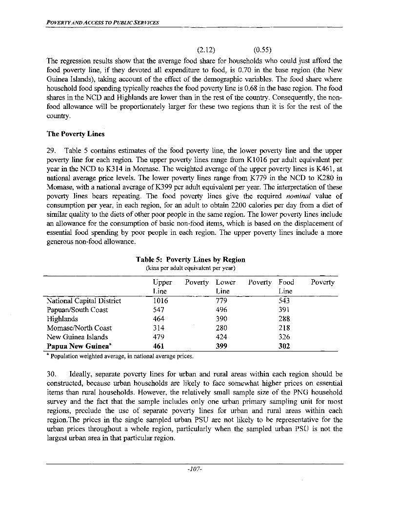
POVERTYAND ACCESS TO PUBLIC SER VICES
(2.12) (0.55)
The regression results show that the average food share for households who could just afford thefood poverty line, if they devoted all expenditure to food, is 0.70 in the base region (the NewGuinea Islands), taking account of the effect of the demographic variables. The food share wherehousehold food spending typically reaches the food poverty line is 0.68 in the base region. The foodshares in the NCD and Highlands are lower than in the rest of the country. Consequently, the non-food allowance will be proportionately larger for these two regions than it is for the rest of thecountry.
The Poverty Lines
29. Table 5 contains estimates of the food poverty line, the lower poverty line and the upperpoverty line for each region. The upper poverty lines range from K 1016 per adult equivalent peryear in the NCD to K314 in Momase. The weighted average of the upper poverty lines is K461, atnational average price levels. The lower poverty lines range from K779 in the NCD to K280 inMomase, with a national average of K399 per adult equivalent per year. The interpretation of thesepoverty lines bears repeating. The food poverty lines give the required nominal value ofconsumption per year, in each region, for an adult to obtain 2200 calories per day from a diet ofsimilar quality to the diets of other poor people in the same region. The lower poverty lines includean allowance for the consumption of basic non-food items, which is based on the displacement ofessential food spending by poor people in each region. The upper poverty lines include a moregenerous non-food allowance.
Table 5: Poverty Lines by Region(kina per adult equivalent per year)
Upper Poverty Lower Poverty Food PovertyLine Line Line
National Capital District 1016 779 543Papuan/South Coast 547 496 391Highlands 464 390 288Momase/North Coast 314 280 218New Guinea Islands 479 424 326Papua New Guineaa 461 399 302a Population weighted average, in national average prices.
30. Ideally, separate poverty lines for urban and rural areas within each region should beconstructed, because urban households are likely to face somewhat higher prices on essentialitems than rural households. However, the relatively small sample size of the PNG householdsurvey and the fact that the sample includes only one urban primary sampling unit for mostregions, preclude the use of separate poverty lines for urban and rural areas within eachregion.The prices in the single sampled urban PSU are not likely to be representative for theurban prices throughout a whole region, particularly when the sampled urban PSU is not thelargest urban area in that particular region.
-107-
POVERTYANDACCESS TO PUBLICSERVICES
31. Another alternative would be to calculate a single urban poverty line applicable to allnon-rural PSUs outside the NCD. Whether it is sensible depends on whether price variation isgreater between regions, or between rural and urban clusters within regions. To answer thisquestion, an analysis of covariance (i.e. dummy variable) model was specified, to see whether agreater contribution to the variance in cluster-level prices of important commodities came fromregions or from sectors (urban/rural). This test was done for the non-NCD regions, because thereare no rural clusters within the NCD. The regression model for the price of the ith food was:
Pricei = cx + f31 Highlands + P2 Momase + P33 New Guinea Islands + 4 Urban,
so the reference group was rural clusters in the Papuan region. The test of the hypothesis thatregional effects are unimportant was: P1=P2=P3=0, while for the hypothesis that rural/urbaneffects were unimportant it was: P4=0. The results suggested that regional effects were moreimportant for most items, and especially for the locally produced foods that supply the bulk ofthe calories in the food poverty lines (Table 6). Even some imported and commerciallydistributed items, like kerosene, showed more regional price variation than rural/urban pricevariation. These results may reflect the very limited inter-regional trade in PNG, which is causedby the difficult topography and lack of transport infrastructure. Thus, urban areas in PNG usuallyhave closer links with their rural hinterlands, than do the rural hinterlands with the rural areas ofother regions. In light of these results and given sample design constraints, this report does notdifferentiate between urban and rural poverty lines within a given region, although the sensitivityanalysis carried out in Annex 3, explores the possible effects of this omission on the povertymeasures for PNG.
-108-

POVERTYANDACCESS TO PUBLIC SER VICES
Table 6: Determinants of Regional and Sectoral Price Variations
Regional effects = 0 Urban/rural effects = 0F-value p-value F-value p-value
Sweet potato 23.39 0.00 5.57 0.03Betelnut 21.16 0.00 1.40 0.25Sugarcane 6.76 0.00 3.53 0.07Banana 6.48 0.00 2.72 0.11Cassava 6.46 0.00 2.56 0.13Kerosene 6.02 0.00 4.79 0.04Taro 5.11 0.00 8.37 0.02Flour 4.60 0.00 35.57 0.00Rice 4.50 0.00 44.27 0.00Coconut 4.31 0.02 0.08 0.79Aibika 4.24 0.00 1.16 0.29Canned meat 3.73 0.01 7.86 0.01Petrol 2.55 0.07 1.92 0.17Yams 2.36 0.10 0.69 0.42Dripping 1.07 0.37 0.27 0.61Sugar 2.58 0.06 35.91 0.00Coarse-cut tobacco 2.28 0.09 20.74 0.00Canned fish 2.56 0.06 11.63 0.00Sago 1.22 0.34 1.61 0.23Tea 0.70 0.56 1.05 0.31
-109-
POVERTYANDACCESS TO PUBLICSERVICES
ANNEX 11124: EFFECT OF USING SAMPLING UNIT SPECIFIC PRICES ANDURBAN/RURAL PRICE DIFFERENTIALS IN POVERTY LINES
1. The poverty measurements in chapter 1 of this report rely on poverty lines that are set forjust five regions: the Papuan/South Coast, the Highlands, the Momase/North Coast, the NewGuinea Islands, and the National Capital District. Arithmetic averages of food prices in eachregion were used to calculate the cost of buying the poverty line basket of foods, which anchorsthe poverty lines. It is likely that these regional average prices overstate the cost of buying thebasket of foods in some Census Units within each region, while understating it for others.Measured poverty will be too high in CUs where regional average prices overstate the cost of thebasket of foods because these same (high) prices are not used for valuing food consumption.Hence, the value of some households' consumption will be above the poverty line if that line ispriced using local (i.e., Census Unit) prices, but below the poverty line if regional average pricesare used. This problem occurs even if consumption is valued using local market prices, ratherthan respondent-Teported values. Bias in the opposite direction (measured poverty too low) willoccur in CUs where regional average prices understate the local cost of the poverty line basket offoods.
2. At first glance, it would seem that there is no net effect of using regional average pricesbecause the overstatement of poverty in some CUs within the region is cancelled out by theunderstatement in others. This would be true if the distribution of food prices within each regionwas symmetric, with the mean equalling the median (e.g., a Normal distribution). However, thereis evidence that the within-region distribution of prices is positively skewed, with the meanexceeding the median. For example, the hypothesis that the distribution of surveyed sweet potatoprices across Census Units in the Highlands comes from a Normal distribution is rejected(p<O.O1), while the hypothesis of log-normality is not rejected (p<0.50). A consequence of thelack of nornality is that only 39 percent of the surveyed CUs in the Highlands have sweet potatoprices above the regional average price. Hence, the regional average price for sweet potatooverstates the cost of the main component of the Highlands food poverty line more often than itunderstates it. A similar pattern holds for three-quarters of the combinations of regions andfoods, so there is a high likelihood that the net effect of using regional average prices is tooverstate poverty.
3. The obvious solution to the problem caused by using regional average prices is tocalculate the cost of the food poverty line separately for each Census Unit. This was not done inchapter 1 of the report because the design of the price survey meant there was no way todistinguish between spatial and temporal components of price differences. For example, two riceprices observed by the survey might have been K1.00/kg for a CU in Eastern Highlands provincein January and Kl .1 0/kg for a CU in the Western Highlands province in March. There is no wayto know if this is a spatial difference, which always holds in these locations, or just a temporaldifference due to the general movement in prices between January and March. The spatial price
24 Based on Gibson, J. and S. Rozelle, (1998)
-110-
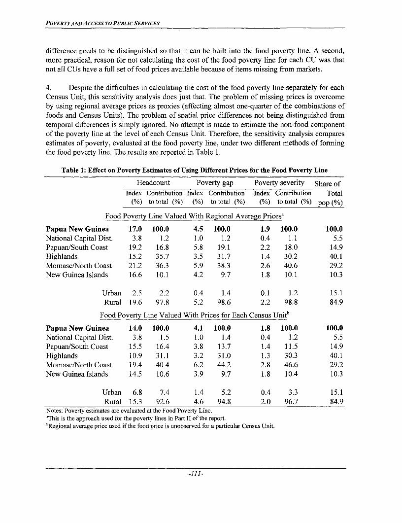
POVERTYANDACCESS To PUBLICSERVICES
difference needs to be distinguished so that it can be built into the food poverty line. A second,more practical, reason for not calculating the cost of the food poverty line for each CU was thatnot all CUs have a full set of food prices available because of items missing from markets.
4. Despite the difficulties in calculating the cost of the food poverty line separately for eachCensus Unit, this sensitivity analysis does just that. The problem of missing prices is overcomeby using regional average prices as proxies (affecting almost one-quarter of the combinations offoods and Census Units). The problem of spatial price differences not being distinguished fromtemporal differences is simply ignored. No attempt is made to estimate the non-food componentof the poverty line at the level of each Census Unit. Therefore, the sensitivity analysis comparesestimates of poverty, evaluated at the food poverty line, under two different methods of formingthe food poverty line. The results are reported in Table 1.
Table 1: Effect on Poverty Estimates of Using Different Prices for the Food Poverty Line
Headcount Poverty gap Poverty severity Share of
Index Contribution Index Contribution Index Contribution Total(%) tototal (%) (%) tototal (%) (%) to total (%) pop(%)
Food Poverty Line Valued With Regional Average Pricesa
Papua New Guinea 17.0 100.0 4.5 100.0 1.9 100.0 100.0National Capital Dist. 3.8 1.2 1.0 1.2 0.4 1.1 5.5Papuan/South Coast 19.2 16.8 5.8 19.1 2.2 18.0 14.9Highlands 15.2 35.7 3.5 31.7 1.4 30.2 40.1Momase/North Coast 21.2 36.3 5.9 38.3 2.6 40.6 29.2New Guinea Islands 16.6 10.1 4.2 9.7 1.8 10.1 10.3
Urban 2.5 2.2 0.4 1.4 0.1 1.2 15.1Rural 19.6 97.8 5.2 98.6 2.2 98.8 84.9
Food Poverty Line Valued With Prices for Each Census Unitb
Papua New Guinea 14.0 100.0 4.1 100.0 1.8 100.0 100.0National Capital Dist. 3.8 1.5 1.0 1.4 0.4 1.2 5.5Papuan/South Coast 15.5 16.4 3.8 13.7 1.4 11.5 14.9Highlands 10.9 31.1 3.2 31.0 1.3 30.3 40.1Momase/North Coast 19.4 40.4 6.2 44.2 2.8 46.6 29.2New Guinea Islands 14.5 10.6 3.9 9.7 1.8 10.4 10.3
Urban 6.8 7.4 1.4 5.2 0.4 3.3 15.1Rural 15.3 92.6 4.6 94.8 2.0 96.7 84.9
Notes: Poverty estimates are evaluated at the Food Poverty Line.aThis is the approach used for the poverty lines in Part II of the report.bRegional average price used if the food price is unobserved for a particular Census Unit.
-111-
POVERTYAND ACCESS TO PUBLICSERVICES
5. Measured poverty is reduced when the food poverty line is calculated separately for eachCensus Unit (Table 1). The national estimate of the headcount index is reduced by aboutone-sixth, and the poverty gap index by about one-tenth. The Highlands is the region with thebiggest fall in measured poverty when the food poverty line is calculated separately for eachCensus Unit rather than for the region as a whole. The National Capital District and the NewGuinea Islands have the smallest fall in measured poverty when this change is made. It appearsthat regional average prices understate the cost of the food poverty line in urban areas becausepoverty estimates for urban areas rise once the food poverty line is calculated for each CensusUnit. In contrast, the poverty estimates for rural areas fall when the food poverty line iscalculated for each Census Unit. However, these changes are not sufficient to overturn theconclusion that the poverty rate in rural areas is much higher than it is in urban areas.
6. It seems apparent from the resuits in Table 1 that measured poverty rates can be reducedby increasing the number of spatial points where poverty lines are set. A further example of thiseffect can be found by disaggregating the poverty lines for the Momase region into two sectors:rural and urban. Attention is paid just to this region because it has the largest number of urbanCensus Units in the sample (four). The poverty lines for the urban and rural sectors are based ona common basket of foods, (which is used for the Papuan and New Guinea Islands regions aswell) but average food prices are calculated separately for each sector. A separate non-foodallowance is also calculated for each of the two sectors, based on the intercept dummies in thefood Engel curve. Notably, the coefficient on expenditure in the food Engel curve was changedby the presence of the intercept dummies for each sector within Momase, and this affected theestimated non-food allowances for all of the other regions. Table 2 reports the full set of povertylines for all regions when a separate urban and rural sector is allowed in the Momase region.These poverty lines can be compared with those in Table 1.5 of chapter 1, where urban and ruralsectors in the Momase region are combined.
Table 2: Poverty Lines With Urban and Rural Sectors Split For the Momase Region
Upper Poverty Lower Poverty Food PovertyLine Line Line
National Capital District 1047 792 543Papuan/South Coast 552 500 391Highlands 468 394 288Momase: Urban 545 429 301
Rural 261 239 189New Guinea Islands 482 427 326
7. The poverty line in the urban sector of Momase is approximately twice as high as the ruralpoverty line (Table 2). Consequently, a single regional poverty line that is the average of thehigh-cost urban sector and the low-cost rural sector will understate poverty in the urban sectorand overstate poverty in the rural sector of this region. To see whether these opposite effectscancel each other out, the regional poverty profile was recalculated using the poverty lines
-112-
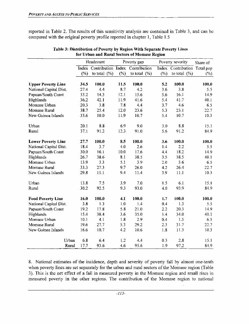
POVERTYAND ACCESS TO PUBLIC SER VICES
reported in Table 2. The results of this sensitivity analysis are contained in Table 3, and can becompared with the original poverty profile reported in chapter 1, Table 1.5
Table 3: Distribution of Poverty by Region With Separate Poverty Linesfor Urban and Rural Sectors of Momase Region
Headcount Poverty gap Poverty severity Share ofIndex Contribution Index Contribution Index Contribution Total pop
(%) to total (%) (%) to total (%) (%) to total (%) (%)
Upper Poverty Line 34.5 100.0 11.5 100.0 5.2 100.0 100.0National Capital Dist. 27.4 4.4 8.7 4.2 3.6 3.8 5.5Papuan/South Coast 33.2 14.3 12.1 15.6 5.6 16.1 14.9Highlands 36.2 42.1 11.9 41.6 5.4 41.7 40.1Momase Urban 20.3 3.8 7.8 4.4 3.7 4.6 6.5Momase Rural 38.7 25.4 12.0 23.6 5.3 23.1 22.7New Guinea Islands 33.6 10.0 11.9 10.7 5.4 10.7 10.3
Urban 20.1 8.8 6.9 9.0 3.0 8.8 15.1Rural 37.1 91.2 12.3 91.0 5.6 91.2 84.9
Lower Poverty Line 27.7 100.0 8.5 100.0 3.6 100.0 100.0National Capital Dist. 18.4 3.7 4.0 2.6 1.4 2.2 5.5Papuan/South Coast 30.0 16.1 10.0 17.6 4.4 18.2 14.9Highlands 26.7 38.6 8.1 38.5 3.5 38.5 40.1Momase Urban 13.9 3.3 5.1 3.9 2.0 3.6 6.5Momase Rural 33.3 27.3 9.7 26.0 4.2 26.4 22.7New Guinea Islands 29.8 11.1 9.4 11.4 3.9 11.1 10.3
Urban 13.8 7.5 3.9 7.0 1.5 6.1 15.1Rural 30.2 92.5 9.3 93.0 4.0 93.9 84.9
Food Poverty Line 16.0 100.0 4.1 100.0 1.7 100.0 100.0National Capital Dist. 3.8 1.3 1.0 1.4 0.4 1.3 5.5Papuan/South Coast 19.2 17.8 5.8 21.0 2.2 20.3 14.9Highlands 15.4 38.4 3.6 35.0 1.4 34.0 40.1Momase Urban 10.1 4.1 1.8 2.9 0.4 1.5 6.5Momase Rural 19.6 27.7 5.3 29.2 2.3 31.7 22.7New Guinea Islands 16.6 10.7 4.2 10.6 1.8 11.3 10.3
Urban 6.8 6.4 1.2 4.4 0.3 2.8 15.1Rural 17.7 93.6 4.6 95.6 1.9 97.2 84.9
8. National estimates of the incidence, depth and severity of poverty fall by almost one-tenthwhen poverty lines are set separately for the urban and rural sectors of the Momase region (Table3). This is the net effect of a fall in measured poverty in the Momase region and small rises inmeasured poverty in the other regions. The contribution of the Momase region to national
-I113-
POVERTY AND ACCESS TO PUBLIC SER ViCES
poverty (at the Upper Poverty Line) falls from 35.5 percent to 29.2 percent, when a singleregional poverty line is replaced with separate poverty lines for the urban and rural sectors. It isclear that the overstatement of rural poverty caused by the use of a single regional poverty linefor Momase is not fully cancelled out by the understatement of urban poverty. Finally, thenational estimates of food poverty in Table 3 show that separate poverty lines for the urban andrural sectors of Momase have less effect than calculating the cost of the poverty line separatelyfor each Census Unit. The national estimate of food poverty is 16 percent when poverty lines areset separately for the urban and rural sectors of Momase, but only 14 percent when the cost of thefood poverty line is calculated separately for each CU.
9. The common feature of the sensitivity analyses in Table 2 and Table 3 is that they increasethe number of points where poverty lines are set. The fall in poverty estimates following thesechanges suggests that temporal poverty comparisons may be affected by the choice of how manysectors to set separate poverty lines for. If the next survey has more primary sampling units(CUs) it should be possible to set poverty lines either for smaller areas (e.g., Provinces) or elseseparately for urban and rural sectors within regions. The next survey might also revisit surveyedCensus Units several times over the course of the year, so that the spatial component of pricedifferences can be separated from the temporal component. This would enable the cost of thepoverty lines to be calculated separately for each Census Unit. Both of these changes in thedesign of the next survey would tend to produce lower estimates of poverty than would areplication of the current survey design. Therefore, when analysts of the next survey wish tomake temporal poverty comparisons, they should base those comparisons on poverty lines thatare set for the same five regions used by this survey. But when analysts of the next survey wantto make the most accurate estimates of current poverty they should calculate poverty lines for asmany spatial points as possible.
-114-
POVERTY AND AccEss TO PUBLICSER VICES
ANNEX IV: DETERMINANTS OF CHILD GROWTHL5
I. There are indications that a woman's education may have a direct bearing on the healthand overall welfare of her children. As well as the usual higher income resulting from extraeducation, educated mothers are also more likely to have fewer and healthier children. This claimis relevant to Papua New Guinea because of (i) the high rate of infant and child mortality, and (ii)the substantial gap in education levels that exists between men and women. Therefore, it isworthwhile testing whether improvements in child health are likely if Papua New Guineainvested more heavily in girls' education.
2. There are several pathways through which education can affect child health. First, there isan income pathway, where education may help to increase parent's incomes, allowing extraspending on food and health care for the child. Second, there is an efficiency pathway, whereeducation may improve understanding of health and nutrition so that even with a given income ahousehold is able to produce taller, heavier and healthier children. Third, there is a power pathway,where increasing the education of women may increase their say in household decision-making. Ifwomen have greater concern for children's growth and nutrition than men do, their increased saymay lead to more resources being allocated to the children.
3. The effect of mother's education on child health was analysed by estimating a multivariatemodel of the risk of a child being stunted (height-for-age more than two standard deviations belowthe median of the reference population). The main reason for choosing stunting as the indicator ofinadequate child health was that it is the best long-run anthropometric indicator. Low height-for-agereflects chronic malnutrition due to the accumulated effect of extended periods of inadequatefood intake and past episodes of infection and sickness.
4. There is a high correlation between the education level of husbands and wives, so theresearch design has to ensure that the coefficient on mother's education in the child stuntingmodel is not in fact measuring something else. The estimation strategy was to first use a variablemeasuring the average years of education of the child's parents. This variable was thendisaggregated into years of education for the mother and years of education for the father.Additional variables, whose (excluded) effects might be picked up by the mother's educationvariable were then added to the model.
5. The model of child stunting also had a number of control variables. The household surveyshowed that the incidence of stunting varies considerably, according to the age of the child and,especially, the region of the country. Variables controlling for age and region were thereforeincluded in the equation predicting whether or not the child was stunted. No gender difference instunting rates was found, either unconditionally (tz=0.63) or conditioning on other variables
25 This annex is based on a report by John Gibson and Scott Rozelle entitled "Results of the Household SurveyComponent of the 1996 Poverty Assessment for Papua New Guinea".
-1 15-
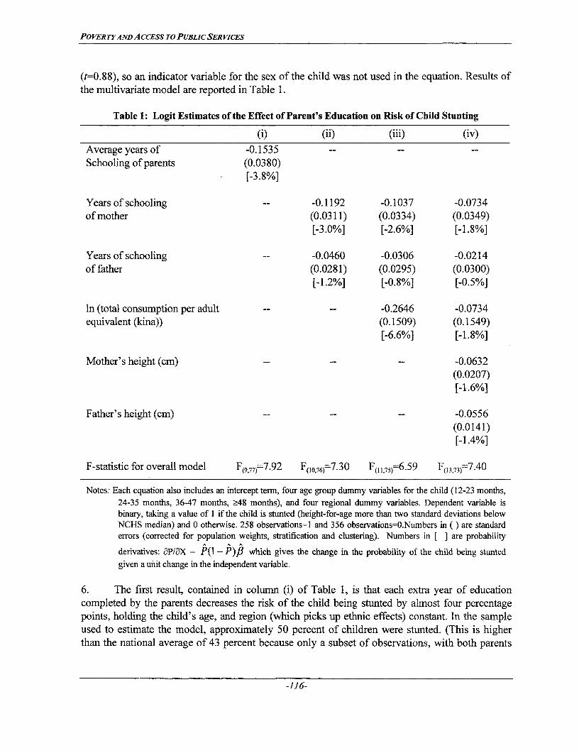
POVERTYAND ACCESS TO PUBLICSERVICES
(t=0.88), so an indicator variable for the sex of the child was not used in the equation. Results ofthe multivariate model are reported in Table 1.
Table 1: Logit Estimates of the Effect of Parent's Education on Risk of Child Stunting
(i) (ii) (iii) (iv)
Average years of -0.1535 -- -- --Schooling of parents (0.0380)
[-3.8%]
Years of schooling -- -0.1192 -0.1037 -0.0734of mother (0.0311) (0.0334) (0.0349)
[-3.0%] [-2.6%] [-1.8%]
Years of schooling -- -0.0460 -0.0306 -0.0214of father (0.0281) (0.0295) (0.0300)
[-1.2%] [-0.8%] [-0.5%]
In (total consumption per adult -- -- -0.2646 -0.0734equivalent (kina)) (0.1509) (0.1549)
[-6.6%] [-1.8%]
Mother's height (cm) -- -- -- -0.0632(0.0207)[-1.6%]
Father's height (cm) -- -- -- -0.0556(0.0141)[- 1.4%]
F-statistic for overall model F(9,77)7.92 F(10 76)=7.30 F( 1,75)-6.59 F(13,73 )=7.40
Notes: Each equation also includes an intercept term, four age group dummy variables for the child (12-23 months,
24-35 months, 36-47 months, >48 months), and four regional dummy variables. Dependent variable isbinary, taking a value of I if the child is stunted (height-for-age more than two standard deviations belowNCHS median) and 0 otherwise. 258 observations=1 and 356 observations=O.Numbers in ( ) are standarderrors (corrected for population weights, stratification and clustering). Numbers in [ ] are probability
derivatives: aPlaX = P(1 - P)fi which gives the change in the probability of the child being stunted
given a unit change in the independent variable.
6. The first result, contained in column (i) of Table 1, is that each extra year of educationcompleted by the parents decreases the risk of the child being stunted by almost four percentagepoints, holding the child's age, and region (which picks up ethnic effects) constant. In the sampleused to estimate the model, approximately 50 percent of children were stunted. (This is higherthan the national average of 43 percent because only a subset of observations, with both parents
-116-

POVERTYAND ACCESS TO PUBLUCSER VICES
in the household and having full data available, were used for the model, N=614.) Thus, forchildren of the same age group in the same region, having parents who had both completedcommunity school (six years of education) would almost halve the risk of being stunted, comparedwith children whose parents had never attended school.
7. The results in column (ii) show that most of this effect comes from the education of women,rather than of men. An extra year of education for the mother reduces the risk of child stunting bythree percentage points. This effect is three times larger than the effect of an extra year of educationfor the father. This suggests that efforts to especially increase the education gained by women mayhave big payoffs. The adult women in the sample had two years less education, on average, than themen (2.9 years versus 5.0 years). Closing this schooling gap could reduce the proportion of childrenwho are stunted by six percentage points. Not only is the payoff to men's schooling -- in terms ofimproved child health -- lower, it is also less precisely estimated. In fact, the hypothesis thatfather's education has no effect on the risk of stunting would not be rejected at usual confidencelevels (p=O.11).
8. Are these findings about the more powerful effect of mother's education on child healthrobust? The first test is to add a variable measuring the economic resources of the household. Thegender gap in adult schooling levels falls as household income rises, so any excluded effect ofhousehold economic resources on child stunting may bias the coefficient on mother's education.Results of the test are shown in column (iii), with the logarithm of real consumption per adultequivalent used to measure household economic resources. There is a slight fall in the size andstatistical significance of the coefficients on both parents education, but mother's schooling stillappears three times more effective than father's schooling (the statistical significance of thedifference is also unchanged from the results in column (ii)).
9. The significant effect of mother's education on stunting probabilities, even when householdeconomic resources are controlled for, suggests that most of the effect of education on child growthdoes not come through the income pathway. Instead, it may work either through the efficiencypathway, with mother's education most effective because they spend more time caring for childrenthan fathers do, or through the power pathway, with children benefiting from the bigger say thateducated women have in household decision-making.
10. A second robustness test of robustness is to add variables that measure parental health,because the coefficients on schooling may be picking up excluded effects of, especially, maternalhealth. Results of this test are shown in column (iv), with parental height used as a proxy for health(height will also pick up genetic and ethnic effects). Parental height is highly relevant to the risk ofa child being stunted, but the difference between the effect of mother's height and father's height isnot significant (p=0.71). Adding parental height to the model has most impact on the measuredeffect of household economic resources: the coefficient on consumption per adult-equivalent fallsto one-quarter its previous value and the null hypothesis that economic resources have no effect onthe risk of stunting is not rejected (p=0.74). The lower coefficients on schooling in column (iv)suggest that the previous results were picking up some excluded effects of maternal health but even
-117-
POVERTYANDACCESS TO PUBLICSERVICES
with that addition to the model, mother's education still exerts a powerful effect on the risk of childstunting.
11. The significant effects of mother's height and mother's education on stuntingprobabilities indicates that there is a long-run, intergenerational, effect of women's education onchild health. Educating the current generation of girls will reduce the risk that their own childrenare stunted. Those children are likely to become taller adults which will then reduce the risk ofthe next generation of children being stunted.
12. In summary, the results of this analysis suggest a role for public action because privatechoices are likely to lead to less women's education than is socially desirable. When parents choosewhether to send their daughter to school they are probably unaware of the impact that this choicehas on the health of their yet-to-be-born grandchildren. This "external" effect may lead parents tounder-invest in the schooling of their daughters.
-1 18-

POVERTYAND ACCESS To PUBLICSERVICES
ANNEX V: DECOMPOSING THE GENDER GAP IN PARIMARY SCHOOLENROLMENTS IN PAPUA NEW GUINEA26
I. Introduction
1. Results from the educational module of the 1996 Papua New Guinea Household Surveyshow that the country is a long way from achieving universal primary education. Over one-thirdof children between age 6 and age 20 years have never been to school and even at the age whenenrolments peak (10-12 years), less than 70 percent of children are in school. There is also alarge gender gap in school enrolments, with female enrolment rates declining from 68 percent atage 1 I to 45 percent at age 14 years and 13 percent by age 18. In contrast, 60 percent of malesare still enrolled at age 14 and 26 percent are enrolled at age 18.27
2. The success at enrolling children in school varies widely between regions. Overallenrolment rates are highest, and the gender gaps are smallest, in the NCD and the New GuineaIslands. The overall enrolment rate is lowest in the Highlands, at less than two-thirds of the ratein the NCD and Islands regions, while the gender gap is largest in the Momase region with girlsonly two-thirds as likely as boys to be in the appropriate level of school.
3. A regression model of the probability of a child being enrolled in Community School(i.e., Grades 1-6) is used in this paper to gain some insights into the causes of this poor enrolmentrecord.28 This model may help to explain whether the gap in enrolments between boys and girlsand between regions is simply a function of variation in observable characteristics. Thisknowledge can help to determine whether it is more appropriate to use geographical, householdor individual (i.e., gender) characteristics for targeting interventions designed to raise enrolmentrates.
II. Data and Model Specification
4. Data used in this paper come from the 1996 PNG Household Survey. The survey startedwhile students were still on school holidays, so all questions about current enrolments referred tothe previous (1995) year. The sample selected for this analysis is based on all members ofrespondent households aged between 7-17 years in 1995, who had not completed CommunitySchool (i.e., Grade 6) before the 1995 school year. This wide age interval is needed becauseover-age enrolment is a common problem in Papua New Guinea (e.g., 20 percent of the 17 year
26 This annex is based on Gibson, John, (1999f), "Decomposing The Gender Gap in Primary School Enrolments inPapua New Guinea", Mimeo, prepared for the Poverty Assessment.
27 These enrolment rates are age-specific, and show the proportion of children of a given age attending any level ofschool.
28 The method of analysis is similar to that recently used by Handa (1996) and Ravallion and Wodon (1999).
-119-

POVERTYAND ACCESS TO PUBLIC SER VICES
olds in our sample were still attending Community School). These selection criteria gave asample of 1528. The model seeks to explain the enrolment status of children, as captured by thequestion "Did you go to school in 1995?" A total of 755 children in this sample (correspondingto a population-weighted proportion of 0.452) attended school in 1995.
5. A wide range of variables measuring the potential determinants of enrolments are availablefrom the survey and these are described under the following four headings: child characteristics,household characteristics, community characteristics and regional fixed effects.
Child characteristics: a linear and quadratic term in the child's age and an indicator variable forwhether the child's parent is the head of the household.
Household characteristics: (log) household size, the share of young children (age 0-6), olderchildren (age 7-14), and prime-age adults (age 15-50), plus a binary variable for female-headedhouseholds are included. It is difficult to identify the parents of many of the children in thesample, because household members were classified only by their relationship to the householdhead. So in place of the usual variables of mother's and father's education levels, the householdaverages of the completed school years for adult males and adult females are used. Thesevariables should still capture the potential demand by educated adults for child enrolmentsbecause there is evidence of considerable educational spillovers within households in Papua NewGuinea (Gibson, 1999).
Community characteristics: the travelling time to the nearest community school using thetransport method most typically used by students within the PSU.
Regional fixed effects: Dummy variables for the regions (n=5) used in descriptive analysis. Ifthese variables remain significant after controlling for the other observables it may suggest thatgeographical targeting is a sensible basis for programs that seek to raise school enrolment rates.
MII. Results and Interpretation
6. Table 1 reports the means and standard deviations of the variables, disaggregated by sex.Table 2 reports probit estimates of the enrolment equations. To test whether estimating the modelseparately for boys and girls was appropriate, a dummy variable for the sex of the child wasinteracted with all slope variables and the model was re-estimated on the pooled sample. The testthat the male intercept dummy plus all 16 of the interacted slope dummy variables were jointlyzero was rejected at the p<0.08 level (F(17 89)l1.69). Although one might pool the data on thebasis of this result, it is worth emphasising that the hypothesis test used is a very conservativeone, with degrees of freedom based on the number of clusters rather than the number ofobservations.2 9 Thus, the estimation of separate models for the enrolments of boys and girls isappropriate.
29 If the test is based on the number of observations, while still controlling for sampling weights and clustering, thepooling assumption is rejected at the p<O.02 level (X2
(l7)=3 1.8).
-120-

POVERTYA.ND ACCESS To PUBLICSERVICES
Table 1: Variable Means (Standard Deviations) by SexFull Sample Girls Boys
Child characteristicsEnrolled in school in 1995? 0.452 0.425 0.475
(0.50) (0.49) (0.50)Age ofthe child 12.125 12.187 12.073
(2.96) (2.99) (2.94)Child of household head 0.777 0.770 0.782
(0.42) (0.42) (0.41)Household characteristicslog expenditure per adult equiv.a 6.321 6.315 6.326
(0.77) (0.80) (0.74)log household size 1.973 1.961 1.983
(0.43) (0.44) (0.42)Share of children 0-6 0.153 0.150 0.156
(0.13) (0.13) (0.13)Share of children 7-14 0.308 0.303 0.312
(0.14) (0.14) (0.14)Share of adults <51 0.478 0.478 0.478
(0.17) (0.18) (0.17)Female household head 0.072 0.068 0.075
(0.26) (0.25) (0.26)Men's years of school 4.032 4.038 4.027
(3.60) (3.81) (3.42)Women's years of school 2.609 2.646 2.578
(2.94) (2.92) (2.95)Community characteristicsTravel time to school 59.282 60.961 57.886
(92.37) (98.68) (86.80)NCD 0.040 0.042 0.038
(0.20) (0.20) (0.19)Papuan/South Coast 0.135 0.140 0.130
(0.34) (0.35) (0.34)Highlands 0.440 0.418 0.457
(0.50) (0.49) (0.50)Momase/North Coast 0.291 0.292 0.290
(0.45) (0.45) (0.45)Observations 1528 700 828
Notes: Means and standard deviations are calculated using household sampling weights.
a In real, national average prices, where the regional poverty lines are used to deflate nominal expenditures. Theadult equivalence scale counts children age 0-6 as 0.5 adults and everyone else as 1.0.
7. In general, the results in the first two columns of Table 2 suggest that the probability ofbeing in school is significantly affected by the age of the child, by household economicresources, by the education level of adults, and by the distance to the nearest Community School.However, the relationship of the child to the household head, and the size, demographiccomposition and female headship of the household are less statistically significant explanatoryvariables.
-121-

POVERTYAND ACCESS TO PUBLIC SER VICES
Table 2: Probit Coefficients for Enrolment in Community School by Sex
Exogenous Expenditure Endogenous ExpenditureGirls Boys Girls Boys
Child characteristicsAge of the child 1.404 1.529 1.407 1.521
(6.17)*** (8.06)*** (6.24)*** (8.00)***(Age of child)2 -0.053 -0.057 -0.053 -0.057
(5.93)*** (7.79)*** (6.02)*** (7.71)***Child of household head 0.256 0.033 0.251 0.048
(1.51) (0.21) (1.47) (0.30)Household characteristicslog expenditure per ad. equiv. 0.199 0.169 0.139 0.341
(2.54)** (2.11)** (0.58) (1.78)*First stage residuals 0.074 -0.203
(0.24) (1.07)log household size 0.103 0.313 0.074 0.392
(0.62) (1.89)* (0.40) (2.11)**Share of children 0-6 -0.328 -0.046 -0.321 -0.006
(0.47) (0.06) (0.47) (0.01)Share of children 7-14 -0.069 -0.393 -0.096 -0.261
(0.09) (0.56) (0.13) (0.36)Share of adults <51 -0.786 -1.095 -0.790 -1.020
(1.30) (1.69)* (1.30) (1.54)Female household head -0.055 0.326 -0.062 0.348
(0.20) (1.34) (0.22) (1.48)Men's years of school 0.082 0.056 0.085 0.046
(3.81)*** (2.51)** (3.53)*** (1.89)*Women's years of school 0.089 0.018 0.092 0.008
(3.09)*** (0.64) (2.74)*** (0.25)Community characteristicsTravel time to school -0.007 -0.007 -0.007 -0.006
(3.63)*** (3.14)*** (3.55)*** (3.08)***NCD -0.614 0.170 -0.603 0.117
(2.29)** (0.62) (2.24)** (0.44)Papua -0.600 -0.072 -0.583 -0.116
(2.04)** (0.25) (1.92)* (0.40)Highlds -0.526 -0.243 -0.500 -0.324
(2.03)** (1.13) (1.70)* (1.41)Momase -0.552 0.117 -0.540 0.075
(2.09)** (0.47) (1.98)* (0.30)Constant -10.028 -10.702 -9.627 -11.896
(5.83)*** (7.10)*** (3.79)*** (5.75)***Zero slopes testa F(16S7) 13.13*** 7.50*** 12.33*** 7.03***Observations 700 828 700 828
Notes: Results corrected for the effect of clustering, sampling weights and stratification. Absolute value of t-statistics in ( ).
* significant at 10 percent level; ** significant at 5 percent level; *** significant at I percent level.
aThis is an adjusted Wald (iW) test: (d - k + l/kd) W-F(k, d - k + 1), where d is the number of clusters minusthe number of strata (102), and k is the number of slope variables (StataCorp, 1999).
-122-
POVERTYAND ACCESS To PUBLIC SER VICES
8. There are several differences between the equations for boys and girls which should behighlighted. First, adult education has a much larger impact on the enrolment of girls than ofboys, and in fact there is no significant effect of adult women's school years on the probability ofa boy being in school. Second, the coefficients on the regional fixed effects show that theobserved characteristics of children, households and communities can account for all regionaldifferences in the enrolment rates of boys but not of girls. In particular, even after controlling forobservables, all regions lag significantly behind the New Guinea Islands in the enrolment ofgirls. Thus there may be some need to transfer policies and institutions that have worked tofavour female enrolments in the Islands region to the rest of PNG.
9. One potential problem with the results in the first two columns of Table 2 is that totalexpenditures per adult equivalent is potentially endogenous in a regression explaining humancapital investments. To see if the results are sensitive to this effect, the Rivers and Vuong (1988)two-step estimator was used, with the residuals from a first-stage OLS regression predicting (log)expenditures per adult equivalent included in the probit equation alongside the expenditurevariable.30 A t-test on the added residual acts as a test of endogeneity. The results in the last twocolumns of Table 2 show that endogeneity bias is not apparent in either of the equations becausethe t-statistics on the first-stage residuals are always statistically insignificant. Therefore theestimates that treat expenditures as exogenous are used for the remainder of the paper.
10. The gender gap in enrolments that is predicted by the probit equation can be decomposedfollowing a method used by Even and Macpherson (1993):
GAP = P(Xm ft.)- P(X, fXj) = 0.4768 -0.4250 = 0.0518
where Xi is the vector of observed characteristics (including household and community effects)for the child of sex i, and ,Bi is the corresponding vector of coefficients. This gap can bedecomposed into an explained portion, due to differences in characteristics (i.e., differences inthe Xi vectors) by comparing the enrolment rate that girls would have if they had the observedcharacteristics of the boys in the sample with the enrolment rate predicted from their owncharacteristics:
EXPLAINED GAP = P(Xm,M /f )-P(Xj, /f) = 0.4188-0.4250 =-0.0062.
11. Thus, the enrolment rate for girls would be slightly lower if they were to have thecharacteristics of the boys in the sample, so differences in observable characteristics are not
30 In addition to the exogenous variables in Table AV.2, the instruments in the first stage regression includedvariables measuring characteristics of the dwelling (floor area, number of rooms and whether the roof wasiron), characteristics of the household head(age, literacy, years of schooling and whether working for wages),and indicator variables for the ownership of agricultural capital goods and pigs (the main form of wealth). TheR2 from the first stage regression was 0.37 and the F-test for excluding the instruments was F(997)=6.96 whichis significant at the p<O.OI level.
-123-
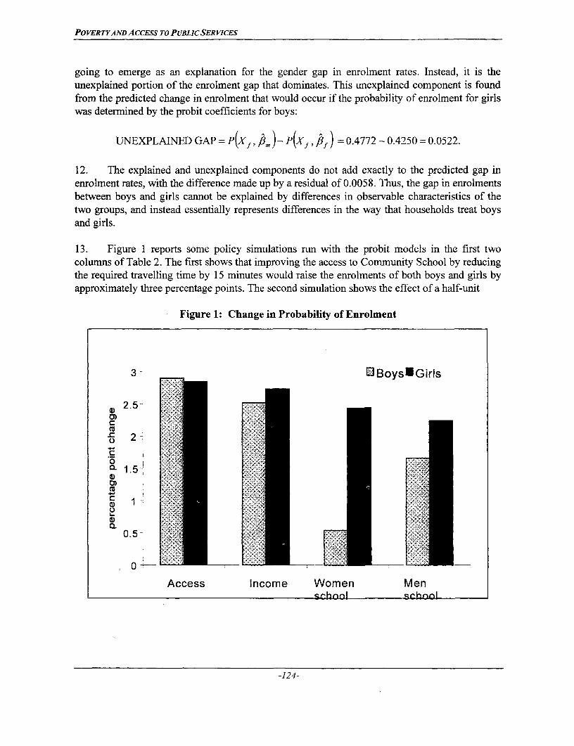
POVERTYAND ACCESS TO PUBLICSER VICES
going to emerge as an explanation for the gender gap in enrolment rates. Instead, it is theunexplained portion of the enrolment gap that dominates. This unexplained component is foundfrom the predicted change in enrolment that would occur if the probability of enrolment for girlswas determined by the probit coefficients for boys:
UNEXPLAINED GAP = P(X,, im )- P(X,, ) = 0.4772 - 0.4250 = 0.0522.
12. The explained and unexplained components do not add exactly to the predicted gap inenrolment rates, with the difference made up by a residual of 0.005 8. Thus, the gap in enrolmentsbetween boys and girls cannot be explained by differences in observable characteristics of thetwo groups, and instead essentially represents differences in the way that households treat boysand girls.
13. Figure 1 reports some policy simulations run with the probit models in the first twocolumns of Table 2. The first shows that improving the access to Community School by reducingthe required travelling time by 15 minutes would raise the enrolments of both boys and girls byapproximately three percentage points. The second simulation shows the effect of a half-unit
Figure 1: Change in Probability of Enrolment
3 0 EBoysfGirls
2 .5 9 : .S e 2 .
0)
0)
OL 1_.5I] 11 j k+k:
2~~
0.5-
,0
Access Income Women Menschool school
-124-

PO VER TY AND A CCESS TO PUBLIC SER vICES
increase in (log) expenditures per equivalent person, which is equivalent to an increase in theunderlying variable of approximately 50 percent at the (geometric) mean. This simulated increasein permanent income would raise enrolments by about 2.5 percentage points, with a slightlylarger effect for girls than for boys. Increasing the average years of schooling of each adultfemale by one year would raise girl's enrolments by about 2.5 percentage points and boy'senrolments by only 0.5 points. The response to increases in adult men's schooling is lower andmore evenly distributed; girl's enrolment probability goes up by about 2.2 percent points andboy's enrolment rate goes up by about 1.8 percentage points.
IV Conclusions
14. In summary, differences in enrolments between boys and girls cannot be explained byobservable characteristics and thus reflect some differential treatment within the household. Oneaspect of this is that girl's enrolments respond strongly to the higher schooling of adult womenwhile boy's enrolments do not. Thus there is somewhat of a vicious circle operating. Girls havelower enrolments because adult women have not accumulated many years of schooling, andwomen have not accumulated many years of schooling because girls have low enrolment rates.While general purpose economic growth and improvements in infrastructure will help to raiseprimary school enrolments, they will not break this circle because the effect of these policies isfelt fairly evenly by both boys and girls. It will take more targeted policies to close the gendergap in enrolments and a good place to look for indigenous solutions would be in the New GuineaIslands region.
Note: Probabilities are calculated for a 15 minute decrease in travelling time to the nearest communityschool (access), for a 0.5 unit increase in (log) expenditures per adult equivalent (income), foran extra year of education for each adult female in the household (women school) and for anextra year of education for each adult man jqjle household (men school).

POVERTYANDACCESS To PUBLICSERVICES
ANNEX VI: MULTIVARIATE ANALYSIS OF POVERTY IN PAPUA NEW GUINEA31
I. INTRODUCTION AND METHODS
1. The profiles of poverty in Papua New Guinea (PNG) reported in chapter one of this reportare a useful way of summarizing information on the levels and location of poverty and on thecharacteristics of the poor. These profiles also suggest what some of the underlying determinantsof poverty in PNG are likely to be, such as lack of education, lack of agricultural capital and pooraccess to markets and public services. But poverty profiles are essentially a cross-tabulationapproach and no matter how imaginative their uses, they are restricted in the number ofdimensions that can be varied at one time (e.g., poverty rates broken down by region of residenceand economic activity of the household head).To answer questions about the effect of a particularvariable conditional on the many other potential determinants of poverty requires multivariateanalysis.
2. The approach to multivariate analysis of poverty followed in this annex is to model thedeterminants of consumption, using standard regression analysis, and then derive from theregression model estimates of the various poverty measures following simulated changes incertain variables. More specifically, the model is of (log) nominal consumption expenditure peradult equivalent, deflated by region-specific poverty lines - a ratio known as the "welfare ratio":
ln (ci /z) = xib + uiand because the poverty measures used are homogeneous of degree zero, the results of thepoverty simulations should be the same if the ratio of the regional poverty lines was used as aspatial price deflator and the regression was carried out using variables in real terms.Normalizing consumption by the poverty line implies that In (ci /z) < 0 for poor households andthe probability of the ith household's (log) welfare ratio being less than zero can be derived from
the estimated parameter vector b and the standard error of the regression, a:
prob (ln (ci /z)) < O = c((0 - xi )/-).
3. A weighted average of the household probabilities of being poor gives the predictedincidence of poverty, where the weights are the household sampling weights in terms of person-numbers (Datt and Jolliffe, 1998).
II. DATA AND MODEL SPECIFICATION
4. Data used in this annex come from the Papua New Guinea Household Survey, carried outin 1996. A wide range of variables measuring the potential determinants of poverty are availablefrom the survey and these are described under the following six headings: demographics,education, employment and occupations, assets, community characteristics, geo-climaticcharacteristics, and regional fixed effects. Variables that directly contribute to the construction of
3 1Based on Gibson, J., (1999 b)
-126-

POVERTY AND ACCESS TO PUBLICSERVICES
the dependent variable were ruled out as regressors because of the spurious relationships thatmay be obtained. In particular, estimates of the value or possession of household durable goodsand dwelling characteristics are not included among the set of explanatory variables because theimputed value of the use of durable goods and dwellings is already included as a component ofconsumption.
5. Demographics: a linear and quadratic term in household size, the number of children(below age 15) and number of elderly (above age 50) household members, plus linear andquadratic terms in the age of the household head and a binary variable for female-headedhouseholds are included. The welfare interpretations of some of the demographic variables isunclear because, for example, the effect of household size may just be due to the excluded effectsof scale economies in consumption within households (Lanjouw and Ravallion, 1995), althoughattention has been paid to the differing costs of children and adults.
6. Education: the household average of completed school years for those household membersover the age of 15 and a binary variable for whether the household head is literate are used.Although correlated, something is gained by specifying these two variables separately. Literacyis a basic functioning, which may help raise living standards even of those with little connectionto the market economy (e.g., semi-subsistence farmers reading food crop extension bulletins)while years of schooling may matter both for human capital and screening reasons. Moreover,informal teaching may allow literacy to improve even without raising average years of schooling,so it is interesting to separate the two variables for policy simulations.
7. Employment and occupation: the household head's main source of income was groupedinto four occupational classifications - formal sector, tree crop farmer, food crop farmer, andminor occupations (hunting, fishing, firewood selling and making of artifacts). In addition, theproportion of adults in each household who had no sources of cash income over the past12 months was included. This variable could be considered a measure of unemployment becausethe absence of a labor market in most areas of PNG makes the usual definition of activelyseeking work somewhat inapplicable.
8. Assets: the survey did not collect information on land holdings, due to (i) the difficulty ofmeasuring this in a system of customary tenure with widely scattered plots, and (ii) thesensitivity of the issue following a recent failed land registration drive. But data on the number ofpigs, which are the major type of livestock, is available and used. Also used is a dummy variablefor whether the household owned major agricultural capital goods (trucks, tractors, sprayers,coffee pulpers, cocoa fermentaries and copra driers), where these goods - with the possibleexception of trucks - were not included in the list of household durables and so should not bespuriously related to consumption expenditure.
9. Community characteristics: an index of market development, based on the combinednumber of tradestores, public transport businesses and fresh produce markets located in the PSU,the travelling time to the nearest road, and the combined travelling time to the nearest of each ofthree key social services: high schools, health centres, and government stations. Although data on
-127-
POVERTYAND ACCESS TO PUBLIC SER VICES
the travelling time to lower level health (aid post) and education (community school) facilities isavailable, the quality of these appears more variable than for the higher level services (but wasnot measured by the survey), and users sometimes appear to travel past the lower level servicesto reach the higher level services of more consistent quality - making travelling time a morereliable measure of access to public services for the higher level services. The index of marketdevelopment is designed to capture the notion that missing markets prevent households fromgaining from specialisation, thereby reducing living standards (e.g., minimising involvement incash cropping because of concerns about food market failures).
10. Geo-climatic characteristics: consumption, and several of the household and communitycharacteristics, are likely to be affected by various agroecological factors affecting theproductivity of land. Failure to control for this omission of relevant variables will give biasedresults, for example, consumption and ownership of agricultural capital goods are both likelylower in areas of poor agricultural potential, leading to a spurious positive effect if there is nomeasure of agricultural potential in the model. The variables used are rainfall (a binary variablefor wet regions where annual rainfall exceeds 2500mm) and elevation (binary variables for threezones, <600m, 600-1200m, and >1200m) which affects climate and limits the range of crops thatcan be grown.
11. Regionalfixed effects: Even with the geo-climatic variables included there are likely to bespatial effects whose omission biases the coefficients on the included variables, so a set of fixedeffects are included. Although it is possible that the relevant fixed effects are at the PSU level,capturing any unobserved community-level determinants of living standards, the inclusion of aPSU set of intercept dummies would make it impossible to identify any of the community levelvariables. As a compromise, the fixed effects are defined at regional (n=5) level.
12. The model is estimated separately for urban and rural sectors, for two reasons. First, thereis likely to be genuine heterogeneity in the effect of the independent variables on the welfareratio across sectors. For example, ownership of agricultural capital goods is likely to have lesseffect on consumption in urban areas, where only a small proportion of households are engagedin agricultural activities. A more practical reason is that not all of the community characteristicscan be used for urban households because even though the same community questionnaire wasused, the interpretation of variables differs between urban and rural sectors. For example, allurban PSUs are within minimum travelling time to a road and if they lack a particular facilitywithin the PSU it is still readily available in adjoining PSUs (although the survey doesn't recordthis). The geo-climatic variables are also of less relevance in the urban sector, given that they areincluded to control for spatial differences in land productivity. Tables I and 2 contain descriptivestatistics on the variables in the model for each sector.
-128-
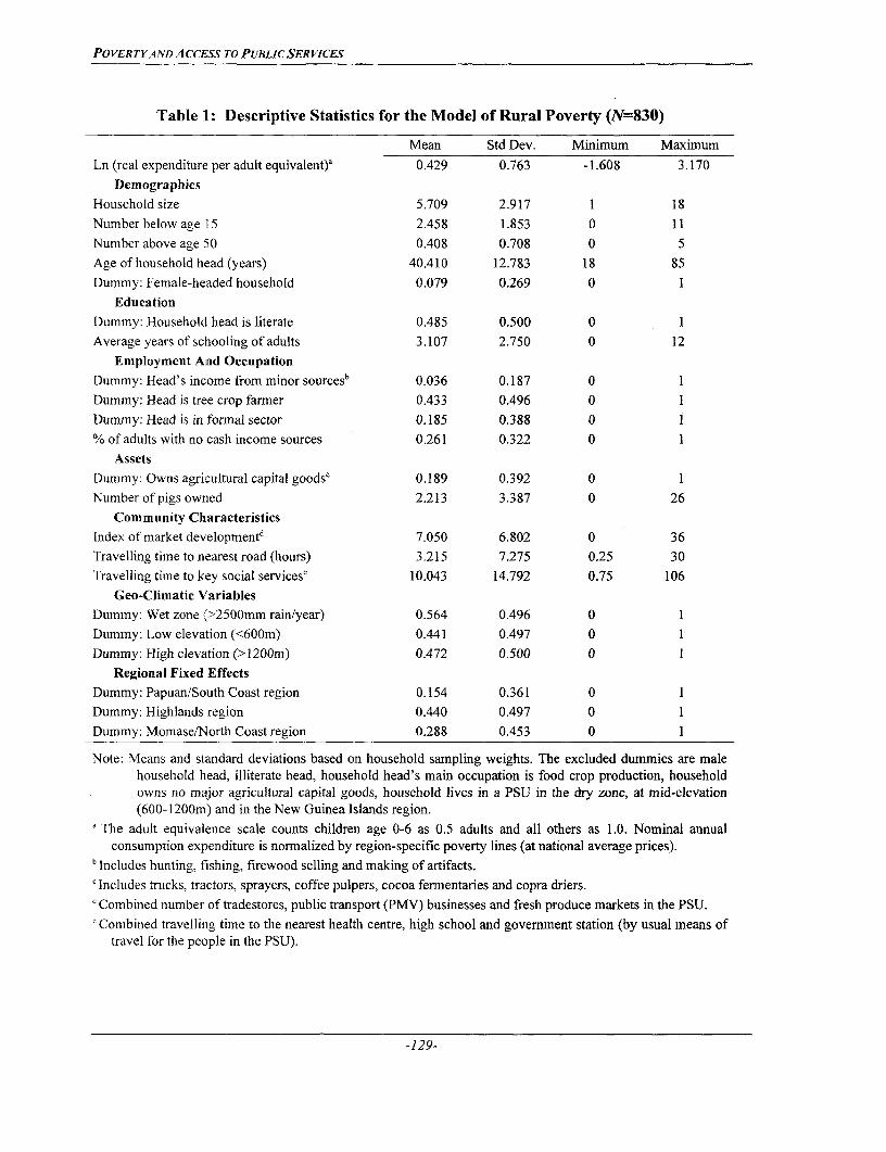
POVERTYAND ACCESS TO PUBLIC SER VICES
Table 1: Descriptive Statistics for the Model of Rural Poverty (N=830)
Mean Std Dev. Minimum Maximum
Ln (real expenditure per adult equivalent)a 0.429 0.763 -1.608 3.170Demographics
Household size 5.709 2.917 1 18Number below age 15 2.458 1.853 0 11Number above age 50 0.408 0.708 0 5Age of household head (years) 40.410 12.783 18 85Dummy: Female-headed household 0.079 0.269 0 1
EducationDummy: Household head is literate 0.485 0.500 0 IAverage years of schooling of adults 3.107 2.750 0 12
Employment And OccupationDummy: Head's income from minor sourcesb 0.036 0.187 0 1Dummy: Head is tree crop farmer 0.433 0.496 0 1Dummy: Head is in formal sector 0.185 0.388 0 1% of adults with no cash income sources 0.261 0.322 0 1
AssetsDummy: Owns agricultural capital goods' 0.189 0.392 0 1Number of pigs owned 2.213 3.387 0 26
Community CharacteristicsIndex of market developmentd 7.050 6.802 0 36Travelling time to nearest road (hours) 3.215 7.275 0.25 30Travelling time to key social servicese 10.043 14.792 0.75 106
Geo-Climatic VariablesDummy: Wet zone (>2500mm rain/year) 0.564 0.496 0 1Dummy: Low elevation (<600m) 0.441 0.497 0 1Dummy: High elevation (>1200m) 0.472 0.500 0 1
Regional Fixed EffectsDummy: Papuan/South Coast region 0.154 0.361 0 1Dummy: Highlands region 0.440 0.497 0 1Dummy: Momase/North Coast region 0.288 0.453 0 1
Note: Means and standard deviations based on household sampling weights. The excluded dummies are malehousehold head, illiterate head, household head's main occupation is food crop production, householdowns no major agricultural capital goods, household lives in a PSU in the dry zone, at mid-elevation(600-1200m) and in the New Guinea Islands region.
a The adult equivalence scale counts children age 0-6 as 0.5 adults and all others as 1.0. Nominal annualconsumption expenditure is normalized by region-specific poverty lines (at national average prices).
'Includes hunting, fishing, firewood selling and making of artifacts.'Includes trucks, tractors, sprayers, coffee pulpers, cocoa fermentaries and copra driers.' Combined number of tradestores, public transport (PMV) businesses and fresh produce markets in the PSU.'Combined travelling time to the nearest health centre, high school and government station (by usual means of
travel for the people in the PSU).
-129-

POVERTYAND ACCESS TO PUBLIC SER VICES
Table 2: Descriptive Statistics for the Model of Urban Poverty (N=314)
Mean Std Dev. Minimum MaximumIn (real expenditure per adult equivalent)a 1.365 0.909 -1.130 3.800
DemographicsHousehold size 6.552 3.466 1 23Number below age 15 2.675 1.771 0 10Number above age 50 0.369 0.678 0 3Age of household head (years) 38.838 12.419 16 72Dummy: Female-headed household 0.087 0.282 0 1
EducationDummy: Household head is literate 0.960 0.197 0 1Average years of schooling of adults 7.702 3.463 0 18
Employment and OccupationDummy: Head's income from minor 0.080 0.271 0 1sourcesb
Dummy: Head is tree crop farmer 0.086 0.281 0 1Dummy: Head is in formal sector 0.757 0.430 0 1% of adults with no cash income sources 0.298 0.270 0 1
Assets
Dummy: Owns agricultural capital goodsc 0.065 0.247 0 1
Number of pigs owned 0.381 1.436 0 8
Community CharacteristicsTravelling time to key social servicesd 1.011 0.388 0.75 2
Regional Fixed EffectsDummy: National Capital District (NCD) 0.349 0.477 0 1Note: Means and standard deviations based on household sampling weights. The excluded dummies are male
household head, illiterate head, household head's main occupation is food crop production, householdowns no major agricultural capital goods, household lives in an urban area outside of the NCD.
a The adult equivalence scale counts children age 0-6 as 0.5 adults and all others as 1.0. Nominal annualconsumption expenditure is normalized by region-specific poverty lines (at national average prices).
bIncludes hunting, fishing, firewood selling and making of artifacts.'Includes trucks, tractors, sprayers, coffee pulpers, cocoa fermentaries and copra driers.d Combined travelling time to the nearest health centre, high school and government station (by usual means of
travel for the people in the PSU).
III. RESULTS AND INTERPRETATION
13. Table 3 and 4 contains results of the basic regression models. When community,environmental and fixed effects were excluded from the model, and urban and rural samplespooled, an F-test suggested that the coefficients on household characteristics were not the sameacross urban and rural sectors (F(1690)=10.30, p<0.000), supporting the decision to estimate themodels separately. Other observations that can be made from the results are:
-130-
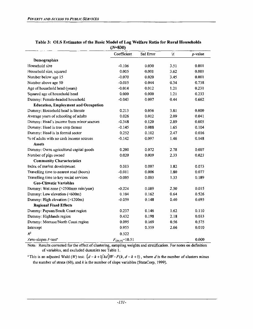
POVERTYAND ACCESS TO PUBLiC SERVICES
Table 3: OLS Estimates of the Basic Model of Log Welfare Ratio for Rural Households(N=830)
Coefficient Std Error iti p-value
DemographicsHousehold size -0.106 0.030 3.51 0.001Household size, squared 0.005 0.001 3.62 0.001Number below age 15 -0.070 0.020 3.45 0.001Number above age 50 -0.015 0.044 0.34 0.738Age of household head (years) -0.014 0.012 1.21 0.231Squared age of household head 0.000 0.000 1.21 0.233Dummy: Female-headed household -0.043 0.097 0.44 0.662
Education, Employment and OccupationDummy: Household head is literate 0.213 0.056 3.81 0.000Average years of schooling of adults 0.026 0.012 2.09 0.041Dummy: Head's income from minor sources -0.348 0.120 2.89 0.005Dummy: Head is tree crop farmer -0.145 0.088 1.65 0.104Dummy: Head is in formal sector 0.252 0.102 2.47 0.016% of adults with no cash income sources -0.142 0.097 1.46 0.148
AssetsDummy: Owns agricultural capital goods 0.200 0.072 2.78 0.007Number of pigs owned 0.020 0.009 2.33 0.023
Community CharacteristicsIndex of market development 0.013 0.007 1.82 0.073Travelling time to nearest road (hours) -0.011 0.006 1.80 0.077Travelling time to key social services -0.005 0.003 1.33 0.189
Geo-Climatic VariablesDummy: Wet zone (>2500mm rain/year) -0.224 0.089 2.50 0.015Dummy: Low elevation (<600m) 0.104 0.162 0.64 0.526Dummy: High elevation (>1200m) -0.059 0.148 0.40 0.693
Regional Fixed EffectsDummy: Papuan/South Coast region 0.237 0.146 1.62 0.110Dummy: Highlands region 0.432 0.198 2.18 0.033Dummy: Momase/North Coast region 0.095 0.169 0.56 0.575Intercept 0.955 0.359 2.66 0.010
R2 0.322
Zero-slopes F-testa F( 24. 3 n=10.51 0.000
Note: Results corrected for the effect of clustering, sampling weights and stratification. For notes on definitionof variables, and excluded dummies see Table 1.
aThis is an adJusted Wald (W)test: (d -k+I/kd)W-F(k,d -k+1), where d is thenumberofclustersminusthe number of strata (60), and k is the number of slope variables (StataCorp, 1999).
-131-
POVERTYANDACCESS TO PUBLIC SERVICES
* There are a number of significant demographic effects in both sectors. Chief among them ishousehold size: the larger the household the lower its welfare ratio, especially in the urbansector.
* There are significant gains from both extra years of schooling and literacy of the householdhead in both rural and urban areas, although the impact of education and literacy appearshigher in urban areas.
* The are significant differences in consumption level associated with occupations of thehousehold head, with involvement in the formal sector bringing the highest gains across bothsectors.
* The proportion of adults in the household without access to cash incomes in the previous yeardoes not emerge as a significant deterninant of consumption.
* Ownership of agricultural capital goods raises household consumption in both urban andrural sectors, while the number of pigs positively affects consumption in rural areas but notthe urban areas.
* Community characteristics appear to be relevant in both sectors, with consumption in therural sector rising with market development and as roads become more accessible, whileaccess to social services is an important predictor of consumption in urban areas.32
* High rainfall, but not elevation, emerges as a negative influence on consumption in ruralareas while regional fixed effects are relevant in both areas.
14. Datt and Jolliffe (1999) suggest that the marginal effects of household and communitycharacteristics on consumption are not constant across households, so introduce interactioneffects into their model to control for this. Although every variable can potentially be interactedwith every other variable, multicollinearity is likely to result, with fragile coefficient estimatesleading to potentially unreliable poverty simulations. Therefore, Datt and Jolliffe restrictattention to just a few interactions, mainly between schooling and other variables. Table 5contains results of testing for interaction effects between schooling and some other variables ineach model. The presence of interaction effects is not supported in the rural sector (p<0.43)although the coefficient on female headship is suggestive of lower returns to education forfemale-headed households.33 In the urban sector there does appear to be an interaction between
32 Travelling time to roads was not able to be used for the urban model because all PSUs had roads within theminimum specified time (0-30 minutes) and the index of market development wasn't calculated for urbanareas because the link between access to a facility and having it physically located in the PSU does not applyin urban areas - people can easily access facilities in neighbouring PSUs.
33 Even when the other four interaction effects are dropped, the interaction of school years and female headshipremains statistically insignificant (p<O. 18).
-132-

POVERTYAND ACCESS TO PUBLICSERVICES
Table 4: OLS Estimates of the Basic Model of Log Welfare Ratio for Urban Households(N=314)
Coefficient Std Error lti p-value
DemographicsHousehold size -0.205 0.043 4.80 0.000Household size, squared 0.007 0.002 4.13 0.000Number below age 15 -0.031 0.033 0.92 0.365Number above age 50 -0.129 0.071 1.82 0.076Age of household head (years) -0.015 0.021 0.72 0.473Squared age of household head 0.000 0.000 0.91 0.367Dummy: Female-headed household 0.022 0.131 0.17 0.870
Education, Employment And OccupationDummy: Household head is literate 0.346 0.216 1.60 0.117Average years of schooling of adults 0.093 0.027 3.44 0.001Dummy: Head's income from minor sources 0.321 0.218 1.47 0.148Dummy: Head is tree crop farner -0.192 0.245 0.78 0.438Dummy: Head is in formal sector 0.258 0.073 3.54 0.001% of adults with no cash income sources -0.033 0.261 0.13 0.901
AssetsDummy: Owns agricultural capital goods 0.432 0.180 2.40 0.020Number of pigs owned -0.005 0.028 0.18 0.856
Community Characteristics
Travelling time to key social services -0.804 0.234 3.43 0.001
Regional Fixed EffectsDummy: National Capital District -0.808 0.160 5.05 0.000Intercept 2.486 0.305 8.16 0.000R2 0.657
Zero-slopes F-testa F(1 7,29)=249.4 0.000Note: Results corrected for the effect of clustering, sampling weights and stratification. For notes on definition
of variables, and excluded dummies see Table AVI. 1.
a This is an adjusted Wald (W) test: (d - k + I/kd) W-F(k, d - k + 1), where d is the number of clusters minusthe number of strata (45), and k is the number of slope variables (StataCorp, 1999).
-133-

POVERTYAND ACCESS TO PUBLICSERVICES
average school years and the proportion of the adults with no involvement in cash earningactivities, so an augmented model which includes this variable is estimated for the urban sector(Table 6) and used for the poverty simulations. This augmented model suggests that the negativeeffect of unemployment on consumption in urban areas is worst for households with a low levelof schooling.
15. Table 7 reports the results of various poverty simulations done with the models in Tables4 and 6. The beneficial effect of increasing literacy, schooling and access to social services androads is readily apparent from these simulations. The incidence of poverty would fall by 16percent if all household heads could be made literate, with the greatest gains in the rural sector.Although the incidence of poverty would fall by only 4.5 percent, following a one year rise inaverage school years per adult, a much larger effect (-20.4 percent) is observed in the urbansector. The headcount index would fall by 6.6 percent if the travelling time to key social servicescould be cut by 50 percent, with the greatest proportionate gain in the urban sector. Reducing thetravelling time to the nearest road would also be an effective anti-poverty strategy in the ruralsector, with the greatest gains from an approach targeted on the most remote households ratherthan on making across-the-board cuts in travelling time to roads.
Table .5: Interaction Effects Between Average Years of Schooling of Adults in the Householdand Other Household and Community Characteristics
Variable interacted with: Rural UrbanDummy: Female headed household -6.7496 -1.2362
(1.68) (0.35)% of adults with no cash income source 2.9893 14.0930
(0.85) (1.98)Dummy: Owns agricultural capital goods 0.4818 ...
(0.23)Index of market development -0.1521 ...
(1.06)Travelling time to nearest road -0.0050 ...
(1.19)
F-test for joint significance F(5 ,56)=1.00 F(2,44)=3.24Note: All coefficients multiplied by 100. Numbers in () are t-statistics, corrected for sample design effects.
-134-

POVERTYAND ACCESS TO PUBLICSERVICES
Table 6: OLS Estimates of the Augmented Model of Log Welfare Ratio for Urban Households
Coefficient Std Error |t| p-value
DemographicsHousehold size -0.237 0.049 4.81 0.000Household size, squared 0.009 0.002 3.94 0.000Number below age 15 -0.034 0.035 0.98 0.334Number above age 50 -0.096 0.067 1.45 0.155Age of household head (years) -0.010 0.022 0.46 0.647Squared age of household head 0.000 0.000 0.55 0.589Dummy: Female-headed household 0.028 0.116 0.24 0.809
Education, Employment and OccupationDummy: Household head is literate 0.322 0.185 1.74 0.088Average years of schooling of adults 0.056 0.039 1.45 0.155Dummy: Head's income from minor sources 0.246 0.239 1.03 0.311Dummy: Head is tree crop farmer -0.356 0.300 1.19 0.242Dummy: Head is in formal sector 0.190 0.083 2.28 0.027% of adults with no cash income sources -1.167 0.729 1.60 0.116(Average school years) x (% no cash 0.143 0.068 2.09 0.042income)
AssetsDummy: Owns agricultural capital goods 0.474 0.169 2.81 0.007Number of pigs owned -0.015 0.035 0.43 0.669
Community CharacteristicsTravelling time to key social services -0.827 0.239 3.46 0.001
Regional Fixed EffectsDummy: National Capital District -0.790 0.156 5.07 0.000Intercept 2.939 0.409 7.19 0.000R2 0.673Zero-slopes F-testa F(1 8,28)=271.9 0.000Note: Results corrected for the effect of clustering, sampling weights and stratification. For notes on definition
of variables, and excluded dummies see Table 1.
a This is an adjusted Wald (W) test: (d - k + i/kd) W-F(k, d - k + 1), where d is the number of clustersminus the number of strata (45), and k is the number of slope variables (StataCorp, 1999).
-135-
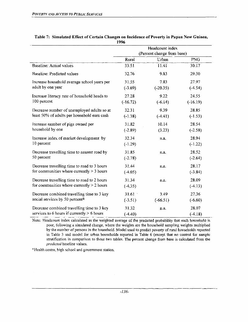
POVERTYAND ACCESS TO PUBLIC SER VICES
Table 7: Simulated Effect of Certain Changes on Incidence of Poverty in Papua New Guinea,1996
Headcount index(Percent change from base)
Rural Urban PNG
Baseline: Actual values 33.51 11.41 30.17
Baseline: Predicted values 32.76 9.83 29.30
Increase household average school years per 31.55 7.83 27.97adult by one year (-3.69) (-20.35) (-4.54)
Increase literacy rate of household heads to 27.28 9.22 24.55100 percent (-16.72) (-6.14) (-16.19)
Decrease number of unemployed adults so at 32.31 9.39 28.85least 50% of adults per household earn cash (-1.38) (-4.41) (-1.53)
Increase number of pigs owned per 31.82 10.14 28.54household by one (-2.89) (3.23) (-2.58)
Increase index of market development by 32.34 n.a. 28.9410 percent (-1.29) (-1.22)
Decrease travelling time to nearest road by 31.85 n.a. 28.5250 percent (-2.78) (-2.64)
Decrease travelling time to road to 3 hours 31.44 n.a. 28.17for communities where currently > 3 hours (-4.05) (-3.84)
Decrease travelling time to road to 2 hours 31.34 n.a. 28.09for communities where currently > 2 hours (-4.35) (-4.13)
Decrease combined travelling time to 3 key 31.61 3.49 27.36social services by 50 percenta (-3.51) (-66.51) (-6.60)
Decrease combined travelling time to 3 key 31.32 n.a. 28.07services to 6 hours if currently > 6 hours (-4.40) (-4.18)
Note: Headcount index calculated as the weighted average of the predicted probability that each household ispoor, following a simulated change, where the weights are the household sampling weights multipliedby the number of persons in the household. Model used to predict poverty of rural households reportedin Table 3 and model for urban households reported in Table 6 (except that no control for samplestratification in comparison to those two tables. The percent change from base is calculated from thepredicted baseline values.
a Health centre, high school and government station.
-136-

POVERTYAND ACCESS To PUBLICSERVICES
ANNEX VII: PRIVATE TRANSFERS AND THE SOCIAL SAFETY NET IN PAPUA NEW GUINEA3 4
I. INTRODUCTION
1. This annex uses a model developed by Ravallion and Dearden (1988) to study thedistribution of transfer receipts amongst recipient households surveyed during the 1996household survey. The objective is to see whether transfer receipts are effectively targeted at theneedy and improve income distribution.
II. THE RAVALLION AND DEARDEN MODEL
2. If tdr is the transfer made by donor d to recipient r, it is assumed that the values of tdr arechosen by the donor to maximise the function:
U (Yi, XI, ... , Yd, Xd,...,Yfl,Xf) (I)
where Yi is the income after transfers of household i and Xi is a vector of other attributes of i.The maximization is constrained by:
Yr f (tdr, Xr) (2)
nYd = Yd> tdr (3)
r=l
where Yd is the donor's (fixed) pre-transfer income and it is assumed that aYr /atdr is non-negative.' At an optimum, the donor's marginal utility from giving an extra dollar cannot exceedthe donor's marginal utility of own-income (otherwise they will give the extra dollar so theprevious state cannot have been optimal), thus:
a2u> au - and tdr Ž 0 with complementary slackness. (4)a Yd Dyl td
3.To put explicit, and tractable, functional forms on the three derivatives in equation (4),Ravallion and Dearden assume that:
(i) each donor's utility function is of constant elasticity of substitution (CES) in thevector of recipients' incomes, and the elasticity of substitution is constant acrossdonors,
(ii) donor's utility functions are separable between own-income and the incomes ofothers,
(iii) donor's marginal utility of own-income is iso-elastic in own-income, with thesame elasticity across donors
(iv) recipient's incomes are iso-elastic in their total transfer receipts, with a constantelasticity across recipients.
34 Based on Gibson, J. (1999c), "Is there a Malenesian Moral Economy? Private Transfers and the Social Safety Netin Papua New Guinea", Mimeo, Prepared for Poverty Assessment.
-137-
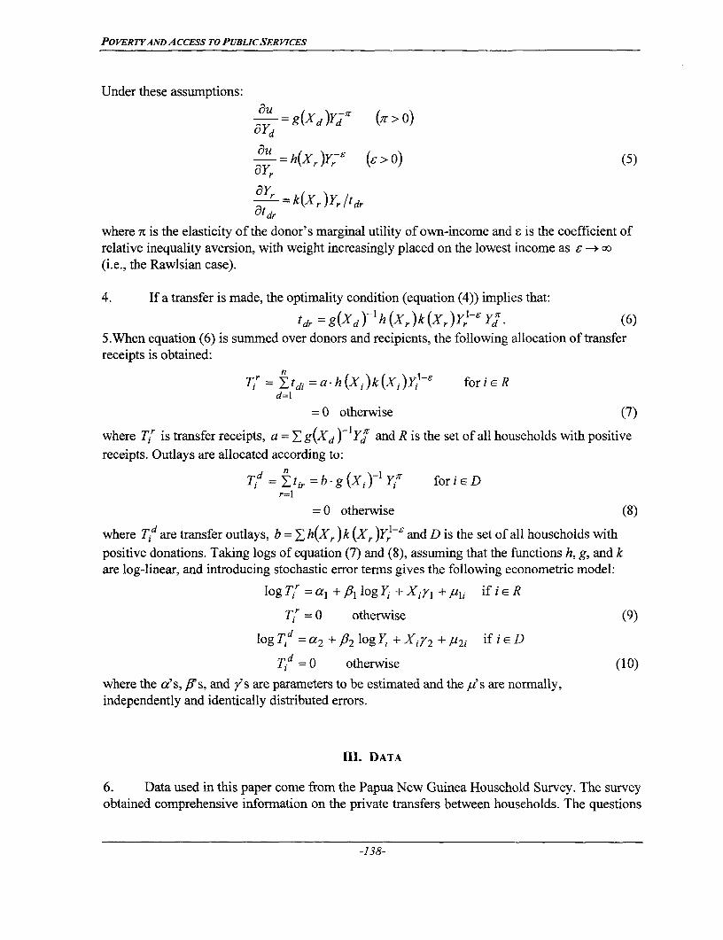
POVERTYAND ACCESS TO PUBLIC SER VICES
Under these assumptions:
=g(Xd )Yd (IT > O)Yd
au hI(Xr )Y (>o 0) (5)
at = k(Xr )Y, ltdr
where 7r is the elasticity of the donor's marginal utility of own-income and E is the coefficient ofrelative inequality aversion, with weight increasingly placed on the lowest income as -* Co(i.e., the Rawlsian case).
4. If a transfer is made, the optimality condition (equation (4)) implies that:
tdr =g(Xd)Ih(X,)k(X,)Y,6 Yd. (6)
5.When equation (6) is summed over donors and recipients, the following allocation of transferreceipts is obtained:
nTi = ,tdi =a -h (Xi)k(Xi)Yi forieR
d=1
=0 otherwise (7)
where Tir is transfer receipts, a = E g(Xd ) 1 Yd and R is the set of all households with positivereceipts. Outlays are allocated according to:
Tid = tir =b-g(Xj)lYj foriEDr=1
= 0 otherwise (8)
where Ti.d are transfer outlays, b = E h(Xr ) k (Xr )Yk'-8 and D is the set of all households withpositive donations. Taking logs of equation (7) and (8), assuming that the fumctions h, g, and kare log-linear, and introducing stochastic error terms gives the following econometric model:
logT/ = 1 +11og17 + Xi7y +±u1 i if ieR
Tir =0 otherwise (9)dlog T = a2 +,62 log Yi + Xiy 2 + l2i if i E DdTid = 0 otherwise (10)
where the a's, ifs, and i s are parameters to be estimated and the u's are normally,independently and identically distributed errors.
III. DATA
6. Data used in this paper come from the Papua New Guinea Household Survey. The surveyobtained comprehensive information on the private transfers between households. The questions
-138-

POVERTYAND ACCESS To PUBLiC SER VICES
about the production and purchase of each food item during the consumption recall period alsoasked about inward and outward transfers of those food items, with a similar format used for thenon-food frequent expenses. The questions about each category of infrequent expenses alsoasked about the value of in-kind gifts given and received of these items during the previous 12months. Details were also obtained on each inward and outward monetary transfer exceedingK50 in the previous 12 months, with additional questions asked about the destination (origin) ofthis transfer, the relationship of the household head to the recipient (donor), and whether anyspecific purpose was stipulated for the transfer.
IV. MODEL SPECIFICATION
7. Table 2 describes the explanatory variables used in the models of transfers. Wherepossible, the variables used by Ravallion and Dearden (1988) are chosen. One exception was thatthe survey did not obtain inforrnation on deaths within the household during the previous year.The replacement variable used is whether the household is headed by a female, which mayreflect widowhood which is likely to motivate transfer receipts in the same way that a recentdeath does. Also, because the Ravallion and Dearden study was for just one province in centralJava (Yogyakarta), while the current study is for the whole of PNG, regional dummy variableshave been added to the model. These dummies should capture regional price differences and alsoproxy for other excluded locational effects.
Table 2: Explanatory variables used in the models of transfersMean (Std. Dev)
Variable Rural Urban Description
Expenditures 3736 11299 Annual value of household total expenditure (including(3812) (8785) imputed value of stock changes, own-production, and
gifts received) and excluding the value of gifts given.
Household size 5.709 6.552 Total number of residents usually present in the(2.92) (3.47) household at the time of the survey.
111-health 0.727 0.592 Average number of times treated at health facilities per(1.33) (1.70) person in the month prior to the survey.
Births 0.193 0.225 Dummy variable =1 if anyone in the household was(0.39) (0.42) born in the 12 months prior to the survey.
Head's age 40.4 38.8 Years of age of the household head.
(12.8) (12.4)
Female head 0.079 0.087 Dummy variable =1 if the household head is female.
(0.27) (0.28)
Unemployment 0.150 0.057 Dummy variable =1 if household head had no source of(0.36) (0.23) cash income in the 12 months prior to the survey.
-139-
POVERTYAND ACCESS To PUBLICcSER VICES
The income term in Ravallion and Dearden's model is a metric of each household's welfare aftertransfers, and in this regard it differs from other studies which focus on pre-transfer income. Theempirical income variable used by Ravallion and Dearden was the predicted value of (log) totalhousehold consumption of all goods and services, excluding expenditure on gifts. Predictedvalues were needed because household consumption is a function of transfer receipts, and thissimultaneity violates the independence of the regressor from the model error term. Theinstruments used for log consumption by Ravallion and Dearden were: labor earnings, incomefrom enterprises, rents received, years of schooling, dwelling characteristics, occupationaldummy variables, and the variables in the Xvector in equations x and y.
8. It was not possible to use all of these instruments in the current study because the PNGsurvey did not calculate cash incomes. However, data on certain assets were available (the valueof household durables, ownership of agricultural capital goods like coffee pulpers, copra driersand trucks, and the number of pigs owned), and these should be correlated with cash incomes.Additionally, a cluster-level variable measuring the travelling time to the nearest transportfacility (road, airstrip or port) was included for the rural sector, because inaccessibility is a majorconstraint on cash incomes in PNG. The other instruments included the head's years ofschooling, characteristics of the dwelling (floor area and roof type) and a vector of threeoccupational dummy variables indicating the household head's main source of cash income(agriculture, running a business, wages). These instruments raised the R2 in the first stageequation predicting log expenditures from 0.33 to 0.47 in the rural sector and from 0.20 to 0.60in the urban sector and F-tests suggested that the instruments were highly significant predictorsof log expenditures (see Appendix Table 1).
-140-

POVERTYAND ACCESS TO PUBLICSERVICES
V. RESULTS AND INTERPRETATION
9. The coefficient A1 in equation (9) can be considered the elasticity of transfer receipts withrespect to income. Three scenarios for the value of A pose different interpretations on thepreferences that the donor has over the resulting income distribution. If A = 1, transfers rise orfall proportionate to recipient households change in income, and therefore transfers are a constantshare of recipient household income. A donor giving to two households, one rich and one poor,makes transfers proportionate to each households income so if before transfers the rich householdwas twice as rich as the poor household, it will also be twice as rich after the transfer. Thedistribution of income is not altered, implying no aversion to inequality on the part of peopledonating transfers. If ,Ai < 1, transfers do not rise as fast as income rises, so transfers wouldcontribute a bigger share to the post-transfer consumption of a poor household than of a richhousehold, and in this way transfers reduce disparities in income and makes the distribution moreequal. Therefore, an elasticity of transfer receipts with respect to income less than one impliesaversion to inequality on the part of the people donating transfers. Conversely, if A, > 1,transfers increase disparities in income and makes the distribution more unequal than it wasbefore, indicating donors' preference for inequality.
10. Table 3 reports the results for gross and net receipts of transfers. Recall that grosstransfers are relevant if it is assumed that donors hold myopic expectations. Specifically, myopicexpectations hold if donors decide how much to donate without taking account of any reversetransfers that the recipient may make to them in future and also ignoring any passing on of theirdonation by the recipient to someone else. If donors hold rational expectations of recipients'behaviour, taking into account return transfers and the passing on of transfers to others, then it isthe net transfer that is relevant. Although the information requirements for rational expectationsare high, it is plausible that donors who are engaged in long term relationships with recipients,and are often kinsfolk, can correct anticipate recipients behaviour on average.
11. In the Table 3 results, the hypothesis that ,A,=1 (no inequality aversion) is rejected at thep<0.04 level in favour of the alternative hypothesis that ,B,>1 (i.e., transfers are inequalityincreasing) when using gross receipts. The null of no inequality aversion is not rejected for therural sector in the model using net receipts (p<O.6 1). In the urban sector, the null of no inequalityaversion is not rejected for the model using gross receipts (p<0.17) but in the model of netreceipts it is rejected at the p<0.09 level in favour of the alternative hypothesis of inequalityaversion.
12. The other factor relevant to transfer receipts in both rural and urban sectors is femaleheadship of the household, which may reflect remittances from absent husbands but could alsoreflect targeting of widows. Transfer receipts for rural households also rise if there was a birth inthe last year, and if the household head has no source of cash income during the past year (for netreceipts only).
-141 -
POVERTYAND ACCESS TO PUBLIC SER VICES
13. Table 4 reports the results of repeating the econometric analysis, but this timeconcentrating on the transfers made on a day-to-day basis - that is, transfers of food and othersmall expenditure items (e.g., betelnut, cigarettes, PMV fares). In the gross receipts equation, thecoefficient on A3, is smaller for both sectors, indicating slightly more inequality aversion by thedonors of day-to-day transfers than was apparent when considering the total transfers. However,the pattern of transfers having a more equalising role in urban than rural sectors is repeated.Another notable result from Table 4 is that female headship remains a relevant factor in thereceipt of small daily transfers. This counts against the idea that the significance of femaleheadship in Table 3 is just due to remittances from long-distance husbands, because it is unlikelythat such husbands could send food and other small items on a day-to-day basis.
14. Table 5 reports the results of repeating the analysis on the longer term transfers, whichwere measured with an annual reference period. These include transfers of cash and of goods andservices in-kind (e.g., buying household equipment and giving it to a relative, paying the schoolfees of a friend's child). The results for gross receipts are clearest, and show that in comparisonto day-to-day transfers and also total transfers, it is the transfers made on an annual basis whichshow the least aversion to inequality (especially in the rural sector); This may be because theseindividually larger transfers take place in ceremonial events (e.g. contributing to bride-price)where people are obligated to participate, even if it means poorer households donating to richerhouseholds.
-142-

POVERTYAND ACCESS TO PUBLIC SER VICES
Table 3: Two-stage Tobit estimates of the receipts equationGross Receipts Net Receipts
Rur'al Urban Rural Urban3 Iti 3 I' 3 lti (
In expenditures' 1.544 6.27 0.483 1.31 1.265 2.46 -1.204 0.964In household size -0.498 2.44 0.048 0.13 -0.464 1.01 0.292 0.421Ill-health 0.050 1.02 0.083 1.38 0.089 0.65 0.244 1.690Births (=1) 0.726 4.11 0.068 0.26 2.016 3.56 0.658 0.636Head's age -0.047 1.34 -0.104 0.95 0.129 1.07 -0.104 0.490[Head's age]2 0.001 1.35 0.001 1.08 -0.001 0.92 0.002 0.633Female head (=1) 0.550 2.05 0.702 2.03 1.425 1.91 1.921 1.520Unemployment (=1) 0.299 0.95 0.219 0.35 1.196 2.60 0.195 0.089Papuan region (=1) -0.654 1.50 .. .. -3.137 3.80
Highland region (=1) -0.320 1.00 .. .. -1.411 2.16
Momase region (=1) -0.662 1.74 .. .. -1.516 2.12
NCD region (=1) .. .. 0.376 0.83 .. .. 0.790 0.63
Constant -5.024 2.68 2.596 0.71 -10.53 2.09 11.778 1.27Zero-slopes F-test 10.45 7.05 6.42 4.24
Prob(Ti> 0X) 0.926 0.890 0.507 0.487
Note: Reported absolute t-values are corrected for clustering, sampling weights and sample stratification. F-
test is an adjusted Wald (W) test: ((d - k + l)/kd) W-F(k, d - k + 1), where d is the number ofclusters minus the number of strata (60 for rural and 45 for urban), and k is the number of slopevariables. The excluded region in the rural sector is the New Guinea Islands, and in the urban sectorit is all urban areas outside of the National Capital District (NCD).
'Predicted value used for In expenditures, with predictions from the model in Appendix Table 1.
-143-

POVERTYANDA CCESS TO PUBLICSERVICES
Table 4: Two-stage Tobit estimates of the receipts equation - day-to-day transfers
Gross Receipts Net ReceiptsRural Urban Rural Urban
13 itt 1 itt D Itl D ittIn expendituresa 1.259 4.08 0.385 0.80 0.819 1.33 0.335 0.34In household size -0.448 1.84 -0.165 0.40 -0.210 0.40 0.098 0.16111-health 0.091 1.82 0.107 1.30 0.124 0.98 0.132 1.05Births (=1) 0.545 2.23 -0.506 0.92 1.816 3.37 -0.531 0.62Head's age -0.049 1.20 0.017 0.15 0.145 1.61 -0.095 0.50[Head's age]2 0.000 0.97 0.000 0.22 -0.001 1.23 0.001 0.66Female head (=1) 0.695 2.20 0.742 2.02 1.167 1.99 2.864 3.04Unemployment (=1) -0.040 0.15 0.477 0.76 0.123 0.23 -2.071 1.34Papuan region (=1) -0.683 1.70 -3.115 3.95Highland region (=1) -0.793 2.64 -1.342 1.79Momase region (=1) -1.132 2.54 -2.129 2.56NCD region (=1) 0.202 0.32 1.254 1.48Constant -2.985 1.29 0.953 0.25 -7.759 1.57 -0.714 0.10
Zero-slopes F-test 5.45 2.94 6.28 4.79
Prob (T > 01X) 0.865 0.815 0.511 0.551
Note: Reported absolute t-values are corrected for clustering, sampling weights and sample stratification.
F-test is an adjusted Wald (W) test: ((d - k + I)/kd) W-F(k, d - k + 1), where d is the number of clustersminus the number of strata (60 for rural and 45 for urban), and k is the number of slope variables.The excluded region in the rural sector is the New Guinea Islands, and in the urban sector it is all urbanareas outside of the National Capital District (NCD).a'Predicted value used for In expenditures, with predictions from the model in Appendix Table 1.
-144-
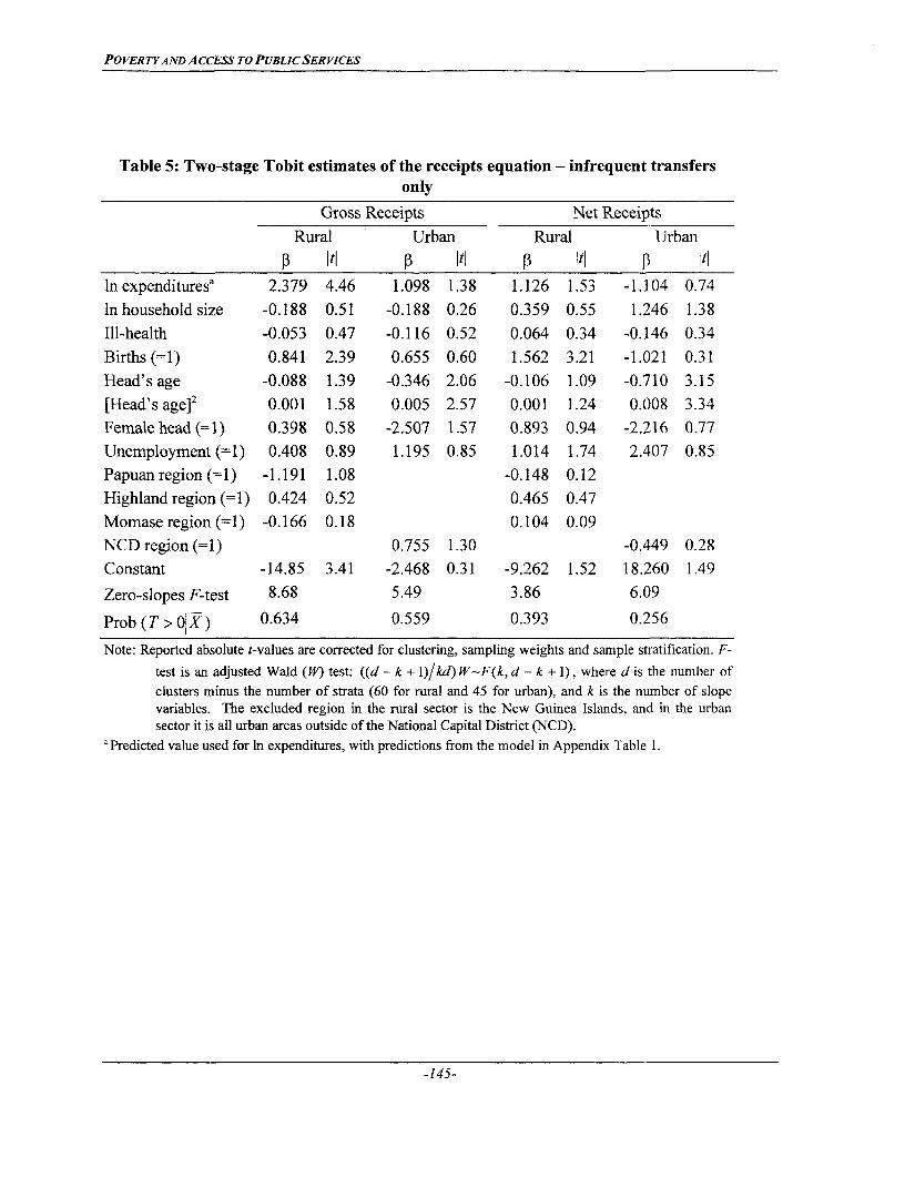
POVERTYANDACCESS TO PUBLICSERVICES
Table 5: Two-stage Tobit estimates of the receipts equation - infrequent transfersonly
Gross Receipts Net ReceiptsRural Urban Rural Urban
3 iti 1 ItI D It Iti
In expendituresa 2.379 4.46 1.098 1.38 1.126 1.53 -1.104 0.74Inhousehold size -0.188 0.51 -0.188 0.26 0.359 0.55 1.246 1.38Ill-health -0.053 0.47 -0.116 0.52 0.064 0.34 -0.146 0.34Births (=1) 0.841 2.39 0.655 0.60 1.562 3.21 -1.021 0.31Head's age -0.088 1.39 -0.346 2.06 -0.106 1.09 -0.710 3.15[Head's age]2 0.001 1.58 0.005 2.57 0.001 1.24 0.008 3.34Female head (=1) 0.398 0.58 -2.507 1.57 0.893 0.94 -2.216 0.77Unemployment (=1) 0.408 0.89 1.195 0.85 1.014 1.74 2.407 0.85Papuan region (=1) -1.191 1.08 -0.148 0.12Highland region (=1) 0.424 0.52 0.465 0.47Momase region (=1) -0.166 0.18 0.104 0.09NCD region (=1) 0.755 1.30 -0.449 0.28Constant -14.85 3.41 -2.468 0.31 -9.262 1.52 18.260 1.49
Zero-slopes F-test 8.68 5.49 3.86 6.09
Prob (T > ol0x) 0.634 0.559 0.393 0.256
Note: Reported absolute t-values are corrected for clustering, sampling weights and sample stratification. F-
test is an adjusted Wald (W) test: ((d - k + I)/kd) W-F(k, d - k + 1), where d is the number ofclusters minus the number of strata (60 for rural and 45 for urban), and k is the number of slopevariables. The excluded region in the rural sector is the New Guinea Islands, and in the urbansector it is all urban areas outside of the National Capital District (NCD).
a Predicted value used for In expenditures, with predictions from the model in Appendix Table 1.
-145-

POVERTYAND ACCESS TO PUBLIC SERVICES
Table 6: Two-stage Tobit estimates of the outlays equation
Gross Outlays Net OutlaysRural Urban Rural Urban
In expendituresa 1.630 6.97 0.779 2.16 0.284 0.48 1.972 1.56ln household size -0.901 4.51 -0.339 1.00 -0.190 0.38 -0.346 0.54Ill-health -0.071 1.28 -0.255 2.83 -0.126 0.76 -0.224 0.81Births (=1) 0.099 0.50 -0.066 0.13 -2.040 2.80 -0.700 0.64Head's age -0.014 0.37 -0.135 1.37 -0.167 1.41 0.084 0.34[Head's age]2 0.000 0.20 0.001 1.48 0.002 1.31 -0.001 0.37Female head (=1) -0.495 1.18 -1.192 1.89 -1.185 1.18 -2.776 1.79Unemployment (=1) 0.038 0.11 0.427 0.67 -1.574 2.94 0.641 0.26Papuan region (=1) 0.368 1.21 3.596 3.60Highland region (=1) 0.122 0.53 2.108 2.24Momase region (=1) 0.022 0.07 1.767 1.76NCD region (=1) 0.212 0.70 -0.618 0.55Constant -5.847 3.16 2.100 0.48 0.910 0.17 -17.23 1.60Zero-slopes F-test 8.34 6.58 6.12 4.15
Prob(T>OIX) 0.918 0.916 0.473 0.496
Note: Reported absolute t-values are corrected for clustering, sampling weights and sample stratification.
F-test is an adjusted Wald (W) test: ((d - k + )/Ikd) W-F(k, d - k + 1), where d is the number of clustersminus the number of strata (60 for rural and 45 for urban), and k is the number of slope variables.The excluded region in the rural sector is the New Guinea Islands, and in the urban sector it is all urbanareas outside of the National Capital District (NCD).a Predicted value used for In expenditures, with predictions from the model in Appendix Table 1.
-146-

POVERTYAND A CCESS TO PUBLIC SERVICES
Appendix Table 1: First stage regressions predicting In (household expenditures)
Rural Urban
Itl iti
Head's years of school 0.031 4.03 0.038 4.67Floor area of dwelling 0.003 2.23 0.006 7.21Iron roof on dwelling 0.457 5.45 0.382 1.43
Agricultural capital goods owned 0.155 2.01 0.286 1.86Number of pigs owned 0.022 2.44 -0.040 1.21Value of household durables 0.000 6.65 0.000 9.56
Walking time to nearest road etc' -0.001 1.22 ... ...Household head's main cash incomefrom:
Agriculture 0.200 1.60 -0.504 3.86Running a business 0.274 1.71 -0.063 0.21Wage employment 0.425 3.07 -0.032 0.16
In household size 0.498 8.60 0.098 1.26Ill-health 0.043 2.62 0.011 0.88Births (=1) -0.087 0.81 0.263 1.52Head's age -0.005 0.39 -0.001 0.04[Head's age]' 0.000 0.53 0.000 0.10Female head -0.003 0.03 0.014 0.14Unemployed head (nil income) 0.085 0.55 -0.279 1.29
Regional intercepts
Papuan/South Coast 0.376 3.13Highlands 0.449 3.38Momase/North Coast -0.183 1.20National Capital District * - 0.212 1.83
Constant 6.308 17.42 7.728 13.76
R 2 0.47 0.60
Zero-slopes F-test 25.47 185.99
F-test on additional instruments 20.47 77.50
N=830 N=314
Note: Reported absolute t-values are corrected for clustering, sampling weights and sample stratification. F-
test is an adjusted Wald (W) test: ((d - k + I)/kd) W-F(k, d - k + 1), where d is the number ofclusters minus the number of strata (60 for rural and 45 for urban), and k is the number of slopevariables.
a Airstrips and berthing points for water transport vessels are used if they are closer than roads. All urbanareas have transport facilities accessible within the minimum category for walking time (0-30 minutes).
This does not rule out disincentive effects of transfers, which occur if the derivative is less than one, nor positiveproductivity effects of transfers, which occur if the derivative exceeds one.
-147-