order and disorder lines in systems with competing interactions: ii. the irf model

Journal of Statistical Physics, VoL 29, No. 2, 1982

Order and Disorder Lines in Systems with Competing Interactions: II. The IRF Model

P. Rujdn 1,2

Received March 15, 1982

Systems with competing interactions can be often exactly solved on a restricted subspace of the parameter space, called an order or disorder trajectory. A simple method introduced within the transfer matrix formalism allows for the calculation of the free energy and spin-spin correlation functions along the order and disorder lines of the Ising model with all possible interactions around a face of the square lattice (IRF model). The general eight-vertex model is thoroughly examined and shows full analogy with the quantum spin chain results of the previous paper.

KEY WORDS: Eight-vertex model; interactions around a face; order and disorder lines; transfer matrix.

1. INTRODUCTION

This is the second in a series of papers devoted to the study of order (OL) and disorder (DOL) lines in different models with competing interactions. These lines (or surfaces) run through the space of interaction parameters and are characterized by a minimum of the correlation length along the competition axis. In many respects there is a strong resemblance between the properties of the spin-spin correlation functions near a disorder or order line and, respectively, near a phase boundary. For example, the spin-spin correlation functions change in character and also display non- analytic behavior when a DOL(OL) is crossed at fixed temperature/l) However, this behavior does no t reflect a phase transition. Also, this

i Northeastern University, Boston, Massachusetts 02115. z On leave from and address after September 1, 1982: Institute for Theoretical Physics, Eotv6s

University, 1088 Budapest, Puskin U. 5-7, Hungary.

247 0022-4715/82/1000-0247503.00/0 �9 1982 Plenum Publishing Corporation

248 Ruj=~n

peculiar behavior is associated to a minimum rather than to a maximum of the correlation length.

In the previous paper, (1) referred to hereafter as I, the concept of OL(DOL) was introduced for quantum spin systems at T = 0, where the method of Peschel and Emery (2) allows to extract a variety of useful information. In view of the rigorous (and approximate) relationship between quantum spin chain Hamiltonians and transfer matrices of two- dimensional models, (3) one expects order and disorder lines in these latter models as well. The main goal of this paper is to introduce a simple method for the calculation of the free energy and of correlation functions along the OL(DOL) in two-dimensional models. This method is close in spirit to the method used by Kurman, Thomas, and Muller, (4) who recently calculated the order surface of the one-dimensional X Y Z antiferromagnetic chain in an arbitrary field at T = 0.

In Section 2 the "interactions-around-a-face" (IRF) model is defined on a square lattice and its row-to-row transfer matrix is constructed. The connection to quantum formalism is made clear and it is shown how to choose an ansatz for the eigenvector ("ground state") corresponding to the largest eigenvalue ("ground state energy") of the transfer matrix. It turns out that the order surface of the IRF model is beyond the "horizon" of the Boltzmann weights. When an appropriate analytic continuation is made for the IRF model with an even interactions only (even model) one recovers the form (2.17) obtained in I. In Section 3 the diagonal-to-diagonal transfer matrix is constructed and given in terms of Pauli matrices. A properly chosen ansatz is shown to be the ground state on the disorder surface. For the even model (which is the dual of the eight-vertex model) it is shown that a duality transformation maps the order surface into the disorder surface and vice versa. Finally, in Section 4 the formalism is applied to the Ising model with ferromagnetic nearest-neighbor (n.n.) interactions and antiferromagnetic next-nearest-neighbor (n.n.n.) (diagonal) interactions.

2. ORDER AND DECOUPLING LINES FROM THE ROW-TO-ROW TRANSFER MATRIX

Consider an n • m square lattice with Ising spin varibles defined on the lattice sites. The spins interact with all possible interactions within a basic square (or face). The Boltzmann weight of such a face (Fig. 1) is given by

K . = (2.1) Following Baxter (s) we call this model an "interactions-around-a-face"

Order and Disorder Lines in Systems with Competing Interactions: II

I I

S~ S 2

249

W

S I S 2

Fig. 1. The basic face bordered by the spins sl, s2, s~, and s~. All possible interactions are allowed between these spins.

(IRF) model. The partition function of IRF models is given by

Z({K~ )) = ~]. Hw(so,sj+l[si+, , j ,s i+14+, ) (2.2) (s,y= - 1} i , j

If the partition function Z is expressed as a function of the different weights {w} instead of the interactions {K,~}, the IRF model is given in "weight representation" rather than in the "interaction representation." Supposing one has periodic boundary conditions, the partition function (2.2) can be thought as being the iterated kernel of a linear integral operator transferring the interactions from one row of spins to the next row of spins. In matrix representation the row-to-row transfer operator is defined as

TRR,,s" ---- I- '[w(j ,J + 1),.s, (2.3) J

where s = (sl,s2 . . . . . s,), s ' = ( s { , s ~ , . . . , s;,) represent the configuration space of the ith and (i + 1)th row, respectively, and

, �9 . . . . . S t S ~ "~ w ( j , j + 1)s,~,= 6s~i 6,~,,~ 6~j_~,~j_w(sj ,Sj+ 1 ] ~/-, ~/+1)

• %+>5"+2"'' %.,*; (2.4)

The partition function is expressed as

g = Tr(T~R)m-----~3,# = e ""f (2.5) - " r t ' / - - > ~

250 Rujan

where X0 is the largest eigenvalue of the transfer matrix and f is the free energy per spin

f = - F / k B Tmn (2.6)

Similarly, the correlation functions between spins lying on two next- nearest-neighbor rows is given by

<q,01AB Iq,0> (A(s)~(s')) - <~ol ~o> (2.7)

where [t)o > is the ground state corresponding to X o, and A and B are given functions of spins. In particular,

a~ = @o1%%.+R1+o> <q,01%> (2.8)

corresponding to Eq. (3.3) of I. The correlation functions between spins situated on rows R distance

apart is given by

<A = 2 f 1" No ] <+~176 (2.9)

In particular

Xq )R G~- = ( s O . s ~ + . j > ~ ( ~oo I@~ (2.10)

where X 0 is the largest eigenvalue (Xq < h0) corresponding to a nonzero @01slq~q> matrix element.

The calculation of G~ requires the knowledge of Xq, i~q) in addition to X0, I%> and cannot be calculated by our method.

Now we turn back to the study of the transfer matrix (2.3)-(2.4). In order to make clear the analogy with the quantum formalism one needs a representation-independent form. Following Baxter, (s'6) one expands the w ( j , j + 1) matrices in terms of the Pauli matrices 01= ox; o 2 = oxoz; 0 3 = 0 z and 0 4 = 1 as

4 4

[w(j,j + 1)Is,s,= E E e,J,o,:d,:2,j+, (2.11) J ~ l J ' = l

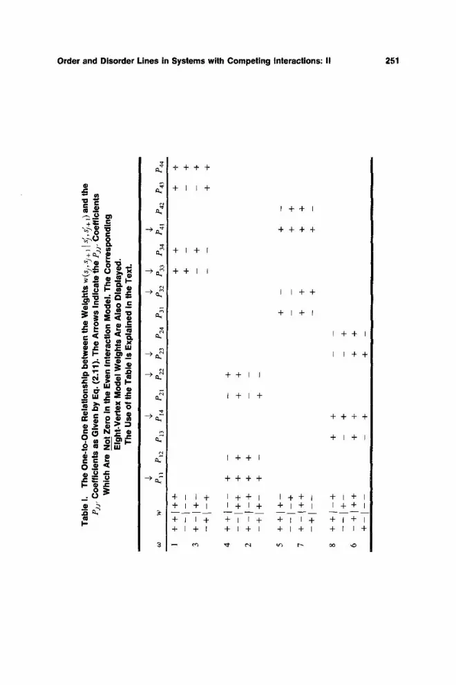
where os/~ is the (a, t ) element of the o J Pauli matrix. The one-to-one relationship between the coefficients Pss" and the Boltzmann weights w (or to in terms of the eight-vertex model) is given in Table I. A given Pss" coefficient should be calculated by adding with the corresponding sign the different weights w (a blank space means a zero table element) and by

Ta

ble

I.

Th

e O

ne

-to

-On

e R

ela

tio

nsh

ip b

etw

ee

n t

he

We

igh

ts w

(sj,

sj+ 1

I s~,

s~+ 1

) an

d t

he

P

jj,

Co

eff

icie

nts

as

Giv

en

by

Eq

. (2

.11)

. T

he

Arr

ow

s In

dic

ate

th

e P

gs, C

oe

ffic

ien

ts

Wh

ich

Are

No_

_tt Z

ero

In

the

Eve

n I

nte

racU

on

Mo

de

l, T

he

Co

rre

spo

nd

ing

E

igh

t-V

ert

ex

Mo

de

l W

eig

hts

Are

Als

o D

isp

laye

d.

Th

e U

se o

f th

e T

ab

le I

s E

xpla

ine

d I

n th

e T

ext

, i

$ $

$ $

$ $

$ w

P1

] PI

2 P1

3 PI

4 P2

1 Pz

2 P2

3 P2

4 P3

1 P3

2 P3

3 P3

4 P4

1 P4

2 P4

3 P4

4

O

O.

o E (D

W E

1 ++

l++

+ +

+ +

I +

- -

+ 3

+-I

+-

- +

-

+

--+1

--4-

--

--

4-

+

4 +

+1

--

+ -

--

I +-I

- +

4-

2 +

[ +

+ +

--4-

]4--

- +

--

5 +

+]+

--

----

[--+

7 +

-I+

+

-+[-

--

8 +

+]-

-+

6 --

+]+

+

4--

-[--

--

+ +

--

+

+ +

--

+

--

4-

+ +

+ --

m m

- +

4-

4-

-I-

-

4-

+ -

4-

4-

--

+ Jr

- +

+

4-

-

(n

,,<

(D 3 O

o 3 'O

-1

tO :Z g O

..,1

252 Rul~Jn

dividing at the end of the sum by the number of its terms. The same is true when inverting from Pjg,'S to weights, except that one does not divide the sum by the number of its terms. One may regard the partition function as being a function of the Pgg,'s. This will be called "row-to-row operator representation." Note that some Pjj, coefficients (namely, P11, P14, e41, and P44) should be positive and can be zero only when some of the interactions K,, are infinite.

The IRF models can be exactly solved if they satisfy the generalized star-triangle transformation. (5) Such are the symmetric eight-vertex model, the (general) six-vertex model, (7) the free fermion model, (8) and the hard hexagon model. (9) The IRF model consisting of only even interactions between spins is invariant under flipping all spins at once:

W ( S , , S 2 I S],S~) = W ( - - S, , -- S 2 I -- S'I' -- S;) (2.12) and for the sake of simplicity will be called the even model. It corresponds to the spin representation of a general eight-vertex model. Another symmetry of interest is the reflection symmetry:

w ( j , j + 1) = w(j + 1,j) (2.13)

implying that each w(j, j + 1) matrix is symmetric and Pss' = PJ'J. The next step is to choose a good ansatz for the ground state. In

analogy to the quantum chain [I, Eq. (2.19)] one considers a state which is a direct product of one-spin operators. The physical significance of such a choice is the following. Suppose our IRF model has a T = 0 a ground state which in some region of the parameter space is ferromagnetic. It may be an ordered ferromagnetic state (all spins pointing up or down with the same probability) or it can be a disordered ferromagnetic state, in the sense that only the state with all spins up is a ground state, being fixed by an external field. In any case, the state describing a row in this ground state would be I1'1" �9 �9 �9 I"). The most general translational invariant ansatz which is a direct product of one-spin operators can be written as

] t ) + ) = ( I I e ~ S X ) l ~ . . . d ") (2.14a) - j

where a is a free parameter. In other cases one may start with a different T = 0 row state and construct in a similar way an ansatz of form (2.14), explicitly displaying the expected symmetries of the ground state. The exponential form of (2.14) ensures that the vector is nodetess (has only non-negative entries). Since the T RR matrix is non-negative, the Perron- Frobenius (1~ theorem tells us that the eigenvector corresponding to the largest eigenvalue of T RR should have exactly this property. It follows that if one is able to show that (2.14) is an eigenvector on some restricted

Order and Disorder Lines in Systems with Competing Interactions: II 253

parameter subspace, it also should be the [~P0) state. If this parameter trajectory runs through an ordered phase it is called an order line, while when it runs through a disordered phase it will be called a decoupling line to distinguish it from the disorder lines treated in the next section. The eigenvalue problem

TRR[4'+ )----I ~J~ ' (J 'J+ 1)][ I~I e~<~ ["I'~... I ' ) =X [ l~It e'~~ ~)

(2.15) is satisfied if

k( j , j + 1)exp[ a(of + of+ l) ]l"l" �9 �9 *) --- ~ti/"exp[ a(m x + m~- ,) ]l"l" �9 �9 �9 "1') (2.16)

and then

Z -- a '% f = lna (2.21)

The simple rule of thumb when calculating the coefficients a, b, c, and d is to start with the original form of w(i , i+ 1) (2.11), to replace ~? by exp(-2aof) , to expand in ~x, and finally to group together the correspond-

or, in other words, if the operator

(~(j , j + 1)= e x p [ - a ( o f + ojX+l)]w(j,j -[- 1)exp[oL(l~ x --t- i~t_l) ] (2.17)

is independent of of, of+ ] when acting on ]~"... I'). First expand #(j , j + 1) as

~(j , j -~ 1) = A --~ B o / + Co';+ l -~ J~ojzaj+l (2.18)

where A,/~, C,/5 are operators containing oj x and oj% i. When acting with (2.18) on the state I1'1".-. I') every other o z will be replaced by the corresponding eigenvalue (+ 1 in our case). The next step is to expand the operator

e~ + B + C + /5 = a + bof + eof+ , + do;o7+ l (2.19)

where now the coefficients a, b, c, and d are c-numbers involving different expressions of the coupling constants Pjj. and a. Finally, Eq. (2.16) and (2. I5) are satisfied if

b = 0

c = 0 ( 2 . 2 0 )

d = O

254 Rulan

ing terms. A straightforward but lengthy calculation leads to

a = P44 -T- (P24 + P42) S --- (P34 q- P43) C

-t- P33 C2 + P22 $2 - (P23 4- P32)SC (2.22a)

b = P , , -T- (P34 + P,2)S +- (P24 + e,3)C

+ P23 C2 + P32 $2 - (P22 + P33) SC

= c(P,a ,+ P,,,t ) (2.22b)

d = P,, -T- (P3, + P13) S +- (P,z + P2,) C

+ P22 C2 + P33 S2 - (P23 + P32) SC (2.22c)

The + sign refers to the ansatz

} j I&

while S = sinh2a, C = cosh2a. If one considers only symmetric models w(j , j + 1) = w( j + 1, j ) one has to fulfill only the two equations (2.22b, c). One equation is used to express the parameter a, while the remaining equation (and the requirement that a is real) defines the order or decou- piing subspace. The solution of (2.22b, c) is in general quite complicated because of the presence of linear and quadratic terms in sinh2a, cosh 2a. However, if the model has the up-down symmetry (2.12) ("even" or eight-vertex model) the linear terms vanish and the solution is quite simple. Introducing the parametrization

P i z = A J

P22 = - g ( 1 - 7)

P33 = J(1 + 7)

P14 = h

P23 = k

one has

and

a = P44 + J + ./7 cosh 4a - k sinh 4a

/7= ,{ sinh4a + /~cosh4a = 0

( k - - 1) --/7: sinh4a + V cosh4a = 0

= h / J , k = k / J

(2.23)

(2.24)

(2.25)


Expressing sinh 4a and cosh 4a as

sinh 4a =

cosh 4a =

- / 7 2 / + / ~ ( A - 1)

/7"2 - 2/2

2/(A - 1) - hk

~ - V 2

(2.26)

it follows that the order surface is given by the simple expression

(A -- 1)2+ k -2 =/7: + 3': (2.27)

subject to the constraint that a is real:

7(A-- 1 + y) > k ( k + h ) (2.28)

Note the complete analogy with the quantum chain results [I, Eq. (2.17)]. The lines of multicritical points are given now by

7 = ---/~, A -- 1 = _+/7 (2.29a)

0 v ~ 2/_ /~ < ~ , A ~ -- ~ , /7--> _+ ~ , A = ___/7 (2.29b)

The most general symmetric form for w(i, i + 1) is given in the even model by the following expression (see Fig. 3):

w(s 1, s 2 ;s~, s;) = exp (sis i + s2s'9 ) +

+x3( 14 + s'1 2) (2.30)

and leads to the Pss" coefficients (see Table 1):

PI1 = e x p ( - K 1 + K4)cosh(K 2 - 2K3) ~--- J A

P22 = e x p ( - K l + K4)sinh(K 2 - 2 K 3 ) = - J ( 1 - 2/)

P33 = exp(Kl + K4)sinh(K 2 + 2K3) = J(1 + 2/) (2.31)

P14 = exp(- - K4) = h

P44 = exp(K1 + g4)cosh(g: + 2K3)

The condition (2.28) involves that Pll < -P22, which is possible only at T = 0. Therefore the order surface (2.27) lies beyond the horizon of the IRF model. The IRF model can be analytically continued by allowing the PsJ' coefficients to take any real value. In this case the Eq. (2.27) gives the order surface for the eight vertex model (allowing for zero or negative weights, too). The remarkable analogy to the quantum spin chain suggests that these order multicritical points are in the same universality class with

256 Rujan

the/~ = 1; ~, = 0 '(A = O) point of the XY chain (see I, Section III). In the quantum case the A = 0 condition defined a free fermion model. Indeed, this is also the case for the row-to-row transfer matrix. To see this one starts with the free fermion condition (8) for the eight-vertex model:

0alO) 2 + 603004 = s + 097008 (2.32)

Using Table I this condition is rewritten as

PnPn4 + P14P41 = P22P33 + P23P32 (2.33)

If A = 0 (Pll = 0) the free fermion condition (2.31) has exactly the form (2.27)!

So far one has considered the row-to-row transfer matrix in a (success- ful) attempt to determine order (and decoupling) lines. In the next section one attacks the problem of disorder trajectories.

3. DISORDER LINES FROM THE DIAGONAL-TO-DIAGONAL TRANSFER MATRIX

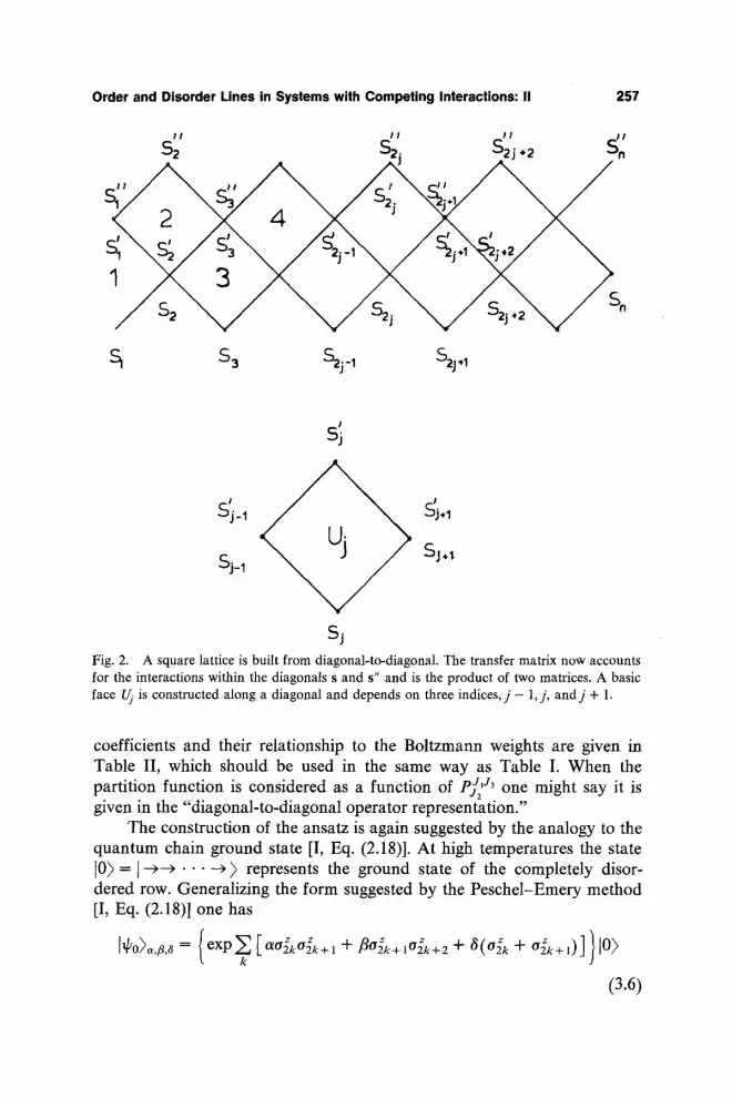
Suppose one builds up the square lattice from diagonal to diagonal, as shown in Fig. 2. First one adds the faces 1, 3 . . . . . n - 1 (n is even) and one moves from the diagonal s to the diagonal s'. This is represented by the matrix

W = U I U 3 , . . U n _ 1 ( 3 . 1 )

Then one adds the faces 2 , 4 , . . . , n, between the diagonal s' and the diagonal s". The corresponding matrix is

V= U2U4... U, (3.2)

The full diagonal-to-diagonal transfer matrix is given by (5)

T ~ VW (3.3)

where

(Uj-)s,s , = 8s],s,l . . . 8 S j _ l , s j _ W ( S j _ l , S j , S j + l [ S j _ l , S j , S j + l ) ~ s j . . , s j + o . . 8sn,sf, ( 3 . 4 )

and represents the j th face added as shown in Fig. 2. Note that Uj is diagonal in the j - 1, j + 1 indices. A representation-independent operator form is obtained by expanding Uj in a set of Pauli matrices as follows:

4 4 4 /" ~G , O ,O , ,,s,+, is; = g Z E (3.5)

J l =3 3"2 = 1 J3=3

This expansion has the same interpretation as Eq. (2.11). The sum over J1 and J3 is restricted to the diagonal matrices o 3 and 0 4 because Uj is diagonal in indices j - 1 and j + 1. In total there are 16 pJJ3 expansion


11 I I I I I I

$2 S2j S2 j . , Sn

11 I I I I

r~ s 3 s2j_~ s2j.~

I Sj

Sj'_I Sj.1

Sj_~ S j .

Sj Fig. 2. A square lattice is built from diagonal-to-diagonal. The transfer matrix now accounts for the interactions within the diagonals s and s" and is the product of two matrices. A basic face Uj is constructed along a diagonal and depends on three indices, j - 1,j, andj + 1.

coefficients and their relationship to the Boltzmann weights are given in Table II, which should be used in the same way as Table I. When the partition function is considered as a function of pf,.t3 one might say it is given in the "diagonal-to-diagonal operator representation."

The construction of the ansatz is again suggested by the analogy to the quantum chain ground state [I, Eq. (2.18)]. At high temperatures the state [0) = ] ~ - " ~ ) represents the ground state of the completely disordered row. Generalizing the form suggested by the Peschel-Emery method [I, Eq. (2.18)1 one has

__( z I~o>~,B,~ exp [~176 + fl~ 2k+2 + 8(02~ + Ozk+l)] IO>

(3.6)

ol

o0

Ta

ble

II

. T

he

R

ela

tio

ns

hip

b

etw

ee

n

the

We

igh

ts

Uj( s

j _ t,

sj ,

sj +

i [ sj

_ l,

sj_

l, "~

j--

"f' t,

:/+

t) a

nd

th

e

Ex

pa

ns

ion

C

oe

ffic

ien

ts

pJJ3

as

Giv

en

b

y E

q.

(3.5

). T

he

W

eig

hts

w(

sj_

j,sj

j sj

1,sj

) A

re A

lso

Sh

ow

n.

Th

e

Arr

ow

s

Ind

ica

te

the

N

on

ze

ro

PJ2 ~

s3 C

oe

ffic

ien

ts

in t

he

Ev

en

in

tera

cti

on

M

od

el.

Th

e

Co

rre

sp

on

din

g

Eigh

t-Ve

rtex

W

eig

hts

A

re

Dis

pla

ye

d

As

We

ll.

U

w

4,

$ $

$ $

$ $

4,

p133

p1

34

p43

p144

p2

33

p234

p4

3 p2

44

p333

p3

4 e~

3 ff3

44

p433

p4

34

p443

p4

44

++

+[+

++

+

+

I +

----

[++

--

+--

-+

--[-

---+

--

+

++

--[+

---

++

--

-+l-

-++

--

--

+-+

t+-+

+

-,-

--+

I

+-

--+

++

--

-- -

- ..{

-

+-+

_

..]- _

++

+

-++

.+

,---

++

1

:+--

3

--

+ _-

{-

_ _

---

4 --

+

++

--

_

+ 2

+--

++

- +

+

+--

5

---+

..

..

-I-

++

+

+--

+

+

7 +

+ +

+ --

--

+ --

+-+

+

+[-

+

8 +

+

--+

--

----

I+--

-t

- --

-++

-+

[++

6

+--

--

+--

I---

-

--

+ --

+

--

+

+ +

+ +

--

_

--

+ +

- +

--

+ +

--

_ +

+

+ +

+ +

+

--

+ --

+

+ --

+ +

..

..

--

+ +

--

_ +

+ +

+ +

+ +

+ +

--

+ +

--

+ --

_

+

..

..

+

+ +

+

+ --

_

+ +

--

_ +

--

+ --

+

--

+ --

+

+ +

..

..

+

+

_ _

+ +

--

_ +

+

+ --

+

--

_ +

- +

i i

:0

:3


where

10)= ~ I s , ) i s2 ) . . . { sN) (3.7) (sj= • 1)

Again, the exponential form of the ansatz and the Perron-Frobenius theorem (1~ ensures that (3.6) is a good candidate for the eigenvector associated with the largest eigenvalue. Following the definition of T DD (3.3) one requires that

and (3.8)

leading to

TDDI~o),,,#,O = ~kltP0)~,B,8 , )~ = X~)~

Restricting the discussion to symmetric matrices

(3.9)

U j ( j - 1, j + 1) = Uj(j + 1 , j - 1) (or P~d3 = PS3J'3) (3.10)

one has a = fl and the state (3.6) is an eigenstate provided

= e x p [ - a ( o f _ , o ; + ojzoj+l) - - 801] Uj exp[ a(oj_,oj z + ofoj+t) + 8o1]

(3.11)

is independent of o~'s when acting on the [0) state. This implies that the coefficients of the operators o/_ 1, o/ , of_ lof, of_ lof+ 1, and of_ lo/of+ l must be zero. Even after using two equations for fixing the parameters a and 8, there are still three equations left, restricting strongly the dimension of the disorder subspace if there is such a solution at all. Additional symmetries improve the situation. For the even (eight-vertex) model, for example, one has only two equations and one free parameter, a (8 = 0 in this case). This is not just a lucky coincidence. Actually, by introducing the bond Pauli as for the quantum chain [I, (2.12)]:

%,/2 =

k<j

(3.12)

the operator w(j, j + 1) [Eq. (2.11)] is mapped into the operator Uj+ 1/2 and the ansatz (2.14a, b) (t~p+) + I~p_ )) into the ansatz [~Po) .... 0 of Eq. (3.6). To make this relationship even more transparent one introduces the following

260 Rujan

parametrization:

p433 = AJ

e?3= - d ( 1 - "y)

P144 = J(1 + y) (3.13)

P334= h

p#4 = _ k

Solving Eqs. (3.9) one obtains that in this parametrization one recovers exactly the equations (2.24)-(2.29)! The only difference is that now the multicritical points (2.29) are from the same universality class as the T = 0 multicritical points of the ANNNI model (for details see I, Section 3). Furthermore, when expressing the free-fermion condition (2.30) using Table II one gets

p33p444 -I- p 3 3 p r 34 43. p34p43 = P2 P2 + (3 .14)

Again, for A = 0 one recovers from (3.13) and (3.14) the disorder surface (2.27).

,

w( sl,s21sl,s'z) = exp[ -~ ( sls2

I S,

A N E X A M P L E A N D C O N C L U S I O N S

For example, consider the model shown in Fig. 3:

+ s~s' 2 + sis I + s2s~) + Msls ' 2 + Ls2s' 1 ] I

El2 S 2

- / \ \

K/2 \ K/2

\\L \

\

(4.1)

$1 K / 2 $2 Fig. 3, The Ising model with next-neighbor and diagonal interactions.


This is an Ising model with n.n. interactions and diagonal (n.n.n.) competing interactions. This model has been proposed as a symmetrized version of the ANNNI model for K > 0, M > 0, L < 0 and is supposed to share many of its properties, including the presence of an incommensurate phase. (11) For K > 0, L = M < 0 the model (4.1) has a critical line with continuously changing exponents. (12)

Consider first the disorder lines. Using Table II one gets

p33 = e-Msinh(L) = - J(1 - y)

P ~ = e-Mcosh(L) = J(1 + V)

p34 = p43 = 0 (4.2)

P334= P343 = �89 = h

P433 = �89 (eM+Lcosh2K -- e M-c) = AJ

p444 = I (eM+Lcosh2K + e M-c)

and the disorder surface is given by Eq. (2.27). The lines of multicritical points are given by Eqs. (2.29) and in general involve that one or more coupling constants are infinite, so that T = 0.

Next consider the order lines. In this case the w ( j , j + I) matrix is symmetric only if L = M. Using Table I one obtains

P, , = e-Xcosh(K - 2L) = h , f

P22 = e-gsinh( K -- 2L) = f(-~ - l)

e l 4 = e41 = 1 = f f (4.3)

P23 = P32 = ]~ --- 0

P33 = eKsinh( K + 2L) = ] (1 + "7)

P44 = eXcosh( K + 2L)

and the order surface is given again by (2.17) but in terms of the J, /~, ~, and ff parameters. One concludes that the model (4.1) with M = L < 0 has both order and disorder lines at the same time. This is the consequence of the rotational symmetry of w(j, j + 1).

In conclusion, in this paper I have introduced a simple method for solving exactly the general IRF model along order and disorder trajectories. It turns out that the row-to-row transfer matrix formalism offers the possibility of calculating the free energy and correlation functions along the order trajectory, while the diagonal-to-diagonal transfer matrix allows for

262 Rujan

the search of disorder trajectories. This latter method can be applied also to staggered IRF models.

The generalization of these results to q-state spins is also possible and will be considered in the next paper of this series.

ACKNOWLEDGMENTS

I am grateful to G. Mtiller for the preprint ~4) and to F. Y. Wu for helpful suggestions.

REFERENCES

1. P. Ruj~-n, preceding paper, this issue. 2. I. Peschel and V. J. Emery, Z. Phys. B 43:241 (1981). 3. For a review see P. W. Kasteleyn, in Fundamental Problems in Statistical Physics, Vol. 3,

E. D. G. Cohen, ed., North-Holland, Amsterdam (1975). 4. J. Kurman, H. Thomas, and G. Mfiller, Physiea A, to be published. 5. R. J. Baxter, in Fundamental Problems in Statistical Physics, Vol. 5, E. D. G. Cohen, ed.,

North-Holland, Amsterdam (1980). 6. R. J. Baxter, o r. Stat. Phys. 15:485 (1976); 17:1 (1977). 7. For a review and earlier references see E. H. Lieb and F. Y. Wu, in Phase Transitions and

Critical Phenomena, Vol. II, C. Domb and M. S. Green, eds., Academic Press, London (1972).

8. C, A. Hurst and H. S. Green, J. Chem. Phys. 33:1059 (1960); C. Fan and F. Y. Wu, Phys. Rev. 179:560 (1969).

9. R. J. Baxter, J. Phys. A 13:L61 (1980). 10. O. Perron, Math. Ann. 64:248 (1907); S. B. Frobenius, Pressus. Acad. Wiss., 471 (1908). 11. P. Ruj~n, Phys. Rev. B 24:6620 (1981). 12. J. Oitmaa, J. Phys. A 14:1159 (1981) and references therein.

order and disorder lines in systems with competing interactions: ii. the irf model

Documents