Optimizing Agent Placement for FlowReconstruction of DDoS Attacks

Omer DemirDept. of Information Tech.Turkish National Police

Ankara, Turkiyeomerdemirkos@gmail.com

Bilal KhanDept. of Math & Comp. Science

John Jay College, CUNYNew York, USA

bkhan@jjay.cuny.edu

Ghassen Ben BrahimComputer Science Dept.Prince Mohamed Univ.

Al-Khobar, Saudi Arabiagbrahim@pmu.edu.sa

Ala Al-FuqahaComputer Science Dept.Western Michigan Univ.

Kalamazoo, USAala.al-fuqaha@wmich.edu

Abstract—The Internet today continues to be vulnerable todistributed denial of service (DDoS) attacks. We consider thedesign of a scalable agent-based system for collecting informationabout the structure and dynamics of DDoS attacks. Our systemrequires placement of agents on inter-autonomous system (AS)links in the Internet. The agents implement a self-organizingand totally decentralized mechanism capable of reconstructingtopological information about the spatial and temporal structureof attacks. The system is effective at recovering DDoS attackstructure, even at moderate levels of deployment.

In this paper, we demonstrate how careful placement ofagents within the system can improve the system’s effectivenessand provide better tradeoffs between system parameters andthe quality of structural information the system generates. Weintroduced two agent placement algorithms for our agent-basedDDoS system. The first attempts to maximize the percentage ofattack flows detected, while the second tries to maximize theextent to which we are able to trace back detected flows to theirsources. We show, somewhat surprisingly, these two objectives areconcomitant. Placement of agents in a manner which optimizesin the first criterion tends also to optimize with respect to thesecond criterion, and vice versa. Both placement schemes show amarked improvement over a system in which agents are placedrandomly, and thus provide a concrete design process by which toinstrument a DDoS flow reconstruction system that is effective atrecovering attack structure in large networks at moderate levelsof deployment.

Keywords—DDoS, network traffic, flow reconstruction.

I. INTRODUCTION

A denial of service (DoS) is the act of preventing service orshared resources (or services) from reaching legitimate users[10]. When a DoS attack is mounted from large numbers ofdistributed sources, it is termed a Distributed Denial-of-service(DDoS) attack. Arbor Network’s identifies DDoS as the mostcritical type of attack faced by Internet Service Providers [1].

The Internet architecture itself presents obstacles to theresolution of the DoS/DDoS problem. First, network linkresources are shared among all users, but there is no explicitenforcement of fair sharing. Second, core network componentsneed to be simple so they can quickly deal with very highvolumes of traffic. This in turn means they must do as littleas possible per packet, so the core is unable to providemuch security, implying that it is typically a service enforcedat the edges. Lastly, interconnected autonomous systems are

each managed by different authorities, and their heterogeneitymakes widespread deployment of defenses difficult. A moredetailed treatment of architectural features of the Internet andtheir implications for DDoS is given in [6]

Given the aforementioned inherent obstacles, the notionof “Solving the DDoS problem” has many interpretations.Here we focus on the problem of determining the true originsand mechanics of attacks. The source of attack packets isnot easy to identify because the IP header’s source addressmay be spoofed and network devices are not required to keepinformation about the path traveled by packets. We defineFlow Reconstruction as “Actions taken to find the true sourcesand/or routes of packets to a given destination”. There havebeen different approaches to this problem, including activelyinteracting with network traffic [5], [9], probabilistic andpacket marking techniques [2], [12], and hash based logging[13]. Next, we give a brief synopsis of prominent examples ofeach of these approaches:

Active Interaction is a strategy of interfering with attacktraffic to deduce information about attack sources based onthe systemic reaction to the interference. Backscatter is theprototypical example of this technique [9], operating at thelevel of BGP level routers. Backscatter finds the point of entryof the attack packets into BGP-level Internet backbone byhaving a backscatter server announce itself as the destina-tion for spoofed IPs being used as sources addresses in theattack. Then the destination network under attack is madeunreachable by having the backscatter server originate a BGProute announcement message. Since attackers continue to sendpackets to the victim but the target is no longer reachable, theingress routers reply with a “Destination unreachable” messageto the source IP of the attack packets. This ICMP messagegets delivered to the backscatter server, thus revealing theentry point of the attack packets into the backbone. Despiteits originality, Backscatter approach requires a modification tothe BGP protocol and suffers from a collateral effect wheregood traffic destined to the victim is being dropped at theBGP level.

Packet Marking relies on routers adding identificationinformation to the packets that they forward, so as to reveal thepath the packets have taken [2]. Marking every packet is notfeasible because of packet processing overhead introduced bychecksum recalculation. Probabilistic packet marking (PPM)circumvents this by having routers select which packets areto be marked randomly as they transit. Router information

978-1-4673-2480-9/13/$31.00 ©2013 IEEE 83

is written into the IP packet’s identification field (typicallyreserved for rebuilding fragmented packets). Whenever a routermarks a packet, information written there by previous routersis overwritten. If we can identify a packet that is markedby a router in a close neighborhood of the attacker, thenthe full reverse path can be reconstructed. The probability ofthe victim’s seeing a packet marked by the furthest router isp ·(1− p)(d−1), where p is the probability of marking a packetand d is the hop distance of the marking router. This techniquesuffers from both: packet processing load increase caused byoverloading the semantics of the IP packet fields and slow pathconvergence. Park and Lee [3] showed that PPM is effective atlocalizing the attack origin in single-source attacks but that asthe number of mounted attack sources increases, the tracebackis rendered more difficult.

Hash-Based Traceback was introduced by Snoeren andAlex [13], whose source path identification engine (SPIE)consists of data generation agents (DGA), SPIE collectionand reduction agents (SCAR), and SPIE traceback managers(STM). A DGA is the agent which calculates and storesthe packet digest in digest tables. To do this, it relies on kfixed hash functions of the infrequently changing fields of thepayload of each IP packet, with each function giving rise toan n bit number called a packet digest. The packets are storedin a space-efficient data structure called a Bloom filter [4] asfollows: Initially (and periodically thereafter) a 2n-sized bit-array is initialized to all zeros. As packets are received, kdistinct packet digests are computed and the correspondingbits in the array are set. When an IP Traceback request arrivesalong with the time and a copy of the packet that need tobe traced, the SCAR asks the routers, starting from the lastrouter, whether they have any record of the given packet. Thesequeries are answered by consultation with the router’s localBloom filter databases. If the indices in the array correspondingto the packet’s digests are not all set, then the packet has notbeen seen previously. Otherwise (all indices are set), then itis highly likely that the packet was seen earlier. The maindrawback of hash-based IP traceback is that in order to performtraceback, a copy of an attack packet must be presented tothe system as soon as the attack starts–since otherwise Bloomfilter tables might be discarded and the records lost. Therefore,some level of management and coordination between differentrouters and networks must exist.

Although there have been several approaches to flow re-construction, as described above, each presents drawbacks interms of requiring modification of existing Internet standards,increases in router processing load, or centralized coordinationor management.

Objectives. We sought to develop scalable system forcollecting information about the structure and dynamics ofDDoS attacks. The system must (1) self-organize and requireno centralized coordination, (2) effectively produce structuraland temporal data concerning DDoS attack flows, (3) beeffective even when system deployment levels are modest, (4)not significantly increase router processing load, (5) not requiremodification of router internals, and (6) be built using existingInternet protocols. An example of the kind of question we seekto be able to answer using the system is: What did the flow treestructure look like during the attack? The agent-based systemwe devised is able to answer such a question.

II. SYSTEM DESIGN

In this section we, informally describe the agent architec-ture and it main operation. A more detailed description at thelevel of finite state machines can be found in earlier workby the authors [8]. Each agent may be viewed as deviceswhich reside on inter-AS links. Each agent can (i) optionallyinject control traffic into the stream, (ii) passively listen toingress/egress traffic on a switch port and aggregate statisticsbased on the destination IP address of sampled packet headersset, and (iii) listen to all ICMP reply packets regardless oftheir destination. Whenever traffic volume to a destination IPtriggers an alarm function (e.g. exceeds a system threshold)the agent creates a Alert to Downstream (AD) message andsends it toward the victim. The AD message serves for 2purposes. It notifies the downstream agents about a potentialattack on a victim node and build an agent overlay networkin response to the attack by adding one more Logical Link(LL) to it. The AD message is sent as part of the payload ofthe ICMP reply packets destined to the victim IP address. TheTTL field in the AD message is initially set to 1 and graduallyincremented until an ACK from the next downstream node(toward the victim) is received. The TTL update process isterminated by the upstream agent node following the receiptof an ACK message originated by a node identifying itselfas the next downstream agent. Following this process, bothagents are ready to start sharing information about the attackon the victim over the newly added LL. The set of all LLs,together represents the structure of a distributed representationof a tree which is a maximal solution to the flow reconstructionproblem. Agents store their incident logical adjacencies in adistributed database that can be queried by sending broadcastmessages over the overlay network to determine the structureand dynamics of DDoS attacks. A detailed exposition of thesystem can be found in [7], [8].

Example. Figure 1 shows the reconstructed attack flowfollowing a DDoS attack. In this scenario, v is the victim,clouds numbered from 1 through 8 represent AS, A1 throughA4 are the attackers, circles are the routers, inter-AS linksare represented with solid lines. In this scenario, the attackpath is properly reconstructed in AS-8 despite the fact thatattack traffic from AS-3 came across non-participating AS-2. Attacks from AS-7 are traced only up to A-5. Tracebackare enabled to the possible extent through agent deployment.The reconstructed flows provide the victim with actionableinformation about both attack structure and dynamics.

III. MATHEMATICAL MODEL

In this section, we formally define the problem that agentsare trying to solve. This step is necessary to quantify theperformance of the solution quality of the proposed system.

A. Formal Statement of Problem and Solution

An instance of the flow reconstruction problem is a tuple(G,R,A,D,v) where G = (V,E) is a network on nodes V andE ⊂V ×V is a set of undirected edges between nodes.

A routing table is represented by the function R : V ×V → V , where R(u,d) = v is the next hop v on the pathfrom nodes u to d. set D ⊆ V is a set of attacking nodes

84

Fig. 1. Sample Flow Reconstruction

simultaneously attacking the victim node v ∈ V . The agentshave been deployed on a set of links A⊆ E.

To begin, we define flowstep f (d,v,n) for every non-negative integer n, inductively, by taking f (d,v,0) = d, andf (d,v,n+1) = R( f (d,v,n),v).

The flow from d toward v represents the sequence offlowsteps F(d,v) = ( f (d,v, i); i = 0,1, ...). A valid solutionis represented by a logical overlay network L = (S,ES) ona subset of agents S⊂ A where ES ⊂ S×S. Informally, (i) allagent nodes in the set S lies on the path from an attacker tothe victim. (ii) there is a LL in LS between 2 agents if bothagents appear successfully in the path from an attacker to thevictim. Formally:

• ∀e ∈ S⇒∃d ∈ D∧∃i ∈ N( f (d,v, i) = e)

• ∀(e,x) ∈ ES⇒∃d ∈ D∧∃i,k ∈ N such that◦ f (d,v, i) = e, and f (d,v,k) = x,◦ ∀ j ∈ (i,k) f (d,v, j) /∈ S.

Considering the above conditions

A solution L = (S,ES) is said to be maximum valid ifevery agent through which an attacker-originated flow transits,appears in S. That is:

e ∈ A∧∃d ∈ D∧ i ∈ N∧ ( f (d,v, i) = e) ⇒ e ∈ S. (1)

In [7], the authors proved that there is a unique maximalvalid solution for the flow reconstruction problem. Accord-ingly, we define the solution function s which assigns to eachinstance (G,R,A,D,v) of the flow reconstruction problem thisunique maximal valid solution. Hereafter, we denote the uniquemaximum valid solution of (G,R,A,D,v) by s(G,R,A,D,v).

B. Performance Measures

A performance measure is a function that evaluates thequality of a solution (S,ES) with respect to a problem instance(G,R,A,D,v). We need to establish some preliminary notationsusing which we can define our performance measures. We be-gin by defining a function dG,R,v : V×V →N∪{∞}. Intuitively,dG,R,v(x,y) equals the number of hops that a packet takes toreach y when it is sent by x to v in graph G according torouting table R. Note that dG,R,v is not generally symmetric or

transitive, and hence does not define a metric on V . Now givenany Y ⊂V and x ∈V , we define the distance from x to Y

dG,R,v(x,Y ) = miny∈Y{dG,R,v(x,y)}. (2)

The set of undiscovered attackers U ⊂D is defined as the setof vertices for which dG,R,v(u,S) =∞. The discovered attackersare then the complement set D�U . With all this notation inhand, we are now ready to define two performance measuresby which to assess the quality of a solution with respect to aspecific problem instance. The undiscovered attacker rate

M1((G,R,A,D,v),(S,ES))de f=|U ||D|

. (3)

When M1 is zero, every flow from every attacker is interceptedand hence detected by some agent. When M1 is one, everyflow from every attacker is goes undetected by the agentsystem. Clearly, lower values of M1 are preferred. The meannormalized distance to discovered attackers

M3((G,R,A,D,v),(S,ES))de f=

1|D�U | ∑

d∈D�U

dG,R,v(d,S)dG,R,v(d,v)

(4)

When M3 is close to zero, every attacking flow that has beenintercepted by an agent has been intercepted close to theattacker. In this case, traceback succeeds in getting close tothe attack sources. When M3 is close to one, every attackingflow that is intercepted by an agent has been intercepted closeto the victim. In this case, traceback fails to reach the attacksource. Clearly, lower values of M3 are preferred.

Example. Considering the scenario in Figure 1, A1 isunfolded by the agent in 3, A2 is unfolded by the agent in1, A3 is unfolded by the agent in 5, and A4 is unfolded by theagent in 8. This makes |U |= 0. Since |D|= 4, in this exampleM1 = 0

4 = 0, resulting in all attackers being discovered.

Since dG,R,v(A1,S) = 0, dG,R,v(A1,v) = 3, dG,R,v(A2,S) =4, dG,R,v(A2,v) = 4, dG,R,v(A3,S) = 1, dG,R,v(A3,v) = 4,dG,R,v(A4,S) = 0 and dG,R,v(A4,v) = 3, it follows that M3 forthis example is M3 = 1

3 (03 +

44 +

14 +

03 ) =

512 is the normalized

distance to the discovered attackers.

C. Expected Performance Measures

Unfortunately, in practice, we do not know where theattackers D⊂V lie in G, nor do we know which victim theywill choose to target. DDoS attacks are frequently orchestratedby botnets, and thus involve arbitrary sets of attacking nodeslocated all over the Internet which collude to attack the chosenvictim. Because we do not know the locations of the attackersor victims, the M1 and M3 performance measures defined inthe previous section cannot be directly computed.

Considering our definition of undiscovered attack rate, weattempt deriving a performance metric E[M1] that dependsonly on G, R, and A. This metric captures the expectedfraction of attackers which will be discovered following theengagement of a set of nodes in attacking a victim node.

Note that the expected fraction of undiscovered attackersE[M1] on the triple (G,R,A), can be computed as:

∑D⊆V,|D|=1,v∈V

M1((G,R,A,D,v), s(G,R,A,D,v))|V |2

(5)

85

Similarly, instead of M3, we use the expected mean nor-malized distance to attacking nodes. This measure quantifiesthe answer to the following question: if a random collectionof attacking nodes were to attack a random victim, then onthe flows which were intercepted by our agents, what is theexpected value of the normalized distance from our agents tothe attackers? This quantity, expected normalized distance todiscovered attackers, denoted E[M3], may be computed fora triple (G,R,A) as follows:

∑D⊆V,|D|=1,v∈V

M3((G,R,A,D,v),s(G,R,A,D,v))|V |2 · (1−E[M1])

(6)

IV. AGENT PLACEMENT ALGORITHMS

We note that the two performance measures E[M1] andE[M3] defined in the previous section were functions of onlythe network G = (V,E), the routing table R, and the agent setA⊂ E. Thus, for a fixed network and routing table, these twomeasures E[M1] and E[M3] can serve to differentiate betweendifferent agent sets.

More concretely, given two equinumerous agent setsA1,A2 ⊂ E for which |A1|= |A2|= n, an assertion like

E[M1](G,R,A2)> E[M1](G,R,A1) (7)

can be interpreted as expressing the fact that placing n agentsaccording to the specification A1 yields a lower fraction ofundetected attack flows than placing the agents according tospecification A2. The placement A1 is thus better.

Now suppose we have a third agent placement A3of n agents (i.e. |A3| = n) for which E[M1](G,R,A1) =E[M1](G,R,A3) but

E[M3](G,R,A1)> E[M3](G,R,A3). (8)

This would imply that the two agent placement schemes A1and A3 discover the same fraction of attack flows, but for A3the normalized distance from intercepting agents to attack flowsources is smaller, thus A3 is better than A1 in this scenario.

In this paper we will describe two deterministic algorithmsfor placing agents in a network G (with routing table R).These algorithms are namely M1-Greedy and M3-Greedy.We will compare their performance relative to the expectedperformance of an adversary named Random, which placesagents randomly on network edges. In the next sections wewill describe each algorithm in detail.

Random. The Random agent placement algorithm servesas a baseline against which to compare our agent placementschemes. The Random placement algorithm takes as input thenetwork G = (V,E), the routing table R, and the number ofagents n which are to be placed. It operates by randomlyselecting an edge e∈ E which does not already have any agenton it, and places an agent on that link e. This is repeated untilthe desired number of agents have been placed in G.

M1-Greedy Algorithm. The M1-Greedy algorithm se-quentially places the specified number of agents, one by one, ina manner that greedily minimizes E[M1] at each step. Supposeagents 1, ..., i− 1 have been placed already. The algorithmplaces agent i as follows:

Fig. 2. Hypothetical initial agent placement.

• Create a map from E to natural numbers; initialize allentries to 0.

• For all possible attacker-victim pairs in V ×V , do thefollowing: Start from attacker, proceed hop by hopaccording to R. At each hop, if there is no agent onthe edge increment the number associated with theedge by 1. If there is an agent on the edge, continueon to the next attacker-victim pair.

• Return the edge associated with the highest value asthe placement for the next agent and add an agent onthat link.

M3-Greedy Algorithm. The M3-Greedy algorithm se-quentially places the specified number of agents, one by one, ina manner that greedily minimizes E[M3] at each step. Supposeagents 1, ..., i− 1 have been placed already. The algorithmplaces agent i as follows:

• Create a map from E to real numbers; initialize allentries to 0.

• For all possible attacker-victim pairs in V ×V , do thefollowing: Start from the attacker, and proceed hopby hop according to R. For each edge e that lies onthe flow from the attacker to f , compute the reductionin M3 that would be obtained by placing agent i one. Increment the number associated with e by themagnitude of the reduction obtained.

• Return the edge associated with the highest value asthe placement for the next agent and add an agent onthat link.

Figure 2 and 3 illustrates the behavior of two agentplacement algorithms in a graph G with a routing table R.Figure 2 shows the location of the already existing agent.Figure 3 shows that the M1 and M3 places agents on differentedges. M3 algorithm tries to minimize the expected differenceto an attacker and M1 algorithm tries to maximize the expectednumber of attackers.

V. RESULTS

A. Experiment 1

The purpose of the first experiment is to quantify howthe two agent placement algorithms perform at comparable

86

Fig. 3. Behavior of M1 and M3 Greedy placement of the 2nd agent.

-0.4

-0.2

0

0.2

0.4

0.6

0.8

1

1.2

1.4

0 0.05 0.1 0.15 0.2 0.25 0.3 0.35 0.4 0.45 0.5

E[M

1]

Agent Density

E[M1] vs Agent Density

M1 GreedyM3 Greedy

Random

0.2

0.3

0.4

0.5

0.6

0.7

0.8

0.9

1

0 0.05 0.1 0.15 0.2 0.25 0.3 0.35 0.4 0.45 0.5

E[M

3]

Agent Density

E[M3] vs Agent Density

M1 GreedyM3 Greedy

Random

Fig. 4. M1 (top) and M3 (bottom) versus Agent Density

deployment levels, both relative to each other, and relative tothe expected performance of the random placement scheme.

For this part of the research we carried out three ex-periments. Each experiment runs on the same Waxman [14]network of 200 nodes. The network is created by randomlyplacing nodes in a 2D plane and randomly selecting linksbetween nodes with respect to their Waxman probabilities(where the likelihood of having a link between two nodes isinversely proportional to their Euclidean distance) and buildthe routing table for the network using the Bellman-Fordalgorithm. For succinctness, we will hereafter refer to this typeof network as a Waxman network.

Within this Waxman network G = (V,E), we placed δ · |E|agents according to the M1-Greedy, M3-Greedy and Randomplacement schemes, where the agent density δ was varied from0.0 to 0.50 fraction of the links. For each value of δ , measuredboth E[M1] and E[M3] of the system.

Figure 4 (top) shows E[M1] versus agent density curves forRandom, M1-Greedy, and M3-Greedy algorithms. It shows thatM1-Greedy and M3-Greedy algorithms have similar perfor-

mance with respect to E[M1] under identical agent deploymentlevels. It also shows that for smaller agent densities, theresulting values for M1 and M3-Greedy algorithms are onefull standard deviation below the performance of the Randomagent placement algorithm. At 10% percent agent deployment,the expected value of E[M1] for a random placement is 0.71,while M1-Greedy and M3-Greedy achieve E[M1] values ofapproximately 0.30. This agent density is the point where thedifference between random and greedy algorithms is maximal.As agent density increases, the performance of the threealgorithms begin to coincide. This graph clearly shows that M1and M3-Greedy algorithms perform significantly better thanRandom placement of agents when we consider the E[M1]values.

Figure 4 (bottom) shows M3 versus agent density curvesfor Random, M1-Greedy, and M3-Greedy algorithms. Just asin Figure 4 (left) the M1-Greedy and M3-Greedy outperformRandom on the E[M3] measure. Curves for M1-Greedy andM3-Greedy decreases faster than the curve for Random. At19% deployment the E[M3] value of Random is 0.59 while itis 0.471 and 0.475 for M1-greedy and M3-Greedy respectively.At this deployment level, the greedy algorithms performsapproximately 20% better than Random. This performanceadvantage is maintained as deployment levels increase.

The results of Experiment 1 show that the M1 and M3-Greedy algorithms always perform better than Random. Moresurprisingly perhaps, they show that optimizing greedily withrespect to M1 is in concordance with optimizing with respectto M3. More precisely, a greedy placement of agents whichsought to optimize E[M1] tends to be a placement which isquite good with respect to E[M3] as well, and vice versa. Thetwo new algorithms we have developed yield very effectiveagent deployments, even at low agent densities: A 10% deploy-ment according to either of the proposed greedy algorithms candetect 70% of the attack flows (since E[M1]≈ 0.3) and traceback halfway to the attacking nodes (since E[M3]≈ 0.5).

B. Experiment 2

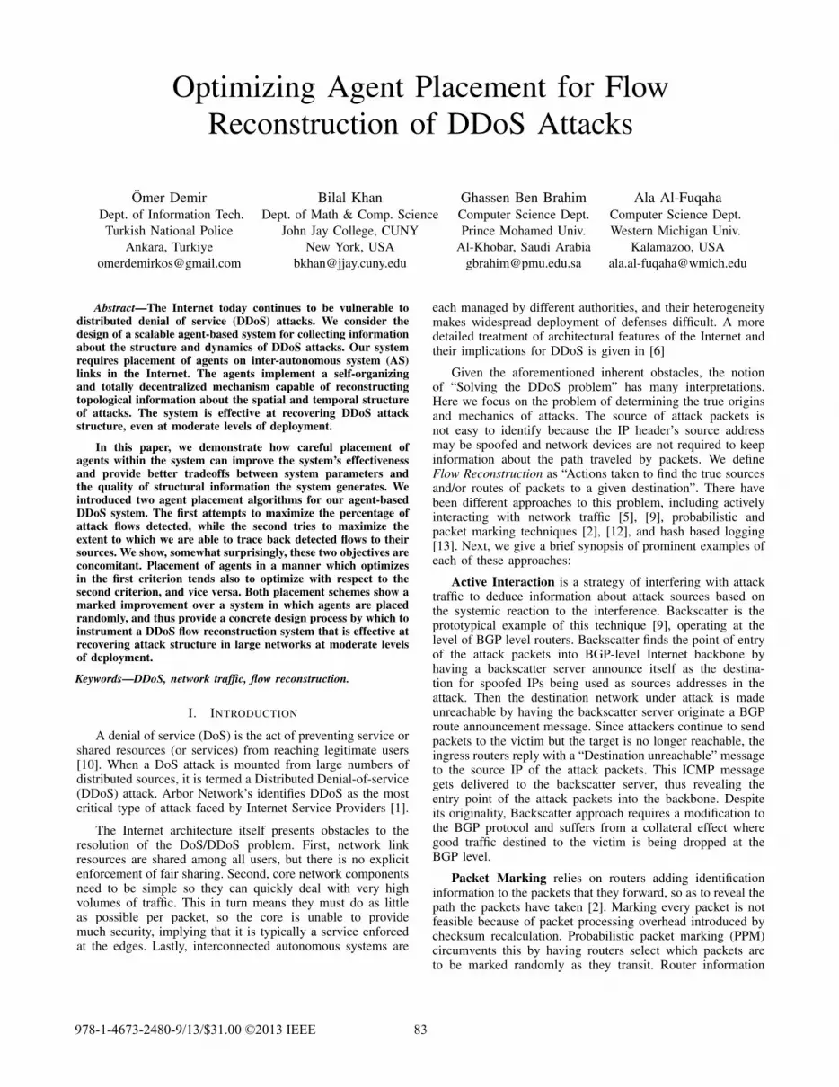
The purpose of the second set of experiments is to quantifythe extent to which our conclusions in experiment 1 might havebeen particular to the specific network in question. To judgethis, we repeated the same experiment with different networksby using different random number seeds when generating theWaxman network. Below we show the curves for just four ofthe networks, which were generated using random seeds 1, 2,3, and 4 respectively.

The top two graphs consider the performance of the M1-Greedy algorithm on different Waxman networks, while thebottom two graphs consider the performance of the M3-Greedy. The first and third graphs consider the E[M1] measure,while the second and fourth graphs consider the E[M3] mea-sure. As can be seen, the E[M3] measure is more sensitive tothe choice of network (i.e. random seed) than the E[M1] mea-sure. This is to be expected since E[M3] takes geometry anddistance into consideration, where E[M1] is only concernedwith geodesics (without reference to metrics). Also one cansee that the graphs in the top row exhibit the same sensitivityto the random seed, as the corresponding graphs in the bottomrow. This reflects the fact that the M1-Greedy and M3-greedy

87

0

0.1

0.2

0.3

0.4

0.5

0.6

0.7

0.8

0.9

1

0 0.05 0.1 0.15 0.2 0.25 0.3 0.35 0.4 0.45 0.5

E[M

1]

Agent Density

E[M1] vs Agent Density for M1-Optimizing Agent Placement

Seed: 1234

0.3

0.35

0.4

0.45

0.5

0.55

0.6

0.65

0 0.05 0.1 0.15 0.2 0.25 0.3 0.35 0.4 0.45 0.5

E[M

3]

Agent Density

E[M3] vs Agent Density for M1-Optimizing Agent Placement

Seed :1234

0

0.1

0.2

0.3

0.4

0.5

0.6

0.7

0.8

0.9

1

0 0.05 0.1 0.15 0.2 0.25 0.3 0.35 0.4 0.45 0.5

E[M

1]

Agent Density

E[M1] vs Agent Density for M3-Optimizing Agent Placement

Seed: 1234

0.3

0.35

0.4

0.45

0.5

0.55

0.6

0.65

0 0.05 0.1 0.15 0.2 0.25 0.3 0.35 0.4 0.45 0.5

E[M

3]

Agent Density

E[M3] vs Agent Density for M3-Optimizing Agent Placement

Seed :1234

Fig. 5. Simulation results of Experiment 2: Robustness

algorithms produce solutions that are comparable with respectto both the E[M1] and E[M3] measures (as was noted in theconclusion of Experiment 1).

The results of Experiment 2 indicate that conclusionsdrawn concerning the performance of the two schemes relativeto each other are robust against the specific choice of network(of fixed size). Knowing this, we can now proceed to considerthe impact of network size on the performance of the schemes.

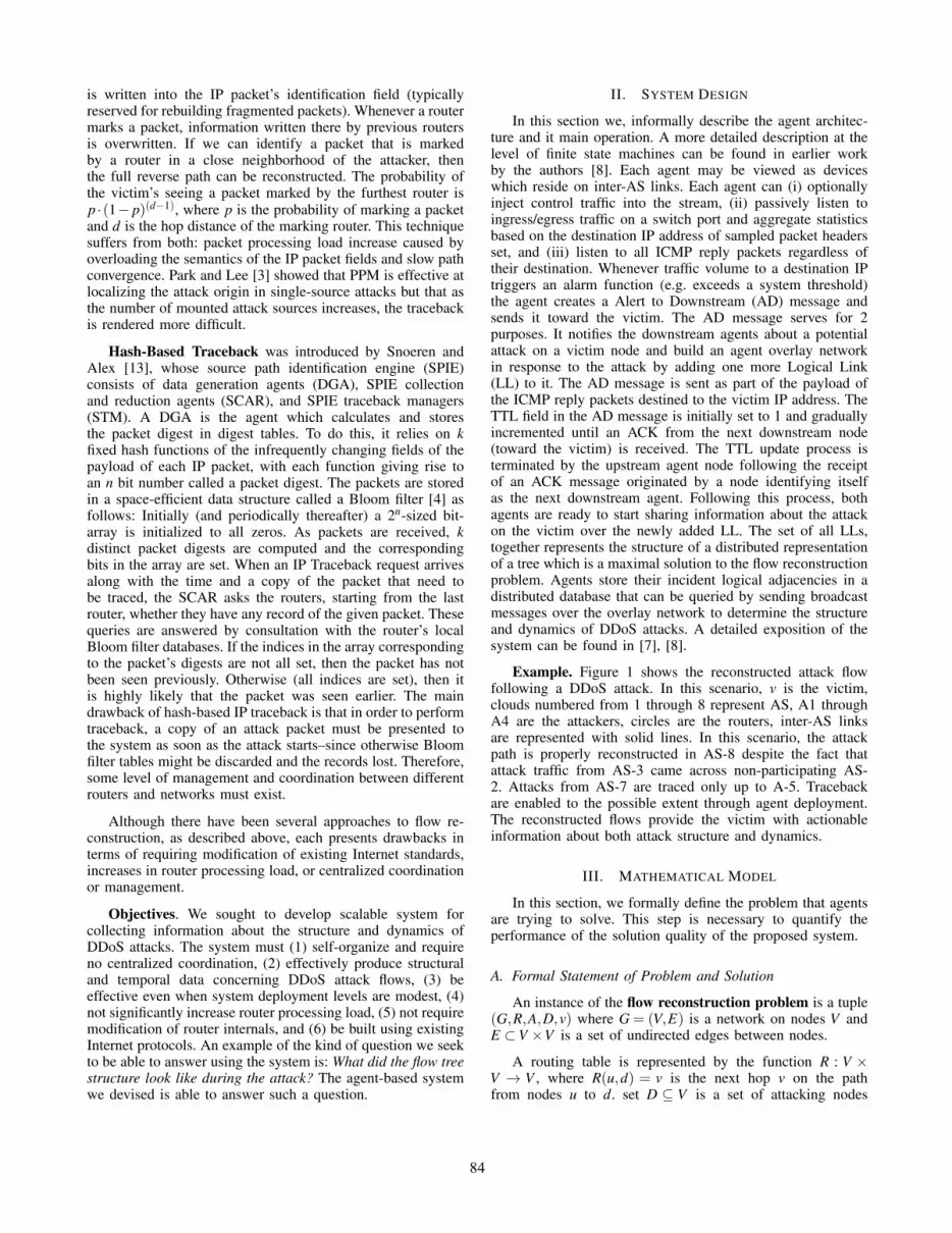
C. Experiment 3

The purpose of the third set of experiments is to quantifythe scalability of our conclusions with respect to network size.

0.1

0.2

0.3

0.4

0.5

0.6

0.7

0.8

0.9

0 0.02 0.04 0.06 0.08 0.1 0.12 0.14 0.16 0.18 0.2

E[M

1]

Agent Density

E[M1] vs Agent Density for Diff Net Sizes (M1 Optimizing Greedy)

# of nodes : 100200400800

0.42

0.44

0.46

0.48

0.5

0.52

0.54

0.56

0.58

0.6

0.62

0 0.02 0.04 0.06 0.08 0.1 0.12 0.14 0.16 0.18 0.2

E[M

3]

Agent Density

E[M3] vs Agent Density for Diff Net Sizes (M1 Optimizing Greedy)

# of nodes : 100200400800

0.1

0.2

0.3

0.4

0.5

0.6

0.7

0.8

0.9

0 0.02 0.04 0.06 0.08 0.1 0.12 0.14 0.16 0.18 0.2

E[M

1]

Agent Density

E[M1] vs Agent Density for Diff Net Sizes (M3 Optimizing Greedy)

# of nodes : 100200400800

0.44

0.46

0.48

0.5

0.52

0.54

0.56

0.58

0.6

0.62

0 0.02 0.04 0.06 0.08 0.1 0.12 0.14 0.16 0.18 0.2

E[M

3]

Agent Density

E[M3] vs Agent Density for Diff Net Sizes (M3 Optimizing Greedy)

# of nodes : 100200400800

Fig. 6. Simulation results of Experiment 3: Scalability

To determine this we carried out 8 experiments, which werelargely identical except for the Waxman network size. Here, wereport on the results of experiments on Waxman networks ofsizes 100, 200, 400, and 800 nodes, from which the reader canascertain nature of the relationship of the Greedy algorithm’sperformance advantage as network size increases.

The top two graphs consider the performance of the M1-Greedy algorithm on different Waxman networks, while thebottom two graphs consider the performance of the M3-Greedy. The 1st and 3rd graphs consider the E[M1] measure,while the 2nd and 4th graphs consider the E[M3] measure.

The first graph shows how the E[M1] curve changes when

88

the M1-Greedy algorithm is used to place agents in differentnetworks of different sizes. There are four curves in the graph,with each curve representing the results of the experimentfor networks of a different size (100, 200, 400, and 800respectively). Each of the curves individually shows similarcharacteristics. However, as the network size increases, wenote that the entire curve shifts downward. At an agent densityof 0.03 the E[M1] values for 100, 200, 400, and 800 nodenetworks are 0.704, 0.614, 0.526, 0.454 respectively. As thenumber of nodes in the network doubles, the E[M1] valuedecreases approximately 13%.

The second graph shows how the E[M3] curve changeswhen the M1-Greedy algorithm is used to place agents indifferent networks of different sizes. once Again four curves inthe graph represent the results of the experiment for networksof sizes 100, 200, 400, and 800 respectively. Each of the curvesindividually shows similar characteristics. Once again, as thenetwork size increases, we note that the entire curve shiftsdownward.

The third graph is very similar to the first one: It showshow the E[M1] curve changes when M3-Greedy algorithm isused to place agents in different networks of different sizes.For the agent density of 0.03 the E[M1] values for 100, 200,400, and 800 node networks are 0.696, 0.603, 0.510, 0.436respectively. As the number of nodes in the network doubles,the E[M1] value decreases approximately 14%. The graphshows us that the M3-Greedy agent placement performs betteras the net size gets bigger. Likewise, the fourth graph is similarto the second one: It shows how does the E[M3] curve behaveswhen M3-Greedy algorithm is used to place agents in differentnetworks of different sizes. Once again the graph shows thatas network size increases, the curve shifts downwards provingthe scalability of the proposed algorithm.

VI. CONCLUSION AND FUTURE WORK

We consider the design of a scalable agent-based systemfor collecting information about the structure and dynamicsof DDoS attacks. The agents implement a self-organizingand totally decentralized mechanism capable of reconstructingtopological information about the temporal and spatial struc-ture of attacks.

We showed that our system is effective at recovering DDoSattack flow structure, even at moderate levels of agent deploy-ment. We described two effective schemes for selecting theprecise locations at which agents should be placed: M1-Greedyand M3-Greedy. We quantified the performance of theseschemes and assessed their scalability. In experiment 1, we sawthat the greedy algorithms always perform significantly betterthan random placement, and provide good flow reconstructioncapabilities even at modest agent deployment densities. Wealso showed that the two optimization criteria (M1 and M3)are concomitant: optimizing one tends to optimize the other.In experiment 2 we saw that these conclusions were consistentacross different Waxman networks of the same size. Finally,in experiment 3 we saw that the effectiveness of the schemesactually improves as network size increases.

Future work. Having established that the greedy algo-rithms proposed here are effective at determining the place-ment of agents for optimal DDoS attack flow reconstruction,

we plan to use the proposed schemes to determine optimalplacement of agents within the real Internet topology, underat various deployment level assumptions. For this purpose weintend to use the inter-AS connectivity database maintainedby the CAIDA [11] project. Using the CAIDA topology wewill assess the extent to which the proposed system candeliver effective DDoS flow reconstruction services to theInternet community. This will enable us to determine thenecessary deployment level required in a real global system,and moreover, give us the precise inter-AS links on whichagents should be placed in order to maximize attack flowinterception and optimize traceback to attacking nodes.

REFERENCES

[1] Arbor Networks, http://www.arbornetworks .com[2] Bellovin, ICMP traceback messages, RFC draft, September http://tools.

ietf.org/draft/draft-be llovin-itrace/draft-bellovin-itrace- 00.txt (2000)[3] Bellovin, Cert advisory ca-1996-26, Cert Advisory, ‘http://www.cert.

org/advisories/CA- 1996-26.html (1996)[4] Bloom, B. H.: Space time trade-offs in hash coding with allowable

errors, Commun. ACM, vol. 13, no. 7, pp. 422–426, (1970)[5] Burch and Hal :Tracing anonymous packets to their approximate source,

Proceedings of the 14th USENIX conference on System administration.Berkeley, CA, USA: USENIX Association, 319–328 (2000)

[6] Demir O.: A Survey of Network Denial of Service Attacks andCountermeasures. City University of New York, Computer ScienceDepartment. (2009)

[7] Demir, O., Khan, B. : An Agent-based Architecture for Flow Re-construction of DDoS Attacks. Proceedings of Int. CommunicationsConference (ICC) 2010, Cape Town, South Africa, 23-27 (2010)

[8] Demir, O., Khan, B.: Quantifying Distributed System Stability throughSimulation A Case Study of an Agent-based System for Flow Re-construction of DDoS Attacks. In: Proceedings of the 1st IntelligentSystems, Modeling and Simulation Conference, Liverpool, England, 27-29 January (2010)

[9] Gemberling B., Morrow, C., and Greene, B.:ISP security-real worldtechniques. presentation, nanog. NANOG, www.nanog.org (2001)

[10] Gligor V.D.: A Note on Denial-of-Service in Operating Systems. IEEETrans. Softw. Eng. 10, 320–324 (1984)

[11] Hyun, Y., Huffaker, B., Andersen, D., Aben, E., Luckie, M., ClaffyK. C., and Shannon, C. The IPv4 Routed /24 AS Links Dataset -11/15/2009 , http://www.caida.org/data/active/ipv 4 routed topologyaslinks dataset.xml

[12] Savage, S, Wetherall, D. Karlin, A. and Anderson, T.: Practical networksupport for IP traceback, SIGCOMM Comput. Commun. Rev., vol. 30,no. 4, pp. 295–306, (2000)

[13] Snoeren, A. C.:Hash-based IP traceback, in SIGCOMM ’01: Proceed-ings of the 2001 conference on Applications, technologies, architec-tures, and protocols for computer communications. New York, NY,USA: ACM, pp. 3–14, (2001)

[14] Waxman, B. M.: Routing of Multipoint Connections.: BroadbandSwitching: Architectures, Protocols, Design, and Analysis. IEEE Com-puter Society Press, Los Alamitos, CA, USA (1991)

89