This article was downloaded by: [b-on: Biblioteca do conhecimento online IPC]On: 10 January 2013, At: 06:59Publisher: Taylor & FrancisInforma Ltd Registered in England and Wales Registered Number: 1072954 Registeredoffice: Mortimer House, 37-41 Mortimer Street, London W1T 3JH, UK

Communications in Statistics - Simulationand ComputationPublication details, including instructions for authors andsubscription information:http://www.tandfonline.com/loi/lssp20

Optimal Design of Acceptance SamplingPlans by Variables for NonconformingProportions When the StandardDeviation Is UnknownBelmiro P.M. Duarte a & Pedro M. Saraiva ba Department of Chemical and Biological Engineering, InstitutoSuperior de Engenharia de Coimbra (ISEC), Polytechnic Institute ofCoimbra, Coimbra, Portugalb GEPSI - PSE Group, Chemical Process Engineering and ForestProducts Research Centre (CIEPQPF), Department of ChemicalEngineering, University of Coimbra Pólo II, Coimbra, PortugalVersion of record first published: 10 Jan 2013.

To cite this article: Belmiro P.M. Duarte & Pedro M. Saraiva (2013): Optimal Design of AcceptanceSampling Plans by Variables for Nonconforming Proportions When the Standard Deviation Is Unknown,Communications in Statistics - Simulation and Computation, 42:6, 1318-1342

To link to this article: http://dx.doi.org/10.1080/03610918.2012.665548

PLEASE SCROLL DOWN FOR ARTICLE

Full terms and conditions of use: http://www.tandfonline.com/page/terms-and-conditions

This article may be used for research, teaching, and private study purposes. Anysubstantial or systematic reproduction, redistribution, reselling, loan, sub-licensing,systematic supply, or distribution in any form to anyone is expressly forbidden.

The publisher does not give any warranty express or implied or make any representationthat the contents will be complete or accurate or up to date. The accuracy of anyinstructions, formulae, and drug doses should be independently verified with primarysources. The publisher shall not be liable for any loss, actions, claims, proceedings,demand, or costs or damages whatsoever or howsoever caused arising directly orindirectly in connection with or arising out of the use of this material.

Communications in Statistics—Simulation and Computation R©, 42: 1318–1342, 2013Copyright © Taylor & Francis Group, LLCISSN: 0361-0918 print / 1532-4141 onlineDOI: 10.1080/03610918.2012.665548

Optimal Design of Acceptance Sampling Plans byVariables for Nonconforming Proportions When the

Standard Deviation Is Unknown

BELMIRO P.M. DUARTE1 AND PEDRO M. SARAIVA2

1Department of Chemical and Biological Engineering, Instituto Superior deEngenharia de Coimbra (ISEC), Polytechnic Institute of Coimbra, Coimbra,Portugal2GEPSI - PSE Group, Chemical Process Engineering and Forest ProductsResearch Centre (CIEPQPF), Department of Chemical Engineering, Universityof Coimbra Polo II, Coimbra, Portugal

This article presents an optimization-based approach for the design of acceptance sam-pling plans by variables for controlling nonconforming proportions when the standarddeviation is unknown. The variables are described by rigorous noncentral Student’st-distributions. Single and double acceptance sampling (AS) plans are addressed. Theoptimal design results from minimizing the average sampling number (ASN), subject toconditions holding at producer’s and consumer’s required quality levels. The problemis then solved employing a nonlinear programming solver. The results obtained are inclose agreement with previous sampling plans found in the literature, outperformingthem regarding the feasibility.

Keywords Acceptance sampling plans by variables; Nonconforming proportions; Non-linear programming; Unknown standard deviation.

Mathematics Subject Classification 62P30, 90C30, 90C90.

1. Introduction

Acceptance sampling (AS) is an effective quality control tool that has emerged in the pastdecades as one of the keystones of supplier–customer relationships (Evans, 2005). AS isessentially an auditing tool rather than a process development approach (Mitra, 1998),since it deals with the decision of accepting/rejecting a lot of items based on a sample.AS procedures can be applied to lots of items when testing reveals nonconformance ornonconformities regarding product functional attributes. It can also be applied to variablescharacterizing lots, revealing how far product quality is from specifications. Both ASapplications have the basic purpose of classifying a lot as accepted or rejected, given thequality level required. The advantages of AS plans by variables are related with lowersample sizes required to reach a given operating characteristic (OC) curve discrimination

Received November 24, 2009; Accepted February 6, 2012Address correspondence to Belmiro P. M. Duarte, Department of Chemical and Biological

Engineering, Instituto Superior de Engenharia de Coimbra (ISEC), Polytechnic Institute of Coimbra,Rua Pedro Nunes, 3030-199, Coimbra, Portugal; E-mail: bduarte@isec.pt

1318

Dow

nloa

ded

by [

b-on

: Bib

liote

ca d

o co

nhec

imen

to o

nlin

e IP

C]

at 0

6:59

10

Janu

ary

2013

Optimal Design of Acceptance Sampling Plans 1319

level compared with equivalent procedures for attributes (Schilling, 1982). This featureis particularly relevant when tests are destructive and the inspection cost is significant.However, AS plans by variables are often more difficult to implement, due to the lack ofknowledge to set the basic assumptions that have to be met. The implementation requiresdifferent procedures to check lots regarding each of the variables controlled and eachspecification. Seidel (1997) analyzed the pros and cons, and proved that sampling byvariables is optimal, and should be adopted whenever possible.

The design of AS plans by variables consists in the determination of the size of thesamples to inspect and of the acceptance threshold to accept/reject a lot, called acceptanceconstant (Duncan, 1974). The initial algorithms employed were based on the concept ofOC curve, using the risks of acceptance stipulated by the producer and the consumer tofind feasible combinations of parameters. Such designs result from the solution of theequations modeling the acceptance probability in the controlled points on the OC curve,corresponding to producer’s and consumer’s risks (Bowker and Goode, 1952). Taking ad-vantage of the growth of the calculation power in last decades, several algorithms weredeveloped to handle the problem computationally (see the work of Sommers (1981)). Sincethe system of algebraic equations resulting from controlling the quality levels stipulateddoes not have a closed form for double sampling plans, most of the algorithms developed tothis class of problems are based on enumeration techniques to seek feasible combinationsof variables (Hilbert, 2005; Sommers, 1981). The design of AS plans by variables whenthe standard deviation of the process is known is perfectly established in several qualitycontrol references (Duarte and Saraiva, 2010; Feldmann and Krumbholz, 2002; Schilling,1982). Those approaches assume that the statistic used for testing to reach the decision ofaccepting/rejecting the lot is normally distributed, and use the conditions at producer’s andconsumer’s quality levels to determine the sample size and the AS constant. Enumerativealgorithms allow to check the feasibility of the designs regarding both controlled pointsbut do not guarantee tighter solutions. To handle the problem in a systematic way, em-ploying mathematical programming approaches, Duarte and Saraiva (2010) proposed anoptimization-based framework relying on robust optimization solvers. The design problemis convex, and this strategy allows to reach optimal plans with respect to a given criterionwhile simultaneously satisfying the constraints.

The design of AS plans with unknown standard deviation is an open topic in AS the-ory. Most of the strategies used to deal with this case assume that the statistic employedfor testing follows an approximate normal distribution, instead of the noncentral Student’st-distribution, which indeed models the risk, to avoid the increase in the complexity of thecalculation. The design of double sampling plans by variables with unknown standard devi-ation was addressed by Krumbholz and Rohr (2006), who developed exact representationalforms for determining the OC curve.

In Section 2, we introduce the motivation for this work, particularly the findings ofthe infeasibility of AS plans available in the open literature for the case of σ unknown,designed assuming that noncentral Student’s t-distribution is approximated by normalapproximations proposed by Wallis (1947). Hamaker (1979) improved the approximationproposed by Wallis (1947). However, to compare our results with those of Sommers (1981),the former was considered.

Our analysis revealed that there is room to improve the design of AS plans for pro-cesses with unknown standard deviation by using the rigorous representation of the non-central Student’s t-statistic to generate the OC curve. Its use, enclosed in mathematicalprogramming-based approaches supported by robust optimization algorithms, guaranteesfeasible AS plans, thus producing designs that simultaneously and systematically address

Dow

nloa

ded

by [

b-on

: Bib

liote

ca d

o co

nhec

imen

to o

nlin

e IP

C]

at 0

6:59

10

Janu

ary

2013

1320 Duarte and Saraiva

both conditions at the points on the OC curve. The exact representation of the noncentralStudent’s t-statistic for single sampling plans relies on a series expansion developed duringthe decades of 1960–70. The design of double sampling plans involving bivariate noncen-tral Student’s t-distributions with different noncentrality parameters in both dimensionsis handled by employing the OC curve developed by Krumbholz and Rohr (2006), com-bined with numerical integration techniques. The optimization-based approach presented inDuarte and Saraiva (2010) for determining double AS plans for σ unknown by employingnormal approximations is extended to consider exact noncentral Student’s t-distribution.Similarly, the plans determined minimize the average sampling number (ASN), and thenoncentral Student’s t-cumulative distribution function (cdf) is computed via the algorithmof Lenth (1989), which stands in a series expansion of incomplete Beta functions.

The article is structured as following. Section 2 presents the basics of sampling theoryfor lot acceptance purposes. Section 3 presents the framework for designing single samplingplans by variables when σ is unknown. Section 4 extends the formulation to deal with doublesampling plans. Finally, Section 5 enumerates conclusions.

2. Acceptance Sampling Theory Basics and Motivation

To establish the nomenclature, we first introduce the conceptual basis of single AS plansby variables for controlling nonconforming proportions. We consider a system describedby a quality characteristic of a large-size lot of a given product, represented by X, withX ∼ N (μ, σ 2), where μ is the average and σ the standard deviation of X, with the valueof σ unknown, and thus approximated by the standard deviation of the sample, denoted ass. We also assume that there is a one-sided upper specification U > 0, with the proportionof nonconforming product, p, given as

1 − p = �

(U − μ

σ

), (1)

where �(x) stands for the cdf of the normal distribution N (0, 1) at x:

�(x) = 1√2 π

∫ x

−∞exp(−t2/2) dt. (2)

Here, we confine the strategy presented to AS plans for controlling quality variables with anupper specification. However, the extension to plans for variables with a lower specificationis straightforward. From Eq. (1), one obtains

zp = �−1(1 − p) = U − μ

σ, (3)

with �−1(1 − p) standing for the inverse of the cumulative standard normal distributionrepresenting a proportion 1 − p. We call the acceptance probability required at the qualitylevel p as P. The producer’s quality level is to be designated as p1, and the consumer’squality level as p2, with p1 < p2. Typical AS plans are designed to meet two simultaneousconditions, known as the OC curve two-point conditions:

1. The consumer accepts lots of quality level p1 no less than P1% of the times, withp1 called the acceptable quality level (AQL) and P1 represented by 1 − α.

Dow

nloa

ded

by [

b-on

: Bib

liote

ca d

o co

nhec

imen

to o

nlin

e IP

C]

at 0

6:59

10

Janu

ary

2013

Optimal Design of Acceptance Sampling Plans 1321

2. The producer accepts lots of quality level p2 no more than P2% of the times, withp2 called the limit quality level (LQL) and P2 represented by β.

In Section 3, we address the design of single sampling plans with a single specification,compactly represented as S1(ns1 ka), where ns1 ∈ N stands for the sample size and ka ∈ R

is the acceptance constant.The mechanics of the single sampling plan with an upper specification and σ unknown

is described as follows:

1. Sample ns1 items of a lot and determine the quality characteristic of each one,X1, . . . , Xns1 .

2. Determine the average, X, and the standard deviation, s, of the sample, where

X = 1

ns1

ns1∑i=1

Xi ; s =√∑ns1

i=1(Xi − X)2

ns1 − 1. (4)

3. Determine t1 = (U − X)/s.4. If t1 ≥ ka , accept the lot; otherwise, reject it.

The OC curve represents the acceptance probability of a lot, denoted as L(p), versusnonconforming proportion of the quality characteristic in the lot, denoted as p. Consideringthe mechanics of single AS plans presented above, L(p) = Pa(T1 ≥ √

nσ1 ka|p), with Pastanding for the acceptance probability, given a sampling acceptance constant, ka . The OCcurve for processes with σ known is defined by Eq. (5), and is represented in Figure 1:

L1(p) = �[√nσ1 (�−1(1 − p) − ka)], (5)

where nσ1 is the sample size for plans with σ known.Figure 1 also serves to graphically identify the quality levels and corresponding ac-

ceptance probabilities used for designing sampling plans based on the OC curve two-pointconditions paradigm, with the points denoted by (p1, P1) and (p2, P2), respectively.

For the case of σ unknown, the following is observed:√ns1

σ(U − X) ∼ N (

√ns1 �

−1(1 − p), 1), (6)

thus leading to√ns1

σ(U − X)

d= N (0, 1) + √ns1 �

−1(1 − p). (7)

Since (ns1 − 1) s2/σ 2 follows an independent χ2-distribution with ns1 − 1 degrees offreedom, the statistic

√ns1 (U − X)/s is described by noncentral Student’s t-distribution

with ns1 − 1 degrees of freedom and mean (also known as noncentrality parameter) equalto

√ns1 �

−1(1 − p). Therefore, the OC curve for this class of plans becomes

L2(p) =∫ +∞

√ns1 ka

ψ[T1|ns1 − 1,√ns1 �

−1(1 − p)] dT1

= 1 −∫ √

ns1 ka

−∞ψ[T1|ns1 − 1,

√ns1 �

−1(1 − p)] dT1 (8)

= [T1|ns1 − 1,√ns1 �

−1(1 − p)],

Dow

nloa

ded

by [

b-on

: Bib

liote

ca d

o co

nhec

imen

to o

nlin

e IP

C]

at 0

6:59

10

Janu

ary

2013

1322 Duarte and Saraiva

0 0.02 0.04 0.06 0.08 0.10

0.1

0.2

0.3

0.4

0.5

0.6

0.7

0.8

0.9

1

p1

1−α

P1

p2

βP

2

Quality level

Acc

epta

nce

prob

abili

ty

Figure 1. OC curve for single sampling plan S1(19 1.943).

where ψ[T1|ns1 − 1,√ns1 �

−1(1 − p)] is the noncentral Student’s t-probability den-sity function (pdf) with ns1 − 1 degrees of freedom and mean

√ns1 �−1(1 − p)

at T1, and [T1|ns1 − 1,√ns1 �−1(1 − p)] is the corresponding cdf. Due to the

complexity in determining noncentral Student’s t-statistic cdf, several authors usedan approximation based on the normal distribution N (μ + ka σ, σ 2 × (1/ns1 +k2a/(2 ns1 − 1))) proposed by Wallis (1947). The representational form of the OC curve

becomes

L3(p) = �{√ns1 [�−1(1 − p) − ka]|√ns1 ka, ns1

[1/ns1 + k2

a/(2 ns1 − 1)]}. (9)

Here, �(x|a, b) stands for the cdf of the normal distribution with average a and standarddeviation b at point x. A common strategy adopted to compute the OC curve representedby L3(p) (Schilling, 1982; Sommers, 1981) consists in using the form derived for the caseof σ known (Eq. 5), with nσ1 related to ns1 by

nσ1 = ns1

1 + k2a ns1/(2 ns1 − 1)

, (10)

which leads to

L3(p) = �

[√ns1

1 + k2a ns1/(2 ns1 − 1)

(�−1(1 − p) − ka

)]. (11)

Dow

nloa

ded

by [

b-on

: Bib

liote

ca d

o co

nhec

imen

to o

nlin

e IP

C]

at 0

6:59

10

Janu

ary

2013

Optimal Design of Acceptance Sampling Plans 1323

Here, Eq. (11) is also used for single AS plans with σ unknown. The computation ofthe cdf for noncentral Student’s t-statistic is performed using the algorithm of Lenth (1989),which, in its turn, is based on the expansion proposed by Guenther (1978).

Let us consider for the sake of simplicity that√ns1 ka ≥ 0. Therefore, the following

equality holds:

∫ √ns1 ka

−∞ψ[T1|ns1 − 1,

√ns1 �

−1(1 − p)] dT1

=∫ 0

−∞ψ[T1|ns1 − 1,

√ns1 �

−1(1 − p)] dT1

+∫ √

ns1 ka

0ψ[T1|ns1 − 1,

√ns1 �

−1(1 − p)] dT1, (12)

and the cdf calculation includes two terms, with∫ 0−∞ ψ[T1|ns1−1,

√ns1 �

−1(1−p)] dT1 =�[−√

ns1 �−1(1 − p)]:

[√ns1 ka|ns1 − 1,

√ns1 �

−1(1 − p)] = �[−√ns1 �

−1(1 − p)]

+∫ √

ns1 ka

0ψ[T1|ns1 − 1,

√ns1 �

−1(1 − p)] dT1. (13)

The second term is then approximated by an infinite-series expansion:

∫ √ns1 ka

0ψ[T1|ns1 − 1,

√ns1 �

−1(1 − p)] dT1

=+∞∑j=0

{rj Ix[j + 0.5, (ns1 − 1)/2] + qj Ix[j + 1, (ns1 − 1)/2]

}, (14)

Ix(a, b) = (a + b)

(a) (b)

∫ x

0T a−1

1 (1 − T1)b−1 dT1, (15)

rj = 1

2

exp(−δ2/2)

j !

(δ

2

)j, (16)

qj = 1

2√

2

exp(−δ2/2)

(j + 1.5)

(δ

2

)j, (17)

δ = √ns1 �

−1(1 − p), (18)

x = ns1 k2a

ns1 k2a + ns1 − 1

, (19)

where Ix(a, b) is the incomplete Beta distribution with (a, b) degrees of freedom at x and(a) is the function at a. The algorithm presented by Lenth (1989) to evaluate the integralof Eq. (14) stands on the addition of terms to the summation until a predefined accuracyis achieved. Since in our approach, the integral evaluation is enclosed in an optimizationproblem, the number of terms to include in the expansion is fixed a priori. Therefore, we

Dow

nloa

ded

by [

b-on

: Bib

liote

ca d

o co

nhec

imen

to o

nlin

e IP

C]

at 0

6:59

10

Janu

ary

2013

1324 Duarte and Saraiva

0 0.02 0.04 0.06 0.08 0.10

0.1

0.2

0.3

0.4

0.5

0.6

0.7

0.8

0.9

1

Quality level

Acc

epta

nce

prob

abili

tyσ knownσ unknown, Wallis approximationσ unknown, noncentral t distribution

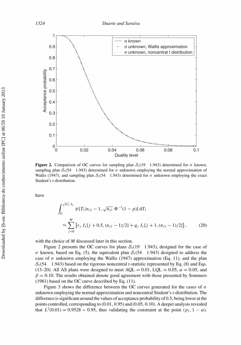
Figure 2. Comparison of OC curves for sampling plan S1(19 1.943) determined for σ known,sampling plan S1(54 1.943) determined for σ unknown employing the normal approximation ofWallis (1947), and sampling plan S1(54 1.943) determined for σ unknown employing the exactStudent’s t-distribution.

have ∫ √ns1 ka

0ψ[T1|ns1 − 1,

√ns1 �

−1(1 − p)] dT1

≈M∑j=0

{rj Ix[j + 0.5, (ns1 − 1)/2] + qj Ix[j + 1, (ns1 − 1)/2]

}, (20)

with the choice of M discussed later in this section.Figure 2 presents the OC curves for plans S1(19 1.943), designed for the case of

σ known, based on Eq. (5), the equivalent plan S1(54 1.943) designed to address thecase of σ unknown employing the Wallis (1947) approximation (Eq. 11), and the planS1(54 1.943) based on the rigorous noncentral t-statistic represented by Eq. (8) and Eqs.(13–20). All AS plans were designed to meet AQL = 0.01, LQL = 0.05, α = 0.05, andβ = 0.10. The results obtained denote good agreement with those presented by Sommers(1981) based on the OC curve described by Eq. (11).

Figure 3 shows the difference between the OC curves generated for the cases of σunknown employing the normal approximation and noncentral Student’s t-distribution. Thedifference is significant around the values of acceptance probability of 0.5, being lower at thepoints controlled, corresponding to (0.01, 0.95) and (0.05, 0.10). A deeper analysis revealedthat L2(0.01) = 0.9528 > 0.95, thus validating the constraint at the point (p1, 1 − α).

Dow

nloa

ded

by [

b-on

: Bib

liote

ca d

o co

nhec

imen

to o

nlin

e IP

C]

at 0

6:59

10

Janu

ary

2013

Optimal Design of Acceptance Sampling Plans 1325

0 0.02 0.04 0.06 0.08 0.1−5

0

5

10

15

20x 10

−3

Quality level

L2 (p)−

L3 (p)

OC curves difference

Figure 3. Difference between the OC curves for single sampling plan S1(54 1.943) obtainedemploying the noncentral t-distribution and the Wallis (1947) normal approximation.

However, L2(0.05) = 0.1057 > 0.10, thus violating the constraint at (p2, β). Therefore,we found that the AS plan based on the nonstandard normal distribution approximationis unfeasible. Afterward, our motivation will be to determine AS plans based on thenoncentral Student’s t-distribution to provide the research and industrial community withfeasible optimal solutions.

The motivating case just analyzed allows us to predict that feasible AS plans derivedbased upon the OC curve L2(p) would lead to larger sample size and/or larger AS constantthan those determined from L3(p).

The choice of the number of terms to include in the series expansion used to calculatenoncentral Student’s t-cdf is based on a heuristic rule. Lenth (1989) proved that 100 termsallow one to reach an accuracy of 10−6 for means ranging between –11.0 and 11.0. Here,the values of noncentrality parameter δ = √

ns1 �−1(1 − p) may be larger than 11.0, thus

requiring more than 100 terms. Figure 4 shows the values of rj , qj , Ix[j+0.5, (ns1 −1)/2],Ix[j + 1, (ns1 − 1)/2], and[

√ns1 ka|ns1 − 1,

√ns1 �

−1(1 −p)] forM = 150, ns1 = 54,δ = 14.278, and x = 0.7937. The terms that contribute more to the cdf are those arisingfrom j located in the neighborhood of M/2, and the contribution is neglectful for terms oforder higher than 130. Considering the results of Lenth (1989) and ours, one can adopt thefollowing heuristic:

M = ⌈ns1 k

2a

⌉, (21)

where • is the ceiling operator.

Dow

nloa

ded

by [

b-on

: Bib

liote

ca d

o co

nhec

imen

to o

nlin

e IP

C]

at 0

6:59

10

Janu

ary

2013

1326 Duarte and Saraiva

0 50 100 1500

0.005

0.01

0.015

0.02rj

qj

rj I

x[j+0.5,(n

1+1)/2]

qj I

x[j+1,(n

1+1)/2]

0 50 100 1500

0.2

0.4

0.6

0.8

1

j

Ix[j+0.5,(n

1+1)/2]

Ix[j+1,(n

1+1)/2]

cdf

Figure 4. Terms involved in the expansion used to calculate noncentral Student’s t-cdf.

3. Single Acceptance Sampling Plans

Considering the conceptual background introduced in Section 2, the design of single ASplans consists in the solution of an optimization problem aiming to minimize the samplesize, subject to the constraints in the controlled points on the OC curve. The problem,denoted as P1b, becomes

minns1,ka

ns1 (22)

s.t. L2(p1) ≥ 1 − α (23)

L2(p2) ≤ β (24)

Eqs. (13–19) (25)

ka > 0, ns1 ≥ 1,

where L2(p) is determined with the series expansion methodology presented in Section 2.The sample size is an integer variable, relaxed in problem P1b to avoid the need of usingmixed integer-nonlinear solvers and providing analytical derivatives of the incompleteBeta function in case integer variables are used. The integer solution for sample size isdetermined from the relaxed solution of P1b by rounding it to the upper integer value. Sincethe AS design problem is convex, the solution so obtained does not affect the feasibility ofthe plan. A similar approach is followed in all problems addressed.

To lower the computation time required to obtain the solution of the problem P1b,we first solve the equivalent problem based on the Wallis (1947) normal approximation,

Dow

nloa

ded

by [

b-on

: Bib

liote

ca d

o co

nhec

imen

to o

nlin

e IP

C]

at 0

6:59

10

Janu

ary

2013

Optimal Design of Acceptance Sampling Plans 1327

Table 1Single sampling plans for α = 0.05 and β = 0.1 (σ unknown) (values within parentheses

correspond to plans derived by Sommers (1981))

Wallis (1947) approximation Noncentral t-distribution

p1 p2 ns ka ns ka

0.02 0.030 835 (835) 1.957 (1.96) 837 1.9570.02 0.035 417 (417) 1.918 (1.92) 418 1.9190.02 0.040 259 (259) 1.883 (1.88) 260 1.8850.02 0.045 182 (182) 1.852 (1.85) 183 1.8540.02 0.050 137 (137) 1.824 (1.82) 138 1.8260.02 0.060 89 (89) 1.773 (1.77) 90 1.7770.02 0.070 65 (65) 1.729 (1.73) 65 1.7340.02 0.080 50 (50) 1.689 (1.69) 51 1.6960.02 0.090 41 (41) 1.653 (1.65) 41 1.6610.02 0.100 34 (34) 1.620 (1.62) 35 1.6290.02 0.110 29 (29) 1.589 (1.59) 30 1.6000.02 0.120 25 (25) 1.560 (1.56) 26 1.5720.02 0.130 22 (22) 1.533 (1.53) 23 1.5470.02 0.150 18 (18) 1.482 (1.48) 19 1.4990.02 0.170 15 (15) 1.436 (1.44) 16 1.4560.02 0.200 12 (12) 1.372 (1.37) 13 1.398

designated as problem P1a:

minns1,ka

ns1 (26)

s.t. L3(p1) ≥ 1 − α (27)

L3(p2) ≤ β (28)

ka > 0, ns1 ≥ 1.

The solution of P1a enables us to provide a feasible solution to handle the problem P1b

and simultaneously set the number of terms used in the series expansion, with M given byEq. (21).

Both optimization problems fall into the category of nonlinear programming (NLP).Here, they are solved employing GAMS/CONOPT, which is a robust solver to handlelarge-scale NLP problems based on a generalized reduced-gradient algorithm (Drud, 1985),included in the GAMS optimization platform. The relative and absolute tolerances are setto 10−6 in all optimization problems addressed in the article.

Table 1 compares the sampling plans atp1 = 0.01, α = 0.05, and β = 0.10, for severalvalues of LQL, available in the literature, with ours, obtained with noncentral Student’st-distribution. Our results require larger sample sizes (one additional item is required for allvalues of p2 simulated) and slightly larger values of ka . However, for single AS plans, thenormal distribution is a good approximation for the statistic modeling the lot acceptance

Dow

nloa

ded

by [

b-on

: Bib

liote

ca d

o co

nhec

imen

to o

nlin

e IP

C]

at 0

6:59

10

Janu

ary

2013

1328 Duarte and Saraiva

0 0.02 0.04 0.06 0.08 0.10

0.1

0.2

0.3

0.4

0.5

0.6

0.7

0.8

0.9

1

p1

1−α

P1

p2

βP

2

Quality level

Acc

epta

nce

prob

abili

tyWallis approximationnoncentral t distribution

Figure 5. Comparison of OC curves for sampling plans S1(137 1.824) based on the normal ap-proximation of Wallis (1947) and sampling plan S1(138 1.826) based on noncentral Student’st-distribution.

decision. This finding can be extended to the first stage of decision in double AS plans, oncethe numerical approach used to determine the acceptance probability is similar to ours.

The results presented here have the simple purpose of demonstrating the applicationof our strategy to single AS plans. Extensive tables can be easily generated by changing theparameters fixed. Figure 5 presents the comparison of OC curves for plans derived to meetAQL = 0.02, LQL = 0.05, α = 0.05, and β = 0.10. The OC curves are almost coincident,but the plan based on normal distribution leads to L2(0.02) = 0.9516 and L2(0.05) =0.1036, thus violating the constraint at p2. Both conditions hold for the plan based onnoncentral Student’s t-distribution with L2(0.02) = 0.9503 and L2(0.05) = 0.0998.

The comparison of plans based on noncentral Student’s t-distribution with those basedon the Wallis (1947) approximation reveals low advantages of the former, particularlyfor lower values of LQL. However, the use of rigorous representations avoids the risk ofdesigning unfeasible plans due to violations of the conditions in the controlled points.

4. Double Acceptance Sampling Plans

The design of double sampling plans, for the case of σ unknown, is represented asS2(ns1 kr1 ka; ns2 kr2), with ns1, ns2 ∈ N and kr1, ka, kr2 ∈ R, where ns1 is the sizeof the first sample, ns2 is the size of the second sample, kr1 is the rejection constant toachieve a decision based on the first sample (first stage of decision), kr2 is the rejectionconstant for deciding after the second sample is taken (second stage of decision), and ka is

Dow

nloa

ded

by [

b-on

: Bib

liote

ca d

o co

nhec

imen

to o

nlin

e IP

C]

at 0

6:59

10

Janu

ary

2013

Optimal Design of Acceptance Sampling Plans 1329

the acceptance constant to accept the lot based on the first sample (first stage of decision).The mechanics is as follows:

1. Sample ns1 items of a lot and determine the quality characteristic of each one,X1, . . . , Xns1 .

2. Determine the average, X1, and the standard deviation, s1, of the sample, byEq. (4).

3. Determine t1 = (U − X1)/s1.4. If t1 ≥ ka , accept the lot.5. If t1 < kr1, reject the lot.6. If kr1 ≤ t1 < ka , sample ns2 items of the lot and determine the quality characteristic

of each one, Xns1+1, . . . , Xns1+ns2 .7. Calculate the average of the second sample and the combined statistics:

X2 = 1

ns2

ns1+ns2∑i=ns1+1

Xi (29)

Xt = ns1

ns1 + ns2X1 + ns2

ns1 + ns2X2; st =

√∑ns1+ns2i=1 (Xi − Xt )2

ns1 + ns2 − 1. (30)

8. Determine t2 = (U − Xt )/st .9. If t2 ≥ kr2, accept the lot; otherwise, reject it.

4.1. Operating Characteristic Curve

The design of double AS plans for controlling nonconforming proportions has been ad-dressed by several authors by employing the OC curve concept, which requires expressionsto compute analytically or numerically the acceptance probability in both decision stages.The general representation of the OC curve is given by

L(p) = Pa(T1 ≥ √nσ1 ka) + Pa[(

√nσ1 kr1 ≤ T1 <

√nσ1 ka) ∧ (T2 ≥ √

nσ1 + nσ2 kr2)].(31)

For the sake of simplicity, Pa(T1 ≥ √nσ1 ka) is to be designated Pa1, denoting the ac-

ceptance probability of the lot based on the first sample, and Pa[(√nσ1 kr1 ≤ T1 <√

nσ1 ka) ∧ (T2 ≥ √nσ1 + nσ2 kr2)] as Pa2, representing the acceptance probability based

on the second sample. The acceptance probability of the second decision stage is definedin a bivariate region � = T1 × T2, with

� = {(T1, T2) ∈ R2 : (

√nσ1 kr1 ≤ T1 <

√nσ1 ka) ∧ (T2 ≥ √

nσ1 + nσ2 kr2)}. (32)

For the case of σ known, the OC curve is as follows (Bowker and Goode, 1952):

L4(p) = �[√nσ1 (�−1(1 − p) − ka)] +

∫ B

A

�

{√nσ1 + nσ2

nσ2

[√nσ1 + nσ2×

× (�−1(1 − p) − kr2

) +√

nσ1

nσ1 + nσ2t

]}d�(t)

dtdt, (33)

Dow

nloa

ded

by [

b-on

: Bib

liote

ca d

o co

nhec

imen

to o

nlin

e IP

C]

at 0

6:59

10

Janu

ary

2013

1330 Duarte and Saraiva

A = [kr1 −�−1(1 − p)]√nσ1, (34)

B = [ka −�−1(1 − p)]√nσ1, (35)

with the first term of L4(p) standing for Pa1 and the second for Pa2.For processes with unknown σ , the statistics

√ns1 (U − X1)/s1 and

√ns1 + ns2 (U −

Xt )/st follow noncentral Student’s t-distributions with different degrees of freedom andmeans. Furthermore, the distribution of

√ns1 + ns2 (U − Xt )/st depends on that of√

ns1 (U − X1)/s1. The computation of Pa2 is very demanding, since it involves thecalculation of the cdf for a bivariate noncentral Student’s t-distribution, here represented asϒ(m1, z1;m2, z2), where m1 and m2 are degrees of freedom in each dimension, and z1 andz2 are noncentrality parameters. For double AS plans, m1 = ns1 − 1, m2 = ns1 + ns2 − 2,z1 = √

ns1 �−1(1 − p), and z2 = √

ns1 + ns2 �−1(1 − p).

To lower the computational complexity of the design of double AS plans with σunknown, Sommers (1981) assumed that the statistic

√ns1 + ns2 (U − Xt )/st ∼ N (μ +

kr2 σ, σ2 × (1/(ns1 + ns2) + k2

r2/(2 ns1 + 2 ns2 − 1))). This assumption, based on theapproximation proposed by Wallis (1947), relates the total sample size for plans with σknown to the corresponding sample size for plans with σ unknown and simplifies thedetermination of acceptance probability Pa2:

nσ1 + nσ2 = ns1 + ns2

1 + k2r2 (ns1 + ns2)/(2 ns1 + 2 ns2 − 1)

. (36)

The works that use this strategy are not clear regarding the distribution that ap-proximates the statistic

√ns1 (U − X1)/s1, employed to model the acceptance proba-

bility in the first stage of decision. However, if one considers that√ns1 (U − X1)/s1 ∼

N (μ+ kr2 σ, σ2 × (1/(ns1) + k2

r2/(2 ns1 − 1))), similarly to what was assumed in Section3, the relations between each of the sample sizes required by plans for σ known and σunknown become respectively

nσ1 = ns1

1 + k2r2 ns1/(2 ns1 − 1)

, (37)

nσ2 = ns2

1 + k2r2 ns2/(2 ns2 − 1)

. (38)

The combination of Eqs. (36–38) with Eqs. (33–35) allows us to the derive the firstOC curve to represent double AS plans:

L5(p) = �[√nσ1 (�−1(1 − p) − ka)] +

∫ B

A

�

{√nσ1 + nσ2

nσ2

[√nσ1 + nσ2×

× (�−1(1 − p) − kr2

) +√

nσ1

nσ1 + nσ2t

]}d�(t)

dtdt, (39)

A = [kr1 −�−1(1 − p)]√nσ1, (40)

B = [ka −�−1(1 − p)]√nσ1, (41)

nσ1 = ns1

1 + k2r2 ns1/(2 ns1 − 1)

, (42)

Dow

nloa

ded

by [

b-on

: Bib

liote

ca d

o co

nhec

imen

to o

nlin

e IP

C]

at 0

6:59

10

Janu

ary

2013

Optimal Design of Acceptance Sampling Plans 1331

nσ2 = ns2

1 + k2r2 ns2/(2 ns2 − 1)

, (43)

nσ1 + nσ2 = ns1 + ns2

1 + k2r2 (ns1 + ns2)/(2 ns1 + 2 ns2 − 1)

. (44)

Another alternative addressed in this work consists in assuming that the statistic√ns1 (U − X1)/s1 ∼ N (μ + ka σ, σ

2 × (1/(ns1) + k2a/(2 ns1 − 1))). This assumption

leads to the following OC curve:

L6(p) = �[√nσ1 (�−1(1 − p) − ka)] +

∫ B

A

�

{√nσ1 + nσ2

nσ2

[√nσ1 + nσ2×

× (�−1(1 − p) − kr2

) +√

nσ1

nσ1 + nσ2t

]}d�(t)

dtdt, (45)

A = [kr1 −�−1(1 − p)]√nσ1, (46)

B = [ka −�−1(1 − p)]√nσ1, (47)

nσ1 = ns1

1 + k2a ns1/(2 ns1 − 1)

, (48)

nσ2 = ns1 + ns2

1 + k2r2 (ns1 + ns2)/(2 ns1 + 2 ns2 − 1)

− ns1

1 + k2a ns1/(2 ns1 − 1)

, (49)

nσ1 + nσ2 = ns1 + ns2

1 + k2r2 (ns1 + ns2)/(2 ns1 + 2 ns2 − 1)

. (50)

To address the problem of explicitly computing the OC curve based on the bivariatenoncentral Student’s t-distribution, Bowker and Goode (1952) derived closed-form formu-las, employed for designing plans at given combinations of AQL, LQL, α, and β. Theprocedure, standing on a rigorous treatment of noncentral Student’s t-statistics, was notable to cope with general AS plans because the geometry of the region�, used to computePa2, depends on the set of parameters to determine.

Assuming that X1 and Xt follow normal distributions and s1 and st are approximated byχ2r -distributions, where r is the number of degrees of freedom, Krumbholz and Rohr (2006)

proposed an ontological structure to rigorously determine Pa2. For each different classfound, corresponding to different features of the region �, the authors derived expressionsfor Pa2. The first step of the approach consists in finding the class corresponding to theplan to design. Afterward, the formula derived for such a class is used to compute Pa2,and subsequently, the OC curve. This strategy revealed that some of the double AS plansfound in the literature are unfeasible if rigorous noncentral Student’s t-distributions areconsidered. Indeed, constraint violations were detected at point (LQL, β).

In our work, we employ the strategy proposed by Krumbholz and Rohr (2006)and address the design of AS plans falling into the ontological class with kr1 > 0,ka

√ns1/(ns1 − 1) ≥ Q, and kr1

√ns1/(ns1 − 1) ≥ Q, with

Q =√ns1 (ns1 + ns2) k2

r2 − ns2 (ns1 + ns2 − 1)

(ns1 + ns2) (ns1 + ns2 − 1). (51)

Dow

nloa

ded

by [

b-on

: Bib

liote

ca d

o co

nhec

imen

to o

nlin

e IP

C]

at 0

6:59

10

Janu

ary

2013

1332 Duarte and Saraiva

The OC curve is therefore computed by

L7(p) = Pa1 + Pa2, (52)

where Pa1 = [√ns1 ka|ns1 − 1,

√ns1 �

−1(1 − p)], and the cdf of the noncentral Stu-dent’s t-distribution is computed through the series expansion methodology presented inSection 2. The term Pa2 is handled through the formulas proposed by Krumbholz andRohr (2006), combined with numerical integration techniques employed to compute thethree-dimensional integral term involved (Eq. 53). Considering the relations developed byKrumbholz and Rohr (2006), the acceptance probability associated with the second stageof decision is given by

Pa2 =∫ +∞

0

∫ a2(w1)

a1(w1)

∫ K(y)−w1

0{�[E2(w1, y,w2)] −�[E1(w1, y,w2)]}

× gns2−1(w2) × d�(y)

dygns1−1(w1) dw2 dy dw1, (53)

E2(w1, y,w2) = −D(y) +√H (w1, y,w2), (54)

E1(w1, y,w2) = −D(y) −√H (w1, y,w2), (55)

D(y) = A(y) B + k2r2 y (ns1 + ns2)

√ns1 ns2

B2 − ns1 (ns1 + ns2) k2r2

, (56)

H (w1, y,w2) = (ns1 + ns2)k2r2C(w1, w2) + k2

r2 ns2 (ns1 + ns2) y2 − [A(y)]2

B2 − ns1 (ns1 + ns2) k2r2

+ [D(y)]2,

(57)

A(y) =√ns1 + ns2 − 1 [

√ns1 y + (ns1 + ns2) �−1(1 − p)], (58)

B =√ns2 (ns1 + ns2 − 1), (59)

C(w1, w2) = (ns1 + ns2) (w1 + w2), (60)

K(y) = (ns1 + ns2) (ns1 + ns2 − 1)

ns1 (ns1 + ns2) k2r2 − B2

[y + √

ns1 �−1(1 − p)

]2, (61)

a1(w1) = kr1

√ns1

ns1 − 1

√w1 − √

ns1 �−1(1 − p), (62)

a2(w1) = ka

√ns1

ns1 − 1

√w1 − √

ns1 �−1(1 − p), (63)

where gr (z) is the value of the χ2-pdf with r degrees of freedom at z:

gr (z) = 1

2r (r/2)zr/2−1 exp(−z/2) (64)

and

d�(y)

dy= 1√

2 πexp(−y2/2). (65)

Dow

nloa

ded

by [

b-on

: Bib

liote

ca d

o co

nhec

imen

to o

nlin

e IP

C]

at 0

6:59

10

Janu

ary

2013

Optimal Design of Acceptance Sampling Plans 1333

The integration variables arew1, y, andw2, and univariate Gaussian quadrature formu-las are employed in each dimension. The upper limit of the outer integral is approximatedby a finite large value in order to avoid the finite-domain error, common in the applicationof numerical rules to infinite-domain integrals (Gelbard and Seinfeld, 1978). This error isdue to neglecting a part of the domain that contributes to the solution. Here, we set the upperlimit for the domain ofw1 to 2 ns1, considering that the maximum of a χ2

r -pdf occurs at r.

4.2. Problem Formulation

The strategy supporting the systematic design of double AS plans also stands on theminimization of the ASN, subject to the constraints in the controlled points on the OCcurve (Balamurali and Jun, 2007; Duarte and Saraiva, 2010). The ASN for double ASplans with σ known is given by the relation:

ASNσ = nσ1 + nσ2{�[√nσ1 (ka −�−1(1 − p))] −�[

√nσ1 (kr1 −�−1(1 − p))]}. (66)

Similar expressions can be derived for plans with σ unknown assuming normal distri-bution approximations. The value of ASNσ depends on the quality level used for itsdetermination, p. Sommers (1981) used the point (p1,AQL) for the calculation. Hamaker(1979) demonstrated that ASNσ curves are unimodal with a maximum located at pmax.Feldmann and Krumbholz (2002) derived a relation for the quality level corresponding tothe maximum of ASN:

pmax = 1 −�

(ka + kr1

2

). (67)

Based on this result, the authors used the quality level pmax to derive ASNσ , thus obtaining

ASNσ = nσ1 + nσ2

[2 �

(√nσ1

ka − kr1

2

)− 1

]. (68)

They also proved that the quality level pmax leads to minimal values of ASN, andthey determined double AS plans to address this criterion. The algorithm proposedwas denominated as ASN-minimax, and its application leads to plans with significantadvantages over the plans designed by Sommers (1981), since the values of ASNσ arelower for similar quality levels.

Here, the ASN-minimax criterion is also used as objective function. The equivalentASN for plans with σ unknown is denoted as ASNs . For AS plans standing on normal dis-tribution approximations, nσ1 and nσ2 are functions of ns1 and ns2, leading to problem P2a:

minns1,ns2,kr1,ka,kr2

nσ1 + nσ2

[2 �

(√nσ1

ka − kr1

2

)− 1

](69)

s.t. L5(p1) ≥ 1 − α (70)

L5(p2) ≤ β (71)

Eqs. (40–44) (72)

�−1(1 − p2) < kr1 ≤ kr2 ≤ ka < �−1(1 − p1), ns1, ns2, nσ1, nσ2 ∈ N.

This problem corresponds to the OC curve derived for√ns1 (U − X1)/s1 ∼ N (μ +

kr2 σ, σ2 × (1/(ns1) + k2

r2/(2 ns1 − 1))). The problem arising from the assumption that

Dow

nloa

ded

by [

b-on

: Bib

liote

ca d

o co

nhec

imen

to o

nlin

e IP

C]

at 0

6:59

10

Janu

ary

2013

1334 Duarte and Saraiva

√ns1 (U − X1)/s1 ∼ N (μ+ ka σ, σ

2 × (1/(ns1) + k2a/(2 ns1 − 1))) and

√ns1 + ns2 (U −

Xt )/st ∼ N (μ+ kr2 σ, σ2 × (1/(ns1) + k2

r2/(2 ns1 − 1))) is designated P2b:

minns1,ns2,kr1,ka,kr2

nσ1 + nσ2

[2 �

(√nσ1

ka − kr1

2

)− 1

](73)

s.t. L6(p1) ≥ 1 − α (74)

L6(p2) ≤ β (75)

Eqs. (46–50) (76)

�−1(1 − p2) < kr1 ≤ kr2 ≤ ka < �−1(1 − p1), ns1, ns2, nσ1, nσ2 ∈ N.

The integral terms involved in the OC curves of problems P2a and P2b are handledwith Gaussian quadrature formulas based on eight collocation points corresponding to thezeros of seventh-order Legendre polynomials (Abramowitz and Stegun, 1972).

To address the problem of determining ASNs when a rigorous noncentral Student’st-distribution is employed, Hilbert (2005) proposed

ASNs = ns1 + ns2{[

√ns1 ka|ns1 − 1,

√ns1 �

−1(1 − pmax)]−−[

√ns1 kr1|ns1 − 1,

√ns1 �

−1(1 − pmax)]}, (77)

and developed an approximation for pmax standing on the assumption that noncentralStudent’s t-distribution is well approximated by normal distribution:

pmax 1 −�

⎛⎝√

ns1

√2 ns1 + k2

r1 ka + √2 ns1 + k2

a kr1√2 ns1 + k2

r1 + √2 ns1 + k2

a

⎞⎠ . (78)

We will use Eq. (78) as an equality constraint to relate pmax with the sampling planparameters. The resulting optimization problem, designated as problem P2c, can thus beformulated:

minns1,ns2,kr1,ka,kr2

ns1 + ns2{[

√ns1 ka|ns1 − 1,

√ns1 �

−1(1 − pmax)]

−[√ns1 kr1|ns1 − 1,

√ns1 �

−1(1 − pmax)]}

(79)

s.t. L7(p1) ≥ 1 − α (80)

L7(p2) ≤ β (81)

kr1

√ns1

ns1 − 1≥

√ns1 (ns1 + ns2) k2

r2 − ns2 (ns1 + ns2 − 1)

(ns1 + ns2) (ns1 + ns2 − 1)(82)

Eqs. (13–20, 53–65, 78) (83)

�−1(1 − p2) < kr1 ≤ kr2 ≤ ka < �−1(1 − p1), ns1, ns2 ≥ 1.

The integration in the domains of w1 and w2 is carried out with Gaussian quadratureformulas based on 20 collocation points. The density of the grid used aims at guaranteeingnumerical accuracy for large domains, which may occur for particular parameter combi-nations. The integral in the domain of y is also computed through a Gaussian quadrature

Dow

nloa

ded

by [

b-on

: Bib

liote

ca d

o co

nhec

imen

to o

nlin

e IP

C]

at 0

6:59

10

Janu

ary

2013

Optimal Design of Acceptance Sampling Plans 1335

rule based on eight collocation points. The domains of inner integrals are dependent onw1, thus requiring the conformation of the numerical rules to the limits, which is done byredistributing the collocation points.

The plans proposed by Sommers (1981) were determined using normal Wallis (1947)approximations. The solution procedure used additional relations between the parametersto reduce the space of feasible solutions to enumerate, with the following assumptionsbeing made: (i) kr1 = kr2 and (ii) ns1 = ns2. AS plans without these constraints can easilybe designed, provided that efficient mathematical programming algorithms are employed.Moreover, plans designed without any constraint relating the parameters proved to outper-form plans determined considering additional constraints (Duarte and Saraiva, 2010). Thisresult was first observed by Feldmann and Krumbholz (2002), and of late by Duarte andSaraiva (2010). Both works proved that AS plans with unequal sample size and rejectionconstant (USS&RC) lead very often to lower values of ASNs . Here, it is assumed thatthe design of ASN-minimax plans does not involve any additional relation between theparameters.

The AS plans of Sommers (1981), based on equal values of ns1 and ns2, minimizethe administrative complexity. However, USS&RC plans allow to reach similar risks,minimizing the cost of sampling and testing because small sample sizes are required.

Problem P2c is much more complex than problems P2a and P2b due to the numericalrequirements needed to compute noncentral Student’s t-statistics. Its solution, involving amore complex objective function, additional variables, and equality constraints, increasesthe calculation efforts required. To improve the computational efficiency, we first solveproblem P2a to produce a feasible initial solution, subsequently provided to problem P2c,which is then solved also employing GAMS/CONOPT. The solution achieved fromP2a alsoallows us to set the number of terms to use in the calculation of the noncentral Student’st-cdf (Eq. 14), as well as the upper limit for the integral corresponding to variable w1

involved in the computation of Pa2.

4.3. Results

To demonstrate the robustness and accuracy of our approach, we determined the AS plansfor p1 = 0.02, α = 0.05, and β = 0.1, with p2 varying between 0.03 and 0.2. The rangeof cases considered aims mainly to compare the accuracy of our approach, combined withthe rigorous treatment of noncentral Student’s t-cdf, with the plans listed in Sommers(1981), determined assuming normal distribution approximations and enumerative solu-tion schemes. Extensive tables of plans can be produced by changing the producer’s andconsumer’s risks and quality level requirements.

Table 2 compares USS&RC plans, obtained with the L5(p) OC curve, with the plansof Sommers (1981). Our plans lead to larger values of ASNs because they use the qualitylevel pmax in the calculation instead of p1, used by Sommers (1981). The value of pmax forthe AS plan to meet AQL = 0.02, LQL = 0.05, α = 0.05, and β = 0.10 is 0.0340. Thevalue of ASNs based on the sample size of the corresponding plan proposed by Sommers(1981) for this quality level is 146.7, much larger than ours (117.6). Our approach leads to aconsistent trend in the acceptance and rejection constants, a decrease being observed as theLQL increases. Another point to stress is that our strategy does not require any additionalconstraint between the parameters.

Tables 3 and 4 show the plans designed with L6(p) and L7(p) OC curves, respectively.Both lead to larger values of ASNs than those required by plans based on L5(p), presented

Dow

nloa

ded

by [

b-on

: Bib

liote

ca d

o co

nhec

imen

to o

nlin

e IP

C]

at 0

6:59

10

Janu

ary

2013

1336 Duarte and Saraiva

Table 2Double sampling plans for α = 0.05 and β = 0.1 (σ unknown)

USS&RC plans based on L5(p) Sommers (1981) plans

p1 p2 ns1 ns2 kr1 kr2 ka ASNs ns1 kr1 ka ASNs

0.02 0.03 527 416 1.910 1.957 2.001 719.4 600 1.94 1.99 675.80.02 0.035 263 207 1.853 1.918 1.981 358.5 285 1.89 1.98 334.80.02 0.04 164 128 1.803 1.883 1.963 223.0 179 1.85 1.95 205.80.02 0.045 115 90 1.759 1.851 1.946 156.2 122 1.81 1.95 144.50.02 0.05 86 68 1.716 1.822 1.935 117.6 96 1.78 1.91 110.10.02 0.06 56 44 1.646 1.770 1.908 76.3 62 1.72 1.87 70.40.02 0.07 41 31 1.587 1.724 1.885 55.1 46 1.67 1.83 51.60.02 0.08 31 25 1.527 1.682 1.870 42.5 35 1.62 1.81 39.60.02 0.09 25 20 1.475 1.644 1.856 34.3 27 1.57 1.82 31.50.02 0.10 21 17 1.440 1.607 1.829 28.6 22 1.53 1.82 26.10.02 0.11 19 12 1.405 1.576 1.815 24.4 20 1.50 1.75 22.80.02 0.12 16 12 1.374 1.541 1.790 21.1 17 1.47 1.72 19.20.02 0.13 14 11 1.342 1.510 1.772 18.6 15 1.43 1.74 17.40.02 0.15 11 9 1.266 1.455 1.759 14.9 12 1.38 1.66 13.50.02 0.17 9 7 1.176 1.410 1.774 12.3 10 1.31 1.69 11.70.02 0.20 7 6 1.113 1.334 1.725 9.7 8 1.23 1.70 9.6

Table 3USS&RC double sampling plans based on L6(p) for α = 0.05 and β = 0.1 (σ unknown)

p1 p2 ns1 ns2 kr1 kr2 ka ASNs

0.02 0.030 541 406 1.909 1.958 2.000 727.70.02 0.035 273 200 1.851 1.920 1.978 364.40.02 0.040 172 122 1.800 1.886 1.958 227.70.02 0.045 121 86 1.754 1.855 1.941 160.10.02 0.050 92 64 1.712 1.827 1.924 121.00.02 0.060 61 40 1.638 1.777 1.895 79.00.02 0.070 45 28 1.575 1.733 1.867 57.50.02 0.080 35 22 1.519 1.695 1.841 44.60.02 0.090 29 17 1.474 1.659 1.812 36.20.02 0.100 24 14 1.411 1.626 1.806 30.30.02 0.110 21 12 1.388 1.597 1.766 25.90.02 0.120 18 11 1.339 1.569 1.755 22.60.02 0.130 16 9 1.283 1.541 1.753 20.00.02 0.150 13 7 1.203 1.492 1.728 16.20.02 0.170 11 6 1.166 1.448 1.671 13.50.02 0.200 9 5 1.137 1.389 1.576 10.7

Dow

nloa

ded

by [

b-on

: Bib

liote

ca d

o co

nhec

imen

to o

nlin

e IP

C]

at 0

6:59

10

Janu

ary

2013

Optimal Design of Acceptance Sampling Plans 1337

Table 4USS&RC double sampling plans based on L7(p) for α = 0.05 and β = 0.1 (σ unknown)

p1 p2 ns1 ns2 kr1 kr2 ka ASNs

0.02 0.030 532 408 1.912 1.958 2.003 718.60.02 0.035 275 198 1.862 1.920 1.978 360.00.02 0.040 166 129 1.810 1.887 1.966 224.20.02 0.045 115 93 1.764 1.857 1.956 157.30.02 0.050 85 72 1.722 1.829 1.949 118.80.02 0.060 57 47 1.660 1.781 1.923 77.30.02 0.070 42 33 1.602 1.738 1.907 56.20.02 0.080 33 25 1.551 1.701 1.896 43.60.02 0.090 27 21 1.505 1.666 1.888 35.30.02 0.100 22 17 1.465 1.635 1.876 29.60.02 0.110 19 15 1.428 1.606 1.868 25.30.02 0.120 17 13 1.393 1.579 1.863 22.10.02 0.130 15 11 1.363 1.554 1.855 19.60.02 0.150 12 9 1.307 1.507 1.846 15.80.02 0.170 11 8 1.256 1.465 1.841 13.30.02 0.200 9 6 1.191 1.408 1.833 10.6

in Table 2. The values of ASNs determined with the OC curve L7(p) fall within the rangeof the other two, both based on normal distribution approximations.

Figure 6 compares the OC curves of all plans determined for AQL = 0.02, LQL = 0.05,α = 0.05, and β = 0.10, which are quite similar. L7(p) leads to lower values of acceptanceprobability for higher nonconforming proportion values and overestimates the acceptanceprobability in the range of low values of p. A deeper analysis of the performance ofthe plans at the controlled points reveals that those resulting from L5(p) and L6(p) violatethe constraint at (LQL,β), an observation already made by Krumbholz and Rohr (2006).From a practical point of view, the impact of this violation is often disregarded, since thedifference is small. From a theoretical point of view, it deserves some attention because theplan based on L7(p) is the only one that systematically allows to meet the risks considered.Table 5 clarifies this finding and reveals that only the OC curve based on rigorous noncentralStudent’s t-distribution produces feasible plans for this case.

Table 5Performance of AS plans at the OC controlled points

OC curve Plan design L(p1) L(p2)

Based on Sommers (1981) S2(96 1.78 1.91; 96 1.78) 0.9533 0.1044∗

L5(p) S2(86 1.716 1.935; 68 1.822) 0.9553 0.1089∗

L6(p) S2(92 1.712 1.924; 64 1.827) 0.9586 0.1040∗

L7(p) S2(85 1.722 1.949; 72 1.829) 0.9503 0.0981

∗Constraint violation.

Dow

nloa

ded

by [

b-on

: Bib

liote

ca d

o co

nhec

imen

to o

nlin

e IP

C]

at 0

6:59

10

Janu

ary

2013

1338 Duarte and Saraiva

0 0.01 0.02 0.03 0.04 0.05 0.06 0.07 0.080

0.1

0.2

0.3

0.4

0.5

0.6

0.7

0.8

0.9

1

p1

1−α

P1

p2

βP

2

Quality level

Acc

epta

nce

prob

abili

tySommers planL5(p) based planL6(p) based planL7(p) based plan

Figure 6. Comparison of OC curves for double AS plans based on rigorous noncentral Student’st-distribution for AQL = 0.02, LQL = 0.05, α = 0.05, and β = 0.10.

Figure 7. Sensitivity analysis of double AS plans designed for AQL = 0.02, α = 0.05, and β = 0.10to LQL.

Dow

nloa

ded

by [

b-on

: Bib

liote

ca d

o co

nhec

imen

to o

nlin

e IP

C]

at 0

6:59

10

Janu

ary

2013

Optimal Design of Acceptance Sampling Plans 1339

0 0.01 0.02 0.03 0.04 0.05 0.06 0.07 0.080

0.1

0.2

0.3

0.4

0.5

0.6

0.7

0.8

0.9

1

p1

1−α

P1

p2

βP

2

Quality level

Acc

epta

nce

prob

abili

tyP

a1 with appr. normal dist.

OC curve with appr. normal dist.P

a1 with noncentral t dist.

OC curve with noncentral t dist.

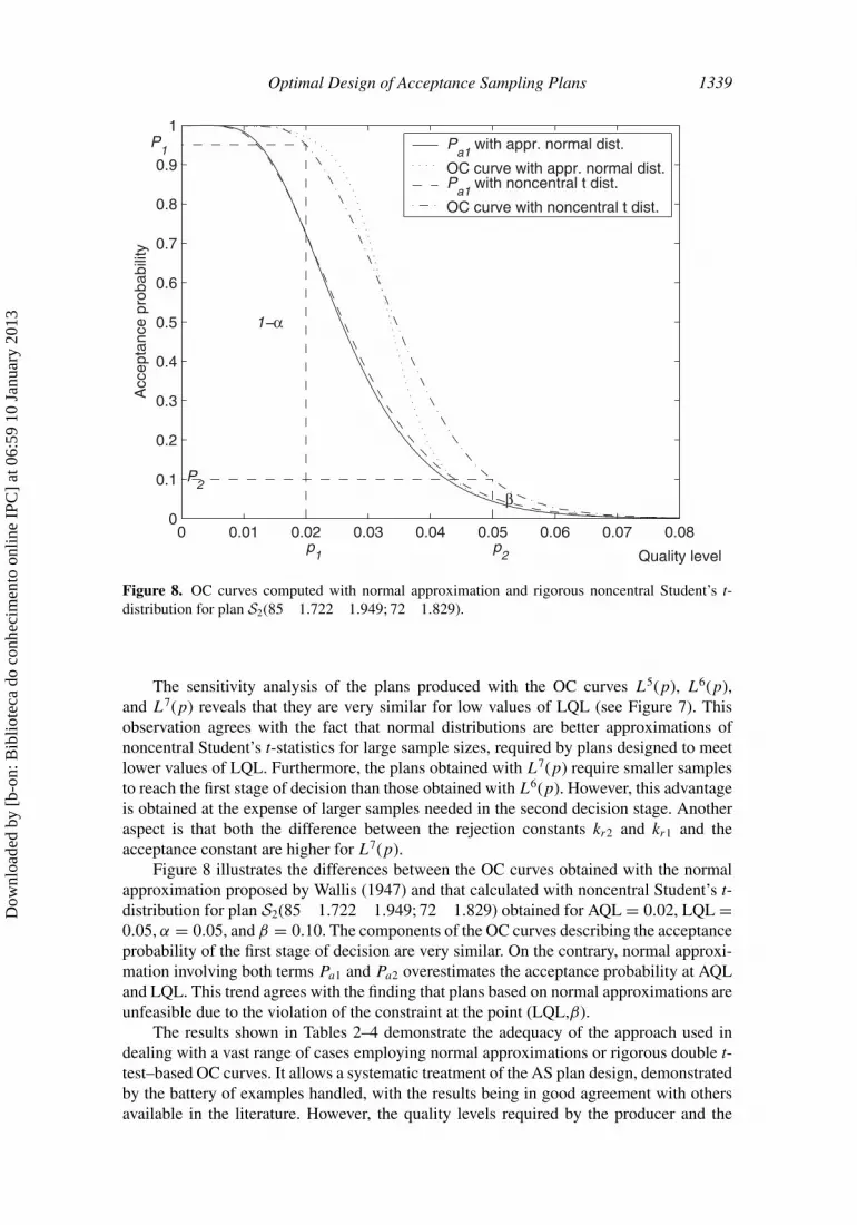
Figure 8. OC curves computed with normal approximation and rigorous noncentral Student’s t-distribution for plan S2(85 1.722 1.949; 72 1.829).

The sensitivity analysis of the plans produced with the OC curves L5(p), L6(p),and L7(p) reveals that they are very similar for low values of LQL (see Figure 7). Thisobservation agrees with the fact that normal distributions are better approximations ofnoncentral Student’s t-statistics for large sample sizes, required by plans designed to meetlower values of LQL. Furthermore, the plans obtained with L7(p) require smaller samplesto reach the first stage of decision than those obtained with L6(p). However, this advantageis obtained at the expense of larger samples needed in the second decision stage. Anotheraspect is that both the difference between the rejection constants kr2 and kr1 and theacceptance constant are higher for L7(p).

Figure 8 illustrates the differences between the OC curves obtained with the normalapproximation proposed by Wallis (1947) and that calculated with noncentral Student’s t-distribution for plan S2(85 1.722 1.949; 72 1.829) obtained for AQL = 0.02, LQL =0.05, α = 0.05, and β = 0.10. The components of the OC curves describing the acceptanceprobability of the first stage of decision are very similar. On the contrary, normal approxi-mation involving both terms Pa1 and Pa2 overestimates the acceptance probability at AQLand LQL. This trend agrees with the finding that plans based on normal approximations areunfeasible due to the violation of the constraint at the point (LQL,β).

The results shown in Tables 2–4 demonstrate the adequacy of the approach used indealing with a vast range of cases employing normal approximations or rigorous double t-test–based OC curves. It allows a systematic treatment of the AS plan design, demonstratedby the battery of examples handled, with the results being in good agreement with othersavailable in the literature. However, the quality levels required by the producer and the

Dow

nloa

ded

by [

b-on

: Bib

liote

ca d

o co

nhec

imen

to o

nlin

e IP

C]

at 0

6:59

10

Janu

ary

2013

1340 Duarte and Saraiva

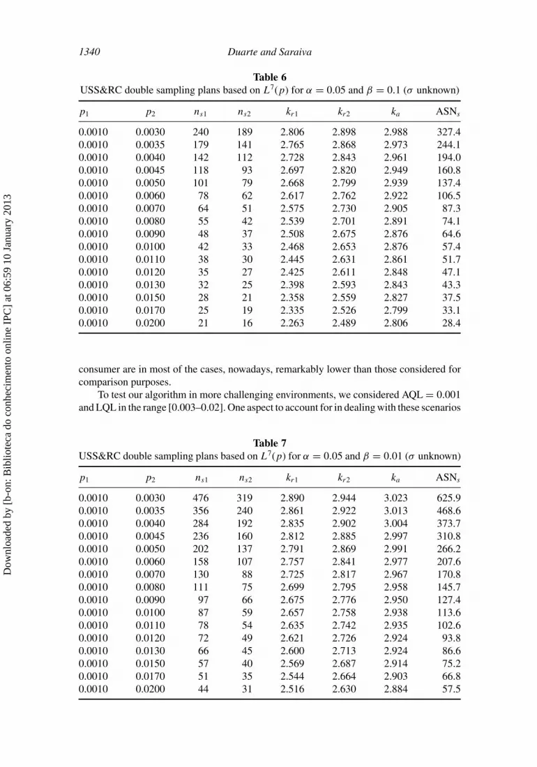
Table 6USS&RC double sampling plans based on L7(p) for α = 0.05 and β = 0.1 (σ unknown)

p1 p2 ns1 ns2 kr1 kr2 ka ASNs

0.0010 0.0030 240 189 2.806 2.898 2.988 327.40.0010 0.0035 179 141 2.765 2.868 2.973 244.10.0010 0.0040 142 112 2.728 2.843 2.961 194.00.0010 0.0045 118 93 2.697 2.820 2.949 160.80.0010 0.0050 101 79 2.668 2.799 2.939 137.40.0010 0.0060 78 62 2.617 2.762 2.922 106.50.0010 0.0070 64 51 2.575 2.730 2.905 87.30.0010 0.0080 55 42 2.539 2.701 2.891 74.10.0010 0.0090 48 37 2.508 2.675 2.876 64.60.0010 0.0100 42 33 2.468 2.653 2.876 57.40.0010 0.0110 38 30 2.445 2.631 2.861 51.70.0010 0.0120 35 27 2.425 2.611 2.848 47.10.0010 0.0130 32 25 2.398 2.593 2.843 43.30.0010 0.0150 28 21 2.358 2.559 2.827 37.50.0010 0.0170 25 19 2.335 2.526 2.799 33.10.0010 0.0200 21 16 2.263 2.489 2.806 28.4

consumer are in most of the cases, nowadays, remarkably lower than those considered forcomparison purposes.

To test our algorithm in more challenging environments, we considered AQL = 0.001and LQL in the range [0.003–0.02]. One aspect to account for in dealing with these scenarios

Table 7USS&RC double sampling plans based on L7(p) for α = 0.05 and β = 0.01 (σ unknown)

p1 p2 ns1 ns2 kr1 kr2 ka ASNs

0.0010 0.0030 476 319 2.890 2.944 3.023 625.90.0010 0.0035 356 240 2.861 2.922 3.013 468.60.0010 0.0040 284 192 2.835 2.902 3.004 373.70.0010 0.0045 236 160 2.812 2.885 2.997 310.80.0010 0.0050 202 137 2.791 2.869 2.991 266.20.0010 0.0060 158 107 2.757 2.841 2.977 207.60.0010 0.0070 130 88 2.725 2.817 2.967 170.80.0010 0.0080 111 75 2.699 2.795 2.958 145.70.0010 0.0090 97 66 2.675 2.776 2.950 127.40.0010 0.0100 87 59 2.657 2.758 2.938 113.60.0010 0.0110 78 54 2.635 2.742 2.935 102.60.0010 0.0120 72 49 2.621 2.726 2.924 93.80.0010 0.0130 66 45 2.600 2.713 2.924 86.60.0010 0.0150 57 40 2.569 2.687 2.914 75.20.0010 0.0170 51 35 2.544 2.664 2.903 66.80.0010 0.0200 44 31 2.516 2.630 2.884 57.5

Dow

nloa

ded

by [

b-on

: Bib

liote

ca d

o co

nhec

imen

to o

nlin

e IP

C]

at 0

6:59

10

Janu

ary

2013

Optimal Design of Acceptance Sampling Plans 1341

is that normal approximations may not work for extreme tail probabilities (Wallis, 1947).Furthermore, the solution would require OC curves with higher discriminating power (steep-ness). The results shown in Table 6 are in good agreement with those of Schilling (1982)and demonstrate that our tool is successful in dealing with processes in this range of qualityrequirements. Schilling and Johnson (1980) recommend employing very small values of βfor safety purposes. These scenarios are also increasingly demanding for AS plans designtools because they also require highly discriminating OC curves. To test our algorithm forlower values of errors of type II, we consider β = 0.01 and the same range of LQL andAQL values used in Table 6. The results shown in Table 7 extend the ability of the approachto cases with low values of consumer’s risk corresponding to inspection for safety purposes.

5. Conclusion

This article employs an optimization-based approach for designing AS plans by variablesfor controlling nonconforming proportions when σ is unknown. The approach is applied tosingle and double AS plans, and uses rigorous algorithmic strategies to compute noncentralStudent’s t-statistics. In the design of single AS plans, noncentral Student’s t-statisticis employed to determine the acceptance probability of the decision regarding the lotacceptance/rejection. Noncentral Student’s t-cdf is calculated through a series expansion. Asimilar approach is used to compute the OC curve representing the acceptance probabilityof the first stage of decision for double AS plans. The acceptance probability of the secondstage of decision in double AS plans required by the OC curve proposed by Krumbholzand Rohr (2006) is determined with Gaussian quadrature rules. AS plans based on rigorousnoncentral Student’s t-statistic are compared with plans derived assuming nonstandardnormal approximations and with other plans available in the literature.

Our mathematical programming problem formulation stands on the minimization ofthe ASN, subject to constraints in the OC curve controlled points, and enables to robustlyand accurately cope with the design of single and double AS plans. The relaxed formulationof the optimization problems is solved by employing NLP solvers. This procedure allowsone to systematically address any kind of AS plan, guaranteeing that globally optimalsolutions are obtained. Furthermore, the feasibility of the AS plans is assured by the solver.

The use of rigorous noncentral Student’s t-distribution calculation schemes revealedthat some of the plans proposed by Sommers (1981) are unfeasible, denoting consistentviolations of the constraint holding at LQL. AS plans based on normal distribution approx-imations were addressed, and two different assumptions were considered: (i) the statisticstested in both stages of decision follow the same normal distribution, and (ii) the statisticstested in each stage of decision follow different normal distribution approximations. Thedesigns obtained with the rigorous treatment of noncentral Student’s t-statistics are consis-tent with those produced employing normal distribution approximations. The approach wassuccessfully tested using a battery of scenarios available in the literature, outperforming theresults in some of the cases. To analyze its ability to cope with more challenging problemsdue to the requirement of higher discriminating power, it was also tested in environmentscharacterized by lower AQL and LQL values and different consumer’s risks, thus denotinglarge accuracy.

References

Abramowitz, M., Stegun, I. (1972). Handbook of Mathematical Functions. New York: DoverPulications.

Dow

nloa

ded

by [

b-on

: Bib

liote

ca d

o co

nhec

imen

to o

nlin

e IP

C]

at 0

6:59

10

Janu

ary

2013

1342 Duarte and Saraiva

Balamurali, S., Jun, C.-H. (2007). Multiple dependent state sampling plans for lot acceptance basedon measurement data. European Journal Operational Research 180:1221–1230.

Bowker, A. H., Goode, H. P. (1952). Sampling Inspection by Variables. New York: McGraw-Hill.Drud, A. (1985). CONOPT: A GRG code for large sparse dynamic nonlinear optimization problems.

Mathematical Programming 31:153–191.Duarte, B., Saraiva, P. (2010). An optimization-based framework for designing acceptance sampling

plans by variables for nonconforming proportions. International Journal Quality and ReliabilityEngineering 27:794–814.

Duncan, A. (1974). Quality Control and Industrial Statistics. 4th ed. Homewood, IL: Richard D.Irwin.

Evans, J. R. (2005). Total Quality – Management, Organizations and Strategy. 4th ed. Toronto,Canada: Thomson.

Feldmann, B., Krumbholz, W. (2002). ASN-Minimax double sampling plans for variables. StatisticalPapers 43:361–377.

Gelbard, F., Seinfeld, J. (1978). Numerical solution of the dynamic equation for particulate systems.Journal of Computational Physics 28:357–375.

Guenther, W. (1978). Evaluation of the probabilities for the noncentral distributions and the differenceof two t-variables with a desk calculator. Journal of Statistical Computation and Simulation6:199–206.

Hamaker, H. C. (1979). Acceptance sampling for percent defective by variables and by attributes.Journal of Quality Technology 11:139–148.

Hilbert, M. (2005). Zweifache ASN-Minimax-Variablenprufplane fur normalverteiltes Merkmal beiunbekannten Parametern. Ph.D. thesis. Hamburg: Universitat der Bundeswehr Hamburg.

Krumbholz, W., Rohr, A. (2006). The operating characteristic of double sampling plans by variableswhen the standard deviation is unknown. Allgemeines Statistisches Archiv 90:233–251.

Lenth, R. (1989). Algorithm AS 243: cumulative distribution function of the non-central t distribution.Applied Statistics 38:185–189.

Mitra, A. (1998). Fundamentals of Quality Control and Improvement. 2nd ed. Upper Saddle River,NJ: Prentice-Hall.

Schilling, E. G. (1982). Acceptance Sampling in Quality Control. New York: Marcel Dekker.Schilling, E. G., Johnson, L. (1980). Tables for the construction of matched single, double, and

multiple sampling plans with application to MIL-STD-105D. Journal of Quality Technology12:220–229.

Seidel, W. (1997). Is sampling by variables worse than sampling by attributes? A decision theoreticanalysis and a new mixed strategy for inspecting individual lots. Sankhya B 59:6–107.

Sommers, D. J. (1981). Two-point double variables sampling plans. Journal of Quality Technology13:5–30.

Wallis, W. A. (1947). Techniques of Statistical Analysis. New York: McGraw-Hill.

Dow

nloa

ded

by [

b-on

: Bib

liote

ca d

o co

nhec

imen

to o

nlin

e IP

C]

at 0

6:59

10

Janu

ary

2013