optimal bank capital*

Optimal Bank Capital

David MilesMonetary Policy Committee

The Bank of EnglandMarch 2011

5

10

15

20

25

30

35

40

-3%

-2%

-1%

0%

1%

2%

3%

4%

5%

1880 1900 1920 1940 1960 1980 2000

Real GDP growth 10y-MA

Leverage (rhs)(a)

(c)(b)

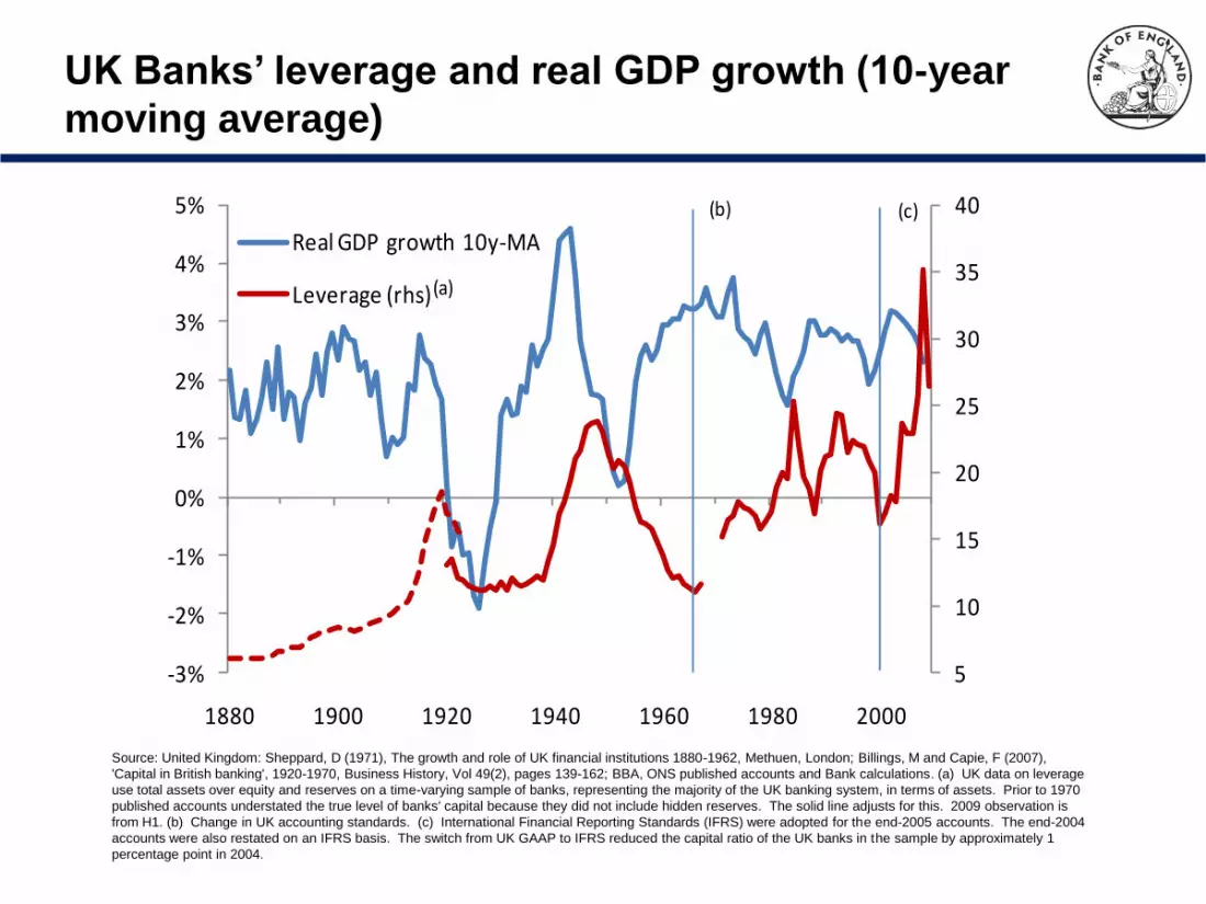
UK Banks’ leverage and real GDP growth (10-year

moving average)

Source: United Kingdom: Sheppard, D (1971), The growth and role of UK financial institutions 1880-1962, Methuen, London; Billings, M and Capie, F (2007),

'Capital in British banking', 1920-1970, Business History, Vol 49(2), pages 139-162; BBA, ONS published accounts and Bank calculations. (a) UK data on leverage

use total assets over equity and reserves on a time-varying sample of banks, representing the majority of the UK banking system, in terms of assets. Prior to 1970

published accounts understated the true level of banks' capital because they did not include hidden reserves. The solid line adjusts for this. 2009 observation is

from H1. (b) Change in UK accounting standards. (c) International Financial Reporting Standards (IFRS) were adopted for the end-2005 accounts. The end-2004

accounts were also restated on an IFRS basis. The switch from UK GAAP to IFRS reduced the capital ratio of the UK banks in the sample by approximately 1

percentage point in 2004.

0

2

4

6

8

10

12

14

16

18

20

0

1

2

3

4

5

6

1920 1930 1940 1950 1960 1970 1980

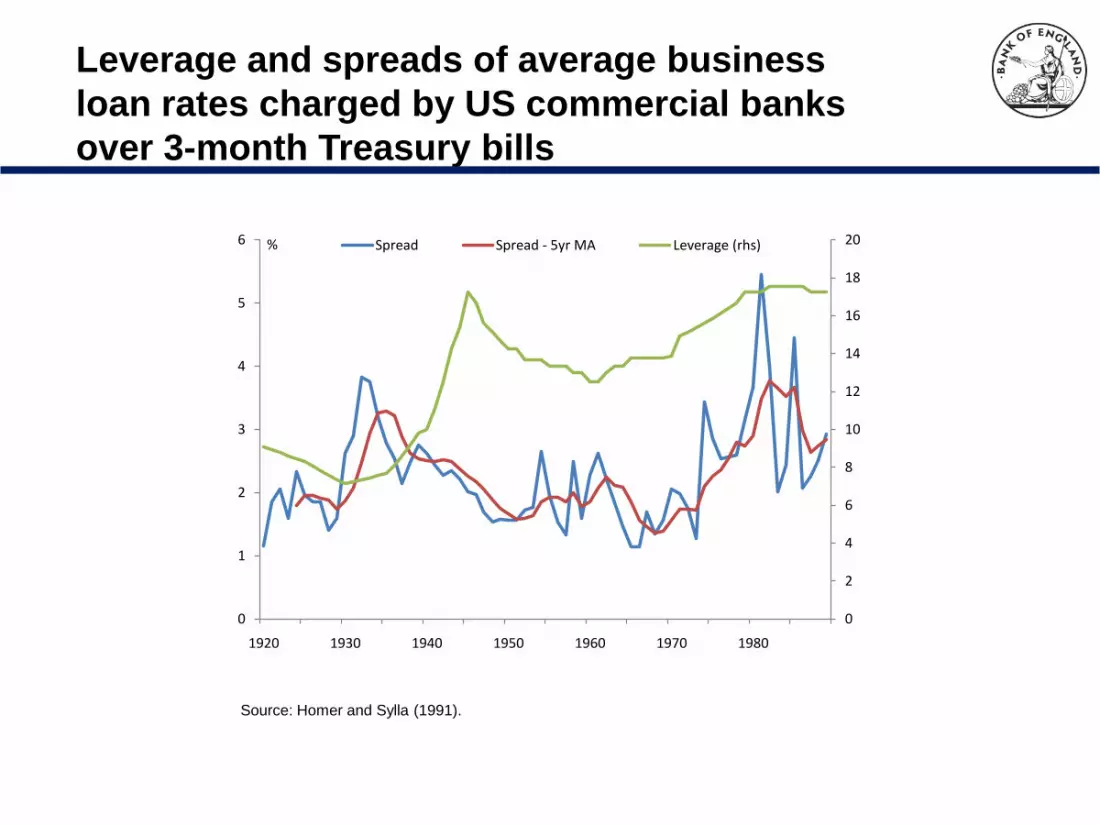
Spread Spread - 5yr MA Leverage (rhs)%

Leverage and spreads of average business

loan rates charged by US commercial banks

over 3-month Treasury bills

Source: Homer and Sylla (1991).

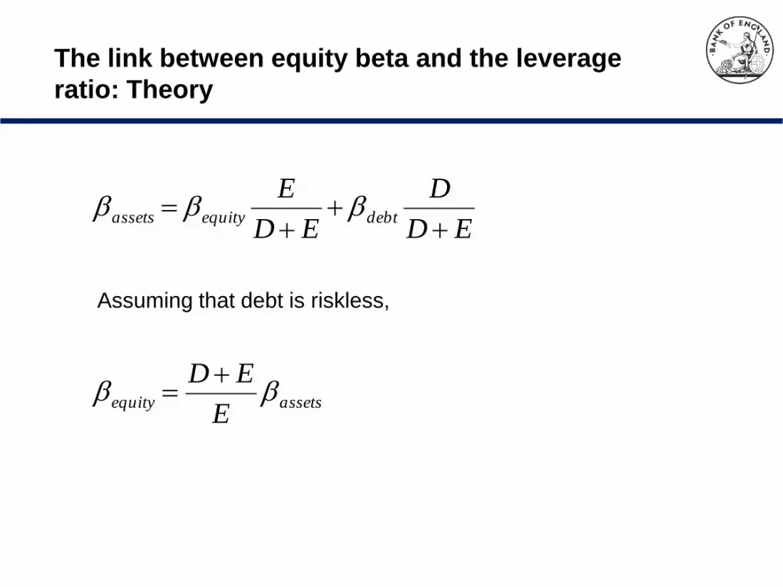
Assuming that debt is riskless,

The link between equity beta and the leverage

ratio: Theory

ED

D

ED

Edebtequityassets

assetsequityE

ED

Average equity beta across major UK

banks, 1997-2010

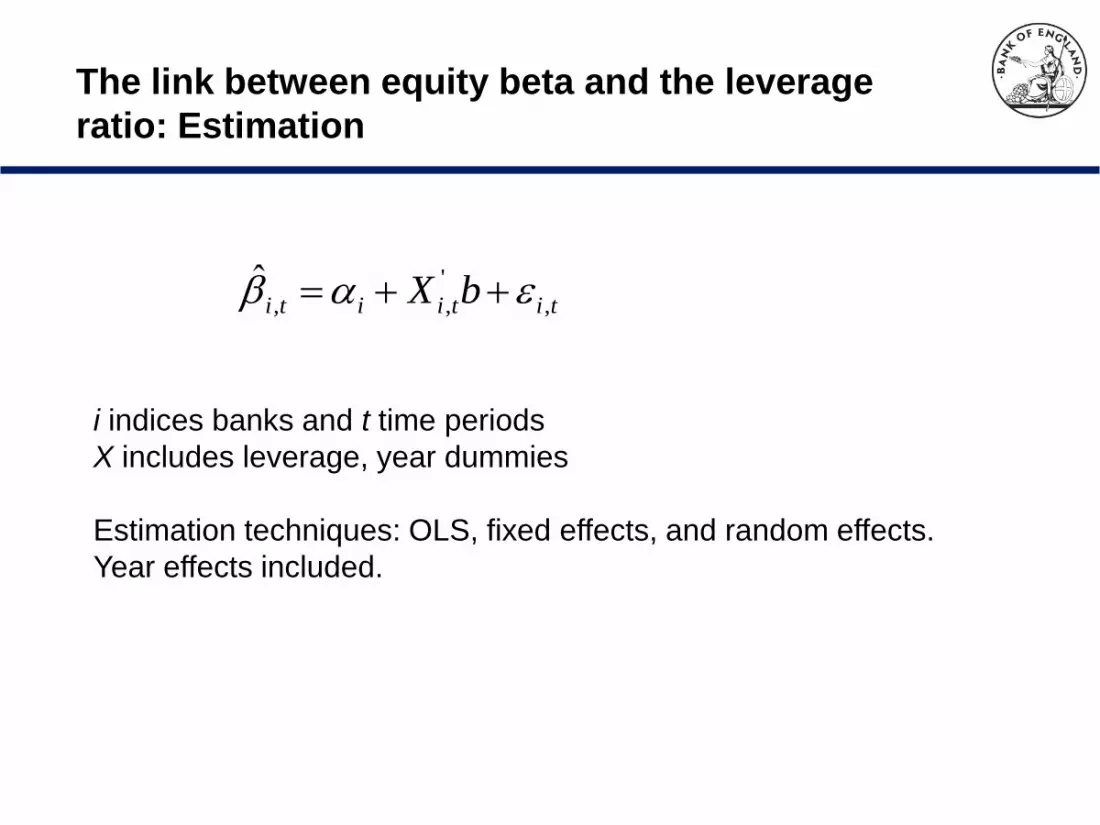
i indices banks and t time periods

X includes leverage, year dummies

Estimation techniques: OLS, fixed effects, and random effects.

Year effects included.

The link between equity beta and the leverage

ratio: Estimation

titiiti bX ,

'

,,ˆ

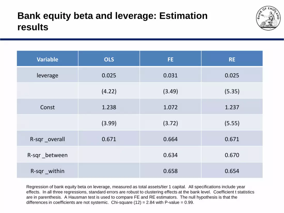
Bank equity beta and leverage: Estimation

results

Variable OLS FE RE

leverage 0.025 0.031 0.025

(4.22) (3.49) (5.35)

Const 1.238 1.072 1.237

(3.99) (3.72) (5.55)

R-sqr _overall 0.671 0.664 0.671

R-sqr _between 0.634 0.670

R-sqr _within 0.658 0.654

Regression of bank equity beta on leverage, measured as total assets/tier 1 capital. All specifications include year

effects. In all three regressions, standard errors are robust to clustering effects at the bank level. Coefficient t statistics

are in parenthesis. A Hausman test is used to compare FE and RE estimators. The null hypothesis is that the

differences in coefficients are not systemic. Chi-square (12) = 2.84 with P-value = 0.99.

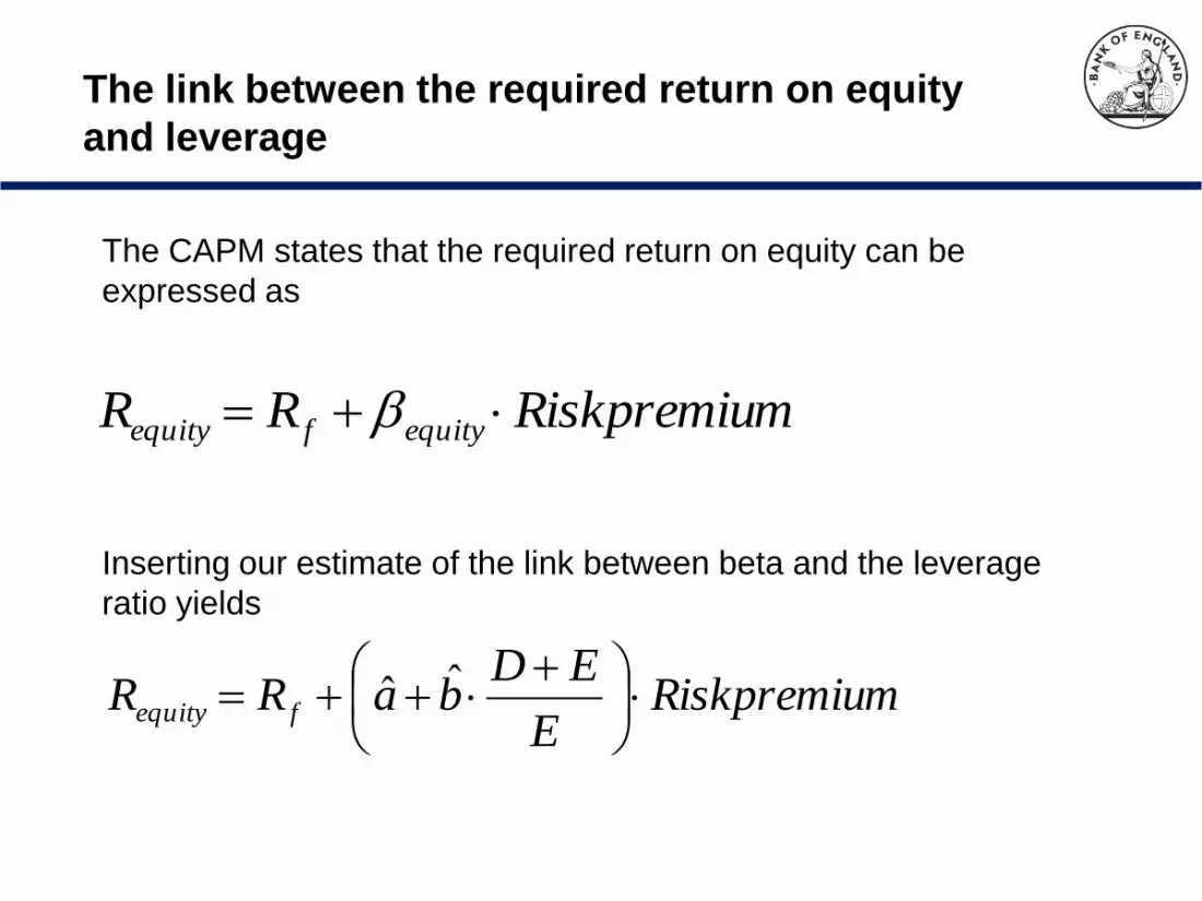
The link between the required return on equity

and leverage

mRiskpremiuRR equityfequity

The CAPM states that the required return on equity can be

expressed as

Inserting our estimate of the link between beta and the leverage

ratio yields

mRiskpremiuE

EDbaRR fequity

ˆˆ

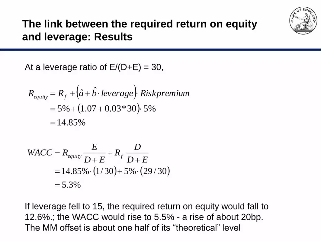
The link between the required return on equity

and leverage: Results

At a leverage ratio of E/(D+E) = 30,

%85.14

%530*03.007.1%5

ˆˆ

mRiskpremiuleveragebaRR fequity

%3.5

30/29%530/1%85.14

ED

DR

ED

ERWACC fequity

If leverage fell to 15, the required return on equity would fall to

12.6%.; the WACC would rise to 5.5% - a rise of about 20bp.

The MM offset is about one half of its “theoretical” level

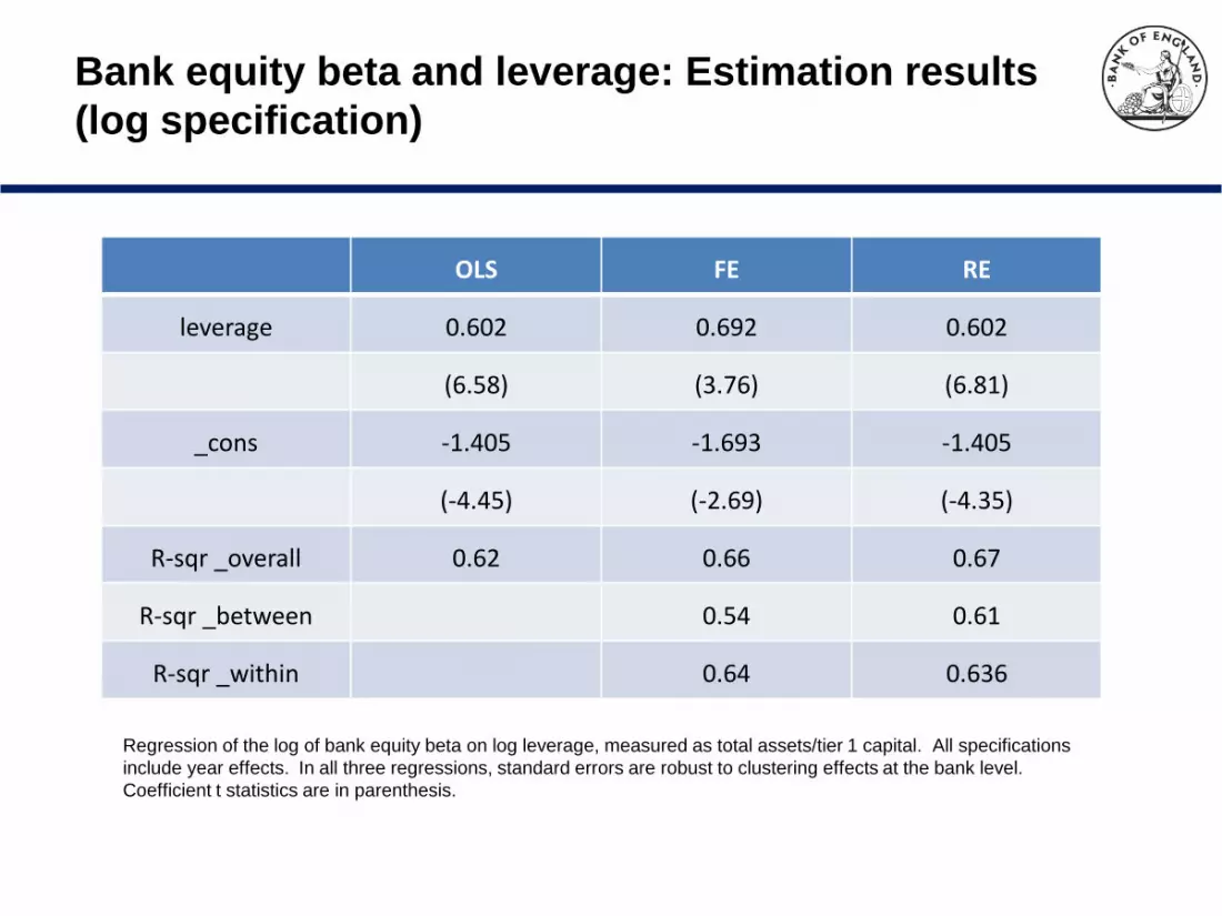
OLS FE RE

leverage 0.602 0.692 0.602

(6.58) (3.76) (6.81)

_cons -1.405 -1.693 -1.405

(-4.45) (-2.69) (-4.35)

R-sqr _overall 0.62 0.66 0.67



Bank equity beta and leverage: Estimation results

(log specification)

Regression of the log of bank equity beta on log leverage, measured as total assets/tier 1 capital. All specifications

include year effects. In all three regressions, standard errors are robust to clustering effects at the bank level.

Coefficient t statistics are in parenthesis.

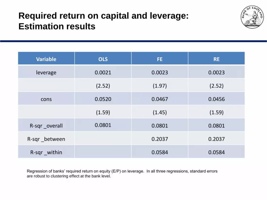
Variable OLS FE RE

leverage 0.0021 0.0023 0.0023

(2.52) (1.97) (2.52)

cons 0.0520 0.0467 0.0456

(1.59) (1.45) (1.59)

R-sqr _overall 0.0801 0.0801 0.0801

R-sqr _between 0.2037 0.2037

R-sqr _within 0.0584 0.0584

Required return on capital and leverage:

Estimation results

Regression of banks’ required return on equity (E/P) on leverage. In all three regressions, standard errors

are robust to clustering effect at the bank level.

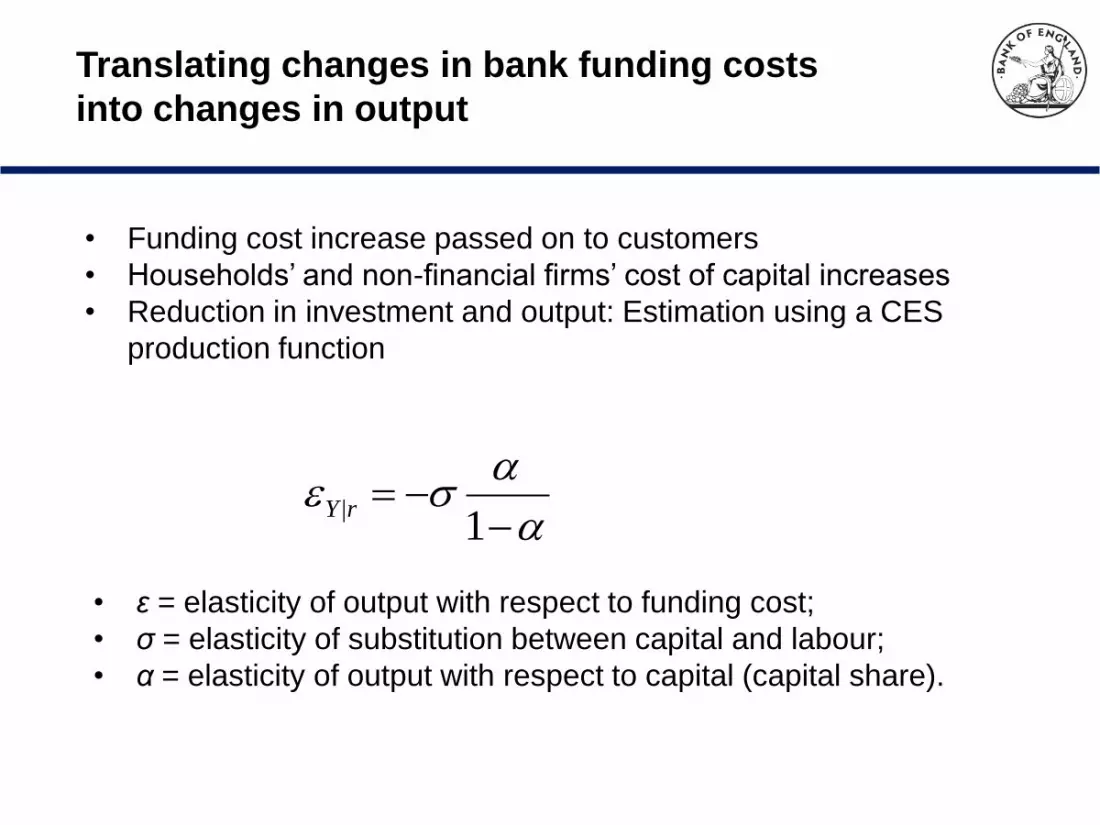
Translating changes in bank funding costs

into changes in output

• Funding cost increase passed on to customers

• Households’ and non-financial firms’ cost of capital increases

• Reduction in investment and output: Estimation using a CES

production function

1|rY

• ε = elasticity of output with respect to funding cost;

• σ = elasticity of substitution between capital and labour;

• α = elasticity of output with respect to capital (capital share).

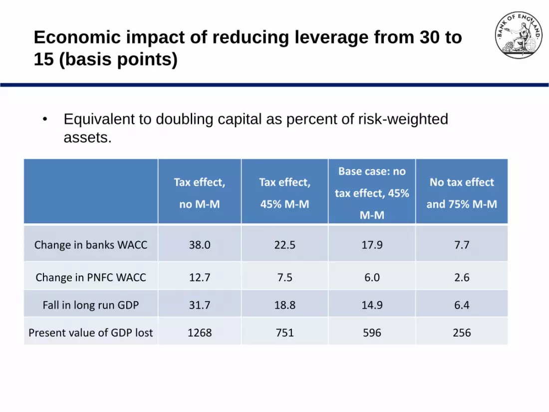
Tax effect,

no M-M

Tax effect,

45% M-M

Base case: no

tax effect, 45%

M-M

No tax effect

and 75% M-M

Change in banks WACC 38.0 22.5 17.9 7.7

Change in PNFC WACC 12.7 7.5 6.0 2.6

Fall in long run GDP 31.7 18.8 14.9 6.4

Present value of GDP lost 1268 751 596 256

Economic impact of reducing leverage from 30 to

15 (basis points)

• Equivalent to doubling capital as percent of risk-weighted

assets.

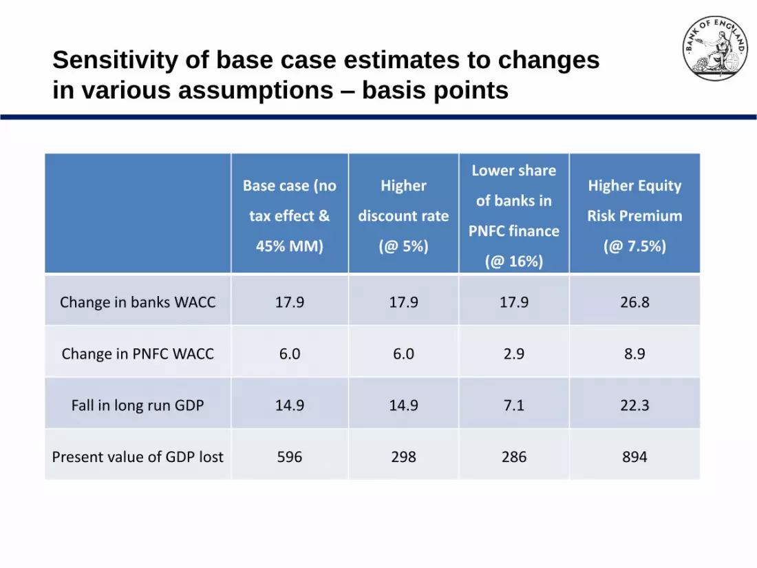
Base case (no

tax effect &

45% MM)

Higher

discount rate

(@ 5%)

Lower share

of banks in

PNFC finance

(@ 16%)

Higher Equity

Risk Premium

(@ 7.5%)

Change in banks WACC 17.9 17.9 17.9 26.8

Change in PNFC WACC 6.0 6.0 2.9 8.9

Fall in long run GDP 14.9 14.9 7.1 22.3

Present value of GDP lost 596 298 286 894

Sensitivity of base case estimates to changes

in various assumptions – basis points

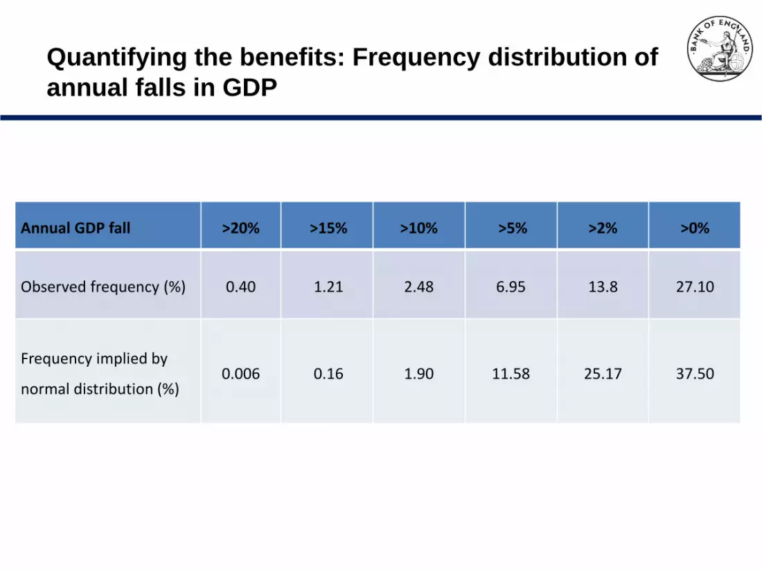
Quantifying the benefits: Frequency distribution of

annual falls in GDP

Annual GDP fall >20% >15% >10% >5% >2% >0%

Observed frequency (%) 0.40 1.21 2.48 6.95 13.8 27.10

Frequency implied by

normal distribution (%) 0.006 0.16 1.90 11.58 25.17 37.50

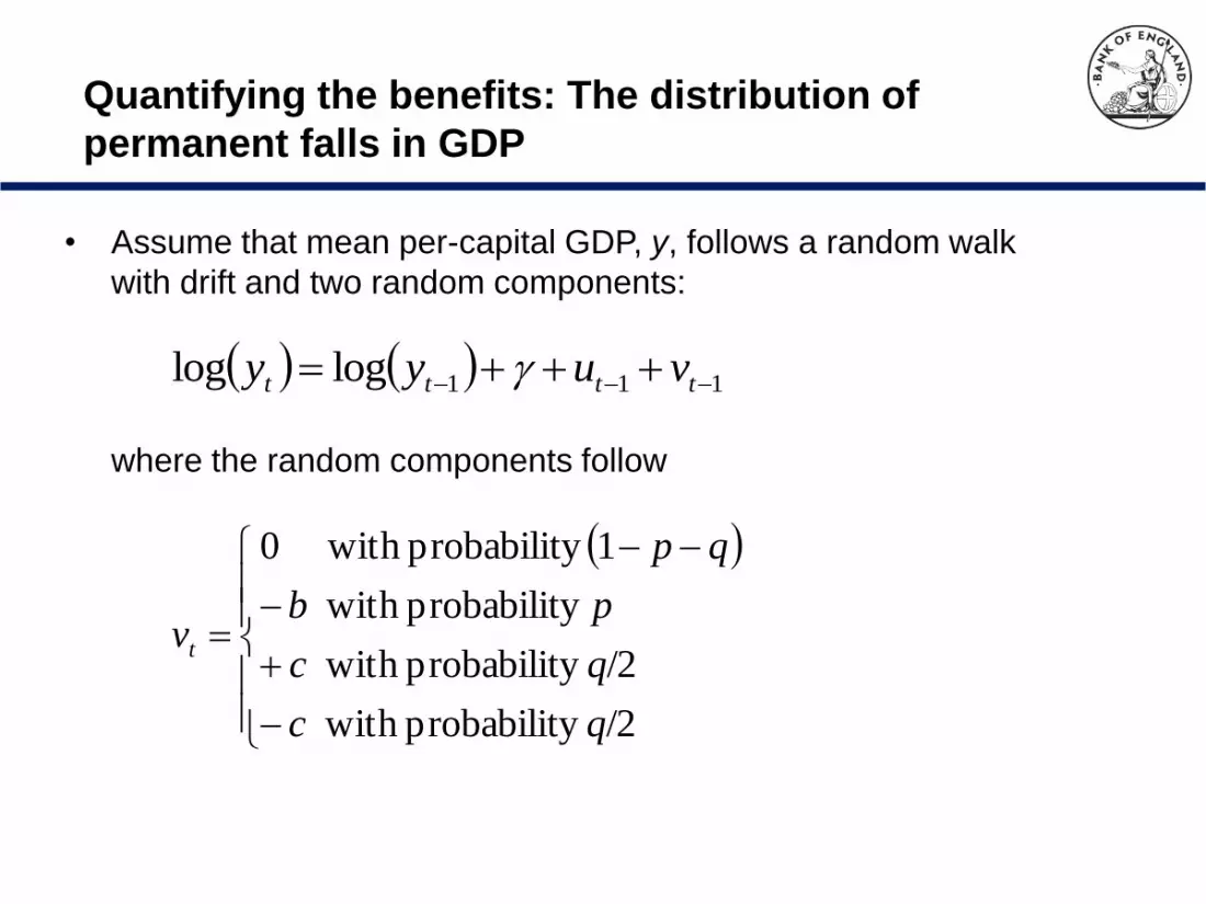
Quantifying the benefits: The distribution of

permanent falls in GDP

• Assume that mean per-capital GDP, y, follows a random walk

with drift and two random components:

111loglog tttt vuyy

where the random components follow

/2y probabilit with

/2y probabilit with

y probabilit with

1y probabilit with 0

qc

qc

pb

qp

vt

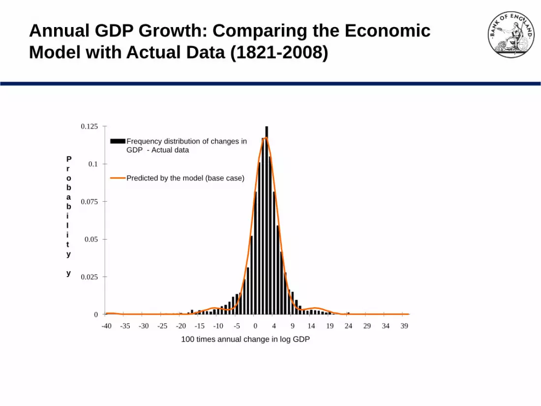
0

0.025

0.05

0.075

0.1

0.125

-40 -35 -30 -25 -20 -15 -10 -5 0 4 9 14 19 24 29 34 39

Frequency distribution of changes in GDP - Actual data

Predicted by the model (base case)

P

r

o

b

a

b

i

I

i

t

y

y

100 times annual change in log GDP

Annual GDP Growth: Comparing the Economic

Model with Actual Data (1821-2008)

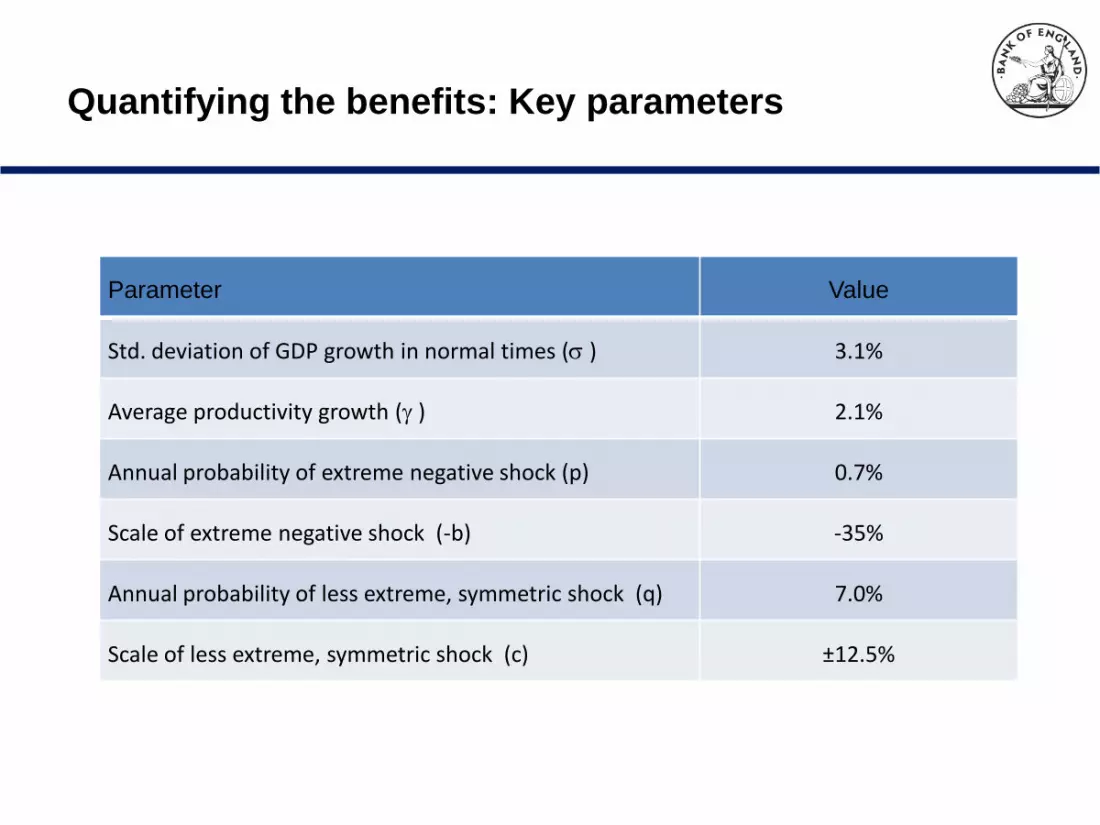
Parameter Value

Std. deviation of GDP growth in normal times ( ) 3.1%

Average productivity growth ( ) 2.1%

Annual probability of extreme negative shock (p) 0.7%

Scale of extreme negative shock (-b) -35%

Annual probability of less extreme, symmetric shock (q) 7.0%

Scale of less extreme, symmetric shock (c) ±12.5%

Quantifying the benefits: Key parameters

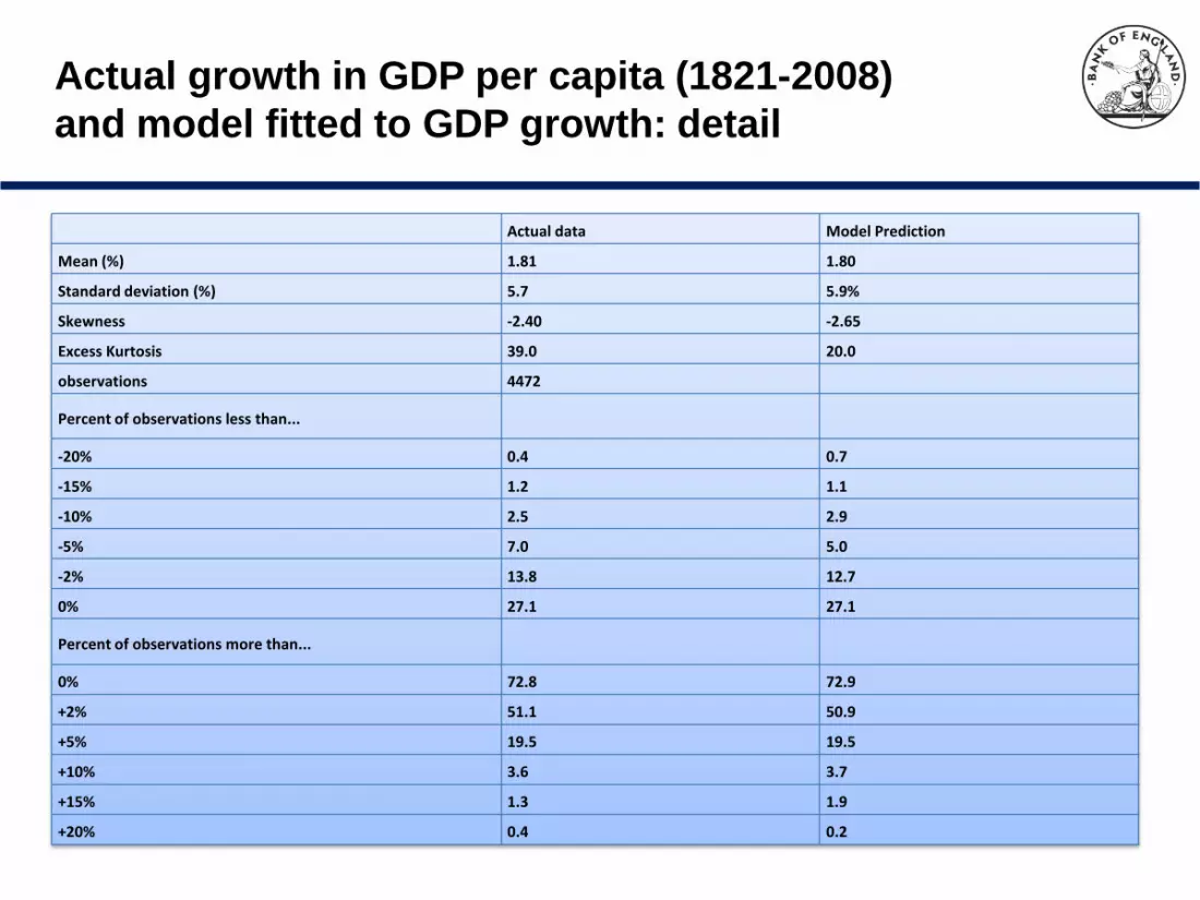
Actual data Model Prediction

Mean (%) 1.81 1.80

Standard deviation (%) 5.7 5.9%

Skewness -2.40 -2.65

Excess Kurtosis 39.0 20.0

observations 4472

Percent of observations less than...

-20% 0.4 0.7

-15% 1.2 1.1

-10% 2.5 2.9

-5% 7.0 5.0

-2% 13.8 12.7

0% 27.1 27.1

Percent of observations more than...

0% 72.8 72.9

+2% 51.1 50.9

+5% 19.5 19.5

+10% 3.6 3.7

+15% 1.3 1.9

+20% 0.4 0.2

Actual growth in GDP per capita (1821-2008)

and model fitted to GDP growth: detail

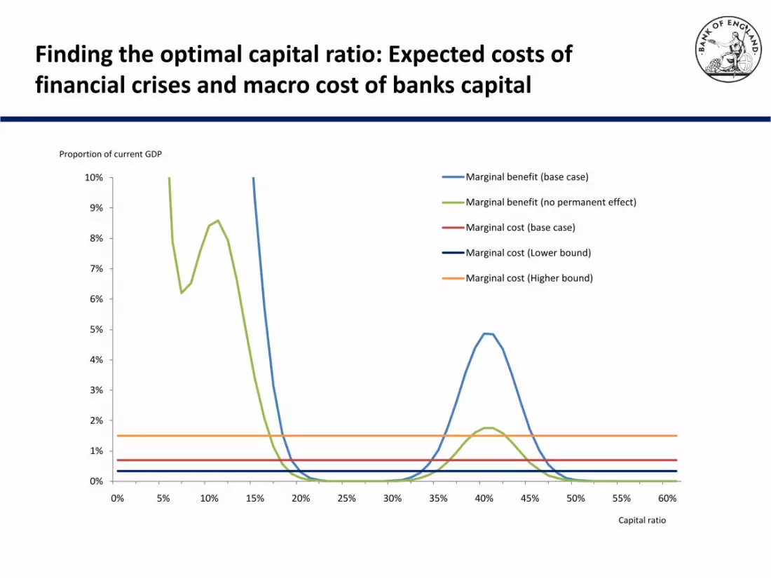
0%

1%

2%

3%

4%

5%

6%

7%

8%

9%

10%

0% 5% 10% 15% 20% 25% 30% 35% 40% 45% 50% 55% 60%

Marginal benefit (base case)

Marginal benefit (no permanent effect)

Marginal cost (base case)

Marginal cost (Lower bound)

Marginal cost (Higher bound)

Capital ratio

Proportion of current GDP

Finding the optimal capital ratio: Expected costs of financial crises and macro cost of banks capital

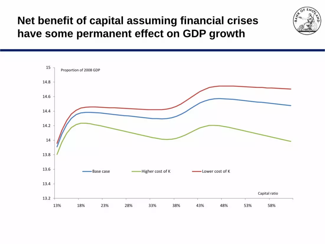
13.2

13.4

13.6

13.8

14

14.2

14.4

14.6

14.8

15

13% 18% 23% 28% 33% 38% 43% 48% 53% 58%

Base case Higher cost of K Lower cost of K

Proportion of 2008 GDP

Capital ratio

Net benefit of capital assuming financial crises

have some permanent effect on GDP growth

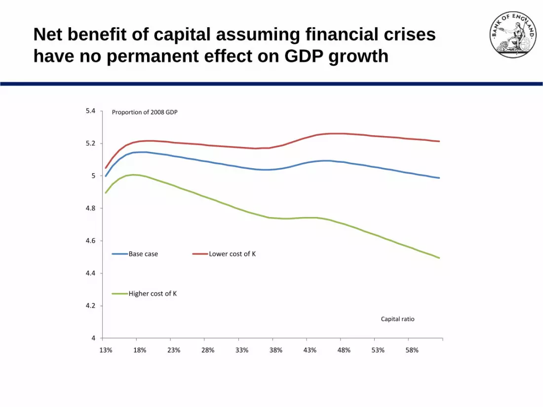
4

4.2

4.4

4.6

4.8

5

5.2

5.4

13% 18% 23% 28% 33% 38% 43% 48% 53% 58%

Base case Lower cost of K

Higher cost of K

Proportion of 2008 GDP

Capital ratio

Net benefit of capital assuming financial crises

have no permanent effect on GDP growth

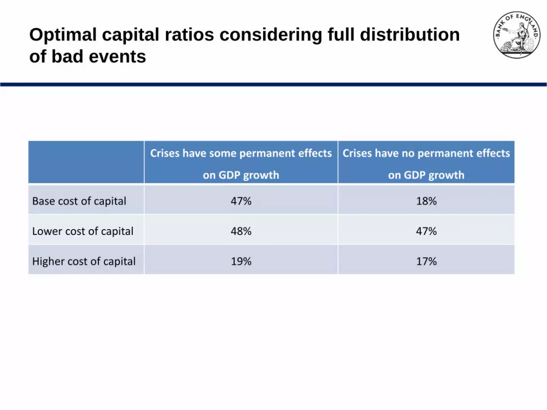
Optimal capital ratios considering full distribution

of bad events

Crises have some permanent effects

on GDP growth

Crises have no permanent effects

on GDP growth

Base cost of capital 47% 18%

Lower cost of capital 48% 47%

Higher cost of capital 19% 17%

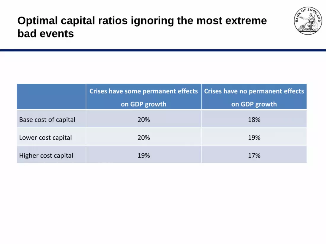
Optimal capital ratios ignoring the most extreme

bad events

Crises have some permanent effects

on GDP growth

Crises have no permanent effects

on GDP growth

Base cost of capital 20% 18%

Lower cost capital 20% 19%

Higher cost capital 19% 17%

Backup slides

• Detailed estimation results

• Actual growth in GDP per capita (1821-2008) and model fitted to GDP growth

Bank equity beta and leverage: Estimation

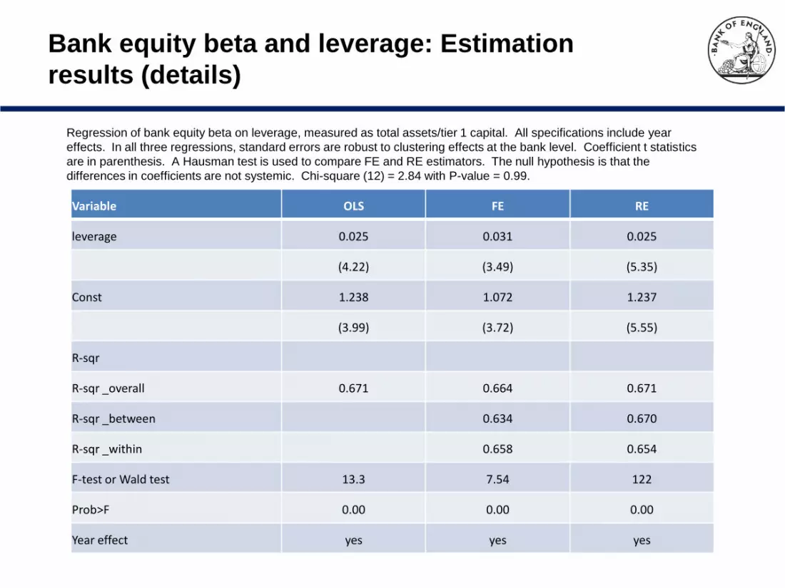
results (details)

Variable OLS FE RE

leverage 0.025 0.031 0.025

(4.22) (3.49) (5.35)

Const 1.238 1.072 1.237

(3.99) (3.72) (5.55)

R-sqr

R-sqr _overall 0.671 0.664 0.671



F-test or Wald test 13.3 7.54 122

Prob>F 0.00 0.00 0.00

Year effect yes yes yes

Regression of bank equity beta on leverage, measured as total assets/tier 1 capital. All specifications include year

effects. In all three regressions, standard errors are robust to clustering effects at the bank level. Coefficient t statistics

are in parenthesis. A Hausman test is used to compare FE and RE estimators. The null hypothesis is that the

differences in coefficients are not systemic. Chi-square (12) = 2.84 with P-value = 0.99.

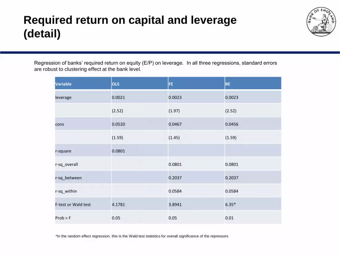
Variable OLS FE RE

leverage 0.0021 0.0023 0.0023

(2.52) (1.97) (2.52)

cons 0.0520 0.0467 0.0456

(1.59) (1.45) (1.59)

r-square 0.0801

r-sq_overall 0.0801 0.0801

r-sq_between 0.2037 0.2037

r-sq_within 0.0584 0.0584

F-test or Wald test 4.1781 3.8941 6.35*

Prob > F 0.05 0.05 0.01

Required return on capital and leverage

(detail)

*In the random effect regression, this is the Wald test statistics for overall significance of the repressors

Regression of banks’ required return on equity (E/P) on leverage. In all three regressions, standard errors

are robust to clustering effect at the bank level.

optimal bank capital*

Documents