Optical conductivity of the Holstein polaron

Glen L. Goodvin1, Andrey S. Mishchenko2,3 and Mona Berciu1

1Department of Physics & Astronomy, University of British Columbia, Vancouver, BC, Canada, V6T 1Z12Cross-Correlated Materials Research Group (CMRG), ASI, RIKEN, Wako 351-0198, Japan

3Russian Research Centre “Kurchatov Institute”, 123182 Moscow, Russia(Dated: September 20, 2011)

The Momentum Average approximation is used to derive a new kind of non-perturbational ana-lytical expression for the optical conductivity (OC) of a Holstein polaron at zero temperature. Thisprovides insight into the shape of the OC, by linking it to the structure of the polaron’s phononcloud. Our method works in any dimension, properly enforces selection rules, can be systematicallyimproved, and also generalizes to momentum-dependent couplings. Its accuracy is demonstrated bya comparison with the first detailed set of three-dimensional numerical OC results, obtained usingthe approximation-free diagrammatic Monte Carlo method.

PACS numbers: 71.38.-k, 72.10.Di, 63.20.kd

Although the study of polarons is one of the older prob-lems in solid state physics [1], a full understanding oftheir properties is still missing. This is especially true forthe excited states which influence response functions likethe optical conductivity (OC). OC measurements haverevealed the role of the electron-phonon (el-ph) couplingin many materials, e.g., cuprates [2] and manganites [3].In particular, the shape of the OC curve is important, asit signifies large versus small polaron behavior [4].

The OC of polarons has been studied numerically us-ing exact diagonalization in 1D [5] and for small clus-ters in higher dimension (here, finite size effects can bean issue) [6]. There are also some diagrammatic MonteCarlo (DMC) results for the 3D Frohlich and 2D Holsteinmodels [7]. DMC gives approximation-free results in thethermodynamic limit, but it requires significant compu-tational effort; this is why there are very few DMC OCsets available in the literature. The conceptual problemassociated with all numerical methods, however, is thatthey do not provide much insight for understanding theshape of the OC and its relation to the properties of thepolaron. Analytical expressions are needed for this, butmost prior work was limited to perturbational regimes [8].The one exception is work based on the dynamical mean-field theory (DMFT) [9], which however ignores currentvertex corrections. The consequences are discussed be-low; here we state only that a complete understanding ofthe shape of the OC is still not achieved using it.

It is, then, hard to overemphasize the need for an accu-rate analytical expression establishing a nonperturbativestructure of the OC. In this Letter we obtain such anexpression using a generalization of the Momentum Av-erage (MA) approximation. MA was developed for thesingle-particle Green’s function of the Holstein polaron[10] and then extended to more complex models [11], in-cluding disorder [12]. It is non-perturbational since itsums all self-energy diagrams, up to exponentially smallterms which are discarded. MA becomes exact in vari-ous asymptotic limits, satisfies multiple spectral weight

sum rules, is quantitatively accurate in any dimension,at all energies for all parameters except in the extremeadiabatic limit, and can be systematically improved [10].

Here we show how to use MA to calculate two-particleGreen’s functions, needed in response functions like theOC. Besides efficient yet accurate results at any cou-pling, this finally provides the explanation for the physi-cal meaning of the shape of the OC. Moreover, this MA-based approach generalizes to OC calculations for modelswith momentum-dependent el-ph coupling [11].

We use the Holstein model [13] as a specific examplesince some numerical data is available for comparison:

H =∑k

(εkc†kck + Ωb†kbk

)+

g√N

∑k,q

c†k−qck(b†q + b−q

).

Here, c†k and b†k are electron and boson creation operatorsfor a state of momentum k (the electron’s spin is trivialand we suppress its index). The free electron dispersion

εk = −2t∑di=1 cos(kia) is for nearest-neighbor hopping

on a d-dimensional hypercubic lattice of constant a, andthe Einstein optical phonons have energy Ω. The lastterm describes the local el-ph coupling g

∑i c†i ci(b

†i + bi),

written in k-space. All sums over momenta are over theBrillouin zone and we take the total number N of sitesto infinity. We set h = 1 and a = 1 throughout.

For the case we study here, i.e. a single polaron atT = 0, the optical conductivity is given by the Kuboformula [14]:

σ(ω) =1

ωV

∫ ∞0

dteiωt〈ψ0|[j†(t), j(0)]|ψ0〉, (1)

with V the volume, |ψ0〉 the polaron ground state (GS),and the charge current operator j = 2et

∑q sin qc†qcq is

in the Heisenberg picture. Here, e is the electron chargeand q the component of q parallel to the electric field.

Our main result is that the optical absorption equals:

Re [σMA(i)(ω)] =4πe2t2

ω

∑n≥1

P (i)n f (i)

n (ω). (2)

arX

iv:1

109.

3749

v1 [

cond

-mat

.str

-el]

17

Sep

2011

2

Here i ≥ 0 is the level of MA(i) approximation, denotingan increasing complexity of the variational description ofthe eigenstates [10]. However, the physical meaning is the

same: P(i)n is the GS probability to have n phonons at the

electron site, while f(i)n (ω) are spectral functions describ-

ing the electron’s optical absorption in this n-phonon en-vironment. Eq. (2) shows the direct link between theOC and the structure of the polaron’s phonon cloud.

Further discussion is provided below. First, we deriveEq. (2) so that the meaning of various quantities becomesclear. Expanding the commutator and doing the integralin Eq. (1), we find σ(ω) = σ+(ω) + (σ+(−ω))

∗, with:

σ+(ω) =i

ωV〈ψ0|jG(ω + E0)j|ψ0〉, (3)

where G(ω) = [ω+ iη−H]−1 with η → 0+, and E0 is thepolaron GS energy. The usual route is to use a Lehmannrepresentation, leading to the well-known formula:

σ(ω) =π

ωV

∑n

|〈ψ0|j|ψn〉|2δ(ω + E0 − En) (4)

in terms of excited polaron eigenstates |ψn〉, En. Instead,we use twice the resolution of identity to rewrite:

σ+(ω) =i(2et)2

ωV

∑q,Q

sin q sinQ∑α,β

〈ψ0|c†q|α〉

× Fαβ(q,Q, ω + E0)〈β|cQ|ψ0〉, (5)

where Fαβ(q,Q, ω) = 〈α|cqG(ω)c†Q|β〉. Since |ψ0〉 isthe polaron GS, |α〉 and |β〉 are phonon-only states.Moreover, because of invariance to translations, their mo-mentum is −q, respectively −Q. Eq. (5) is exact.

Consider now these matrix elements within MA(0),whose variational meaning is to expand polaron eigen-states in the basis c†i (b

†j)n|0〉, (∀)i, j, n [10, 16]. Then,

|α〉 → | − q, n〉 = 1√N

∑i e−iq·Ri(b†i )

n|0〉, since only such

states will have finite overlaps in Eq. (5). The sums overα, β are now sums over phonons numbers n,m ≥ 1. Notethat n,m = 0 do not contribute to the regular part ofσ(ω) since | − q, 0〉 ∼ δq,0|0〉, and sin q · δq,0 → 0. Theydo contribute to the Drude peak, Dδ(ω).

The calculation of the single electron Green’s func-tions Fnm(q,Q, ω) = 〈−q, n|cqG(ω)c†Q| − Q,m〉 and of

the residues 〈ψ0|c†q| − q, n〉 is now carried out. Detailsare provided in the supplementary material at the endof this article. Here, we note that because of the oddsin q, sinQ terms, only the part of Fnm(q,Q, ω) propor-tional to δq,Qδn,m has non-vanishing contribution to Eq.(5), explaining the single sum over n ≥ 1 in Eq. (2). Fi-nally, the overlap |〈ψ0|c†q| − q, n〉|2 is linked to the prob-ability Pn to have n phonons at the electron site in thepolaron GS [17]. The Pn expressions are listed in the sup-plementary material. Altogether, we obtain the result of

0 1 2 3 4n

0

0.2

0.4

0.6

0.8

1

Pn

λ=0.003λ=0.5λ=1.0

0 5 10 15 20 25 30n

0

0.03

0.06

0.09

0.12

λ=1.04λ=1.25λ=1.25, LF

3D: Ω/t=0.5

(a) (b)

_

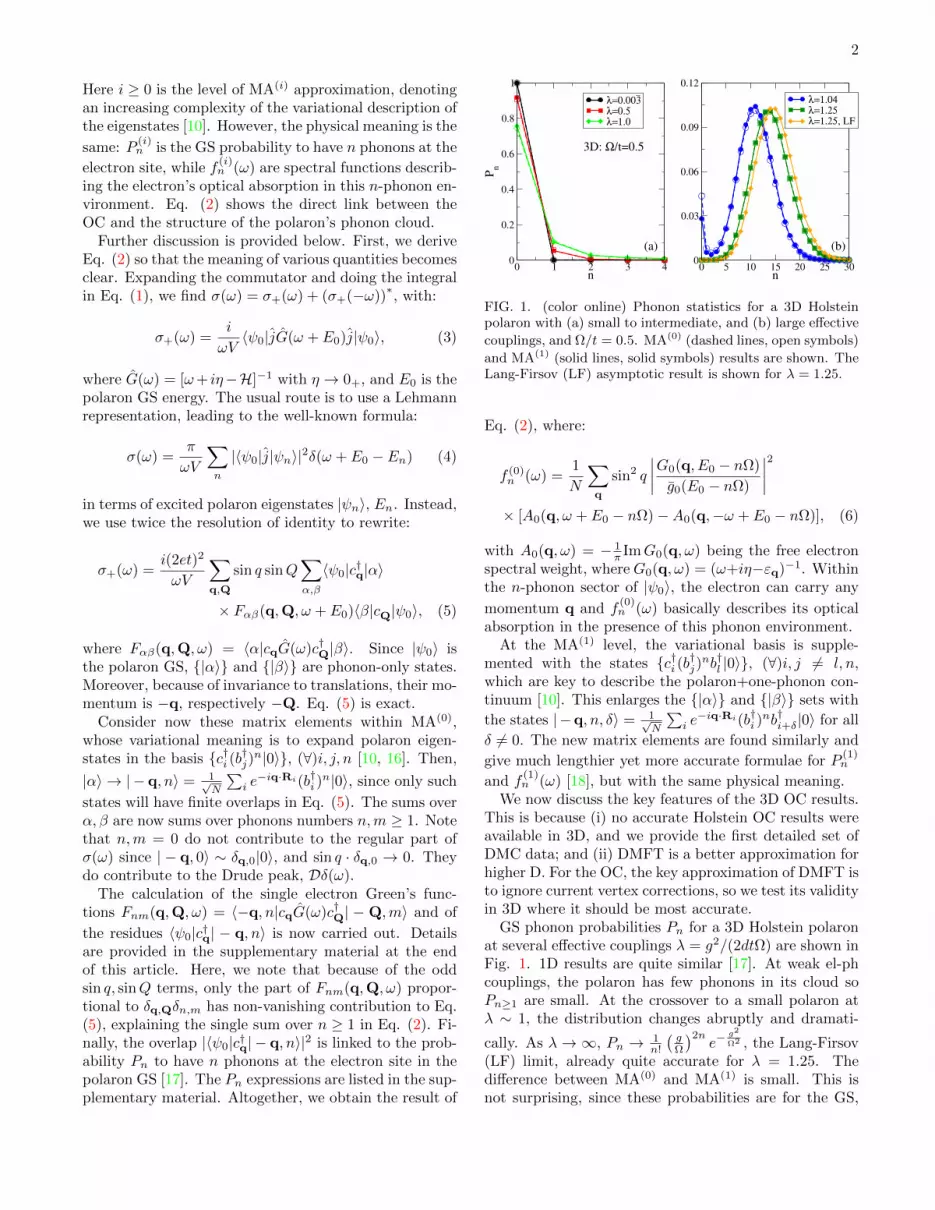
FIG. 1. (color online) Phonon statistics for a 3D Holsteinpolaron with (a) small to intermediate, and (b) large effective

couplings, and Ω/t = 0.5. MA(0) (dashed lines, open symbols)

and MA(1) (solid lines, solid symbols) results are shown. TheLang-Firsov (LF) asymptotic result is shown for λ = 1.25.

Eq. (2), where:

f (0)n (ω) =

1

N

∑q

sin2 q

∣∣∣∣G0(q, E0 − nΩ)

g0(E0 − nΩ)

∣∣∣∣2× [A0(q, ω + E0 − nΩ)−A0(q,−ω + E0 − nΩ)], (6)

with A0(q, ω) = − 1π ImG0(q, ω) being the free electron

spectral weight, whereG0(q, ω) = (ω+iη−εq)−1. Withinthe n-phonon sector of |ψ0〉, the electron can carry any

momentum q and f(0)n (ω) basically describes its optical

absorption in the presence of this phonon environment.At the MA(1) level, the variational basis is supple-

mented with the states c†i (b†j)nb†l |0〉, (∀)i, j 6= l, n,

which are key to describe the polaron+one-phonon con-tinuum [10]. This enlarges the |α〉 and |β〉 sets with

the states | −q, n, δ〉 = 1√N

∑i e−iq·Ri(b†i )

nb†i+δ|0〉 for all

δ 6= 0. The new matrix elements are found similarly and

give much lengthier yet more accurate formulae for P(1)n

and f(1)n (ω) [18], but with the same physical meaning.

We now discuss the key features of the 3D OC results.This is because (i) no accurate Holstein OC results wereavailable in 3D, and we provide the first detailed set ofDMC data; and (ii) DMFT is a better approximation forhigher D. For the OC, the key approximation of DMFT isto ignore current vertex corrections, so we test its validityin 3D where it should be most accurate.

GS phonon probabilities Pn for a 3D Holstein polaronat several effective couplings λ = g2/(2dtΩ) are shown inFig. 1. 1D results are quite similar [17]. At weak el-phcouplings, the polaron has few phonons in its cloud soPn≥1 are small. At the crossover to a small polaron atλ ∼ 1, the distribution changes abruptly and dramati-

cally. As λ→∞, Pn → 1n!

(gΩ

)2ne−

g2

Ω2 , the Lang-Firsov(LF) limit, already quite accurate for λ = 1.25. Thedifference between MA(0) and MA(1) is small. This isnot surprising, since these probabilities are for the GS,

3

which is already very accurately described by MA(0) [10].The additional basis states added at the MA(1) level areessential to describe excited states in the polaron+one-phonon continuum, starting at Ω above the GS, and dueto a phonon excited far from the polaron cloud [10]. Aswe show now, they do have a significant effect on thefn(ω) functions and therefore on the OC onset.

The ω-dependence of the OC is dictated by fn(ω). Eq.

(6) shows that f(0)n (ω) becomes finite at ω + E0 − nΩ ≥

−2dt, because the free-electron spectral weight is finitein [−2dt, 2dt]. This implies that the onset of absorptionis set by the n = 1 curve to be ωth = −2dt−E0 + Ω, andlarger n contributions are shifted (n− 1)Ω higher. As λincreases and E0 falls further below −2dt, this suggeststhat ωth increases monotonically. This is wrong: the OConset is always expected at ωth = Ω [5, 7]. The discrep-ancy is easy to understand. The onset is due to absorp-tion into the polaron+one-phonon continuum, which isnot described by MA(0), only by MA(1) and higher lev-els [10]. Indeed, as shown in Fig. 2, there is a significantdifference between the corresponding n = 1 curves, and

f(1)n=1(ω) does have an onset at ωth = Ω even though it be-

comes hard to see at larger λ. The n ≥ 2 curves are muchless affected, in particular their onset roughly agrees withthat predicted at MA(0) level. Similar behavior is foundin 1D, but the peak in each fn(ω) moves towards thelow-energy threshold [18], as expected since the 1D freeelectron density of states is singular at the band-edge.

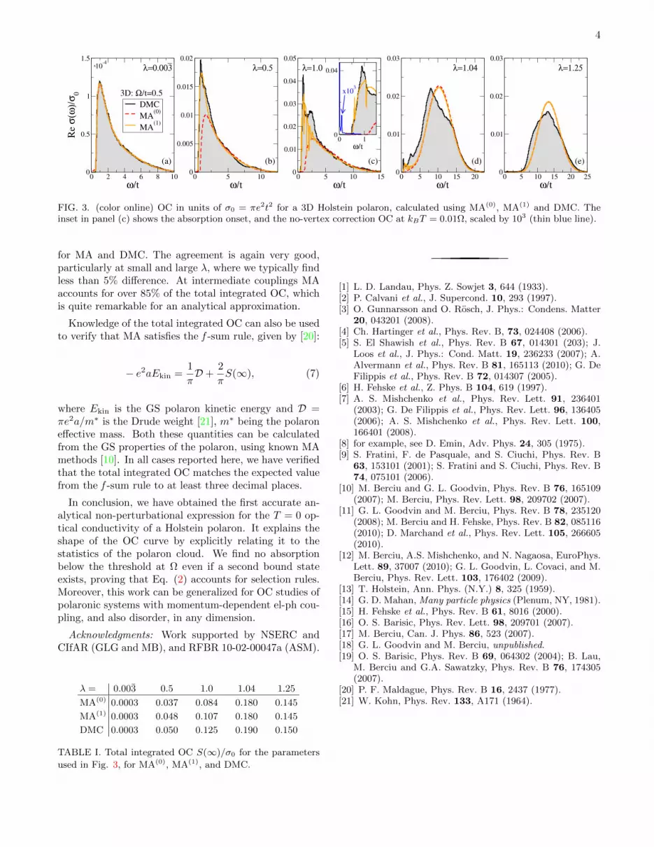
In Fig. 3, we plot the first, to our knowledge, com-plete set of OC curves reported for a 3D Holstein po-laron, using both MA and DMC methods. On the whole,the agreement is excellent, especially between MA(1) andDMC. We find that MA(1) captures all the qualitativefeatures of the full OC, as well as being able to resolvefiner structure near the absorption onset. In particu-lar, the “shoulder” that develops on the low-energy endof the OC spectrum could never be captured with per-turbational methods. In the asymptotic λ → 0,∞ lim-its the curves are nearly indistinguishable, as expectedsince MA becomes exact in these limits. In the crossoverregime λ ∼ 1, the differences between MA(0) and MA(1)

are largest, as are those between MA and DMC results.Nevertheless, MA does a good job overall, especially con-sidering that it is an efficient analytical approximation.

The shapes of the OC curves can now be understoodusing Eq. (2) and the data shown in Figs. 1 and 2. Forsmall λ, Pn=1 is dominant and the OC is basically pro-portional to fn=1(ω). Indeed, its rich structure is clearlyvisible in the OC, as is its threshold ωth = Ω. The n ≥ 2terms serve only to alter the high-energy tail. In the smallpolaron limit, however, Pn=1 → 0 and the OC is domi-nated by large n contributions. Since these fn(ω) curveshave similar shapes and are shifted by Ω with respect toone other, the OC mirrors the LF Poissonian distributionof Pn. The peak location is also in good agreement with

0

0.02

0.04

0.06

0.08

0.1

f n(ω

)

n=1n=2n=3n=4

0

0.02

0.04

0.06

0.08

0.1

f n(ω

)

n=1, MA(0)

0 4 8 12 16

ω/t

0

0.02

0.04

0.06

0.08

0.1

f n(ω

)

λ=0.003

3D: Ω/t=0.5

λ=1.0

MA(1)

λ=1.25

(a)

(b)

(c)

_

FIG. 2. (color online) MA(1) functions f(1)n (ω), for (a) small,

(b) medium, and (c) large el-ph coupling, at Ω/t = 0.5, η =

0.005 in 3D. Also shown is f(0)n=1(ω) (dashed line).

2|E0| = 12λt, expected as λ → ∞ [8]. This is becausewhen the electron is moved to a neighboring site by op-tical absorption, it loses the polaronic binding energy E0

and it also leaves behind excited phonons with the sameenergy. The structure of our expression (2) proves thatnot only the peak energy, but the very shape of the OC

curve is determined by the probabilities P(i)n . In 1D (not

shown), the fn(ω) functions are more peaked and indi-vidual contributions can be seen in the OC, as Ω-spacedkinks. The agreement with available 1D numerical datais of similar quality with that of Fig. 3 [18].

Consider now the DMFT-like no-vertex correction ap-proximation, in which the two-particle Green’s functionin Eq. (3) is replaced by a convolution of polaron spec-tral weights (for details, see the supplementary material).The scaled result for λ = 1, kBT = 0.01Ω, is shownin Fig. 3(c). A prominent feature is the peak (markedby arrow) below ωth, in agreement with low-T data inRef. [9], where it was identified as an excitation fromthe GS into the first bound-state. Indeed, the peak is at∼ 0.12t, their energy difference. The peak likely vanishesat T = 0, η = 0, however this shows that a naive con-sideration of the convolution may lead to a qualitativelywrong idea of the OC structure. DMC and MA resultsdo not show this peak, although the second bound stateis visible in their spectral weight (see the supplementarymaterial). Its absence implies a vanishing matrix elementin Eq. (4), likely due to the different symmetry of thepolaron wavefunction in the two states [19]. Clearly, Eq.(2) properly accounts for such selection rules. More anal-ysis is provided in the supplementary material found atthe end of this article.

To further prove the accuracy of MA, we compare inTable I the total integrated OC, S(∞) =

∫∞0dω σ(ω),

4

0 2 4 6 8 10

ω/t

0

0.5

1

1.5

Re σ

(ω)/

σ0

DMC

MA(0)

MA(1)

0 5 10

ω/t

0

0.005

0.01

0.015

0.02

0 5 10 15

ω/t

0

0.01

0.02

0.03

0.04

0.05

0 5 10 15 20

ω/t

0

0.01

0.02

0.03

0 5 10 15 20 25

ω/t

0

0.01

0.02

0.03

0 1

ω/t

0

0.04

(a) (b) (c) (d)

λ=0.003 λ=0.5 λ=1.0 λ=1.04 λ=1.25

(e)

_10

-4x

3D: Ω/t=0.5 x103

FIG. 3. (color online) OC in units of σ0 = πe2t2 for a 3D Holstein polaron, calculated using MA(0), MA(1) and DMC. Theinset in panel (c) shows the absorption onset, and the no-vertex correction OC at kBT = 0.01Ω, scaled by 103 (thin blue line).

for MA and DMC. The agreement is again very good,particularly at small and large λ, where we typically findless than 5% difference. At intermediate couplings MAaccounts for over 85% of the total integrated OC, whichis quite remarkable for an analytical approximation.

Knowledge of the total integrated OC can also be usedto verify that MA satisfies the f -sum rule, given by [20]:

− e2aEkin =1

πD +

2

πS(∞), (7)

where Ekin is the GS polaron kinetic energy and D =πe2a/m∗ is the Drude weight [21], m∗ being the polaroneffective mass. Both these quantities can be calculatedfrom the GS properties of the polaron, using known MAmethods [10]. In all cases reported here, we have verifiedthat the total integrated OC matches the expected valuefrom the f -sum rule to at least three decimal places.

In conclusion, we have obtained the first accurate an-alytical non-perturbational expression for the T = 0 op-tical conductivity of a Holstein polaron. It explains theshape of the OC curve by explicitly relating it to thestatistics of the polaron cloud. We find no absorptionbelow the threshold at Ω even if a second bound stateexists, proving that Eq. (2) accounts for selection rules.Moreover, this work can be generalized for OC studies ofpolaronic systems with momentum-dependent el-ph cou-pling, and also disorder, in any dimension.

Acknowledgments: Work supported by NSERC andCIfAR (GLG and MB), and RFBR 10-02-00047a (ASM).

λ = 0.003 0.5 1.0 1.04 1.25

MA(0) 0.0003 0.037 0.084 0.180 0.145

MA(1) 0.0003 0.048 0.107 0.180 0.145

DMC 0.0003 0.050 0.125 0.190 0.150

TABLE I. Total integrated OC S(∞)/σ0 for the parameters

used in Fig. 3, for MA(0), MA(1), and DMC.

[1] L. D. Landau, Phys. Z. Sowjet 3, 644 (1933).[2] P. Calvani et al., J. Supercond. 10, 293 (1997).[3] O. Gunnarsson and O. Rosch, J. Phys.: Condens. Matter

20, 043201 (2008).[4] Ch. Hartinger et al., Phys. Rev. B, 73, 024408 (2006).[5] S. El Shawish et al., Phys. Rev. B 67, 014301 (203); J.

Loos et al., J. Phys.: Cond. Matt. 19, 236233 (2007); A.Alvermann et al., Phys. Rev. B 81, 165113 (2010); G. DeFilippis et al., Phys. Rev. B 72, 014307 (2005).

[6] H. Fehske et al., Z. Phys. B 104, 619 (1997).[7] A. S. Mishchenko et al., Phys. Rev. Lett. 91, 236401

(2003); G. De Filippis et al., Phys. Rev. Lett. 96, 136405(2006); A. S. Mishchenko et al., Phys. Rev. Lett. 100,166401 (2008).

[8] for example, see D. Emin, Adv. Phys. 24, 305 (1975).[9] S. Fratini, F. de Pasquale, and S. Ciuchi, Phys. Rev. B

63, 153101 (2001); S. Fratini and S. Ciuchi, Phys. Rev. B74, 075101 (2006).

[10] M. Berciu and G. L. Goodvin, Phys. Rev. B 76, 165109(2007); M. Berciu, Phys. Rev. Lett. 98, 209702 (2007).

[11] G. L. Goodvin and M. Berciu, Phys. Rev. B 78, 235120(2008); M. Berciu and H. Fehske, Phys. Rev. B 82, 085116(2010); D. Marchand et al., Phys. Rev. Lett. 105, 266605(2010).

[12] M. Berciu, A.S. Mishchenko, and N. Nagaosa, EuroPhys.Lett. 89, 37007 (2010); G. L. Goodvin, L. Covaci, and M.Berciu, Phys. Rev. Lett. 103, 176402 (2009).

[13] T. Holstein, Ann. Phys. (N.Y.) 8, 325 (1959).[14] G. D. Mahan, Many particle physics (Plenum, NY, 1981).[15] H. Fehske et al., Phys. Rev. B 61, 8016 (2000).[16] O. S. Barisic, Phys. Rev. Lett. 98, 209701 (2007).[17] M. Berciu, Can. J. Phys. 86, 523 (2007).[18] G. L. Goodvin and M. Berciu, unpublished.[19] O. S. Barisic, Phys. Rev. B 69, 064302 (2004); B. Lau,

M. Berciu and G.A. Sawatzky, Phys. Rev. B 76, 174305(2007).

[20] P. F. Maldague, Phys. Rev. B 16, 2437 (1977).[21] W. Kohn, Phys. Rev. 133, A171 (1964).

5

SUPPLEMENTARY MATERIAL

Calculation of the matrix elements within MA(0)

First, we need to calculate the generalized single par-ticle Green’s functions:

Fnm(q,Q, ω) = 〈−q, n|cqG(ω)c†Q| −Q,m〉 (8)

where

| − q, n〉 =1√N

∑i

e−iq·Ri(b†i )n|0〉 (9)

We use Dyson’s identity G(ω) = G0(ω) + G(ω)V G0(ω)where V is the el-ph interaction and G0(ω) is the re-solvent for H0 = H − V , plus the MA(0) one-sitecloud restriction, to find Fnm(q,Q, ω) = G0(Q, ω −mΩ)[δq,Qδn,mn! + mgfn,m−1(q, ω) + gfn,m+1(q, ω)].Here, the free propagator is G0(k, ω) = (ω + iη −εk)−1, and fn,m(q, ω) = 1

N

∑Q Fnm(q,Q, ω) are par-

tial momentum averages related to the ones calculated inRef. [1]. They can therefore be calculated similarly; how-ever, they depend on q only through εq, therefore theyare even functions whose contribution to σ+(ω) vanishesafter the sum over q because of the odd prefactor sin qcoming from the current operator. As a result, withinMA(0) we can replace

Fnm(q,Q, ω)→ G0(Q, ω −mΩ)δq,Qδn,mn!

in Eq. (5). The delta functions remove the sums overm,Q. All that is left, then, is to find the residues|〈ψ0|c†q| − q, n〉|2. To achieve this, consider the gener-alized single-electron Green’s functions:

Fn(q, ω) = 〈0|ck=0G(ω)c†q| − q, n〉. (10)

These are also similar to the single particle Green’s func-tions calculated in Ref. [1], and can be calculated interms of continued fractions by the same means. WithinMA(0), they are equal to:

Fn(q, ω) =G0(q, ω − nΩ)

g0(ω − nΩ)An,1(ω)G(k = 0, ω). (11)

where G(k, ω) = 〈0|ckG(ω)c†k|0〉 is the usual single-particle polaron Green’s function, and we defineAn,k(ω) = An(ω)An−1(ω) · · ·Ak(ω) where the continu-ous fractions are [1, 2]:

An(ω) =ngg0(ω − nΩ)

1− gg0(ω − nΩ)An+1(ω)(12)

and

g0(ω) =1

N

∑q

G0(q, ω) (13)

is the momentum average of the bare propagator.On the other hand, from its Lehmann representation:

Fn(q, ω) =∑α

〈0|ck=0|ψα〉〈ψα|c†q| − q, n〉ω − Eα + iη

, (14)

so its residue for ω = E0, the GS energy, is the product〈0|ck=0|ψα〉〈ψα|c†q| − q, n〉. The first term is related tothe GS quasiparticle weight Z0, and the second is theoverlap that we need. It follows that:

〈ψ0|c†q| − q, n〉 =G0(q, ω − nΩ)

g0(ω − nΩ)

√Z0An,1(E0), (15)

The ω-independent part can be shown to be related tothe probability to have n-particles at the electron site inthe GS. In Ref. [3], these probabilities were found to be:

P (0)n =

Z0

n!|An,1(E0)|2 (16)

The ω-dependent terms can be grouped together with theone from Fnm(q,Q, ω) into the corresponding function

f(0)n (ω), whose expression is given in Eq. (6).The MA(1) calculations proceed along similar lines, but

are much more involved because of the enlarged basis.The full details will be presented in a longer publication.

The approximation of no current vertex corrections

The essence of this approximation is to replace the two-particle Green’s functions appearing in σ+(ω), namely

〈ψ0|c†QcQG(ω)c†qcq|ψ0〉, by a convolution of the single-particle spectral weights. The procedure is reviewed indetail in Ref. [4]. The regular part of the conductivity,at finite T and on a cubic lattice, is then found to be[their Eq. (19)]:

σ(ω) =4σ0

ωN

∑k

sin2 k

∫ ∞−∞

dω′A(k, ω′)A(k, ω + ω′)

× [f(ω′)− f(ω + ω′)] . (17)

Here A(k, ω) is the polaron spectral weight and f(ε) =(eβε+1)−1 is the Dirac function. This is the same formulaused in DMFT, see for example Eq. (3) in Ref. [5]. Thedifference is that in DMFT, the integral over the Brillouinzone is replaced by an integral over energies ε = εk (theyalso replace ω′ → ν). This explains the appearance ofthe density of states Nε of the free lattice, and of theDMFT vertex Φε which is the equivalent of the sin2 k inthe above equation. Of course, within DMFT one usesthe DMFT self-energy in the spectral weight.

In order to limit the quantitative differences of theDOS used in DMFT, which is for a Bethe lattice, whereasour other results are for a cubic lattice, we use Eq. (17)for a cubic lattice to test this approximation. Also, for

6

convenience, we use the MA self-energy in the spectralweight. This is simpler because in order to calculate theDMFT self-energy, one needs to go through iterations toreach self-consistency. In any event, the MA and DMFTself-energies are qualitatively and even quantitatively infairly good agreement, as shown in the Appendix of Ref.[1]. Moreover, it has been shown that the MA spectral

weights are very accurate, satisfying eight sum rules ex-actly (within MA(1)), therefore using the MA self-energyand its corresponding spectral weight can lead, at most,to modest quantitative differences.

Since the MA(1) self-energy is momentum-independent(momentum dependence appears only from the MA(2)

level), we can carry the integral over the Brillouin zoneas follows. We rewrite the spectral weights as

A(k, ω) = − 1

πG(k, ω) =

i

2π

[1

ω + iη − εk − Σ(ω)− 1

ω − iη − εk − Σ∗(ω)

]The product of two spectral weights will result in a sum of 4 terms that can be further factorized, for example:

1

ω′ + iη − εk − Σ(ω′)· 1

ω + ω′ + iη − εk − Σ(ω + ω′)

=1

ω − Σ(ω + ω′) + Σ(ω′)

[1

ω′ + iη − εk − Σ(ω′)− 1

ω + ω′ + iη − εk − Σ(ω + ω′)

(18)

As a result, the integral over the Brillouin zone now be-comes a simple momentum average of the bare propa-gator (with shifted frequency) times the sin2 kx term.One integral can be done analytically, and the other twonumerically like other similar momentum averages cal-culated for MA(2), see Ref. [1]. One is then left withevaluating the integral over ω′ numerically as well.

One can approach the T = 0 limit either directly byreplacing the Fermi-Dirac distribution with a Heavisidefunction, as done in Ref. [4]; or by calculating the T → 0limit of the ratio detailed in Refs. [5, 6]. Either approachhas its own numerical challenges, and overall we find bothprocedures to be more time consuming than evaluatingour OC formula, even when the computationally trivialMA self-energy is used in the spectral weight. Note, also,that our OC formula is formulated directly for T = 0and therefore one needs not worry about how to properlyapproach this limit.

The k = 0 spectral weight for the polaron, at interme-diary coupling λ = 1, is shown in Fig. 4. The GS peakstill has considerable weight Z0 ∼ 0.5, and just aboveit we see the peak corresponding to the second boundstate, followed by the continuum and higher energy fea-tures. The rough expectation is that a convolution ofthis curve with itself will show a first peak when the twocurves are shifted by E1 − E0, the energy difference be-tween the two bound states; also, absorption into thecontinuum will appear for frequencies ω > Ω.

Thus, the naive expectation based on the convolutionis that as soon as the second bound state is formed, thereshould be absorption into it, at energies below the thresh-old Ω. This is also what is shown by the full DMFT calcu-lations at very low temperatures, see curve of Fig. 2 and

its interpretation from Fig. 3 in Ref. [5], in qualitativeagreement with our own calculation for kBT = 0.01Ω,shown in Fig. 3(c) of the main article.

In reality, very careful analysis suggests that the weightof this peak decreases monotonically with T , and there-fore at T = 0 it is very likely that this approach also pre-dicts no absorption below the threshold at Ω, in agree-ment with the DMC and MA approaches. Our under-standing of the disappearance of this peak is that it comesfrom the fact that the k = 0 convolution is multiplied bysin2 k, so strictly speaking there is no contribution tothe OC from the GS momentum, unless some “thermal

-7 -6.5 -6 -5.5 -5ω/t

0.0

0.5

1.0

A(k

=0,ω

)

GS 2nd

bound state

continuum

FIG. 4. Spectral weight A(k = 0, ω) for the 3D Holsteinpolaron, for λ = 1,Ω = 0.5t, η = 10−3. The GS energy isE0 = −6.65t, and the first bound state is at E1 = −6.53t.The continuum onset is visible at E0 + Ω.

7

broadening” is allowed at non-zero temperatures.Since the exact DMC calculation finds no such absorp-

tion into the second bound state at any λ, the matrixelement for this transition must be zero, likely becauseof the different symmetry of the phonon clouds in thetwo states, as discussed in detail for 1D systems in Ref.[7]. Clearly, our MA-based OC formula captures thisselection rule properly – note that the generalized single-particle Green’s functions that appear in it are differentfrom the Green’s function that gives the spectral weight.

On the other hand, there is nothing in the spectralweight that encodes the symmetry of the wavefunctionassociated with a bound state, for example one cannotdistinguish the parity of a state by looking at the plot ofthe spectral weight. Thus, it seems to us that generically,one should expect the convolution approximation to failto properly account for selection rules.

In fact, this statement can be tested in 1D, where asshown in Ref. [7], one may expect higher energy boundstates, some of which are optically active. In other mod-els, it has been suggested that there may even be bound-states below the continuum which are not visible in thespectral weight, because their quasiparticle weight van-ishes for symmetry reasons [8] – if such states are opti-cally active, absorption associated with them would cer-tainly not be predicted by the convolution approxima-tion. Such a study will be undertaken elsewhere, andshould clarify whether the agreement in 3D regardingthe lack of sub-threshold absorption in the no-currentvertex approximation is accidental, or it actually has amore robust explanation. In any event, this is probablysomewhat of an academic discussion, since such multiplebound states appear only at large effective couplings λwhere the bulk of the optical absorption is at very much

higher energies, and in measurements the very small sig-nal at the threshold may be buried in noise.

Be that as it may, to us it appears that besides be-ing numerically more difficult to evaluate and less testedin terms of its accuracy for sum rules etc, the no-currentvertex approximation also fails to provide the insight intothe overall evolution of the OC curves that is affordedby our new formula. Moreover, MA has already beendemonstrated to generalize very successfully to modelswhere the coupling depends on the phonon and elec-tron momentum, and we expect similar success in mod-eling their OC. Such models have strongly momentum-dependent self-energies, and are unlikely to be describedaccurately with a local-approximation like DMFT.

[1] M. Berciu and G. L. Goodvin, Phys. Rev. B 76, 165109(2007).

[2] M. Berciu, Phys. Rev. Lett. 97, 036402 (2006); G.L. Good-vin, M. Berciu, and G.A. Sawatzky, Phys. Rev. B 74,245104 (2006).

[3] M. Berciu, Can. J. Phys. 86, 523 (2007).[4] J. Loos, M. Hohenadler, A. Alvermann, H. Fehske, J.

Phys.: Cond. Matt. 19, 236233 (2007).[5] S. Fratini, F. de Pasquale, and S. Ciuchi, Phys. Rev. B

63, 153101 (2001).[6] S. Fratini and S. Ciuchi, Phys. Rev. B 74, 075101 (2006).[7] O. S. Barisic, Phys. Rev. B 69, 064302 (2004).[8] B. Lau, M. Berciu and G.A. Sawatzky, Phys. Rev. B 76,

174305 (2007).