operations-oriented performance measures for freeway
TRANSCRIPT
Technical Report Documentation Page 1. Report No. FHWA/TX-07/0-5292-1
2. Government Accession No.
3. Recipient's Catalog No. 5. Report Date November 2006 Published: April 2007
4. Title and Subtitle OPERATIONS-ORIENTED PERFORMANCE MEASURES FOR FREEWAY MANAGEMENT SYSTEMS: YEAR 1 REPORT
6. Performing Organization Code
7. Author(s) Robert E. Brydia, William H. Schneider, Stephen P. Mattingly, Melanie L. Sattler, and Auttawit Upayokin
8. Performing Organization Report No. 0-5292-1 10. Work Unit No. (TRAIS)
9. Performing Organization Name and Address Texas Transportation Institute The Texas A&M University System College Station, Texas 77843-3135
11. Contract or Grant No. Project 0-5292 13. Type of Report and Period Covered Technical Report: September 2005 to August 2006
12. Sponsoring Agency Name and Address Texas Department of Transportation Research and Technology Implementation Office P.O. Box 5080 Austin, Texas 78763-5080
14. Sponsoring Agency Code
15. Supplementary Notes Project performed in cooperation with the Texas Department of Transportation and the Federal Highway Administration. Project Title: Using Operations-Oriented Performance Measures to Support Freeway Management Systems URL: http://tti.tamu.edu/document/0-5292-1.pdf 16. Abstract This report describes the year 1 activities on the project titled “Using Operations-Oriented Performance Measures to Support Freeway Management Systems.” Work activities included a comprehensive statewide survey on the use of performance measurement, as well as the initial recommendation on both operations and emissions-oriented performance measures to use in support of daily operations. 17. Key Words Performance Measurement, Operations, Emissions
18. Distribution Statement No restrictions. This document is available to the public through NTIS: National Technical Information Service Springfield, Virginia 22161 http://www.ntis.gov
19. Security Classif.(of this report) Unclassified
20. Security Classif.(of this page) Unclassified
21. No. of Pages 100
22. Price
Form DOT F 1700.7 (8-72) Reproduction of completed page authorized
RESUBMITTAL

RESUBMITTAL
OPERATIONS-ORIENTED PERFORMANCE MEASURES FOR FREEWAY MANAGEMENT SYSTEMS: YEAR 1 REPORT
by
Robert E. Brydia Associate Research Scientist
Texas Transportation Institute
William H. Schneider Assistant Research Scientist
Texas Transportation Institute
Dr. Stephen P. Mattingly Assistant Professor
University of Texas at Arlington
Dr. Melanie L. Sattler Assistant Professor
University of Texas at Arlington
and
Auttawit Upayokin Graduate Assistant
University of Texas at Arlington
Report 0-5292-1 Project 0-5292
Project Title: Using Operations-Oriented Performance Measures to Support Freeway Management Systems
Performed in cooperation with the
Texas Department of Transportation and the
Federal Highway Administration
November 2006 Published: April 2007
TEXAS TRANSPORTATION INSTITUTE
The Texas A&M University System College Station, Texas 77843-3135
RESUBMITTAL

RESUBMITTAL

v
DISCLAIMER
This research was performed in cooperation with the Texas Department of Transportation
(TxDOT) and the Federal Highway Administration (FHWA). The contents of this report reflect
the views of the authors, who are responsible for the facts and the accuracy of the data presented
herein. The contents do not necessarily reflect the official view or policies of the FHWA or
TxDOT. This report does not constitute a standard, specification, or regulation.
RESUBMITTAL
vi
ACKNOWLEDGMENTS
This project was conducted in cooperation with TxDOT and FHWA. The authors
gratefully acknowledge the contributions of numerous persons who made the successful
completion of this guidebook possible.
Project Coordinator • Al Kosik, P.E., Traffic Operations Division, TxDOT Project Director • Fabian Kalapach, P.E., Traffic Operations Division, TxDOT
Project Monitoring Committee • Brian Stanford, P.E., Traffic Operations Division, TxDOT • Charles Koonce, P.E., Austin District, TxDOT
RTI Engineer • Wade Odell, P.E., Research and Technology Implementation Office, TxDOT
Contracts Manager • Sandra Kaderka, Research and Technology Implementation Office, TxDOT
RESUBMITTAL
vii
TABLE OF CONTENTS
Page LIST OF FIGURES ..................................................................................................................... ix LIST OF TABLES ........................................................................................................................ x PROJECT BACKGROUND........................................................................................................ 1
STATE OF THE PRACTICE IN FREEWAY TRAFFIC MANAGEMENT............................ 1 THE RESEARCH QUESTION.................................................................................................. 2 THE RESEARCH APPROACH ................................................................................................ 4 RESEARCH PROJECT TASKS ................................................................................................ 5
A BRIEF HISTORY OF PERFORMANCE MEASUREMENT............................................. 7 WILLIAM DEMING.................................................................................................................. 7 PERFORMANCE MEASUREMENT TODAY......................................................................... 9
Federal Government Usage..................................................................................................... 9 PERFORMANCE MEASUREMENT IN TRANSPORTATION.......................................... 11
WIDE-SCALE COMPARISONS............................................................................................. 11 PERFORMANCE MEASUREMENT IN TRANSPORTATION AGENCIES....................... 11 EXAMPLES OF PRIOR PERFORMANCE MEASUREMENT IMPLEMENTATIONS ..... 13 FACTORS AFFECTING THE USE OF PERFORMANCE MEASUREMENT IN TRANSPORTATION............................................................................................................... 15
PERFORMANCE MEASURES FOR TRANSPORTATION OPERATIONS .................... 17 LEVELS OF PERFORMANCE MEASUREMENT IN OPERATIONS ................................ 17 OPERATIONAL PERFORMANCE MEASURES USED IN TEXAS ................................... 19 PERFORMANCE MEASUREMENT QUESTIONNAIRE .................................................... 20
Overview of Performance Measures..................................................................................... 21 System-Wide Assessment – Operations ............................................................................... 25 Program (Inter-Agency) Assessment – Operations .............................................................. 28 Daily Operations Assessment – Operations.......................................................................... 29 Equipment/Facilities Assessment – Operations.................................................................... 30 Emissions-Based Performance Measurement....................................................................... 31 Closing Comments/Remarks ................................................................................................ 32
IMPLEMENTING PERFORMANCE MEASUREMENT .................................................... 35 PERFORMANCE MEASURES IN DAILY OPERATIONS .................................................. 35 TYPES OF PERFORMANCE MEASUREMENT .................................................................. 35
Input/Output/Outcome .......................................................................................................... 35 Goal-Based Classification..................................................................................................... 36
CHALLENGES OF PERFORMANCE MEASURES ............................................................. 37 What Makes A Good Measure?............................................................................................ 40 Keys to a Successful Program............................................................................................... 41
PERFORMANCE MEASUREMENT PROCESS ................................................................... 42 RECOMMENDED OPERATIONS PERFORMANCE MEASURES .................................. 45
HANDBOOK FOR DEVELOPING A TMC OPERATIONS MANUAL............................... 46 GUIDE TO EFFECTIVE FREEWAY PERFORMANCE MEASURES ................................ 47 NATIONAL TRANSPORTATION OPERATIONS COALITION ........................................ 49
Customer Satisfaction ........................................................................................................... 50
RESUBMITTAL
viii
Extent of Congestion – Spatial ............................................................................................. 51 Extent of Congestion – Temporal ......................................................................................... 51 Incident Duration .................................................................................................................. 51 Non-Recurring Delay............................................................................................................ 52 Recurring Delay .................................................................................................................... 52 Speed..................................................................................................................................... 52 Throughput – Person............................................................................................................. 52 Throughput – Vehicle ........................................................................................................... 53 Travel Time – Link ............................................................................................................... 53 Travel Time – Reliability...................................................................................................... 53 Travel Time – Trip................................................................................................................ 53
SUMMARY OF RECOMMENDED MEASURES ................................................................. 54 RECOMMENDED EMISSIONS PERFORMANCE MEASURES ...................................... 55
EVALUATING THE PERFORMANCE OF AMBIENT AIR QUALITY ............................. 55 IMPACTS OF AIR POLLUTION ON HUMAN HEALTH.................................................... 56
Carbon monoxide (CO)......................................................................................................... 56 Particulate Matter (PM) ........................................................................................................ 57 Nitrogen dioxide (NO2)......................................................................................................... 60 Lead (Pb)............................................................................................................................... 61 Sulfur Dioxide (SO2)............................................................................................................. 62 Ozone (O3) ............................................................................................................................ 63
AIR QUALITY STANDARDS AND THEIR APPLICATION .............................................. 64 APPLICATION OF AIR POLLUTION STANDARDS.......................................................... 67
Air Pollution Index ............................................................................................................... 67 Air Quality Health Index (AQHI)......................................................................................... 72
AIR POLLUTION MONITORING AND MEASUREMENT ................................................ 73 Ambient Concentration Monitoring...................................................................................... 73 Mobile Monitoring................................................................................................................ 78
EMISSION PERFORMANCE MEASURES........................................................................... 80 REFERENCES............................................................................................................................ 87
RESUBMITTAL
ix
LIST OF FIGURES Page Figure 1. Typical Response Scenario for a Traffic Incident. ......................................................... 2 Figure 2. Illustration of a Strategic Response to an Incident. ........................................................ 3 Figure 3. Illustration of Management Approach Utilizing Performance Measurement. ............... 9 Figure 4. Multi-Level Approach to Operational Performance Measures. ................................... 18 Figure 5. Use of Performance Measures in TxDOT ATMS........................................................ 20 Figure 6. Current/Future Areas of Performance Measurement Use. ........................................... 24 Figure 7. Motivation for Using Performance Measurement. ....................................................... 25 Figure 8. Typical Performance Measurement Process. ............................................................... 42
RESUBMITTAL
x
LIST OF TABLES Page Table 1. Response Rate and Frequency of Reporting for NCHRP 238 Survey(a). ...................... 13 Table 2. Geographic Basis for Reporting Performance Measures in NCHRP 238 Survey(a)...... 15 Table 3. Questions Asked in Part 1 of Performance Measurement Questionnaire...................... 21 Table 4. Questions Asked in Part 2 of Performance Measurement Questionnaire...................... 26 Table 5. Example Table for Listing Sample Performance Measures. ......................................... 27 Table 6. Questions Asked in Part 3 of Performance Measurement Questionnaire...................... 29 Table 7. Questions Asked in Part 4 of Performance Measurement Questionnaire...................... 30 Table 8. Questions Asked in Part 5 of Performance Measurement Questionnaire...................... 31 Table 9. Questions Asked in Part 6 of Performance Measurement Questionnaire...................... 32 Table 10. Questions Asked in Part 7 of Performance Measurement Questionnaire.................... 33 Table 11. Recommended Minimum Freeway Performance Measures........................................ 48 Table 12. Health Impacts Associated with Carboxyhemoglobin Blood Levels. ......................... 56 Table 13. Nationwide Primary PM10 Emission Estimations from Mobile and Stationary Sources
from 1985 to 1993................................................................................................................. 59 Table 14. Epidemiologic Associations of Increments of Daily Particulate Concentrations........ 60 Table 15. Health Impacts of Particulate Matter. .......................................................................... 60 Table 16. Health Impacts of Nitrogen Dioxide............................................................................ 61 Table 17. Human Health and Vegetation Impacts of Sulfur Dioxide.......................................... 63 Table 18. Health Impacts of Ozone. ............................................................................................ 64 Table 19. U.S. Federal Primary and Secondary NAAQS. ........................................................... 65 Table 20. Federal PSD Concentration Increments....................................................................... 66 Table 21. Air Quality Classifications for Ozone. ........................................................................ 66 Table 22. AQI Values and Air Quality Descriptor. ..................................................................... 67 Table 23. Proposed Breakpoints for O3, PM2.5, PM10, CO, and SO2 Sub-Indices....................... 70 Table 24. Air Quality Index (AQI): Ozone.................................................................................. 70 Table 25. Air Quality Index (AQI): Particle Pollution. ............................................................... 71 Table 26. Air Quality Index (AQI): Carbon Monoxide (CO)...................................................... 71 Table 27. Air Quality Index (AQI): Sulfur Dioxide (SO2). ......................................................... 72 Table 28. Human Health Impacts Based on AQHI Scales. ......................................................... 73 Table 29. Summary Table of National Ambient Air Monitoring Networks................................ 75 Table 30. Methods for Pollutant Measurement............................................................................ 77 Table 31. Monitoring Site Scales................................................................................................. 78 Table 32. Monitoring Site Criteria............................................................................................... 78 Table 33. Emissions Performance Measures. .............................................................................. 82 Table 33. Emissions Performance Measures (cont)..................................................................... 83 Table 34. Emissions Performance Measures Applicable to Transportation. ............................... 84 Table 35. Evaluation of Emission Performance Measures Applicable to Transportation. .......... 86
RESUBMITTAL
1
PROJECT BACKGROUND
STATE OF THE PRACTICE IN FREEWAY TRAFFIC MANAGEMENT
The root concept underlying Freeway Traffic Management, as stated in the Freeway
Management and Operations Handbook, is to control, guide, and warn traffic to improve the
flow of people and goods on limited-access facilities(1).
Traffic management centers (TMCs) typically implement this concept, and traditional
operator tasks translate to the following:
• Monitor – observe traffic conditions and watch for abnormal or incident conditions,
• Respond – prepare and initiate actions using field-based infrastructure, and
• Disseminate – assemble and provide information to responders, drivers on the
roadway, and the public, using available communication means.
A typical response for managing an incident may be a multi-faceted approach of shutting
down a lane, sending an emergency response unit, implementing traffic diversion in the area, and
disseminating the information to the local region.
Actions to be taken in response to a situation on the roadway are typically well defined.
Effecting a control decision to change the traffic situation is not a decision that is made on a
whim. In many TMCs, experienced traffic engineers have created a database of standard
response strategies based on such items as type of incident, location, lanes affected, and traffic
level. In other locations, experienced operators use historical knowledge and experience to
decide what actions to take to respond to a situation on the freeway. In both cases, decisions,
and actions, are triggered only by a careful examination and verification of the roadway data.
Once a response is initiated, it is followed to the conclusion and the incident or alarm
situation is remedied and traffic has returned to normal patterns. Operators then go back to their
normal routine of monitoring the conditions and waiting for the next situation that requires their
attention. In most situations, that’s where the state of the practice stops for freeway
management.
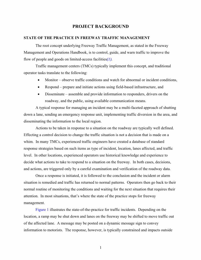
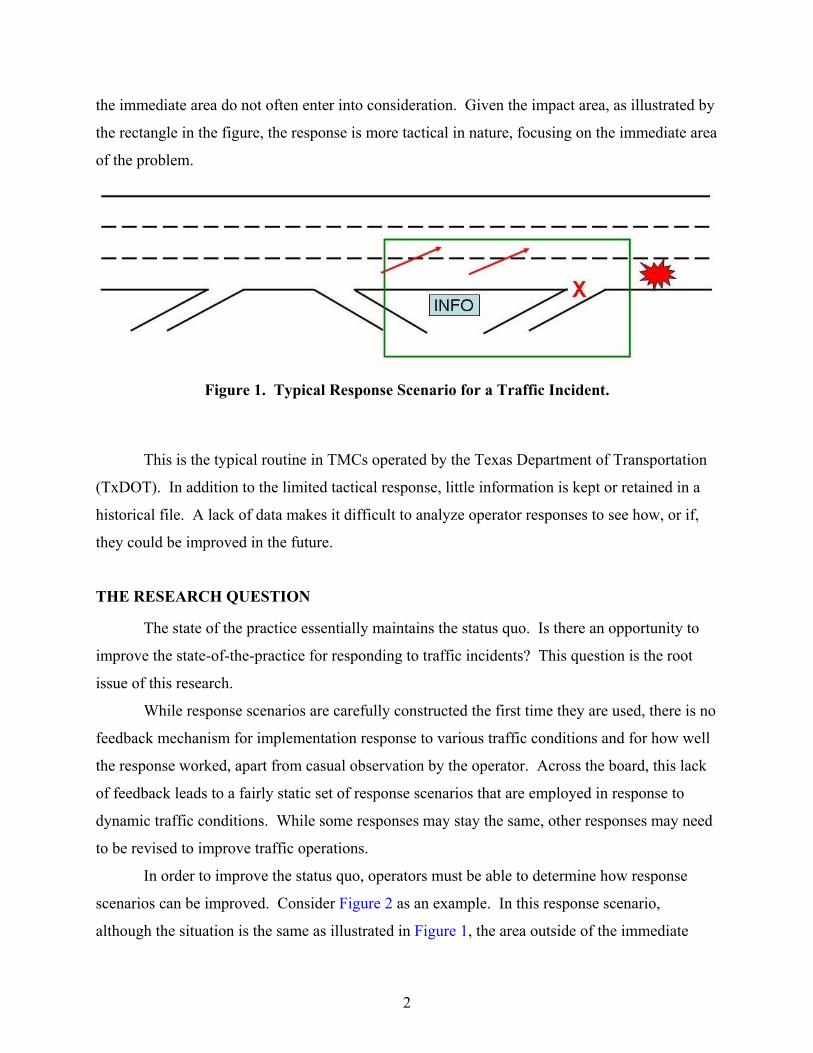
Figure 1 illustrates the state-of-the-practice for traffic incidents. Depending on the
location, a ramp may be shut down and lanes on the freeway may be shifted to move traffic out
of the affected lane. A message may be posted on a dynamic message sign to convey
information to motorists. The response, however, is typically constrained and impacts outside
RESUBMITTAL
2
the immediate area do not often enter into consideration. Given the impact area, as illustrated by
the rectangle in the figure, the response is more tactical in nature, focusing on the immediate area
of the problem.
Figure 1. Typical Response Scenario for a Traffic Incident.
This is the typical routine in TMCs operated by the Texas Department of Transportation
(TxDOT). In addition to the limited tactical response, little information is kept or retained in a
historical file. A lack of data makes it difficult to analyze operator responses to see how, or if,
they could be improved in the future.
THE RESEARCH QUESTION
The state of the practice essentially maintains the status quo. Is there an opportunity to
improve the state-of-the-practice for responding to traffic incidents? This question is the root
issue of this research.
While response scenarios are carefully constructed the first time they are used, there is no
feedback mechanism for implementation response to various traffic conditions and for how well
the response worked, apart from casual observation by the operator. Across the board, this lack
of feedback leads to a fairly static set of response scenarios that are employed in response to
dynamic traffic conditions. While some responses may stay the same, other responses may need
to be revised to improve traffic operations.
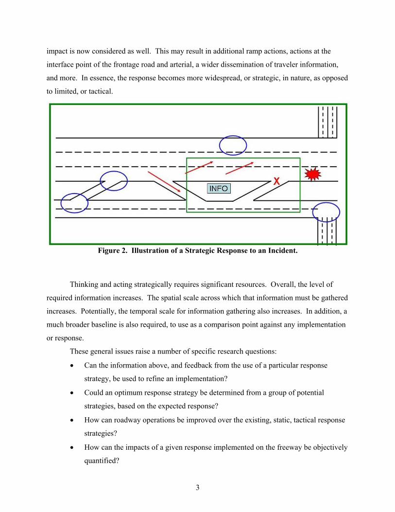
In order to improve the status quo, operators must be able to determine how response
scenarios can be improved. Consider Figure 2 as an example. In this response scenario,
although the situation is the same as illustrated in Figure 1, the area outside of the immediate
RESUBMITTAL
3
impact is now considered as well. This may result in additional ramp actions, actions at the
interface point of the frontage road and arterial, a wider dissemination of traveler information,
and more. In essence, the response becomes more widespread, or strategic, in nature, as opposed
to limited, or tactical.
Figure 2. Illustration of a Strategic Response to an Incident.
Thinking and acting strategically requires significant resources. Overall, the level of
required information increases. The spatial scale across which that information must be gathered
increases. Potentially, the temporal scale for information gathering also increases. In addition, a
much broader baseline is also required, to use as a comparison point against any implementation
or response.
These general issues raise a number of specific research questions:
• Can the information above, and feedback from the use of a particular response
strategy, be used to refine an implementation?
• Could an optimum response strategy be determined from a group of potential
strategies, based on the expected response?
• How can roadway operations be improved over the existing, static, tactical response
strategies?
• How can the impacts of a given response implemented on the freeway be objectively
quantified?
RESUBMITTAL
4
• What procedures or tools can be used to catalog the responses and compare them
without bias?
• How should a selection of strategies be made, from a range of possibilities?
• What type of strategies can be incorporated in this approach?
• What are the data requirements for this approach?
• How can TxDOT and TMCs utilize this approach to improve operations?
Overall, the goal of the project is to create a process that can quantitatively analyze an
implemented response and provide inputs into an assessment methodology to determine the best
response. The goal of the project is not to determine which strategy is most effective in what
situation.
THE RESEARCH APPROACH
Traditionally, one of the standard means for assessing the effectiveness of a strategy is to
use the concepts of performance measurement. A common definition for performance
measurement is “the use of statistical evidence to determine progress towards specific defined
organizational objectives” (2).
In other applications, performance measurement is used in real time to evaluate situations
such as production line quality. The state of the practice in traffic operations, however, is that
performance measurement for real-time operational assessment is not done, other than TMCs
that may compute a level of service (LOS) or similar measures, for an operator display. There
are no systems in Texas and no known systems nationally where performance measurement
concepts are used in combination with an assessment process to determine the benefits of
specific implements or provide a mechanism for choosing between multiple strategies.
It is reasonable to examine whether performance measurement techniques could be
applied to freeway management as well. The basic assumptions of the research are:
• Performance measurement can be applied to the problem at hand, namely to measure the
impacts of changing strategies on the roadway,
• Performance measurement can be used within an assessment methodology to understand
the implications of choosing a particular strategy, and
• Performance measurement can be examined for application to both operational and
emissions-based strategies.
RESUBMITTAL
5
RESEARCH PROJECT TASKS
To answer the questions, the researchers developed the following nine task workplan:
1. Assess Methodology for Current Operational Decisions – capture any performance
measurement process in current use.
2. Determine Operational Performance Measures to Support Freeway Strategies – prepare
a candidate list of operational performance measures.
3. Determine Emissions Performance Measures to Support Freeway Strategies – prepare a
candidate list of emissions-based performance measures.
4. Assess Requirements for Performance Measurement Systems – assess the requirements
for utilizing candidate performance measures.
5. Document Year 1 Progress – prepare a progress report of project status.
6. Construct Performance Measurement Based Methodology for Evaluating Multiple
Strategies – develop framework for assessing multiple strategies.
7. Design Prototype ATMS Displays – develop prototype screens for utilizing the
performance measurement methodology and measures within a advanced transportation
management software (ATMS) package.
8. Develop Concept of Operations – prepare a document highlighting users, data needs,
uses, and data flows for using performance measurement within ATMS.
9. Document Research Results – prepare a final, comprehensive project report.
Tasks 1 through 5 were performed in the first year of the research project and are the
subject of this report. Tasks 6 through 9 will be performed in the second and final year of the
research project.
RESUBMITTAL

RESUBMITTAL
7
A BRIEF HISTORY OF PERFORMANCE MEASUREMENT
Prior to detailing the results of the individual tasks, it is important to step back and
understand the broad scope of performance measurement. Performance measurement has been
applied to numerous applications across many different fields of study. The application of these
techniques for real-time traffic operations is the basis of this research. It is appropriate to be
aware of the history of performance measurement to gauge how the field has developed to
current applications.
WILLIAM DEMING
William Edwards Deming is often stated to be the father of performance measurement.
Deming was born in Sioux City, Iowa, in October 1900. He graduated from the University of
Wyoming as an engineer and in 1928 completed his studies for a Ph.D. from Yale University.
Upon completion of his degree, Deming went to work for the United States government as a
mathematical physicist.
Over the course of time, Deming developed both an interest in and understanding of the
use of statistical methods to analyze experimental data. He applied these skills in his work at the
U.S. Department of Agriculture (USDA) and later at the National Bureau of Standards. He also
continued his studies in statistics at University College, the University of London. In 1939,
Deming accepted a position as Head Mathematician and Advisor in Sampling at the U.S. Census
Bureau in preparation for the 1940 census. The 1940 census was the first census to employ
sampling techniques in lieu of the previous approach of counting everyone. In 1943, Deming
published a book Statistical Adjustment of Data that detailed the application of least-squares
regression techniques to various data issues. Leaving the Census Bureau in 1946, Deming
became a consultant for statistical studies, which he continued to his death in 1993. At the same
time, he also joined the faculty of New York University, lecturing in survey sampling and quality
control (3).
In 1947, Deming was asked by the Japanese government to help prepare for the 1951
census. As part of that work, he gave a dozen lectures on statistical and quality control
techniques. Combined, these techniques became known as Total Quality Management (TQM).
TQM incorporates concepts of product quality, process control, quality assurance, and quality
RESUBMITTAL
8
improvement. Deming taught TQM techniques to Japanese industries, most notably the
automobile industry. He is credited with significantly helping the country turn around from
World War II and embrace the concepts of producing quality products in a new, more global
economy (4).
It is important to understand that Deming’s work and teachings were not just about
statistics or quality control. In reality, the core of his teaching was about management. By
embracing what the customer wanted and designing a continuous process to create that product
with unsurpassed quality, the focus changed from quotas to customer satisfaction, from results to
methods. At the foundation of this continual evaluation of quality was the collection of data
gathered by a scientific approach and tools. Deming predicted that adoption of his techniques
would significantly improve Japanese market share within five years. History shows that change
occurred in some market sectors in as little as four years (5).
Deming’s work did not become widely accepted in the United States until the 1980s.
Whereas the Japanese industries were focusing on what their customers wanted and then
building that with unsurpassed quality, American industries had focused on traditional
management methods and the use of quotas and the chain of command. American industries had
to embrace TQM as a philosophy that integrates all functions for the sole purpose of meeting
customer needs and expectations. The overall process can be viewed as a multi-step path toward
better business (6):
1. improve product quality,
2. product costs decrease,
3. employee productivity increases,
4. company (and products) gain additional market share, and
5. company prospers.
As stated previously, the hallmark of this approach was the continual evaluation of
quality, using data gathered with scientific methods and tools. Over time, this benchmarking
process and the TQM principles became known as performance measurement.
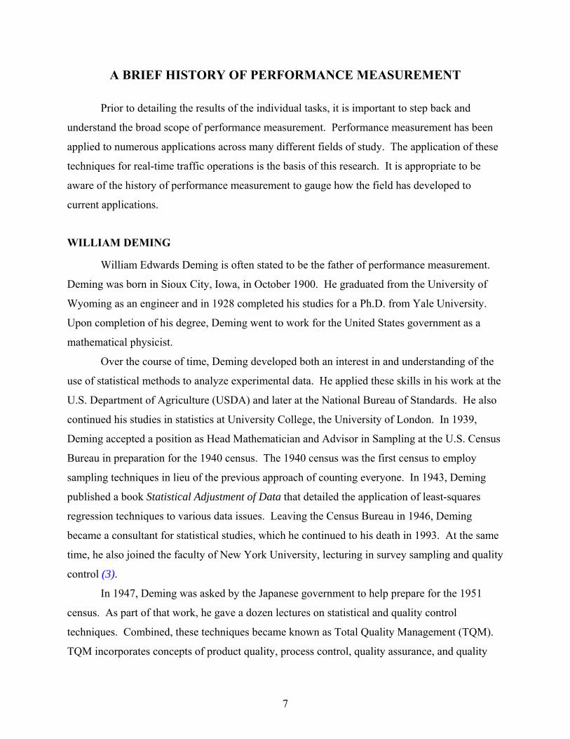
Pictorially, the process can be expressed as shown in Figure 3. Performance
measurement becomes the critical link in not only meeting the initial customer focus but also as
part of an iterative evaluation from the strategic planning process to keep the customer focus at
the forefront of all activities.
RESUBMITTAL
9
Figure 3. Illustration of Management Approach Utilizing Performance Measurement.
PERFORMANCE MEASUREMENT TODAY
Although American industries and agencies were somewhat slower to establish TQM, or
performance measurement approaches, over time the concepts have caught on and have been
implemented as part of standard business practices.
Federal Government Usage
Perhaps the event that best highlighted the use of performance measurement as a
scientific and systematic assessment tool was a benchmark study released by the federal
government in 1997 (7). This study advocated the use of performance management across all
federal agencies and provided an overview, best practices summary, and framework to assist in
that process. Prior even to this study, however, the Chief Financial Officer’s (CFO) Act of 1990
required more than 20 major government agencies to appoint a CFO whose responsibilities
included periodic systematic performance measurement information, as established by Public
Law 101-576. The Government Performance and Results Act of 1993 also required strategic
performance and planning initiatives throughout many federal government agencies. The act
provided for a 7-year staged implementation of annual performance reporting of performance
against goals based on strategic 5-year plans (8). As of result of these pieces of legislation and
studies, performance measurement is now an integral part of many federal level government
agencies.
RESUBMITTAL

10
It should be recognized, however, that performance measurement is not simply the
process of collecting data and seeing if a benchmark or value has been met. Rather, performance
measurement is an overall management system which allows a business or agency to collect and
evaluate information for the purpose of achieving goals, increasing efficiency, and meeting
customer expectations.
RESUBMITTAL
11
PERFORMANCE MEASUREMENT IN TRANSPORTATION
As in other industries, the use of performance measures in transportation has been
common for some time. In fact, many of the basic tenets of transportation, such as capacity
analysis, are based on performance measures, although they are not commonly referred to in
those terms. The Highway Capacity Manual (9) has generally referred to these as measures of
effectiveness (MOEs). Density, speed, and volume have all been used as MOEs for different
types of analyses. In addition to transportation operations, performance measures are frequently
used in other areas of the transportation field, such as pavements, structures, right-of-way
(ROW) and utility work, and communications.
In fact, the use of performance measures to analyze systems is of critical importance to
transportation. Through consistent application and quantification of these measures, engineers
gain the ability to measure and compare situations across different times, areas, and scales.
WIDE-SCALE COMPARISONS
Performance measurement can be used on a wide scale to assess broad patterns and
results. One of the best-known wide-scale comparisons utilizing performance measurement data
is the Urban Mobility Study, published yearly by the Texas Transportation Institute (10). This
study examines congestion across 85 urban areas in the United States utilizing data from 1982
through 2003. The study provides an on-going basis for cataloging and understanding the extent
of mobility problems within the United States.
The main performance measure utilized in the study is the Travel Time Index (TTI),
which measures the ratio of the time for a trip taken in peak conditions to the time for the same
trip in off-peak conditions. As an example, a TTI of 1.4 means that a 30-minute trip in off-peak
conditions will take 42 minutes in peak conditions. While the travel time index is the main
performance measure utilized, the study includes many such measures and adds new measures
over time to help explain the trends in urban mobility.
PERFORMANCE MEASUREMENT IN TRANSPORTATION AGENCIES
The use of performance measurement methodologies by state department of
transportation (DOT) agencies has been commonplace for several years. DOTs such as
RESUBMITTAL
12
Pennsylvania, Wisconsin, New York, Texas, and Oregon, to name a few, have long had
performance measurement systems in place for various aspects of transportation. For many
DOTs, the Intermodal Surface Transportation Efficiency Act (ISTEA) of 1991 formalized the
need for performance measurement by requiring states to implement management systems for
several aspects of the transportation system, including:
• pavement management systems,
• bridge management systems,
• safety management systems,
• congestion management systems,
• public transportation management systems, and
• intermodal management systems (8).
As part of the research conducted for National Cooperative Highway Research Program
(NCHRP) Synthesis 238, a survey was utilized to collect performance measurement information
from state DOTs. The survey sought to identify where performance measurement was being
used across all modes of transportation, as well as examine the reporting characteristics in terms
of frequency and geographic basis. In particular, information was collected about the following
program areas:
• Multimodal Transportation,
• Highway Construction,
• Highway Maintenance,
• Traffic Safety,
• Public Transportation,
• Ferry Service,
• Aviation,
• Railroads,
• Ports and Waterways, and
• Licensing and Registration (8).
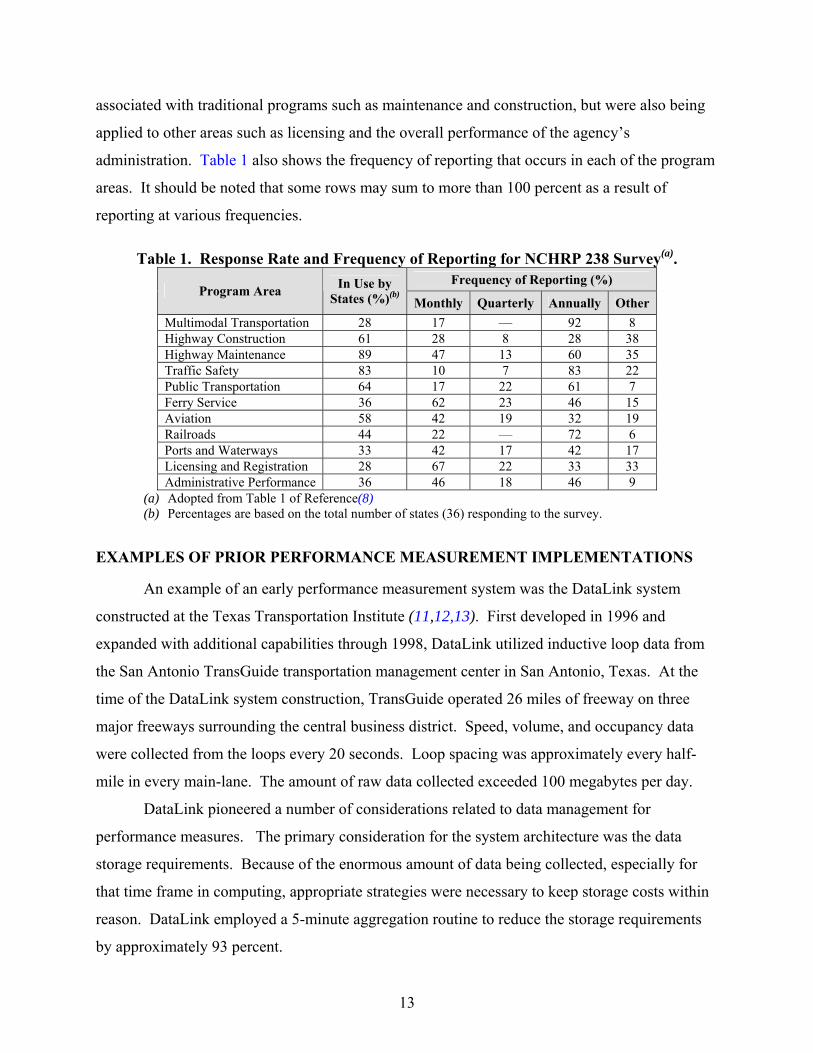
Table 1, adapted from Table 1 of the NCHRP synthesis study, shows that as of the 1997
publication date, performance measurement was gaining acceptance in many program areas
across the responding states. As might be expected, performance measures were more often
RESUBMITTAL
13
associated with traditional programs such as maintenance and construction, but were also being
applied to other areas such as licensing and the overall performance of the agency’s
administration. Table 1 also shows the frequency of reporting that occurs in each of the program
areas. It should be noted that some rows may sum to more than 100 percent as a result of
reporting at various frequencies.
Table 1. Response Rate and Frequency of Reporting for NCHRP 238 Survey(a). Frequency of Reporting (%)
Program Area In Use by States (%)(b) Monthly Quarterly Annually Other
Multimodal Transportation 28 17 — 92 8 Highway Construction 61 28 8 28 38 Highway Maintenance 89 47 13 60 35 Traffic Safety 83 10 7 83 22 Public Transportation 64 17 22 61 7 Ferry Service 36 62 23 46 15 Aviation 58 42 19 32 19 Railroads 44 22 — 72 6 Ports and Waterways 33 42 17 42 17 Licensing and Registration 28 67 22 33 33 Administrative Performance 36 46 18 46 9
(a) Adopted from Table 1 of Reference(8) (b) Percentages are based on the total number of states (36) responding to the survey.
EXAMPLES OF PRIOR PERFORMANCE MEASUREMENT IMPLEMENTATIONS
An example of an early performance measurement system was the DataLink system
constructed at the Texas Transportation Institute (11,12,13). First developed in 1996 and
expanded with additional capabilities through 1998, DataLink utilized inductive loop data from
the San Antonio TransGuide transportation management center in San Antonio, Texas. At the
time of the DataLink system construction, TransGuide operated 26 miles of freeway on three
major freeways surrounding the central business district. Speed, volume, and occupancy data
were collected from the loops every 20 seconds. Loop spacing was approximately every half-
mile in every main-lane. The amount of raw data collected exceeded 100 megabytes per day.
DataLink pioneered a number of considerations related to data management for
performance measures. The primary consideration for the system architecture was the data
storage requirements. Because of the enormous amount of data being collected, especially for
that time frame in computing, appropriate strategies were necessary to keep storage costs within
reason. DataLink employed a 5-minute aggregation routine to reduce the storage requirements
by approximately 93 percent.
RESUBMITTAL
14
In a similar consideration to the size of the overall storage, the desired storage and
retrieval capabilities necessitated the use of a relational database. Common desktop databases
could not handle the requirements of the system, and a larger enterprise-level database was
utilized. Specialized screening rules were developed to ensure data integrity within the database.
Performance measures identified the number of data elements used in the calculation to ensure
proper interpretation of the results.
The ability to easily access and work with the data contained in the database was a crucial
factor in making the system feasible. DataLink utilized an open-standards web interface to
provide access to and manipulation of the data within the system, eliminating the need for
specialized programming or database skills on the part of system user and expanding the ability
to use the system to anyone in the target agency. This highlights a key finding related to
performance measurement: The data should be available to those who need to use it and it
should not be difficult to find or develop.
In its most basic capabilities, DataLink output provided speed, volume, and occupancy
information at user-specified time intervals and locations. The aggregation techniques provide a
report on time periods from 5 minutes to 1 day. DataLink output also supported the calculation
of performance measures based on both lane and corridor aggregation techniques.
The DataLink system was research-based and explored a number of never-before
examined questions pertaining to large-scale data archiving activities within transportation. A
similar, but operational, system was constructed in Montgomery County, Maryland (14). Known
as DASH, or Data Acquisition and Hardware, the system utilized many of the same components
as DataLink. The system employed screening techniques for data integrity, automatically
updated itself as new detectors were brought on-line, updated new data once a day, and allowed
multiple end-user queries. DASH provided significant benefits to Montgomery County,
including the ability to collect and store more accurate and precise data, improve information
sharing throughout the agency, and reduce the need for supplementary traffic data collection.
Throughout the literature, a number of smaller-scale systems used performance measures
constructed from archived data to analyze more focused objectives. One such study performed
travel time analyses on the Katy Freeway in Houston, Texas (15). The objective was to quantify
travel any time savings on the toll lanes as compared to the main lanes. This study was not a
RESUBMITTAL
15
large-scale exercise but allowed development of an evaluation procedure and framework for
using the travel time savings information as a performance measure.
FACTORS AFFECTING THE USE OF PERFORMANCE MEASUREMENT IN TRANSPORTATION
While the data are a critical element of any performance measurement system, the
literature also shows other factors which must be considered. One critical factor in the
application of performance measurement is the geographic scale. Performance measures can be
constructed to look at global objectives, to focus on a detailed evaluation of any given
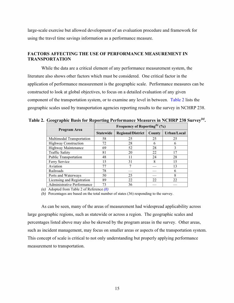
component of the transportation system, or to examine any level in between. Table 2 lists the
geographic scales used by transportation agencies reporting results to the survey in NCHRP 238.
Table 2. Geographic Basis for Reporting Performance Measures in NCHRP 238 Survey(a). Frequency of Reporting(b) (%)
Program Area Statewide Regional/District County Urban/Local
Multimodal Transportation 58 25 25 25 Highway Construction 72 28 6 6 Highway Maintenance 69 52 28 3 Traffic Safety 81 20 22 17 Public Transportation 48 11 24 28 Ferry Service 15 31 8 15 Aviation 77 7 — 13 Railroads 78 — — 6 Ports and Waterways 50 25 — 8 Licensing and Registration 89 22 22 22 Administrative Performance 73 36 — —
(a) Adopted from Table 2 of Reference (8) (b) Percentages are based on the total number of states (36) responding to the survey.
As can be seen, many of the areas of measurement had widespread applicability across
large geographic regions, such as statewide or across a region. The geographic scales and
percentages listed above may also be skewed by the program areas in the survey. Other areas,
such as incident management, may focus on smaller areas or aspects of the transportation system.
This concept of scale is critical to not only understanding but properly applying performance
measurement to transportation.
RESUBMITTAL

RESUBMITTAL
17
PERFORMANCE MEASURES FOR TRANSPORTATION OPERATIONS
Perhaps the aspect of transportation that has the largest impact on the daily lives of users
of the transportation system is that of operations. Transportation operations is a vast area of
programs and policies designed, in large part, to address the congestion on the nation’s highways
and improve the traveling conditions. Transportation operations include areas such as:
• arterial management,
• access management,
• congestion mitigation,
• corridor traffic management,
• emergency transportation operations,
• freeway management,
• freight analysis and management,
• real-time traveler information,
• road weather management,
• tolling and pricing opportunities,
• traffic analysis and simulation,
• travel demand management,
• traffic incident management,
• planned special events traffic management, and
• work zone management (16).
Despite the large number of programs and resources devoted to operations, Table 1 and Table 2
show that performance measurement is not in common use in this area.
LEVELS OF PERFORMANCE MEASUREMENT IN OPERATIONS
Similar to the other areas of transportation, the application of performance measurement
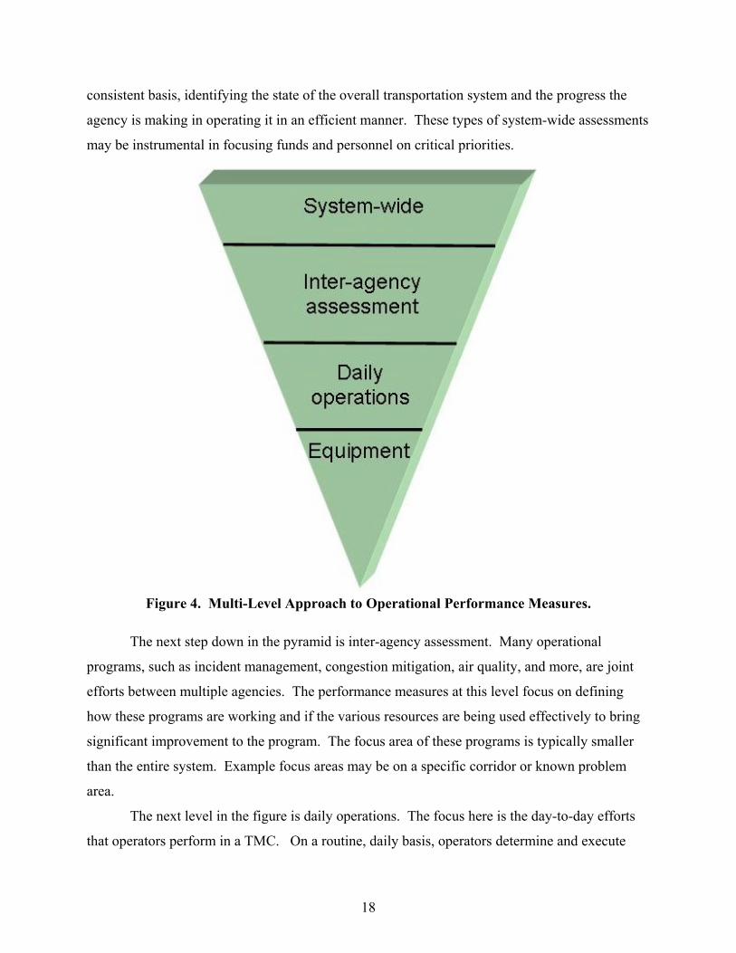
to operations can incorporate multiple scales or levels. Figure 4 [adopted from Figure 1-1 of
Reference (17)] illustrates this concept by showing a pyramidal approach to defining
performance measures. At the top of the figure is the largest level or area of measurement, the
system-wide assessment. This is the most global view of operations and serves a multitude of
purposes. For one, this may be the information that the public and elected officials receive on a
RESUBMITTAL
18
consistent basis, identifying the state of the overall transportation system and the progress the
agency is making in operating it in an efficient manner. These types of system-wide assessments
may be instrumental in focusing funds and personnel on critical priorities.
Figure 4. Multi-Level Approach to Operational Performance Measures.
The next step down in the pyramid is inter-agency assessment. Many operational
programs, such as incident management, congestion mitigation, air quality, and more, are joint
efforts between multiple agencies. The performance measures at this level focus on defining
how these programs are working and if the various resources are being used effectively to bring
significant improvement to the program. The focus area of these programs is typically smaller
than the entire system. Example focus areas may be on a specific corridor or known problem
area.
The next level in the figure is daily operations. The focus here is the day-to-day efforts
that operators perform in a TMC. On a routine, daily basis, operators determine and execute
RESUBMITTAL
19
responses based on inputs and execute strategies to keep traffic flowing. These responses and
strategies may be lane shifts, dynamic message sign postings, implementing changes in ramp
operations, or more. While the focus area of these actions is typically compressed, i.e., smaller
than an entire corridor, the potential impact area is much larger.
At the bottom of the pyramid are those measures that focus specifically on equipment or
very discrete elements of the transportation system. Typical applications at this level may
include items such as up-time, reliability, integrity of data, or more. Looking at these measures
should provide an overview sense of how the data collection, processing, storage, and calculation
components of performance measurement are working across the entire extent of transportation
operations.
OPERATIONAL PERFORMANCE MEASURES USED IN TEXAS
In the current state-of-the-practice, the use of performance measurement techniques
within TxDOT is minimal. Some areas use system-wide measures to convey information to the
public or elected officials. This is typically done as some sort of annual summary of conditions
or progress report.
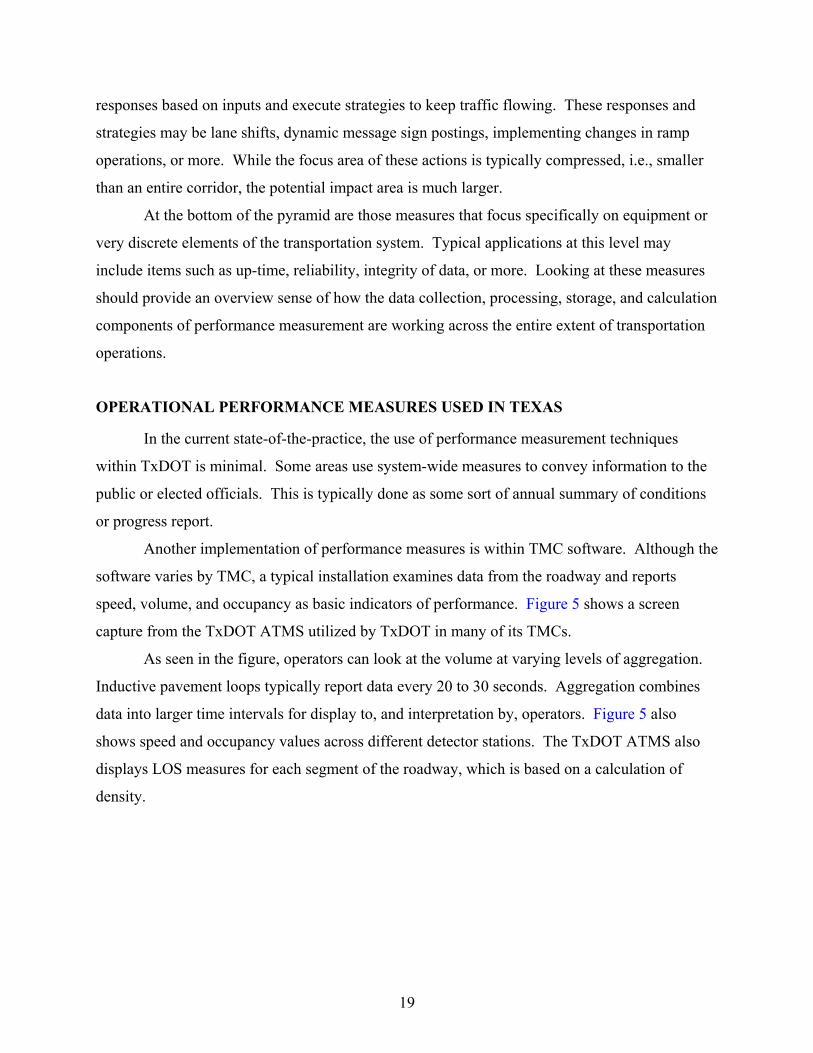
Another implementation of performance measures is within TMC software. Although the
software varies by TMC, a typical installation examines data from the roadway and reports
speed, volume, and occupancy as basic indicators of performance. Figure 5 shows a screen
capture from the TxDOT ATMS utilized by TxDOT in many of its TMCs.
As seen in the figure, operators can look at the volume at varying levels of aggregation.
Inductive pavement loops typically report data every 20 to 30 seconds. Aggregation combines
data into larger time intervals for display to, and interpretation by, operators. Figure 5 also
shows speed and occupancy values across different detector stations. The TxDOT ATMS also
displays LOS measures for each segment of the roadway, which is based on a calculation of
density.
RESUBMITTAL
20
Figure 5. Use of Performance Measures in TxDOT ATMS.
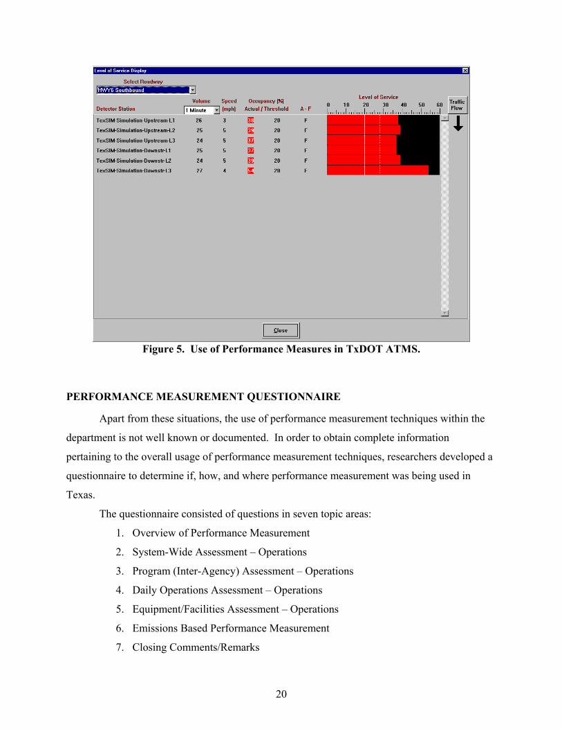
PERFORMANCE MEASUREMENT QUESTIONNAIRE
Apart from these situations, the use of performance measurement techniques within the
department is not well known or documented. In order to obtain complete information
pertaining to the overall usage of performance measurement techniques, researchers developed a
questionnaire to determine if, how, and where performance measurement was being used in
Texas.
The questionnaire consisted of questions in seven topic areas:
1. Overview of Performance Measurement
2. System-Wide Assessment – Operations
3. Program (Inter-Agency) Assessment – Operations
4. Daily Operations Assessment – Operations
5. Equipment/Facilities Assessment – Operations
6. Emissions Based Performance Measurement
7. Closing Comments/Remarks
RESUBMITTAL
21
The survey was administered via face-to-face or telephone interviews to six locations
within Texas, including:
• TransVista (El Paso),
• TransGuide (San Antonio),
• TranStar (Houston),
• DalTrans (Dallas),
• TransVision (Ft. Worth), and
• TxDOT Traffic Operations Headquarters (Austin, TX).
Each survey respondent was contacted initially via telephone or electronic mail and asked
to participate. The respondents were given an overview of the questionnaire and told that it
would take approximately 30 minutes to go through the questions. A scheduled time for the
interview was then set according to the schedule of the respondent.
These sites and their answers to the questionnaire provided a comprehensive look at the
use of performance measurement in Texas. Each of the following sections presents the questions
from the questionnaire and an overview of the results
Overview of Performance Measures
The scope of this section of the questionnaire was to introduce the concept of
performance measurement and get an understanding of where the respondent stood in terms of
knowledge of the subject and application of the general concepts within their agency
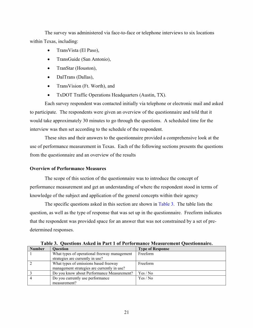
The specific questions asked in this section are shown in Table 3. The table lists the
question, as well as the type of response that was set up in the questionnaire. Freeform indicates
that the respondent was provided space for an answer that was not constrained by a set of pre-
determined responses.
Table 3. Questions Asked in Part 1 of Performance Measurement Questionnaire. Number Question Type of Response 1 What types of operational freeway management
strategies are currently in use? Freeform
2 What types of emissions based freeway management strategies are currently in use?
Freeform
3 Do you know about Performance Measurement? Yes / No 4 Do you currently use performance
measurement? Yes / No
RESUBMITTAL
22
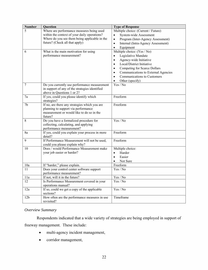
Number Question Type of Response 5 Where are performance measures being used
within the context of your daily operations? Where do you see them being applicable in the future? (Check all that apply)
Multiple choice: (Current / Future) • System-wide Assessment • Program (Inter-Agency Assessment) • Internal (Intra-Agency Assessment) • Equipment
6 What is the main motivation for using performance measurement?
Multiple choice: (Yes / No) • Legislative Mandate • Agency-wide Initiative • Local/District Initiative • Competing for Scarce Dollars • Communications to External Agencies • Communications to Customers • Other (specify)
7 Do you currently use performance measurement in support of any of the strategies identified above in Questions 1 or 2?
Yes / No
7a If yes, could you please identify which strategies?
Freeform
7b If no, are there any strategies which you are planning to support via performance measurement or would like to do so in the future?
Freeform
8 Do you have a formalized procedure for collecting, calculating, and applying performance measurement?
Yes / No
8a If yes, could you explain your process in more detail?
Freeform
9 If Performance Measurement will not be used, could you please explain why?
Freeform
10 Does / would Performance Measurement make your job easier or harder?
Multiple choice: • Harder • Easier • Not Sure
10a If “harder,” please explain. Freeform 11 Does your control center software support
performance measurement? Yes / No
11a If not, will it in the future? Yes / No 12 Is Performance Measurement covered in your
operations manual? Yes / No
12a If so, could we get a copy of the applicable sections?
Yes / No
12b How often are the performance measures in use revisited?
Timeframe
Overview Summary
Respondents indicated that a wide variety of strategies are being employed in support of
freeway management. These include:
• multi-agency incident management,
• corridor management,
RESUBMITTAL
23
• co-location of agencies,
• public information/outreach,
• dynamic message signs,
• lane control signals,
• data archiving,
• weather responsive condition alerts,
• high-occupancy vehicle/high-occupancy toll (HOV/HOT) lanes,
• ramp metering,
• traffic management centers,
• equipment maintenance database, and
• construction impact management.
The type and extent of the responses are a testament to the breadth of techniques being
employed across Texas to help manage and mitigate traffic situations. In contrast, for emissions
strategies, respondents indicated that a significantly smaller set of strategies is in use. The
predominant answer was ozone alert days. Even with this strategy, there are no real numbers to
support the strategy.
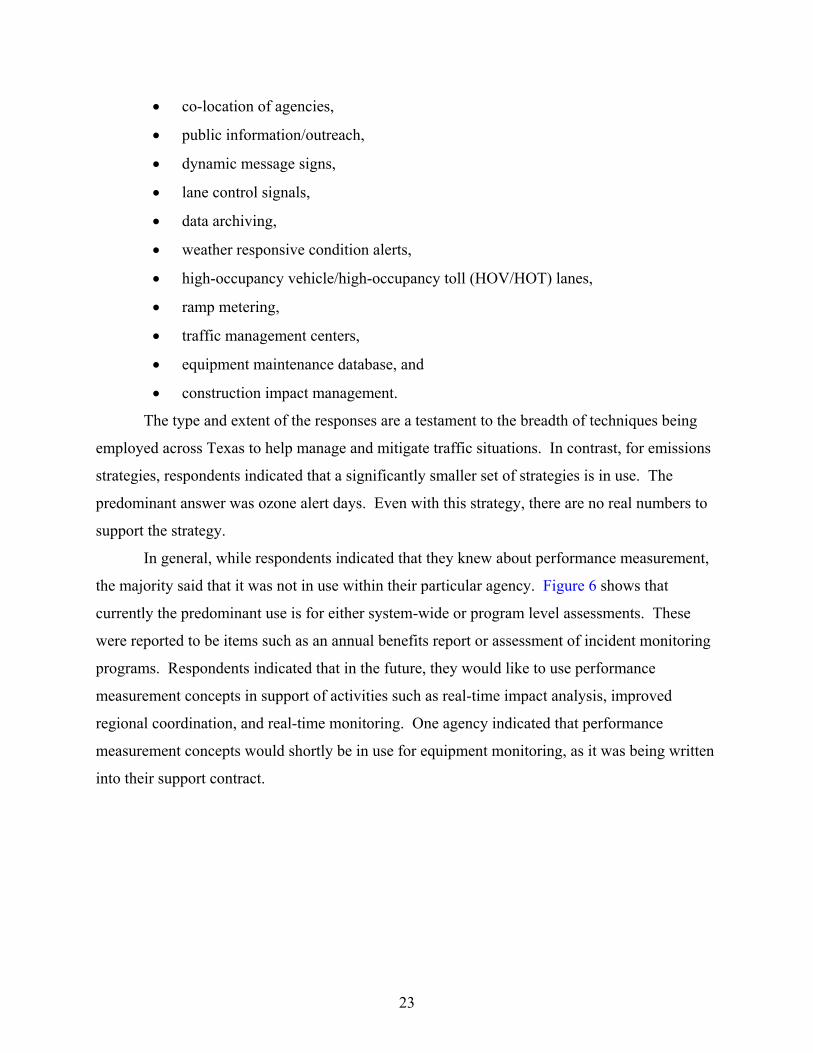
In general, while respondents indicated that they knew about performance measurement,
the majority said that it was not in use within their particular agency. Figure 6 shows that
currently the predominant use is for either system-wide or program level assessments. These
were reported to be items such as an annual benefits report or assessment of incident monitoring
programs. Respondents indicated that in the future, they would like to use performance
measurement concepts in support of activities such as real-time impact analysis, improved
regional coordination, and real-time monitoring. One agency indicated that performance
measurement concepts would shortly be in use for equipment monitoring, as it was being written
into their support contract.
RESUBMITTAL
24
0
1
2
3
4
5
6
Current Future
System Wide AssessmentProgram AssessmentDaily OperationsEquipment
Figure 6. Current/Future Areas of Performance Measurement Use.
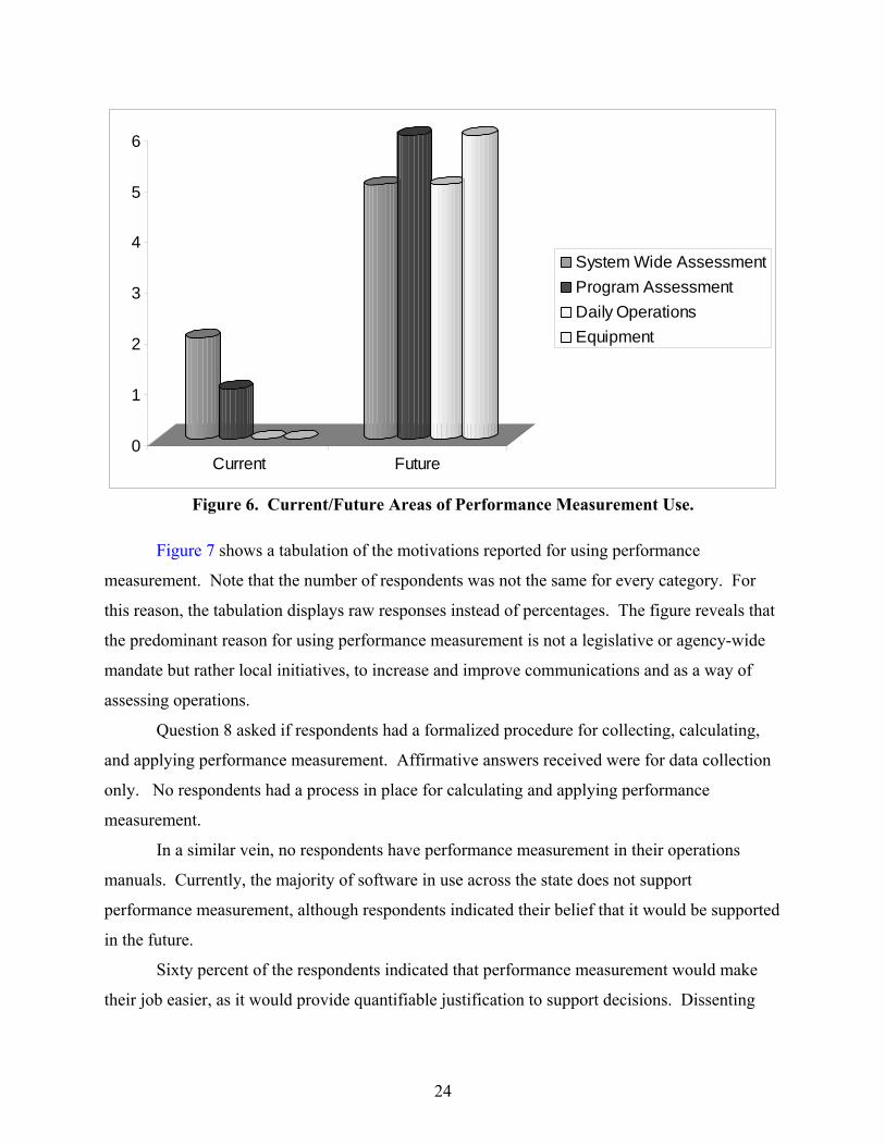
Figure 7 shows a tabulation of the motivations reported for using performance
measurement. Note that the number of respondents was not the same for every category. For
this reason, the tabulation displays raw responses instead of percentages. The figure reveals that
the predominant reason for using performance measurement is not a legislative or agency-wide
mandate but rather local initiatives, to increase and improve communications and as a way of
assessing operations.
Question 8 asked if respondents had a formalized procedure for collecting, calculating,
and applying performance measurement. Affirmative answers received were for data collection
only. No respondents had a process in place for calculating and applying performance
measurement.
In a similar vein, no respondents have performance measurement in their operations
manuals. Currently, the majority of software in use across the state does not support
performance measurement, although respondents indicated their belief that it would be supported
in the future.
Sixty percent of the respondents indicated that performance measurement would make
their job easier, as it would provide quantifiable justification to support decisions. Dissenting
RESUBMITTAL
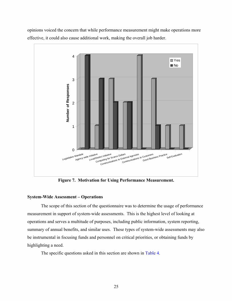
25
opinions voiced the concern that while performance measurement might make operations more
effective, it could also cause additional work, making the overall job harder.
0
1
2
3
4
Num
ber
of R
espo
nses
Legistlative Mandate
Agency-wide Initiative
Local/District Initiative
Competing for Scarce Dollars
Communications to External Agencies
Communications to Customers
Good Business PracticeSelf Evaluation
YesNo
Figure 7. Motivation for Using Performance Measurement.
System-Wide Assessment – Operations
The scope of this section of the questionnaire was to determine the usage of performance
measurement in support of system-wide assessments. This is the highest level of looking at
operations and serves a multitude of purposes, including public information, system reporting,
summary of annual benefits, and similar uses. These types of system-wide assessments may also
be instrumental in focusing funds and personnel on critical priorities, or obtaining funds by
highlighting a need.
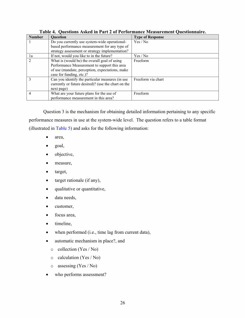
The specific questions asked in this section are shown in Table 4.
RESUBMITTAL
26
Table 4. Questions Asked in Part 2 of Performance Measurement Questionnaire. Number Question Type of Response 1 Do you currently use system-wide operational-
based performance measurement for any type of strategy assessment or strategy implementation?
Yes / No
1a If not, would you like to in the future? Yes / No 2 What is (would be) the overall goal of using
Performance Measurement to support this area of use (mandate, perception, expectations, make case for funding, etc.)?
Freeform
3 Can you identify the particular measures (in use currently or future desired)? (use the chart on the next page)
Freeform via chart
4 What are your future plans for the use of performance measurement in this area?
Freeform
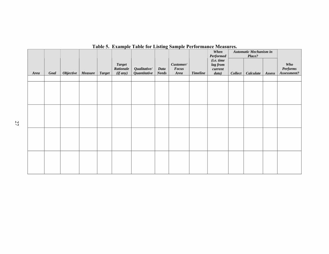
Question 3 is the mechanism for obtaining detailed information pertaining to any specific
performance measures in use at the system-wide level. The question refers to a table format
(illustrated in Table 5) and asks for the following information:
• area,
• goal,
• objective,
• measure,
• target,
• target rationale (if any),
• qualitative or quantitative,
• data needs,
• customer,
• focus area,
• timeline,
• when performed (i.e., time lag from current data),
• automatic mechanism in place?, and
o collection (Yes / No)
o calculation (Yes / No)
o assessing (Yes / No)
• who performs assessment?
RESUBMITTAL
27
Table 5. Example Table for Listing Sample Performance Measures. Automatic Mechanism in
Place?
Area Goal Objective Measure Target
Target Rationale (if any)
Qualitative/Quantitative
Data Needs
Customer/ Focus Area Timeline
When Performed (i.e. time lag from current data) Collect Calculate Assess
Who Performs
Assessment?
RE
SU
BM
ITT
AL
28
Researches requested these information items as direct support to future tasks in
the project.
System-Wide Assessment Summary
The responses to this section of the survey indicated that for the most part,
performance measurement to support system-wide assessments is not being used. This
corresponds to Figure 6, which indicated only a few current users. Measures that
respondents indicated as being in use include:
• travel time,
• travel speed,
• total delay,
• recurrent delay,
• no-recurrent delay,
• travel time index, and
• incident detection rate.
In general, the overall goal of using performance measurement for this area was to
evaluate actual performance against expectations, justify funding, or modify procedures
to improve the system.
Program (Inter-Agency) Assessment – Operations
The scope of this section of the questionnaire was to determine the usage of
performance measurement in support of program level, typically inter-agency, type of
operations. Performance measures at this level focus on defining how a program is
working and if the various resources are being used effectively to bring significant
improvement to the program. The focus area of these programs is typically smaller than
the entire system and may focus on a specific corridor or problem area.
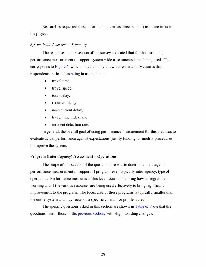
The specific questions asked in this section are shown in Table 6. Note that the
questions mirror those of the previous section, with slight wording changes.
RESUBMITTAL
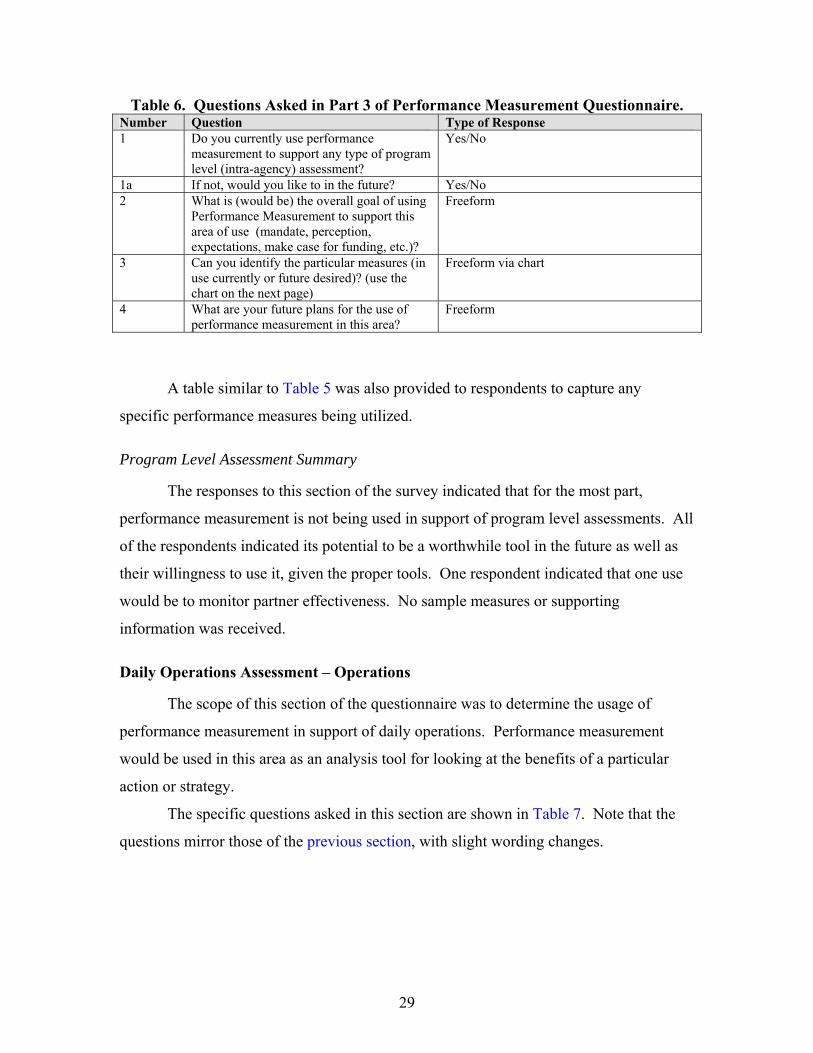
29
Table 6. Questions Asked in Part 3 of Performance Measurement Questionnaire. Number Question Type of Response 1 Do you currently use performance
measurement to support any type of program level (intra-agency) assessment?
Yes/No
1a If not, would you like to in the future? Yes/No 2 What is (would be) the overall goal of using
Performance Measurement to support this area of use (mandate, perception, expectations, make case for funding, etc.)?
Freeform
3 Can you identify the particular measures (in use currently or future desired)? (use the chart on the next page)
Freeform via chart
4 What are your future plans for the use of performance measurement in this area?
Freeform
A table similar to Table 5 was also provided to respondents to capture any
specific performance measures being utilized.
Program Level Assessment Summary
The responses to this section of the survey indicated that for the most part,
performance measurement is not being used in support of program level assessments. All
of the respondents indicated its potential to be a worthwhile tool in the future as well as
their willingness to use it, given the proper tools. One respondent indicated that one use
would be to monitor partner effectiveness. No sample measures or supporting
information was received.
Daily Operations Assessment – Operations
The scope of this section of the questionnaire was to determine the usage of
performance measurement in support of daily operations. Performance measurement
would be used in this area as an analysis tool for looking at the benefits of a particular
action or strategy.
The specific questions asked in this section are shown in Table 7. Note that the
questions mirror those of the previous section, with slight wording changes.
RESUBMITTAL
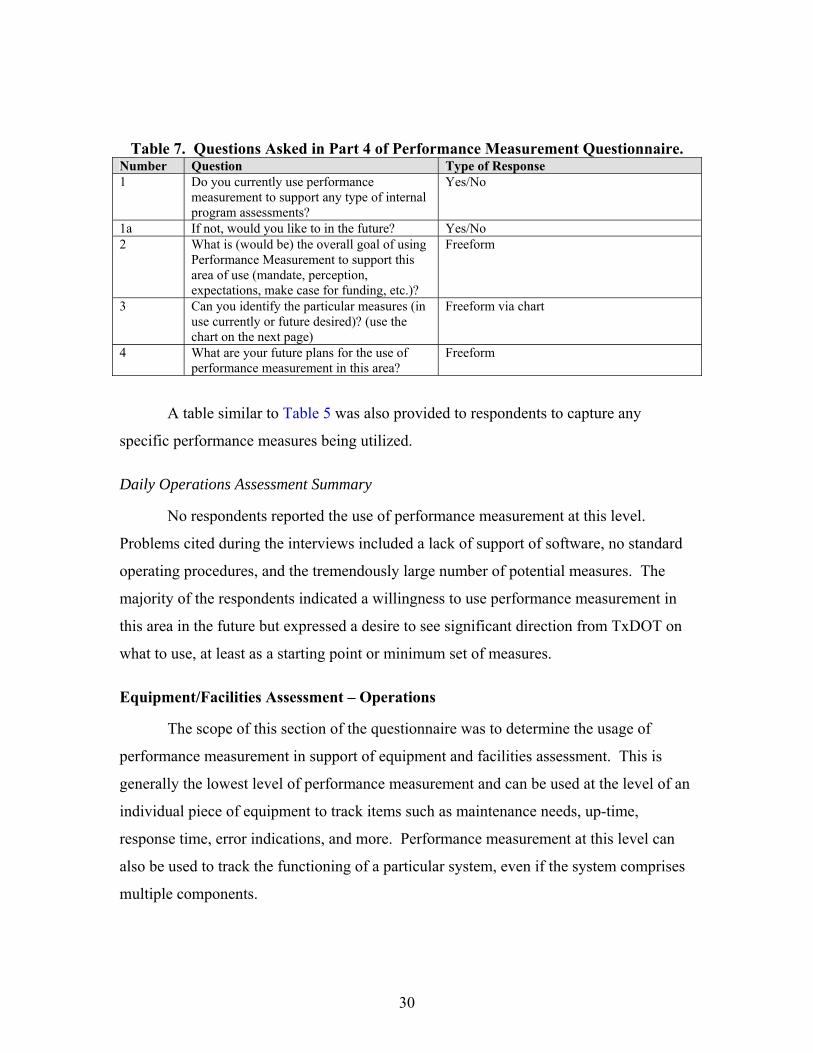
30
Table 7. Questions Asked in Part 4 of Performance Measurement Questionnaire. Number Question Type of Response 1 Do you currently use performance
measurement to support any type of internal program assessments?
Yes/No
1a If not, would you like to in the future? Yes/No 2 What is (would be) the overall goal of using
Performance Measurement to support this area of use (mandate, perception, expectations, make case for funding, etc.)?
Freeform
3 Can you identify the particular measures (in use currently or future desired)? (use the chart on the next page)
Freeform via chart
4 What are your future plans for the use of performance measurement in this area?
Freeform
A table similar to Table 5 was also provided to respondents to capture any
specific performance measures being utilized.
Daily Operations Assessment Summary
No respondents reported the use of performance measurement at this level.
Problems cited during the interviews included a lack of support of software, no standard
operating procedures, and the tremendously large number of potential measures. The
majority of the respondents indicated a willingness to use performance measurement in
this area in the future but expressed a desire to see significant direction from TxDOT on
what to use, at least as a starting point or minimum set of measures.
Equipment/Facilities Assessment – Operations
The scope of this section of the questionnaire was to determine the usage of
performance measurement in support of equipment and facilities assessment. This is
generally the lowest level of performance measurement and can be used at the level of an
individual piece of equipment to track items such as maintenance needs, up-time,
response time, error indications, and more. Performance measurement at this level can
also be used to track the functioning of a particular system, even if the system comprises
multiple components.
RESUBMITTAL
31
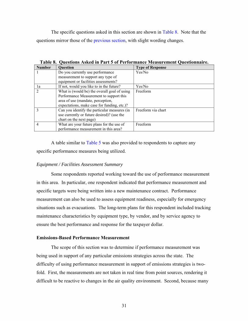
The specific questions asked in this section are shown in Table 8. Note that the
questions mirror those of the previous section, with slight wording changes.
Table 8. Questions Asked in Part 5 of Performance Measurement Questionnaire. Number Question Type of Response 1 Do you currently use performance
measurement to support any type of equipment or facilities assessments?
Yes/No
1a If not, would you like to in the future? Yes/No 2 What is (would be) the overall goal of using
Performance Measurement to support this area of use (mandate, perception, expectations, make case for funding, etc.)?
Freeform
3 Can you identify the particular measures (in use currently or future desired)? (use the chart on the next page)
Freeform via chart
4 What are your future plans for the use of performance measurement in this area?
Freeform
A table similar to Table 5 was also provided to respondents to capture any
specific performance measures being utilized.
Equipment / Facilities Assessment Summary
Some respondents reported working toward the use of performance measurement
in this area. In particular, one respondent indicated that performance measurement and
specific targets were being written into a new maintenance contract. Performance
measurement can also be used to assess equipment readiness, especially for emergency
situations such as evacuations. The long-term plans for this respondent included tracking
maintenance characteristics by equipment type, by vendor, and by service agency to
ensure the best performance and response for the taxpayer dollar.
Emissions-Based Performance Measurement
The scope of this section was to determine if performance measurement was
being used in support of any particular emissions strategies across the state. The
difficulty of using performance measurement in support of emissions strategies is two-
fold. First, the measurements are not taken in real time from point sources, rendering it
difficult to be reactive to changes in the air quality environment. Second, because many
RESUBMITTAL
32
areas in addition to transportation contribute to air quality, assessing the impact of
specifically transportation and crafting strategies to reduce those impacts is also quite
difficult.
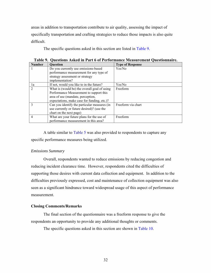
The specific questions asked in this section are listed in Table 9.
Table 9. Questions Asked in Part 6 of Performance Measurement Questionnaire. Number Question Type of Response 1 Do you currently use emissions-based
performance measurement for any type of strategy assessment or strategy implementation?
Yes/No
1a If not, would you like to in the future? Yes/No 2 What is (would be) the overall goal of using
Performance Measurement to support this area of use (mandate, perception, expectations, make case for funding, etc.)?
Freeform
3 Can you identify the particular measures (in use currently or future desired)? (use the chart on the next page)
Freeform via chart
4 What are your future plans for the use of performance measurement in this area?
Freeform
A table similar to Table 5 was also provided to respondents to capture any
specific performance measures being utilized.
Emissions Summary
Overall, respondents wanted to reduce emissions by reducing congestion and
reducing incident clearance time. However, respondents cited the difficulties of
supporting those desires with current data collection and equipment. In addition to the
difficulties previously expressed, cost and maintenance of collection equipment was also
seen as a significant hindrance toward widespread usage of this aspect of performance
measurement.
Closing Comments/Remarks
The final section of the questionnaire was a freeform response to give the
respondents an opportunity to provide any additional thoughts or comments.
The specific questions asked in this section are shown in Table 10.
RESUBMITTAL
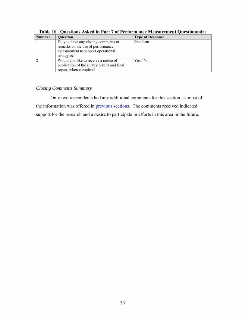
33
Table 10. Questions Asked in Part 7 of Performance Measurement Questionnaire Number Question Type of Response 1 Do you have any closing comments or
remarks on the use of performance measurement to support operational strategies?
Freeform
2 Would you like to receive a notice of publication of the survey results and final report, when complete?
Yes / No
Closing Comments Summary
Only two respondents had any additional comments for this section, as most of
the information was offered in previous sections. The comments received indicated
support for the research and a desire to participate in efforts in this area in the future.
RESUBMITTAL

RESUBMITTAL
35
IMPLEMENTING PERFORMANCE MEASUREMENT
PERFORMANCE MEASURES IN DAILY OPERATIONS
As stated in the introduction, the overall goal of this research project is to
construct a framework that can quantitatively analyze an implemented response and
provide inputs into an assessment methodology to determine the best response. This puts
the focus squarely on daily operations as the appropriate level for this framework to be
developed.
The questionnaire clearly showed that across the state, while performance
measurement is understood and appreciated for what it could provide to transportation
operations, implementation to date is minimal. This was especially true in the arena of
daily operations, as there were no respondents utilizing performance measurement.
One of the critical inputs for effective use is choosing what measures should be
used. This is a significant challenge for daily operations, as literally thousands of
measures could be identified to represent a particular emphasis or strategy or capture a
particular response. It is impossible, however, to implement all of the measures without
creating an incomprehensible system of data collection, storage, and analysis techniques.
What is therefore required is a minimal but comprehensive set of measures that can be
used in daily operations to effectively analyze actions and respond appropriately to
changes. A literature review was performed to determine what lists of measures have
been used external to TxDOT and if there are recommended measures for daily
operations.
TYPES OF PERFORMANCE MEASUREMENT
Input/Output/Outcome
Performance measures may be classified in any number of ways. One of the
simplest methods of classification is to identify each measure as an input, output, or
outcome.
An input measure examines the resources available to carry out a program. The
selection of the performance measure may be difficult to evaluate if the input parameter
RESUBMITTAL
36
is difficult to obtain. One example might be the number of vehicles that enter a corridor
that is supported by a Traffic Management Center
An output value is usually a quantitative value that is based on a tabulation
calculation or measurement. One example of an output performance measure is the travel
time through a corridor or segment of highway.
An outcome variable is usually more subjective. An outcome performance
measure provides an assessment of the results of a traffic management tool or strategy or
institutional program. The outcome answers the effectiveness of the current program.
In many cases, a performance measurement system may use measures from all
three areas. One example is the effectiveness of the number of incident management
response teams on the amount of clearance time along Interstate 10. In this example the
input is the number of response teams and the output is the average time to clear an
incident along I-10. The output may be that the increase in incident response teams
improved the incident clearance time by 10 percent, saving the motorists more than one
million dollars per year. As a result of the input and the output, this theoretical case
would be considered an effective institutional policy for improving incident clearance
times.
Goal-Based Classification
Performance measures may also be evaluated based on the goals of the program.
Identifying the goals helps to provide a continual focus for the agency of the TMC. In
this classification system, the performance measure should help to determine the progress
of the program in relationship to the overall goals and/or objectives of the system. Some
goals commonly used in this type of performance measure classification include:
• Accessibility – ensuring convenience and or right-of-entry to customers;
• Mobility – relative ease of difficulty of making a trip;
• Economic Development – cost, economic health, and vitality of the
transportation system;
• Quality of Life – sense of community desires and customer satisfaction;
• Environmental and Resource Conservation – assets saved or expended,
wither natural or man-made;
RESUBMITTAL
37
• Safety – levels and rates of incidents or other occurrences;
• Operational Efficiency – productivity, manpower, financial resources, etc;
and
• System Condition and Performance – physical conditions, service ranges,
etc.
It is not uncommon for a goal-based system to use a secondary classification
scheme. Mobility, for example, may be divided into passenger or freight mobility. Safety
may be divided into roadway, rail, transit, parking, pedestrian, freight, and more. In some
cases, the secondary classification does not need to be consistent with the overall
framework of the program. The secondary classification may provide information across
multiple performance measures and in some cases, the secondary classification may have
a greater impact on one of the performance measures. One example of this last case may
be the impact of vehicle speed. In one case vehicle speeds are very fast and travel time
and overall mobility is efficient. However, under this theoretical example the number of
crashes increases exponentially and lowers the safety of the corridor. In this case the
final goal of secondary classification needs to be analyzed or weighted by the local staff.
CHALLENGES OF PERFORMANCE MEASURES
The results of the literature reviews, the TxDOT questionnaire, knowledge of
ATMS software, and casual observation of web sites clearly indicate that the majority of
agencies are still using the most basic performance measures to describe freeway
operations.
One potential reason is that assessing operational performance is still a relatively
new area. Data needs for calculating measures beyond the basics may not be supported
by existing infrastructure and ATMS programs. Because the use of supplementary
measures may involve additional data collection or software development, significant
cost may be involved in migrating toward more sophisticated measures.
A second potential reason why basic measures are used is that the variety of
available performance measures is large. As an example, consider the measurement of
congestion. Performance measures related to congestion may be based upon :
RESUBMITTAL
38
• Duration – focus on the temporal limits of the congestion,
• Extent – focus on the geographic limits of congestion,
• Intensity – focus on the severity of the congestion, or
• Reliability – focus on the variation in the congestion (2).
The number of different measures that could be used to describe a single concept
(such as density) may be very confusing to different audiences, perhaps most especially
to the traveling public. The need to communicate exactly what the measures describe is
an impediment to their wide-scale acceptance and use.
A third potential reason why more sophisticated measures are not used may be the
data necessary to support their use. Many of these more sophisticated measures require a
baseline—a point of comparison for understanding normal conditions. This comparison
requires collection, storage, and availability of roadway data for comparison use.
Consider the use of speed as a performance measure. It is generally well
understood and because it provides an indication of the system at a specific location and
point in time, it requires no reference point. In comparison, consider the use of queue
length after an incident. In order to be effective, this performance measure has to be
examined over time. Is the queue length decreasing or increasing? How far back from
the incident does the queue start? Analyzing these performance measures may provide a
more detailed understanding of an incident and the operational response necessary to
clear it from the roadway, but it requires a baseline in time and space that translates to
extensive data needs.
The archival of data to support this need is not an insignificant task. The roadway
infrastructure generates a tremendous volume of data. As an example, consider that the
26-mile phase one deployment in San Antonio, Texas, generated nearly one gigabyte of
raw data per day (14). While that amount is not as difficult to deal with as it was even
five years ago, expanding the coverage area to three or four times the of phase one
deployment and keeping the data for a year would result in the need for more than a
terabyte of space. That amount of data storage can be costly and is certainly not a trivial
matter to incorporate into an archive data library. Also, the time required to process and
perform calculations using that much data must be considered in any system design.
RESUBMITTAL
39
As operational performance measurement becomes more commonplace, programs
will begin to employ a broad spectrum of measures to capture all of the various facets of
program use. NCHRP 446 (19) discusses the differentiation of output and outcome
performance measures. Output measures are indicators of resources utilized or perhaps
the scope of activities performed. Output measures identify information about the
management of resources and are most useful in a performance-based system. In
contrast, outcome measures are often more indicative of how well an agency meets its
goals and objectives. Outcome-based measures are more likely to be significant and
understandable to the general public. However, both types of measures are useful, and a
successful performance measurement system generally includes both.
Consider, for example, an area of concern related to safety in icy conditions. An
output measure might be the number of tons of salt applied to the roadway. While this
measure has a majority of the 10 characteristics listed above and is easily understood and
measured, it is most applicable to the agency in charge of the roadways. The
corresponding outcome measure might be the number of ice-related accidents. This
measure is much more easily understood by the traveling public and can be shown over
time and large areas to highlight improvements to the system. Both types of measures
work in conjunction with one another to provide a complete analysis and evaluation of
the system (19).
In addition to looking at the factors discussed above, determination of the
appropriate performance measures also requires consideration of other aspects of the
system. One important consideration is who will be using the measures. A number of
different types of activities take place in a transportation environment, from planning and
design to operations and maintenance. Careful consideration of each of these specific
needs creates a stronger success potential for a performance measurement system.
Performance measurement systems should also consider users beyond the general public.
These can include elected officials, the media, and users in the judicial system, to name a
few (20).
Another consideration is the increasing assessment of the multi-modality of
transportation systems. As such, measures that concentrate on the mobility of the entire
system, rather than a specific node, may prove to be very useful and necessary. Mode-
RESUBMITTAL
40
specific measures may be used in conjunction with the multi-modal approach to identify
any deficiencies and to determine individual mode effects.
What Makes A Good Measure?
First and foremost, a performance measure must measure or gauge the right item.
It does so by focusing on the goals and objectives and determining if they are being met.
A performance measure should focus on the end result—not the measurement itself.
The second trait of a good performance measure is that it is accepted. Generally,
this means that the measure must be simple, understandable, unambiguous, and
meaningful to the customer, regardless of who the customer is. To best accomplish this,
agencies may use different measures for different customers.
The third trait is that performance measures must be responsive and/or sensitive to
the data they measure. They do this by clearly showing trends, changes, minimums, or
maximums. A performance measure that is insensitive to these events within the data
will not be meaningful to the customer because it cannot accurately depict progress
toward the system goals.
The fourth trait of a good measure is that it is appropriate. Judging the
appropriateness of a selection is typically done in two ways. First, the measure must be
temporally appropriate. If the desire is to determine a percent reduction in incidents, the
measure should look at a lengthy analysis period, such as a week, a month, or even a
year. Reporting on a time frame of minutes, hours, or even a day would make little sense
and would be an inappropriate time frame for this measure. Second, the measure must be
geographically appropriate. Measures can be directed toward a point, a segment, an
entire facility or travel corridor, or even a region. A reduction in travel time would not
make sense at a point location but might be a good measure from a corridor or regional
perspective.
A fifth and somewhat arguable trait is that a good performance measure should be
supportable by economical data collection. Measures that require large and expensive
data collection are not likely to be determined very often, due to time and/or budgetary
constraints. This makes the measure untimely and insensitive to smaller changes, and
ultimately it will not convey meaningful results. At the same time, TMCs should
RESUBMITTAL
41
recognize that it is OK to stretch beyond the current practice and find and collect
additional data sources, if the performance measures can provide meaningful results.
This trait is arguable because many agencies have fallen into the trap of only looking at
measures that can be supported by data they already collect. This can hinder effective
evaluations and often results in choosing measures that do not support the stated goals.
Keys to a Successful Program
Over time, researchers have identified a number of keys to having a successful
performance management program. These keys, listed below, are not set in stone but
provide some guiding principles to help organizations navigate through the chore of
picking appropriate measures. These keys are not an exhaustive list from the literature
but rather a compilation of those items and advice which are commonly accepted and
indisputable.
• Keep the number of measures manageable – Include measures when
significant, but exclude measures that are merely interesting and not directly
relevant.
• Use a balance of measures – Provide both output and outcome measures.
Determine the critical areas of focus in your TMC and select measures for
each area. Remember that some measures are more suited to a particular
audience and ensure that the selection of measures can adequately convey
understanding to each group of stakeholders.
• Be flexible – TMCs, especially new ones, should experiment with
performance measures in order to find the right mix and set that capture and
support the specific operating environment.
• Go beyond the basics – While it is recognized that simplicity and ease of
measurement are attractive characteristics, especially to a new TMC, an
agency should not shy away from areas that are hard to quantify or where
data may be difficult to obtain. This pushes a TMC to grow and increase its
capabilities and ultimately provide a better service to the stakeholders.
• Establish regular reviews – The performance measurement process should
recognize the need for regular review. While the framework provides
RESUBMITTAL
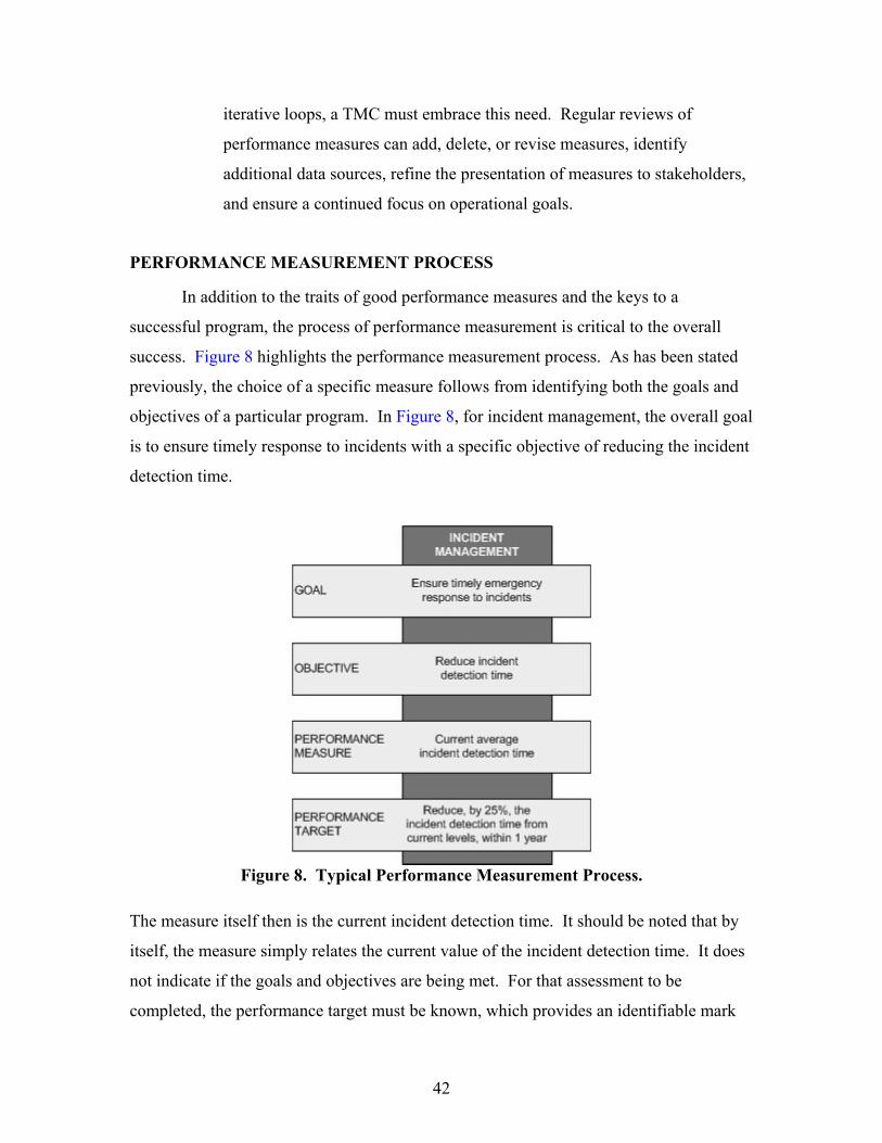
42
iterative loops, a TMC must embrace this need. Regular reviews of
performance measures can add, delete, or revise measures, identify
additional data sources, refine the presentation of measures to stakeholders,
and ensure a continued focus on operational goals.
PERFORMANCE MEASUREMENT PROCESS
In addition to the traits of good performance measures and the keys to a
successful program, the process of performance measurement is critical to the overall
success. Figure 8 highlights the performance measurement process. As has been stated
previously, the choice of a specific measure follows from identifying both the goals and
objectives of a particular program. In Figure 8, for incident management, the overall goal
is to ensure timely response to incidents with a specific objective of reducing the incident
detection time.
Figure 8. Typical Performance Measurement Process.
The measure itself then is the current incident detection time. It should be noted that by
itself, the measure simply relates the current value of the incident detection time. It does
not indicate if the goals and objectives are being met. For that assessment to be
completed, the performance target must be known, which provides an identifiable mark
RESUBMITTAL

43
with a time frame. These parameters can then be used to judge the effectiveness of the
incident detection mechanism in an incident management program.
RESUBMITTAL

RESUBMITTAL
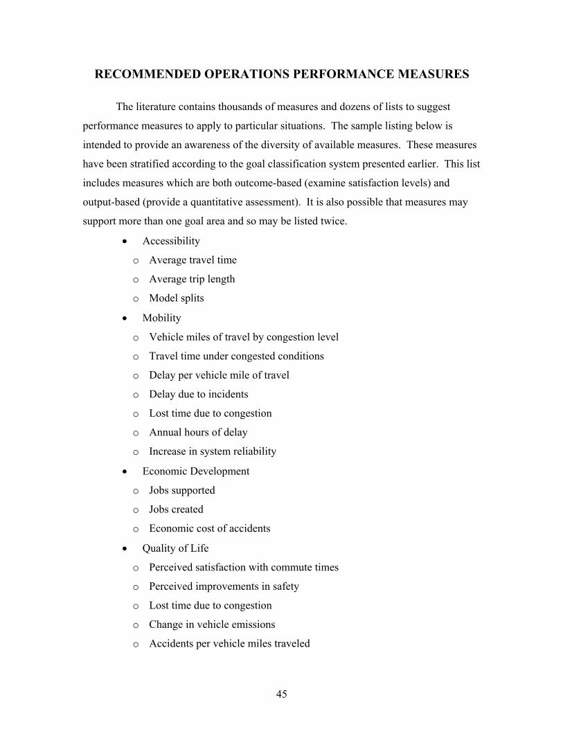
45
RECOMMENDED OPERATIONS PERFORMANCE MEASURES
The literature contains thousands of measures and dozens of lists to suggest
performance measures to apply to particular situations. The sample listing below is
intended to provide an awareness of the diversity of available measures. These measures
have been stratified according to the goal classification system presented earlier. This list
includes measures which are both outcome-based (examine satisfaction levels) and
output-based (provide a quantitative assessment). It is also possible that measures may
support more than one goal area and so may be listed twice.
• Accessibility
o Average travel time
o Average trip length
o Model splits
• Mobility
o Vehicle miles of travel by congestion level
o Travel time under congested conditions
o Delay per vehicle mile of travel
o Delay due to incidents
o Lost time due to congestion
o Annual hours of delay
o Increase in system reliability
• Economic Development
o Jobs supported
o Jobs created
o Economic cost of accidents
• Quality of Life
o Perceived satisfaction with commute times
o Perceived improvements in safety
o Lost time due to congestion
o Change in vehicle emissions
o Accidents per vehicle miles traveled
RESUBMITTAL
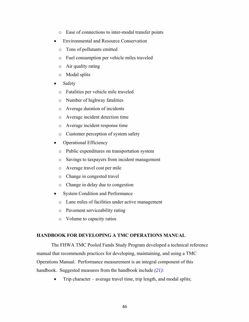
46
o Ease of connections to inter-modal transfer points
• Environmental and Resource Conservation
o Tons of pollutants emitted
o Fuel consumption per vehicle miles traveled
o Air quality rating
o Modal splits
• Safety
o Fatalities per vehicle mile traveled
o Number of highway fatalities
o Average duration of incidents
o Average incident detection time
o Average incident response time
o Customer perception of system safety
• Operational Efficiency
o Public expenditures on transportation system
o Savings to taxpayers from incident management
o Average travel cost per mile
o Change in congested travel
o Change in delay due to congestion
• System Condition and Performance
o Lane miles of facilities under active management
o Pavement serviceability rating
o Volume to capacity ratios
HANDBOOK FOR DEVELOPING A TMC OPERATIONS MANUAL
The FHWA TMC Pooled Funds Study Program developed a technical reference
manual that recommends practices for developing, maintaining, and using a TMC
Operations Manual. Performance measurement is an integral component of this
handbook. Suggested measures from the handbook include (21):
• Trip character – average travel time, trip length, and modal splits;
RESUBMITTAL
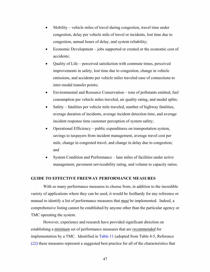
47
• Mobility – vehicle miles of travel during congestion, travel time under
congestion, delay per vehicle mile of travel or incidents, lost time due to
congestion, annual hours of delay, and system reliability;
• Economic Development – jobs supported or created or the economic cost of
accidents;
• Quality of Life – perceived satisfaction with commute times, perceived
improvements in safety, lost time due to congestion, change in vehicle
emissions, and accidents per vehicle miles traveled ease of connections to
inter-modal transfer points;
• Environmental and Resource Conservation – tons of pollutants emitted, fuel
consumption per vehicle miles traveled, air quality rating, and modal splits;
• Safety – fatalities per vehicle mile traveled, number of highway fatalities,
average duration of incidents, average incident detection time, and average
incident response time customer perception of system safety;
• Operational Efficiency – public expenditures on transportation system,
savings to taxpayers from incident management, average travel cost per
mile, change in congested travel, and change in delay due to congestion;
and
• System Condition and Performance – lane miles of facilities under active
management, pavement serviceability rating, and volume to capacity ratios.
GUIDE TO EFFECTIVE FREEWAY PERFORMANCE MEASURES
With so many performance measures to choose from, in addition to the incredible
variety of applications where they can be used, it would be foolhardy for any reference or
manual to identify a list of performance measures that must be implemented. Indeed, a
comprehensive listing cannot be established by anyone other than the particular agency or
TMC operating the system.
However, experience and research have provided significant direction on
establishing a minimum set of performance measures that are recommended for
implementation by a TMC. Identified in Table 11 (adopted from Table 4-5, Reference
(22) these measures represent a suggested best practice for all of the characteristics that
RESUBMITTAL
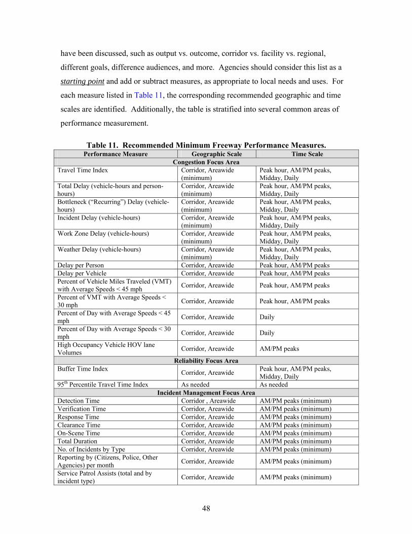
48
have been discussed, such as output vs. outcome, corridor vs. facility vs. regional,
different goals, difference audiences, and more. Agencies should consider this list as a
starting point and add or subtract measures, as appropriate to local needs and uses. For
each measure listed in Table 11, the corresponding recommended geographic and time
scales are identified. Additionally, the table is stratified into several common areas of
performance measurement.
Table 11. Recommended Minimum Freeway Performance Measures. Performance Measure Geographic Scale Time Scale
Congestion Focus Area Travel Time Index Corridor, Areawide
(minimum) Peak hour, AM/PM peaks, Midday, Daily
Total Delay (vehicle-hours and person-hours)
Corridor, Areawide (minimum)
Peak hour, AM/PM peaks, Midday, Daily
Bottleneck (“Recurring”) Delay (vehicle-hours)
Corridor, Areawide (minimum)
Peak hour, AM/PM peaks, Midday, Daily
Incident Delay (vehicle-hours) Corridor, Areawide (minimum)
Peak hour, AM/PM peaks, Midday, Daily
Work Zone Delay (vehicle-hours) Corridor, Areawide (minimum)
Peak hour, AM/PM peaks, Midday, Daily
Weather Delay (vehicle-hours) Corridor, Areawide (minimum)
Peak hour, AM/PM peaks, Midday, Daily
Delay per Person Corridor, Areawide Peak hour, AM/PM peaks Delay per Vehicle Corridor, Areawide Peak hour, AM/PM peaks Percent of Vehicle Miles Traveled (VMT) with Average Speeds < 45 mph Corridor, Areawide Peak hour, AM/PM peaks
Percent of VMT with Average Speeds < 30 mph Corridor, Areawide Peak hour, AM/PM peaks
Percent of Day with Average Speeds < 45 mph Corridor, Areawide Daily
Percent of Day with Average Speeds < 30 mph Corridor, Areawide Daily
High Occupancy Vehicle HOV lane Volumes Corridor, Areawide AM/PM peaks
Reliability Focus Area Buffer Time Index Corridor, Areawide Peak hour, AM/PM peaks,
Midday, Daily 95th Percentile Travel Time Index As needed As needed
Incident Management Focus Area Detection Time Corridor , Areawide AM/PM peaks (minimum) Verification Time Corridor, Areawide AM/PM peaks (minimum) Response Time Corridor, Areawide AM/PM peaks (minimum) Clearance Time Corridor, Areawide AM/PM peaks (minimum) On-Scene Time Corridor, Areawide AM/PM peaks (minimum) Total Duration Corridor, Areawide AM/PM peaks (minimum) No. of Incidents by Type Corridor, Areawide AM/PM peaks (minimum) Reporting by (Citizens, Police, Other Agencies) per month Corridor, Areawide AM/PM peaks (minimum)
Service Patrol Assists (total and by incident type) Corridor, Areawide AM/PM peaks (minimum)
RESUBMITTAL
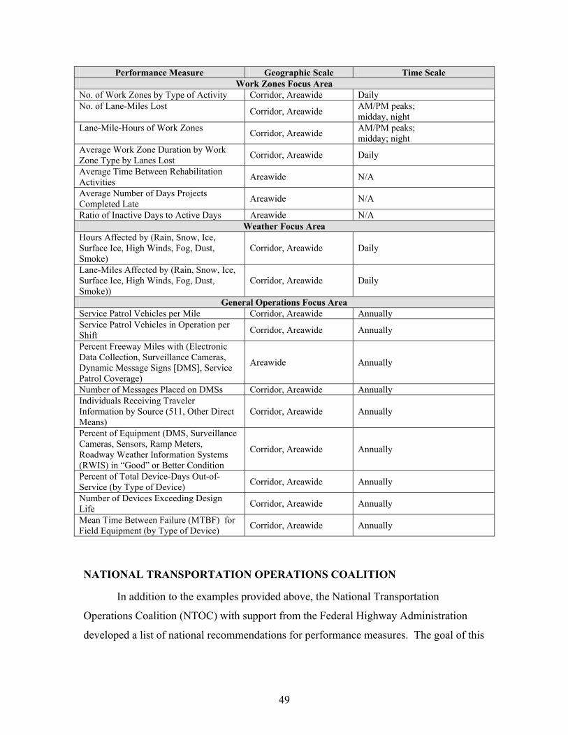
49
Performance Measure Geographic Scale Time Scale Work Zones Focus Area
No. of Work Zones by Type of Activity Corridor, Areawide Daily No. of Lane-Miles Lost Corridor, Areawide AM/PM peaks;
midday, night Lane-Mile-Hours of Work Zones Corridor, Areawide AM/PM peaks;
midday; night Average Work Zone Duration by Work Zone Type by Lanes Lost Corridor, Areawide Daily
Average Time Between Rehabilitation Activities Areawide N/A
Average Number of Days Projects Completed Late Areawide N/A
Ratio of Inactive Days to Active Days Areawide N/A Weather Focus Area
Hours Affected by (Rain, Snow, Ice, Surface Ice, High Winds, Fog, Dust, Smoke)
Corridor, Areawide Daily
Lane-Miles Affected by (Rain, Snow, Ice, Surface Ice, High Winds, Fog, Dust, Smoke))
Corridor, Areawide Daily
General Operations Focus Area Service Patrol Vehicles per Mile Corridor, Areawide Annually Service Patrol Vehicles in Operation per Shift Corridor, Areawide Annually
Percent Freeway Miles with (Electronic Data Collection, Surveillance Cameras, Dynamic Message Signs [DMS], Service Patrol Coverage)
Areawide Annually
Number of Messages Placed on DMSs Corridor, Areawide Annually Individuals Receiving Traveler Information by Source (511, Other Direct Means)
Corridor, Areawide Annually
Percent of Equipment (DMS, Surveillance Cameras, Sensors, Ramp Meters, Roadway Weather Information Systems (RWIS) in “Good” or Better Condition
Corridor, Areawide Annually
Percent of Total Device-Days Out-of-Service (by Type of Device) Corridor, Areawide Annually
Number of Devices Exceeding Design Life Corridor, Areawide Annually
Mean Time Between Failure (MTBF) for Field Equipment (by Type of Device) Corridor, Areawide Annually
NATIONAL TRANSPORTATION OPERATIONS COALITION
In addition to the examples provided above, the National Transportation
Operations Coalition (NTOC) with support from the Federal Highway Administration
developed a list of national recommendations for performance measures. The goal of this
RESUBMITTAL
50
list was to define approximately 10 measures commonly agreed upon by federal, state,
and local transportation officials (NTOC). NTOC includes representatives from:
• America Association of State Highway and Transportation Officials
(AASHTO),
• International City/County Management Association (ICMA),
• Transportation Research Board (TRB) ,
• Association of Metropolitan Planning Organizations (AMPO),
• American Public Works Association (APWA), and
• Institute of Transportation Engineers (ITE) (23).
These national recommendations were developed to help local traffic
administrators with the selection of performance measures and to encourage more
national uniformity. The goal of these performance measures is to be used for internal
management, external communications, and comparative measurements (23).
The results from NTOC include the following suggestions of performance
measures:
• customer satisfaction,
• extent of congestion – spatial,
• extent of congestion – temporal,
• incident duration,
• non-recurring delay,
• recurring delay,
• speed,
• throughput – person,
• throughput – vehicle,
• travel time – link,
• travel time – reliability, and
• travel time – trip.
Customer Satisfaction
Customer satisfaction is a qualitative measure based on the opinions of the
motorist. Customer satisfaction includes operations on freeway, arterial, corridors, and
RESUBMITTAL
51
regions. In most cases, customer satisfaction does not include surveys (23). Some
common questions to determine customer satisfaction include:
• How long was your commute to work?
• Are you satisfied with the amount of time required for local traffic activity?
• Did the TMC provide you with adequate information about the roadway?
• Are you satisfied with the various sources of information?
In most cases, the motorists’ opinions are rated as very satisfied, somewhat
satisfied, neutral, somewhat dissatisfied, very dissatisfied, and don’t know or not
applicable.
Extent of Congestion – Spatial
The extent of spatial congestion is defined by how widespread the congestion is.
This performance is defined by the local agencies’ definition of congestion. NTOC
defines congestion as periods where travel time is 30 percent longer than unconstrained
travel times. This performance measure is usually quantitative and may be defined as the
number of centerline miles with congested conditions. This performance measure may
also be defined on a regional or corridor level by the percentage of centerline miles that
are under congestion versus the number of total miles in the region of the corridor. The
calculation of this performance measure may also be defined by the time of day.
Extent of Congestion – Temporal
The temporal extent of congestion is the second performance measure that may be
used to evaluate the congestion associated with a link, corridor, or region. This
performance measure is quantitative and may be used in association with the spatial
extent of congestion. The temporal performance measure is the time duration in which
20 percent of the roadway sections in the area of question are considered under congested
by the spatial congestion definition.
Incident Duration
The incident duration is the amount of time elapsed from the notification of the
incident until the incident has been removed or the service/response vehicles have left the
incident. This measure is quantitative and may be defined as the amount of time elapsed
RESUBMITTAL
52
between the notification of an incident and the amount of time for the complete clearing
or removal of the incident. This measure may be applied to safety patrols, emergency
response programs, and tow companies.
Non-Recurring Delay
Non-recurring delay is the number of vehicle hours that are associated with delays
in excess of common recurring delays. Non-recurring delays may include holidays, the
impacts of work zone construction periods, or intersections of two highway interchanges,
etc.
Recurring Delay
Recurring delays are vehicle delays that are repeatable for the current time-of-day,
day-of-week, and day-type. Congestion associated with recurring delay is defined by the
travel time actually required to traverse the corridor and the unconstrained travel time.
Common examples of recurring delay are morning and afternoon rush hours or the
amount of time associated with a signal corridor.
Speed
The speed performance measure is the average point mean speed for vehicles
traveling on an individual lane in one direction. The speed performance measure is
typically used for various types of recurring and non-recurring congestion and
unconstrained travel.
Throughput – Person
The throughput person performance measure is the number of people that travel
across a segment of roadway over a given time. The typical unit for measurement is the
number of persons per hour. This value includes vehicle occupants, pedestrians, and
bicyclists. This performance measure is usually used to evaluate person-carrying
capacity for planning and operations purposes.
RESUBMITTAL
53
Throughput – Vehicle
The throughput vehicle performance measure is the number of vehicles that travel
across a segment of roadway for a particular time period. The throughput vehicle
performance measure is in units of vehicles per hour. Similar to the previous
performance measure, the vehicle throughput is calculated for recurring and non-
recurring congestion as well as unconstrained flow.
Travel Time – Link
The travel time link performance measure is the amount of time required for one
vehicle to travel in one single direction across a link. This performance measure includes
vehicles on all roadway types that are traveling through recurring, non-recurring, and
unconstrained flow. A link is typically a section of freeway between intersections or a
segment between traffic signals or it may be defined by local agencies or municipalities.
The units of measurement are the number of minutes per trip. The link-based travel time
performance measure is used by planning and operations agencies (23). Link-based
travel time may be used for evaluating flow through work zones, improvements in single
timing, or increased capacity along a roadway.
Travel Time – Reliability
Travel time reliability is the amount of additional time required by a motorist to
reach the intended location within an allotted time over 95 percent of trips. Travel time
reliability may be calculated for all types of roadways for all travel conditions. This
measure is intended to be applied to a specific time of the day during which repeatable
traffic and roadway conditions typically exist.
Travel Time – Trip
The travel time trip performance measurement is the average time required to
travel from the origin to the destination and may be calculated for multiple modes of
travel. This type of information is useful for traveler information and outreach.
Examples might include the amount of time that it takes a motorist to travel through a
work zone, travel to the airport, or travel the incoming/outgoing direction during a
commuting period..
RESUBMITTAL

54
SUMMARY OF RECOMMENDED MEASURES
Despite the literature review and the sample listings above, there exists no
definitive listing of recommended performance measures for the analysis of daily
operations. As is evident, most of the measures in the literature focus on the higher levels
of system analysis, such as system-wide or inter-agency operations. Throughout the
second year of the project, the research team will be working to construct a recommended
basic list that incorporates the principles of good performance measurement detailed
above, as well as being specific enough to effectively analyze operations.
RESUBMITTAL
55
RECOMMENDED EMISSIONS PERFORMANCE MEASURES
EVALUATING THE PERFORMANCE OF AMBIENT AIR QUALITY
Natural phenomena and humans primarily cause air pollution. Reducing air
pollution from natural sources is difficult, while reducing air pollution from human
activities is relatively easier, especially in the transportation sector, which generates high
levels of carbon monoxide (CO), hydrocarbons (HC), and nitrogen oxides (NOx).
All air pollution, natural or human-made, can affect humans, animals, vegetation,
materials, and structures, where the impact depends on the type of pollutant and exposure
time. For example, an acute impact of coarse particulate matter (PM10) concentration
above 500 μg/m3 can lead to human death within 24 hours, whereas the same effect may
occur when ozone (O3) concentration exceeds 1000 μg/m3 for a one-hour exposure time.
Some pollutants such as fine particulates (PM2.5) also impact human health in the long
term and lead to chronic disease (24). Air pollution impacts can be divided into three
levels: global, regional, and local. At the global level, carbon dioxide (CO2) can increase
global temperature, which leads to an increase in sea level and global warming. At the
regional level, air pollution impacts can transfer from one region to another by wind. At
the local level, the air pollution impacts occur in a particular area, such as county or city.
To assess any effects on ambient air quality, emissions’ impact on humans,
animals, vegetation, materials, and structures must be well understood. Thus, the first
section presents the impacts of air pollution on human health, focusing on the six criteria
air pollutants, carbon monoxide (CO), particulate matter (PM), nitrogen dioxide (NO2),
lead (Pb), sulfur dioxide (SO2), and ozone (O3) designated by the U.S. Environmental
Protection Agency (EPA). The second section describes the National Ambient Air
Quality Standards (NAAQS) and other countries’ air pollution standards, as well as the
application of air pollution indices. The third section addresses air pollution monitoring
and measurement. Finally, the fourth section reviews the emission performance measures
used in the United States and recommends performance measurement strategies to
evaluate changes in emissions from the freeway system.
RESUBMITTAL
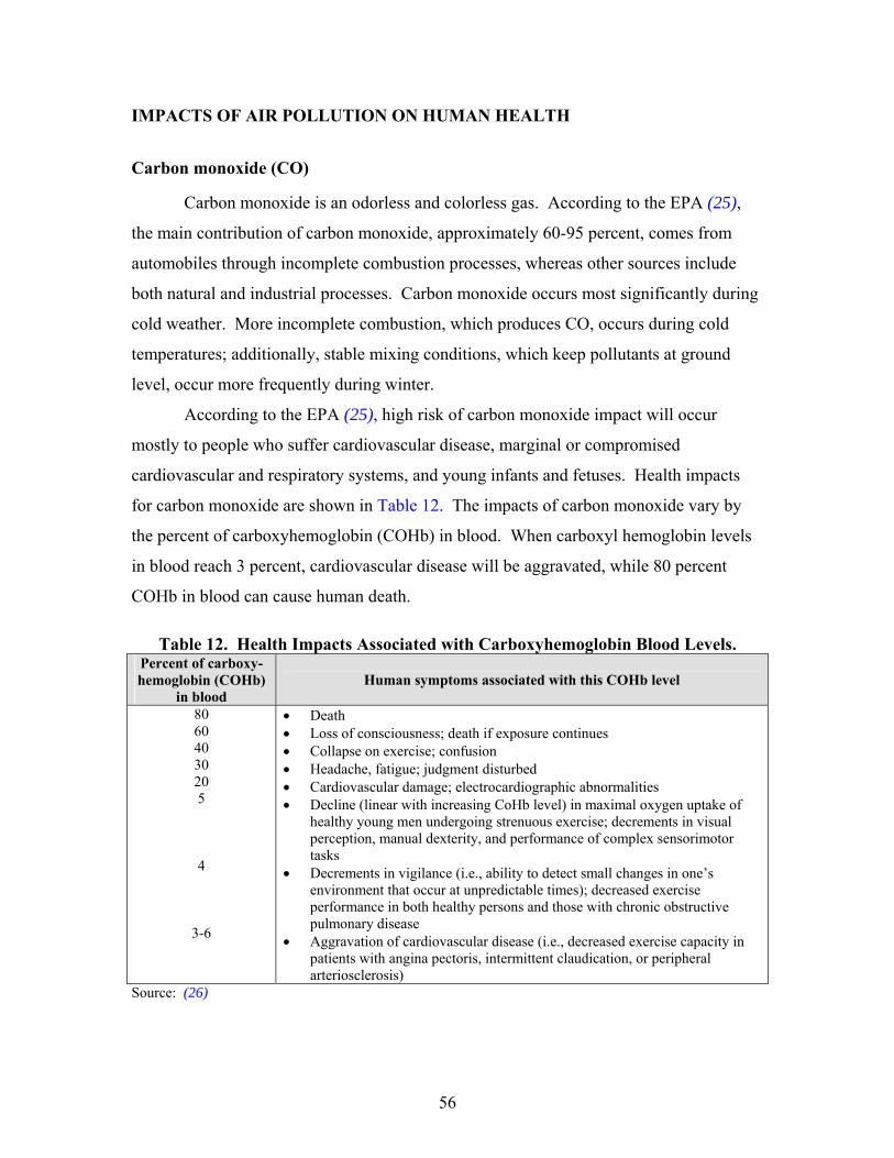
56
IMPACTS OF AIR POLLUTION ON HUMAN HEALTH
Carbon monoxide (CO)
Carbon monoxide is an odorless and colorless gas. According to the EPA (25),
the main contribution of carbon monoxide, approximately 60-95 percent, comes from
automobiles through incomplete combustion processes, whereas other sources include
both natural and industrial processes. Carbon monoxide occurs most significantly during
cold weather. More incomplete combustion, which produces CO, occurs during cold
temperatures; additionally, stable mixing conditions, which keep pollutants at ground
level, occur more frequently during winter.
According to the EPA (25), high risk of carbon monoxide impact will occur
mostly to people who suffer cardiovascular disease, marginal or compromised
cardiovascular and respiratory systems, and young infants and fetuses. Health impacts
for carbon monoxide are shown in Table 12. The impacts of carbon monoxide vary by
the percent of carboxyhemoglobin (COHb) in blood. When carboxyl hemoglobin levels
in blood reach 3 percent, cardiovascular disease will be aggravated, while 80 percent
COHb in blood can cause human death.
Table 12. Health Impacts Associated with Carboxyhemoglobin Blood Levels. Percent of carboxy- hemoglobin (COHb)
in blood Human symptoms associated with this COHb level
80 60 40 30 20 5
4
3-6
• Death • Loss of consciousness; death if exposure continues • Collapse on exercise; confusion • Headache, fatigue; judgment disturbed • Cardiovascular damage; electrocardiographic abnormalities • Decline (linear with increasing CoHb level) in maximal oxygen uptake of
healthy young men undergoing strenuous exercise; decrements in visual perception, manual dexterity, and performance of complex sensorimotor tasks
• Decrements in vigilance (i.e., ability to detect small changes in one’s environment that occur at unpredictable times); decreased exercise performance in both healthy persons and those with chronic obstructive pulmonary disease
• Aggravation of cardiovascular disease (i.e., decreased exercise capacity in patients with angina pectoris, intermittent claudication, or peripheral arteriosclerosis)
Source: (26)
RESUBMITTAL
57
According to Stern (27), the effects of carbon monoxide depend on how much is
accumulated in the human body. The level of carboxyl hemoglobin can increase with
human exposure to high carbon monoxide levels, leading to a decrease in the capability
of carrying oxygen from the lungs to body tissues. The amount of carbon monoxide in the
human body can be estimated from the amount of carbon monoxide carried by
hemoglobin. The relationship between the ratio of carbon monoxide and oxygen and the
ratio of carboxyhemoglobin and oxyhemoglobin is described by the Haldane equation
below:
)()(
%%
22 O
CO
pp
MHbO
COHb=
Where:
• M is known as the Haldane Constant and is approximately 245
• %COHb and %O2Hb are the amount of hemoglobin combined with carbon
monoxide and oxygen, respectively
• COp and 2Op are the proportion of gas molecules of carbon monoxide and
oxygen in air
The equation can describe the effects of high altitude (low2Op ), carbon monoxide,
and the removal of carbon monoxide from the human body by increasing the oxygen.
However, the equation cannot estimate how much time the process will take, due to the
individual differences in the capability of carrying oxygen to body tissues. In addition,
humans can receive and excrete carbon monoxide from the body. Thus, the impacts of
carbon monoxide on human health are complex and depend on exposure time, carbon
monoxide concentration, and the amount of carbon monoxide remaining in the body after
the processes of absorption and excretion.
Particulate Matter (PM)
According to Sattler (28), particulate matter is any substance except pure water
that exists in the atmosphere in the form of a liquid or solid. Particulates can be emitted
directly from sources, such as vehicles or power plants, or formed via chemical reactions
with other pollutants. Particulates are classified into two groups based on their
dimensions: fine particles and coarse particles. Fine particles, or PM2.5, have a diameter
RESUBMITTAL
58
less than 2.5 micrometers. Sources of PM2.5 include the combustion process in motor
vehicles, power plants, and forest fires. Coarse particles, or PM10, have a diameter
greater than 2.5 micrometers but less than 10 micrometers. PM10 occurs through crushing
or grinding operations or dust being stirred up by vehicles (25).
The main sources of particulate matter are industrial processes. Table 13 shows
that most particulates are generated from industrial processes, and only 20–21 percent of
PM10 is generated by highway and off-highway vehicles. The particulates from different
industries have diverse constituents, such as heavy metals and organic compounds. The
impacts of particulate matter depend on the size of particulate. The smaller sizes of a
particulate (diameter less than 0.5 micrometers) can be transported by wind over a longer
distance than large size particulates. Thus, they will spread widely and have more serious
effects than the larger particulates. According to Cooper and Alley (29), small particle
size causes more severe damage to human health than large particle size. PM2.5 can
penetrate deeply into lungs for longer periods of time, while PM10 can be trapped by
nasal hairs or settle onto the mucous membranes in the nasal or oral passages or trachea.
Insoluble particles can be swallowed or expectorated.
Pope et al. (31) studied the acute effects of particulates by increasing PM10
concentration in 10 μg/m3 intervals. They evaluated data from 10 cities collected over
one to a few days. Health measures including hospital admissions, respiratory and
cardiac symptoms and deaths, and pulmonary function were studied. Factors such as age,
gender, education, income, smoking, and health status were ignored due to the short
period of time. The results of the study indicated that each increasing increment of
10 μg/m3 PM10 concentration led to an increase of human disease of 1-3 percent, while
damaging lung function by 0.1 percent (see Table 14).
RESUBMITTAL
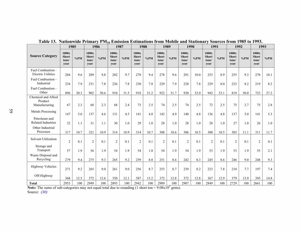
59
Table 13. Nationwide Primary PM10 Emission Estimations from Mobile and Stationary Sources from 1985 to 1993. 1985 1986 1987 1988 1989 1990 1991 1992 1993
Source Category 1000x Short tons/ year
%PM
1000x Short tons/ year
%PM
1000x Short tons/ year
%PM
1000x Short tons/ year
%PM
1000x Short tons/ year
%PM
1000x Short tons/ year
%PM
1000x Short tons/ year
%PM
1000x Short tons/ year
%PM
1000x Short tons/ year
%PM
Fuel Combustion - Electric Utilities 284 9.6 289 9.8 282 9.7 278 9.4 278 9.6 291 10.0 253 8.9 255 9.3 270 10.1
Fuel Combustion - Industrial 234 7.9 231 7.8 226 7.8 230 7.8 229 7.9 228 7.8 229 8.0 223 8.2 219 8.2
Fuel Combustion - Other 896 30.3 902 30.6 910 31.5 918 31.2 922 31.7 930 32.0 942 33.1 819 30.0 723 27.2
Chemical and Allied Product
Manufacturing 67 2.3 68 2.3 68 2.4 73 2.5 74 2.5 74 2.5 72 2.5 75 2.7 75 2.8
Metals Processing 147 5.0 137 4.6 131 4.5 141 4.8 142 4.9 140 4.8 136 4.8 137 5.0 141 5.3
Petroleum and Related Industries 32 1.1 31 1.1 30 1.0 29 1.0 28 1.0 28 1.0 28 1.0 27 1.0 26 1.0 Other Industrial
Processes 317 10.7 321 10.9 314 10.9 314 10.7 308 10.6 306 10.5 300 10.5 303 11.1 311 11.7
Solvent Utilization 2 0.1 2 0.1 2 0.1 2 0.1 2 0.1 2 0.1 2 0.1 2 0.1 2 0.1
Storage and Transport 57 1.9 56 1.9 54 1.9 54 1.8 54 1.9 54 1.9 53 1.9 53 1.9 55 2.1
Waste Disposal and Recycling 279 9.4 275 9.3 265 9.2 259 8.8 251 8.6 242 8.3 245 8.6 246 9.0 248 9.3
Highway Vehicles 271 9.2 265 9.0 261 9.0 256 8.7 253 8.7 239 8.2 223 7.8 210 7.7 197 7.4
Off-Highway 368 12.5 372 12.6 350 12.1 387 13.2 372 12.8 372 12.8 367 12.9 379 13.9 395 14.8
Total 2953 100 2949 100 2893 100 2942 100 2909 100 2907 100 2849 100 2729 100 2661 100 Note: The sums of sub-categories may not equal total due to rounding (1 short ton = 9.08x10⁵ grms). Source: (30)
RE
SU
BM
ITT
AL
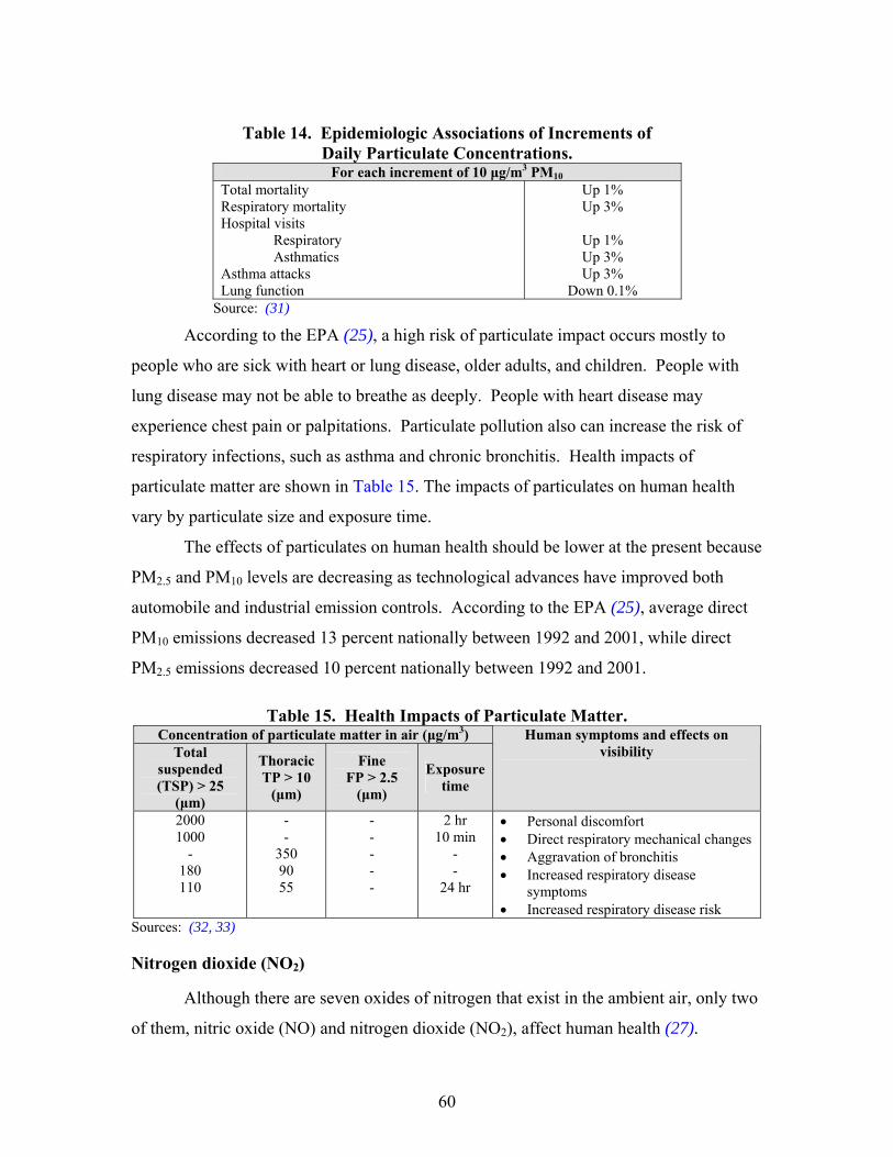
60
Table 14. Epidemiologic Associations of Increments of Daily Particulate Concentrations.
For each increment of 10 μg/m3 PM10 Total mortality Respiratory mortality Hospital visits
Respiratory Asthmatics
Asthma attacks Lung function
Up 1% Up 3%
Up 1% Up 3% Up 3%
Down 0.1% Source: (31)
According to the EPA (25), a high risk of particulate impact occurs mostly to
people who are sick with heart or lung disease, older adults, and children. People with
lung disease may not be able to breathe as deeply. People with heart disease may
experience chest pain or palpitations. Particulate pollution also can increase the risk of
respiratory infections, such as asthma and chronic bronchitis. Health impacts of
particulate matter are shown in Table 15. The impacts of particulates on human health
vary by particulate size and exposure time.
The effects of particulates on human health should be lower at the present because
PM2.5 and PM10 levels are decreasing as technological advances have improved both
automobile and industrial emission controls. According to the EPA (25), average direct
PM10 emissions decreased 13 percent nationally between 1992 and 2001, while direct
PM2.5 emissions decreased 10 percent nationally between 1992 and 2001.
Table 15. Health Impacts of Particulate Matter. Concentration of particulate matter in air (μg/m3)
Total suspended (TSP) > 25
(μm)
Thoracic TP > 10
(μm)
Fine FP > 2.5
(μm)
Exposure time
Human symptoms and effects on visibility
2000 1000
- 180 110
- -
350 90 55
- - - - -
2 hr 10 min
- -
24 hr
• Personal discomfort • Direct respiratory mechanical changes • Aggravation of bronchitis • Increased respiratory disease
symptoms • Increased respiratory disease risk
Sources: (32, 33)
Nitrogen dioxide (NO2)
Although there are seven oxides of nitrogen that exist in the ambient air, only two
of them, nitric oxide (NO) and nitrogen dioxide (NO2), affect human health (27).
RESUBMITTAL
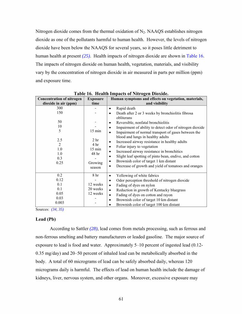
61
Nitrogen dioxide comes from the thermal oxidation of N2. NAAQS establishes nitrogen
dioxide as one of the pollutants harmful to human health. However, the levels of nitrogen
dioxide have been below the NAAQS for several years, so it poses little detriment to
human health at present (25). Health impacts of nitrogen dioxide are shown in Table 16.
The impacts of nitrogen dioxide on human health, vegetation, materials, and visibility
vary by the concentration of nitrogen dioxide in air measured in parts per million (ppm)
and exposure time.
Table 16. Health Impacts of Nitrogen Dioxide. Concentration of nitrogen
dioxide in air (ppm) Exposure
time Human symptoms and effects on vegetation, materials,
and visibility 300 150
50 10 5
2.5 2
1.0 1.0 0.3
0.25
- - - -
15 min
2 hr 4 hr
15 min 48 hr
- Growing season
• Rapid death • Death after 2 or 3 weeks by bronchiolitis fibrosa
obliterans • Reversible, nonfatal bronchiolitis • Impairment of ability to detect odor of nitrogen dioxide • Impairment of normal transport of gases between the
blood and lungs in healthy adults • Increased airway resistance in healthy adults • Foliar injury to vegetation • Increased airway resistance in bronchitics • Slight leaf spotting of pinto bean, endive, and cotton • Brownish color of target 1 km distant • Decrease of growth and yield of tomatoes and oranges
0.2 0.12 0.1 0.1
0.05 0.03 0.003
8 hr -
12 weeks 20 weeks 12 weeks
- -
• Yellowing of white fabrics • Odor perception threshold of nitrogen dioxide • Fading of dyes on nylon • Reduction in growth of Kentucky bluegrass • Fading of dyes on cotton and rayon • Brownish color of target 10 km distant • Brownish color of target 100 km distant
Sources: (34, 35)
Lead (Pb)
According to Sattler (28), lead comes from metals processing, such as ferrous and
non-ferrous smelting and battery manufacturers or leaded gasoline. The major source of
exposure to lead is food and water. Approximately 5–10 percent of ingested lead (0.12-
0.35 mg/day) and 20–50 percent of inhaled lead can be metabolically absorbed in the
body. A total of 60 micrograms of lead can be safely absorbed daily, whereas 120
micrograms daily is harmful. The effects of lead on human health include the damage of
kidneys, liver, nervous system, and other organs. Moreover, excessive exposure may
RESUBMITTAL
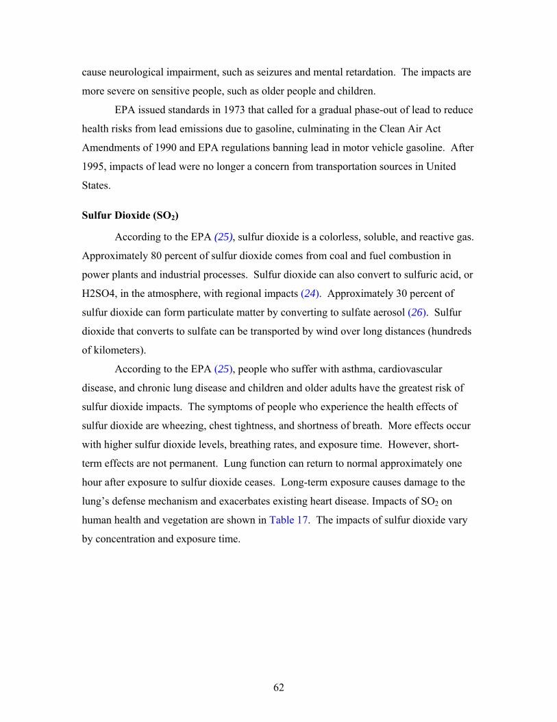
62
cause neurological impairment, such as seizures and mental retardation. The impacts are
more severe on sensitive people, such as older people and children.
EPA issued standards in 1973 that called for a gradual phase-out of lead to reduce
health risks from lead emissions due to gasoline, culminating in the Clean Air Act
Amendments of 1990 and EPA regulations banning lead in motor vehicle gasoline. After
1995, impacts of lead were no longer a concern from transportation sources in United
States.
Sulfur Dioxide (SO2)
According to the EPA (25), sulfur dioxide is a colorless, soluble, and reactive gas.
Approximately 80 percent of sulfur dioxide comes from coal and fuel combustion in
power plants and industrial processes. Sulfur dioxide can also convert to sulfuric acid, or
H2SO4, in the atmosphere, with regional impacts (24). Approximately 30 percent of
sulfur dioxide can form particulate matter by converting to sulfate aerosol (26). Sulfur
dioxide that converts to sulfate can be transported by wind over long distances (hundreds
of kilometers).
According to the EPA (25), people who suffer with asthma, cardiovascular
disease, and chronic lung disease and children and older adults have the greatest risk of
sulfur dioxide impacts. The symptoms of people who experience the health effects of
sulfur dioxide are wheezing, chest tightness, and shortness of breath. More effects occur
with higher sulfur dioxide levels, breathing rates, and exposure time. However, short-
term effects are not permanent. Lung function can return to normal approximately one
hour after exposure to sulfur dioxide ceases. Long-term exposure causes damage to the
lung’s defense mechanism and exacerbates existing heart disease. Impacts of SO2 on
human health and vegetation are shown in Table 17. The impacts of sulfur dioxide vary
by concentration and exposure time.
RESUBMITTAL
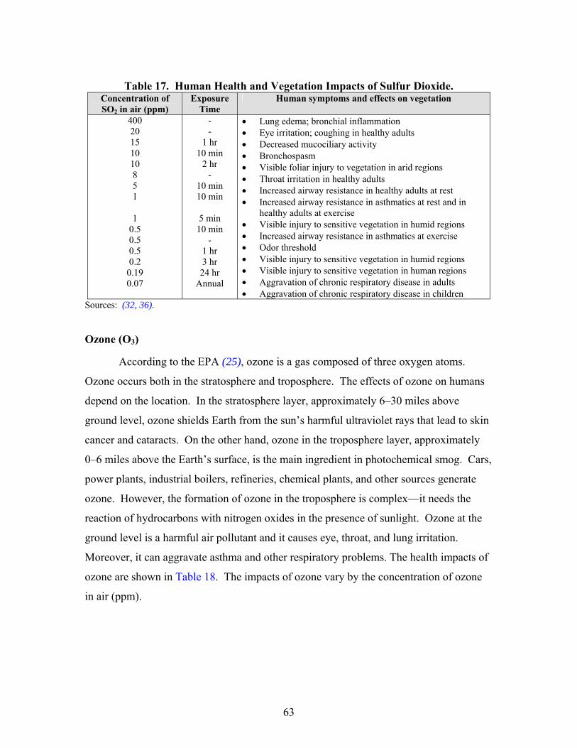
63
Table 17. Human Health and Vegetation Impacts of Sulfur Dioxide. Concentration of SO2 in air (ppm)
Exposure Time
Human symptoms and effects on vegetation
400 20 15 10 10 8 5 1
1 0.5 0.5 0.5 0.2
0.19 0.07
- -
1 hr 10 min
2 hr -
10 min 10 min
5 min
10 min -
1 hr 3 hr 24 hr
Annual
• Lung edema; bronchial inflammation • Eye irritation; coughing in healthy adults • Decreased mucociliary activity • Bronchospasm • Visible foliar injury to vegetation in arid regions • Throat irritation in healthy adults • Increased airway resistance in healthy adults at rest • Increased airway resistance in asthmatics at rest and in
healthy adults at exercise • Visible injury to sensitive vegetation in humid regions • Increased airway resistance in asthmatics at exercise • Odor threshold • Visible injury to sensitive vegetation in humid regions • Visible injury to sensitive vegetation in human regions • Aggravation of chronic respiratory disease in adults • Aggravation of chronic respiratory disease in children
Sources: (32, 36).
Ozone (O3)
According to the EPA (25), ozone is a gas composed of three oxygen atoms.
Ozone occurs both in the stratosphere and troposphere. The effects of ozone on humans
depend on the location. In the stratosphere layer, approximately 6–30 miles above
ground level, ozone shields Earth from the sun’s harmful ultraviolet rays that lead to skin
cancer and cataracts. On the other hand, ozone in the troposphere layer, approximately
0–6 miles above the Earth’s surface, is the main ingredient in photochemical smog. Cars,
power plants, industrial boilers, refineries, chemical plants, and other sources generate
ozone. However, the formation of ozone in the troposphere is complex—it needs the
reaction of hydrocarbons with nitrogen oxides in the presence of sunlight. Ozone at the
ground level is a harmful air pollutant and it causes eye, throat, and lung irritation.
Moreover, it can aggravate asthma and other respiratory problems. The health impacts of
ozone are shown in Table 18. The impacts of ozone vary by the concentration of ozone
in air (ppm).
RESUBMITTAL
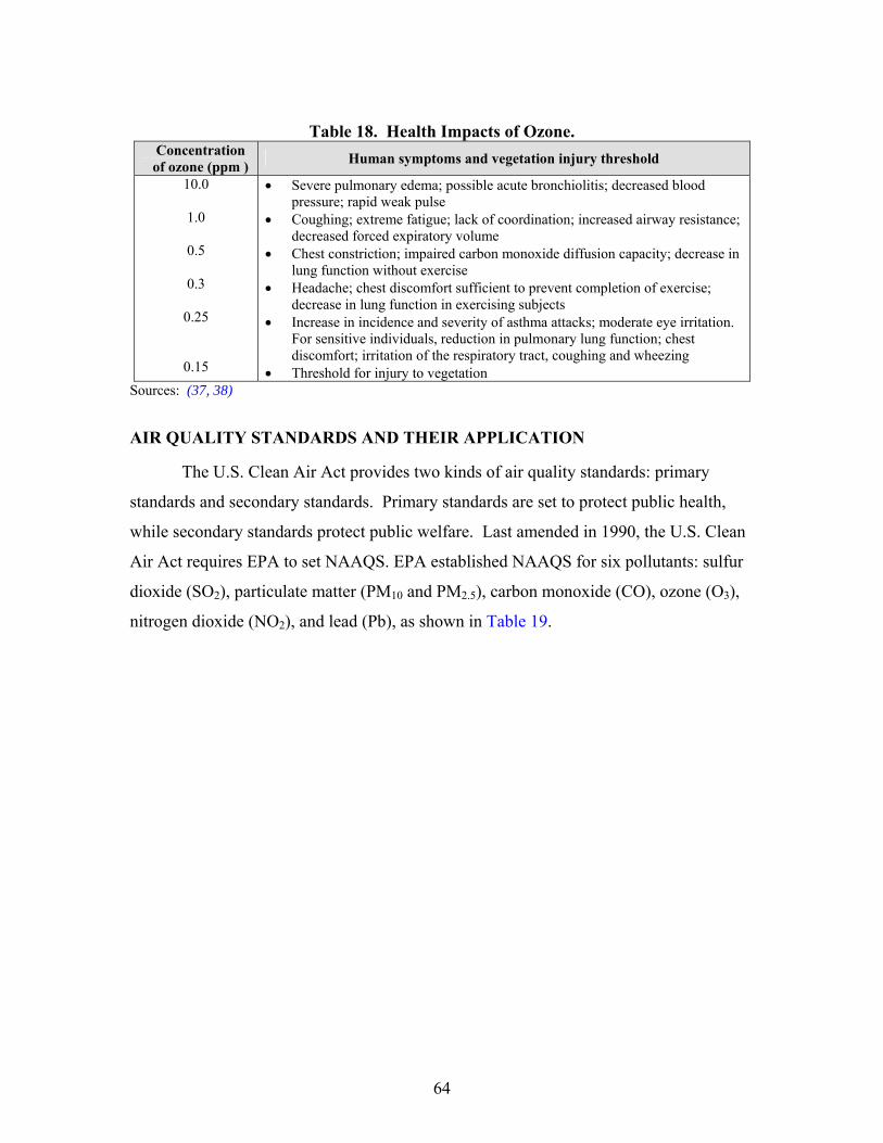
64
Table 18. Health Impacts of Ozone. Concentration of ozone (ppm ) Human symptoms and vegetation injury threshold
10.0
1.0
0.5
0.3
0.25
0.15
• Severe pulmonary edema; possible acute bronchiolitis; decreased blood pressure; rapid weak pulse
• Coughing; extreme fatigue; lack of coordination; increased airway resistance; decreased forced expiratory volume
• Chest constriction; impaired carbon monoxide diffusion capacity; decrease in lung function without exercise
• Headache; chest discomfort sufficient to prevent completion of exercise; decrease in lung function in exercising subjects
• Increase in incidence and severity of asthma attacks; moderate eye irritation. For sensitive individuals, reduction in pulmonary lung function; chest discomfort; irritation of the respiratory tract, coughing and wheezing
• Threshold for injury to vegetation Sources: (37, 38)
AIR QUALITY STANDARDS AND THEIR APPLICATION
The U.S. Clean Air Act provides two kinds of air quality standards: primary
standards and secondary standards. Primary standards are set to protect public health,
while secondary standards protect public welfare. Last amended in 1990, the U.S. Clean
Air Act requires EPA to set NAAQS. EPA established NAAQS for six pollutants: sulfur
dioxide (SO2), particulate matter (PM10 and PM2.5), carbon monoxide (CO), ozone (O3),
nitrogen dioxide (NO2), and lead (Pb), as shown in Table 19.
RESUBMITTAL
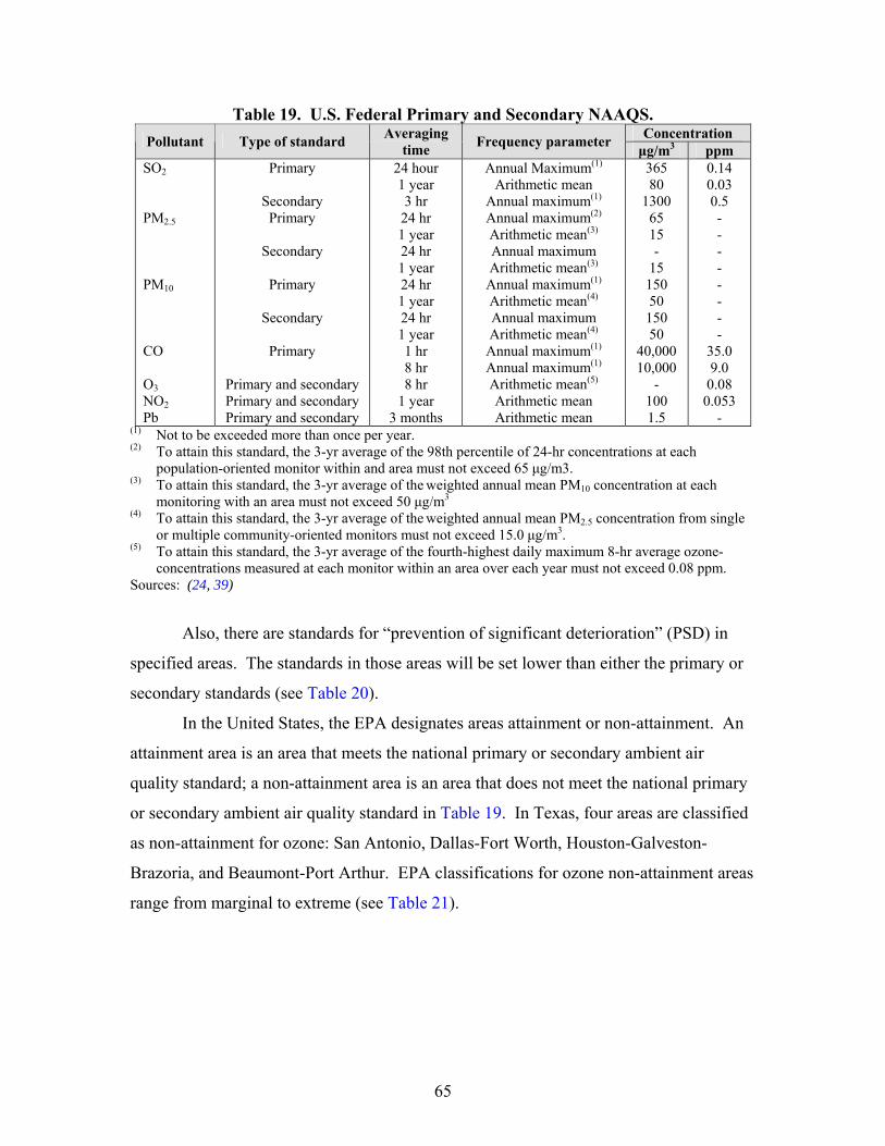
65
Table 19. U.S. Federal Primary and Secondary NAAQS. Concentration Pollutant Type of standard Averaging
time Frequency parameter μg/m3 ppm SO2 PM2.5
PM10
CO O3 NO2 Pb
Primary
Secondary Primary
Secondary
Primary
Secondary
Primary
Primary and secondary Primary and secondary Primary and secondary
24 hour 1 year 3 hr
24 hr 1 year 24 hr 1 year 24 hr 1 year 24 hr 1 year 1 hr 8 hr 8 hr
1 year 3 months
Annual Maximum(1)
Arithmetic mean Annual maximum(1)
Annual maximum(2)
Arithmetic mean(3) Annual maximum Arithmetic mean(3) Annual maximum(1)
Arithmetic mean(4) Annual maximum Arithmetic mean(4) Annual maximum(1)
Annual maximum(1)
Arithmetic mean(5)
Arithmetic mean Arithmetic mean
365 80
1300 65 15 -
15 150 50 150 50
40,000 10,000
- 100 1.5
0.14 0.03 0.5 - - - - - - - -
35.0 9.0
0.08 0.053
- (1) Not to be exceeded more than once per year. (2) To attain this standard, the 3-yr average of the 98th percentile of 24-hr concentrations at each
population-oriented monitor within and area must not exceed 65 μg/m3. (3) To attain this standard, the 3-yr average of the weighted annual mean PM10 concentration at each
monitoring with an area must not exceed 50 μg/m3 (4) To attain this standard, the 3-yr average of the weighted annual mean PM2.5 concentration from single
or multiple community-oriented monitors must not exceed 15.0 μg/m3. (5) To attain this standard, the 3-yr average of the fourth-highest daily maximum 8-hr average ozone-
concentrations measured at each monitor within an area over each year must not exceed 0.08 ppm. Sources: (24, 39)
Also, there are standards for “prevention of significant deterioration” (PSD) in
specified areas. The standards in those areas will be set lower than either the primary or
secondary standards (see Table 20).
In the United States, the EPA designates areas attainment or non-attainment. An
attainment area is an area that meets the national primary or secondary ambient air
quality standard; a non-attainment area is an area that does not meet the national primary
or secondary ambient air quality standard in Table 19. In Texas, four areas are classified
as non-attainment for ozone: San Antonio, Dallas-Fort Worth, Houston-Galveston-
Brazoria, and Beaumont-Port Arthur. EPA classifications for ozone non-attainment areas
range from marginal to extreme (see Table 21).
RESUBMITTAL
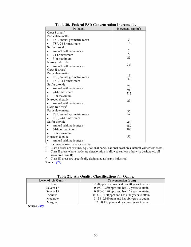
66
Table 20. Federal PSD Concentration Increments. Pollutant Incrementa (μg/m3)
Class I areasb Particulate matter • TSP, annual geometric mean • TSP, 24-hr maximum Sulfur dioxide • Annual arithmetic mean • 24-hr maximum • 3-hr maximum Nitrogen dioxide • Annual arithmetic mean Class II areasc Particulate matter • TSP, annual geometric mean • TSP, 24-hr maximum Sulfur dioxide • Annual arithmetic mean • 24-hr maximum • 3-hr maximum Nitrogen dioxide • Annual arithmetic mean Class III areasd Particulate matter • TSP, annual geometric mean • TSP, 24-hr maximum Sulfur dioxide • Annual arithmetic mean • 24-hour maximum • 3-hr maximum Nitrogen dioxide • Annual arithmetic mean
5 10
2 5
25
2.5
19 37
20 91 512
25
37 75
40 182 700
50
(a) Increments over base air quality (b) Class I areas are pristine, e.g., national parks, national seashores, natural wilderness areas. (c) Class II areas where moderate deterioration is allowed (unless otherwise designated, all
areas are Class II). (d) Class III areas are specifically designated as heavy industrial. Source: (24)
Table 21. Air Quality Classifications for Ozone. Level of Air Quality Concentration (ppm)
Extreme Severe 17 Severe 15 Serious
Moderate Marginal
0.280 ppm or above and has 20 years to attain. 0.190–0.280 ppm and has 17 years to attain. 0.180–0.190 ppm and has 15 years to attain.
0.160–0.180 ppm and has nine years to attain. 0.138–0.160 ppm and has six years to attain.
0.121–0.138 ppm and has three years to attain. Source: (40)
RESUBMITTAL
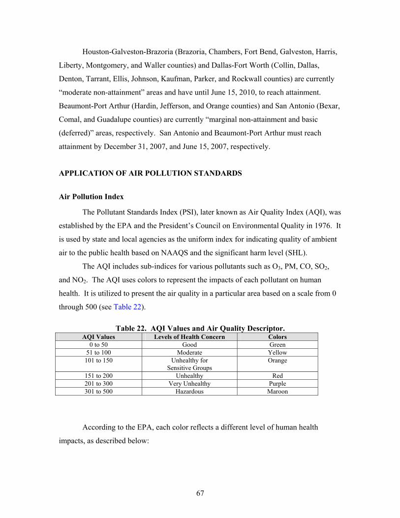
67
Houston-Galveston-Brazoria (Brazoria, Chambers, Fort Bend, Galveston, Harris,
Liberty, Montgomery, and Waller counties) and Dallas-Fort Worth (Collin, Dallas,
Denton, Tarrant, Ellis, Johnson, Kaufman, Parker, and Rockwall counties) are currently
“moderate non-attainment” areas and have until June 15, 2010, to reach attainment.
Beaumont-Port Arthur (Hardin, Jefferson, and Orange counties) and San Antonio (Bexar,
Comal, and Guadalupe counties) are currently “marginal non-attainment and basic
(deferred)” areas, respectively. San Antonio and Beaumont-Port Arthur must reach
attainment by December 31, 2007, and June 15, 2007, respectively.
APPLICATION OF AIR POLLUTION STANDARDS
Air Pollution Index
The Pollutant Standards Index (PSI), later known as Air Quality Index (AQI), was
established by the EPA and the President’s Council on Environmental Quality in 1976. It
is used by state and local agencies as the uniform index for indicating quality of ambient
air to the public health based on NAAQS and the significant harm level (SHL).
The AQI includes sub-indices for various pollutants such as O3, PM, CO, SO2,
and NO2. The AQI uses colors to represent the impacts of each pollutant on human
health. It is utilized to present the air quality in a particular area based on a scale from 0
through 500 (see Table 22).
Table 22. AQI Values and Air Quality Descriptor. AQI Values Levels of Health Concern Colors
0 to 50 Good Green 51 to 100 Moderate Yellow 101 to 150 Unhealthy for
Sensitive Groups Orange
151 to 200 Unhealthy Red 201 to 300 Very Unhealthy Purple 301 to 500 Hazardous Maroon
According to the EPA, each color reflects a different level of human health
impacts, as described below:
RESUBMITTAL
68
• “Good” – An AQI value between 0 and 50 represents satisfactory air
quality, and air pollution poses little or no risk.
• “Moderate” – An AQI value between 51 and 100 represents acceptable
conditions; however, some pollutants may present a moderate health
concern for a very small number of people. For example, people who are
unusually sensitive to ozone may experience respiratory symptoms.
• “Unhealthy for Sensitive Groups” – AQI values between 101 and 150 may
affect some sensitive groups of people, such as people with lung or heart
disease, children, and elderly people.
• “Unhealthy” – Everyone may begin to experience health effects when AQI
values are between 151 and 200. Members of sensitive groups may
experience more serious health effects.
• “Very Unhealthy” – AQI values between 201 and 300 trigger a health alert,
meaning everyone may experience more serious health effects.
• “Hazardous” – AQI values over 300 trigger health warnings of emergency
conditions. The entire population is more likely to be affected.
When the pollutant has an index value above 100, ozone will affect more sensitive
people including children and people with asthma. PM2.5 will affect people with
respiratory or heart disease, the elderly, and children. PM10 will affect people with
respiratory disease. CO will affect people with heart disease. SO2 will affect people with
asthma. Index values between 200 and 400 are defined as alert, warning, and emergency
levels. An index value of 500 indicates severe related impacts including death.
Recently, the EPA has been developing new and innovative programs in order to
provide more information for the public through the Ozone Mapping Project and
community action programs. The program can provide real-time AQI reporting to the
public. Ozone mapping is used in 31 states including 1500 monitors across the eastern
and central United States and California.
AQI Procedure
a) Identify the highest concentration pollutants.
RESUBMITTAL
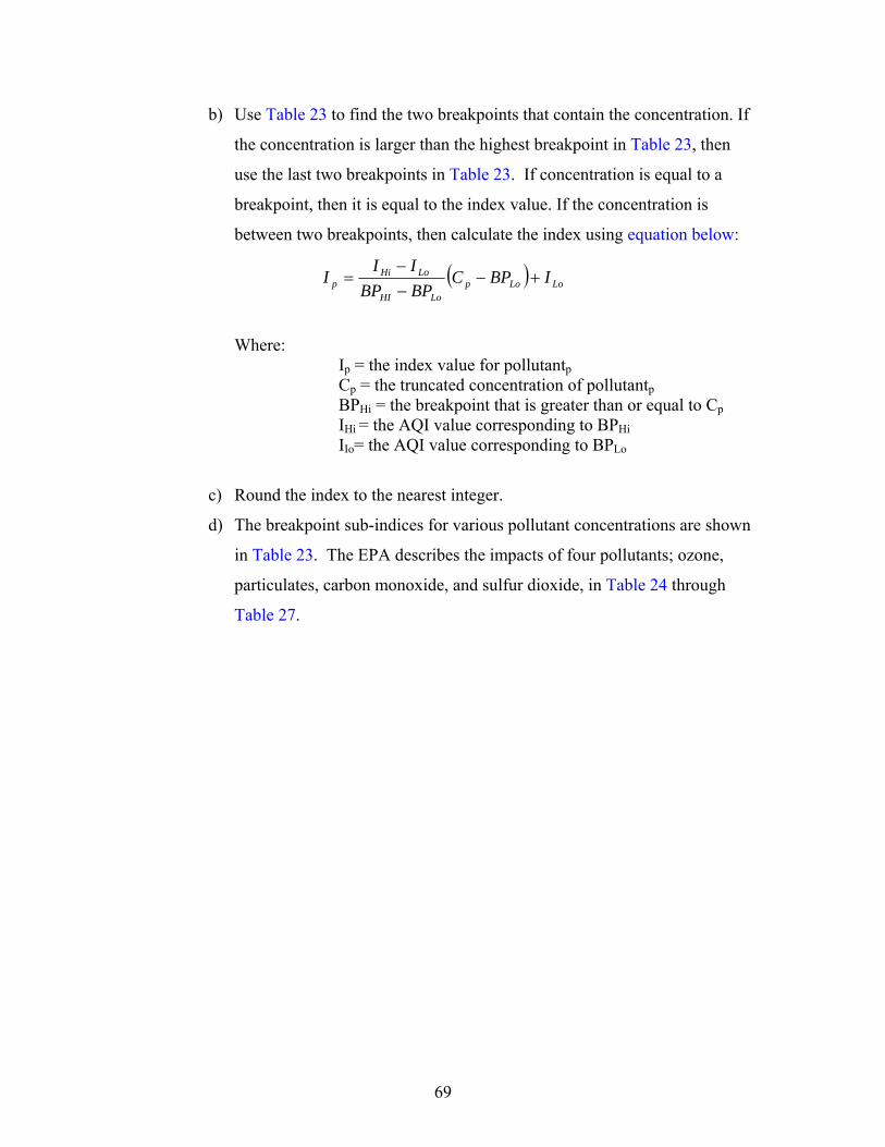
69
b) Use Table 23 to find the two breakpoints that contain the concentration. If
the concentration is larger than the highest breakpoint in Table 23, then
use the last two breakpoints in Table 23. If concentration is equal to a
breakpoint, then it is equal to the index value. If the concentration is
between two breakpoints, then calculate the index using equation below:
( ) LoLopLoHI
LoHip IBPC
BPBPII
I +−−−
=
Where:
Ip = the index value for pollutantp Cp = the truncated concentration of pollutantp BPHi = the breakpoint that is greater than or equal to Cp IHi = the AQI value corresponding to BPHi IIo= the AQI value corresponding to BPLo
c) Round the index to the nearest integer.
d) The breakpoint sub-indices for various pollutant concentrations are shown
in Table 23. The EPA describes the impacts of four pollutants; ozone,
particulates, carbon monoxide, and sulfur dioxide, in Table 24 through
Table 27.
RESUBMITTAL
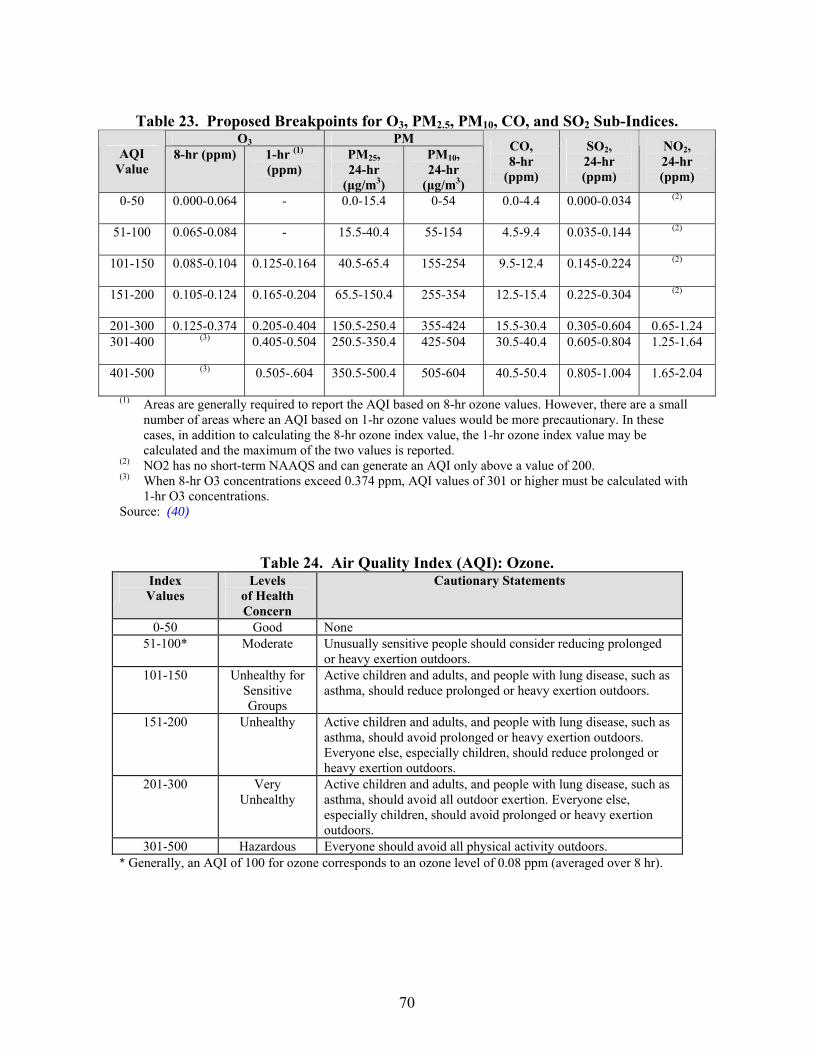
70
Table 23. Proposed Breakpoints for O3, PM2.5, PM10, CO, and SO2 Sub-Indices. O3 PM
AQI Value
8-hr (ppm) 1-hr (1) (ppm)
PM25, 24-hr
(μg/m3)
PM10, 24-hr
(μg/m3)
CO, 8-hr
(ppm)
SO2, 24-hr (ppm)
NO2, 24-hr (ppm)
0-50
0.000-0.064 -
0.0-15.4 0-54 0.0-4.4 0.000-0.034 (2)
51-100
0.065-0.084 -
15.5-40.4 55-154 4.5-9.4 0.035-0.144 (2)
101-150 0.085-0.104 0.125-0.164 40.5-65.4 155-254 9.5-12.4 0.145-0.224 (2)
151-200 0.105-0.124 0.165-0.204 65.5-150.4 255-354 12.5-15.4 0.225-0.304 (2)
201-300 0.125-0.374 0.205-0.404 150.5-250.4 355-424 15.5-30.4 0.305-0.604 0.65-1.24
301-400 (3)
0.405-0.504 250.5-350.4 425-504 30.5-40.4 0.605-0.804 1.25-1.64
401-500 (3)
0.505-.604 350.5-500.4 505-604 40.5-50.4 0.805-1.004 1.65-2.04
(1) Areas are generally required to report the AQI based on 8-hr ozone values. However, there are a small number of areas where an AQI based on 1-hr ozone values would be more precautionary. In these cases, in addition to calculating the 8-hr ozone index value, the 1-hr ozone index value may be calculated and the maximum of the two values is reported.
(2) NO2 has no short-term NAAQS and can generate an AQI only above a value of 200. (3) When 8-hr O3 concentrations exceed 0.374 ppm, AQI values of 301 or higher must be calculated with
1-hr O3 concentrations. Source: (40)
Table 24. Air Quality Index (AQI): Ozone. Index Values
Levels of Health Concern
Cautionary Statements
0-50 Good None 51-100* Moderate Unusually sensitive people should consider reducing prolonged
or heavy exertion outdoors. 101-150 Unhealthy for
Sensitive Groups
Active children and adults, and people with lung disease, such as asthma, should reduce prolonged or heavy exertion outdoors.
151-200 Unhealthy Active children and adults, and people with lung disease, such as asthma, should avoid prolonged or heavy exertion outdoors. Everyone else, especially children, should reduce prolonged or heavy exertion outdoors.
201-300 Very Unhealthy
Active children and adults, and people with lung disease, such as asthma, should avoid all outdoor exertion. Everyone else, especially children, should avoid prolonged or heavy exertion outdoors.
301-500 Hazardous Everyone should avoid all physical activity outdoors. * Generally, an AQI of 100 for ozone corresponds to an ozone level of 0.08 ppm (averaged over 8 hr).
RESUBMITTAL
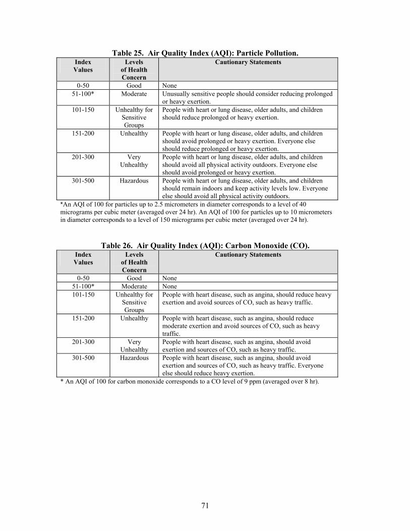
71
Table 25. Air Quality Index (AQI): Particle Pollution. Index Values
Levels of Health Concern
Cautionary Statements
0-50 Good None 51-100* Moderate Unusually sensitive people should consider reducing prolonged
or heavy exertion. 101-150 Unhealthy for
Sensitive Groups
People with heart or lung disease, older adults, and children should reduce prolonged or heavy exertion.
151-200 Unhealthy People with heart or lung disease, older adults, and children should avoid prolonged or heavy exertion. Everyone else should reduce prolonged or heavy exertion.
201-300 Very Unhealthy
People with heart or lung disease, older adults, and children should avoid all physical activity outdoors. Everyone else should avoid prolonged or heavy exertion.
301-500 Hazardous People with heart or lung disease, older adults, and children should remain indoors and keep activity levels low. Everyone else should avoid all physical activity outdoors.
*An AQI of 100 for particles up to 2.5 micrometers in diameter corresponds to a level of 40 micrograms per cubic meter (averaged over 24 hr). An AQI of 100 for particles up to 10 micrometers in diameter corresponds to a level of 150 micrograms per cubic meter (averaged over 24 hr).
Table 26. Air Quality Index (AQI): Carbon Monoxide (CO). Index Values
Levels of Health Concern
Cautionary Statements
0-50 Good None 51-100* Moderate None 101-150 Unhealthy for
Sensitive Groups
People with heart disease, such as angina, should reduce heavy exertion and avoid sources of CO, such as heavy traffic.
151-200 Unhealthy People with heart disease, such as angina, should reduce moderate exertion and avoid sources of CO, such as heavy traffic.
201-300 Very Unhealthy
People with heart disease, such as angina, should avoid exertion and sources of CO, such as heavy traffic.
301-500 Hazardous People with heart disease, such as angina, should avoid exertion and sources of CO, such as heavy traffic. Everyone else should reduce heavy exertion.
* An AQI of 100 for carbon monoxide corresponds to a CO level of 9 ppm (averaged over 8 hr).
RESUBMITTAL
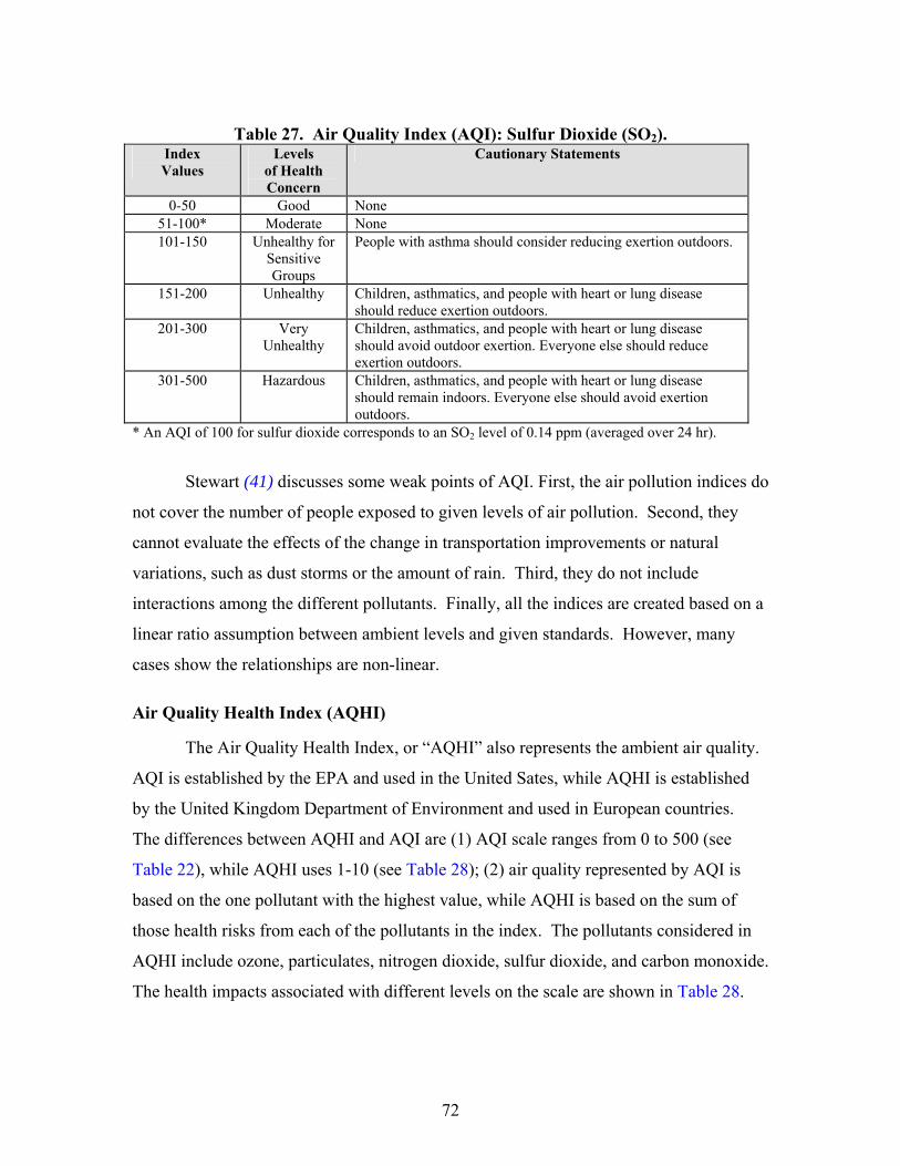
72
Table 27. Air Quality Index (AQI): Sulfur Dioxide (SO2). Index Values
Levels of Health Concern
Cautionary Statements
0-50 Good None 51-100* Moderate None 101-150 Unhealthy for
Sensitive Groups
People with asthma should consider reducing exertion outdoors.
151-200 Unhealthy Children, asthmatics, and people with heart or lung disease should reduce exertion outdoors.
201-300 Very Unhealthy
Children, asthmatics, and people with heart or lung disease should avoid outdoor exertion. Everyone else should reduce exertion outdoors.
301-500 Hazardous Children, asthmatics, and people with heart or lung disease should remain indoors. Everyone else should avoid exertion outdoors.
* An AQI of 100 for sulfur dioxide corresponds to an SO2 level of 0.14 ppm (averaged over 24 hr).
Stewart (41) discusses some weak points of AQI. First, the air pollution indices do
not cover the number of people exposed to given levels of air pollution. Second, they
cannot evaluate the effects of the change in transportation improvements or natural
variations, such as dust storms or the amount of rain. Third, they do not include
interactions among the different pollutants. Finally, all the indices are created based on a
linear ratio assumption between ambient levels and given standards. However, many
cases show the relationships are non-linear.
Air Quality Health Index (AQHI)
The Air Quality Health Index, or “AQHI” also represents the ambient air quality.
AQI is established by the EPA and used in the United Sates, while AQHI is established
by the United Kingdom Department of Environment and used in European countries.
The differences between AQHI and AQI are (1) AQI scale ranges from 0 to 500 (see
Table 22), while AQHI uses 1-10 (see Table 28); (2) air quality represented by AQI is
based on the one pollutant with the highest value, while AQHI is based on the sum of
those health risks from each of the pollutants in the index. The pollutants considered in
AQHI include ozone, particulates, nitrogen dioxide, sulfur dioxide, and carbon monoxide.
The health impacts associated with different levels on the scale are shown in Table 28.
RESUBMITTAL
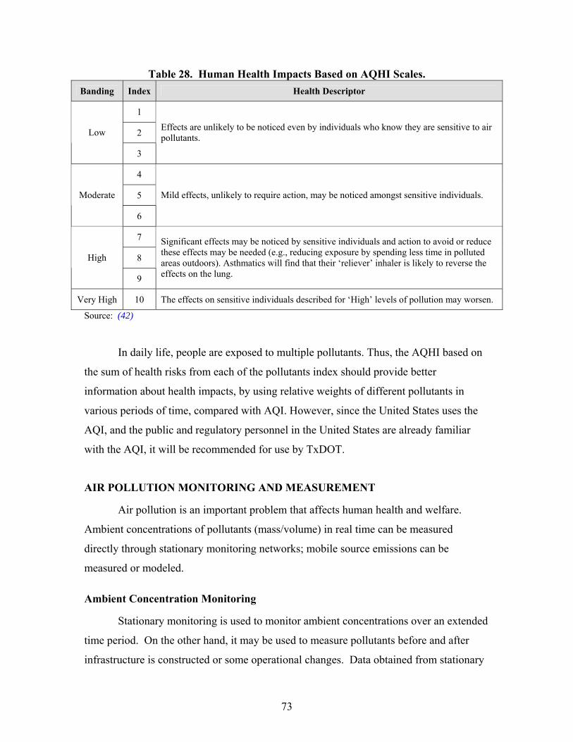
73
Table 28. Human Health Impacts Based on AQHI Scales. Banding Index Health Descriptor
1
2 Low
3
Effects are unlikely to be noticed even by individuals who know they are sensitive to air pollutants.
4
5 Moderate
6
Mild effects, unlikely to require action, may be noticed amongst sensitive individuals.
7
8 High
9
Significant effects may be noticed by sensitive individuals and action to avoid or reduce these effects may be needed (e.g., reducing exposure by spending less time in polluted areas outdoors). Asthmatics will find that their ‘reliever’ inhaler is likely to reverse the effects on the lung.
Very High 10 The effects on sensitive individuals described for ‘High’ levels of pollution may worsen.
Source: (42)
In daily life, people are exposed to multiple pollutants. Thus, the AQHI based on
the sum of health risks from each of the pollutants index should provide better
information about health impacts, by using relative weights of different pollutants in
various periods of time, compared with AQI. However, since the United States uses the
AQI, and the public and regulatory personnel in the United States are already familiar
with the AQI, it will be recommended for use by TxDOT.
AIR POLLUTION MONITORING AND MEASUREMENT
Air pollution is an important problem that affects human health and welfare.
Ambient concentrations of pollutants (mass/volume) in real time can be measured
directly through stationary monitoring networks; mobile source emissions can be
measured or modeled.
Ambient Concentration Monitoring
Stationary monitoring is used to monitor ambient concentrations over an extended
time period. On the other hand, it may be used to measure pollutants before and after
infrastructure is constructed or some operational changes. Data obtained from stationary
RESUBMITTAL
74
monitoring include the concentration of various air pollutants and weather conditions,
such as temperature, wind speed, and wind direction.
According to the EPA, monitoring stations in the United States are utilized for
many purposes. The network of monitoring stations is used to assess the air quality at
local, regional, and national levels; assess the heath impacts, effectiveness of control
programs, and source impacts; help form the basis for new control programs; and provide
information to the public. The EPA’s ambient air quality monitoring program establishes
four categories of monitoring stations:
• Photochemical Assessment Monitoring Stations (PAMS) – measure ozone
precursors (volatile organic compounds [VOCs] and nitrogen oxides [NOx],
which react to form ozone);
• State and Local Air Monitoring Stations (SLAMS) – obtain air pollution
information in strategic locations across the nation;
• National Air Monitoring Stations (NAMS) – a part of the SLAMS network
added in order to obtain more detailed information; and
• Special Purpose Monitoring Stations (SPMS) – measure air pollution for
short-term monitoring.
The pollutants being measured through monitoring sites are carbon monoxide,
ozone, nitrogen oxides, PM10, lead, sulfur dioxide, and, in some cases VOCs. Table 29
describes national monitoring networks, including sampling frequency. Several networks
in addition to PAMS, SLAMS, and NAMS are also described.
RESUBMITTAL
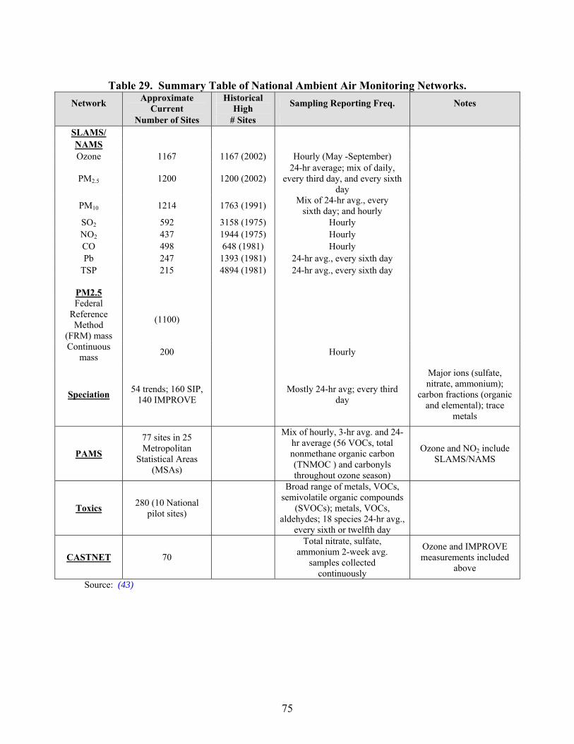
75
Table 29. Summary Table of National Ambient Air Monitoring Networks. Network Approximate
Current Historical
High Sampling Reporting Freq. Notes
Number of Sites # Sites SLAMS/ NAMS Ozone 1167 1167 (2002) Hourly (May -September)
PM2.5 1200 1200 (2002) 24-hr average; mix of daily,
every third day, and every sixth day
PM10 1214 1763 (1991) Mix of 24-hr avg., every sixth day; and hourly
SO2 592 3158 (1975) Hourly NO2 437 1944 (1975) Hourly CO 498 648 (1981) Hourly Pb 247 1393 (1981) 24-hr avg., every sixth day
TSP 215 4894 (1981) 24-hr avg., every sixth day
PM2.5
Federal Reference Method
(FRM) mass
(1100)
Continuous mass 200 Hourly
Speciation 54 trends; 160 SIP, 140 IMPROVE Mostly 24-hr avg; every third
day
Major ions (sulfate, nitrate, ammonium);
carbon fractions (organic and elemental); trace
metals
PAMS
77 sites in 25 Metropolitan
Statistical Areas (MSAs)
Mix of hourly, 3-hr avg. and 24-hr average (56 VOCs, total nonmethane organic carbon (TNMOC ) and carbonyls throughout ozone season)
Ozone and NO2 include SLAMS/NAMS
Toxics 280 (10 National pilot sites)
Broad range of metals, VOCs, semivolatile organic compounds
(SVOCs); metals, VOCs, aldehydes; 18 species 24-hr avg.,
every sixth or twelfth day
CASTNET 70
Total nitrate, sulfate, ammonium 2-week avg.
samples collected continuously
Ozone and IMPROVE measurements included
above
Source: (43)
RESUBMITTAL
76
State environmental agencies, local Air Pollution Control Districts (APCDs),
cities, private contractors, and the National Parks Service (NPS) are responsible for
operating NAMS, PAMS, SLAMS, and SPMS. Data from the monitoring sites may
include (based on purposes of data collection):
• The concentration of ozone, CO, NO2, SO2, PM2.5, PM10, VOCs, lead; light
scatter monitored with nephelometer; nonmethane hydrocarbons (total)
collected in continuous monitors, nonmethane hydrocarbons (speciated)
collected in canisters (3-hour or 24-hour samples); and total hydrocarbons
monitored by continuous analyzer
• Meteorological data
o dew point temperature
o barometric pressure
o relative humidity
o total solar radiation
o ambient air temperature
o ultraviolet radiation
o vertical wind speed
o wind direction
o wind speed
Sampling or analysis methods may include:
• atomic absorption spectroscopy – graphite oven from high-volume sampler;
• chemiluminescence;
• colormetric;
• conductimetric;
• emission spectrometry ICAP (inductively coupled argon plasma);
• fluorescence;
• flame photometric;
• gas chromatography;
• inductively coupled plasma-mass spectrometer;
• nondispersive infrared;
RESUBMITTAL
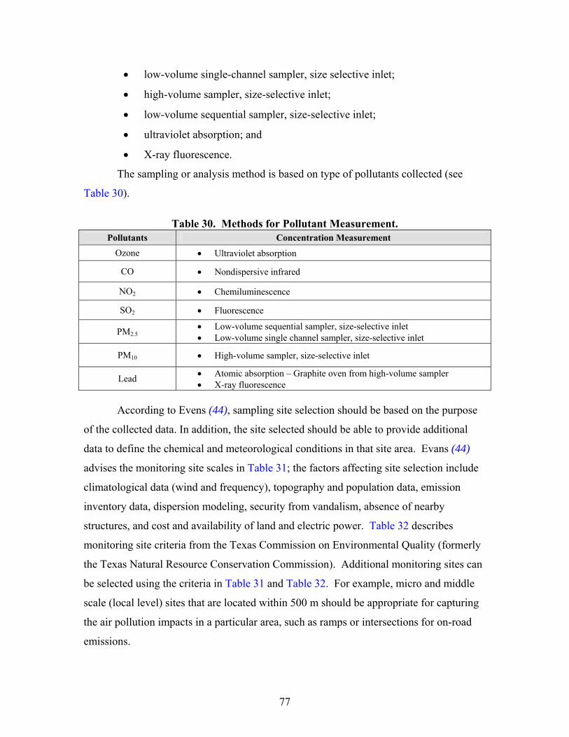
77
• low-volume single-channel sampler, size selective inlet;
• high-volume sampler, size-selective inlet;
• low-volume sequential sampler, size-selective inlet;
• ultraviolet absorption; and
• X-ray fluorescence.
The sampling or analysis method is based on type of pollutants collected (see
Table 30).
Table 30. Methods for Pollutant Measurement. Pollutants Concentration Measurement
Ozone • Ultraviolet absorption
CO • Nondispersive infrared
NO2 • Chemiluminescence
SO2 • Fluorescence
PM2.5 • Low-volume sequential sampler, size-selective inlet • Low-volume single channel sampler, size-selective inlet
PM10 • High-volume sampler, size-selective inlet
Lead • Atomic absorption – Graphite oven from high-volume sampler • X-ray fluorescence
According to Evens (44), sampling site selection should be based on the purpose
of the collected data. In addition, the site selected should be able to provide additional
data to define the chemical and meteorological conditions in that site area. Evans (44)
advises the monitoring site scales in Table 31; the factors affecting site selection include
climatological data (wind and frequency), topography and population data, emission
inventory data, dispersion modeling, security from vandalism, absence of nearby
structures, and cost and availability of land and electric power. Table 32 describes
monitoring site criteria from the Texas Commission on Environmental Quality (formerly
the Texas Natural Resource Conservation Commission). Additional monitoring sites can
be selected using the criteria in Table 31 and Table 32. For example, micro and middle
scale (local level) sites that are located within 500 m should be appropriate for capturing
the air pollution impacts in a particular area, such as ramps or intersections for on-road
emissions.
RESUBMITTAL
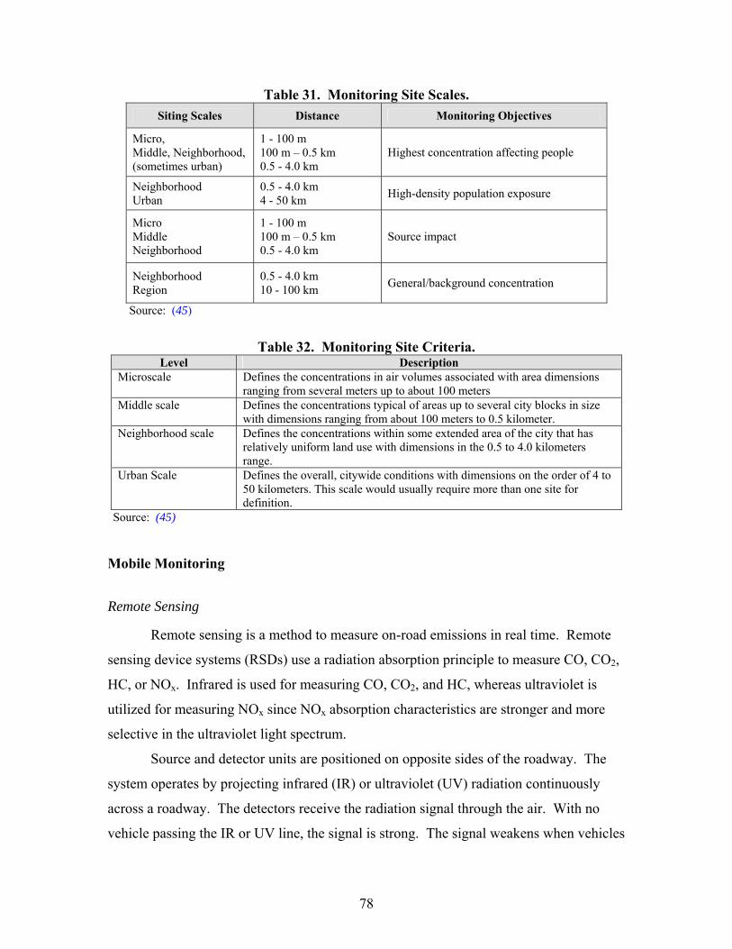
78
Table 31. Monitoring Site Scales. Siting Scales Distance Monitoring Objectives
Micro, Middle, Neighborhood, (sometimes urban)
1 - 100 m 100 m – 0.5 km 0.5 - 4.0 km
Highest concentration affecting people
Neighborhood Urban
0.5 - 4.0 km 4 - 50 km High-density population exposure
Micro Middle Neighborhood
1 - 100 m 100 m – 0.5 km 0.5 - 4.0 km
Source impact
Neighborhood Region
0.5 - 4.0 km 10 - 100 km General/background concentration
Source: (45)
Table 32. Monitoring Site Criteria. Level Description
Microscale Defines the concentrations in air volumes associated with area dimensions ranging from several meters up to about 100 meters
Middle scale
Defines the concentrations typical of areas up to several city blocks in size with dimensions ranging from about 100 meters to 0.5 kilometer.
Neighborhood scale
Defines the concentrations within some extended area of the city that has relatively uniform land use with dimensions in the 0.5 to 4.0 kilometers range.
Urban Scale Defines the overall, citywide conditions with dimensions on the order of 4 to 50 kilometers. This scale would usually require more than one site for definition.
Source: (45)
Mobile Monitoring
Remote Sensing
Remote sensing is a method to measure on-road emissions in real time. Remote
sensing device systems (RSDs) use a radiation absorption principle to measure CO, CO2,
HC, or NOx. Infrared is used for measuring CO, CO2, and HC, whereas ultraviolet is
utilized for measuring NOx since NOx absorption characteristics are stronger and more
selective in the ultraviolet light spectrum.
Source and detector units are positioned on opposite sides of the roadway. The
system operates by projecting infrared (IR) or ultraviolet (UV) radiation continuously
across a roadway. The detectors receive the radiation signal through the air. With no
vehicle passing the IR or UV line, the signal is strong. The signal weakens when vehicles
RESUBMITTAL
79
pass through the radiation stream. The amount of IR or UV light absorbed is related to
pollutants. RSDs with a freeze-frame video camera that can detect the license plate of
vehicles can store emissions information for each monitored vehicle, based on the license
plate number.
The uses of RSDs depend on the study purpose. RSDs should be an appropriate
emission measurement tool to capture the real-time emissions at a particular location,
such as ramps or intersections. However, it may be not an effective way to measure the
emission for the entire roadway, especially on freeways that have many lanes.
On-Board Emission Measurement
Another approach to measure on-road emissions is on-board emission
measurement. Unlike the snapshot measurements of RSDs, which can capture the
emissions only at a particular location, on-board emission measurement uses a “micro-
scale” approach to capture the on-road emissions in real time at any point of time and
location where the vehicle is driven. Real-time emissions can be measured for various
driving patterns (accelerations and decelerations), roadway geometry (grade and roadway
condition), driver behavior, etc. In addition, on-board emission measurement using a
micro-scale approach should be an effective method to evaluate the impacts of signal
improvements at intersections, which are too small to observe in a macroscopic model.
Also, the on-board emission measurement that can measure the real-time emission data
for actual driving conditions should prove advantageous over micro-scale modeling.
However, when continuous data are needed at a particular location, on-board emission
measurement may not be an effective method, especially for studying the trends of
emissions due to season and incident events (46).
Macroscopic Emission Models
The macroscopic modeling component consists of a model that has been
developed for freeway and arterial road networks for the whole region. Macroscopic
emission models, such as MOBILE6 (currently used in many states in United States) and
the California Air Resources Board’s (CARB) EMission FACtor (EMFAC) software
model (currently used in California) are commonly used to estimate the on-road
emissions in the United States. These models can predict gram per mile emissions of HC,
RESUBMITTAL
80
CO, NOx, CO2, PM, and toxics from cars, trucks, and motorcycles under various
conditions. MOBILE6 and EMFAC estimated composite emission rates are a function of
vehicle type and age, average speed, temperature, altitude, vehicle load, air conditioning
usage, and vehicle operating model. These models calculate region-wide emission factors
(EFs) in grams/mile for arterials, freeways, ramps, and other minor road connectors. The
emission rates can be combined with vehicle activities (VMT, number of trips, and
vehicle-hours traveled) from a travel demand model to develop highway emission
inventories expressed in tons per time period (46).
Microscopic Emission Models
Microscopic emission models are utilized to simulate traffic, such as freeway
segments, freeway on-ramps, intersections, etc. Second by second vehicle characteristics,
traffic conditions, and roadway conditions are required in order to obtain the emission
rates. Due to the ability to estimate the emissions second by second, microscopic
emission models are capable of assessing the impact of signal re-timing, modeling
roadway sections, etc. CORSIM is one of the microscopic emission models commonly
used to estimate on-road emissions. CORSIM applies emission rates from dynamometer
testing, summarized in speed and acceleration look-up tables, to estimate total roadway
emissions. Microscopic models are more accurate than region-wide macroscopic models
for evaluating micro-scale impacts, such as those of signal coordination, but may still be
inaccurate if not calibrated for local conditions. Also, vehicle operating history can
impact emissions, but speed-acceleration tables cannot account for this. Microscopic
models, however, represent the best strategy for estimating benefits prior to implementing
a micro-scale traffic improvement project (46).
EMISSION PERFORMANCE MEASURES
A good emission performance measure should be practical and realistic. It should
be easy for all people to understand and easy to develop with available data. Moreover, it
should be provided in time, so users, such as travelers or the government, still have time
to react to the air pollution condition. For example, an emission performance measure
such as AQI can provide air quality information along the roadway network so that
RESUBMITTAL
81
travelers will know the air quality condition and try to avoid routes with high air
pollutants. In addition, the DOTs can use emission performance measures to evaluate
project implementation and future funding allocations.
Since the initial realization that air pollution is a significant problem in parts of
the United. States, emission performance measures such as AQI and PSI, have been used
to assess the ambient air quality in many states and regions. Although the use of
indicators has been increasing, the definition and selection of emission performance
measures are still at an early stage. There are no exact rules for performance measure
selection. Criteria for choosing measures can be identified by the people who collect and
use the data or experts who understand the strength and limitation of each performance
measure. However, good performance measures should be a direct consequence of
activities. For example, emissions generated from roadways are defined as an outcome
measure. If the desired result is minimizing emissions, the emission rate should be a
good performance measure (direct consequence). A proxy measure may sometimes be
used in the absence of suitable performance measures due to time, budget constraints, or
unavailability of data. For example, when considering the desired result of emission
reductions, instead of using the direct outcome measure of emission rate, output
measures, such as the vehicle registration or congestion level, may serve as indirect
performance measures. Unfortunately, a proxy measure may not present a good result or
measure because the correlation may be weak. Consistency and data availability
sometimes limit the effectiveness of the performance measures.
Table 33 lists the typical emissions performance measures compiled from the
literature. In addition, the table identifies if the measure is qualitative or quantitative in
nature, as well as identifying the data needs for the calculation of the measure. Table 34
reduces this list to those measures which are appropriate for use in the transportation
arena. Table 34 also identifies whether the measure can be used in real time.
RESUBMITTAL
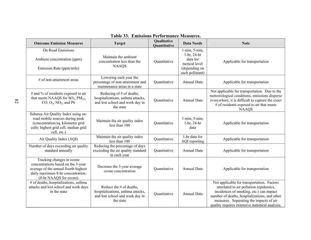
82
Table 33. Emissions Performance Measures. Outcome Emission Measures Target Qualitative
Quantitative Data Needs Note
On Road Emissions
Ambient concentration (ppm)
Emission Rate (ppm/mile)
Maintain the ambient concentration less than the
NAAQS Quantitative
1-min, 5-min, 1-hr, 24-hr
data for tactical level
(depending on each pollutant)
Applicable for transportation
# of non-attainment areas
Lowering each year the percentage of non-attainment and
maintenance areas in a state Quantitative Annual Data Applicable for transportation
# and % of residents exposed to air that meets NAAQS for SO2, PM25,
CO, O3, NO2, and Pb
Reducing of # of deaths, hospitalizations, asthma attacks, and lost school and work day in
the state
Quantitative Annual Data
Not applicable for transportation. Due to the meteorological conditions, emissions disperse everywhere; it is difficult to capture the exact
# of residents exposed to air that meets NAAQS
Subarea Air Quality Index using on-road mobile sources during peak (concentration/sq. kilometer grid
cells; highest grid cell, median grid cell, etc.)
Maintain the air quality index less than 100 Quantitative
1-min, 5-min, 1-hr, 24-hr
data Applicable for transportation
Air Quality Index (AQI) Maintain the air quality index less than 100 Quantitative 1-hr data for
AQI reporting Applicable for transportation
Number of days exceeding air quality standard annually
Reducing the percentage of days exceeding the air quality standard
in each year Quantitative Annual Data Applicable for transportation
Tracking changes in ozone concentrations based on the 3-year
average of the annual fourth highest daily maximum 8-hr concentration.
(8-hr NAAQS for ozone)
Decrease the 3-year average ozone concentration Quantitative Annual Data Applicable for transportation
# of deaths, hospitalizations, asthma attacks and lost school and work days
in the state Reduce the # of deaths,
hospitalizations, asthma attacks, and lost school and work day in
the state
Quantitative Annual Data
Not applicable for transportation. Factors unrelated to air pollution (epidemics,
incidences of smoking, etc.) can impact number of deaths, hospitalizations, and other
measures. Separating the impacts of air quality requires extensive statistical analysis.
RE
SU
BM
ITT
AL
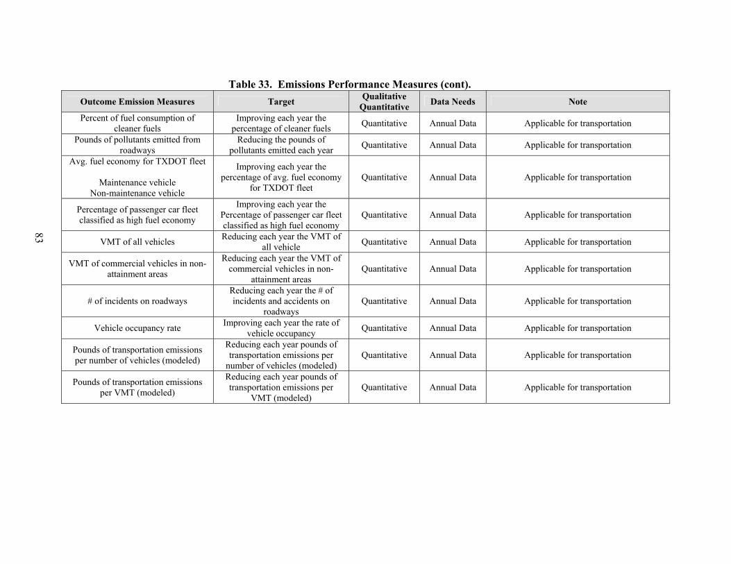
83
Table 33. Emissions Performance Measures (cont).
Outcome Emission Measures Target Qualitative Quantitative Data Needs Note
Percent of fuel consumption of cleaner fuels
Improving each year the percentage of cleaner fuels Quantitative Annual Data Applicable for transportation
Pounds of pollutants emitted from roadways
Reducing the pounds of pollutants emitted each year Quantitative Annual Data Applicable for transportation
Avg. fuel economy for TXDOT fleet
Maintenance vehicle Non-maintenance vehicle
Improving each year the percentage of avg. fuel economy
for TXDOT fleet Quantitative Annual Data Applicable for transportation
Percentage of passenger car fleet classified as high fuel economy
Improving each year the Percentage of passenger car fleet classified as high fuel economy
Quantitative Annual Data Applicable for transportation
VMT of all vehicles Reducing each year the VMT of all vehicle Quantitative Annual Data Applicable for transportation
VMT of commercial vehicles in non-attainment areas
Reducing each year the VMT of commercial vehicles in non-
attainment areas Quantitative Annual Data Applicable for transportation
# of incidents on roadways Reducing each year the # of incidents and accidents on
roadways Quantitative Annual Data Applicable for transportation
Vehicle occupancy rate Improving each year the rate of vehicle occupancy Quantitative Annual Data Applicable for transportation
Pounds of transportation emissions per number of vehicles (modeled)
Reducing each year pounds of transportation emissions per
number of vehicles (modeled) Quantitative Annual Data Applicable for transportation
Pounds of transportation emissions per VMT (modeled)
Reducing each year pounds of transportation emissions per
VMT (modeled) Quantitative Annual Data Applicable for transportation
RE
SU
BM
ITT
AL
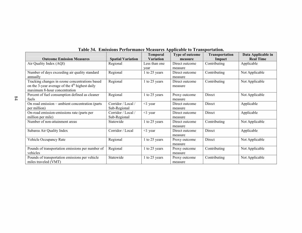
84
Table 34. Emissions Performance Measures Applicable to Transportation.
Outcome Emission Measures Spatial Variation Temporal Variation
Type of outcome measure
Transportation Impact
Data Applicable in Real Time
Air Quality Index (AQI) Regional Less than one year
Direct outcome measure
Contributing Applicable
Number of days exceeding air quality standard annually
Regional 1 to 25 years Direct outcome measure
Contributing Not Applicable
Tracking changes in ozone concentrations based on the 3-year average of the 4th highest daily maximum 8-hour concentration
Regional 1 to 25 years Direct outcome measure
Contributing Not Applicable
Percent of fuel consumption defined as cleaner fuels
Regional 1 to 25 years Proxy outcome measure
Direct Not Applicable
On road emission – ambient concentration (parts per million)
Corridor / Local / Sub-Regional
<1 year Direct outcome measure
Direct Applicable
On-road emission-emissions rate (parts per million per mile)
Corridor / Local / Sub-Regional
<1 year Direct outcome measure
Direct Applicable
Number of non-attainment areas Statewide 1 to 25 years Direct outcome measure
Contributing Not Applicable
Subarea Air Quality Index Corridor / Local <1 year Direct outcome measure
Direct Applicable
Vehicle Occupancy Rate Regional 1 to 25 years Proxy outcome measure
Direct Not Applicable
Pounds of transportation emissions per number of vehicles
Regional 1 to 25 years Proxy outcome measure
Contributing Not Applicable
Pounds of transportation emissions per vehicle miles traveled (VMT)
Statewide 1 to 25 years Proxy outcome measure
Contributing Not Applicable
RE
SU
BM
ITT
AL
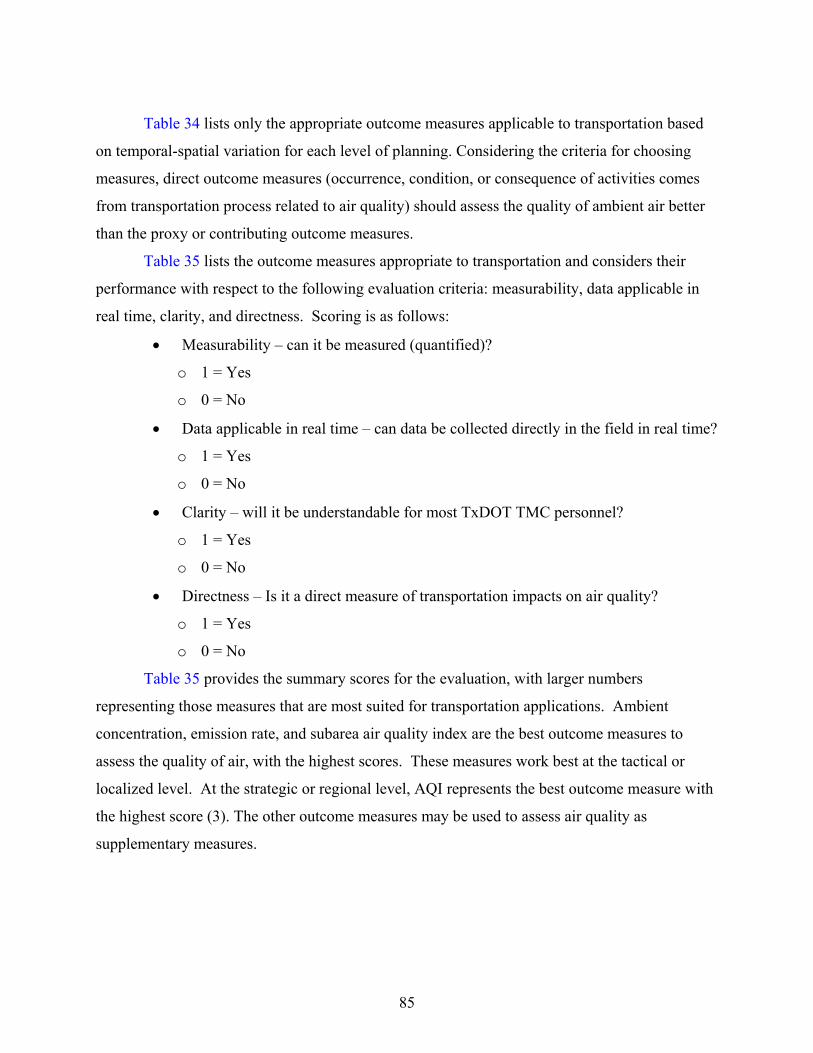
85
Table 34 lists only the appropriate outcome measures applicable to transportation based
on temporal-spatial variation for each level of planning. Considering the criteria for choosing
measures, direct outcome measures (occurrence, condition, or consequence of activities comes
from transportation process related to air quality) should assess the quality of ambient air better
than the proxy or contributing outcome measures.
Table 35 lists the outcome measures appropriate to transportation and considers their
performance with respect to the following evaluation criteria: measurability, data applicable in
real time, clarity, and directness. Scoring is as follows:
• Measurability – can it be measured (quantified)?
o 1 = Yes
o 0 = No
• Data applicable in real time – can data be collected directly in the field in real time?
o 1 = Yes
o 0 = No
• Clarity – will it be understandable for most TxDOT TMC personnel?
o 1 = Yes
o 0 = No
• Directness – Is it a direct measure of transportation impacts on air quality?
o 1 = Yes
o 0 = No
Table 35 provides the summary scores for the evaluation, with larger numbers
representing those measures that are most suited for transportation applications. Ambient
concentration, emission rate, and subarea air quality index are the best outcome measures to
assess the quality of air, with the highest scores. These measures work best at the tactical or
localized level. At the strategic or regional level, AQI represents the best outcome measure with
the highest score (3). The other outcome measures may be used to assess air quality as
supplementary measures.
RESUBMITTAL
86
Table 35. Evaluation of Emission Performance Measures Applicable to Transportation. Outcome Emission Measure Measurability Data Applicable In
Real Time Clarity Directness Total
On road emission - Ambient concentration (ppm) - Emission rate (ppm/mile)
4
Number of non-attainment areas 2 Subarea Air Quality Index 4 Air Quality Index (AQI) 3 Number of days exceeding air quality standard annually 2 Tracking changes in ozone concentrations based on the 3-year average of the annual fourth highest daily maximum 8-hour concentration. 1
Percent of fuel consumption defined as cleaner fuels 2 Average fuel economy for TXDOT fleet
- Maintenance veh. - Non-maintenance veh.
2
Percentage of passenger car fleet classified as high fuel economy 2 VMT of all vehicles 2 VMT of commercial vehicles in non-attainment areas
2
Number of incidents and accidents on roadway 2
Vehicle occupancy rate 2
Pounds of transportation emissions per number of vehicles (modeled) 2 Pounds of transportation emissions per VMT (modeled) 2
RE
SU
BM
ITT
AL
87
REFERENCES (1) Freeway Management and Operations Handbook. FHWA-OP-04-033. Federal Highway Administration, Washington, D.C., http://www.ops.fhwa.dot.gov/freewaymgmt/publications/frwy_mgmt_handbook/index.htm September 2003. (2) “Performance Measures of Operational Effectiveness for Highway Segments and Systems.” NCHRP Synthesis 311. Transportation Research Board, National Research Council, Washington, DC. http://www.trb.org/publications/nchrp/nchrp_syn_311.pdf 2003. (3) “Statisticians in History.” American Statistical Association. http://www.amstat.org/about/statisticians/index.cfm?fuseaction=biosinfo&BioID=4. Accessed April 9, 2006. (4) “The Deming Center History.” Deming Center. http://www.demingcenter.com/html_files/the_center/the_center_history.htm. Accessed April 9, 2006. (5) “Total Quality Management. An Overview.” HR Zone. http://www.hrzone.com/topics/tqm.html. Accessed March 11, 2005. (6) “The Philosophy of TQM. An Overview.” Course Notes for Engineering 401: Total Quality Management. Pat Hammett. University of Michigan. http://www.engin.umich.edu/class/eng401/003/LCNotes/phil.pdf. Accessed March 11, 2005. (7) “Serving The American Public: Best Practices in Performance Measurement” National Performance Review by Vice President Al Gore. June 1997. http://govinfo.library.unt.edu/npr/library/papers/benchmrk/nprbook.html. Accessed October 29, 2002. (8) “Performance Measurement in State Departments of Transportation.” NCHRP Synthesis 238. Transportation Research Board, National Research Council, Washington, DC, 1997. (9) “Highway Capacity Manual.” HCM 2000. Transportation Research Board, National Research Council, Washington, DC. 2000. (10) Lomax, Tim, and David Schrank. 2005 Urban Mobility Study. Texas Transportation Institute. May 2005. http://mobility.tamu.edu/ums/. Accessed March 1, 2006. (11) Stout, Thomas L., J.C. Liu., R. E. Brydia, and C. M. Poe. “TransLink Information Database Requirements.” Report to Texas Department of Transportation. TX-98/2988-2F. College Station, TX. October 1996.
RESUBMITTAL
88
(12) Turner, S.M., R.E. Brydia, J.C. Liu, and W.L. Eisele. “ITS Data Management System: Year One Activities,” Research Report 1752-2. Texas Transportation Institute, Texas A&M University, College Station, TX. August 1997. (13) Brydia, R. E., S. M. Turner, W. L. Eisele, and J.C. Liu. “Development of an ITS Data Management System.” Transportation Research Record 1625, Transportation Research Board, National Research Council. Washington, DC. 1998. pp. 124-130. (14) Roisman, Richard I., Ronald C. Welke, and Don Ostrander. The Montgomery County, Maryland, DASH System: Forecasting Future Traffic Volumes Using Real-Time Traffic Data. Compendium of Papers. Institute of Transportation Engineers. Nashville, TN. 2000. p.18. (15) Turner, Shawn M. Using ITS Data for Transportation System Performance Measurement. Conference Proceedings. “Traffic Congestion and Traffic Safety in the 21st Century: Challenges, Innovations, and Opportunities.” American Society of Civil Engineers, Chicago, IL. June 1997. pp. 340-346. (16) FHWA Office of Operations – About Operations. http://www.ops.fhwa.dot.gov/aboutus/aboutus.htm. Accessed April 15, 2006. (17) How to Measure Performance. A Handbook of Techniques and Tools. U.S. Department of Energy, Special Projects Group. Oak Ridge, TN. http://www.orau.gov/pbm/documents/handbook1a.html. October 1995. (18) A Guidebook for Performance-Based Transportation Planning. NCHRP Report 446. Transportation Research Board, National Research Council, Washington, DC. 2000. (19) Abbott, Eugene E., Joseph Cantalupo, and Linda B. Dixon. “Performance Measures. Linking Outputs and Outcomes to Achieve Goals.” Transportation Research Record 1617. Transportation Research Board, National Research Council, Washington, DC. 1998. pp. 90-95. (20) Pratt, Richard H., and Timothy J. Lomax. Performance Measures for Multimodal Transportation Systems. Transportation Research Record 1518. Transportation Research Board, National Research Council. Washington, DC. 1996. pp. 85-93. (21) Edward J. Seymour, James D. Carvell, Jr., Jodi L. Carson, Robert E. Brydia and James Paral. "Handbook for Developing a TMC Operations Manual" Report FHWA-HOP-06-015 .Federal Highway Administration. Washington, DC. November 2005. (22) “Guide to Effective Freeway Performance Measurement” NCHRP 3-86. Interim Report. National Cooperative Highway Research Program. Washington, DC. 2004. (23) National Transportation Operations Coalition (NTOC) Performance Measurement Initiative. Final Report. July 2005. http://www.ntoctalks.com/ntoc/ntoc_final_report.pdf Accessed multiple dates, April through September 2006.
RESUBMITTAL
89
(24) Boubel, R. W., D. L. Fox, D. B. Turner, and A. C. Stern. Fundamentals of Air Pollution., Academic Press. 1994. (25) EPA, Air Quality Index: A Guide to Air Quality and Your Health. August 2003. http://airnow.gov/index.cfm?action=aqibroch.index. (26) Henderson, Y., and Haggard, H. W., “Noxious Gases.” Chemical Catalog Co., New York, 1927; and U.S. Environmental Protection Agency, Research Triangle Park, NC; Air Quality Criteria for Carbon Monoxide EPA/ 600/8-90/045F. December 1991. (27) Goldsmith, J. R., and Frigerg, L. T. cited in Stern, A. C, Air pollution vol2; the effects of Air Pollution, Academic Press, Inc. 1977. (28) Sattler, M., Transportation and Air Quality Class Notes, University of Texas at Arlington, Arlington, TX. Fall 2005. (29) Cooper, C. D., and F. C. Alley. Air Pollution Control - A Design Approach, 3rd ed. Waveland Press, Prospect Heights, IL. 2002. (30) United States Environmental Protection Agency, Air Quality Trends, 1994. http://www.epa.gov:80/nceawww1/pdfs/0671ch05.pdf. Accessed multiple dates, July 2006. (31) Pope, C.A., III, Dockery, D. W., and Schwartz, J., Review of Epidemiological Evidence of Health Effects of Particulate Air Pollution, Inhalation Toxicology. July, 1995, pp. 1-18. (32) Air Quality Criteria for Particulate Matter and Sulfur Oxides, U.S. Environmental Protection Agency, Research Triangle Park, NC. http://cfpub.epa.gov/ncea/cfm/recordisplay.cfm?deid=46205. December 1981. (33) Review of the National Ambient Air Quality Standard for Particulate Matter: Assessment of Scientific and Technical Information, EPA-450/5-82-001. U.S. Environmental Protection Agency, Research 49 CFR § 50. July 1992. (34) Air Quality Criteria for Oxides of Nitrogen: Final Report U.S. Environmental Protection Agency, Research Triangle Park, NC. http://cfpub.epa.gov/ncea/cfm/recordisplay.cfm?deid=40179. 1983. (35) Review of the National Ambient Air Quality Standard for Nitrogen Dioxide, Assessment of Scientific and Technical Information, EPA-450/ 5-82-002. U.S. Environmental Protection Agency, Research Triangle Park, NC. March 1982. (36) Review of the National Ambient Air Quality Standards for Sulfur Oxides: Assessment of Scientific and Technical Information, Draft OAQPS Staff Paper, U.S. Environmental Protection Agency, Research Triangle Park, NC. April 1982.
RESUBMITTAL
90
(37) Air Quality Criteria for Ozone and Other Photochemical Oxidants, EPA 600/9-78-004. U.S. Environmental Protection Agency, Research Triangle Park, NC. April 1978. (38) Revisions to National Ambient Air Quality Standards for Photochemical Oxidants, Fed. Reg. Part V, 40 CFR § 50. July 1992. (39) United States Environmental Protection Agency. Green Book. Criteria Pollutants. http://earth1.epa.gov/air/oaqps/greenbk/o3co.html. Accessed multiple dates, July, 2006. (40) United States Environmental Protection Agency. Controlling Emissions During Episodes of High Air Pollution Potential. http://www.epa.gov/rgytgrnj/programs/artd/air/rules/missouri/10-6130.pdf. Accessed multiple times, July, 2006. (41) Stewart, C., T., Air Pollution, Human Health, and Public Policy, Lexington Books, 1979. (42) The UK National Air Quality Information Archive. http://www.airquality.co.uk/archive/standards.php#band. Accessed multiple times, July, 2006. (43) United States Environmental Protection Agency. National Ambient Air Monitoring Strategy Summary Document. http://www.epa.gov/ttn/amtic/files/ambient/monitorstrat/summary.pdf. Accessed multiple times, July, 2006. (44) Evans, G. F., T. A. Lumpkin, D. L. Smith, and M. C. Somerville. “Measurements of VOCs from the TAMS network,” J. Air Waste Mange. Assoc. 42, 1319-1323, (1992). (45) Texas Natural Resource Conservation Commission; TNRCC, Site Selection and Documentation Procedures Manual. July 1996. (46) Rupangi, P. M. Impacts of Signal Synchronization on Vehicular Emissions – An On-Board Measurement Case Study, M.S. thesis. University of Texas at Arlington. 2005.
RESUBMITTAL