On

Ma

b

a

ARRAA

KTAIL

1

ctittittaafm

tytu

1h

Applied Soft Computing 13 (2013) 1960–1968

Contents lists available at SciVerse ScienceDirect

Applied Soft Computing

j ourna l ho me p age: www.elsev ier .com/ l ocate /asoc

nline tool wear prediction system in the turning process using an adaptiveeuro-fuzzy inference system

uhammad Rizala,b, Jaharah A. Ghania,∗, Mohd Zaki Nuawia, Che Hassan Che Harona

Department of Mechanical and Materials Engineering, Faculty of Engineering and Built Environment, Universiti Kebangsaan Malaysia, 43600 Bangi, MalaysiaDepartment of Mechanical Engineering, Faculty of Engineering, Syiah Kuala University (UNSYIAH), 23111 Darussalam, Banda Aceh, Indonesia

r t i c l e i n f o

rticle history:eceived 22 February 2012eceived in revised form 30 May 2012ccepted 25 November 2012vailable online 12 December 2012

eywords:ool wear predictionNFIS

-kaz method

a b s t r a c t

Tool wear is a detrimental factor that affects the quality and tolerance of machined parts. Having anaccurate prediction of tool wear is important for machining industries to maintain the machined surfacequality and can consequently reduce inspection costs and increase productivity. Online and real-timetool wear prediction is possible due to developments in sensor technology. Recently, various sensors andmethods have been proposed for the development of tool wear monitoring systems. In this study, anonline tool wear monitoring system was proposed using a strain gauge-type sensor due to its simplicityand low cost. A model, based on the adaptive network-based fuzzy inference system (ANFIS), and anew statistical signal analysis method, the I-kaz method, were used to predict tool wear during a turningprocess. In order to develop the ANFIS model, the cutting speed, depth of cut, feed rate and I-kaz coefficient

ow-cost sensor from the signals of each turning process were taken as inputs, and the flank wear value for the cuttingedge was an output of the model. It was found that the prediction usually accurate if the correlationof coefficients and the average errors were in the range of 0.989–0.995 and 2.30–5.08% respectively forthe developed model. The proposed model is efficient and low-cost which can be used in the machiningindustry for online prediction of the cutting tool wear progression, but the accuracy of the model dependsupon the training and testing data.

. Introduction

Tool wear is an inevitable phenomenon in the machining pro-ess that is caused by the interaction between the cutting tool andhe machined workpiece. Tool wear progression needs to be mon-tored, and if the machining process continues with a worn tool,he worn tool can deteriorate the machined part quality, increasehe production time and cost, and even cause machine breakdownf the cutting tool suddenly fails. In practice, approximately 20% ofhe downtime in the machining processes is reported to be due toool failure, and the costs of cutting tools and their replacementccount for approximately 3–12% of total production costs [1,2]. Tovoid catastrophic tool failure, the progression of cutting tool wearrom the beginning of the cutting process should be predicted and

onitored in real-time.Many researchers have studied the tool wear prediction during

urning process with various sensors and methods in the past few

ears. Kaye et al. [3] proposed a technique for online prediction ofhe flank wear in turning using the change in spindle speed. Theysed a Bell Watt transducer to measure the changes in the three

∗ Corresponding author.E-mail address: jaharah@eng.ukm.my (J.A. Ghani).

568-4946/$ – see front matter © 2012 Elsevier B.V. All rights reserved.ttp://dx.doi.org/10.1016/j.asoc.2012.11.043

© 2012 Elsevier B.V. All rights reserved.

phase power consumption of the motor and developed predictivemodel based on empirical equation from sampled spindle speedpoints. Kopac and Sali [4] built a prediction model of tool wearfor a variety of different cutting speeds and feed rate using a con-denser microphone and analysed the frequency from 0 to 22 kHz.They found the tool wear increases by comparing the referencenoise with the noise during machining. Choudhury and Kishore [5]developed a method to predict flank wear on a cutting tool in tur-ning process using cutting force signals. The flank wear and the ratioof forces at different cutting conditions were collected experimen-tally to develop a mathematical model for predicting flank wear.Choudhury and Srinivas [6] also used index of diffusion, wear coef-ficient, rate of increase of normal load, and hardness of tool materialas input parameters to develop the mathematical model.

However, tool wear is a complex phenomenon and nonlinearproblem occurring due to various factors and ways. Therefore, deci-sion making support system is needed to determine the statusof tool wear during turning process. In the previous studies, sev-eral different approaches have been proposed to automate the toolwear prediction system. Ezugwu et al. [7] used an artificial neu-

ral network to predict tool wear based on experimental data andresulted in about 87.5% correct prediction. Lee et al. [8] applieda neural network to perform one step ahead prediction of flankwear from cutting force signals obtained from a tool dynamometer.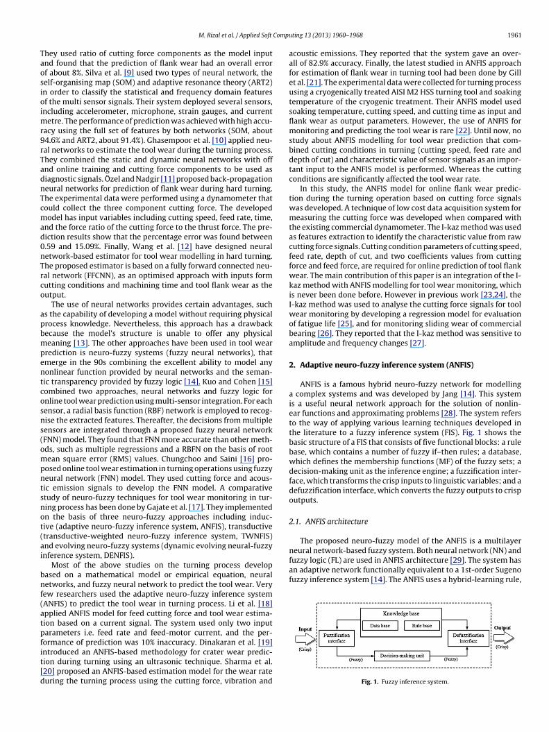

Compu

Taosioimr9rTadnTcmad0nTrco

apbmpentcosns(ompntsnot(ai

bnf(atpfit[d

neural network-based fuzzy system. Both neural network (NN) andfuzzy logic (FL) are used in ANFIS architecture [29]. The system hasan adaptive network functionally equivalent to a 1st-order Sugenofuzzy inference system [14]. The ANFIS uses a hybrid-learning rule,

M. Rizal et al. / Applied Soft

hey used ratio of cutting force components as the model inputnd found that the prediction of flank wear had an overall errorf about 8%. Silva et al. [9] used two types of neural network, theelf-organising map (SOM) and adaptive resonance theory (ART2)n order to classify the statistical and frequency domain featuresf the multi sensor signals. Their system deployed several sensors,ncluding accelerometer, microphone, strain gauges, and current

etre. The performance of prediction was achieved with high accu-acy using the full set of features by both networks (SOM, about4.6% and ART2, about 91.4%). Ghasempoor et al. [10] applied neu-al networks to estimate the tool wear during the turning process.hey combined the static and dynamic neural networks with offnd online training and cutting force components to be used asiagnostic signals. Özel and Nadgir [11] proposed back-propagationeural networks for prediction of flank wear during hard turning.he experimental data were performed using a dynamometer thatould collect the three component cutting force. The developedodel has input variables including cutting speed, feed rate, time,

nd the force ratio of the cutting force to the thrust force. The pre-iction results show that the percentage error was found between.59 and 15.09%. Finally, Wang et al. [12] have designed neuraletwork-based estimator for tool wear modelling in hard turning.he proposed estimator is based on a fully forward connected neu-al network (FFCNN), as an optimised approach with inputs formutting conditions and machining time and tool flank wear as theutput.

The use of neural networks provides certain advantages, suchs the capability of developing a model without requiring physicalrocess knowledge. Nevertheless, this approach has a drawbackecause the model’s structure is unable to offer any physicaleaning [13]. The other approaches have been used in tool wear

rediction is neuro-fuzzy systems (fuzzy neural networks), thatmerge in the 90s combining the excellent ability to model anyonlinear function provided by neural networks and the seman-ic transparency provided by fuzzy logic [14]. Kuo and Cohen [15]ombined two approaches, neural networks and fuzzy logic fornline tool wear prediction using multi-sensor integration. For eachensor, a radial basis function (RBF) network is employed to recog-ise the extracted features. Thereafter, the decisions from multipleensors are integrated through a proposed fuzzy neural networkFNN) model. They found that FNN more accurate than other meth-ds, such as multiple regressions and a RBFN on the basis of rootean square error (RMS) values. Chungchoo and Saini [16] pro-

osed online tool wear estimation in turning operations using fuzzyeural network (FNN) model. They used cutting force and acous-ic emission signals to develop the FNN model. A comparativetudy of neuro-fuzzy techniques for tool wear monitoring in tur-ing process has been done by Gajate et al. [17]. They implementedn the basis of three neuro-fuzzy approaches including induc-ive (adaptive neuro-fuzzy inference system, ANFIS), transductivetransductive-weighted neuro-fuzzy inference system, TWNFIS)nd evolving neuro-fuzzy systems (dynamic evolving neural-fuzzynference system, DENFIS).

Most of the above studies on the turning process developased on a mathematical model or empirical equation, neuraletworks, and fuzzy neural network to predict the tool wear. Very

ew researchers used the adaptive neuro-fuzzy inference systemANFIS) to predict the tool wear in turning process. Li et al. [18]pplied ANFIS model for feed cutting force and tool wear estima-ion based on a current signal. The system used only two inputarameters i.e. feed rate and feed-motor current, and the per-ormance of prediction was 10% inaccuracy. Dinakaran et al. [19]

ntroduced an ANFIS-based methodology for crater wear predic-ion during turning using an ultrasonic technique. Sharma et al.20] proposed an ANFIS-based estimation model for the wear rateuring the turning process using the cutting force, vibration and

ting 13 (2013) 1960–1968 1961

acoustic emissions. They reported that the system gave an over-all of 82.9% accuracy. Finally, the latest studied in ANFIS approachfor estimation of flank wear in turning tool had been done by Gillet al. [21]. The experimental data were collected for turning processusing a cryogenically treated AISI M2 HSS turning tool and soakingtemperature of the cryogenic treatment. Their ANFIS model usedsoaking temperature, cutting speed, and cutting time as input andflank wear as output parameters. However, the use of ANFIS formonitoring and predicting the tool wear is rare [22]. Until now, nostudy about ANFIS modelling for tool wear prediction that com-bined cutting conditions in turning (cutting speed, feed rate anddepth of cut) and characteristic value of sensor signals as an impor-tant input to the ANFIS model is performed. Whereas the cuttingconditions are significantly affected the tool wear rate.

In this study, the ANFIS model for online flank wear predic-tion during the turning operation based on cutting force signalswas developed. A technique of low cost data acquisition system formeasuring the cutting force was developed when compared withthe existing commercial dynamometer. The I-kaz method was usedas features extraction to identify the characteristic value from rawcutting force signals. Cutting condition parameters of cutting speed,feed rate, depth of cut, and two coefficients values from cuttingforce and feed force, are required for online prediction of tool flankwear. The main contribution of this paper is an integration of the I-kaz method with ANFIS modelling for tool wear monitoring, whichis never been done before. However in previous work [23,24], theI-kaz method was used to analyse the cutting force signals for toolwear monitoring by developing a regression model for evaluationof fatigue life [25], and for monitoring sliding wear of commercialbearing [26]. They reported that the I-kaz method was sensitive toamplitude and frequency changes [27].

2. Adaptive neuro-fuzzy inference system (ANFIS)

ANFIS is a famous hybrid neuro-fuzzy network for modellinga complex systems and was developed by Jang [14]. This systemis a useful neural network approach for the solution of nonlin-ear functions and approximating problems [28]. The system refersto the way of applying various learning techniques developed inthe literature to a fuzzy inference system (FIS). Fig. 1 shows thebasic structure of a FIS that consists of five functional blocks: a rulebase, which contains a number of fuzzy if–then rules; a database,which defines the membership functions (MF) of the fuzzy sets; adecision-making unit as the inference engine; a fuzzification inter-face, which transforms the crisp inputs to linguistic variables; and adefuzzification interface, which converts the fuzzy outputs to crispoutputs.

2.1. ANFIS architecture

The proposed neuro-fuzzy model of the ANFIS is a multilayer

Fig. 1. Fuzzy inference system.

1962 M. Rizal et al. / Applied Soft Computing 13 (2013) 1960–1968

NFIS a

wssrfnwhotttfu

tma

iptnt

O

O

wwbF�

�

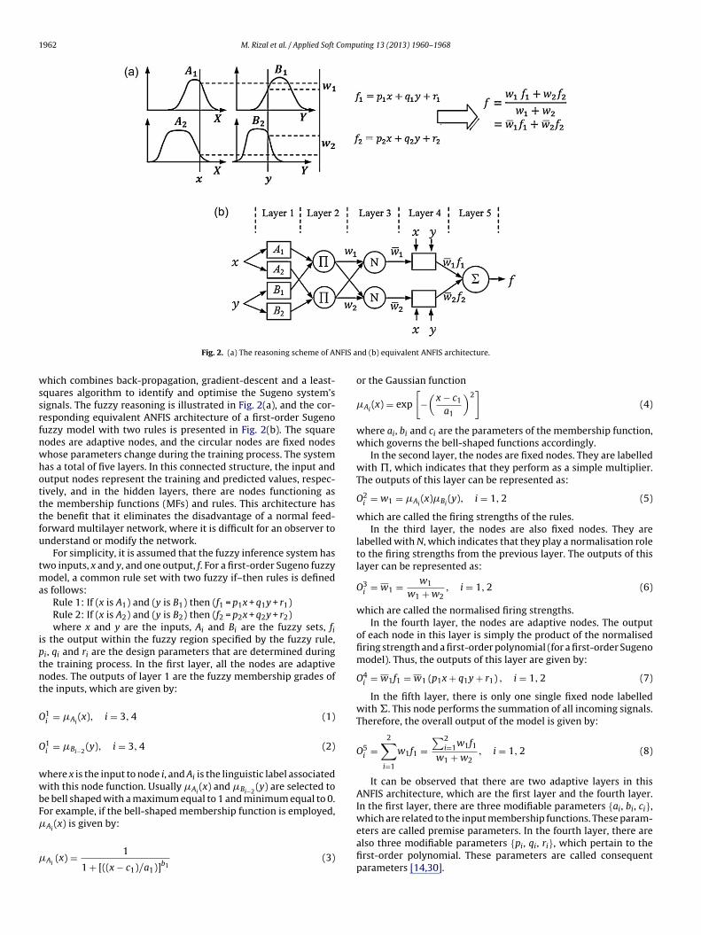
Fig. 2. (a) The reasoning scheme of A

hich combines back-propagation, gradient-descent and a least-quares algorithm to identify and optimise the Sugeno system’signals. The fuzzy reasoning is illustrated in Fig. 2(a), and the cor-esponding equivalent ANFIS architecture of a first-order Sugenouzzy model with two rules is presented in Fig. 2(b). The squareodes are adaptive nodes, and the circular nodes are fixed nodeshose parameters change during the training process. The systemas a total of five layers. In this connected structure, the input andutput nodes represent the training and predicted values, respec-ively, and in the hidden layers, there are nodes functioning ashe membership functions (MFs) and rules. This architecture hashe benefit that it eliminates the disadvantage of a normal feed-orward multilayer network, where it is difficult for an observer tonderstand or modify the network.

For simplicity, it is assumed that the fuzzy inference system haswo inputs, x and y, and one output, f. For a first-order Sugeno fuzzy

odel, a common rule set with two fuzzy if–then rules is defineds follows:

Rule 1: If (x is A1) and (y is B1) then (f1 = p1x + q1y + r1)Rule 2: If (x is A2) and (y is B2) then (f2 = p2x + q2y + r2)where x and y are the inputs, Ai and Bi are the fuzzy sets, fi

s the output within the fuzzy region specified by the fuzzy rule,i, qi and ri are the design parameters that are determined duringhe training process. In the first layer, all the nodes are adaptiveodes. The outputs of layer 1 are the fuzzy membership grades ofhe inputs, which are given by:

1i = �Ai

(x), i = 3, 4 (1)

1i = �Bi−2

(y), i = 3, 4 (2)

here x is the input to node i, and Ai is the linguistic label associatedith this node function. Usually �Ai

(x) and �Bi−2(y) are selected to

e bell shaped with a maximum equal to 1 and minimum equal to 0.or example, if the bell-shaped membership function is employed,

(x) is given by:

Ai

Ai(x) = 1

1 + [((x − c1)/a1)]b1(3)

nd (b) equivalent ANFIS architecture.

or the Gaussian function

�Ai(x) = exp

[−(

x − c1

a1

)2]

(4)

where ai, bi and ci are the parameters of the membership function,which governs the bell-shaped functions accordingly.

In the second layer, the nodes are fixed nodes. They are labelledwith �, which indicates that they perform as a simple multiplier.The outputs of this layer can be represented as:

O2i = w1 = �Ai

(x)�Bi(y), i = 1, 2 (5)

which are called the firing strengths of the rules.In the third layer, the nodes are also fixed nodes. They are

labelled with N, which indicates that they play a normalisation roleto the firing strengths from the previous layer. The outputs of thislayer can be represented as:

O3i = w1 = w1

w1 + w2, i = 1, 2 (6)

which are called the normalised firing strengths.In the fourth layer, the nodes are adaptive nodes. The output

of each node in this layer is simply the product of the normalisedfiring strength and a first-order polynomial (for a first-order Sugenomodel). Thus, the outputs of this layer are given by:

O4i = w1f1 = w1 (p1x + q1y + r1) , i = 1, 2 (7)

In the fifth layer, there is only one single fixed node labelledwith �. This node performs the summation of all incoming signals.Therefore, the overall output of the model is given by:

O5i =

2∑i=1

w1f1 =∑2

i=1w1f1w1 + w2

, i = 1, 2 (8)

It can be observed that there are two adaptive layers in thisANFIS architecture, which are the first layer and the fourth layer.In the first layer, there are three modifiable parameters {ai, bi, ci},which are related to the input membership functions. These param-

eters are called premise parameters. In the fourth layer, there arealso three modifiable parameters {pi, qi, ri}, which pertain to thefirst-order polynomial. These parameters are called consequentparameters [14,30].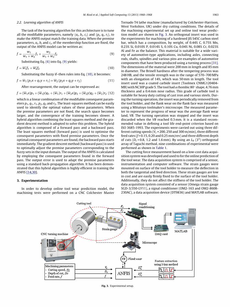

Compu

2

ampo

f

f

f

f

weutlhdaTcoitfbpusA

3

m

M. Rizal et al. / Applied Soft

.2. Learning algorithm of ANFIS

The task of the learning algorithm for this architecture is to tunell the modifiable parameters, namely {ai, bi, ci} and {pi, qi, ri}, toake the ANFIS output match the training data. When the premise

arameters, ai, bi and ci, of the membership function are fixed, theutput of the ANFIS model can be written as:

= w1

w1 + w2f1 + w2

w1 + w2f2 (9)

Substituting Eq. (6) into Eq. (9) yields:

= w1f1 + w2f2 (10)

Substituting the fuzzy if–then rules into Eq. (10), it becomes:

= w1 (p1x + q1y + r1) + w2 (p2x + q2y + r2) (11)

After rearrangement, the output can be expressed as:

= (w1x)p1 + (w1y)q1 + (w1)r1 + (w2x)p2 + (w2y)q2 + (w2)r2 (12)

hich is a linear combination of the modifiable consequent param-ters p1, q1, r1, p2, q2 and r2. The least-squares method can be easilysed to identify the optimal values of these parameters. Whenhe premise parameters are not fixed, the search space becomesarger, and the convergence of the training becomes slower. Aybrid algorithm combining the least squares method and the gra-ient descent method is adopted to solve this problem. The hybridlgorithm is composed of a forward pass and a backward pass.he least squares method (forward pass) is used to optimise theonsequent parameters with fixed premise parameters. Once theptimal consequent parameters are found, the backward pass startsmmediately. The gradient descent method (backward pass) is usedo optimally adjust the premise parameters corresponding to theuzzy sets in the input domain. The output of the ANFIS is calculatedy employing the consequent parameters found in the forwardass. The output error is used to adapt the premise parameterssing a standard back-propagation algorithm. It has been demon-trated that this hybrid algorithm is highly efficient in training theNFIS [14,30].

. Experimentation

In order to develop online tool wear prediction model, theachining tests were performed on a CNC Colchester Master

Fig. 3. Experime

ting 13 (2013) 1960–1968 1963

Tornado T4 lathe machine (manufactured by Colchester-Harrison,West Yorkshire, UK) under dry cutting conditions. The details ofthe machining experimental set up and online tool wear predic-tion model are shown in Fig. 3. An orthogonal insert was used inthe experiments for machining of a hardened JIS S45C carbon steelbar, which has a composition, by weight, of 0.44% C, 0.75% Mn,0.23% Si, 0.010% P, 0.014% S, 0.10% Cu, 0.04% Ni, 0.08% Cr, 0.023%Al and Fe as the balance. This material is suitable for a wide vari-ety of automotive-type applications, including axles, connectingrods, shafts, spindles and various pins are examples of automotivecomponents that have been produced using a turning process [31].The dimensions of the material were 200 mm in length and 85 mmin diameter. The Brinell hardness after the tempering process was248 HB, and the tensile strength was in the range of 570–700 MPawith an elongation of 14%, which was 50 mm in length. The toolinsert used was a coated carbide insert (Toolmex CNMG120404-MB) with NC30P grade 5. The tool had a rhombic 80◦ shape, 4.76 mmthickness and a 0.4 mm nose radius. This grade of carbide tool issuitable for heavy duty cutting of cast iron and various steels. Dur-ing the turning operation, the insert was periodically removed fromthe tool holder, and the flank wear on the flank face was measuredusing a Mitutoyo toolmaker’s microscope. The measured parame-ter to represent the progress of wear was the average flank wearland, VB. The turning operation was stopped and the insert wasdiscarded when the VB reached 0.3 mm. It is a standard recom-mended value in defining a tool life end-point criterion based onISO 3685-1993. The experiments were carried out using three dif-ferent cutting speeds (Vc = 200, 250 and 300 m/min), three differentfeed rates (f = 0.15, 0.20 and 0.25 mm/rev) and three different depthof cuts (Dc = 0.8, 1.2 and 1.6 mm). By using an L9 (33) orthogonalarray of Taguchi method, nine combinations of experimental wereperformed as shown in Table 1.

The cutting force measurement based on a low-cost data acqui-sition system was developed and used to for the online prediction ofthe tool wear. The data acquisition system is comprised of a sensor,instrumentation and computer software. The strain gauges weremounted on surface of the tool holder to measure the deflection inboth the tangential and feed direction. These strain gauges are lowin cost and are easily firmly fixed to the surface of the tool holder.

Additionally, they do not affect the stiffness of the tool holder. Thedata acquisition system consisted of a sensor (Omega strain gaugeSGD-3/350-LY11), a signal conditioner (OM2-163 and OM2-8608-230AC), a data acquisition device (DT9836) and MATLAB software.

ntal setup.

1964 M. Rizal et al. / Applied Soft Compu

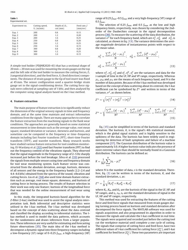
Table 1Experimental set.

Experiment no. Cutting speed,Vc (m/min)

Depth of, Dc ,cut (mm)

Feed rate, f(mm/rev)

Exp. 1 200 0.8 0.15Exp. 2 200 1.2 0.20Exp. 3 200 1.6 0.25Exp. 4 250 0.8 0.20Exp. 5 250 1.2 0.25Exp. 6 250 1.6 0.15Exp. 7 300 0.8 0.20Exp. 8 300 1.2 0.25

A2a(nagnt

4

tdctcmssdthiotitfso4ctcttA

Zpubakftfda

cut the workpiece material until complete a one cycle of cutting.

Exp. 9 300 1.6 0.15

simple tool holder (PDJNR2020-43) that has a sectional shape of0 mm × 20 mm was used for mounting the strain gauges on the topnd the left side of the tool holder to measure the cutting forces, Fc

tangential direction), and the feed force, Ff (feed direction) compo-ents. The distance of strain gauge to the tip of tool insert was fixedt 45 mm. The sensor configuration used a quarter-bridge strainauge set in the signal-conditioning device. The cutting force sig-als were collected at sampling rate of 1 kHz, and then analysed byhe computer using signal analysis based on the I-kaz method.

. Feature extraction

The main purpose of feature extraction is to significantly reducehe dimension of the original sensory signals in time and frequencyomain, and at the same time maintain and extract informationonditions from the signals. There are many approaches to correlatehe feature extraction from the machining signals to the flank wearonditions. The approaches are generally based on some statisticaleasurement in time domain such as the average value, root mean

quare, standard deviation or variance, skewness and kurtosis, andometime can be computed in the frequency or time–frequencyomain including fast Fourier transform (FFT), short-time Fourierransform (STFT), and wavelet transform. Many research worksave studied various feature extraction for tool condition monitor-

ng. El-Wardany et al. [32] used fast Fourier transform (FFT) to findut the frequency content of the vibrations signals. They observedhat the signal magnitude in the frequency range of 2–5 Hz sharplyncreased just before the tool breakage. Silva et al. [33] processedhe signals from multiple sensors using time and frequency domainor tool wear monitoring system. Each feature vector was con-tructed from the absolute deviation, average, kurtosis, skewnessf all sensors and the energy in the frequency bands (2.2–2.4 and.4–4.6 kHz) obtained from the spectra of the sound, vibration andutting forces. Liu et al. [34] also used time domain feature extrac-ion such as average, root mean square, skewness, and kurtosis ofutting force in boring process. The results of feature selection inheir work was only one feature; kurtosis of the longitudinal forcehat was needed for the online measurement of tool wear usingNFIS.

In this study, the integrated kurtosis-based algorithm for the-filter (I-kaz) method was used to assist the signal analysis inter-retation task. Both inferential and descriptive statistics weretilised in the I-kaz method. The I-kaz method was developedased on the concept of data scattering about the data centroidnd classified the display according to inferential statistics. The I-az method is used to model the data patterns, which accountsor the randomness and draws inferences from a larger popula-ion. These inferences are very useful for estimating and forecasting

uture observations [35]. The main idea of the I-kaz method isecompose a dynamic signal into three frequency ranges including

low-frequency (LF) range of 0–0.25 fmax, a high-frequency (HF)

ting 13 (2013) 1960–1968

range of 0.25 fmax–0.5 fmax and a very high-frequency (VF) range of0.5 fmax.

The selection of 0.25 fmax and 0.5 fmax as the low and highfrequency limits, respectively, was chosen by considering the 2nd-order of the Daubechies concept in the signal decompositionprocess [36]. To measure the scattering of the data distribution, thevariance �2 for each frequency band, which are �2

L , �2H and �2

V , iscalculated, as shown in Eq. (13). The variance determines the aver-age magnitude deviation of instantaneous points with respect tothe mean value.

�2L =

∑Ni=1

(xL

i− �L

)2

N; �2

H =∑N

i=1

(xH

i− �H

)2

N;

�2V =

∑Ni=1

(xV

i− �V

)2

N(13)

where �2L , �2

H, �2V and xL

i, xH

i, xV

iare the variances and data for the

i-sample of time in the LF, HF and VF range, respectively. Whereas�L, �H and �V are the means of each frequency band, and N is thenumber of data points. Because of the I-kaz method was developedbased on the concept of data scattering about its centroid, the I-kazcoefficient can be symbolised by Z∞ and written in terms of thevariance, �2, as shown below.

Z∞ =√

(�2L )

2 + (�2H)

2 + (�2V )

2(14)

Z∞ =

√∑Ni=1

(xL

i− �L

)4

N2+

∑Ni=1

(xH

i− �H

)4

N2+

∑Ni=1

(xV

i− �V

)4

N2

(15)

Eq. (15) can be simplified in terms of the kurtosis and standarddeviation. The kurtosis, K, is the signal’s 4th statistical moment,which is the global signal statistic and is highly sensitive to thespikiness of the data. The kurtosis has been widely used in engi-neering for detection of fault symptoms and failure of a machinecomponent [37]. The Gaussian distribution of the kurtosis value isapproximately 3.0. A higher kurtosis value indicates the presence ofmore extreme values than should be normally found in a Gaussiandistribution. The kurtosis can be defined as:

K = 1Ns4

N∑i=1

(xi − �)4 (16)

where N is the number of data, s is the standard deviation. There-fore, Eq. (3) can be written in terms of the kurtosis, K, and thestandard deviation, s, as:

Z∞ = 1N

√KLs4

L + KHs4H + KV s4

V (17)

where KL, KH, and KV are the kurtosis of the signal in the LF, HF andVF ranges, and sL, sH, sV are the standard deviations of signal in theLF, HF and VF ranges, respectively.

This method was used for extracting the features of the cuttingforce and feed force signals that measured from strain gauges dur-ing turning process based on kurtosis and standard deviation afterdecomposed the force signals. The MATLAB software was used forsignals acquisition and also programmed its algorithm in order tomeasure the signals and calculate the I-kaz coefficient in real time.The signals were acquired and recorded just before the cutting tool

The signals that comprise of cutting force and feed force, have twodifferent values of I-kaz coefficient for cutting force (Z∞

Fc), and I-kaz

coefficient for feed force (Z∞Ff

). These two parameters are important

Compu

iic

5

ihsf

ot1

(

apttctdfut

8ttactI

M. Rizal et al. / Applied Soft

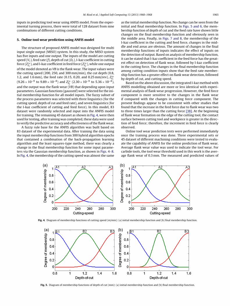
nputs in predicting tool wear using ANFIS model. From the exper-mental turning process, there were total of 128 dataset from nineombinations of different cutting conditions.

. Online tool wear prediction using ANFIS model

The structure of proposed ANFIS model was designed for multinput single output (MISO) system. In this study, the MISO systemas five inputs and one output. The inputs of the model are cuttingpeed (Vc), feed rate (f), depth of cut (Dc), I-kaz coefficient in cuttingorce (Z∞

Fc), and I-kaz coefficient in feed force (Z∞

Ff), while one output

f the model denoted as VB is the flank wear. The input values werehe cutting speed (200, 250, and 300 mm/min), the cut depth (0.8,.2, and 1.6 mm), the feed rate (0.15, 0.20, and 0.25 mm/rev), Z∞

Fc

9.26 × 10−9 to 9.89 × 10−8) and Z∞Ff

(2.30 × 10−9 to 5.36 × 10−8),

nd the output was the flank wear (VB) that depending upon inputarameters. Gaussian functions (gaussmf) were selected for the ini-ial membership function for all model inputs. The fuzzy subset ofhe process parameters was selected with three linguistics (for theutting speed, depth of cut and feed rate), and seven linguistics (forhe I-kaz coefficient of cutting and feed force). In this model, 83ataset were randomly selected and input into the ANFIS modelor training. The remaining 45 dataset as shown in Fig. 4, were thensed for testing, after training was completed, these data were usedo verify the predictive accuracy and effectiveness of the flank wear.

A fuzzy rule base for the ANFIS algorithm was built based on3 dataset of the experimental data. After training the data usinghe input membership functions from 300 hybrid algorithm epochshat contained a combination of the back-propagation learning

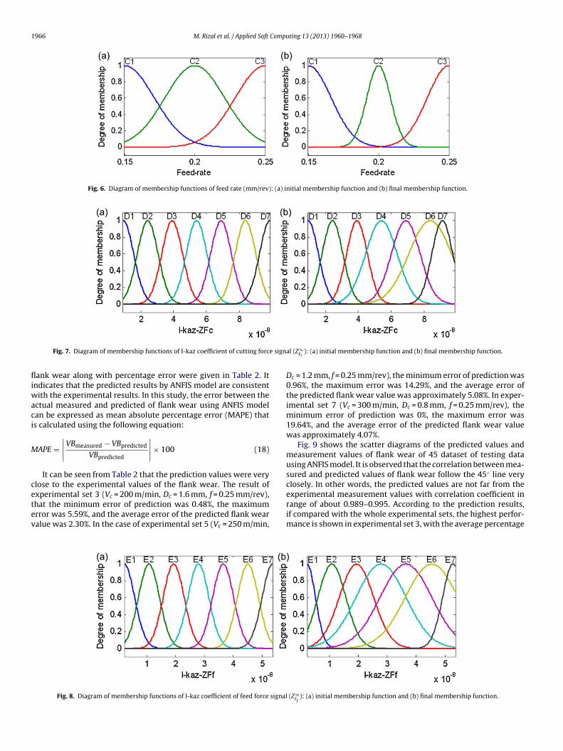
lgorithm and the least squares-type method, there was clearly ahange in the final membership function for some input parame-ers via the Gaussian membership function, as shown in Figs. 4–8.n Fig. 4, the membership of the cutting speed was almost the same

Fig. 4. Diagram of membership functions of cutting speed (m/min): (a)

Fig. 5. Diagram of membership functions of depth of cut (mm): (a) in

ting 13 (2013) 1960–1968 1965

as the initial membership function. No change can be seen from theinitial and final membership function. In Figs. 5 and 6, the mem-bership function of depth of cut and the feed rate have shown littlechanges on the final membership function and obviously seen inthe middle area. Finally, in Figs. 7 and 8, the membership of theI-kaz coefficient in the cutting and feed force, changes in the mid-dle and end areas are obvious. The amount of changes in the finalmembership functions of inputs indicates the effect of inputs onthe detection of output. Based on analysis of membership function,it can be stated that I-kaz coefficient in the feed force has the great-est effect on detection of flank wear, followed by I-kaz coefficientin the cutting force. The changes in the final membership functionamong cutting condition inputs show that the feed rate member-ship function has a greater effect on flank wear detection, followedby depth of cut, and cutting speed.

Based on the above discussion, the integrated I-kaz method withANFIS modelling obtained are more or less identical with experi-mental analysis of flank wear progression. However, the feed forcecomponent is more sensitive to the changes in the flank wearif compared with the changes in cutting force component. Thepresent findings appear to be consistent with other studies thatfound that the increase in the feed force due to flank wear was twoto three times larger than the cutting force [38]. At the beginningof flank wear formation on the edge of the cutting tool, the contactsurface between cutting tool and workpiece is greater in the direc-tion of feed force; therefore, the increment in feed force is clearlyobserved.

Online tool wear prediction tests were performed immediatelyonce the training process was done. Three experimental sets or45 dataset of different machining conditions were tested to evalu-

ate the capability of ANFIS for the online prediction of flank wear.Average flank wear value was used to indicate the tool wear. Forcarbide tools, the tool wear threshold used in this work is the aver-age flank wear of 0.3 mm. The measured and predicted values of

initial membership function and (b) final membership function.

itial membership function and (b) final membership function.

1966 M. Rizal et al. / Applied Soft Computing 13 (2013) 1960–1968

Fig. 6. Diagram of membership functions of feed rate (mm/rev): (a) initial membership function and (b) final membership function.

e sign

fliwaci

M

cetev

Fig. 7. Diagram of membership functions of I-kaz coefficient of cutting forc

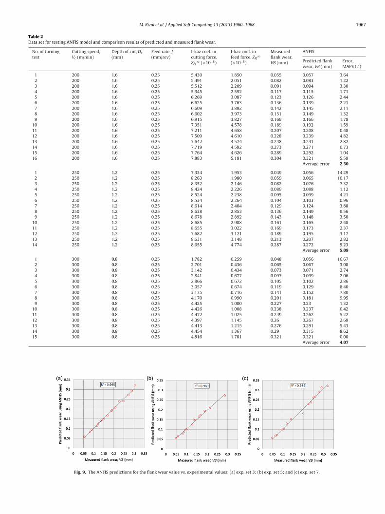
ank wear along with percentage error were given in Table 2. Itndicates that the predicted results by ANFIS model are consistent

ith the experimental results. In this study, the error between thectual measured and predicted of flank wear using ANFIS modelan be expressed as mean absolute percentage error (MAPE) thats calculated using the following equation:

APE =∣∣∣∣VBmeasured − VBpredicted

VBpredicted

∣∣∣∣ × 100 (18)

It can be seen from Table 2 that the prediction values were verylose to the experimental values of the flank wear. The result of

xperimental set 3 (Vc = 200 m/min, Dc = 1.6 mm, f = 0.25 mm/rev),hat the minimum error of prediction was 0.48%, the maximumrror was 5.59%, and the average error of the predicted flank wearalue was 2.30%. In the case of experimental set 5 (Vc = 250 m/min,

Fig. 8. Diagram of membership functions of I-kaz coefficient of feed force signal

al (Z∞Fc

): (a) initial membership function and (b) final membership function.

Dc = 1.2 mm, f = 0.25 mm/rev), the minimum error of prediction was0.96%, the maximum error was 14.29%, and the average error ofthe predicted flank wear value was approximately 5.08%. In exper-imental set 7 (Vc = 300 m/min, Dc = 0.8 mm, f = 0.25 mm/rev), theminimum error of prediction was 0%, the maximum error was19.64%, and the average error of the predicted flank wear valuewas approximately 4.07%.

Fig. 9 shows the scatter diagrams of the predicted values andmeasurement values of flank wear of 45 dataset of testing datausing ANFIS model. It is observed that the correlation between mea-sured and predicted values of flank wear follow the 45◦ line veryclosely. In other words, the predicted values are not far from the

experimental measurement values with correlation coefficient inrange of about 0.989–0.995. According to the prediction results,if compared with the whole experimental sets, the highest perfor-mance is shown in experimental set 3, with the average percentage

(Z∞Ff

): (a) initial membership function and (b) final membership function.

M. Rizal et al. / Applied Soft Computing 13 (2013) 1960–1968 1967

Table 2Data set for testing ANFIS model and comparison results of predicted and measured flank wear.

No. of turningtest

Cutting speed,Vc (m/min)

Depth of cut, Dc

(mm)Feed rate, f(mm/rev)

I-kaz coef. incutting force,ZFc

∞ (×10−8)

I-kaz coef. infeed force, ZFf

∞

(×10−8)

Measuredflank wear,VB (mm)

ANFIS

Predicted flankwear, VB (mm)

Error,MAPE (%)

1 200 1.6 0.25 5.430 1.850 0.055 0.057 3.642 200 1.6 0.25 5.491 2.051 0.082 0.083 1.223 200 1.6 0.25 5.512 2.209 0.091 0.094 3.304 200 1.6 0.25 5.945 2.592 0.117 0.115 1.715 200 1.6 0.25 6.269 3.087 0.123 0.126 2.446 200 1.6 0.25 6.625 3.763 0.136 0.139 2.217 200 1.6 0.25 6.609 3.892 0.142 0.145 2.118 200 1.6 0.25 6.602 3.973 0.151 0.149 1.329 200 1.6 0.25 6.915 3.827 0.169 0.166 1.78

10 200 1.6 0.25 7.351 4.578 0.189 0.192 1.5911 200 1.6 0.25 7.211 4.658 0.207 0.208 0.4812 200 1.6 0.25 7.509 4.610 0.228 0.239 4.8213 200 1.6 0.25 7.642 4.574 0.248 0.241 2.8214 200 1.6 0.25 7.719 4.592 0.273 0.271 0.7315 200 1.6 0.25 7.764 4.626 0.289 0.292 1.0416 200 1.6 0.25 7.883 5.181 0.304 0.321 5.59

Average error 2.30

1 250 1.2 0.25 7.334 1.953 0.049 0.056 14.292 250 1.2 0.25 8.263 1.980 0.059 0.065 10.173 250 1.2 0.25 8.352 2.146 0.082 0.076 7.324 250 1.2 0.25 8.424 2.226 0.089 0.088 1.125 250 1.2 0.25 8.524 2.238 0.095 0.099 4.216 250 1.2 0.25 8.534 2.264 0.104 0.103 0.967 250 1.2 0.25 8.614 2.404 0.129 0.124 3.888 250 1.2 0.25 8.638 2.853 0.136 0.149 9.569 250 1.2 0.25 8.678 2.892 0.143 0.148 3.50

10 250 1.2 0.25 8.685 2.988 0.161 0.165 2.4811 250 1.2 0.25 8.655 3.022 0.169 0.173 2.3712 250 1.2 0.25 7.682 3.121 0.189 0.195 3.1713 250 1.2 0.25 8.631 3.148 0.213 0.207 2.8214 250 1.2 0.25 8.655 4.774 0.287 0.272 5.23

Average error 5.08

1 300 0.8 0.25 1.782 0.259 0.048 0.056 16.672 300 0.8 0.25 2.701 0.436 0.065 0.067 3.083 300 0.8 0.25 3.142 0.434 0.073 0.071 2.744 300 0.8 0.25 2.841 0.677 0.097 0.099 2.065 300 0.8 0.25 2.866 0.672 0.105 0.102 2.866 300 0.8 0.25 3.057 0.674 0.119 0.129 8.407 300 0.8 0.25 3.175 0.716 0.141 0.152 7.808 300 0.8 0.25 4.170 0.990 0.201 0.181 9.959 300 0.8 0.25 4.425 1.000 0.227 0.23 1.32

10 300 0.8 0.25 4.426 1.008 0.238 0.237 0.4211 300 0.8 0.25 4.472 1.025 0.249 0.262 5.2212 300 0.8 0.25 4.397 1.145 0.26 0.267 2.6913 300 0.8 0.25 4.413 1.215 0.276 0.291 5.4314 300 0.8 0.25 4.454 1.367 0.29 0.315 8.6215 300 0.8 0.25 4.816 1.781 0.321 0.321 0.00

Average error 4.07

Fig. 9. The ANFIS predictions for the flank wear value vs. experimental values: (a) exp. set 3; (b) exp. set 5; and (c) exp. set 7.

1 Compu

eodw9ez

Icbpsfsgd

6

pdtfuwitccpfbtma5tei

A

(p

R

[

[

[

[

[

[

[

[

[

[

[

[

[

[

[

[

[

[

[

[

[

[

[

[

[

[

[

968 M. Rizal et al. / Applied Soft

rror only 2.30%. However, the variation in this prediction dependsn the testing dataset, which was not introduced to the ANFISuring the training process. These results indicate that the flankear prediction is reliable, and the accuracy is in the range of

5.93–97.70%. Theoretically, the prediction model is accepted asxcellent if the mean absolute percentage errors were proximity toero and accuracy closely to 100%.

These results demonstrate that the ANFIS model by using the-kaz method to extract the characteristic values from the signals,an excellently predict the flank wear. The ANFIS model can alsoe used for investigating the effects of the input parameters on theerformance parameters of the system. Therefore, the proposedystem is better and more economical in data acquisition systemor predicting the actual flank wear during the turning process. Theystem can be used in the machining industry to predict the pro-ression of cutting tool wear online, but the accuracy of the modelepends upon the training and testing data.

. Conclusions

The ANFIS with multi inputs fuzzy model was developed toredict the flank wear during turning process. The inputs of theeveloped model are cutting parameters of turning process (cut-ing speed, feed rate, depth of cut), and I-kaz coefficient for cuttingorce and feed force. The cutting force components were measuredsing in-house developed strain gauge sensor. The I-kaz methodas developed based on the decomposed frequency signals, and

ntegrated kurtosis-based algorithm was used to extract the fea-ures of the cutting force and feed force signals. The changes ofutting force signals due to flank wear were indicated by signifi-ant increasing the I-kaz coefficient values. Among the five inputarameters of ANFIS model, changes of the I-kaz coefficient in feedorce have the most effect on predicting flank wear value, followedy I-kaz coefficient in cutting force, feed rate, depth of cut, and cut-ing speed. It was found that the results generated by the ANFIS

odel are close to the experimental results with the minimumnd maximum average error of the flank wear of about 2.30% and.08% respectively. The accuracy of the prediction may achieve upo 95.93–97.70%. The performance of the prediction shows that thestimated results are very accurate and encouraging to be appliedn real industry application.

cknowledgements

The authors would like to thank the Government of MalaysiaMOSTI) and Universiti Kebangsaan Malaysia for their financial sup-ort under Grants 03-01-02-SF0647 and UKM-DLP-2011-057.

eferences

[1] S. Kurada, C. Bradley, A review of machine vision sensors for tool conditionmonitoring, Computer in Industry 34 (1997) 55–72.

[2] M. Castejon, E. Alegre, J. Barreiro, L.K. Hernandez, On-line tool wear monitor-ing using geometric descriptors from digital images, International Journal ofMachine Tools and Manufacture 47 (2007) 1847–1853.

[3] J.E. Kaye, D.-H. Yan, N. Popplewell, S. Balakrishnan, Predicting tool flank wearusing spindle speed change, International Journal of Machine Tools and Man-ufacture 35 (1995) 1309–1320.

[4] J. Kopac, S. Sali, Tool wear monitoring during the turning process, Journal ofMaterials Processing Technology 113 (2001) 312–316.

[5] S.K. Choudhury, K.K. Kishore, Tool wear measurement in turning using forceratio, International Journal of Machine Tools and Manufacture 40 (2000)899–909.

[6] S.K. Choudhury, P. Srinivas, Tool wear prediction in turning, Journal of Materials

Processing Technology 153–154 (2004) 276–280.

[7] E.O. Ezugwu, S.J. Arthur, E.L. Hines, Tool-wear prediction using artificial neuralnetworks, Journal of Materials Processing Technology 49 (1995) 255–264.

[8] J.H. Lee, D.E. Kim, S.J. Lee, Application of neural networks to flank wear predic-tion, Mechanical Systems and Signal Processing 10 (1996) 265–276.

[

[

ting 13 (2013) 1960–1968

[9] R.G. Silva, R.L. Reuben, K.J. Baker, S.J. Wilcox, Tool wear monitoring of turningoperations by neural network and expert system classification of a feature setgenerated from multiple sensors, Mechanical Systems and Signal Processing12 (1998) 319–332.

10] A. Ghasempoor, J. Jeswiet, T.N. Moore, Real time implementation of on-linetool condition monitoring in turning, International Journal of Machine Toolsand Manufacture 39 (1999) 1883–1902.

11] T. Özel, A. Nadgir, Prediction of flank wear by using back propagation neu-ral network modeling when cutting hardened H-13 steel with chamfered andhoned CBN tools, International Journal of Machine Tools and Manufacture 42(2002) 287–297.

12] X. Wang, W. Wang, Y. Huang, N. Nguyen, K. Krishnakumar, Design of neuralnetwork-based estimator for tool wear modeling in hard turning, Journal ofIntelligent Manufacturing 19 (2008) 383–396.

13] A. Gajate, R.E. Haber, J.R. Alique, P.I. Vega, Transductive-weighted neuro-fuzzyinference system for tool wear prediction in a turning process, in: Lecture Notesin Computer Science, Hybrid Artificial Intelligence Systems, 2009, pp. 113–120.

14] J.S.R. Jang, ANFIS: adaptive-network-based fuzzy inference system, IEEE Trans-actions on System, Man, and Cybernetics 2 (3) (1993) 665–685.

15] R.J. Kuo, P.H. Cohen, Multi-sensor integration for on-line tool wear estima-tion through radial basis function networks and fuzzy neural network, NeuralNetworks 12 (1999) 355–370.

16] C. Chungchoo, D. Saini, On-line tool wear estimation in CNC turning operationsusing fuzzy neural network model, International Journal of Machine Tools andManufacture 42 (2002) 29–40.

17] A. Gajate, R. Haber, R.d. Toro, P. Vega, A. Bustillo, Tool wear mon-itoring using neuro-fuzzy techniques: a comparative study in aturning process, Journal of Intelligent Manufacturing (2010) 1–14,http://dx.doi.org/10.1007/s10845-010-0443-y.

18] X. Li, A. Djordjevich, P.K. Venuvinod, Current-sensor-based feed cutting forceintelligent estimation and tool wear condition monitoring, IEEE Transactionson Industrial Electronics 47 (2000) 697–702.

19] D. Dinakaran, S. Sampathkumar, N. Sivashanmugam, An experimentalinvestigation on monitoring of crater wear in turning using ultrasonic tech-nique, International Journal of Machine Tools and Manufacture 49 (2009)1234–1237.

20] V.S. Sharma, S.K. Sharma, A.K. Sharma, Cutting tool wear estimation for turning,Journal of Intelligent Manufacturing 19 (2008) 99–108.

21] S.S. Gill, R. Singh, J. Singh, H. Singh, Adaptive neuro-fuzzy inference systemmodeling of cryogenically treated AISI M2 HSS turning tool for estimation offlank wear, Expert Systems with Applications 39 (2012) 4171–4180.

22] J.V. Abellan-Nebot, F.R. Subirón, A review of machining monitoring sys-tems based on artificial intelligence process models, International Journal ofAdvanced Manufacturing Technology 47 (2010) 237–257.

23] J.A. Ghani, M. Rizal, M.Z. Nuawi, C.H.C. Haron, M.J. Ghazali, M.N.A. Rahman,Online cutting tool wear monitoring using I-kaz method and new regressionmodel, Advanced Materials Research 126–128 (2010) 738–743.

24] J.A. Ghani, M. Rizal, M.Z. Nuawi, M.J. Ghazali, C.H.C. Haron, Monitoring onlinecutting tool wear using low-cost technique and user-friendly GUI, Wear 271(2011) 2619–2624.

25] S. Abdullah, N. Ismail, M.Z. Nuawi, Z.M. Nopiah, M.N. Baharin, On theneed of kurtosis-based technique to evaluate the fatigue life of a coilspring, in: International Conference on Signal Processing Systems, IEEE, 2009,pp. 989–993.

26] N.I.I. Mansor, M.J. Ghazali, M.Z. Nuawi, S.E.M. Kamal, Monitoring bearing con-dition using airborne sound, International Journal of Mechanical and MaterialsEngineering 4 (2009) 152–155.

27] M.Z. Nuawi, F. Lamin, M.J.M. Nor, N. Jamaluddin, S. Abdullah, C.K.E. Nizwan,Development of integrated kurtosis-based algorithm for z-filter technique,Journal of Applied Science 8 (2008) 1541–1547.

28] M. Buragohain, C. Mahanta, A novel approach for ANFIS modeling based on fullfactorial design, Applied Soft Computing 8 (2008) 609–625.

29] E. Avci, Comparison of wavelet families for texture classification by usingwavelet packet entropy adaptive network based fuzzy inference system,Applied Soft Computing 8 (2008) 225–231.

30] J.S.R. Jang, Self-learning fuzzy controllers based on temporal back-propagation,IEEE Transactions on Neural Networks 3 (1992) 714–723.

31] E. Oberg, R.E. Green, Machinery’s Handbook, 25th ed., Industrial Press Inc., NewYork, 1996.

32] T.I. El-Wardany, D. Gao, M.A. Elbestawi, Tool condition monitoring in drillingusing vibration signature analysis, International Journal of Machine Tools andManufacture 36 (1996) 687–711.

33] R.G. Silva, K.J. Baker, S.J. Wilcox, The adaptability of a tool wear monitoringsystem under changing cutting conditions, Mechanical Systems and SignalProcessing 14 (2000) 287–298.

34] T.I. Liu, A. Kumagai, Y.C. Wanga, S.D. Song, Z. Fua, J. Lee, On-line monitoring ofboring tools for control of boring operations, Robotics and Computer-IntegratedManufacturing 26 (2010) 230–239.

35] M.Z. Nuawi, A. Shahrum, A. Shahrir, S.M. Haris, A. Arifin, MATLAB: A Compre-hensive Reference for Engineers, McGraw-Hill, Malaysia, 2009.

36] I. Daubechies, Ten Lectures on Wavelets, SIAM, Philadelphia, 1992.

37] H.R. Martin, F. Hanorvar, Application of statistical moments to bearing failure

detection, Applied Acoustics 44 (1995) 67–77.38] S.K. Sikdar, M. Chen, Relationship between tool flank wear area and component

forces in single point turning, Journal of Materials Processing and Technology128 (2002) 210–215.