online, non-preemptive scheduling of equal-length jobs on two identical machines

Online, Non-preemptive Scheduling ofEqual-Length Jobs on Two Identical Machines�

Michael H. Goldwasser and Mark Pedigo

Saint Louis University, Dept. of Mathematics and Computer Science221 North Grand Blvd.; St. Louis, MO 63103-2007

{goldwamh, pedigom}@slu.edu

Abstract. We consider the non-preemptive scheduling of two identi-cal machines for jobs with equal processing times yet arbitrary releasedates and deadlines. Our objective is to maximize the number of jobscompleted by their deadlines. Using standard nomenclature, this prob-lem is denoted as P2 | pj = p, rj |

�U j . The problem is known to be

polynomially solvable in an offline setting.In an online variant of the problem, a job’s existence and parame-

ters are revealed to the scheduler only upon that job’s release date. Wepresent an online, deterministic algorithm for the problem and prove thatit is 3

2 -competitive. A simple lower bound shows that this is the optimaldeterministic competitiveness.

Keywords: Algorithms, Online, Scheduling.

1 Introduction

We present an online, non-preemptive, deterministic algorithm for schedulingtwo machines in the following setting. Each job j is specified by three non-negative integer parameters, with rj denoting its release time, pj its processingtime, and dj its deadline. For this paper, we assume all processing times areequal, thus pj = p for a fixed constant p. In order to successfully complete ajob j, the scheduler must devote a machine to it for p consecutive units of timeduring the interval [rj , dj).

We examine an online model for the problem, in which the scheduler is obliv-ious to a job’s existence and characteristics until that job’s release time. We usecompetitive analysis to measure the performance of an algorithm A by compar-ing the quality of the schedule it produces to that of an optimal offline schedulerthat has a priori knowledge of the entire instance [3]. Our main result is the pre-sentation of a 3

2 -competitive, deterministic online algorithm for the two-machineproblem. A simple lower bound shows that this is the best possible result.

Preliminaries and Notations. We let xj = dj − p denote a job’s expiration time,namely the last possible time it can be started, and we fix a canonical linear� This material is based upon work supported by the National Science Foundation

under Grant No. CCR-0417368.

L. Arge and R. Freivalds (Eds.): SWAT 2006, LNCS 4059, pp. 113–123, 2006.c© Springer-Verlag Berlin Heidelberg 2006

114 M.H. Goldwasser and M. Pedigo

ordering of jobs, ≺, such that i ≺ j implies xi ≤ xj . As all job parametersare presumed to be integral, we consider time as a series of discrete steps. Ouralgorithm provides what has been termed immediate notification [8]. At themoment a job is released, the scheduler must either accept or reject that job. Anaccepted job need not be scheduled precisely at that moment, but the schedulermust guarantee that it will be successfully completed by its deadline. In the casewhere several jobs are released at a time t, we assume that they are consideredin arbitrary order with the scheduler providing notification to each in turn.

We introduce notation Feasible(J , t1, t2) to represent a combinatorialboolean property, namely whether a set J of released jobs can be achievedon two machines, given that one of the machines cannot be used prior to time t1nor the other prior to time t2. We do not make any assumption about the re-lationship between t1 and t2, though conventionally we will order them witht1 ≤ t2 when known. A further discussion of this feasibility property is providedin Section 3.

Related Work. In recent independent work, a different algorithm and analy-sis has been presented claiming the same 3

2 -competitive upper bound [5]. Thesingle machine version of this problem is well studied. A deterministic, non-preemptive greedy algorithm is known to be 2-competitive with equal-lengthjobs, and this is the best possible deterministic result [2, 6]. If each job satisfies apatience requirement, namely that dj − rj ≥ (1+κ) ·pj for some constant κ > 0,then the deterministic greedy algorithm is (1 + 1

�κ�+1 )-competitive [7]. A simi-lar algorithm achieves the same competitiveness while also providing immediatenotification [8]. When considering randomized online algorithms, there exists a53 -competitive algorithm [4] versus a 4

3 -competitive lower bound [6].In the offline setting, checking the feasibility of a set of equal-length jobs

with release dates and deadlines is polynomially solvable, even for an arbi-trary number of identical machines [10, 11]. The optimization problem is poly-nomially solvable for any fixed number of machines, even with weighted utility(Pm | pj = p, rj |

∑wjUj) [1], yet open with arbitrary number of machines,

even when unweighted (P | pj = p, j |∑

Uj).

2 Algorithm Definition

The algorithm, A, maintains a queue of jobs which have been accepted but notyet started. As the composition of the queue changes over time, we introducethe following notation. We let QA

t denote the queue as it exists at the onsetof time step t. For each job j released at time t, we let QA

rjdenote the queue

as it exists when j’s release was considered (thus QArj

⊇ QAt may contain newly

accepted jobs which were considered prior to j). Job j is accepted into the systemprecisely if it is feasible to do so. Specifically, we check Feasible(QA

rj∪ {j}, c, c),

where c (resp. c) represents the time until which the first (resp. second) machineis committed to a currently running job. In the case where a machine is notrunning a job, we considered it trivially committed until time t.

Online, Non-preemptive Scheduling of Equal-Length Jobs 115

0 362513

7 32

a

46 56

17 42 52

e g i j c

d f h k b

Fig. 1. The schedule produced by A on an instance with p = 10 and jobs: a = 〈0, 60〉,b = 〈0, 71〉, c = 〈0, 71〉, d = 〈3, 30〉, e = 〈3, 31〉, f = 〈3, 33〉, g = 〈3, 37〉, h = 〈3, 45〉,i = 〈3, 52〉, j = 〈3, 56〉, k = 〈38, 55〉

After considering all newly released jobs at time t, the scheduling policy is asfollows. If neither machine is currently committed to a job and the queue is non-empty, the ≺-minimal job is started on an arbitrary machine. If one machine iscommitted to a job, yet the other is uncommitted (including the case when a jobwas just started by the preceding rule), a decision is made as to whether or notto start a job on the other machine. For the sake of analysis, we will refer to thisas a secondary decision. Specifically, let QA

t denote the queue at the point thisdecision is made and let c > t denote the time until which the running machineis committed. We begin the ≺-minimal job of QA

t on the available machine if thetest Feasible(QA

t , c, t + p + 1) fails. Intuitively, if there is enough flexibility, thealgorithm prefers to idle for the moment, leaving open the possibility of startinga more urgent job should one soon arrive. Figure 1 shows the schedule producedby this algorithm on an example.

3 A Supplemental Feasibility Test

In this section, we discuss the feasibility test, Feasible(J , t1, t2). Such a feasi-bility condition is satisfied if and only if it can be achieved by scheduling jobsaccording to an earliest deadline first (EDF) rule.

A classic result of Jackson proves this for a single machine and a set of jobswith arbitrary processing times and deadlines [9]. With arbitrary job lengths andtwo or more machines, that argument no longer applies. However with equal-length jobs, the EDF schedule suffices. Since all jobs of J are presumed to havebeen released, any idleness in a feasible schedule beyond ti on a machine Mi

can be removed. Furthermore, if any job j ∈ J is started before some other jobwith earlier deadline, those two jobs of equal length can be transposed whilestill guaranteeing a feasible schedule. Based on this structure, we provide thefollowing lemmas, specifically in the context of Feasible(J , t1, t2).

Lemma 1. For arbitrary set J , t1 ≤ t′1 and t2 ≤ t′2, Feasible(J , t′1, t′2) implies

Feasible(J , t1, t2).

Lemma 2. For arbitrary set J and t1 ≤ t2, let job f be ≺-minimal of J .Feasible(J , t1, t2) if and only if xf ≥ t and Feasible(J \ {f}, t1 + p, t2).

Lemma 3. Assume Feasible(J , t1, t2) for t1 ≤ t2. Let h ∈ J be an elementfor which there are i other elements of J which precede it as per ≺-order. Thenxh ≥ t1 + � i

2 · p.


Lemma 4. For arbitrary J and t, if Feasible(J , t, t + p + 1) yet notFeasible(J , t + 1, t + p), then there must exist a job f ∈ J with xf = t.

4 Competitive Analysis

We fix an arbitrary instance I and an optimal schedule, Opt, for that instance.For a job j achieved by Opt, we let sOpt

j denote the time at which it is started;we similarly define sA

j for jobs achieved by A. Though Opt is not constructedin online fashion, we introduce a formal notation of QOpt

t to be symmetric tothat of QA

t . Namely QOpt

t consists of all jobs which are released strictly beforetime t yet started by Opt on or after time t. Our analysis is based upon a formof a potential argument. Specifically, we will soon define functions ΦA

t and ΦOpt

t

which measure the quality of the schedules being developed as of time t, by A andOpt respectively. We will view these two potential functions as payment to therespective schedules, with a handicap given to the online algorithm. Specifically,A will receive 3 units for each job it starts whereas Opt receives 2 units for eachjob. To prove a 3

2 -competitive ratio in the end, we must show that A collects atleast as much payment as Opt. To properly compare the merits of the schedulesat interim times, our potential functions contain full payment for jobs whichhave been started and a partial payment to account for the inherit potential ofeach queue.

Before defining the exact potential functions, we introduce some additionalnotations. We let F A

t (resp. F Opt

t ) designate the set of jobs started strictly beforetime t by A (resp. Opt). We define W A

t = QAt \QOpt

t and symmetrically, W Opt

t =QOpt

t \ QAt , to denote jobs which are currently waiting in one queue but not the

other (presumably because they were never accepted or were already started).Intuitively, our potential functions ignore jobs which are common to the twoqueues but account for the difference between those queues. However there isone more anomaly which may arise.

If we identify a job waiting in W A which has an expiration time at least aslarge as some other job waiting in W Opt, we choose not to let either job effectthe potential functions. Intuitively, such a pairing can only be to the advantageof the algorithm. Therefore, for each time t we maintain a partial matchingMt : W A

t → W Opt

t (the precise rule for establishing a match is omitted fromthis version due to space limitations). We introduce notation P A

t and P Opt

t toidentify respective subsets of the waiting jobs which do not participate in thematching.

Namely, we let P At = {j ∈ W A

t : Mt(j) is undefined}. Similarly, we let P Opt

t ={j ∈ W Opt

t : M−1t (j) is undefined}. A typical Venn diagram of the various sets

we have defined is shown in Figure 2. We now define two potential functions asfollows:

ΦAt =

{3 · |F A

t | if P At = ∅

3 · |F At | + 1 · |P A

t | + 1 if P At �= ∅

ΦOpt

t = 2 · (|F Opt

t ∪ P Opt

t |)


F Opt

F A

W Opt W A

P A

P Opt

Fig. 2. Relationship among the sets used in analysis at a given time. The dashed linesrepresents matches between pairs of items from W A \ P A to W Opt \ P Opt respectively.

In effect, we take an advance credit of two for the first job in P At , and an advanced

credit of one for each additional such job. This means that when these jobs arelater scheduled, most provide a balance of two additional credits. The last jobof P Opt only provides a balance of one credit, yet we will see that an adversarycannot as readily exploit the existence of that last job. Looking at ΦOpt

t , we makefull payment for jobs which Opt has started as well as for unmatched jobs whichOpt holds in P Opt

t .Our end goal is to show that ΦOpt

∞ ≤ ΦA∞. This inequality suffices to prove the

32 -competitiveness, since P A∞ = P Opt∞ = ∅. Ideally, we would like to show thatΦOpt

t ≤ ΦOpt

t for all times t; unfortunately this cannot be assured.Instead we break the overall time period into distinct regions, [s, t), such that

ΦOpt

t ≤ ΦAt at the end of each such region. We consider two types of regions: in an

idle region both machines of A are idle, in a busy region at least one machine ofA is at work throughout. If both machines of A are idle at a time s, we consideridle region [s, t) where t is the next time at which either machine starts a job, ifany.

Lemma 5. For an idle region [s, t), ΦAt = ΦA

s and ΦOpt

t = ΦOpt

s .

Proof. As both machines idle at time s, QAs = ∅, and as they remain idle, no

further jobs are released prior to time t. Thus QAt = ∅ as well. With the empty

queue, sets W As , P A

s , W At and P A

t must be empty and the matchings Ms(·) andMt(·) trivially empty. As no jobs are completed, F A

t = F As and so we conclude

that ΦAt = ΦA

s . Because no new jobs are released throughout the region and nomatches exist, the only jobs which Opt can schedule are those in QOpt

s = P Opt

s .This implies that F Opt

t ∪ P Opt

t = F Opt

s ∪ P Opt

s . �

For a time s at which A starts executing a job, we define a busy region [s, t) asfollows. We define t > s as the first subsequent time when either both machinesare idle, or when one machine starts a job yet the other remains idle (that is, forat least one unit). A trivial consequence of this definition is that there is never


ts

a

sT

z

y

sAy

t − p

Fig. 3. Typical configuration of algorithm’s two machines during a region [s, t). In thisexample, |R| = 11 and |T | = 5.

a time when both machines are idle within such a region. For ease of expositionthroughout the analysis of region [s, t), we let R denote the set of jobs startedby A during the region. We let a denote the first job of R to be started, namelyat time s. We let z denote the last job of R to be started, namely at time t − p.

In the case where |R| = 1, the region is composed trivially of job a = z. For|R| ≥ 2, we further let y denote the second-to-last job of R to be started. Wenote that y must run on the opposite machine as z and be executing at the timethat z is started, as otherwise z would be starting at a time when the othermachine is idle, contradicting our definition of t. Thus, sA

y ≤ sAz = t−p < sA

y +p.For |R| ≥ 2, we define the tail of the region, denoted as T , as follows. Let sT

be the latest time at which A starts a job of R following a time step [sT − 1, sT )at which a machine was idle. We note that sT is well defined as at least one jobof R must follow such an idle time step. In particular, if the second job of theregion is started strictly after time s, then it suffices. Alternatively, the regionbegins with two jobs starting precisely at time s. Such a region could only followan idle region, as a previous busy region could not have ended at such a time s.Having defined sT , tail T ⊆ R is the set of jobs started by A during the interval[sT , t). Figure 3 demonstrates a typical region.

Structural Properties of Busy Regions Produced by A

Lemma 6. If there exists a time t at which at least one machine is idle in Aand a job j such that rj ≤ t ≤ xj, then j cannot be rejected by A.

Proof. By the algorithm definition, a machine is left idle at time t only if itis feasible to achieve its current queue even when that machine is left idle untiltime t+p+1 or later. Since j could be feasibly achieved over the interval [t, t+p]without disrupting the completion of any other jobs in the system at that time,it must be accepted. �

Lemma 7. For busy region [s, t), Feasible(QAt , t, t + p + 1).

Proof. By the definition of a region, neither machine was committed to a jobat the onset of time t, and at least one remains idle during the time [t, t + 1).If both machines remain idle at time t, then QA

t = ∅ and thus the lemma triv-ially true. Alternatively some job, f , starts on one machine at t, while the sec-ondary decision is to remain idle. Based on the algorithm definition, it mustbe that the test Feasible(QA

t , t + p, t + p + 1) succeeded, and by Lemma 2,


Feasible(QAt ∪ {f}, t, t + p + 1). Since QA

t ⊆ {f} ∪ QAt , this implies

Feasible(QAt , t, t + p + 1). �

Lemma 8. For busy region [s, t) and arbitrary time t′, assume j �= a is the latestjob of R to be started by A such that xj ≥ t′. In this case, j must start due to asecondary decision at some time sj, and further it must be that QA

sj\ {j} ⊆ QA

t .

Lemma 9. For any j �= a started by A during busy region [s, t), xj ≤ t.

Proof. For contradiction, let j with xj ≥ t + 1 be the latest such job to bestarted by A. By Lemma 8, j is started through a secondary decision at atime sj , and QA

sj\ {j} ⊆ QA

t . By Lemma 7, Feasible(QAt , t, t + p + 1) and thus

Feasible(QAsj

\ {j}, t, t + p + 1). Since xj ≥ t + 1, we can schedule j over theinterval [t+1, t+p+1] while still achieving QA

sj\{j} starting the machines respec-

tively at t and t + p + 1. Therefore Feasible(QAsj

, t, t + 1). Since t ≥ sj + p andt ≥ c where c denotes the time until which the opposite machine was committedas j started, this demonstrates the feasibility of Feasible(QA

sj, c, sj + p + 1).

This contradicts the fact that A starts j with a secondary decision at sj . �

Lemma 10. For busy region [s, t), if ∃j ∈ R with j �= a and xj ≥ sAy + p, then

xz ≥ sAy + p.

Lemma 11. For busy region [s, t) with |R| ≥ 2, we consider the tail T . If alljobs of T are released on or before time sT − 1, then xz ≥ sA

y + p.

Lemma 12. For busy region [s, t) with |R| ≥ 2, if xz ≥ sAy +p, then each of the

following are true.

(A) Any job k with rk ≤ t − p ≤ xk must have been accepted by A.(B) There exist job f ∈ QA

t such that sAf = xf = t.

Comparing Progress of A Versus Opt over a Busy Region

For ease of exposition in the analysis of busy region [s, t), we let set G =(F Opt

t ∪P Opt

t )\ (F Opt

s ∪P Opt

s ) denote those jobs which contribute to ΦOpt during theregion [s, t). We let G+ (resp. G−) denote those jobs of G which were accepted(resp. rejected) by A. We further let jt represent the element with which j ismatched at time t, if such element exists, and j otherwise. An element’s matchoften serves as a substitute in our analysis.

Lemma 13. Each j ∈ G satisfies precisely one of the following conditions

(A) s ≤ sOpt

j < t and j �∈ P Opt

s ;(B) sOpt

j = t, js ∈ F At \ F A

s and js �= a;(C) sOpt

j ≥ t and js = a.


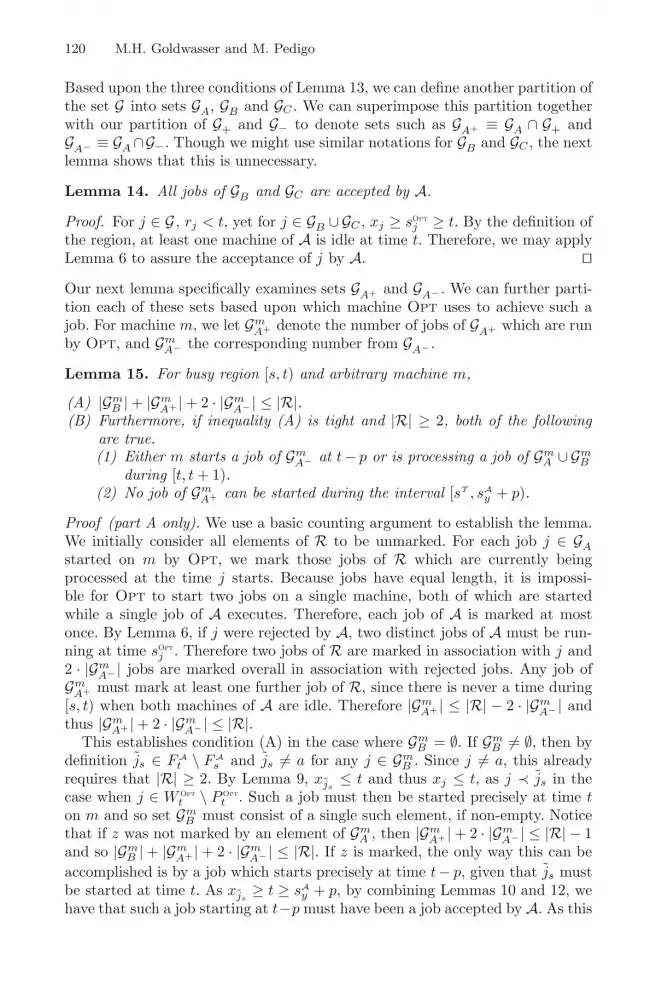
Based upon the three conditions of Lemma 13, we can define another partition ofthe set G into sets GA, GB and GC . We can superimpose this partition togetherwith our partition of G+ and G− to denote sets such as GA+ ≡ GA ∩ G+ andGA− ≡ GA ∩G−. Though we might use similar notations for GB and GC , the nextlemma shows that this is unnecessary.

Lemma 14. All jobs of GB and GC are accepted by A.

Proof. For j ∈ G , rj < t, yet for j ∈ GB ∪ GC , xj ≥ sOpt

j ≥ t. By the definition ofthe region, at least one machine of A is idle at time t. Therefore, we may applyLemma 6 to assure the acceptance of j by A. �

Our next lemma specifically examines sets GA+ and GA− . We can further parti-tion each of these sets based upon which machine Opt uses to achieve such ajob. For machine m, we let Gm

A+ denote the number of jobs of GA+ which are runby Opt, and Gm

A− the corresponding number from GA− .

Lemma 15. For busy region [s, t) and arbitrary machine m,

(A) |GmB | + |Gm

A+ | + 2 · |GmA− | ≤ |R|.

(B) Furthermore, if inequality (A) is tight and |R| ≥ 2, both of the followingare true.(1) Either m starts a job of Gm

A− at t − p or is processing a job of GmA ∪ Gm

B

during [t, t + 1).(2) No job of Gm

A+ can be started during the interval [sT , sAy + p).

Proof (part A only). We use a basic counting argument to establish the lemma.We initially consider all elements of R to be unmarked. For each job j ∈ GA

started on m by Opt, we mark those jobs of R which are currently beingprocessed at the time j starts. Because jobs have equal length, it is impossi-ble for Opt to start two jobs on a single machine, both of which are startedwhile a single job of A executes. Therefore, each job of A is marked at mostonce. By Lemma 6, if j were rejected by A, two distinct jobs of A must be run-ning at time sOpt

j . Therefore two jobs of R are marked in association with j and2 · |Gm

A− | jobs are marked overall in association with rejected jobs. Any job ofGm

A+ must mark at least one further job of R, since there is never a time during[s, t) when both machines of A are idle. Therefore |Gm

A+ | ≤ |R| − 2 · |GmA− | and

thus |GmA+ | + 2 · |Gm

A− | ≤ |R|.This establishes condition (A) in the case where Gm

B = ∅. If GmB �= ∅, then by

definition js ∈ F At \ F A

s and js �= a for any j ∈ GmB . Since j �= a, this already

requires that |R| ≥ 2. By Lemma 9, xjs≤ t and thus xj ≤ t, as j ≺ js in the

case when j ∈ W Opt

t \ P Opt

t . Such a job must then be started precisely at time ton m and so set Gm

B must consist of a single such element, if non-empty. Noticethat if z was not marked by an element of Gm

A , then |GmA+ | + 2 · |Gm

A− | ≤ |R| − 1and so |Gm

B | + |GmA+ | + 2 · |Gm

A− | ≤ |R|. If z is marked, the only way this can beaccomplished is by a job which starts precisely at time t − p, given that js mustbe started at time t. As xjs

≥ t ≥ sAy + p, by combining Lemmas 10 and 12, we

have that such a job starting at t−p must have been a job accepted by A. As this


accepted job marks both y and z, again we find that |GmA+ | + 2 · |Gm

A− | ≤ |R| − 1and so |Gm

B | + |GmA+ | + 2 · |Gm

A− | ≤ |R|. This establishes part (A) in general. �

Lemma 16. For u ∈ G+, us ∈ (F At ∪ P A

t ) \ (F As ∪ P A

s ).

Lemma 17. For distinct u, v ∈ G , us and vs are distinct.

Lemma 18. If as ∈ QOpt

t for region [s, t), then as ∈ W Opt

t and a �∈ P As .

Lemma 19. For busy region [s, t), assume that as ∈ QOpt

t and there exists someb ∈ P A

s ∪ W At . We may legally establish a match, Mt(b) = as.

Lemma 20. If ΦOpt

s ≤ ΦAs for busy region [s, t), then ΦOpt

t ≤ ΦAt .

Proof (sketch). For ease of exposition, we introduce notation ΦA[s,t) to denote

(ΦAt − ΦA

s ), and likewise ΦOpt

[s,t) = (ΦOpt

t − ΦOpt

s ). Our goal is to show that ΦOpt

[s,t) ≤ΦA

[s,t). In accordance with Lemmas 13 and 14, we rewrite ΦOpt

[s,t) as,

ΦOpt

[s,t) = 2 · |G| = 2 · |Gm1A+ ∪ Gm2

A+ ∪ Gm1A− ∪ Gm2

A− ∪ Gm1B ∪ Gm2

B ∪ GC |= (|Gm1

B | + |Gm1A+ | + 2 · |Gm1

A− |) + (|Gm2B | + |Gm2

A+ | + 2 · |Gm2A− |) + |GC |

+ |Gm1A+ ∪ Gm2

A+ ∪ Gm1B ∪ Gm2

B ∪ GC |= (|Gm1

B | + |Gm1A+ | + 2 · |Gm1

A− |) + (|Gm2B | + |Gm2

A+ | + 2 · |Gm2A− |) + |GC | + |G+|

By applying Lemma 15(A) to each of the two machines of Opt, we conclude thatΦOpt

[s,t) ≤ 2 · |R|+ |GC |+ |G+|. In contrast, we claim that ΦA[s,t) ≥ 2 · |R|+ δ + |G+|,

where δ is defined as

δ =

⎧⎨

⎩

1 if P As = ∅ and P A

t �= ∅−1 if P A

s �= ∅ and P At = ∅

0 otherwise

The δ term adjusts for the discontinuity inherent in our definition of ΦA, basedupon whether or not set P A is empty. With that aside, each job of R results ina relative contribution of at least 2, as such job is added to F A though perhapsremoved from P A. The only other way in which a job can be removed fromP A is if it becomes matched. We consider the creation of a new match in oneparticular case. If as ∈ QOpt

t and there exists some b ∈ P As ∪ W A

t , we createa match, Mt(b) = as, with the validity of such a match established as perLemma 19. In this special case there is indeed a relative loss of one unit due tojob b. However as as ∈ W Opt

t , we show that a �∈ P As . If it were, then a would

be unmatched at time s, thus as = a, yet since a ∈ QOpt

t it is not possible thata ∈ P A

s ⊆ W As = QA

s \ QOpt

t . Given that a �∈ P As , its presence in R results in a

profit of 3 rather than the minimally assumed profit of 2 and so this offsets theloss of 1 due to the matching of b.

Next, we consider the impact of set G+ on ΦA[s,t). By Lemma 16, for any u ∈ G+

there exists us ∈ (F At ∪P A

t )\ (F As ∪P A

s ) and by Lemma 17, those associated jobsare distinct. Each such job provides an additional point towards ΦA

[s,t) beyond


the presumed 2 · |R|, either providing 1 if in P At , or providing 3 rather than

2 if in F At . It is important to note that these |G+| additional points are also

distinct from the possible point associated with a in the preceding paragraph,as in that case neither a nor as can lie in G+. We have thus far established thatΦA

[s,t) ≥ 2 · |R| + δ + |G+|.For the remainder of the proof, we focus on the expression (δ−|GC |), recalling

that |GC | is either 0 or 1. In the case that (δ − |GC |) ≥ 0 the theorem follows, asΦOpt

[s,t) ≤ 2 · |R| + |GC | + |G+| ≤ 2 · |R| + δ + |G+| ≤ ΦA[s,t).

If (δ − |GC |) < 0 we undertake a detailed case analysis to counterbalancethis deficit either by showing a gap in our upper bound on ΦOpt

[s,t) due to a strictinequality when applying Lemma 15(A) to one or both of the two machines ofOpt, or by showing a gap in our lower bound on ΦA

[s,t). Details are omittedhere. �

Theorem 1. Algorithm A is 32 -competitive.

Proof. We show that ΦOpt

t ≤ ΦAt by induction. Initially, ΦOpt

0 = ΦA0 = 0. Neither

potential function changes during regions for which A remains completely idle,as per Lemma 5. The times during which A uses one or more machines can bepartitioned into regions [s, t), for which Lemma 20 applies, thereby extendingthe induction from time s to time t for each such region. We conclude thatΦOpt

∞ ≤ ΦA∞. Since the queues of both A and Opt are presumed to be empty at

t = ∞, P A∞ = P Opt∞ = ∅. Therefore, ΦOpt∞ ≤ ΦA∞ is equivalent to 2 · |F Opt∞ | ≤ 3 · |F A∞|,thus |Opt|

|A| ≤ 32 . �

Theorem 2. For m = 2, no non-preemptive, deterministic algorithm can bebetter than 3

2 -competitive.

Proof. Consider the release of a single job j = 〈0, 3p − 1〉. A deterministic al-gorithm must start j at some time 0 ≤ t ≤ 2p − 1, or else have unboundedcompetitiveness. Yet if two identical jobs with parameters 〈t + 1, t + 1 + p〉 aresubsequently released, one must be rejected. It is easy to verify that Opt canachieve all three jobs. �

Acknowledgments

We gratefully acknowledge the correspondence of Jirı Sgall.

References

1. P. Baptiste, P. Brucker, S. Knust, and V. G. Timkovsky. Ten notes on equal-processing-time scheduling. 4OR: Quarterly J. Belgian, French and Italian Oper-ations Research Societies, 2(2):111–127, July 2004.

2. S. K. Baruah, J. R. Haritsa, and N. Sharma. On-line scheduling to maximize taskcompletions. J. Combin. Math. and Combin. Computing, 39:65–78, 2001.


3. A. Borodin and R. El-Yaniv. Online Computation and Competitive Analysis.Cambridge University Press, New York, 1998.

4. M. Chrobak, W. Jawor, J. Sgall, and T. Tichy. Online scheduling of equal-lengthjobs: Randomization and restarts help. In J. Dıaz, J. Karhumaki, A. Lepisto,and D. Sannella, editors, Proc. 31st Int. Colloquium on Automata, Languages andProgramming (ICALP), volume 3142 of Lecture Notes in Computer Science, pages358–370, Turku, Finland, July 2004. Springer-Verlag.

5. J. Ding and G. Zhang. Online scheduling with hard deadlines on parallel ma-chines. In Proc. Second Int. Conference on Algorithmic Aspects in Informationand Management, Lecture Notes in Computer Science, Hong Kong, China, June2006. Springer-Verlag. To appear.

6. S. Goldman, J. Parwatikar, and S. Suri. On-line scheduling with hard deadlines.J. Algorithms, 34(2):370–389, Feb. 2000.

7. M. H. Goldwasser. Patience is a virtue: The effect of slack on competitiveness foradmission control. J. Scheduling, 6(2):183–211, Mar./Apr. 2003.

8. M. H. Goldwasser and B. Kerbikov. Admission control with immediate notification.J. Scheduling, 6(3):269–285, May/June 2003.

9. J. R. Jackson. Scheduling a production line to minimize maximum tardiness.Research Report 43, Management Science Research Project, University ofCalifornia, Los Angeles, Jan. 1955.

10. B. B. Simons. Multiprocessor scheduling of unit length jobs with arbitrary releasetimes and deadlines. SIAM J. Comput., 12:294–299, 1983.

11. B. B. Simons and M. K. Warmuth. A fast algorithm for multiprocessor schedulingof unit-length jobs. SIAM J. Comput., 18(4):690–710, 1989.

online, non-preemptive scheduling of equal-length jobs on two identical machines

Documents