on the use of panel research designs and random effects models to investigate static and dynamic...

ON THE USE OF PANEL RESEARCH DESIGNS AND RANDOM EFFECTS MODELS TO INVESTIGATE STATIC AND DYNAMIC THEORIES OF CRIMINAL OFFENDING

ROBERT BRAME SHAWN BUSHWAY RAYMOND PATERNOSTER*

University of Maryland National Consortium on Violence Research

There is a long-standing debate in criminology about the relative impact of static versus dynamic factors on criminal behavior. Research- ers interested in estimating the impact of dynamic factors like prior offending or association with delinquent peers on criminal offending must control for static factors like intelligence, family background, or self-control, which could plausibly be correlated with criminal offending and the dynamic factor itself Unfortunately, as a practical matter, it is not possible to observe all of these static factors. Statisticians and econometricians have shown that it is possible to identih the collective effect of static factors even though they cannot be observed. To achieve this objective, however, it is necessary to account for stable, unobserved individual characteristics through the use of ‘$xed-effect” or “random- effect ’’ estimation. Criminologists often use random-effect estimators in these situations. We describe some of the assumptions that are necessary to develop valid inferences when time-varying covariates are used. Then, we use simulation evidence and an empirical application to show that bias can result when they are violated.

THE ISSUE During the past two decades, criminologists have increasingly used lon-

gitudinal research designs to investigate how criminal offending develops and changes over the life span (see e.g., Blumstein et al., 1986; Elliott et al., 1985; Farrington, 1986; Greenberg, 1979; Loeber and LeBlanc, 1990; Saltzman et al., 1982; Sampson and Laub, 1993). Several empirical results have emerged from these efforts. For example, past and future criminal behavior are strongly associated with each other (Nagin and Farrington, 1992a, 1992b; Nagin and Paternoster, 1991; Sampson and Laub, 1993).

* The authors contributed equally to this article.

CRIMINOLOGY VOLUME 37 NUMBER 3 1999 599

600 BRAME ET AL.

Also, delinquent peer exposure is associated with involvement in criminal activity while marital and occupational attachments seem to be associated with desistance from criminal activity (Elliott et al., 1989: Laub et al., 1998; Sampson and Laub, 1993). No one disputes the fact that it is potentially useful to know that these correlations exist. Still, whether they are of any etiological importance is quite another matter. It is on this issue that criminologists leave the realm of consensus and enter a more ambiguous realm, where different criminologists have very different views.

In this article, we attempt to bring some of the sources of this dissensus out into the open. In so doing, we consider some of the available strategies for analyzing longitudinal records of criminal behavior. One such strategy, to which we devote the bulk of our discussion, involves the use of a collection of tools that we generically describe as mndom-effects models. Random-effects modeling strategies are receiving increased attention in contemporary criminology and hold the potential for significantly advanc- ing knowledge about the processes that generate criminal behavior at different points in the life span. In this article, we explore some of the properties of these models and the assumptions upon which their validity depends. We demonstrate the potential effect of particular violations of the assumptions on the validity of inferences about individual-level crime- generating processes. Finally, we illustrate the practical importance of these assumptions by reexamining some results previously reported in this journal.

THEORETICAL BACKGROUND

The strong positive association between past and future individual criminal activity is one of the most agreed, yet least well understood, facts about law-breaking behavior. Individuals who have offended in the past are most likely to offend in the future. There is little doubt or ambiguity about the validity of this claim. Still, it is not clear why this association exists. As Nagin and Paternoster (1991) observed nearly a decade ago, a number of very different explanations are all potentially capable of explaining the relationship between past and future criminal activity. For example, some theorists have argued that variation in criminal offending can be explained by variation in a time-stable predisposition to commit crimes (see e.g., Gottfredson and Hirschi, 1990: Wilson and Herrnstein, 1985). According to this point of view, differences between individuals in this propensity to offend are established early in life. Once established, these differences tend to endure. To these theorists, the relationship between past and future criminal activity is not causal. Rather, they contend, it can be explained entirely by enduring individual differences in the proclivity to offend (Nagin and Paternoster, 1991).

PANEL DESIGNS & RANDOM EFFECTS MODELS 601

Similarly, such theories also discount the etiological importance of many well-documented time-varying or dynamic correlates of criminal offending, such as school performance, delinquent peer exposure, and marital and occupational attachments. According to these stable-individual-difference theories, enduring dispositions to offend are synonymous with enduring dispositions to select delinquent peers for friends. They are synonymous with enduring dispositions to perform poorly in school and in the work- place. They are synonymous with the inability to enter into warm, mutu- ally satisfying marital relationships. The list could continue. In sum, stable-individual-difference theories maintain that the associations between well-documented crime correlates and criminal activity are spurious once relevant stable individual differences have solidified. For con- venience, we will refer to criminological theories that implicate only stable individual differences as static explanations.

A number of contemporary criminological theorists, however, have adopted a more dynamic position. Research that investigates the validity of these dynamic theories will, of necessity, be longitudinal in nature. According to dynamic theorists, the temporal development of criminal activity cannot be understood by appealing only to the continuing rever- beration of stable individual differences. And, it cannot be investigated by studying individuals at one point in time. Instead, dynamic theorists predict that life experiences (including criminal activity itself), changing social networks, and evolving perceptions will also explain why some people offend at particular time periods while others do not-even after the influence of stable individual differences has been taken into account (Horney et al., 1995; Laub et al., 1998; Loeber and LeBlanc, 1990; Nagin and Pater- noster, 1994; Sampson and Laub, 1993).

This latter point is especially important because there seems to be wide- spread agreement among criminologists that stable individual differences must be taken into account when estimating the effects of variables whose values are subject to change over time (see e.g., Nagin and Farrington, 1992a, 1992b). Numerous researchers have noted that a variety of problem behaviors, such as drug use, fighting, unemployment, marital instabil- ity, and crime, tend to cluster within the same individuals (see e.g., Donovan and Jessor, 1985; Laub et al., 1998 Nagin et al., 1995; Osgood et al., 1988; Robins 1966, 1978 Rowe and Flannery, 1994). While it may be the case that some problem behaviors causally increase the risk of involvement in other problem behaviors, an equally compelling rival hypothesis is that a collection of individual characteristics causally increases the risk of involvement in many different kinds of problem behavior. And, clearly, both processes may be operating at the same time.

Therefore, it is well settled that some attempt must be made to control for stable individual differences when estimating the effects of dynamic

BRAME ET AL.

factors on criminal behavior. In practice, however, not all of the relevant stable individual differences are observed. That they are not observed does not, of course, make them any less real, and therefore, it is also well settled that attempts must be made to control for stable but unobserved individual differences.

In sum, dynamic theorists would adopt the position that the resolution of the relative validity of static and dynamic explanations of criminal offending requires two things: (1) measures of individuals over time and (2) the ability to assess the impact of dynamic factors (e.g., job stability, marital satisfaction, and so on) on criminal offending net of stable individual differences. Sometimes, these individual differences are observed because there are available measures of things that capture criminal propensity (e.g., intelligence, parental criminality, impulsivity). More often, however, such measures are not available or are incomplete, and researchers must adopt some method for holding them constant. As we discuss in the next section, static theorists are generally of a different mind regarding the resolution of the debate.

METHODOLOGICAL IMPLICATIONS

The theoretical dispute about the etiological import of static and dynamic crime-producing factors has important methodological implications. In stark contrast to the position of dynamic theorists, the clear methodological implication of a static explanation is the adequacy of cross-sectional studies of crime and the corresponding irrelevance of longitudinal or panel studies. Gottfredson and Hirschi (1990:232), for example, argue that if differences in crime are due to stable individual differences in crime-proneness, longitudinal designs are simply unnecessary for drawing accurate inferences about processes that generate criminal behavior over the life span: “If there is continuity over the life course in criminal activity (or its absence), it is unnecessary to follow people over time.” Their argument can be summarized as follows: (1) issues of cause and effect are not easily resolved by nonexperimental longitudinal research designs; (2) current research strategies with panel data amount to little more than repeated cross-sectional analysis; and (3) the task of sorting out the validity of static and dynamic explanations of criminal behavior may best be resolved by experimental research.

In our view, Gottfredson and Hirschi make an important point. Other things being equal, experiments clearly provide a more credible basis for making causal inferences than panel designs. However, as Gottfiedson and Hirschi (1990:220) acknowledge, it is difficult to think of ways to create experiments to rigorously test key propositions of dynamic theories (or, to falsify static ones). How, for example, can one randomly assign


individuals to different kinds of marriages or different kinds of peer groups? This leaves an unhappy choice between nonexperimental cross- sectional designs and nonexperimental longitudinal designs. The question for criminologists, then, is whether one choice is more unhappy than the other. Gottfredson and Hirschi contend that the two designs are equally incapable of identifying causal effects, and cross-sectional designs should be preferred because of their lower cost. But, as they readily grant, this is a minority opinion in criminology (Blumstein et al., 1986; Farrington, 1986; Petersilia, 1980 Sampson and Laub, 1995).

A critical limitation of conventional cross-sectional analysis in distinguishing between static and dynamic explanations is that it does not allow estimation of the effects of dynamic factors while controlling for stable individual differences. In other words, cross-sectional designs cannot distinguish between the effects of variables whose values change over time and variables whose values do not. In fact, cross-sectional designs treat every explanatory variable as a static factor. But, when properly conducted, studies of panel data have the virtue that they can distinguish between the effects of variables whose values change over time and the effects of variables whose values are constant over time. If panel studies can help criminologists develop valid inferences about the effect of dynamic factors on criminal behavior while controlling for stable between- individual differences, the additional expense would seem to be justifiable.

If panel studies are potentially so helpful in assessing the merits of static and dynamic explanations of criminal behavior, why do Gottfredson and Hirschi seem to dismiss out of hand the utility of longitudinal designs? We think their position is more complex than a blanket rejection of panel analyses. Gottfredson and Hirschi’s view has always been that the current state of longitudinal analysis in criminology has failed to “deliver the goods” (where the “goods” are the ability to develop causal inferences from nonexperimental data). In our view, Gottfredson and Hirschi’s concerns about basing inferences on longitudinal analyses are more produc- tively seen as a challenge to the field than as anti-longitudinal dogma. In a commentary on the problem of developing valid causal inferences from longitudinal data, Hirschi (1987:2oO) observed that “it may not be possible to solve this problem by analysis of the data reflecting it, but it would be possible to do a better job.” In sum, Gottfredson and Hirschi seem to place the burden squarely on the shoulders of those who would do longitudinal analysis to demonstrate that the greater expense and labor inherent in the design are justified by the production of insights that cannot be obtained with cross-sectional analysis.

In this article, we respond to the challenge of Gottfredson and Hirschi

604 BRAME ET AL.

by examining the ability of one class of statistical models (as they are conventionally applied to longitudinal data) to help us develop valid inferences about the effects of dynamic factors on criminal behavior. Specifically, we focus on the so-called random-effects model. Random- effects modeling strategies provide criminological researchers with a very powerful set of tools for investigating the development of criminal offending over the life span. Based on our review of the criminological as well as the relevant statistical and econometric literature, we are convinced that the validity of inferences from random-effects models depends to some extent on assumptions that are not usually critically examined. Our own analysis convinces us that if these assumptions are not met, parameter estimates obtained from random-effects modeling efforts are likely to be biased. Moreover, the direction of the bias will tend to favor a dynamic rather than a static explanation of criminal behavior-a finding that sup- ports Gottfredson and Hirschi's skepticism about traditional panel-data analysis. But we also show that studies of longitudinal data sets can lead to approximately valid inferences about the influence of static and dynamic factors on criminal behavior under certain conditions.

The remainder of the article is organized as follows. First, we provide a brief conceptual introduction to random-effects modeling strategies. Next, we attempt to explain intuitively the technical assumptions underlymg these random-effects panel models. Then, using Monte Carlo simulation evidence, we show that parameter estimates will, in general, be biased when these assumptions are not met. Finally, we explain and implement some simple methods to reduce (but not entirely eliminate) those biases. We illustrate the application of these methods with more simulation evidence; we then revisit some analysis results that we previously published in this journal.

RANDOM-EFFECTS STATISTICAL MODELS1

Researchers are often interested in estimating the effects of variables whose values vary over time on criminal behavior. In criminology, classic examples of such variables include school performance, marital status, employment, delinquent peer exposure, and prior offending experience. The problem with obtaining valid inferences in these settings is that time- stable sources of criminality may be responsible for explaining at least some of the variation in all of these variables. Under these circumstances,

~

1. In this section, we try to provide some intuitive discussion about basic issues involved in random-effects model estimation. More formal treatments of these models can be found in most intermediate econometrics and statistics textbooks (see e.g., Greene, 1997; for a more specialized treatment see Hsiao, 1986).


at least some of the observed association between these time-varying variables and criminal behavior is spurious. If some of the confounding time- stable sources of criminality are not observed, it becomes more difficult to obtain valid inferences about the effects of time-varying variables.

Econometricians and statisticians have developed a number of methods that lead to valid inferences about the effects of observed time-varying variables in the presence of unobserved time-stable variables that are correlated with included time-varying variables. The most prominent of these methods are fixed-effects and random-effects panel models. Fixed-effect estimation undoubtedly provides the strongest control over the confounding influences of unobserved time-stable sources of criminality. The goal of fixed-effect estimation is to estimate a term for each individual in the data that takes all of the stable features of the process under study (i.e., criminal behavior) into account. This term is called a “fixed effect” and the data set can then be characterized by its distribution of fixed effects. After the fixed effects have been taken into account, the only variation that remains is variation due to individual change over time. Since the focus of this estimator is on explaining individual changes after the influence of stable individual differences has been removed, the estimated effects of variables in fixed-effects models are free of any confounding or bias that might be induced by these stable individual differences (see Allison, 1994, for a very helpful discussion of fixed-effect estimators).

While fixed-effect estimation clearly provides the strongest control over stable individual differences, it has some limitations in criminological work. First, it is more difficult to implement fixed-effect estimation when the outcome under study is qualitative rather than quantitative. Much criminological work focuses on variables such as whether an individual offends or how many times an individual offends within some finite time period. As King (1989) points out, it is not realistic to treat these sorts of discrete outcomes as realizations of a continuous data-generating process much less a continuous and normal data-generating process. It turns out, however, that traditional fixed-effect estimators are only consistent in qualitative outcome models when the number of time periods under study becomes large. In most contemporary criminological applications, the number of time periods under study is quite small (usually less than 15 to 20 periods). Thus, traditional fixed-effect estimation is not viable in this setting (see e.g., Hsiao, 1986:159; Maddala, 1987, 1993).

Some alternative fixed-effect estimators have been developed for qualitative outcomes. These methods involve the use of conditional likelihood functions (see e.g., Hausman et al., 1984 Maddala, 1987). In the case of binary or dichotomous outcomes, however, they are quite demanding in terms of the sample size because cases with certain kinds of outcome pat- terns drop out of the analysis entirely (Allison, 1994). In order to use

BRAME ET AL.

fixed-effect estimators to obtain consistent estimates about the effects of prior behavior on future behavior, it is necessary to make some strong assumptions about the absence of a linear time trend in the outcomes over the time period under study (Corcoran and Hill, 1984; Bushway et al., 1999).

Another common complaint about fixed-effects strategies is their inability to identify the effects of individual time-stable explanatory variables. Instead, the effects of all time-stable variables are captured by the “fixed effects” and are, therefore, treated as nuisances rather than as substantively interesting parameters. While this is not necessarily a bad thing (indeed, the strength of controlling for all time-stable confounding variables will often far outweigh the weakness of not estimating the effects of time-stable variables individually), it is something that should be considered when choosing an estimator.? Perhaps because of some of these reasons, fixed-effect estimators have not received much attention in longitudinal research in micro-level criminological studies. Instead, most contemporary criminological work has relied on random-effects estimation.

We define a random-effects estimator as a model that assumes that individual-specific effects are randomly drawn from some well-defined probability distribution (Hsiao, 1986:32-33). Random-effects models aiise in a variety of circumstances. For example, if one estimates a structural equation model (using LISREL or generalized least squares estimators) in which a dependent variable is observed at two or more time points for each individual and one allows for equal correlation between the residuals of the outcomes, then the structural equation model is a random-effects estimator (in the sense described here). One version of the hierarchical linear modeling (HLM) approach described by Bryk and Raudenbush (1992) can also be viewed as a random-effects model: specifically, when the HLM is implemented to allow for a random intercept (with no other random coefficients), it can be viewed as a conventional random-effects estimator.3

Random-effects estimators have also been implemented for qualitative

Researchers have often moved to other methods, primarily random-effects, when they wish to measure the impact of time-stable factors. As we show later, however, estimates of the coefficients of time-stable factors will always be biased in random-effects models because of confounding with unobserved heterogeneity. The choice, then, is not between measuring the impact of time-stable factors or not, but between not measuring their impact and measuring with bias.

As an anonymous reviewer noted. our results d o not necessarily apply to varia- tions of HLM and LISREL/GLS models that do not impose these constraints. It seems likely, however, that the kinds of problems we investigate here are not likely to be any easier to solve with the more complex models than they are with simpler models (such as those considered here).

2.

3.


outcomes within the HLM framework and in major software packages, like LIMDEP (Greene, 1995). with which random-effects probit models for binary outcomes and random-effects negative binomial models for event-count outcomes can be estimated. In standard generalized least squares, hierarchical linear models, and random-effects probit models, the available software typically operates under the assumption that the individual-specific effects are drawn from a normal probability distribution. The random-effects negative binomial model assumes that the random- effects are drawn from a beta probability distribution. Although other probability distributions for the random effects are possible (see e.g., Longford, 1995), in practice, the software to estimate models with other probability distributions is not yet widely available.

In recent years, Nagin and his colleagues have been engaged in a program of criminological research that allows for greater flexibility in the specification of the probability distribution from which the random effects are drawn (Land and Nagin, 1996; Land et al., 1996; Nagin and Land, 1993) for models with both qualitative and quantitative outcomes. In their framework, the shape of this distribution is not specified at all. It is only assumed to be discrete in form. Recent research using Wolfgang’s 1956 Philadelphia cohort has compared the results using the Nagin and Land semiparametric method to the standard random-effects method (Bushway et al., 1999). The results obtained from these two estimators are virtually identical, which indicates that for at least one prominent data set, assumptions about the probability distribution associated with the unobserved heterogeneity are either not violated or violated with little consequence. We conclude, therefore, that although concern about this assumption is legitimate, other aspects of the model are perhaps more problematic. In the next section, we describe two other key assumptions of the random- effects estimator that are often violated.

ASSUMPTIONS OF RANDOM-EFFECTS PANEL ANALYSIS

ZERO COVARIANCE BETWEEN THE ERROR TERM AND TIME-VARYING PREDICTORS

A potential issue with any given choice of model specification in the social sciences is the problem of omitted variable bias. Simply put, if some elements of the process that generates the outcome are not included in the model specification and those elements are correlated with the covariates that are included in the model, the parameter estimates associated with those covariates will be biased. We wish to emphasize that this is an important issue for cross-sectional and longitudinal analyses. Specifically, there are three different types of omitted variable bias in studies like the

608 BRAME ET AL.

kind we are discussing here.4 One type of bias occurs when time-stable omitted variables are correlated with time-stable included variables (type 1). For example, the coefficient estimate for the relationship between sex and offending will reflect both the effect of sex (a measured time-stable factor) and unmeasured levels of impulsivity (an unobserved time-stable factor correlated with sex). A second type of bias occurs when time-stable omitted variables are correlated with time-varying included variables (type 2). An example is when unobserved time-stable variables are correlated with a measured indicator of delinquent peers. A third and final type of omitted variable bias occurs when time-varying omitted variables are correlated with time-varying included variables (type 3). An example is when some or all of the effect of an included variable, like job status, is due to its correlation with an excluded variable also related to offending, such as a growing separation from unconventional peers.

In our view, type 1 bias is not unique to panel analysis, and is going to be very difficult to resolve.5 Type 2 bias is what we are concerned about here. Type 3 bias, which we think is more tractable than type 1, is an important problem but it is beyond the scope of this discussion.6 While we recognize that all three constitute potential pitfalls for those conducting

4. We thank a reviewer for emphasizing this issue. 5. This type of bias between observed and unobserved variables occurs in all

types of regression analysis, not just panel analysis. However, we believe that researchers using panel data and random-effects estimation often act as if the controls for unobserved heterogeneity eliminate the problem and yield an estimate for the included variable that gives its "true" value. This is not correct, since the random-effects model requires the assumption that there is no covariance between included and excluded variables. As noted by a reviewer, the coefficient on an included time-stable coefficient like sex will still provide an estimate of the "true" sex difference, but it concerns the unconditional relationship, not adjusted for any spurious or mediating factors. That can be useful information to know, but one must keep in mind that the results are subject to bias from the omitted variables, even in the random-effects framework.

A reviewer of our article mentioned two methods that may be helpful in resolving this problem. One method (originally used by Heckman) relaxes the constraint that all error terms are equally correlated with all other error terms. For example, such a general specification would allow the error terms at adjacent time periods to be more strongly correlated than the error terms at nonadjacent time periods. Another method would allow the time-trend effect to be a random rather than a fixed coefficient.

The first method allows for the possibility that there are variables whose effects endure for relatively short periods of time. The second method allows for the aggregate effect of omitted time-varying variables to vary across individuals. We think these are useful suggestions. We also think that estimators that approach this problem in different ways should be systematically compared in the future. Nevertheless, for the reasons discussed in this article, our main purpose is to deal with what we think is a more urgent issue: estimating the effects of time-varying variables when there are time-stable confounding variables.

6.


panel analyses with lie-course data, we acknowledge that the methods we have described deal only with the second type. Our interest in type 2 omitted variable bias is, of course, driven by our substantive interest in clearly delineating the influence of static and dynamic factors on criminal offending. This type of bias is particularly important because it involves a confounding of time-varying (dynamic) and time-stable (static) components. We believe that resolving this issue should constitute the first step for those interested in continuity and change in criminal offending. From our perspective, we thought that we should have a handle on the potential confounding of static and dynamic effects before we could comfortably move into a discussion of the relative impact of different dynamic factors. In a nutshell, our position is that at this current state of knowledge of the confounding issue, a concern with type 3 omitted variable bias is “putting the cart before the horse.”

To make the discussion of the type 2 bias more concrete, assume that an outcome variable, y,,, is a measure of criminal activity for each of i = I, 2, . . ., N individuals who are each observed at t = 1, 2, . . .. T time periods. Next, let q, be a measured time-stable variable, such as sex or race. We also let x,, be a measured time-varying variable, such as delinquent peer exposure, whether an individual is married, or job attachment. Now, we let T, be a term that captures all of the time-invariant factors that generate criminal behavior that are not measured (i.e., persistent unobserved sources of heterogeneity). While T, is an error term (because it captures the effects of variables that are not measured), it is not a random-error term. The term E,, is a random-error term that captures all of the omitted variables that affect criminal behavior at different time periods. A key feature of this error term is that it is uncorrelated with q,, x,,, and T,. TIe true crime-generating process in this case can be written as,

Yu = Pq, + 6x1, + 1, + E l f , (1) where p and 6 are parameters to be estimated.

Conventional fixed-effect estimators actually estimate the T, directly; the obvious cost of this procedure is that one is no longer able to estimate P. In the standard random-effects models commonly used in criminological research, each individual is assumed to draw a value of T, from a well- defined probability distribution. Random-effects estimators provide estimates of parameters associated with these probability distributions. For example, the GLSLISREL framework allows researchers to investigate the covariances of the error terms for the outcomes y,,. From these covariances, one can recover the parameters of the distribution governing the random effects. The validity of this procedure, however, depends on a critical assumption: T, must be uncorrelated with both q, and x,,. If the stable unmeasured sources of heterogeneity (i.e., T,) are correlated with q,,

610 BRAME ET AL.

any conventionally obtained estimate of p will be biased. Say, for example, that qi is an indicator of one’s sex and also assume that poor early parenting practices (e.g., lack of caring, or lax, harsh, and erratic disci- pline) are criminogenic and that they are unmeasured. In this case, p will not only indicate the effect of sex but it will also capture the effect of the part of sex that is correlated with poor parenting.

Similarly, if ii is correlated with xi*, the estimate of 6 will also be biased. For example, if delinquent peer exposure is the time-varying predictor, xi,, and if it is correlated with poor parenting, the estimate of 6 will capture both the true effect of delinquent peer exposure and the part of poor parenting that is correlated with delinquent peer exposure. In both cases, the biases are the logical outcome of a flawed model specification (classic omitted variable bias).

We refer to this as the zero-covariance problem and our question is whether it is possible to do anything about it. Unfortunately, as we demonstrate below, there is a two-part answer to this question. First, it is impossible to avoid bias in p when qi and ii are correlated with each other. Second, it is possible to reduce substantially the bias in 6 when xir and ii are correlated with each other. As Nagin and Paternoster (1991; see also Horney et al., 1995) have pointed out, such correlations are quite plausi- ble. Indeed, it is hard to envision realistic scenarios in which the zero- covariance problem could be ignored.

There are many theoretical reasons to expect a substantial positive association between unmeasured stable sources of criminality and measured covariates. A classic example, advanced by Hirschi (1969), is the conten- tion that the frequently observed positive correlation between delinquent behavior and delinquent peers is spurious rather than causal. His position is that there is something about delinquents that leads them to seek out like-minded others-the process by which “birds of a feather flock together.”

Although we have illustrated this point with delinquent peers as a time- varying variable, the existence of nonzero covariance could create problems for inference about many other time-varying variables as well. Consider, for example, indicators of marital or job satisfaction. One can easily imagine a time-stable component of mantaujob satisfaction that is also related to criminal offending, and of course, a time-stable component of offending that is related to marital/job satisfaction. Indeed, this is the very argument that Hirschi and Gottfredson (1995) make as to why reported “dynamic” effects are spurious. To assume that the covariance between unmeasured time-stable predictors of crime and measured time- varying predictors of crime is zero is unsatisfying precisely because this is the source of the theoretical controversy between static theorists and life- course dynamic theorists.


Further, as we show later, simply assuming that the covariance is zero when in fact it is not leads to estimates that overstate the impact of variables included in the model (both time-fixed and time-varying variables are affected). Notably, since time-varying variables can be biased, analyses that estimate important effects of time-varying covariates do not necessarily demonstrate that those effects are actually important. In our view, this is precisely the focus of Gottfredson and Hirschi’s critique of longitudinal research.

UNOBSERVED INITIAL CONDITIONS

Criminologists will often be interested in estimating a model that is slightly more complicated than Equation 1. A common alternative random-effects specification is to augment Equation 1 with a measure of prior criminal behavior, which we denote as yit.l. The model then takes the following form:

y;t = yyjI-i + P q i + axil + T; + ~ i r , (2) where y is an estimated regression coefficient. All of the other parameters have the same meaning as in Equation 1. The estimated effect of prior offending estimated by models of the form in Equation 2 is of substantial interest. As Nagin and Paternoster (1991) suggest, such an estimate measures the collective impact of unobserved time-varying variables whose effects are not confined to only one period of observation. In other words, the effect of any unobserved time-varying variable whose effects endure for more than one period will be incorporated into the estimate of the effect of prior offending. Intuitively, if all such time-varying variables were observed and all sources of unobserved stable heterogeneity had been taken into account, the estimated effect of prior offending on current offending would vanish (so long as the model was properly specified).

Note that for valid estimation of Equation 2 using random-effects methods, the zero-covariance assumption is still required because qi and xit are still in the model. The zero-covariance assumption is not needed for lagged y , however, because yir-] is handled differently from the other time- varying explanatory variables. But correlation between y,, and T~ is still a problem, albeit in a different way.

The model requires that the offending process be observed at the beginning, the so-called initial-conditions assumption. In the first period when any individuals begin offending ( t = l), y,, will be equal to zero for all individuals. If this is true, Y;, .~ will be uncorrelated with T~, the unobserved measure of individual heterogeneity. As a result, there will be no confounding between lagged y and unobserved heterogeneity in this first period. The error term will include the full amount of unobserved heterogeneity.

612 BFUME ET AL.

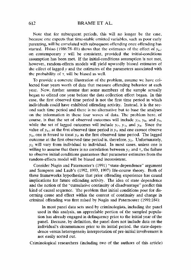
Note that for subsequent periods, this will no longer be the case, because one expects that time-stable omitted variables, such as poor early parenting, will be correlated with subsequent offending once offending has started. Hsiao (1986:78-81) shows that the estimates of the effect of Y,,.~ on contemporary y will be consistent, provided the initial-conditions assumption has been met. If the initial-conditions assumption is not met, however, random-effects models will yield upwardly biased estimates of the effect of lagged y and the estimates of the parameters associated with the probability of T, will be biased as well.

To provide a concrete illustration of the problem, assume we have col- lected four years worth of data that measure offending behavior at each year. Now, further assume that some members of the sample actually began to offend one year before the data collection effort began. In this case, the first observed time period is not the first time period in which individuals could have exhibited offending activity. Instead, it is the second such time period and there is no alternative but to base the analyses on the information in these four waves of data. The problem here, of course, is that the set of observed outcomes will include yI1, yi4, and y,, while the set of lagged outcomes will include Y , ~ , y,,, and yl4. Since the value of y,t-l at the first observed time period is yll and one cannot observe yIl, one is forced to treat y,, as the first observed time period. The lagged outcome at the first observed time period is, therefore, yI2. Unfortunately, yI2 will vary from individual to individual. In most cases, unless one is willing to assume that there is no correlation between y,, and T,, the failure to observe initial conditions guarantees that parameter estimates from the random-effects model will be biased and inconsistent.

Consider Nagin and Paternoster’s (1991) “state-dependence” argument and Sampson and Laub’s (1992, 1993, 1997) life-course theory. Both of these frameworks hypothesize that prior offending experience has causal implications for future offending activity. The idea of state dependence and the notion of the “cumulative continuity of disadvantage” predict this kind of causal sequence. The problem that initial conditions pose for dis- cerning cause and effect within the context of continuity and change in criminal offending was first raised by Nagin and Paternoster (1991:184):

In most panel data sets used by criminologists, including the panel used in this analysis, an appreciable portion of the sampled population has already engaged in delinquency prior to the initial year of the panel. Because, by definition, the panel does not include data on the individual’s circumstances prior to its initial period. the state-dependence versus heterogeneity interpretation of pre-initial involvement is not easily sorted out.

Criminological researchers (including two of the authors of this article)


have often not directly confronted the initial-conditions problem and have either ignored it or assumed that the initial conditions were exogenous. We examine below the extent to which this is a critical problem that cannot be assumed away when the model includes lagged measures of the dependent variable. We also implement a partial but useful solution to this problem.

In sum, it may appear that Gottfredson and Hirschi’s expressed skepticism about the capability of multivariate analysis of longitudinal data in distinguishing cause from effect is well-grounded. Random-effects panel analysis is fraught with potential pitfalls, and even with complex statistical treatment of the data it may be impossible to distinguish correlation from causality. Unless one is observing the onset of the causal process, or can make strong assumptions about its exogeneity, estimates of key parameters will be biased.

Recall, however, that even if the initial-conditions problem is resolved, not all of the bugs are out of the basement. We have previously discussed the problem that arises when there is a stable component of an explanatory variable that is correlated with the error term in the outcome variable. This problem will arise whenever stable individual crime-producing characteristics are correlated with variables such as delinquent peers, marital satisfaction, or job stability-in other words-many of the life-course events in which dynamic theorists are most interested. Unfortunately, we have thus far neither shown the magnitude of the problem (i.e., the extent to which parameter estimates are biased) nor suggested any reasonable solutions to these problems. In the next section we illustrate how severe the problems of initial conditions and zero covariance are for accurately estimating the structural parameters of random-effects panel models. Our platform for doing this is a series of simulations in which readers can see quite clearly the difference between the true and estimated parameter values when assumptions are violated. After documenting the magnitude of the bias when the assumptions of random-effects panel models are violated, we turn to a discussion of what we think are useful ways to address the initial-conditions and zero-covariance problems. We illustrate their application through additional simulations and a reanalysis of the data from a paper two of the current authors recently published, in which these problems were squarely at issue.

ASSESSING THE MAGNITUDE OF THE PROBLEM

The major points we wish to make can be illustrated through the use of a relatively simple set of simulations. In this section, our objective is to document the direction and magnitude of the estimation bias one can expect to encounter when the initial-conditions and zero-covariance assumptions are violated, under conditions similar to what is usually

614 BRAME ET AL.

encountered in the field. To achieve this objective. we simulated data for analysis with three kinds of statistical models commonly estimated by criminologists: (1) covariance structure (LISREL) (or, generalized least squares) models for continuous normally distributed outcomes: (2) probit models for binary outcomes: and (3) negative binomial models for event- count outcomes. Our simulations in each case involved samples of 500 individuals followed for five periods. The sample size and number of periods were chosen to approximate the size and nature of some of the more well-known panel data sets, like the National Youth Survey, the Rochester Youth Development Study, the Pittsburgh Youth Studv, the Denver Youth Study, Farrington’s Cambridge data, and the Gluecks’ data set recently analyzed by Sampson and Laub (1993).

The data were generated with five key components generally believed to exist in criminological data: (1) an observable, time-stable, individual- specific characteristic, like race or sex, written as ql; (2) an unobservable, time-stable, individual-specific characteristic, like intelligence or tempera- ment, written as 1,:’ (3) an observable, time-varying (dynamic) component, like marriage, employment, or delinquent peer exposure, written as x,,; (4) a time trend that allows for shifts in the overall rate of offending that correspond to the passage of time: and ( 5 ) a measure of offending that is causally dependent on observed and unobserved heterogeneity, the time trend, t , a time-varying, individual-specific component, and offending in the previous period, y,,.l. The q1 and T , were drawn from the standard unit bivariate normal distribution and allowed to be correlated at + 0.3. The time-varying covariate, xlt, was generated according to two protocols. Emst, we generated x,, by a first-order autoregressive process that depends on observed heterogeneity only. Then, we generated x,, by a first-order autoregressive process that depends on observed and unobserved heterogeneity. The correlation between individual heterogeneity and the dynamic component of the model is a fundamental issue in the current debate between dynamic and static models of criminal offending. For sim- plicity, the coefficients on all variables except the time-trend indicator, t, were set to 0.5. The time-trend indicator coefficient was set to 0.1.

The three outcomes were generated by using the so-called “acceptance- rejection method” (see e.g., Fishman 1996:171-172). Briefly, implementation of this method requires access to a uniform random number generator and a program in which probability density or mass functions can be easily written down. Implementation details can be found in Algorithm AR, described by Fishman (1996:172). For the LISREL/GLS simulations, each simulated realization of the dependent variable is a draw from the normal

This ensures that there will be significant correlation between residuals of dif- 7. ferent time periods for the same individual.


distribution. For the probit simulations, each simulated realization of the dependent variable is a draw from the Bernoulli distribution. For the event-count simulations, each simulated realization of the dependent variable is a draw from a beta mixture of negative binomial distributions.

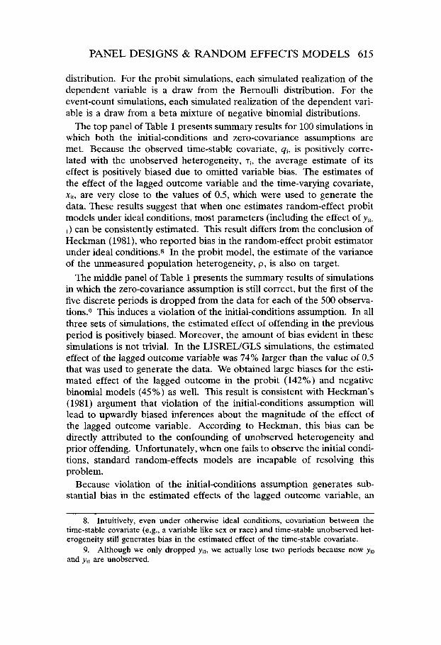
The top panel of Table 1 presents summaiy results for 100 simulations in which both the initial-conditions and zero-covariance assumptions are met. Because the observed time-stable covariate, qi, is positively correlated with the unobserved heterogeneity, T ~ , the average estimate of its effect is positively biased due to omitted variable bias. The estimates of the effect of the lagged outcome variable and the time-varying covariate, xit, are very close to the values of 0.5, which were used to generate the data. These results suggest that when one estimates random-effect probit models under ideal conditions, most parameters (including the effect of yi,. ,) can be consistently estimated. This result differs from the conclusion of Heckman (1981), who reported bias in the random-effect probit estimator under ideal conditions.8 In the probit model, the estimate of the variance of the unmeasured population heterogeneity, p, is also on target.

The middle panel of Table 1 presents the summary results of simulations in which the zero-covariance assumption is still correct, but the first of the five discrete periods is dropped from the data for each of the 500 observa- tions.9 This induces a violation of the initial-conditions assumption. In all three sets of simulations, the estimated effect of offending in the previous period is positively biased. Moreover, the amount of bias evident in these simulations is not trivial. In the LISREL/GLS simulations, the estimated effect of the lagged outcome variable was 74% larger than the value of 0.5 that was used to generate the data. We obtained large biases for the estimated effect of the lagged outcome in the probit (142%) and negative binomial models (45%) as well. This result is consistent with Heckman's (1981) argument that violation of the initial-conditions assumption will lead to upwardly biased inferences about the magnitude of the effect of the lagged outcome variable. According to Heckman, this bias can be directly attributed to the confounding of unobserved heterogeneity and prior offending. Unfortunately, when one fails to observe the initial conditions, standard random-effects models are incapable of resolving this problem.

Because violation of the initial-conditions assumption generates substantial bias in the estimated effects of the lagged outcome variable, an

8. Intuitively, even under otherwise ideal conditions, covariation between the time-stable covariate (e.g., a variable like sex or race) and time-stable unobserved heterogeneity still generates bias in the estimated effect of the time-stable covariate.

9. Although we only dropped yil, we actually lose two periods because now yio and yi, are unobserved.

Tabl

e 1.

Si

mul

atio

n R

esul

ts f

or L

ISR

EL

, Pro

bit,

and

Neg

ativ

e B

inom

ial

Mod

els

(1)

(2)

(3)

Initi

al C

ondi

tions

N

ot O

bser

ved

and

cov(

x,~J

> 0

Neg

ativ

e N

egat

ive

Neg

ativ

e L

ISR

EL

Pr

obit

Bin

omia

l L

ISR

EL

Pr

obit

Bin

omia

l L

ISR

EL

Pr

obit

Bin

omia

l Pa

ram

eter

T

rueV

alu

eE

u l?

u E

u E

u

E

u E

u

Ea

E

u E

u

Initi

al C

ondi

tions

Obs

erve

d In

itial

Con

ditio

ns N

ot O

bser

ved

--- ---------------

Con

stan

t Ti

me

Inde

x Ti

me

1 D

umm

y Ti

me

2 D

umm

y Ti

me

3 D

umm

y Ti

me

4 D

umm

y Ti

me 5

Dum

my

Tim

e-St

able

Cov

aria

te (

9)

Tim

e-V

aryi

ng C

ovar

iate

(x)

La

gged

Out

com

e P a B E

ndog

enou

s C

ovar

ianc

e $1

1

$22 4J 33

$44 c 55

-1.5

0.

I -1

.4

-1.3

-1

.2

-1.1

-1

.0

0.5

03

0.

5 0.

5 -

-

0.9

1.8

1.8

1.8

1.8

1.8

-1.5

01

.126

2.

669

.941

-1

.317

.I6

9 1.

682

.797

-1

.343

.20

6 ,6

60

.452

.lo0 ,0

30

.I01

.016

.0

60.0

41

.083

,0

25

,059

.051

,0

86

,026

-I

,40

3 ,0

66

-1 28

3 .0

67

-1.1

88 .

069

-.456

,07

0 -.S

60.0

65

- 1.

085 ,

069

-.280

.072

-.3

99.0

62

-.997

.08

2 -.

194

.065

-.3

18.

056

.803

.058

.7

90 .0

92

,795

,0

66

.19S

,046

,4

43 ,0

80

.736

,0

68

,163

,034

.3

14 ,0

59

,542

,0

66

.499

.025

.4

98 ,0

43 .SO3

,024

.4

20.0

34

.38 1

.053

SO

0 .0

30

,582

,029

,6

31 ,0

48

,638

,0

40

SO2

,020

SO

5 ,1

19

,493

.0

58

,870

,023

1.

210

,139

.7

2S

.I 13

,8

16 ,0

16

1.19

2 ,1

07

.884

.I23

.4

73 ,0

52

.060

.095

,0

02 .o

I I 7.

5.89

8 92

.722

31

.075

40.

293

19.5

06 8

.517

1.

117

,114

1.

354

.213

2.

461

.468

36

9 ,0

92

-.I01

.04

S -.

109.

034

1.16

9 ,0

74

1.83

8 .I2

0 1.

367.

084

1.82

0 .0

98

1.19

2 ,0

84

1.13

0 ,0

74

1.83

3 ,1

17

I. 12

6 ,0

76

1.13

8.07

8 1.

839 .

I24

1.83

6 .I1

4

NO

TE:

p in

dexe

s th

e co

rrel

atio

n be

twee

n th

e er

ror t

erm

s of

the

vario

us w

aves

for t

he p

robi

t mod

el.

The

a an

d p t

erm

s gov

ern

the

beta

dis

tribu

tion

from

whi

ch th

e ne

gativ

e bi

nom

ial r

ando

m e

ffec

ts a

re d

raw

n. T

he V

sym

bols

repr

esen

t the

var

ianc

es o

f th

e de

pend

ent

varia

ble

at e

ach

wav

e of

the

pa

nel,

whi

le th

e en

doge

nous

cov

aria

nce

capt

ures

the

cova

rianc

es b

etw

een

the

erro

r te

rms

of t

he v

ario

us w

aves

. T

hese

term

s ar

e as

soci

ated

with

the

LIS

RE

L/G

LS

spec

ifica

tion.

We

use

the

teim

E t

o de

note

the

expe

cted

val

ue o

f th

e pa

ram

eter

(av

erag

ed a

cros

s th

e se

t of

sim

ulat

ion

resu

lts),

and

the

term

u is

use

d to

den

ote

the

stan

dard

dev

iatio

n.


interesting question is whether this bias also contaminates other parameter estimates. In general, the answer to this question appears to be yes. In the GLSLISREL and probit frameworks, our estimates of the effects of q, and x,, were negatively biased. In the negative binomial framework, the estimated effect of q, is positively biased while the estimated effect of x,, is essentially on target. In the probit model, there also is evidence of negative bias in the estimated effect of unobserved population heterogeneity since the lagged outcome absorbs much of the variability attributed to static factors. The estimated coefficient of 0.060 for p underestimates the true value of S O by 88%.

The far right panel of Table 1 shows the consequences of violating both the initial-conditions and zero-covariance assumptions. In each of our three models, parameter estimates associated with the time-stable covariate q, and the lagged outcome variable continue to be biased. More- over, the estimates associated with x,, are now positively biased because x,, and T, are positively correlated. Finally, while the true value of unobserved heterogeneity in the probit model is SO, the mean estimated value of p is only .002 when both assumptions of the random-effects model are violated.

The bias also propagates to other parameter estimates when both assumptions are violated. In the GLS/LISREL framework, there is a 63% bias in the estimate of the lagged outcome. In the probit and event-count frameworks, the bias is 138% and 97%, respectively. The positive bias for the time-varying dynamic covariate x,, is 8% in the GLYLISREL model and approximately 13% in the probit and event-count frameworks. The negative bias for the variance component, p, in the probit model is 99.6%. The reader should notice that the positive bias in both x,, and ylt.l and the negative bias for the estimated importance of unmeasured time-stable crime-producing factors, p, in the probit model is in the direction that exaggerates the importance of dynamic factors and understates the importance of static factors.

The importance of this last point cannot be overemphasized. If this had been an actual analysis with unobserved initial conditions, the model specification in the last column of Table 1 would lead us to numerous incorrect conclusions. First, we would have concluded that there is no unobserved heterogeneity in the data, even though this is clearly not the case. The dynamic factor captures all of the variation that should be attributed to static factors. Second, we would have grossly overestimated the importance of the effect of the lagged outcome. Third, the biases associated with q, and xltr while smaller, are also substantively important. Taken as a whole. the estimates from these models bear little resemblance to the values that were actually used to generate the data. Next, we address the

618 BRAME ET AL.

question of whether it is possible to improve on the poor performance of the estimators in Table 1.

PROPOSED SOLUTIONS INITIAL CONDITIONS

Frequently, it simply is not possible to observe the initial state of some causal process. This results in a violation of the initial-conditions assumption. When one is working with continuous, normally distributed outcomes, there are many options available to deal with the initial-conditions problem. Among the possibilities are conventional fixed-effect estimators and alternative random-effects estimators that make different assumptions about the relationship between the unobserved heterogeneity, T~ and yio. These options are discussed in detail in Kessler and Greenberg (1981: Ch. 2 , 3 , and 7) and Hsiao (1986:Z-96). Our experience with these estimators suggests that they perform quite well in situations in which one can assume that the outcome variable is normally distributed. Moreover, these estimators are simple to implement with well-known software packages, such as SAS, Gauss, or S+. Unfortunately, as discussed above, most outcome variables studied by micro-level criminological researchers are either binary or event counts, and methods that take the discrete features of the data into account are necessary (Hsiao 1986:154-180). We focus the balance of our attention on remedies that can be used with qualitative outcomes.

When initial conditions are unobserved and cannot be assumed to be exogenous, Heckman (1981) provides the likelihood function that can be used to estimate the probability of offending in the first observed period. With current tools, this likelihood function is virtually intractable. Fortu- nately, he also provides a much simpler approximation from the available data. In the case at hand, the goal of the approximation is to estimate the probability of offending in the first period net of the individual’s underly- ing criminal propensity. In other words, if one cannot actually observe the initial conditions and cannot assume that it is exogenous, one can estimate the approximate state at the beginning of the series-that is, one can estimate the initial conditions from available data (Heckman 1981:188; Hsiao 1986:169-172). Since this solution approximates the state of initial conditions, we call it the Heckman approximation.

Implementation of the Heckman approximation is fairly straightfor- ward. Exogenous variables at the first wave are used to estimate the reduced-form marginal probability of offending at that wave. This probability is estimated from an auxiliary probit regression model, and the estimated probability of offending at the first wave of data from this model is used to “stand in” for the actual observed value of criminal activity.


Essentially, then, one takes the predictor variables from the first available wave, identifies exogenous variables to predict criminal offending, estimates a probit regression model for criminal offending for that wave, and then uses this estimated probability in subsequent panel analyses of the data in place of the observed value for the first wave.

In our example from above in which we did not observe the causal process until the second time period, assume that we were able to locate an exogenous variable qi that predicts participation in criminal activity. In the Heckman approximation, we would then take this exogenous variable and estimate the following probit equation for the probability of offending at the second wave:

p b 2 = 1) = WI + eqji, (3) where q and 0 are estimated probit coefficients and @[.I is the standard normal cumulative distribution function. Next, we enter this estimated probability of time 2 offending into the equation for time 3 offending. Thus, the probit equation for time 3 offending takes the following form:

yo* = aj + pqj + 6xiq + yPr(y2 = 1) + T; + E ; ~ , (4) where p(yi2 = 1) is obtained from Equation 3, a3 is the value of yi3* when all of the covariates are equal to zero, and

0 if yi7* I 0 1, ify$ > 0 . Yu =

To implement the Heckman approximation, it is appropriate to use variables that are available in the first observed time period. In practice, an auxiliary probit model can never include all of the characteristics that generate variation in offending propensity and, therefore, not all of the bias will be eliminated by this procedure. Still, the bias will be smaller with the Heckman approximation than if the initial-conditions problem is simply ignored.10

10. One reviewer suggested that the initial-conditions problem can be ameliorated by obtaining data sets in which the number of time periods is large. This was an intrigu- ing suggestion to us. In order to investigate it, we conducted a Monte Carlo simulation experiment in which we generated 17 periods of data in a form that we could estimate the random-effect probit model. In this simulation, the true effect of the lagged outcome was 0.3. We then dropped the first period entirely, and the second period outcome was used only to supply the lagged outcome for the third period. We then estimated the random-effect probit model using periods 3-7. The estimated effect of the lagged outcome was 0.8, evidencing substantial bias. We then estimated the probit model using periods 3-12. In this model, the estimated effect of the lagged outcome was 0.52, evidencing nonignorable but less substantial bias. Next, we estimated the probit model using periods 3-17. The estimated effect of the lagged outcome was 0.32, virtually on target. In the model in which the initial conditions were observed, the

BRAME ET AL.

ZERO COVARIANCE

Recall that the zero-covariance problem is essentially a specification error that is caused by omitted variable bias. That is, some of the variation in the predictor variables could be covarying with stable, unmeasured differences in the tendency to offend. To the extent that such covariation exists, one can expect parameter estimates to be biased and inconsistent. Unfortunately, for time-invariant covariates, such as sex and race, very little can be done to resolve this problem. For time-varying covariates, such as delinquent peers, job stability, or marital satisfaction, however, it may be possible to gain some improved accuracy in these situations.

A general solution to this problem involves the decomposition of xIt into two distinct components. The first component is the time-stable part of xlt, and the second component is the part of xlt that changes its values over time. The most promising approach available for accomplishing the objective of separating the between-individual variation in xIt from the within- individual variation in xlt in a random-effects framework is the procedure suggested by Bryk and Raudenbush (1992), employed in a recent paper by Homey et al. (1995). We continue to use delinquent peer exposure as our example of a time-varying independent variable.

The first, time-stable, component of the delinquent peer variable is each individual's level of delinquent peer exposure averaged across all of the waves of data. This captures between-individual variation in delinquent peer exposure. The second, time-vaiying, component of the delinquent peer variable is calculated separately for each time period within each individual person. For each person, we take the difference between the overall average delinquent peer exposure and the delinquent peer exposure at time t.

In order to separate the between-individual component of a time-varying covariate like delinquent peers from the within-individual component, the following steps should be followed: (1) for each individual, calculate the average level of delinquent peer exposure across all waves:

estimated effect of the lagged outcome was 0.28. On the basis of this evidence, we conclude that this reviewer's intuition that the initial-conditions problem could be ade- quately handled with more waves of data was correct. For researchers fortunate to have access to data sets with numerous time periods (bias was ignorable with about 15 time periods), then, there is another way to tackle the initial-conditions problem. How- ever, we must note that few publicly available data sets in criminology will allow researchers to appeal to this "big T" solution. Most panel data sets in criminology have a far more limited number of observation periods. In that instance, the solution we propose here is going to be the solution of choice. Although alternative data collection strategies promise "big T" data sets (like diary methods), these are still infrequent in our field.


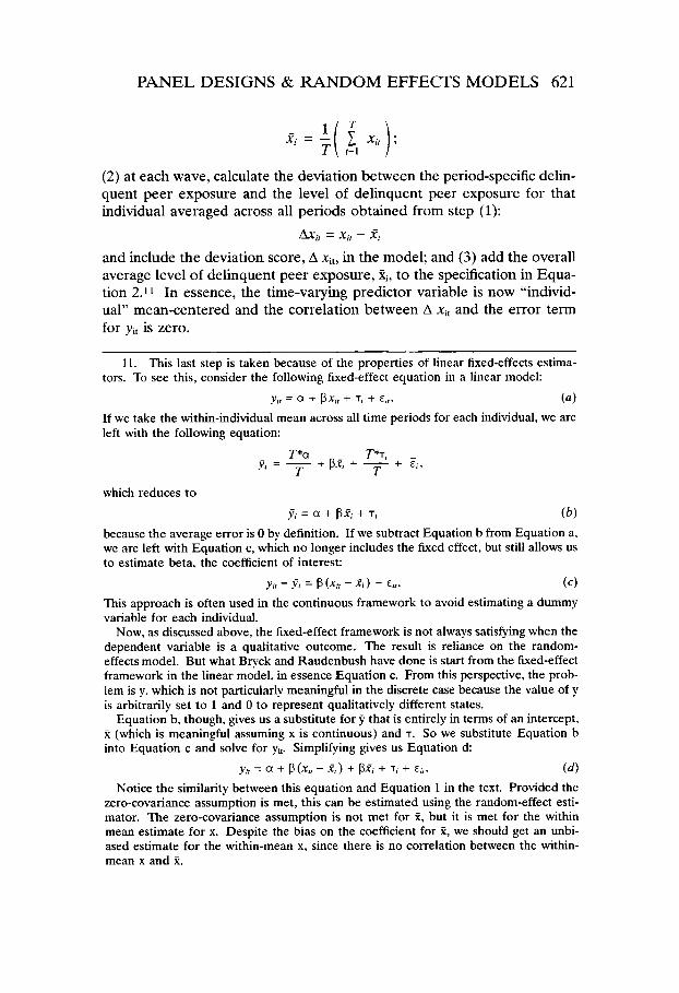
(2) at each wave, calculate the deviation between the period-specific delinquent peer exposure and the level of delinquent peer exposure for that individual averaged across all periods obtained from step (1):

&. - x . - 3.

and include the deviation score, A xit , in the model; and (3) add the overall average level of delinquent peer exposure, Ti, to the specification in Equa- tion 2.11 In essence, the time-varying predictor variable is now “individual” mean-centered and the correlation between A xit and the error term for yit is zero.

11 - D I

~

11. This last step is taken because of the properties of linear fixed-effects estimators. To see this, consider the following fixed-effect equation in a linear model:

y,, = a + Px,, + T, + E,,. ( a )

If we take the within-individual mean across all time periods for each individual, we are left with the following equation:

Fa = - T +p; x + - ma T + E,, Tea

which reduces t o

y, = a + pz, + 1, ( b ) because the average error is 0 by definition. If we subtract Equation b from Equation a, we are left with Equation c, which no longer includes the fixed effect, but still allows us to estimate beta, the coefficient of interest:

y,, - ?I = p (4, - d ) + El,. ( c ) This approach is often used in the continuous framework to avoid estimating a dummy variable for each individual.

Now, as discussed above, the fixed-effect framework is not always satisfying when the dependent variable is a qualitative outcome. The result is reliance on the random- effects model. But what Bryck and Raudenbush have done is start from the fixed-effect framework in the linear model, in essence Equation c. From this perspective, the problem is 7, which is not particularly meaningful in the discrete case because the value of y is arbitrarily set to 1 and 0 to represent qualitatively different states.

Equation b, though, gives us a substitute for 7 that is entirely in terms of an intercept, f (which is meaningful assuming x is continuous) and T. So we substitute Equation b into Equation c and solve for y,,. Simplifying gives us Equation d:

y , , = a + p ( ~ , , - - , ) + p ~ , + + , + ~ , , . (4 Notice the similarity between this equation and Equation 1 in the text. Provided the

zero-covariance assumption is met, this can be estimated using the random-effect estimator. The zero-covariance assumption is not met for j t , but it is met for the within mean estimate for x. Despite the bias on the coefficient for X, we should get an unbiased estimate for the within-mean x, since there is no correlation between the within- mean x and %.

622 BRAME ET AL.

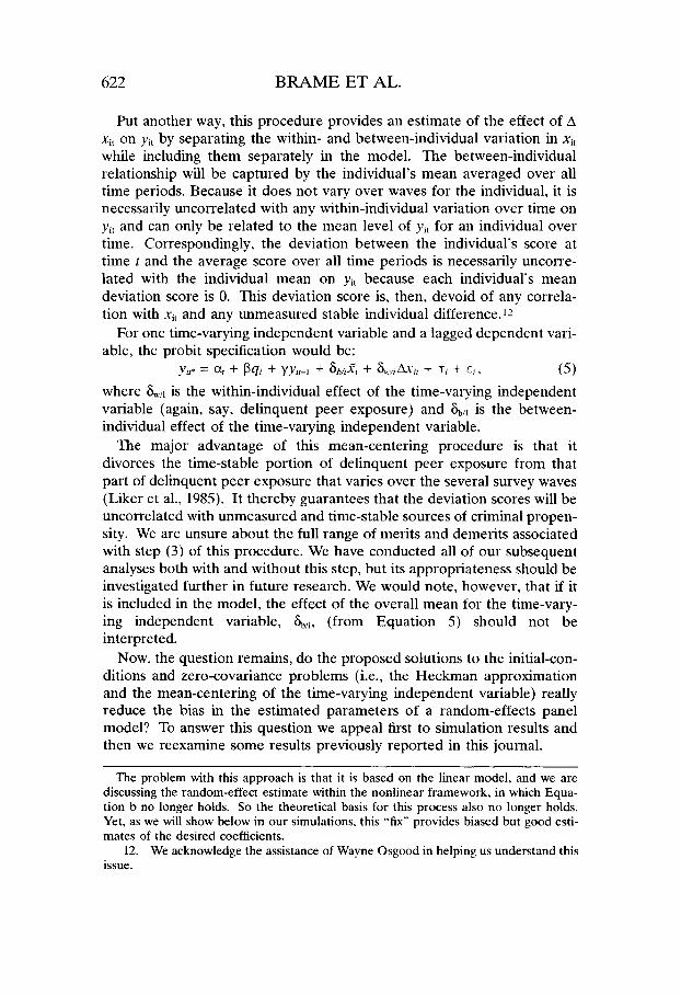
Put another way, this procedure provides an estimate of the effect of A x,, on y,, by separating the within- and between-individual variation in xIt while including them separately in the model. The between-individual relationship will be captured by the individual’s mean averaged over all time periods. Because it does not vary over waves for the individual, it is necessarily uncorrelated with any within-individual variation over time on y,, and can only be related to the mean level of ylt for an individual over time. Correspondingly, the deviation between the individual‘s score at time t and the average score over all time periods is necessarily uncorrelated with the individual mean on y,, because each individual’s mean deviation score is 0. This deviation score is, then, devoid of any correlation with x,, and any unmeasured stable individual difference.’?

For one time-varying independent variable and a lagged dependent variable, the probit specification would be:

where &,I is the within-individual effect of the time-varying independent variable (again, say, delinquent peer exposure) and &,, is the between- individual effect of the time-varying independent variable.

The major advantage of this mean-centering procedure is that it divorces the time-stable portion of delinquent peer exposure from that part of delinquent peer exposure that varies over the several survey waves (Liker et al., 1985). It thereby guarantees that the deviation scores will be uncorrelated with unmeasured and time-stable sources of criminal propensity. We are unsure about the full range of merits and demerits associated with step (3) of this procedure. We have conducted all of our subsequent analyses both with and without this step, but its appropriateness should be investigated further in future research. We would note, however, that if it is included in the model, the effect of the overall mean for the time-varying independent variable, &,,, (from Equation 5 ) should not be interpreted.

Now, the question remains, do the proposed solutions to the initial-conditions and zero-covariance problems (i.e., the Heckman approximation and the mean-centering of the time-varying independent variable) really reduce the bias in the estimated parameters of a random-effects panel model? To answer this question we appeal first to simulation results and then we reexamine some results previously reported in this journal.

yIr* = a, + Pqi + yyir-1 + bd, + + 1, + E,, (5 )

The problem with this approach is that it is based on the linear model, and we are discussing the random-effect estimate within the nonlinear framework, in which Equa- tion b no longer holds. So the theoretical basis for this process also no longer holds. Yet, as we will show below in our simulations, this “fix” provides biased but good estimates of the desired coefficients.

12. We acknowledge the assistance of Wayne Osgood in helping us understand this issue.


SIMULATION RESULTS

In this section, we use simulations to investigate the performance of the suggested remedies to the estimation problems that arise when the initial- conditions and zero-covariance assumptions are violated. Our reported results are restricted to the probit model. We note, however, that we obtained similar results with the negative binomial estimator for event- count outcomes.

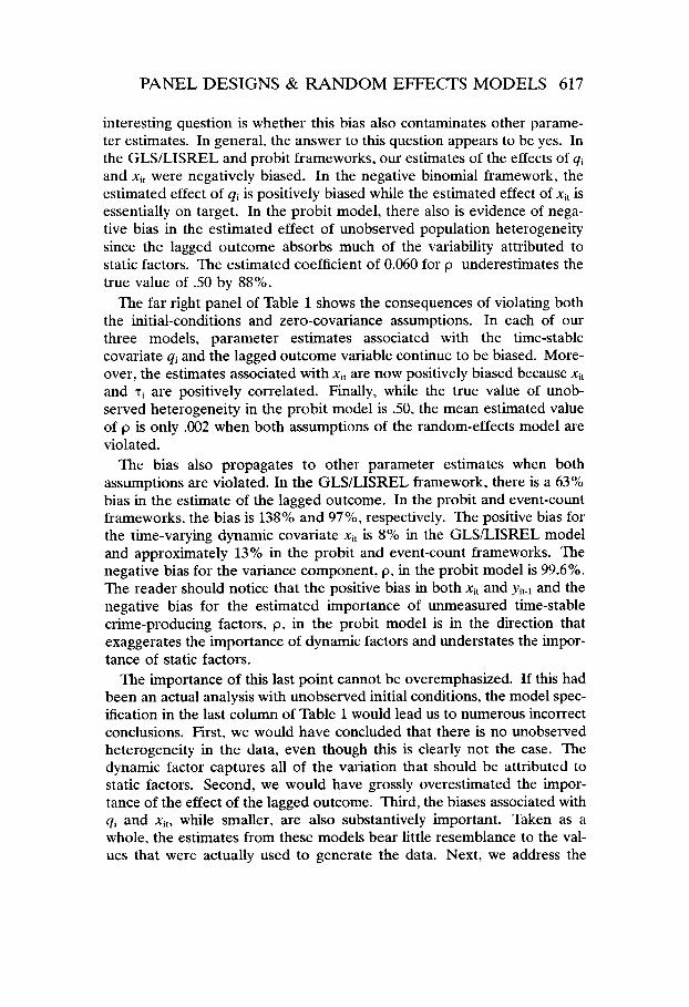
Table 2 presents three sets of probit simulation results. In the first panel of Table 2, we apply the Heckman approximation to the case in which initial conditions are not observed and the correlation between the time- varying independent variable, xil, and stable unobserved heterogeneity T~ is zero. The average parameter estimates for this simulation are very close to those for the ideal case (panel 1 of Table 1). The single exception to this general pattern is the negatively biased estimate of the effect of yil.l. Still, the bias in this estimate is dramatically smaller (14%) than the bias that results from simply ignoring the initial conditions problem (142%).

In addition, inferences based on this estimate will tend to be conservative since they understate the dynamic effect of the lagged outcome variable. It is also worth noting that the standard error of the effect of the lagged outcome variable is twice as large as what is observed with the naive estimator. In sum, while the Heckman approximation yields an improved average estimate of the effect of the lagged outcome, this improvement comes at the cost of increased sampling variability of that estimate.

In the second panel of Table 2, we turn to the case in which initial conditions are violated and there is a positive correlation between the time- varying covariate and unobserved time-stable individual heterogeneity. The probit simulations in this panel incorporate the Heckman approximation for initial conditions and the division of the time-varying covariate into between- and within-subject components. As expected, the introduction of correlation between the time-stable unobserved heterogeneity and the time-varying covariate leads to some deterioration in the accuracy of the parameter estimates. The simulation results indicate that the variance component that measures the importance of unmeasured time-stable crime-generating processes, p, the effect of the lagged outcome, yil-l, and the effect of the time-invariant predictor variable, qi, are all underesti- mated, while the effect of the between-individual component of the time- varying covariate is dramatically overestimated. Apparently, the between- individual component of the time-varying covariate captures a great deal of the static information in the data. The average estimate of the within- individual component, however, is very close to the true parameter value. As Horney et al. (1995) have indicated, if one’s substantive interest is in

Tabl

e 2.

Pr

obit

Sim

ulat

ions

with

Cor

rect

ions

for

Ini

tial

Con

ditio

ns a

nd Z

ero-

Cov

aria

nce

Prob

lem

s

Para

met

er

True

Val

ue

Con

stan

t Ti

me

Inde

x Ti

me-

Stab

le C

ovar

iate

(9)

Ti

me-

Vai

ying

Cov

aria

te (.

Y )

Ave

rage

Lev

el o

f .r

Perio

d-Sp

ecifi

c D

evia

tion

of .Y

Lagg

ed O

utco

me

P

-1.5

0.

1 0.

5 0.

5 0.

5 0.

5 0.

5 0.

5

Cor

rect

ion

Usi

ng H

eckm

an‘s

In

stru

men

tal

Var

iabl

e M

etho

d C

oV(X

,T,)

=

0

~ ~

E

U

-1.5

18

,250

.I

01

.057

34

0 ,1

54

.517

,0

72

.428

,2

55

.5 16

,0

98

(2)

Cor

rect

ion

Usi

ng H

eckm

an’s

In

stru

men

tal V

aria

ble

Met

hod

with

CO

V(X

.T,) > 0

Sp

ecifi

catio

n In

clud

es A

vera

ge

Leve

ls a

nd P

erio

d-Sp

ecifi

c D

evia

tions

of

x

E a

-1.5

42

,030

,1

05

,067

.3

45

.I 19

1.46

7 ,2

25

.525

,0

69

.347

.2

57

,367

.1

15

(3)

Cor

rect

ion

Usi

ng H

eckm

an’s

In

stru

men

tal V

aria

ble

Met

hod

with

CO

V(X

,T,)

>

0;

Spec

ifica

tion

Incl

udes

Per

iod-

Sp

ecifi

c D

evia

tions

of

.r

E

a

z -1

.486

,2

74

m

m

c1

? r

,093

,0

64

1.12

6 ,1

95

.555

,0

77

,464

,2

38

,644

,0

79

NO

TE:

p in

dexe

s th

e co

rrel

atio

n be

twee

n th

e er

ror

teiin

s of

the

var

ious

wav

es f

or t

he p

robi

t m

odel

. We

use

the

term

E t

o de

note

the

exp

ecte

d va

lue

of t

he p

aram

eter

(av

erag

ed a

cros

s th

e se

t of

sim

ulat

ion

resu

lts).

and

the

term

a is

use

d to

den

ote

the

stan

dard

dev

iatio

n.


the effects of time-varying covariates, this method appears to perform quite well.

Sometimes, of course, investigators wish to interpret the effect of the lagged outcome variable yi,-l as well as the effects of time-varying covariates. The method in the second panel of Table 2 does not perform well in this context. The third panel of Table 2 presents results of the simulation in which the between-individual component of the time-varying covariate was omitted from the model. These simulation results show that this omission leads to an improved estimate of the effect of the lagged outcome at the cost of a small increase in the bias of the estimated within- individual effect of the time-varying covariate. The results also indicate that the effect of the time-stable covariate, qi, is once again positively biased.

In sum, these simulations point to the conclusion that the covariance problem can be largely overcome. However, there is no complete remedy for the initial-conditions problem especially when the covariance problem also exists. Nevertheless, Heckman’s approximation produces much more accurate estimates of the effect of the lagged outcome variable provided appropriate predictor variables for estimating the probability of offending at the first wave are available.

REANALYSIS OF PREVIOUS WORK The problem of initial conditions and zero covariance arose in a panel

analysis reported by two of the current authors in a recent article in this journal (Paternoster and Brame, 1997).13 There were two substantive issues in that article: (1) Drawing on a theoretical debate between Hirschi and Gottfredson (1995) and Sampson and Laub (1995; see also Sampson and Laub 1993:197-200), we asked whether time-varying independent variables indexing prior offending activity and delinquent peer exposure were associated with participation in and frequency of criminal activity net of controls for observed and unobserved heterogeneity. (2) Drawing on the debate between general and typological theorists (Gottfredson and Hirschi, 1990: Moffitt, 1993; Patterson and Yoerger, 1993), we asked whether the effects of prior offending activity and delinquent peer exposure differed between high and low antisocial propensity groups.14

The data to examine these issues were obtained from the first five waves of the National Youth Survey (NYS). We selected only the two youngest

13. Because of space limitations, we present only a brief overview of our earlier study. Interested readers can consult the original article for greater detail.

14. The original study included both a behavior- and an attitude-based measure of antisocial propensity, and the categorization into high or low antisocial propensity groups was based on the use of different cutoff points.

626 BRAME ET AL.

age cohorts, those youth who were 11 or 12 years old at the first wave (N =509).15 After deleting cases that did not have sufficient data for the pro- cedures used in the analysis, the sample comprised 471 individuals. A subsample of 390 cases had complete data at all four remaining waves of data collection. We conducted all of the analyses reported in that article with the entire sample of 471 cases and with the subsample of 390 cases that had complete information.16

In favor of the position of dynamic theorists, the original findings suggested that the effects of delinquent peer exposure and prior offending activity exerted strong effects on criminal activity after controls for observed and unobserved individual differences had been taken into account. With respect to the debate on general and typological theories, we concluded that there was no evidence of important between-group variation in these effects.

In sum, our original analysis found strong support for general theories that anticipate important effects for time-varying variables. The parameter estimates in our original analysis were obtained from random-effects estimators (probit and negative binomial). For purposes of comparison, Table 3 restates the results of our original Table 4, and Table 4 restates the results of our earlier Table 6. In the following section, we revisit our previous results after employing the Heckman approximation for initial conditions and mean-centering the time-varying independent variable (delinquent peer exposure). In so doing, we attempt to provide better solutions to the problem of initial conditions and zero covariance than we employed in the original study.

As discussed earlier, when initial conditions are not observed, Heckman’s approximation can be used to estimate the probability of offending at the first wave. This probability is estimated from an auxiliary probit regression model. We identified six variables in the data that we thought were clearly exogenous: (1) respondent‘s sex; (2) respondent’s race; (3) whether the family receives public assistance; (4) whether the father was unemployed; ( 5 ) the age of the respondent’s youngest parent: and (6) the educational level of the respondent’s most well-educated parent. The specification of this equation was

P b l l = 1) = wl + % , I * (6)

15. Even after selecting on these two yougest age groups, we cannot plausibly claim that we have observed the initial conditions. Approximately 18% of these youth committed at least one offense during the first wave of data collection.

16. The analyses reported in our 1997 study were based on the sample of 471 cases. When cases with any missing data were excluded, however, all of the analyses in that study produced virtually identical results. In the current reanalysis, some of the results depend more heavily on cases with missing data.

Tabl

e 3.

B

asel

ine

Prob

it an

d N

egat

ive

Bin

omia

l M

odel

s U

nder

Orig

inal

Spe

cific

atio

n

Prob

it Pa

rtici

patio

n M

odel

s N

egat

ive

Bin

omia

l Fr

eque

ncy

Mod

els

Atti

tude

Pro

pens

ity

Beh

avio

r Pr

open

sity

A

ttitu

de P

rope

nsity

B

ehav

ior

Prop

ensi

ty

Mea

sure

M

easu

re

Mea

sure

M

easu

re

Var

iabl

e E

stim

ate

z R

atio

E

stim

ate

z R

atio

Es

timat

e z

Rat

io

Est

imat

e z

Rat

io

Con

stan

t -2

.900

14

.60

-2.8

76

14.7

8 -4

.398

18

.10

-4.4

84

18.4

4 Se

x =

Mal

e ,3

89

3.86

.3

79

3.86

.4

58

3.24

.4

61

3.21

R

ace

= N

onw

hite

.0

16

0.15

.0

23

0.21

.2

30

1.54

.2

29

1.44

Ti

me

Inde

x -.I

18

2.46

-.1

18

2.47

-.1

20

1.86

-.1

12

1.71

A

ny M

issi

ng W

aves

.2

38

1.66

.2

36

1.65

,0

30

0.20

.0

42

0.27

D

elin

quen

t Pee

r Ex

posu

re

.939

9.

92

.934

9.

86

1.13

2 13

.15

1.14

2 13

.33

Prio

r-W

ave

Del

inqu

ency

,8

37

6.84

36

2 7.

1 1

,959

6.

03

,984

6.

28

Hig

h-Pr

open

sity

Ind

icat

or

.406

2.

69

.332

2.

22

.445

2.

59

SO5

3.12

P

(dT

4d

T+

$")

) .0

80

0.61

.068

0.51

a

1.82

9 3.

95

1.92

8 3.

65

B 3.

538

2.19

3.

977

2.08

Lo

g Li

kelih

ood

-531

.99

-533

.30

- 109

3.88

-1

093.

03

NO

TE

: p

inde

xes

the

corr

elat

ion

betw

een

the

erro

r tei

ms o

f th

e va

rious

wav

es fo

r the

pro

bit m

odel

. T

he a

and

p te

ims g

over

n th

e be

ta d

istri

butio

n fr

om w

hich

the

neg

ativ

e bi

nom

ial

rand

om e

ffec

ts a

re d

raw

n.

Tab

le 4

. Pr

obit

and

Neg

ativ

e B

inom

ial

Mod

els

with

Int

erac

tion

Ter

ms

Und

er O

rigi

nal

Spec

ific

atio

n

Var

iabl

e

Con

stan

t Se

x =

Mal

e R

ace

= N

onw

hite

Ti

me

Inde

x A

ny M

issi

ng W

aves

D

elin

quen

t Pe

er E

xpos

ure

Prio

r-W

ave

Del

inqu

ency

H

igh-

Prop

ensi

ty I

ndic

ator

In

tera

ctio

n Te

rms

Prop

ensi

ty x

Del

. Pee

r Ex

p.

Prop

ensi

ty x

Prio

r D

elin

quen

cy

p (~

7/(

o’T

+a

?v))

a P Lo

g Li

kelih

ood

Prob

it Pa

rtici

patio

n M

odel

s

Atti

tude

Pro

pens

ity

Beh

avio

r Pr

open

sity

M

easu

re

Mea

sure

Est

imat

e z

Rat

io

Estim

ate

z R

atio

-2.8

75

,389

.0

17

-.I

18

,232

.9

22

,878

,3

55

14.1

1 3.

85

0.16

2.

48

1.61

9.

17

6.67

0.

85

-2.8

09

14.2

9 ,3

91

3.96

,0

23

0.2 I

-.1

16

2.41

,2

08

1.46

.8

96

9.13

A

31

6.45

-.3

87

0.66

,069

0.

33

,329

1.

20

-.I93

0.

64

,244

0.

86

,076

0.

56

.063

0.

47

-531

.70

-531

.92

Neg

ativ

e B

inom

ial

Freq

uenc

y M

odel

s

Atti

tude

Pro

pens

ity

Beh

avio

r Pr

open

sity

M

easu

re

Mea

sure

Estim

ate

z R

atio

E

stim

ate

L R

atio

-4.4

19

16.7

7 .4

63

3.22

.2

33

154

-. 12

3 I .8

5 ,0

12

0.07

1.

127

12.1

2 1.

070

6.29

,8

42

1.68

-4.4

40

17.9

4 .4

59

3.19

23

0 1.

43

-.115

1.

69

,039

0.

26

1.11

6 12

.29

1.00

4 6.

01

,217

0.

39

-.013

0.

06

,139

0.

64

-356

1.

42

-.035

0.

09

1.80

6 4.

00

1.95

8 3.

58

3.42

3 2.

20

4.10

9 2.

0s

-109

2.43

-1

092.

84

NO

TE:

p in

dexe

s th

e co

rrel

atio

n be

twee

n th

e er

ror t

eim

s of

the

vario

us w

aves

for t

he p

robi

t mod

el.

The

a an

d p t

erm

s go

vern

the

beta

dis

tribu

tion

from

whi

ch th

e ne

gativ

e bi

nom

ial

rand

om e

ffec

ts a

re d

raw

n.


where 8 is a vector of six probit regression coefficients conformable for multiplication with the vector of six exogenous variables: q1 = respondent's sex, q2 = respondent's race, q3 = whether the family receives public assistance, q4 = whether the father was unemployed, qs = the age of the respondent's youngest parent, and qb = the educational level of the respondent's most well-educated parent. In each case, it seems unlikely that variation in any of these variables could be caused by individual levels of criminal propensity or criminality.17

To deal with the problem of zero covariance between the time-varying independent variable and T ~ , we then mean-centered the measure of delinquent peer exposure at each wave. In our estimated equations, then, we included the estimated probability of offending at the first wave from Heckman's approximation and the mean-centered delinquent peer exposure variable. The results of our reanalysis are reported in Tables 5 and 6.

In Table 5, we present the parameter estimates of random-effects probit and negative binomial regression models with the full sample of N = 471 cases, and in Table 6 we present the regression models with the sample that had complete data at all four waves of data collection (N = 390). These two tables are comparable to Table 3 since they all impose the constraint that prior offending activity and delinquent peer exposure exert similar effects between the high and low antisocial propensity groups.

The results in Tables 5 and 6 suggest that the effect of prior offending activity is substantially attenuated from what was originally reported. We previously reported that the probit coefficient for prior offending was y = .837 (z value = 6.84) while holding an attitude-based measure of antisocial propensity constant and y = 362 (z value = 7.11) with a behavior-based measure of antisocial propensity held constant (see Table 3). In the cor- rected reanalysis with complete data (Table 5), these coefficients are reduced to .323 and .363, respectively, and are no longer statistically significant at conventional levels. When cases with missing data are included (Table 6), the attenuation is slightly less, with probit coefficients of .445 and .475 for the attitude and behavior measures of self-control, respectively. Both of these latter coefficients are significant at a .05 level, but

17. We would like to emphasize that the Heckman approximation is, in fact, an approximation. By definition, then. it is not a consistent estimator. Because it is not a consistent estimator, the literature provides no clear guidance on exactly how the first wave offending probability should be estimated. We tried several alternative schemes: (1) the method described above; (2) a method in which we included only the covariates in the substantive model (i.e., race, sex, delinquent peer exposure, and an indicator variable for high criminal propensity based on observed individual characteristics); and (3) a method in which we dropped the delinquent peer exposure measure but retained all of the other variables from (2). Of the three methods we compared, the one presented in the text of this paper produced the results at a greatest variance with those presented in our original analysis.

Q\ w

0

Tabl

e 5.

B

asel

ine

Prob

it an

d N

egat

ive

Bin

omia

l Mod

els

Usi

ng H

eckm

an's

App

roxi

mat

ion

Var

iabl

e

Con

stan

t Se

x =

Mal

e R

ace

= N

onw

hite

Ti

me

Inde

x M

ean

Del

inqu

ent

Peer

Exp

osur

e A

Del

inqu

ent

Peer

Exp

osur

e Pr

ior-

Wav

e D

elin

quen

cy

Hig

h-Pr

open

sity

Ind

icat

or

p (&

,4dT

+d")

) a P Lo

g Li

kelih

ood

Prob

it Pa

rtici

patio

n M

odel

s N

egat

ive

Bin

omia

l Fr

eque

ncy

Mod

els

Atti

tude

Pro

pens

ity

Mea

sure

B

ehav

ior

Prop

ensi

ty

Mea

sure

A

ttitu

de P

rope

nsity

M

easu

re

~~

Beh

avio

r Pr

open

sity

M

easu

re

Estim

ate

z R

atio

-3.6

50

9.74

.5

22

3.56

-.0

16

0.11

-.I

20

2.1

1 1.

34 1

7.46

,7

76

4.41

.3

23

1.33

,5

72

2.81

,2

69

1.83

-467

.33

Est

imat

e z

Rat

io

-3.6

33

10.1

1 .5

19

3.73

.oo

1 0.

0 1

-.120

2.

11

1.34

1 7.

69

.753

4.

28

.363

1.

56

.435

2.

17

,259

1 .s

o

-469

.25

Est

imat

e z

Rat

io

-4.8

53

,806

,1

06

1.71

4 1.

243

A02

.2

65

-.162

1.94

0 1.

882

-865

.70

12.7

1 4.

84

0.58

2.

30

10.2

8 7.

27

1.77

1.

21

4.73

2.

53

Est

imat

e

-4.8

90

.818

,1

13

-.160

1.

739

1.24

6 ,4

08

,169

1.93

4 1.

853

-866

.08

z R

atio

12.6

9 4.

95

0.59

2.

27

10.2

1 z

7.43

M

1.91

m

9

4.63

r

0.76

c1

2.49

NO

TE:

p in

dexe

s th

e co

rrel

atio

n be

twee

n th

e er

ror t

eim

s of

the

vario

us w

aves

for t

he p

robi

t m

odel

. T

he a

and

p te

rms

gove

rn th

e be

ta d

istri

butio

n fr

om w

hich

the

neg

ativ

e bi

nom

ial

rand

om e

ffec

ts a

re d

raw

n.

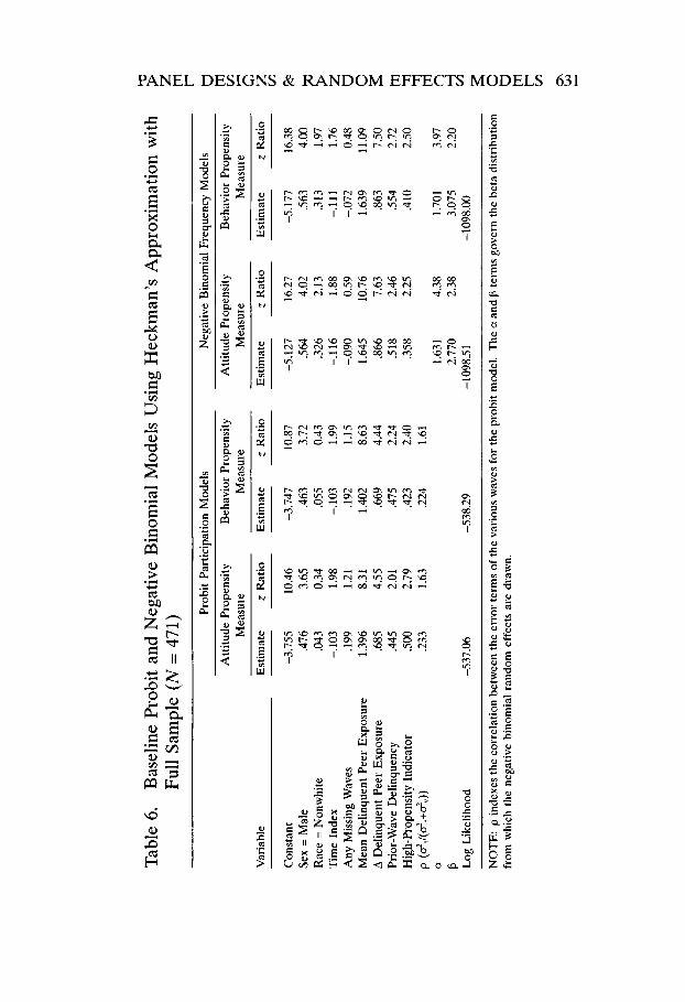
Tabl

e 6.

B

asel

ine

Prob

it an

d N

egat

ive

Bin

omia

l Mod

els

Usi

ng H

eckm

an’s

App

roxi

mat

ion

with

Fu

ll Sa

mpl

e (N

= 4

71)

Var

iabl

e

Con

stan

t Se

x =

Mal

e R

ace

= N

onw

hite

Ti

me

Inde

x A

ny M

issi

ng W

aves

M

ean

Del

inqu

ent

Peer

Exp

osur

e A

Del

inqu

ent

Peer

Exp

osur

e Pr

ior-

Wav

e D

elin

quen

cy

Hig

h-Pr

open

sity

Ind

icat

or

p (+

42,+

dv))

a P Lo

g Li

kelih

ood

~ ~~

~

Prob

it Pa

rtici

patio

n M

odel

s

Atti

tude

Pro

pens

ity

Beh

avio

r Pr

open

sity

Estim

ate

z R

atio

Es

timat

e z

Rat

io

-3.7

55

10.4

6 -3

.747

10

.87

,476

3.

65

,463

3.

12

.043

0.

34

.055

0.

43

-.I03

1.

98

-.I03

1.

99

.199

1.

21

.192

1.

15

1.39

6 8.

3 1

1.40

2 8.

63

.685

4.

55

.669

4.

44

.445

2.

01

.475

2.

24

,500

2.19

.4

23

2.40

,2

33

1.63

.2

24

1.61

Mea

sure

M

e as u

r e

-537

.06

-538

.29

Neg

ativ

e B

inom

ial

Freq

uenc

y M

odel

s

Atti

tude

Pro

pens

ity

Beh

avio

r Pr

open

sity

M

easu

re

Mea

sure

Est

imat

e z

Rat

io

Est

imat

e z

Rat

io

-5.1

27

.564

.3

26

-.116

-.0

90

1.64

5 ,866

.518

.3

58

16.2

7 4.

02

2.13

1.

88

0.59

10

.76

7.63

2.

46

2.25

-5.1

77

16.3

8 56

3 4.

00

.313

1.

97

-.111

1.

76

-.072

0.

48

1.63

9 11

.09

,863

7.

50

.554

2.

72

.4 10

2.

50

1.63

1 4.

38

1.70

1 3.

97

2.77

0 2.

38

3.07

.5

2.20

-1

098.

00

-1 09

8.5 1

NO

TE

: p

inde

xes

the

corr

elat

ion

betw

een

the

erro

r ter

ms

of t

he v

ario

us w

aves

for

the

prob

it m

odel

. T

he a

and

P te

ims g

over

n th

e be

ta d

istri

butio

n fr

om w

hich

the

nega

tive

bino

mia

l ra

ndom

eff

ects

ale

dra

wn.

M r

U

0 K Y

632 BRAME ET AL.

their magnitude is substantially smaller than what we originally reported. As expected from the simulation evidence presented above, the effect of ignoring initial conditions is to bias positively the estimate of the effect of the lagged outcome variable.'*

For the event-count outcomes in Tables 5 and 6, the estimated effects of prior offending activity continue to be positive and statistically significant but their magnitudes are sharply diminished from the values we first reported (see Tables 3 and 4). In our original negative binomial models, we reported that the effect of prior on current offending was .959 and .984 for the attitude and behavior measures, respectively. With the Heckman approximation, however, these coefficients are reduced to .400 (for the complete data) and SO0 (when cases with some periods of missing data are included), although they remain statistically significant.

In our original analysis, we reported that the probit coefficient for the effect of delinquent peers on subsequent behavior was approximately .900, and statistically significant. Moreover, an examination of a criminal propensity by delinquent peer exposure interaction indicated that the effect of delinquent peers was comparable for those with high and low criminal propensity.

Tables 5 and 6 report mean-centered revised estimates of the effects of delinquent peer exposure. A key feature of these results is the presence of two estimates of delinquent peer exposure effects. The first estimate rep- resents the effect of individual differences in average levels of delinquent peer exposure over the entire survey period of four years. Our primary interest in the delinquent peer exposure variable, however, is in the effects of year-to-year changes in delinquent peer exposure on offending activity. As Tables 5 and 6 suggest, the estimated effects of delinquent peer exposure are reduced somewhat from the values we originally reported. While shifts in delinquent peer exposure are strongly related to self-reported levels of criminal activity, our conclusion is that the mean-centering procedure of Horney et al. (1995) leads to an (appropriately) more conservative estimate of these effects.

In Tables 7 and 8, we present the parameter estimates associated with an interactive specification. In this analysis, we relax the constraint that delinquent peer exposure and prior offending effects are the same across

18. It is important to keep in mind, however, that our simulation evidence indicated that the Heckman approximation provides a negatively biased estimate of the true effect of lagged y. Our reported estimate for prior offending with this approximation, then, is a conservative one, and we do not know the precise magnitude of the attenuation. As we have suggested, the advantage of the Heckman approximation is not that it provides an unbiased estimator, but that it provides a less biased estimator than either ignoring the initial-conditions problem completely or applying some other "fix" (such as assigning the first lag y to zero for everyone).


the high and low antisocial propensity groups. In our previous analysis we found that the effects of these variables were similar for both groups. As Tables 7 and 8 suggest, these conclusions continue to hold for the random- effects probit specifications. Our random-effects count data estimator that invokes the behavioral measure of antisocial propensity also leads us to this conclusion. Despite these important similarities, however, the results no longer speak with one voice. When we employ the attitude-based measure of antisocial propensity in the count data estimator, the effect of prior criminal activity on future criminal activity is virtually zero among those with high antisocial propensity, but it is positive and statistically significant for the balance of the population.19 Contrary to our original results, this is exactly what typological theorists like Moffitt and Patterson would predict.

DISCUSSION AND CONCLUSIONS

Collectively, both our simulation results and our examination of the previously reported findings of Paternoster and Brame (1997) converge to suggest that the initial-conditions problem must be given careful consider- ation by researchers using panel data. When initial conditions are not ade- quately resolved, a bias favoring a dynamic explanation of behavior is propagated throughout the model to affect the estimated coefficients on lagged dependent variables, the time-varying and time-stable explanatory variables, and the correlation of the error term over time. In addition, bias is also caused when unobserved heterogeneity is correlated with any time- varying explanatory variables in the model. This bias also favors a dynamic explanation of crime. The bias due to the failure to observe initial conditions appears to be larger than the bias due to the zero-covariance problem. This finding has obvious implications for some of the literature in this area because researchers have employed a lagged measure of offending as a proxy for dynamic causal processes.

The Paternoster and Brame (1997) article discussed above and a similar study by Nagin and Paternoster (1991) used self-reported data from general population surveys and found strong evidence that prior offending was a key correlate of future crime. In contrast, work by Nagin and Far- rington (1992b) and Paternoster et. al. (1997) using official data from higher risk samples found little evidence for this conclusion. Paternoster and Brame (1997) speculated that these different results across studies could support a typological theory of crime posited by Moffitt (1993) or

19. There was some suggestion of this pattern in our original analysis but it was not statistically significant at conventional significance levels. Importantly, this interaction does not appear to hold with the same strength when the analysis is confined only to cases with valid data for all four waves.

Tabl

e 7.

Pr

obit

and

Neg

ativ

e B

inom

ial M

odel

s w

ith I

nter

actio

n Te

rms

Usi

ng H

eckm

an's

App

roxi

mat

ion

on C

ompl

ete

Dat

a Sa

mpl

e (N

= 3

90)

Prob

it Pa

rtici

patio

n M

odel

s

Atti

tude

Pro

pens

ity

Beh

avio

r Pr

open

sity

M

easu

re

Mea

sure

Var

iabl

e E

stim

ate

z R

atio

Es

timat

e 7

Rat

io

Con

stan

t Se

x =

Mal

e R

ace

= N

onw

hite

Ti

me

Inde

x M

ean

Del

inqu

ent

Peer

Exp

osur

e A

Del

inqu

ent P

eer

Expo

sure

Pr

ior-

Wav

e D

elin

quen

cy

Hig

h-Pr

open

sitv

Ind

icat

or

Inte

ract

ion

Teim

s Pr

open

sity

x M

ean

Del

. Pee

1 Ex

p.

Prop

ensi

ty x

A D

el. P

eer

Exp.

Pr

open

sity

x P

rior

Del

inqu

ency

p

(a?,

/(u?,

+u!,,

))

a P Log

Like

lihoo

d

-3.5

91

.511

-.0

18

-.I18

1.30

1 ,7

79

.423

,3

56

,203

-.0

94

-.491

,2

57

466.

47

9.36

3.

53

0.13

2.

05

6.98

4.

21

1.68

0.

47

0.47

0.

24

0.81

1.

71

-3.4

58

,535

-.0

11

-. 12

2 1.

245

.776

.3

19

-1.4

40

1.02

0 -.0

75

,279

,2

47

-466

.56

9.91

3.

84

0.07

2.

16

7.30

4.

22

1.32

I .0

6

1.35

0.2 1

0.

55

1.71

Neg

ativ

e B

inom

ial

Freq

uenc

y M

odel

s

Atti

tude

Pro

pens

ity

Beh

avio

r Pr

open

sity

M

easu

re

Mea

sure

Estim

ate

z R

atio

E

stim

ate

z R

atio

-5.2

59

,824

,0

96

1.96

6 1.

259

,434

2.

228

-.I46

-.843

-.0

93

-.515

1.85

7 1.

567

-861

.28

13.0

2 4.

59

0.48

2.

07

9.05

6.

04

1.90

1.

92

1.33

0.

25

0.81

4.98

2.

56

-5.1

07

,826

,1

15

-.I60

1.

952

1.26

5 ,2

63

1.65

1

-.822

-.0

49

.314

1.82

8 1.

480

-864

.55

12.9

1 4.

68

0.56

2.

33

9.07

6.

54

I .09

1.10

1.04

0.

12

0.57

5.00

2.

48

NO

TE

: p

inde

xes

the

corr

elat

ion

betw

een

the

erro

r ter

ms o

f th

e va

rious

wav

es fo

r th

e pr

obit

mod

el.

The

a an

d fr

om w

hich

the

nega

tive

bino

mia

l ra

ndom

eff

ects

are

dra

wn.

te

rms g

over

n th

e be

ta d

istri

butio

n

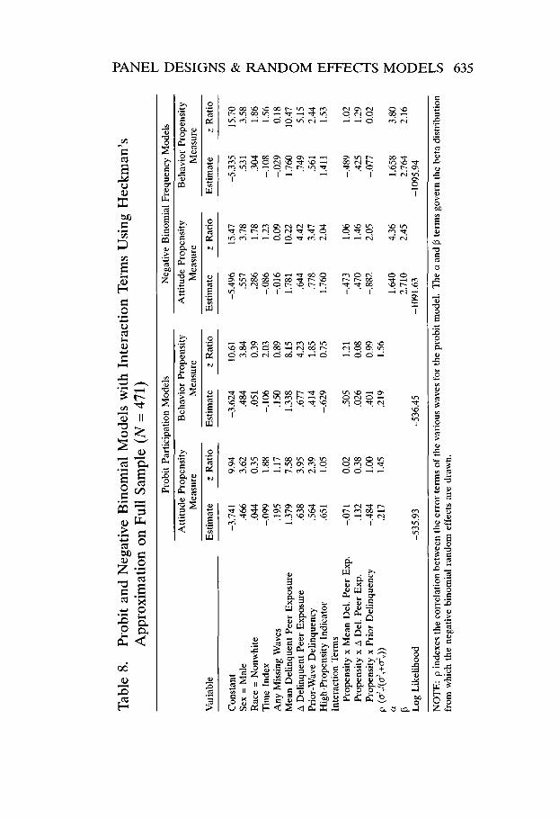
Tabl

e 8.

Pr

obit

and

Neg

ativ

e B

inom

ial

Mod

els

with

Int

erac

tion

Term

s U

sing

Hec

kman

's A

ppro

xim

atio

n on

Ful

l Sam

ple

(N =

471

)

Var

iabl

e

Con

stan

t Se

x =

Mal

e R

ace

= N

onw

hite

Ti

me

Inde

x A

ny M

issi

ng W

aves

M

ean

Del

inqu

ent P

eer

Expo

sure

A

Del

inqu

ent

Peer

Exp

osur

e Pr

ior-

Wav

e D

elin

quen

cy

Hig

h-Pr

open

sity

Ind

icat

or

Inte

ract

ion

Teim

s Pr

open

sity

x M

ean

Del

. Pee

r Ex

p.

Prop

ensi

ty x

A D

el. P

eer

Exp.

Pr

open

sity

x P

rior

Del

inqu

ency

p

(&4

U2

,+&

"))

P a Log

Like

lihoo

d

Prob

it Pa

rtici

patio

n M

odel

s A

ttitu

de P

rope

nsity

B

ehav

ior

Prop

ensi

ty

Mea

sure

M

easu

re

Est

imat

e z

Rat

io

Est

imat

e z

Rat

io

-3.7

41

9.94

-3

.624

10

.61

.466

3.

62

.484

3.

84

.044

0.

35

.051

0.

39

-.099

1.

88

-.lo6

2.

03

.195

1.

17

.150

0.

89

1.37

9 7.

58

1.33

8 8.15

.638

3.

95

.677

4.

23

,564

2.

39

.414

1.85

,651

1.

05

-.629

0.

75

-.07

1 0.

02

.SO5

1.21

.I

32

0.38

,026

0.08

,484

1.

00

.401

0.

99

.217

1.

45

.219

1.

56

-535

.93

-536

.45

Neg

ativ

e B

inom

ial

Freq

uenc

y M

odel

s

Atti

tude

Pro

pens

ity

Beh

avio

r Pr

opei

isity

M

easu

re

Mea

sure

Est

imat

e z

Rat

io

Est

imat

e z

Rat

io

-5.4

96

15.4

7 -5

.335

15

.70

.557

3.

78

S31

3.58

,286

1.

78

,304

1.

86

-.086

1.

23

-.lo

8 1.

56

:016

0.09

-.0

29

0.18

1.

781

10.2

2 1.

760

10.4

7 .6

44

4.42

.7

49

5.15

.7

78

3.47

.5

61

2.44

1.

760

2.04

1.

411

1.53

-.473

1.

06

-.489

1.

02

.470

1.

46

.425

1.

29

-.882

2.0

5 -.0

77

0.02

1.64

0 4.

36

1.65

8 3.

80

2.71

0 2.

45

2.76

4 2.

16

-109

1.63

-1

095

.94

NO

TE:

p in

dexe

s the

cor

rela

tion

betw

een

the

erro

r tei

ms

of t

he v

ario

us w

aves

for t

he p

robi

t mod

el.

The

a an

d p

term

s go

vern

the

beta

dis

tribu

tion

from

whi

ch th

e ne

gativ

e bi

nom

ial

rand

om e

ffec

ts a

re d

raw

n.

z 0

u

o\

w

c/I

BRAME ET AL.

Patterson (1993). or could be caused by differences between self-report and official data.

Our current analysis now suggests a third possible explanation. Studies with strong results supporting dynamic criminological theories may have overstated the importance of dynamic factors. The reported coefficient estimates for dynamic factors from these studies could be biased because of problems with initial conditions. Both the Paternoster and Brame (1997) and Nagin and Paternoster (1991) studies violate the initial-conditions assumption. These studies are based on self-reported involvement in minor forms of delinquent behavior within a sample of conventional youth, a nontrivial proportion of whom were already involved in offending at the time of the first measurement period. In contrast, the studies that found evidence more supportive of static theories (Nagin and Farrington, 1992a, 1992b; Paternoster et al., 1997) do not violate the initial-conditions assumption. It is important to keep in mind, however, that evidence in this analysis and others clearly continue to suggest that dynamic factors such as delinquent peer exposure are important.

A logical and perhaps immediate response to the estimation problems discussed here might be to avoid specifying models that include lagged offending as an explanatory variable. Since lagged offending has been used as a proxy for other dynamic processes that may have an impact on future offending, and since there is evidence that dynamic processes are important, inclusion of other variables that more accurately reflect the dynamic processes of interest may be more interesting. Time-varying variables other than prior offending may also be valuable from a technical standpoint since the effects of these kinds of covariates can be consistently estimated without appealing to the initial-conditions assumption.

A problem with such an approach is that the failure to include the lagged outcome variable may itself distort matters because there are compelling theoretical reasons to retain it. Nagin and Paternoster (1991) have previously suggested several theoretical routes whereby past offending activity can have an important causal effect on future offending activity. Akers’ (1985) learning theory, for example, predicts that crime can be a positive and rewarding experience for some (netting money, excitement, status from peers), leading to additional crime. Experiencing crime as a positive reinforcement will, other things being equal, lead one to revisit it. A special case of this is Jack Katz’s (1988) notion that crime provides its participants with “sneaky thrills”-thereby seducing them into continued action. The argument that crime has its own rewards is also central to labeling theory’s explanation of secondary deviance (Lemert, 1967).

The problem with the correlation between dynamic €actors and unobserved heterogeneity is more easily addressed. Separating the variable into its within-individual and between-individual components is both


straightfoiward and intuitive. Future work that uses random-effect-like estimation on panel data should begin to report results using this type of decomposition.

We think that another line of future research concerns sources of omitted variable bias in panel analysis not covered by our current work. As we mentioned above, there are three types of omitted variable bias in studies like the kind we discuss here. One type of bias occurs when time-constant omitted variables are correlated with time-constant included variables (type 1). A second type of bias, which was our concern here, occurs when time-constant omitted variables are correlated with time-varying included variables (type 2). Finally, a third type of omitted variable bias occurs when time-varying omitted variables are correlated with time-varying included variables (type 3). Type 1 bias is generic and not unique to panel analysis, and it is very difficult to resolve. Type 3 bias, we think, is more tractable and should be the subject of additional research. For our part, we are continuing to try to resolve these issues and extend an invitation for others to join us.

REFERENCES

Akers, Ronald L. 1985 Deviant Behavior: A Social Learning Approach. 3d ed. Belmont, Calif.:

Wadsworth.

Using panel data to estimate the effects of events. Sociological Methods and Research 23:174-199.

Criminal Careers and “Career Criminals.” Washington, D.C.: National Academy Press.

Hierarchical Linear Models: Applications and Data Analysis Methods. Newbury Park, Calif.: Sage.

Assessing stability and change in criminal offending: a comparison of random effects, semiparametric, and fixed effects modeling strategies. Journal of Quantitative Criminology 15:3342.

Allison. Paul D. 1994

Blumstein, Alfred, Jacqueline Cohen, Jeffrey A. Roth. and Christy A. Visher (eds.) 1986

Bryk. Anthony S. and Stephen W. Raudenbush 1992

Bushway, Shawn, Robert Brame, and Raymond Paternoster 1999

Corcoran, Martha and Mary S. Hill 1985 Reoccurrence of unemployment among young adult men. Journal of

Human Resources 20165-183.

Donovan, John E. and Richard Jessor 1985 Structure of problem behavior in adolescence and young adulthood. Jour-

nal of Consulting and Clinical Psychology 532390-904.

Explaining Delinquency and Drug Use. Beverly Hills, Calif.: Sage. Elliott, Delbert S., David Huizinga, and Suzanne S. Ageton

1985

638 BRAME ET AL.

Elliott, Delbert S., David Huizinga, and Scott Menard

Farrington, David F. 1989 Multiple Problem Youth. New York: Springer-Verlag

Age and crime. In Michael H. Tonry and Norval Moms (eds.), Crime and Justice: A Review of Research. Vol. 7. Chicago: University of Chicago Press.

1986

Fishman, George S. 1996 Monte Carlo: Concepts, Algorithms, and Applications. New York:

Springer-Verlag.

A General Theory of Crime. Stanford, Calif.: Stanford University Press.

Mathematical Criminology. New Brunswick, N.J.: Rutgers University Press.

1995 LIMDEP, Version 7.0: User’s Manual. Bellport, N.Y.: Econometric

1997

Gottfredson, Michael R. and Travis Hirschi

Greenberg, David F.

Greene. William H.

1990

1979

Software. Econometric Analysis. 3d ed. Upper Saddle River, N.J.: Prentice-Hall.

Econometric models for counted data with an application to the patents- R&D relationship. Econmetrica 523909-938.

The incidental parameters problem and the problem of initial conditions in estimating a discrete time-discrete data stochastic process. In Charles F. Manski and David McFadden (eds.), Structural Analysis of Discrete Data with Econometric Applications. Cambridge, Mass.: MIT Press.

Causes of Delinquency. Berkeley: University of California Press. Review of Delinquency and Drug Use. Criminology 25:193-201.

Hirschi, Travis and Michael R. Gottfredson Control theory and the life-course perspective. Studies on Crime and Crime Prevention 4131-142.

Criminal careers in the short-term: Intra-individual variability in crime and its relation to local life circumstances. American Sociological Review 60:655-673.

Analysis of Panel Data. New York: Cambridge University Press.

Seductions of Crime: Moral and Sensual Attractions in Doing Evil. New York: Basic Books.

Linear Panel Analysis: Models of Quantitative Change. New York: Aca- demic Press.

Unifying Political Methodology: The Likelihood Theory of Statistical Infer- ence. New York: Cambridge University Press.

Hausman, Jerry, Bronwyn H. Hall. and Zvi Griliches 1984

Heckman, James J. 1981

Hirschi, Travis 1969 1987

1995

Homey, Julie, D. Wayne Osgood, and Ineke H. Marshall 1995

Hsiao, Cheng 1986

Katz, Jack 1988

Kessler, Ronald C. and David F.Greenberg 1981

King, Gary 1989


Land. Kenneth C. and Daniel S. Nagin 1996 Micromodels of criminal careers: A synthesis of the criminal careers and life

course approaches via semiparametric mixed Poisson regression models, with empirical applications. Journal of Quantitative Criminology 12~163-190.

Land, Kenneth C.. Patricia L. McCall, and Daniel S. Nagin 1996 Comparison of Poisson, negative binomial, and semiparametric mixed Pois-

son regression models with empirical applications to criminal careers data. Sociological Methods and Research 24:387441.

Turning points in the life course: Why change matters to the study of crime. Criminology 31:301-325.

Trajectories of change in criminal offending: Good marriages and the desistance process. American Sociological Review 63:225-238.

Human Deviance. Social Problems, and Social Control. Englewood Cliffs, N.J.: Prentice-Hall.

Panel data and models of change: A comparison of first difference and conventional two-wave models. Social Science Research 1 4 80-101.

1990 Toward a developmental criminology. In Michael H. Tonry and Norval Moms (eds.), Crime and Justice: An Annual Review of Research. Vol. 12. Chicago: University of Chicago Press.

Random coefficient models. In Gerhard Arminger, Clifford C. Clogg, and Michael E. Sobel (eds.), Handbook of Statistical Modeling for the Behav- ioral and Social Sciences. New York: Plenum.

1987 Limited dependent variable models using panel data. Journal of Economic Resources 22:307-338.

1993 The Econometrics of Panel Data. Vols. 1 and 2. Brookfield, Vt.: E. E. Elgar.

Moffitt, Teme E.

h u b , John H. and Robert J. Sampson 1993

Laub, John H., Daniel S. Nagin, and Robert J. Sampson 1998

Lemert. Edwin M. 1967

Liker, Jeffrey K., Sue Augustyniak, and Greg J. Duncan 1985

Loeber, Rolf and Marc LeBlanc

Longford, Nicholas T. 1995

Maddala, G. S.

1993 Adolescence-limited and life-course-persistent antisocial behavior: A developmental taxonomy. Psychological Review 100:674-701.

The onset and persistence of offending. Criminology 30501-523. The stability of criminal potential from childhood to adulthood. Criminol-

Nagin. Daniel S. and David P. Farrington 1992a 1992b

O ~ Y 30235-260. Nagin, Daniel S. and Kenneth C. Land

1993 Age, criminal careers, and population heterogeneity: Specification and estimation of a nonparametric mixed Poisson model. Criminology 31:327-359.

On the relationship of past and future participation in delinquency. Crimi- nology 29163-190.

Nagin, Daniel S. and Raymond Paternoster 1991

BRAME ET AL.

1994 Personal capital and social control: The deterrence implications of a theory of individual differences in criminal offending. Criminology 32581-606.

Nagin, Daniel S., David P. Farrington. and Terrie E. Moffitt 1995 Life-course trajectories of different types of offenders. Criminology

33:111-139.

Osgood, D. Wayne, Lloyd D. Johnston, Patrick O’Malley, and Jerald G. Bachman 1988 The generality of deviance in late adolescence and early adulthood. Ameri-

can Sociological Review 53:Sl-93.

Paternoster, Raymond and Robert Brame 1997 Multiple routes to delinquency? A test of developmental and general theo-

ries of crime. Criminology 35:49-84.

Paternoster, Raymond, Charles W. Dean, Alex Piquero, Paul Mazerolle, and Robert

Generality, continuity and change in offending. Journal of Quantitative Criminology 13231-266.

Brame 1997

Patterson. Gerald R. and Karen Yoerger 1993 Developmental models for delinquent behavior. In Sheilagh Hodgins (ed.),

Mental Disorder and Crime. Newbury Park, Calif.: Sage.

Career criminal research. In Norval Moms and Michael H. Tonry (eds.), Crime and Justice: An Annual Review of Research. Chicago: University of Chicago Press.

Petersilia. Joan 1980

Robins, Lee N. 1966 1978

Deviant Children Grown Up. Baltimore: Williams & Wilkins. Sturdy childhood predictors of adult antisocial behavior. Psychological Medicine 8:611-622.

Rowe, David C. and Daniel J. Flannery 1994 An examination of environmental and trait influences on adolescent delin-

quency. Journal of Research in Crime and Delinquency 31:374-389.

Saltzman, Linda S., Raymond Paternoster, Gordon P. Waldo, and Theodore Chiricos Deterrent and experiential effects: The problem of causal order in percep- tual deterrence research. Journal of Research in Crime and Delinquency

1982

18: 172-189.

Sampson, Robert J. and John H. Laub 1992 Crime and deviance in the life course. Annual Review of Sociology

1993 Crime in the Making: Pathways and Turning Points Through Life. Cam- bridge, Mass.: Harvard University Press.

1995 Understanding variability in lives through time: Contributions of life-course criminology. Studies on Crime and Crime Prevention 4:143-158.

1997 A life-course theory of cumulative disadvantage and the stability of delinquency. In Terence B. Thornbeny (ed.), Developmental Theories of Crime and Delinquency. New Brunswick, N.J.: Transaction Publishers.

18~63-84.

Wilson, James Q. and Richard Hermstein 1985 Crime and Human Nature. New York Simon & Schuster.


Robert Brame is an Assistant Professor in the Department of Criminology and Crimi- nal Justice at the University of Maryland. His interests include the study of criminological theory and applied statistics. Shawn Bushway is an Assistant Professor in the Department of Criminology and Crimi- nal Justice at the University of Maryland. Work on this paper was completed while he was a post-doctoral fellow for the National Consortium on Violence Research at the University of Maryland. His research interests include the relationship between work and crime, statistical methods for use with panel data, desistance, and developmental criminology. Raymond Paternoster is Professor of Criminology at the University of Maryland and a Fellow with the National Consortium on Violence Research. His research interests include the testing of criminological theory and quantitative methods in criminology.

642 BRAME ET AL.

on the use of panel research designs and random effects models to investigate static and dynamic...

Documents