On the Monetization of Mobile Apps

Gil Appel

Marshall School of Business, University of Southern California

gappel@marshall.usc.edu

Barak Libai

Arison School of Business, Interdisciplinary Center, Herzliya

libai@idc.ac.il

Eitan Muller

Stern School of Business, New York University

Arison School of Business, Interdisciplinary Center, Herzliya

emuller@stern.nyu.edu

Ron Shachar

Arison School of Business, Interdisciplinary Center, Herzliya

ronshachar@idc.ac.il

January 2019

We would like to thank Roland Rust, SE and reviewers, Eyal Biyalogorsky, Anthony Dukes,

Daria Dzyabura, and Oded Koenigsberg for a number of helpful comments and suggestions.

1

On the Monetization of Mobile Apps

Abstract

Though the mobile app market is substantial and growing fast, most firms struggle to monetize

apps profitably. Monetizing apps is done in two ways: a) selling advertising space within a free

version of the app, and b) selling a paid version, termed freemium or in-app purchase strategy. In

this paper, we present a framework for monetization of mobile apps, using two central empirical

regularities concerning the relationship between users and their mobile apps: a) Uncertainty:

While consumers have some prior knowledge of their fit with the app, they remain uncertain

regarding their exact utility until they are using it; and b) Satiation: The utility of using the app

may decrease with time. While work on the monetization of digital goods has largely overlooked

the role of satiation and the consequent retention issues, we show that in combination with

uncertainty, it elucidates the role of the segments of consumers that download the free vs. paid

version of the app, and how to balance these two segments so as to monetize mobile apps. We

encounter two distinct scenarios: In the first, advertising drives most of the revenues; while in the

second, revenues are driven by the paid version of the app. We explain how uncertainty and

satiation affect the prevalence of the respective scenarios and impact the share of revenues from

the paid vs free version of the app. We also demonstrate that a firm can profit from offering a

free version with ads even if advertisers are not paying for these ads. In other words, the firm

benefits from offering a “damaged good” version of the app that includes ads, even if this

version is free to consumers, and the advertisers are not paying for the ads.

Keywords: advertising; freemium; mobile apps; online strategy; pricing; retention; satiation

2

1. Introduction

The number of mobile apps offered to consumers is rising rapidly, and by 2018, consumers

could choose among nearly six million apps in Google or Apple stores (Statista 2018). Industry

reports indicate that over 90% of mobile apps start as free, over 90% of the profits from mobile

apps come from apps that began as free, and that the share of free apps is expected to grow

(AppBrain 2018). Although these apps are “free”, market size is notable, at more than $80 billion

in 2017 and expected to almost double by 2022 (Cheney and Thompson 2018). The largest app

category is mobile games, whose revenues reached $70 billion in 2018, exceeding both video

console games and PC games (Wijman 2018).

Monetizing apps is mainly done in two ways: a) selling advertising space within a free

version of the app, and b) selling a paid version, or an in-app purchase strategy that offers

additional features for pay (Needleman 2016). As app creators struggle to remain profitable, the

question of choosing the correct business model and marketing mix becomes more pressing

(Natanson 2016). While advertising and pricing decisions have always been interwoven

(Assmus, Farley, and Lehmann 1984), in mobile apps, the interrelationship is magnified

significantly due to the specific segments that download each version of the app. Potential users

consider adopting the app in its two versions – free, and paid – and make these decisions over

time (Gu, Kannan, and Ma 2018). Indeed, many “sample” the free version while considering the

paid version (Deng, Lambrecht, and Liu 2018).

In this paper we present a framework for optimal app management in this complex

environment. We do so by looking at two aspects of app monetization that should be jointly

taken into account when considering marketing of mobile apps: satiation, and uncertainty.

Satiation. Customer retention is a key issue confronting the mobile apps industry (Jacobson

3

2018). Mobile app retention rates are typically much lower than observed retention rates for

classic products: Industry reports suggest that across all categories, over 70% of all app users

may churn within 90 days (Perro 2018). This introduces additional complexity into the decision

making, as the user who is targeted by advertising might have churned already in early periods of

the app life cycle. Thus, pricing and advertising decisions have a direct effect on the number of

users in each segment in both the current and future periods.

Low retention rates in the industry at large can be related to low switching costs and the

large and growing selection in the apps stores. At the individual level, marketers realize that

churn is closely related to declining engagement over time, which lowers users’ utility from apps

(AppsFlyer 2017). From a behavioral standpoint, such decline is consistent with abundant

evidence on satiation’s role in consumption patterns of products, hedonic products in particular

(Galak, Kruger, and Loewenstein 2013; Sevilla, Zhang, and Kahn 2016; Galak and Redden

2018). It is well recognized that repeated consumption of the same item over time is likely to

produce a decline in liking even for a positive experience, and in turn reduction and cessation of

usage. Therefore, under satiation, customer satisfaction will not necessarily lead to higher

revenue, as consumer lifetime value gradually declines (Voss, Godfrey, and Seiders 2010).

Satiation is thus a threat to the firm’s ability to generate future profits from its customers.

It is thus not surprising that satiation has been found to affect the consumption behavior of

mobile apps such as games (Han, Park, and Oh 2016; Hui 2017). However, the extent of the

phenomenon may differ considerably among app categories that likewise vary considerably in

their retention rates (App Annie 2016). The app research firm Flurry, for example, found that the

high-retention categories are health and fitness, weather, magazines, and business and finance;

while categories such as action games, sports, family, entertainment, and puzzles have much

4

lower retention probabilities (Klotzbach 2016). This difference may be thus related to the extent

to which apps are perceived more as hedonic vs utilitarian (Schulze, Schöler, and Skiera 2014).

Uncertainty. While apps are clearly not the only product where uncertainty affects decision, few

are the markets where consumers face such an extensive choice with relatively little product

knowledge. This is due to the sheer number of apps available and the general absence of

advertising budgets for such low-ticket items. Thus, while consumers have some prior

knowledge of their fit with a given app, they remain uncertain about their exact match-utility

until they are using it. Consequently, the firm has to design two versions – paid, and free –

knowing that some consumers will sample the product and decide about purchasing either

version in future periods once uncertainty is resolved as a result of the sampling procedure.

We show how monetization policy creates the market reality of paid and free apps, taking

into account the joint effect of customer uncertainty and satiation. The equilibria in our setting

result from consumers maximizing utility by choosing free or paid versions, and the app

producer maximizing profits by optimally choosing price and advertising. We see that this

setting in fact leads to two distinct scenarios: In the first, advertising drives most of the revenues;

while in the second, revenues are driven by the paid version of the app. We will demonstrate

how uncertainty and satiation affect the prevalence of the respective scenarios.

In particular, our analysis elucidates the importance of satiation in the market. Satiation’s

role is notable given that academic discussion of app monetization to date has largely overlooked

the relevance of user duration with the app. We show that the optimal prevalence of free versus

paid apps is related to the level of satiation: When satiation increases, initially, the paid version’s

share of the app decreases; then, when satiation is high enough, the firm offers only the ad-

supported version of the app. The following analysis helps us to understand how and why this

5

happens, and how persistence also creates value through its effect on advertising and price.

We also show that the firm benefits from offering a free version of the app that contains ads

even if advertisers are not paying for these ads. The logic behind the production of this

“damaged good” is that the free version acts as a sample that enables consumers to learn their fit

with the app. The firm would rather add advertising to this version in order to keep the

consumers who derive high value from the app away from the sample, and push them toward the

paid version. Overall, our analysis demonstrates how the respective shares of paid and free apps

are a function of a complex process that combines app features and the marketing mix to yield

user utility. Managers need to understand this process in order to set realistic expectations,

understand the impact of various parameters, and design strategies to increase profitability.

2. Related literature

Our work is relevant to research efforts aiming at understanding firm behavior in free digital

markets. Research in this area has largely focused on the choice between content and advertising

in the context of media markets, where the basic tradeoff is that moving from an advertising-only

revenue model to charging for content, may reduce usage and thus hurt advertising revenues

(Lambrecht et al. 2014). Specifically, our work is related to recent calls for better understanding

of freemium product design to maximize customer lifetime value (Kannan and Li 2017).

Empirical results regarding the consequences of such a choice vary. Profitability in such

contexts may depend on factors such as the type of promotions used (Pauwels and Weiss 2008),

temporal changes in demand (Lambrecht and Misra 2016), and users’ ability to bring in new

business through referrals (Lee, Kumar, and Gupta 2017). It had been also suggested that the

existence of free apps may affect the speed of paid alternatives’ growth (Arora, Hofstede, and

Mahajan 2017; Deng, Lambrecht, and Liu 2018). Analytically, noticeable effort has centered on

6

the questions of profit from content vs. advertising in two-sided media markets such as

newspapers (Halbheer et al. 2014). The tradeoff between paid content and advertising may

depend on competitive intensity (Godes, Ofek, and Sarvary 2009), consumer heterogeneity in

willingness to pay (Prasad, Mahajan, and Bronnenberg 2003), or the extent to which consumers

dislike advertising (Tåg 2009).

Viewing the use of a free product as a sampling mechanism, recent work has suggested that

advertising’s effectiveness, coupled with consumers’ expectations regarding quality, can

determine which revenue source firms should focus on in attempting to enhance profitability

(Halbheer et al. 2014). Moreover, it has been shown that the appeal of the free option is

influenced by the effectiveness of word of mouth (Niculescu and Wu 2014), and by quality and

other design parameters (Li, Jain, and Kannan 2019). These research efforts, however, do not

consider customer satiation’s role and its effect on retention in the subsequent market state.

Our work is also relevant to the literature on product line design (Moorthy 1984; Moorthy

and Png 1992; Biyalogorsky and Koenigsberg 2014; Gu, Kannan, and Ma 2018). The main

driving force behind product line design and pricing is the fact that consumers derive differing

valuations from the product’s attributes. The firm knows the distribution of preferences, yet not

individual preferences, and thus cannot engage in standard monopoly (first-degree) price

discrimination. Instead, it offers a line of products and relies on self-selection of consumer

segments thereto, thereby permitting partial discrimination among consumers. This self-selection

process relies on incentive-compatibility constraints that deter one segment from purchasing the

“wrong” product that was designed for another segment.

As Gu, Kannan, and Ma (2018) demonstrate, questions of app market planning, for example

extending the premium product line, can be analyzed from a product line standpoint. Indeed, our

7

model features this type of price discrimination, where the firm offers two product versions

(paid, and free), and consumers self-select, where the low-valuation consumers download the

free version (with the nuisance of ads), and the high-valuation consumers choose the paid

version. What complicates the analysis considerably is the introduction of uncertainty: As

Biyalogorsky and Koenigsberg (2014) indicated, uncertainty complicates the design problem of

developing products that satisfy the incentive-compatibility constraints. In our case, the firm has

to design both versions, knowing full well that some consumers will sample the product and

decide about purchasing either version in the subsequent period, once uncertainty is resolved.

Given our emphasis, our work is relevant to the avenue of research that addresses customer

retention’s consequences (Libai, Muller, and Peres 2009; Ascarza et al. 2018), and how optimal

retention efforts may differ based on market characteristics (Musalem and Joshi 2009; Shin and

Sudhir 2012; Subramanian, Raju, and Zhang 2013). In the context of online behavior,

researchers have considered the antecedents of users’ tendencies to stick with an app (Hsu and

Lin 2016). Yet the dynamics of how satiation, and consequently retention, affect monetization in

free digital markets, have not been examined.

Finally, as the consumers in our setting learn about the app, our work addresses the demand-

side literature on consumers’ learning (Erdem et al. 1999; Iyengar, Ansari, and Gupta 2007). Our

learning structure is not on specific attributes of the app, but rather on the idiosyncratic utility

that the consumer can expect from experiencing the app, similar in spirit to Ackerberg (2003).

Free samples in technological products have been shown to be an effective way to convey

information, lowering consumers’ risk associated with adoption, and consequently accelerating

adoption (Foubert and Gijsbrechts 2016; Li, Jain, and Kannan 2019). Here we show how such

learning combines with post-adoption satiation to affect market outcomes.

8

3. The model

To clarify the exposition, we chose the following example of a mobile game of a popular

category: Role Playing Games (RPG). RPG is an app category intended for mobile devices,

distributed on either Google’s Play Store or Apple’s iOS App Store as either free, or paid1. The

game, Doom and Destiny, is designed in the 8-bit graphics style of Japanese RPG (JRPG) by

Italian developer Heartbit Interactive. The game tells the story of four nerds who get drawn into

a fantasy world. Mistaken for heroes, they must battle their way through an adventure in order to

defeat a villain. It contains nerdy humor and strong language, so that advocacy group and text

monitoring app SaferKid recommended 12+ as a safe age to play the game. The game was

launched on Android in 2013, and currently has over 500k installs and 70k reviews for the free

version, and over 50k installs and 18k reviews for the paid version. It is also quite popular, as for

example, the paid version is #9 in the US in the Role Playing category (as of November 2018). In

terms of the costs to consumers, in user time or out-of-pocket expenses, in the free version, an ad

appears every 3 minutes, covering the entire screen for 5 seconds; while the paid version costs

$4.99. The only difference between the two is lack of advertising in the paid version.

In the next subsection, we use Doom and Destiny as a running example in order to better

elucidate the main factors affecting consumers’ utility such as uncertainty, advertising, and price.

3.1 Uncertainty, advertising, and price

We begin by describing the factors affecting consumers’ utility such as uncertainty,

advertising, and price; then proceed with the formal utility maximization problem; and conclude

with the resultant demand and firm maximization.

1 The term “free” app is somewhat of a misnomer, as even the “free” version has a cost, i.e., the consumer pays with

her time by viewing advertising. However, for convenience’ sake, we refer to the ad-supported version as “free”.

9

Uncertainty. Although consumers might have some prior knowledge about the app, they remain

uncertain about the idiosyncratic utility they can expect from using the app (Morvinski, Amir,

and Muller 2017). In the above-described example of Doom and Destiny, judging from the

reviews, there’s uncertainty about the user’s match with the app until s/he begins playing the

game. The reason for this might be that the description is rather terse and generic: The user might

consider herself a nerd, yet cannot be sure that the humor fits or about the crudity of the

language, or some idiosyncrasies of the game’s technical aspects. Thus we find reviews that

state, “I didn’t expect this to be a gem…” and “…love the dialog, cursing included…”, and

“…new way to play with the control setup being something I’ve never used before…”

Product fit uncertainty is a major impediment to online markets in general (Hong and Pavlou

2014). Consumers’ uncertainty about apps is amplified, as the majority of apps have been

developed by small businesses with unknown reputations (Arora, Hofstede, and Mahajan 2017).

Market reports suggest that given the absence of monetary cost to download apps, consumer

learning often occurs post-adoption, rather than pre-adoption as in classic consumer markets

(Klotzbach 2016). Yet consumers are not entirely in the dark with respect to their match with any

given app. For example, some consumers know a-priori that they prefer “social games” over

“brain games”. However, as each app is unique, even after reading an app’s description,

consumers are uncertain about the fit between their preferences and the app.

The costs and benefits of advertising. The free version of the app is bundled with advertising.

Exposure to advertising is irksome to the consumer, arousing annoyance and irritation, and thus

the intensity of advertising (denoted by 𝛾) depreciates the consumer’s utility (Wilbur 2008).

Advertising creates inconvenience for the consumer in that it effectively reduces the level of

content that s/he can enjoy from the app, in addition to inflicting other costs, such as distraction

10

and opportunity cost of time, resulting in a negative effect on utility and retention (Tåg 2009;

Goldstein et al. 2014). Indeed, in Doom and Destiny, users have complained about the ads in

reviews such as: “…I’m thinking of buying the full game to get rid of those pesky ads…” and

“This game is awesome… though there were scientology ads which made confused deeply. [sic]”

As the aforementioned scientology advertising demonstrates, firms tend to have limited

control over ad content, which is typically outsourced to ad exchanges that match ads to apps

(e.g., Google’s Marketing Platform; Yahoo’s Flurry; OpenX). However, the firm can select the

level of advertising intensity, and thus Heartbit Interactive, for example, can decide to have an ad

every 2 minutes rather than every 3 in Doom and Destiny.

These additional ads come with a cost, though: Firstly, ad exchanges pay developers on a

cost-per-click basis. Posting more ads leads to lower click-through rates, leading to lower ad

conversion rate, and thus to lower revenues from advertising (Babu 2018). Moreover, there can

be a more general effect on the brand in general. Given the strong resentment of many

individuals toward ads in games (Lagace 2018), heavy advertising can harm the brand name such

that it interferes with firm’s ability to acquire customers and retain them. There is a limit to how

often a firm can advertise without causing such damage.

Paid version price. Consumers may choose to eliminate the annoyance of ads, for a price. The

firm offers a paid version of the app for a price p ≥ 0. If consumers choose to pay this price, the

ads are removed and the consumers enjoy the app’s full utility. Hence Heartbit Interactive can

decide to price Doom and Destiny at $3.99 rather than the current $4.99. As we show later,

choice of price and advertising levels has a profound effect on the size and revenues of the

consumer segments that download the paid vs the free version of the app.

11

Satiation and persistence. As discussed previously, satiation is expected to affect consumption

over time (Galak and Redden 2018). Our model considers satiation to be a feature of the app.

Various app-based factors may influence an app’s satiation level, including the app’s quality and

its ability to create consumer engagement, commitment, and trust (Hsu and Lin 2016). Market

studies suggest that observed retention rates (which follow the extent of satiation) depend on the

specific type of app, and on variety seeking and boredom on the part of the target market

(Klotzbach 2016).

Consistent with the customer duration literature that often highlighted retention rather than

churn, we define the fraction of the utility that is still experienced in the second period, and label

this parameter (denoted by 𝛿) the persistence parameter. Persistence is the opposite of satiation,

of course, as churn is to retention: the higher the persistence, the lower the satiation and the more

utility remains by the second period. Note that satiation (or persistence) reflects changes in utility

over time. While it is naturally a key antecedent of user retention, it is not the only one: Other

market factors, as we discuss here, may play a role in the final consumer decision. The actual

churn decision depends upon the overall utility, if it is negative.

In our example, while we do not have access to Doom and Destiny usage data, we can find

out the mobile games category’s average usage. In order to assess the level of persistence, we

make two assumptions2: Firstly, a “period” in our model is a week; and secondly, usage is a

reasonable proxy for utility. Under these assumptions, we utilize an Adjust Mobile Benchmark

Q3 2016 study (the latest available) to compute average usage, in minutes per day, of the first

and second week for Android users. This if we use the average usage time as a proxy for utility,

2 As this is just an example for computation of satiation, the assumptions are not inherent to our analysis, and are

used solely for this example. Nonetheless, both assumptions are reasonable: As industry reports indicate the time

frame used for these fast-moving games are either daily or weekly; and usage, while not perfect, might be a good

proxy for the engagement and therefore utility enjoyed by the player.

12

then the average time a user spends on a game is 15.3 minutes per day in the first week, and 8

minutes per day in the second, leading to a persistence parameter of 𝛿 =8

15.3= 0.53.

3.2 Consumer’s expected utility

In each period (𝑡 = 1,2) the user faces three alternatives with three corresponding utility levels:

(1) {

a) not use the app with resultant utility of 𝑢0,𝑡 = 0

b) use the free app with utility 𝑢𝑎,𝑡 = 𝜈𝛿𝑡−1(1 − 𝛾)

c) use the paid version of the app with utility 𝑢𝑝,𝑡 = 𝜈𝛿𝑡−1 − 𝑝𝐼{𝑡}

where 𝐼{𝑡} = 1 if the consumer bought the app in period t and 0 otherwise; 𝜈 is the experience

utility, 𝛾 is the intensity of advertising, and 𝛿 is the app persistence parameter. The utility gained

from the app is 𝑣 in the first period and 𝑣𝛿 in the second period. In the example given in the

previous subsection, if 𝑣 = 15.3 in the first period, then 𝑣𝛿 = 8 in the second (to simplify

notations, we normalize utility as we show later). Utility is multiplied by 1 − 𝛾 if the free version

is used. The indicator function I captures the fact that the price is paid only once. Note that 𝛾 and

𝛿 are bounded between 0 and 1.

Formalizing uncertainty. To capture uncertainty, we let it be additive, in that each consumer is

assigned a base utility of α, and then nature either adds or subtracts 휀 to or from α (with

probability of 1/2 to each option). Thus let 𝑣 = 𝛼 + 𝜇 where 𝑣 denotes the experience utility of

the app, 𝛼 the base utility – an attribute that is known ex-ante – and 𝜇 the match utility, a

horizontal attribute that is learned after use in the first period. This process is common

knowledge, and each consumer knows her own α, yet does not know whether nature added or

subtracted 휀 in her case. The distributional assumptions are that 𝜇 has a Bernoulli distribution

with parameter 𝑝 =1

2 on {−휀, 휀}, where 휀 ≥ 0, and that α and 휀 are distributed uniformly in the

13

interval (0,1). Thus, the parameter 휀 represents the degree of uncertainty that the consumer faces

with respect to her true base utility. This uncertainty is resolved when the consumer uses the app,

irrespective of whether she uses its free or paid version.

Next, we formalize the consumer’s utility when using the app’s paid and free versions.

Consumer chooses paid version. Note that when forming expectations, the consumer takes into

account the consequences of her choices in the first period on her state in the second in two

ways: Firstly, using the app resolves uncertainty, and the consumer knows whether his utility is

𝛼 − 휀, or 𝛼 + 휀. Secondly, paying for the app in the first period renders it free for use (without

ads) in the second period. Thus, to calculate the user’s lifetime expected utility, we need to

describe her second-period utilities and choices.

We begin by considering the case in which the user chooses the paid version in the first

period. In such a case, she has two options in the second period: (a) continue to use the paid

version or (b) not use the app at all. The option of using the free version in the second period is

not appealing to her, as it contains ads, which decrease her utility, and she has already paid for

the ad-free version. Her utility would be either (𝛼 − 휀)𝛿, or (𝛼 + 휀)𝛿 if she continues using the

paid version, depending on the realization of 𝜇, which will be known to her at that point, or else

0 if she does not continue using the app. Therefore, the choice between using the app or not,

which maximizes her utility, can be characterized as follows:

1. The consumer, regardless of her intrinsic valuation, uses the paid version of the app in

the first period (first term of Equation 2).

2. If 𝛼 < 휀, she will use the paid version in the second period only when her realization of

𝜇 is positive, with probability ½ (second term of Equation 2).

3. If 𝛼 > 휀, the user will use the app in the second period irrespective of her realization of

𝜇 (third term of Equation 2).

Accordingly, her expected utility is given by:

14

(2) 𝑈𝑝(𝛼) = 𝛼 − 𝑝 + 𝛿

2(𝛼 + 휀)𝐼{ 𝛼 < 휀} + 𝛼𝛿𝐼{𝛼 > 휀}

Consumer chooses free version. Next, we consider the case in which the user chooses the free

version in the first period. In such a case, he has three options in the second period: a) stop using

the app; b) keep on using the free version; or c) pay for the premium version. Therefore, the

choice between using the app or not can be characterized as follows:

1. The consumer, regardless of his intrinsic valuation (𝛼), uses the free version in the first

period (first term of Equation 3).

2. If 𝛼 < 휀, he will use the app in the second period only when his realization of 𝜇 is

positive, with probability ½ (second term of Equation 3).

3. If 휀 < 𝛼 <𝑝

𝛾𝛿− 휀, he will use the free version in the second period irrespective of the

realization of 𝜇 (third term of Equation 3).

4. If 𝛼 >𝑝

𝛾𝛿− 휀, he will buy the app in the second period in case his realization is

positive, and use the free version if the realization is negative (last term of Equation 3).

Accordingly, his expected utility is given by3:

(3) 𝑈𝑎(𝛼) = 𝛼(1 − 𝛾) + 𝛿

2(𝛼 + 휀)(1 − 𝛾)𝐼{ 𝛼 < 휀} + 𝛼𝛿(1 − 𝛾)𝐼 {휀 < 𝛼 <

𝑝

𝛾𝛿− 휀}

+ 1

2[((𝛼 + 휀)𝛿 − 𝑝) + 𝛿(𝛼 − 휀)(1 − 𝛾)]𝐼 {𝛼 >

𝑝

𝛾𝛿− 휀}

3.3 Demand and profits

The consumer’s decision is simple: Given her base utility, she selects the option that yields

the highest expected utility. This decision yields four scenarios that depend on the model’s

parameters, to be discussed presently. As we wish to discuss these scenarios in detail, including

the firm’s choices, we must define the firm’s objective function. The firm chooses the price and

3 For this equation and the rest of the analysis, we need both 𝛾 and 𝛿 to be strictly positive (positive 𝛿 for some of

the cases).

15

level of advertising intensity so as to maximize its profits from the two periods. We normalize

the overall market potential to 1. Let 𝑃1 and 𝑃2 be the share of consumers who use the paid

version of the app, and 𝐴1 and 𝐴2 the share of consumers who use the free version of the app, in

Periods 1 and 2 respectively.

In addition, we need to define a conversion parameter for the firm’s profit function: As the

price is expressed in monetary terms such as dollars, euros or yuans, we need a parameter,

denoted by k, to convert advertising intensity to the same monetary term. The advertising

parameter k thus represents the monetary payment received by the firm from advertisers per unit

of ad intensity. It thus measures the advertising’s effectiveness, which might be a function of the

quality of the app developer’s audience. As we discussed earlier, there are costs associated with

advertising, which we assume to be convex. These convex costs are equivalent to assuming

diminishing marginal returns to investment in advertising (Pindyck 1982; Vakratsas and Ambler

1999)4. The objective function of the firm is thus:5

(4) Π(𝑝, 𝛾) = 𝑝(𝑃1 + 𝑃2) + 𝑘𝛾(𝐴1 + 𝐴2) − 𝛾2

The profit is a function of the two decision variables of the firm – price, and advertising

intensity – which of course depend on the model’s parameters: 𝑘, 휀, and 𝛿. Following common

practices and contractual settings in actual app markets, we assume that price and advertising

intensity do not change in the second period. Specifically, in the real app market, the price and ad

intensity are embedded in the software and are rarely changed. For example, the business press

4 While we could have added a parameter 𝜔 to convert advertising costs into monetary terms, it is straightforward to

show that 𝜔 is just a scale parameter that changes both decision variables at the same proportions, and does not

have any effect on the scenarios presented next. We thus, without loss of generality, assumed that 𝜔 = 1.

5 While consumers who buy the paid version may or may not stay for the second period, they do not affect the profit

function, as the paying consumers do not generate any revenues in a later period. Thus, consumers pay for the app

in the second period only if they switched from the free version to the paid one in that period.

16

reports that changing the in-app purchase price of an app is a complicated, resource-intensive

process that can intimidate developers (Ogg 2013). The complexity of price and advertising

changes is also driven by apps’ relatively short life cycles, and by the fact that advertising

contracts are entered into in advance with third parties.

4. Equilibrium scenarios

When considering the equilibria that result from consumers maximizing their utility by choosing

the free vs paid version in the two periods, and the producer maximizing profits by optimally

choosing price and advertising intensity, we encounter two distinct scenarios that are

summarized in Table 1.

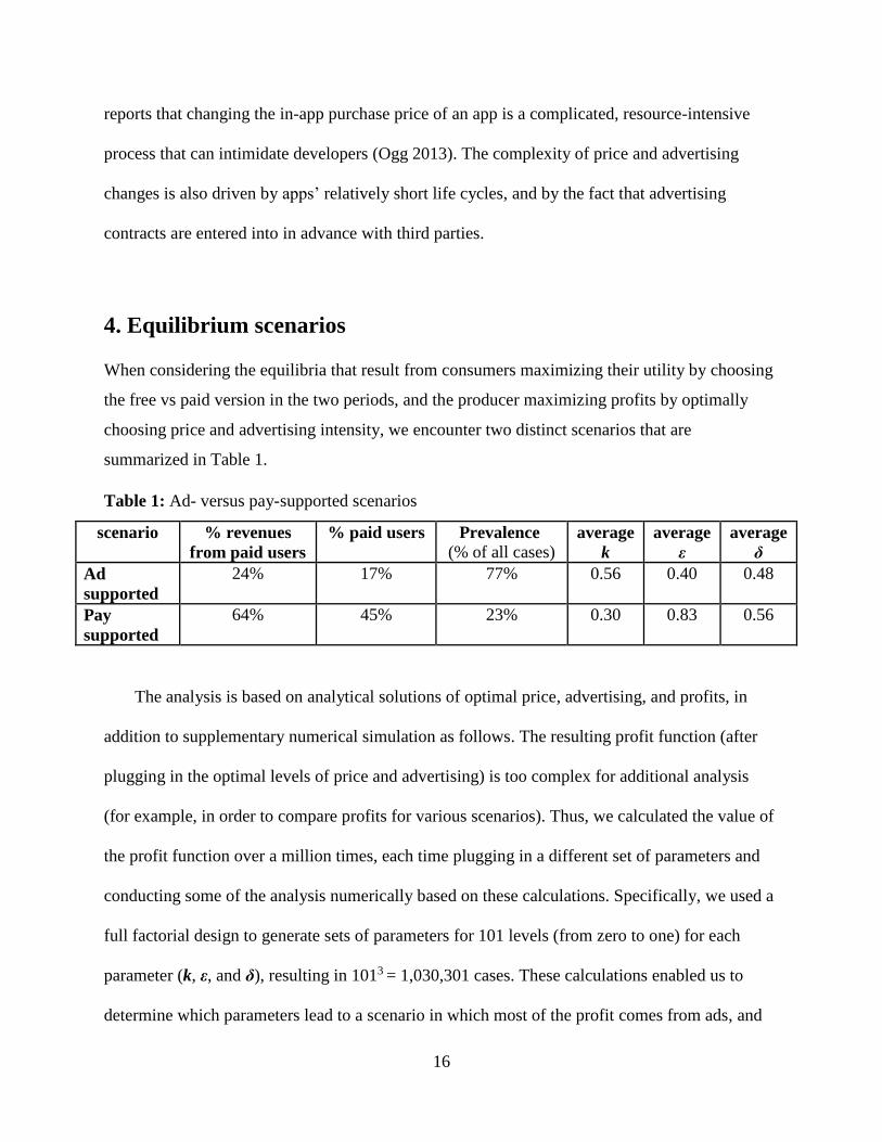
Table 1: Ad- versus pay-supported scenarios

scenario % revenues

from paid users

% paid users Prevalence

(% of all cases) average

k

average

ε

average

δ

Ad

supported

24% 17% 77% 0.56 0.40 0.48

Pay

supported

64% 45% 23% 0.30 0.83 0.56

The analysis is based on analytical solutions of optimal price, advertising, and profits, in

addition to supplementary numerical simulation as follows. The resulting profit function (after

plugging in the optimal levels of price and advertising) is too complex for additional analysis

(for example, in order to compare profits for various scenarios). Thus, we calculated the value of

the profit function over a million times, each time plugging in a different set of parameters and

conducting some of the analysis numerically based on these calculations. Specifically, we used a

full factorial design to generate sets of parameters for 101 levels (from zero to one) for each

parameter (k, ε, and δ), resulting in 1013 = 1,030,301 cases. These calculations enabled us to

determine which parameters lead to a scenario in which most of the profit comes from ads, and

17

those in which most of the profit comes from pay, and then characterize these differing

scenarios.6

The scenarios in Table 1 are divided into two distinct groups: In the first, advertising drives

most of the revenues, while in the second, revenues are driven by the paid version of the app

(second column of Table 1). Note that regardless of whether revenues are driven by advertising

or the paid version, the majority of users of the app download the free version (second column of

Table 1). The two scenarios also differ substantially in their prevalence, as depicted in the third

column of the table, in that the ad-supported scenario constitutes more than three quarters of all

cases. In addition, the scenarios include one additional special case each, to be discussed next.

Observing the average parameter values for each scenario, the ad-supported scenario is

characterized by high advertising effectiveness (k), and low uncertainty (ε). The reason for high k

is obvious: higher advertising effectiveness implies better and more efficient use of resources

devoted to advertising, and, thus ceteris paribus, more revenues will be yielded by this more

efficient tool. With respect to uncertainty, consumers who use the paid version are betting on a

positive outcome of the realization of 𝜇 (+휀 with probability ½). If this happens, they will enjoy

the full benefit of this occurrence, as they do not pay for the app in the second period. Thus

under higher uncertainty, consumers will tend to use the paid version of the app. Lastly, though

the difference is not large, the same reasoning applies to satiation, which implies higher second-

period utility, ergo higher likelihood of choosing the paid version.

6 Note that a) the first three columns contain figures that are outputs of the equilibrium, while the last three contain

the inputs that lead to the equilibrium, and b) the partition into price- vs. ad-supported scenarios is based on the

results, i.e., after calculating the profit, we grouped together the cases that lead to the two rows of the table; and c)

the partitions into cases were continuous, in that they gradually switched from one case to the next. Thus for

example, all cases in which 휀 ≤ 0.44 resulted in the ad-supported scenario. Cases in which 휀 ≥ 0.45 resulted in

gradual increase in the number of pay-supported cases as the parameter k decreased from one to zero.

18

4.1 Ad-supported scenario

This scenario, as well as the pay-supported scenario, is best explained via figures that enable

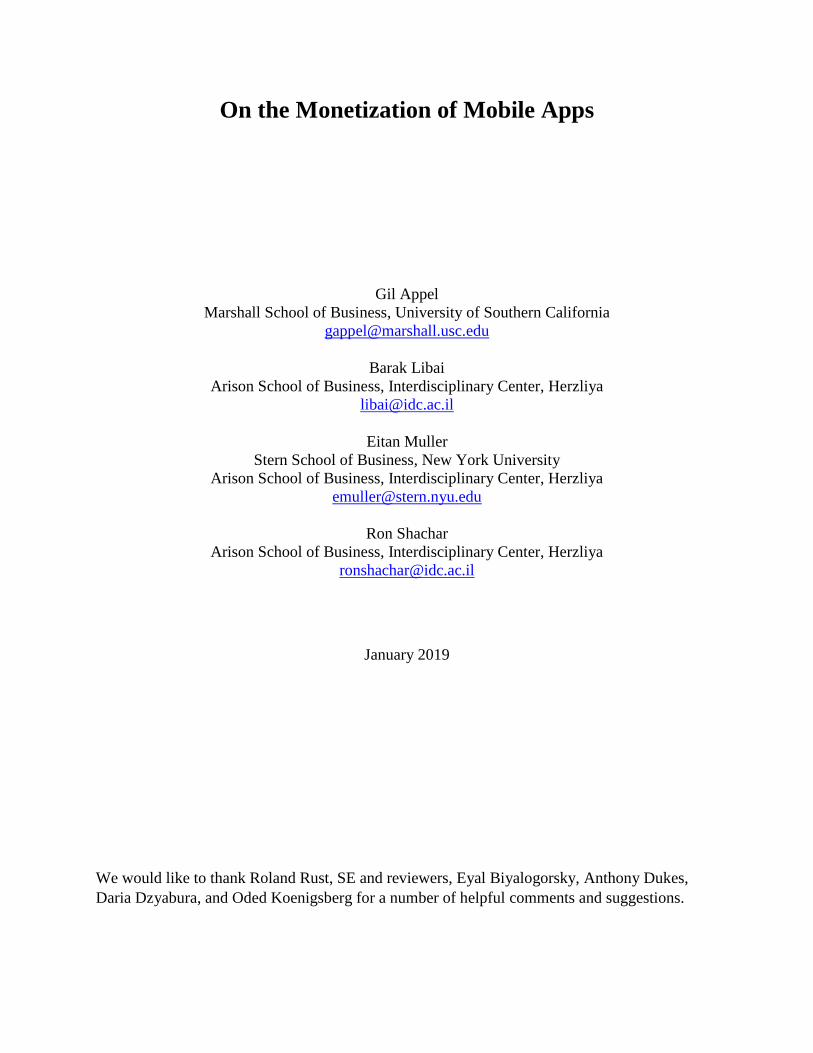
us to derive the demand for the app from its two segments: paid, and free. Figure 1 presents the

relationship between the intrinsic utility 𝛼 and the resulting utility.

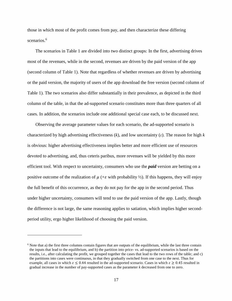
Figure 1: Demand derivation, ad-supported scenario

The red line in Figure 1 represents the users whose intrinsic utility 𝛼 is large enough that it

is optimal for them to download the paid version and stay for two periods. From Equation 2 it is

clear that the user’s utility is 𝛼 − 𝑝 + 𝛼𝛿 where the first term (𝛼 − 𝑝) is her utility in the first

period, while the second term (𝛼𝛿) summarizes her utility in the second period. If her intrinsic

utility 𝛼 is slightly lower, then s/he will download the free version and stay for two periods with

resultant utility of 𝛼(1 − 𝛾) + 𝛼𝛿(1 − 𝛾), as per Equation 3. It is straightforward to check that

19

these two lines intersect when 𝛼 = 𝑝/𝛾(1 + 𝛿). Accordingly, it is easy to check that the two blue

lines intersect when 𝛼 = 휀.

Thus, we have three segments of consumers of differing sizes:

1. For high 𝛼, users download the paid version and stay for two periods. The size of this

segment is 1 − 𝑝/𝛾(1 + 𝛿).

2. For intermediate 𝛼, users download the free version and stay for two periods. The size

of this segment is 𝑝/𝛾(1 + 𝛿) − 휀.

3. For low 𝛼, users download the free version and only those whose realization of 𝜇 is

positive (+휀 with probability ½) will stay for two periods. Their size is thus 휀/2.

When we add these segments, each multiplied by price or advertising as per Equation 4, we

obtain the profits for the app in the two periods as follows:

(5) Π(ad supported scenario) = 𝑝 (1 −𝑝

𝛾(1 + 𝛿) ) + 𝑘𝛾 (

𝑝

𝛾(1 + 𝛿)−휀

2) − 𝛾2

To obtain optimal price and advertising, we differentiate Equation 5 with respect to p and 𝛾

and equate to zero – see Web Appendices A and B for details7.

There is a special case of this scenario in which the intersection point of the paid and free

versions (red and blue lines) is greater than or equal to one (𝑝/𝛾(1 + 𝛿) ≥ 1). Thus in this case

we’re left with only two segments (2 and 3 of the list above). The rest of the analysis follows

through in the same manner, mutatis mutandis, see Web Appendices A and B.

4.2 Pay-supported scenario

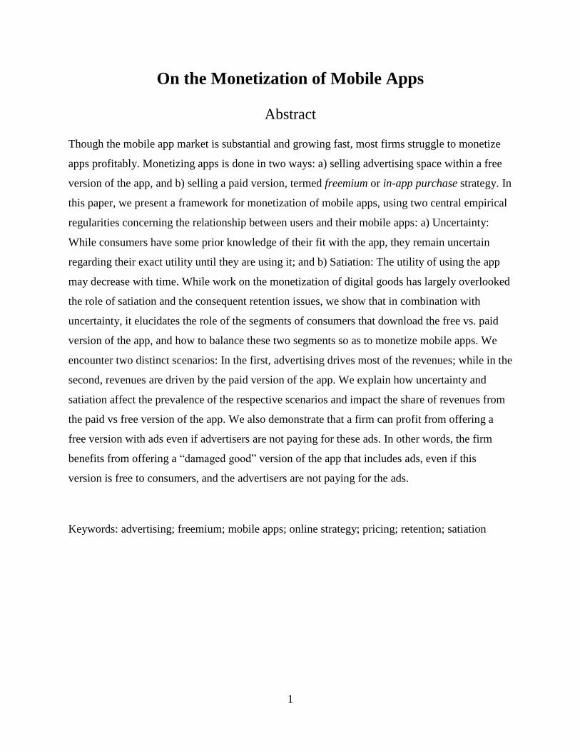
In the same manner as in the ad-supported scenario above, we can construct Figure 2 with its

four segments:

7 It is straightforward to check that for both Equations 5 and 6, the Hessian matrices are negative semidefinite, and

thus second-order conditions for maximization of the profit functions are indeed satisfied.

20

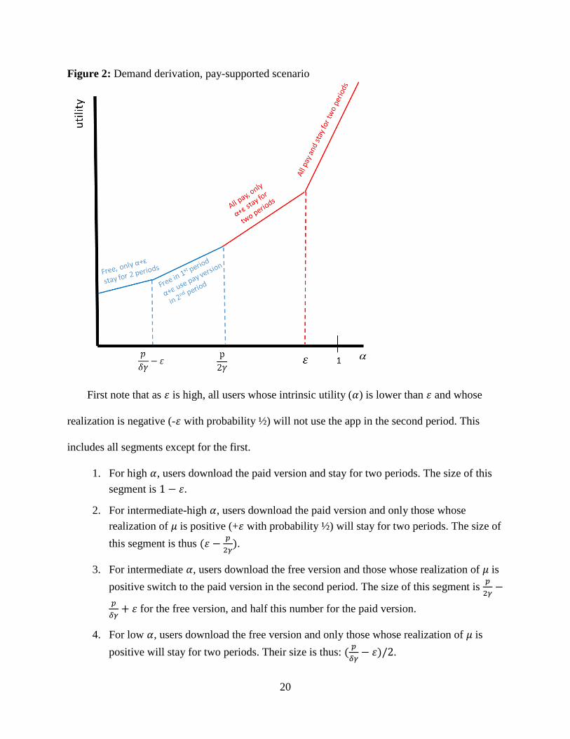
Figure 2: Demand derivation, pay-supported scenario

First note that as 휀 is high, all users whose intrinsic utility (𝛼) is lower than 휀 and whose

realization is negative (-휀 with probability ½) will not use the app in the second period. This

includes all segments except for the first.

1. For high 𝛼, users download the paid version and stay for two periods. The size of this

segment is 1 − 휀.

2. For intermediate-high 𝛼, users download the paid version and only those whose

realization of 𝜇 is positive (+휀 with probability ½) will stay for two periods. The size of

this segment is thus (휀 −𝑝

2𝛾).

3. For intermediate 𝛼, users download the free version and those whose realization of 𝜇 is

positive switch to the paid version in the second period. The size of this segment is 𝑝

2𝛾−

𝑝

𝛿𝛾+ 휀 for the free version, and half this number for the paid version.

4. For low 𝛼, users download the free version and only those whose realization of 𝜇 is

positive will stay for two periods. Their size is thus: (𝑝

𝛿𝛾− 휀)/2.

21

When we add these segments, each multiplied by price or advertising as per Equation 4, we

obtain the profits for the app in the two periods as follows:

(6) Π(pay supported scenario) = 𝑝 (1 −𝑝

2𝛾) +

𝑝

2(𝑝

2𝛾−𝑝

𝛿𝛾+ 휀) + 𝑘𝛾

𝑝

2𝛾+𝑘𝛾

2(𝑝

𝛿𝛾− 휀) − 𝛾2

In order to obtain optimal price and advertising, we differentiate Equation 5 with respect to p

and 𝛾 and equate to zero – see Web Appendices A and B for details.

From Figure 2 it is clear that for Segment 3 to exist (users who download the free version

and whose realization of 𝜇 is positive, and switch to the paid version in the second period),

requires that 𝑝

𝛿𝛾− 휀 ≤

𝑝

2𝛾. There is a special case of this scenario in which the reverse inequality

holds, and thus we’re left with only three segments (1, 2, and 4 of the list above). The rest of the

analysis follows through in the same manner, mutatis mutandis, see Web Appendices A and B.

5. Main results

In this section, we present the main results of our analysis beginning with the effects of the

model’s parameters on the firm’s optimal choices in terms of price and advertising.

5.1 Price and advertising sensitivities

One of the advantages of analytical solutions is that we can derive optimal decision

variables’ sensitivity as a function of the model’s parameters in each of the cases: Ad supported,

and pay supported. The results are given in Web Appendices A and B and presented in Table 2

and Result 1:

22

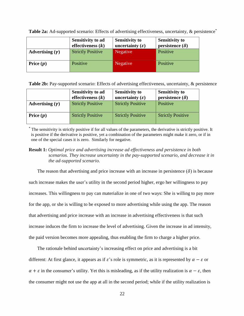
Table 2a: Ad-supported scenario: Effects of advertising effectiveness, uncertainty, & persistence*

Sensitivity to ad

effectiveness (𝒌)

Sensitivity to

uncertainty (𝜺)

Sensitivity to

persistence (𝜹)

Advertising (𝜸) Strictly Positive Negative Positive

Price (𝒑) Positive Negative Positive

Table 2b: Pay-supported scenario: Effects of advertising effectiveness, uncertainty, & persistence

Sensitivity to ad

effectiveness (𝒌)

Sensitivity to

uncertainty (𝜺)

Sensitivity to

persistence (𝜹)

Advertising (𝜸) Strictly Positive Strictly Positive Positive

Price (𝒑) Strictly Positive Strictly Positive Strictly Positive

* The sensitivity is strictly positive if for all values of the parameters, the derivative is strictly positive. It

is positive if the derivative is positive, yet a combination of the parameters might make it zero, or if in

one of the special cases it is zero. Similarly for negative.

Result 1: Optimal price and advertising increase ad effectiveness and persistence in both

scenarios. They increase uncertainty in the pay-supported scenario, and decrease it in

the ad-supported scenario.

The reason that advertising and price increase with an increase in persistence (𝛿) is because

such increase makes the user’s utility in the second period higher, ergo her willingness to pay

increases. This willingness to pay can materialize in one of two ways: She is willing to pay more

for the app, or she is willing to be exposed to more advertising while using the app. The reason

that advertising and price increase with an increase in advertising effectiveness is that such

increase induces the firm to increase the level of advertising. Given the increase in ad intensity,

the paid version becomes more appealing, thus enabling the firm to charge a higher price.

The rationale behind uncertainty’s increasing effect on price and advertising is a bit

different: At first glance, it appears as if 휀’s role is symmetric, as it is represented by 𝛼 − 휀 or

𝛼 + 휀 in the consumer’s utility. Yet this is misleading, as if the utility realization is 𝛼 − 휀, then

the consumer might not use the app at all in the second period; while if the utility realization is

23

𝛼 + 휀, the consumer might either continue to use the free app, or switch to the paid version.

As explained in Figure 1, in the ad-supported scenario, an increase in uncertainty causes

Segment 3 to increase at the expense of the Segment 2, that is, the number of those who stay

increases only if their utility realization is positive at the expense of those who stay regardless of

their utility realization. The net effect is thus negative, causing the firm to lower the costs to

consumers in terms of price and advertising.

As shown in Figure 2, in the pay-supported scenario, uncertainty is high, and all users whose

utility is lower than 휀 and whose realization is negative (-휀 with probability ½) will not use the

app in the second period. This includes three of the four segments. Thus when uncertainty

increases, there is positive asymmetry, as most users would not have used the app in the second

period already. Now that uncertainty has increased, these users’ utility increases in the second

period, causing the firm to increase costs to consumers in terms of advertising and price.

5.2 Share of Revenue shares from free vs paid versions of the app

As we discussed in Section 4.1, there is a special case of an ad-supported scenario in which

there are only two segments, both downloading the free version. Thus, the paid version of the

app is not made available to the users. This is a relatively large case, or about 25% of all cases.

To better understand the reasons behind the firm’s (optimal) decision to offer a free version only,

we note that this sub-scenario is characterized by a very low persistence parameter level (average

𝛿 = 0.33) implying high customer satiation, and relatively high advertising effectiveness

(average k = 0.84). When persistence is low, second-period utility is low, and many consumers

cannot see a justification in paying for the app when it is highly unlikely that they will stay for a

second period. Thus, the company focuses on the free version, wherein more consumers are

more likely to remain, even with low levels of persistence. In this scenario, revenues are

24

generated via ads only, and as adverting effectiveness is high, ads have a good conversion rate,

rendering them more profitable for the firm. This, together with Figure 3b, is summarized by the

following result:

Result 2: When persistence decreases (satiation increases), first, the share of the paid version of

the app decreases, and then with low enough persistence levels (coupled with effective

levels of advertising), the firm offers an ad-supported version of the app only.

Note that persistence in our model is correlated with retention, as it affects second-period

utility, which in turn directly correlates with the decision to stay for the second period. Some

anecdotal evidence supports this relationship: Firstly, in a three-part series of notes about

retention in mobile apps, Balfour (2017) listed four reasons why retention spurs apps’ revenue

growth, the third being that retention improves monetization. The examples given involve four

monetization modes: Advertising, Subscription, Transactional, and Freemium, where in the

latter, he reasons that revenues grow as a result of increased retention, as it increases upgrades

from free to paid versions of apps, which is exactly the model described here.

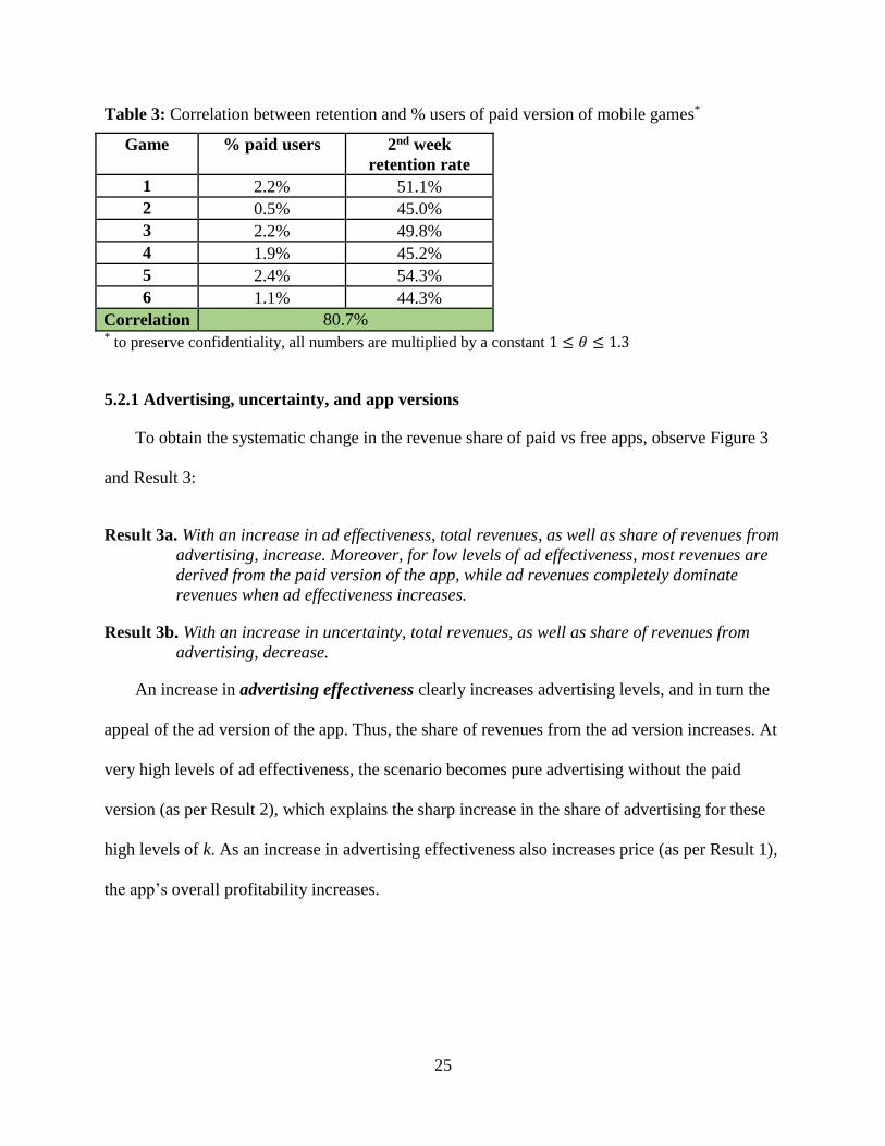
Secondly, we obtained a dataset from an established publisher of multiple casual mobile

game apps for children, several of which reached the Top 100 in the major app stores in recent

years. Our dataset consists of data on the adoption and retention of six apps. Indeed, we observe

a correlation between the percentage of users of the paid versions of the games and retention as

summarized in Table 38.

8 This cannot be construed as an empirical analysis, as we do not have data on control variables that should be

controlled for in an empirical analysis. Thus this is model-free evidence for the correlation.

25

Table 3: Correlation between retention and % users of paid version of mobile games*

Game % paid users 2nd week

retention rate

1 2.2% 51.1%

2 0.5% 45.0%

3 2.2% 49.8%

4 1.9% 45.2%

5 2.4% 54.3%

6 1.1% 44.3%

Correlation 80.7% * to preserve confidentiality, all numbers are multiplied by a constant 1 ≤ 𝜃 ≤ 1.3

5.2.1 Advertising, uncertainty, and app versions

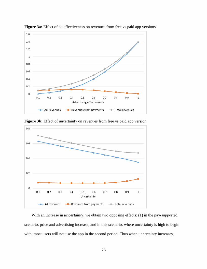
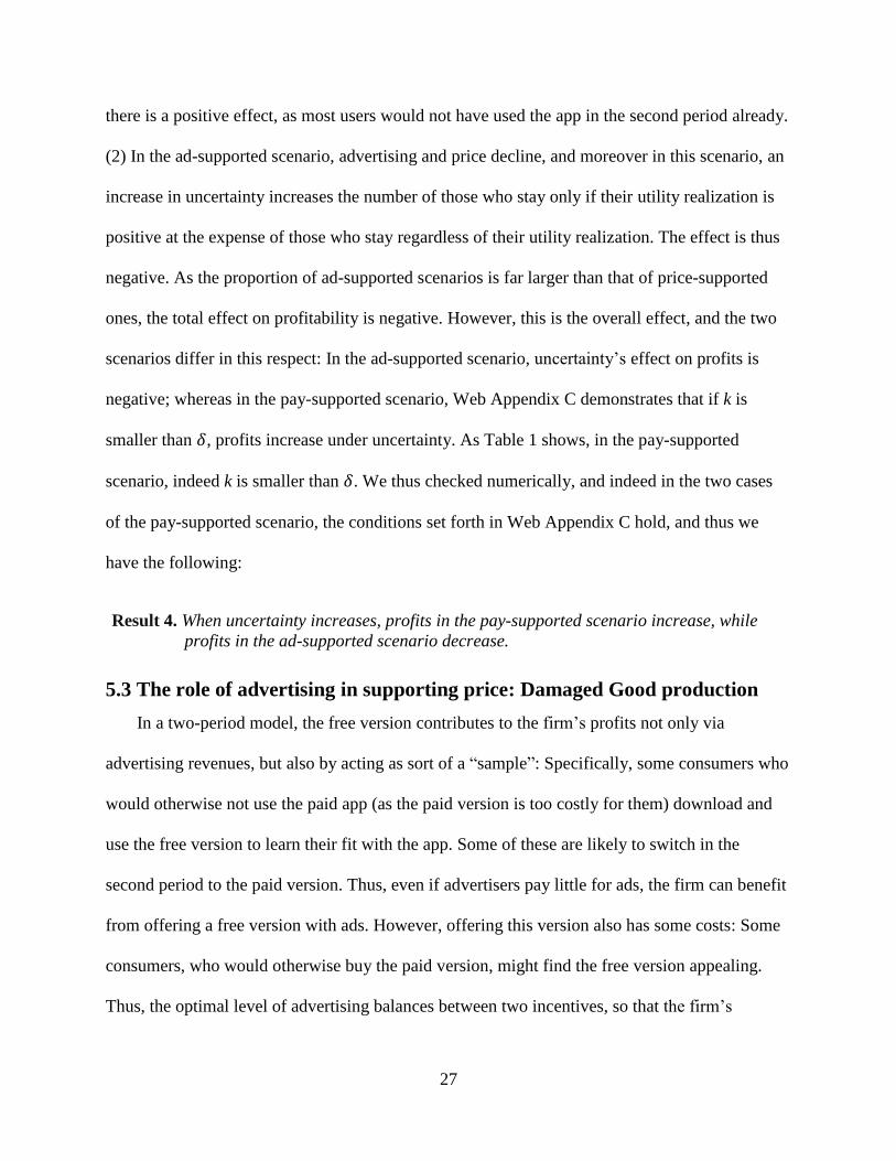
To obtain the systematic change in the revenue share of paid vs free apps, observe Figure 3

and Result 3:

Result 3a. With an increase in ad effectiveness, total revenues, as well as share of revenues from

advertising, increase. Moreover, for low levels of ad effectiveness, most revenues are

derived from the paid version of the app, while ad revenues completely dominate

revenues when ad effectiveness increases.

Result 3b. With an increase in uncertainty, total revenues, as well as share of revenues from

advertising, decrease.

An increase in advertising effectiveness clearly increases advertising levels, and in turn the

appeal of the ad version of the app. Thus, the share of revenues from the ad version increases. At

very high levels of ad effectiveness, the scenario becomes pure advertising without the paid

version (as per Result 2), which explains the sharp increase in the share of advertising for these

high levels of k. As an increase in advertising effectiveness also increases price (as per Result 1),

the app’s overall profitability increases.

26

Figure 3a: Effect of ad effectiveness on revenues from free vs paid app versions

Figure 3b: Effect of uncertainty on revenues from free vs paid app version

With an increase in uncertainty, we obtain two opposing effects: (1) in the pay-supported

scenario, price and advertising increase, and in this scenario, where uncertainty is high to begin

with, most users will not use the app in the second period. Thus when uncertainty increases,

27

there is a positive effect, as most users would not have used the app in the second period already.

(2) In the ad-supported scenario, advertising and price decline, and moreover in this scenario, an

increase in uncertainty increases the number of those who stay only if their utility realization is

positive at the expense of those who stay regardless of their utility realization. The effect is thus

negative. As the proportion of ad-supported scenarios is far larger than that of price-supported

ones, the total effect on profitability is negative. However, this is the overall effect, and the two

scenarios differ in this respect: In the ad-supported scenario, uncertainty’s effect on profits is

negative; whereas in the pay-supported scenario, Web Appendix C demonstrates that if k is

smaller than 𝛿, profits increase under uncertainty. As Table 1 shows, in the pay-supported

scenario, indeed k is smaller than 𝛿. We thus checked numerically, and indeed in the two cases

of the pay-supported scenario, the conditions set forth in Web Appendix C hold, and thus we

have the following:

Result 4. When uncertainty increases, profits in the pay-supported scenario increase, while

profits in the ad-supported scenario decrease.

5.3 The role of advertising in supporting price: Damaged Good production

In a two-period model, the free version contributes to the firm’s profits not only via

advertising revenues, but also by acting as sort of a “sample”: Specifically, some consumers who

would otherwise not use the paid app (as the paid version is too costly for them) download and

use the free version to learn their fit with the app. Some of these are likely to switch in the

second period to the paid version. Thus, even if advertisers pay little for ads, the firm can benefit

from offering a free version with ads. However, offering this version also has some costs: Some

consumers, who would otherwise buy the paid version, might find the free version appealing.

Thus, the optimal level of advertising balances between two incentives, so that the firm’s

28

objective function depends on ad intensity even when 𝑘 = 0. Furthermore, the free version with

ads can yield profits even if advertisers are not paying for these ads.

To examine this idea – that the free version with ads can yield profits even if advertisers are

not paying for these ads – we focused our analysis on all cases in which 𝑘 = 0. Indeed, in all

cases wherein a paid version exists (all except for the subcase of an ad-supported version with no

paid version) we find that the optimal advertising level when 𝑘 = 0 is strictly positive. The firm

has two sources of income: the consumers who downloaded the paid version in the first period;

and the consumers who chose to download the free version in the first period, then switch to the

paid version in the second period. The firm does not realize any revenues from the latter segment

in the first period (as k = 0), but does realize some profits from these consumers in the second

period. This is summarized in the next statement:

Result 5. When advertising effectiveness is zero, the firm still advertises, despite the fact that it

sees no revenues from these ads.

This situation bears similarity to the production of damaged goods (Deneckere and McAfee

1996; Halbheer et al. 2018), where firms deliberately “damage” an entire line of products of their

offering in order to better price discriminate among their customers. An iconic example is IBM

introducing the low-cost Model E laser printer that was identical to the high-cost IBM laser

printer, except for the insertion of a chip that slowed printing from 10 pages per minute to 5

(Deneckere and McAfee 1996). In our case, the app-with-ads is a damaged good, yet the

motivation is not price discrimination: The firm constructs this app knowing that it will not

obtain any direct benefit from it, as it hopes to get some consumers to download it for the sake of

learning its fit to their preferences. The firm makes money only from the paid version of the app,

despite setting an optimal level of advertising for the free version, so that the users will switch to

the paid version where their utility is higher, as this version is free of advertising.

29

6. Discussion

When looking at app markets, managers and consumers may see two broad types of apps.

Some apps are by nature short term, i.e., consumers’ utility may be high early on, yet soon they

can expect to move to the next one. Many games and other hedonic apps fit this description.

Other apps are longer-term in nature: If they fit consumers, they may stick with them for a while.

Business, functional, and other utilitarian apps may better fit this category. What we showed here

is that this distinction may lead to a fundamental difference in optimal management of the

monetization process due to differences in propensity to stay.

We focused on the tension between the main monetization sources: paying consumers versus

paying advertisers. While the tension between the monetization options is recognized as

fundamental to app success (Pozin 2014), in-depth answers as to the drivers of the respective use

of each are lacking. Furthermore, to the best of our knowledge, no previous studies have

analyzed this issue in a customer duration dynamic setting. We show that such a setting, i.e., the

combination of satiation and uncertainty, leads to some important insights on price levels,

advertising intensity, profitability, and profitability sources. We summarize our findings as

follows:

We show that as satiation decreases, prices and advertising intensity increase, and the share

of revenues accruing from the paid version increases. The reason is that an increase in

persistence increases consumers’ willingness to pay, which manifests in one of two ways:

The user is willing to pay more for the app, or he is willing to be exposed to more

advertising while using the app. This pushes some of those who are using the free version

toward the paid version in both periods, or in Period 2. As a result, the share of consumers

who use the paid version increases.

As uncertainty increases, we see two opposing effects: (1) in the pay-supported scenario

where uncertainty is high to begin with, all users whose intrinsic utility is low and whose

realization of uncertainty is negative, will not use the app in the second period. Thus when

30

uncertainty increases, there is a positive effect, as most users would not have used the app

in the second period in any case (with the lower uncertainty). Thus in the pay-supported

scenario, profits increase under uncertainty. (2) In the ad-supported scenario, an increase in

uncertainty increases the number of those who stay only if their utility realization is

positive, at the expense of those who stay regardless of their utility realization. The effect is

thus negative. As the proportion of the ad-supported scenarios is far larger than the pay-

supported ones, the total effect on profitability is negative.

We demonstrate that a firm can profit from offering a free app version with ads even if

advertisers are not paying for those ads. In other words, the firm benefits from offering a

version of the app that includes ads even if the consumers are not paying for the app and

the advertisers are not paying for the ads. The logic behind offering this “damaged good” is

that in a dynamic setting, the free version acts as a sort of “sample” that enables consumers

to learn their fit with the app. The firm would rather add ads to this version (even if they’re

not paid for) in order to retain the consumers who have high valuation of the app away

from the “sample” and buying the paid version.

6.1 Managerial implications

The question of how to treat apps via the two main mechanisms of free (advertising) and

paid (premium version, or in-app purchase) versions, is key to app management, in particular

given many apps’ low profitability. Thus, managers are encouraged to study the profitability

outcome of the various options and understand their sources (Nathanson 2016). Our work carries

a number of implications that contribute to this discussion.

Setting realistic expectations

How many paid vs free downloads should app makers expect? To what extent does the

percentage of each signal an app’s success? A straightforward way to look at composition of

paid versus unpaid apps uses a simple segmentation scheme under which there are two kinds of

users: Those who see limited value in the app, and thus will not be willing to pay; and those who

see greater value and are willing to pay. Because the app maker may find it hard to assess the

31

nature of newcomers, they will offer a free version up front, and charge some price for a

minority that desires higher utility (Nathanson 2016).

While this approach helps to portray a simple-to-understand picture of the market, our

analysis demonstrates that the respective shares of paid and free apps are in fact a function of a

complex process. Uncertainty, satiation, and the marketing mix elements of price and advertising

effectiveness combine to determine the market outcome. The advantage of a formal analytical

approach lies in the ability to portray the dynamics that shape the utility function, and understand

the impact of the various factors that create the emerging dynamics. This view has a direct effect

when forming expectations of the profitability created by apps. For example, an ongoing debate

among investors and venture capitalists surrounds the viability of freemium business models

(Maltz 2012). Understanding the complexity of the situation will enable entrepreneurs and

investors alike to form more educated expectations based on the app-related models; identify

strengths and weaknesses; and formulate business strategies that take into account the

endogenous ways in which the shares of paid versus free versions could be forecasted and

realized.

Realistic expectations should also be formed regarding the effectiveness of marketing mix

elements in the app monetization environment. As Result 5 suggests, advertising’s effectiveness

should be considered in a wider perspective that takes into account its overall effect on

profitability in the free versus paid app monetization environment.

Carefully balancing investments in paid vs. free app versions

Result 2 demonstrates the delicate balance that must be struck between the free vs paid app

versions in terms of investment in satiation reduction, price promotion, and advertising levels.

Any change in one of these variables in turn alters the composition of the segments that

32

download the free vs paid app version. Furthermore, this composition has a direct effect on the

app’s profitability, as Result 3 demonstrates. Moreover, the composition has an effect on

retention, as paid users have higher retention rates (see Result 2 and Table 3).

An interesting issue is the effect of uncertainty: Note that the majority of users download

and use free app versions, where revenues and retention, and thus lifetime value, are lower. Thus

firms are trying to contrive ways to move users from free to paid app versions. Having said this,

the free version plays a major role in the face of uncertainty: It is used by consumers as a

sampling device, so as to better learn the app’s idiosyncratic value to them. Later on they can

decide to continue using the free version, or switch to the paid one, or else drop the app from

further consideration. It is this role of sampling that renders uncertainty profitable under the pay-

supported scenario – higher uncertainty induces users to try the free version and then switch to

the paid version of the app, as in this scenario, the cost of advertising to the consumer is high

(relative to price).

Investing in satiation reduction

Our results highlight in particular satiation’s role, and how persistence with the app affects

profitability. The contribution of customer duration to app profitability and survival is

increasingly acknowledged by industry observers (Jacobson 2018). App makers are encouraged

to consider user retention at the expense of acquisition, and formulate ways to deliver more value

to users and be in touch with them so they will stay (Perro 2018). These efforts are particularly

notable for mobile apps given the difficulty in retaining adopters of free products (Datta,

Foubert, and Van Heerde 2015).

Given the expected effect of satiation on app use duration, as is also cited here, app creators

can draw from the emerging behavioral literature on satiation. For example, to decrease satiation,

33

managers may want to encourage users to change their consumption rates (Galak, Kruger, and

Loewenstein 2013), or to think of future variety (Sevilla, Zhang, and Kahn 2016). Apps may

want to manage the similarity of new experiences the users get (Lasaleta and Redden 2018), or

limit the times for which the products are available (Sevilla and Redden 2014).

Yet the road from persistence to retention is not always linear and straightforward. As Result

2 shows, satiation is correlated with the share of users who download the free version of the app,

which in turn affects both profitability from current users as well as retention, as free users have

lower retention rates. What we see is the indirect way in which satiation affects the marketing

mix. The classic effect of retention on profit is considered to be direct, through customer lifetime

value (Ascarza et al. 2018). Persistence will certainly have an effect in this direction. Yet as we

see in Result 1, persistence also has a positive impact on advertising levels and on the price to be

charged for the paid version. App creators should thus deeply examine ways to decrease

satiation, and consider carefully the positive consequences of these efforts.

6.2 Limitations

Our attempt to capture a complex market situation with a relatively parsimonious model

clearly has a number of limitations. One issue is the lack of explicit modeling of competitive

activity, which takes into account alternative space, time, and competitive apps. The added

complexity thereof is beyond our scope here. It should also be mentioned that it is not trivial to

model explicit competition, due to the complex meaning of what constitutes a “competitor” in

this market. Many free products compete in a general sense for users’ attention and time, and not

necessarily with products to which they are very similar. However, there may be specific

categories in which clear, direct competitors emerge.

We examined a specific freemium model in which the product’s premium version had no

34

advertising. There are more complex free business models in which, for example, users purchase

in-app add-ons that change the product’s utility in various ways. Modeling each of these

scenarios would add complexity that we feel is unneeded at this stage, yet can of course be done

in future explorations. In the same vein, we assumed a fixed price for the paid version. This

assumption is supported by market observations and interviews with managers, which suggest

that given the short time periods, the paid version price is largely fixed. Changing this

assumption adds significant complexity, yet can be an interesting avenue for future research.

Finally, further analysis might wish to examine peer effects, which are absent from our

analysis. When a customer leaves, it may affect not only the firm’s ability to acquire other

customers via word of mouth, but may also lead to the churn of other current customers (Nitzan

and Libai 2011). This may further emphasize the importance of efforts to decrease satiation, and

increase customer utility in general. Furthermore, existing paying customers may affect the other

customers’ utility by creating within-customer contagion processes (Bapna and Umyarov 2015).

In this sense, there is still a way to go toward better understanding of the complex process in

which profitability is created when monetizing free versus paid apps.

35

References

Ackerberg, D. 2003. Advertising, learning, and consumer choice in experience good markets: An

empirical examination. Internat. Econom. Rev. 44(3), 1007-1040.

App Annie. 2016. New from App Annie: Competitive app retention data. June 16.

App Brain. 2018. Free vs. paid Android apps. December 24.

AppsFlyer. 2017. The state of app engagement. February.

Arora, S., F. T. Hofstede, and V. Mahajan. 2017. The implications of offering free versions for

the performance of paid mobile apps. J. of Marketing 81(3), 62-78.

Ascarza, E; S. Neslin, O. Netzer, Z. Anderson, P. Fader, S. Gupta, B. Hardie, A. Lemmens, B.

Libai, D. Neal, F. Provost, and R. Schrift. 2018. In pursuit of enhanced customer retention

management. Customer Need and Solutions, 5(1-2), 65-81.

Assmus, G., J. Farley, and D. Lehmann. 1984. How advertising affects sales: Meta-analysis of

econometric results. J. Marketing Res. 21(1), 65-74.

Balfour, B. 2017. Growth loops are the new funnels. Reforge.

Babu, S. 2018. Are you mobile ready? The state of mobile conversions report will tell you.

Martech Advisor, January 10.

Bapna, R. and A. Umyarov. 2015. Do your online friends make you pay? A randomized field

experiment on peer influence in online social networks. Management Sci., 61(8), 1902-

1920.

Biyalogorsky, E. and O. Koenigsberg. 2014. The design and introduction of product lines when

consumer valuations are uncertain. Production and Operations Management, 23(9), 1539-

1548.

Cheney, S. and E. Thompson. 2018. The 2017-2022 app economy forecast: 6 billion devices,

$157 billion in spend and more. App Annie.

Datta, H., B. Foubert, H. J. Van Heerde. 2015. The challenge of retaining customers acquired

with free trials. J. Marketing Res. 52(2), 217-234.

Deneckere, R.J. and Preston McAfee, R., 1996. Damaged goods. Journal of Economics &

Management Strategy, 5(2), 149-174.

Deng, Y., A. Lambrecht, and Y. Liu. 2018. Spillover effects and freemium strategy in mobile

app market. SSRN.

36

Erdem, T., J. Swait, S. Broniarczyk, D. Chakravarti, J. Kapferer, M. Keane, J. Roberts, J. B.

Steenkamp, and F. Zettelmeyer. 1999. Brand equity, consumer learning, and choice.

Marketing Lett. 10(3), 301-318.

Galak, J., J. Kruger, and G. Loewenstein. 2013. Slow down! Insensitivity to rate of consumption

leads to avoidable satiation. J of Cons. Research 39(5), 993-1009.

Galak, J. and J. P. Redden. 2018. The properties and antecedents of hedonic decline. Ann Rev

Psych. 69, 1-25.

Gu, X., P. K. Kannan, and L. Ma. 2018. Selling the premium in freemium. J of Marketing, 82(6),

10-27.

Foubert, B. and E. Gijsbrechts. 2016. Try it, you’ll like it—or will you? The perils of early free-

trial promotions for high-tech service adoption. Marketing Sci. 35(5), 810-826.

Godes, D., E. Ofek, and M. Sarvary. 2009. Content vs. advertising: The impact of competition on

media firm strategy. Marketing Sci. 28(1), 20-35.

Goldstein, D. G., S. Suri, R. P. McAfee, M. Ekstrand-Abueg, and F. Diaz. 2014. The economic

and cognitive costs of annoying display advertisements. J. Marketing Res. 51(6), 742-752.

Halbheer, D., D. L. Gärtner, E. Gerstner, and O. Koenigsberg. 2018. Optimizing service failure

and damage control. Internat. J. Res Marketing, 35(1), 100-115.

Halbheer, D., F. Stahl, O. Koenigsberg, and D. R. Lehmann. 2014. Choosing a digital content

strategy: How much should be free? Internat. J. Res. Marketing 31(2), 192-206.

Han, S. P., S. Park, and W. Oh. 2016. Mobile app analytics: A multiple discrete-continuous

choice framework. MIS Quarterly 40(4), 983-1008.

Hong, Y. and P. A. Pavlou. 2014. Product fit uncertainty in online markets: Nature, effects, and

antecedents. Inform. Systems Res., 25(2), 328-344.

Hui, S. K. (2017). Understanding repeat playing behavior in casual games using a Bayesian data

augmentation approach. Quant. Marketing and Econo. 15(1), 29-55.

Hsu, C-L. and J. C-C. Lin 2016. Effect of perceived value and social influences on mobile app

stickiness and in-app purchase intention. Tech. Forecasting Soc. Change 108, 42-53.

Jacobson, B. 2018. How mobile app retention is evolving. PostFunnel, July 19.

Iyengar, R., A. Ansari, and S. Gupta. 2007. A model of consumer learning for service quality and

usage. J. Marketing Res. 44(3), 529-544.

Kannan, P. K. 2013. Designing and pricing digital content products and services: A research

review. Rev. Marketing Res. 10, 97-114.

37

Kannan, P.K., and H. A. Li. 2017. Digital marketing: A framework, review, and research agenda.

Internat. J. Res. Marketing 34(1), 22-45.

Klotzbach, C. 2016. Enter the matrix: App retention and engagement. Flurry Insights, May 12.

Lagace, M. 2018. Mobile gaming has an advertising problem that needs to be addressed.

AndroidCentral, Feb 21.

Lambrecht, A., A. Goldfarb, A. Bonatti, A. Ghose, D. Goldstein, R. Lewis, A. Rao, N. Sahni,

and S. Yao. 2014. How do firms make money selling digital goods online? Marketing Lett.

25(3), 331-341.

Lambrecht, A. and K. Misra. 2016. Fee, or free? When should firms charge for online content?

Management Sci. 63(4), 1150-1165.

Lasaleta, J.D. and Redden, J.P. 2018. When Promoting Similarity Slows Satiation: The

Relationship of Variety, Categorization, Similarity, and Satiation. J. of Marketing

Res. 55(3), 446-457.

Lee, C., V. Kumar, and S. Gupta. 2017. Designing freemium: Balancing growth and

monetization strategies. SSRN.

Li, H. A., S. Jain, and P. K. Kannan. 2019. Optimal design of content samples for digital

products and services. J. Marketing Res. forthcoming.

Libai, B., E. Muller, and R. Peres. 2009. The diffusion of services. J. Marketing Res. 46(2), 163-

175.

Maltz, J. 2012. Should your startup go freemium? TechCrunch.

Moorthy, K.S., 1984. Market segmentation, self-selection, and product line design. Marketing

Sci. 3(4), 288-307.

Moorthy, K.S. and Png, I.P., 1992. Market segmentation, cannibalization, and the timing of

product introductions. Management Sci. 38(3), 345-359.

Morvinski, C., O. Amir, and E. Muller. 2017. “Ten million readers can’t be wrong!” Or can

they? On the role of information about adoption stock in new product trial. Marketing Sci.

36(2), 290-300.

Musalem, A. and Y. V. Joshi. 2009. How much should you invest in each customer relationship?

A competitive strategic approach. Marketing Sci. 28(3), 555-565.

Natanson, E. 2016. “Ebony and ivory”: The blended in-app purchase and advertising model.

Forbes, July 7.

Needleman, S. E. 2016. How mobile games rake in billions. Wall Street Journal, July 28.

38

Niculescu, M. F. and D. J. Wu. 2014. Economics of free under perpetual licensing: Implications

for the software industry. Informat. Systems Res. 25(1), 173-199.

Ogg, E. 2013. Why even the best iOS app developers struggle to set the right price. Gigaop, June

19.

Pauwels, K. and A. Weiss. 2008. Moving from free to fee: How online firms market to change

their business model successfully. J. Marketing 72(3), 14-31.

Perro, J. (2018). Mobile apps: What’s a good retention rate? Localytics, March 22.

Pindyck, R.S., 1982. Adjustment costs, uncertainty, and the behavior of the firm. The American

Economic Review, 72(3), 415-427.

Pozin, I. 2014. How to monetize your app: Banner ads vs native ads vs in-app purchases. Forbes,

December 31.

Prasad, A., V. Mahajan, and B. Bronnenberg. 2003. Advertising versus pay-per-view in

electronic media. Internat. J. Res. Marketing 20(1), 13-30.

Schulze, C., L. Schöler, and B. Skiera. 2014. Not all fun and games: Viral marketing for

utilitarian products. J of Marketing 78(1), 1-19.

Sevilla, J. and J. P. Redden. 2014. Limited availability reduces the rate of satiation. J. Marketing

Res, 51(2), 205-217.

Sevilla, J., J. Zhang, and B. E. Kahn. 2016. Anticipation of future variety reduces satiation from

current experiences. J. Marketing Res. 53(6), 954-968.

Shin, J. and K. Sudhir. 2012. When to “fire” customers: Customer cost-based pricing.

Management Sci. 58(5), 932-947.

Statista. 2018. Number of apps available in leading app stores as of 1st quarter 2018.

Subramanian, U., J. S. Raju, and J. Zhang. 2013. The strategic value of high-cost customers.

Management Sci. 60(2), 494-507.

Tåg, J. 2009. Paying to remove advertisements. Informat. Economics Policy 21(4), 245-252.

Vakratsas, D. and Ambler, T., 1999. How advertising works: what do we really know? The

Journal of Marketing, 63(1), 26-43.

Voss, G. B., A. Godfrey, and K. Seiders. 2010. How complementarity and substitution alter the

customer satisfaction–repurchase link. J. Marketing, 74(6), 111-127.

Wijman, T. 2018. Mobile revenues account for more than 50% of the global games market as it

reaches $137.9 billion in 2018. Newzoo, April 30.

Wilbur, K. C. 2008. A two-sided, empirical model of television advertising and viewing

markets. Marketing Sci. 27(3), 356-378.

39

Web Appendices

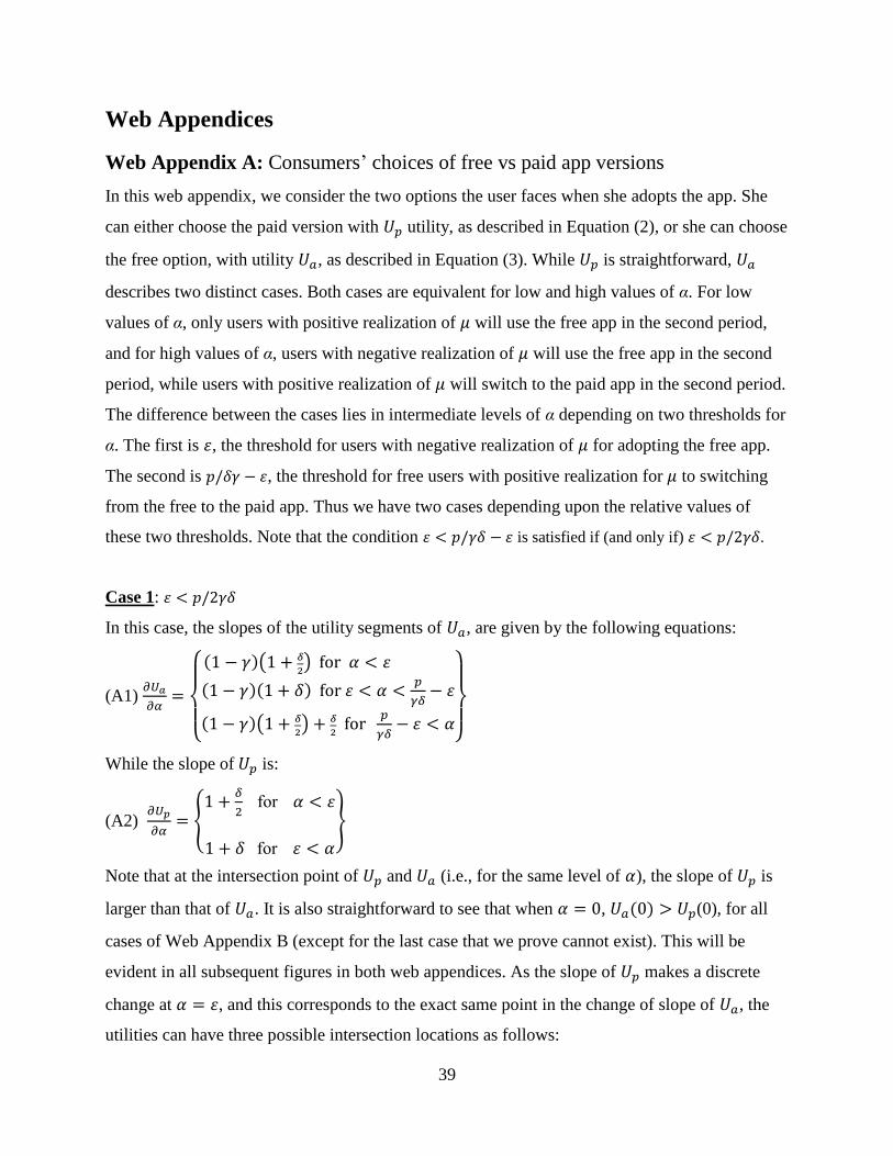
Web Appendix A: Consumers’ choices of free vs paid app versions

In this web appendix, we consider the two options the user faces when she adopts the app. She

can either choose the paid version with 𝑈𝑝 utility, as described in Equation (2), or she can choose

the free option, with utility 𝑈𝑎, as described in Equation (3). While 𝑈𝑝 is straightforward, 𝑈𝑎

describes two distinct cases. Both cases are equivalent for low and high values of α. For low

values of α, only users with positive realization of 𝜇 will use the free app in the second period,

and for high values of α, users with negative realization of 𝜇 will use the free app in the second

period, while users with positive realization of 𝜇 will switch to the paid app in the second period.

The difference between the cases lies in intermediate levels of α depending on two thresholds for

α. The first is 휀, the threshold for users with negative realization of 𝜇 for adopting the free app.

The second is 𝑝/𝛿𝛾 − 휀, the threshold for free users with positive realization for 𝜇 to switching

from the free to the paid app. Thus we have two cases depending upon the relative values of

these two thresholds. Note that the condition 휀 < 𝑝/𝛾𝛿 − 휀 is satisfied if (and only if) 휀 < 𝑝/2𝛾𝛿.

Case 1: 휀 < 𝑝/2𝛾𝛿

In this case, the slopes of the utility segments of 𝑈𝑎, are given by the following equations:

(A1) 𝜕𝑈𝑎

𝜕𝛼=

{

(1 − 𝛾)(1 +

𝛿

2) for 𝛼 < 휀

(1 − 𝛾)(1 + 𝛿) for 휀 < 𝛼 <𝑝

𝛾𝛿− 휀

(1 − 𝛾)(1 + 𝛿

2) + 𝛿

2 for

𝑝

𝛾𝛿− 휀 < 𝛼

}

While the slope of 𝑈𝑝 is:

(A2) 𝜕𝑈𝑝

𝜕𝛼= {

1 +𝛿

2 for 𝛼 < 휀

1 + 𝛿 for 휀 < 𝛼

}

Note that at the intersection point of 𝑈𝑝 and 𝑈𝑎 (i.e., for the same level of 𝛼), the slope of 𝑈𝑝 is

larger than that of 𝑈𝑎. It is also straightforward to see that when 𝛼 = 0, 𝑈𝑎(0) > 𝑈𝑝(0), for all

cases of Web Appendix B (except for the last case that we prove cannot exist). This will be

evident in all subsequent figures in both web appendices. As the slope of 𝑈𝑝 makes a discrete

change at 𝛼 = 휀, and this corresponds to the exact same point in the change of slope of 𝑈𝑎, the

utilities can have three possible intersection locations as follows:

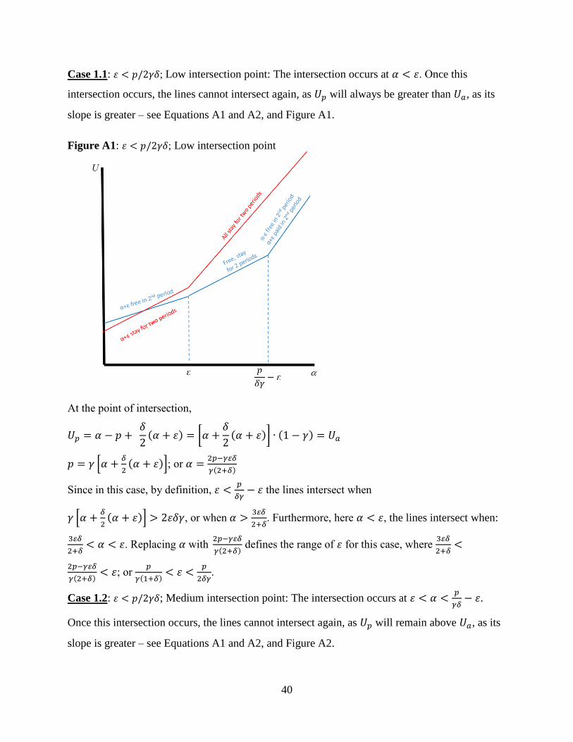
40

Case 1.1: 휀 < 𝑝/2𝛾𝛿; Low intersection point: The intersection occurs at 𝛼 < 휀. Once this

intersection occurs, the lines cannot intersect again, as 𝑈𝑝 will always be greater than 𝑈𝑎, as its

slope is greater – see Equations A1 and A2, and Figure A1.

Figure A1: 휀 < 𝑝/2𝛾𝛿; Low intersection point

At the point of intersection,

𝑈𝑝 = 𝛼 − 𝑝 + 𝛿

2(𝛼 + 휀) = [𝛼 +

𝛿

2(𝛼 + 휀)] ∙ (1 − 𝛾) = 𝑈𝑎

𝑝 = 𝛾 [𝛼 +𝛿

2(𝛼 + 휀)]; or 𝛼 =

2𝑝−𝛾 𝛿

𝛾(2+𝛿)

Since in this case, by definition, 휀 <𝑝

𝛿𝛾− 휀 the lines intersect when

𝛾 [𝛼 +𝛿

2(𝛼 + 휀)] > 2휀𝛿𝛾, or when 𝛼 >

3 𝛿

2+𝛿. Furthermore, here 𝛼 < 휀, the lines intersect when:

3 𝛿

2+𝛿< 𝛼 < 휀. Replacing 𝛼 with

2𝑝−𝛾 𝛿

𝛾(2+𝛿) defines the range of 휀 for this case, where

3 𝛿

2+𝛿<

2𝑝−𝛾 𝛿

𝛾(2+𝛿)< 휀; or

𝑝

𝛾(1+𝛿)< 휀 <

𝑝

2𝛿𝛾.

Case 1.2: 휀 < 𝑝/2𝛾𝛿; Medium intersection point: The intersection occurs at 휀 < 𝛼 <𝑝

𝛾𝛿− 휀.

Once this intersection occurs, the lines cannot intersect again, as 𝑈𝑝 will remain above 𝑈𝑎, as its

slope is greater – see Equations A1 and A2, and Figure A2.

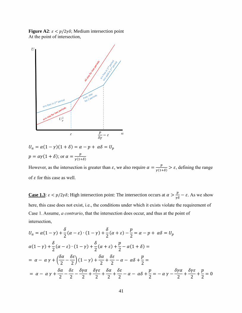
41

Figure A2: 휀 < 𝑝/2𝛾𝛿; Medium intersection point

At the point of intersection,

𝑈𝑎 = 𝛼(1 − 𝛾)(1 + 𝛿) = 𝛼 − 𝑝 + 𝛼𝛿 = 𝑈𝑝

𝑝 = 𝛼𝛾(1 + 𝛿); or 𝛼 =𝑝

𝛾(1+𝛿)

However, as the intersection is greater than 휀, we also require 𝛼 =𝑝

𝛾(1+𝛿)> 휀, defining the range

of 휀 for this case as well.

Case 1.3: 휀 < 𝑝/2𝛾𝛿; High intersection point: The intersection occurs at 𝛼 >𝑝

𝛾𝛿− 휀. As we show

here, this case does not exist, i.e., the conditions under which it exists violate the requirement of

Case 1. Assume, a contrario, that the intersection does occur, and thus at the point of

intersection,

𝑈𝑎 = 𝛼(1 − 𝛾) +𝛿

2(𝛼 − 휀) ∙ (1 − 𝛾) +

𝛿

2(𝛼 + 휀) −

𝑝

2= 𝛼 − 𝑝 + 𝛼𝛿 = 𝑈𝑝

𝛼(1 − 𝛾) +𝛿

2(𝛼 − 휀) ∙ (1 − 𝛾) +

𝛿

2(𝛼 + 휀) +

𝑝

2− 𝛼(1 + 𝛿) =

= 𝛼 − 𝛼 𝛾 + (𝛿𝛼

2−𝛿휀

2) (1 − 𝛾) +

𝛿𝛼

2+𝛿휀

2− 𝛼 − 𝛼𝛿 +

𝑝

2=

= 𝛼 − 𝛼 𝛾 +𝛿𝛼

2−𝛿휀

2−𝛿𝛾𝛼

2+𝛿𝛾휀

2+𝛿𝛼

2+𝛿휀

2− 𝛼 − 𝛼𝛿 +

𝑝

2= − 𝛼 𝛾 −

𝛿𝛾𝛼

2+𝛿𝛾휀

2+𝑝

2= 0

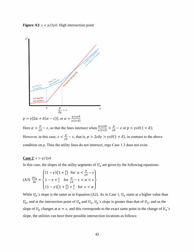
42

Figure A3: 휀 < 𝑝/2𝛾𝛿; High intersection point

𝑝 = 𝛾[2𝛼 + 𝛿(𝛼 − 휀)]; or 𝛼 =𝑝+𝛾 𝛿

𝛾(2+𝛿)

Here 𝛼 >𝑝

𝛾𝛿− 휀, so that the lines intersect when

𝑝+𝛾 𝛿

𝛾(2+𝛿)>

𝑝

𝛾𝛿− 휀 or 𝑝 < 𝛾휀𝛿(1 + 𝛿);

However, in this case, 휀 <𝑝

𝛾𝛿− 휀, that is, 𝑝 > 2휀𝛿𝛾 > 𝛾휀𝛿(1 + 𝛿), in contrast to the above

condition on p. Thus the utility lines do not intersect, ergo Case 1.3 does not exist.

Case 2: 휀 > 𝑝/2𝛾𝛿

In this case, the slopes of the utility segments of 𝑈𝑎 are given by the following equations:

(A3) 𝜕𝑈𝑎

𝜕𝛼=

{

(1 − 𝛾)(1 +

𝛿

2) for 𝛼 <

𝑝

𝛾𝛿− 휀

1 − 𝛾 + 𝛿

2 for

𝑝

𝛾𝛿− 휀 < 𝛼 < 휀

(1 − 𝛾)(1 + 𝛿

2) + 𝛿

2 for 휀 < 𝛼}

While 𝑈𝑝’s slope is the same as in Equation (A2). As in Case 1, 𝑈𝑎 starts at a higher value than

𝑈𝑝, and at the intersection point of 𝑈𝑝 and 𝑈𝑎, 𝑈𝑝’s slope is greater than that of 𝑈𝑎, and as the

slope of 𝑈𝑝 changes at 𝛼 = 휀, and this corresponds to the exact same point in the change of 𝑈𝑎’s

slope, the utilities can have three possible intersection locations as follows:

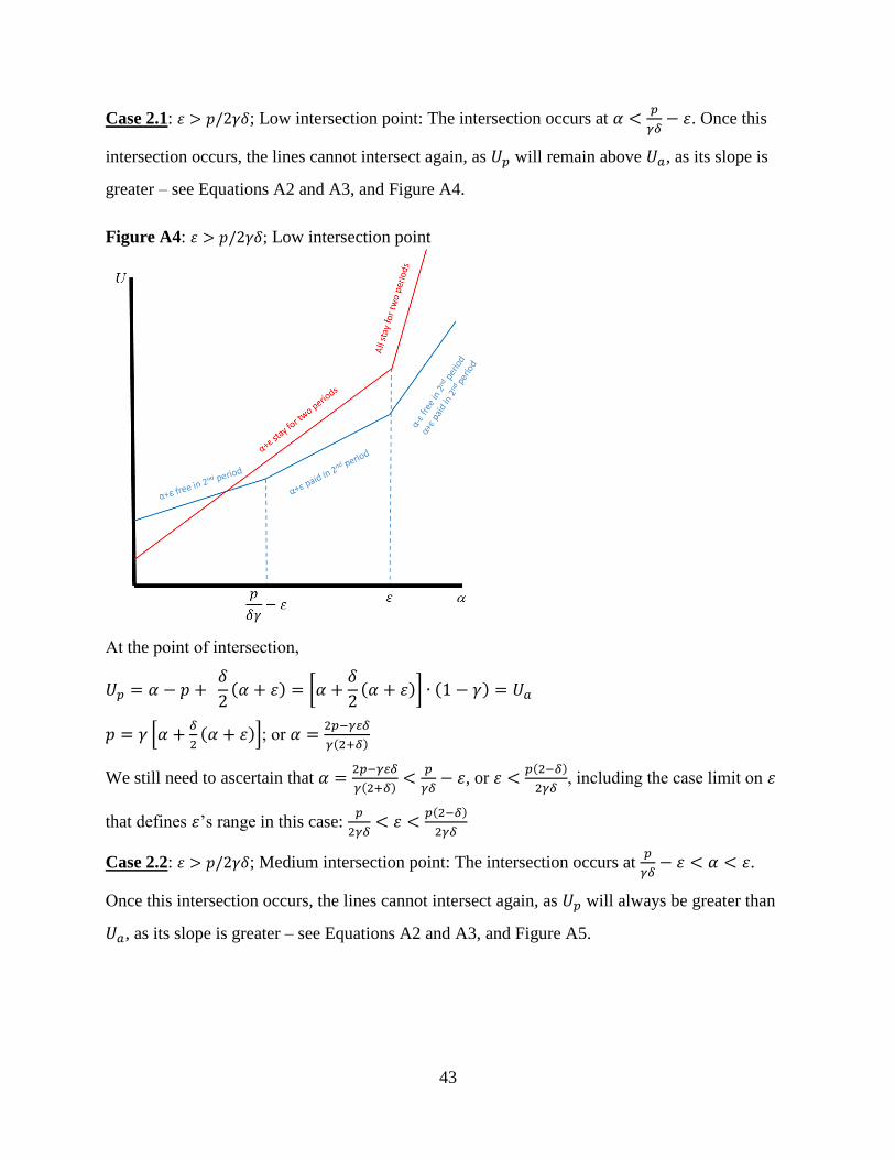
43

Case 2.1: 휀 > 𝑝/2𝛾𝛿; Low intersection point: The intersection occurs at 𝛼 <𝑝

𝛾𝛿− 휀. Once this

intersection occurs, the lines cannot intersect again, as 𝑈𝑝 will remain above 𝑈𝑎, as its slope is

greater – see Equations A2 and A3, and Figure A4.

Figure A4: 휀 > 𝑝/2𝛾𝛿; Low intersection point

At the point of intersection,

𝑈𝑝 = 𝛼 − 𝑝 + 𝛿

2(𝛼 + 휀) = [𝛼 +

𝛿

2(𝛼 + 휀)] ∙ (1 − 𝛾) = 𝑈𝑎

𝑝 = 𝛾 [𝛼 +𝛿

2(𝛼 + 휀)]; or 𝛼 =

2𝑝−𝛾 𝛿

𝛾(2+𝛿)

We still need to ascertain that 𝛼 =2𝑝−𝛾 𝛿

𝛾(2+𝛿)<

𝑝

𝛾𝛿− 휀, or 휀 <

𝑝(2−𝛿)

2𝛾𝛿, including the case limit on 휀

that defines 휀’s range in this case: 𝑝

2𝛾𝛿< 휀 <

𝑝(2−𝛿)

2𝛾𝛿

Case 2.2: 휀 > 𝑝/2𝛾𝛿; Medium intersection point: The intersection occurs at 𝑝

𝛾𝛿− 휀 < 𝛼 < 휀.

Once this intersection occurs, the lines cannot intersect again, as 𝑈𝑝 will always be greater than

𝑈𝑎, as its slope is greater – see Equations A2 and A3, and Figure A5.

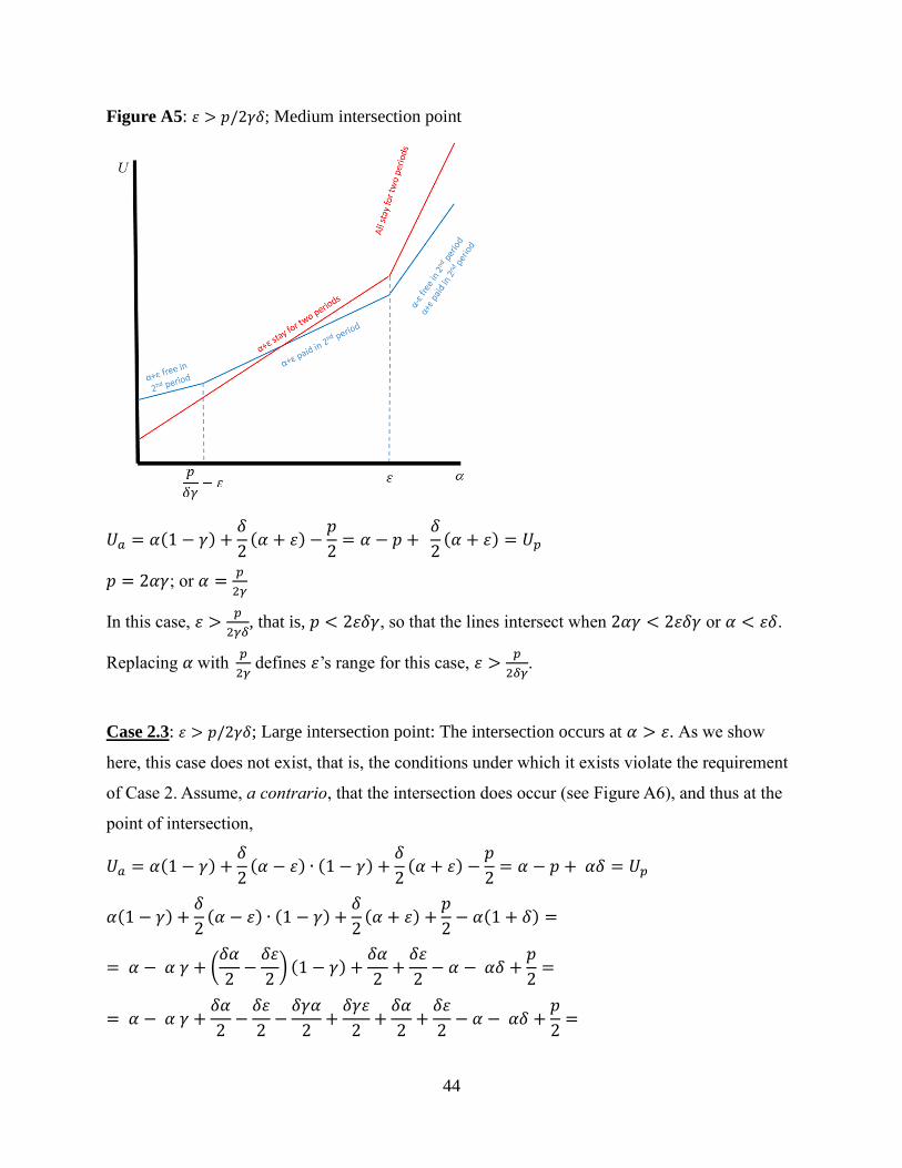
44

Figure A5: 휀 > 𝑝/2𝛾𝛿; Medium intersection point

𝑈𝑎 = 𝛼(1 − 𝛾) +𝛿

2(𝛼 + 휀) −

𝑝

2= 𝛼 − 𝑝 +

𝛿

2(𝛼 + 휀) = 𝑈𝑝

𝑝 = 2𝛼𝛾; or 𝛼 =𝑝

2𝛾

In this case, 휀 >𝑝

2𝛾𝛿, that is, 𝑝 < 2휀𝛿𝛾, so that the lines intersect when 2𝛼𝛾 < 2휀𝛿𝛾 or 𝛼 < 휀𝛿.

Replacing 𝛼 with 𝑝

2𝛾 defines 휀’s range for this case, 휀 >

𝑝

2𝛿𝛾.

Case 2.3: 휀 > 𝑝/2𝛾𝛿; Large intersection point: The intersection occurs at 𝛼 > 휀. As we show

here, this case does not exist, that is, the conditions under which it exists violate the requirement

of Case 2. Assume, a contrario, that the intersection does occur (see Figure A6), and thus at the

point of intersection,

𝑈𝑎 = 𝛼(1 − 𝛾) +𝛿

2(𝛼 − 휀) ∙ (1 − 𝛾) +

𝛿

2(𝛼 + 휀) −

𝑝

2= 𝛼 − 𝑝 + 𝛼𝛿 = 𝑈𝑝

𝛼(1 − 𝛾) +𝛿

2(𝛼 − 휀) ∙ (1 − 𝛾) +

𝛿

2(𝛼 + 휀) +

𝑝

2− 𝛼(1 + 𝛿) =

= 𝛼 − 𝛼 𝛾 + (𝛿𝛼

2−𝛿휀

2) (1 − 𝛾) +

𝛿𝛼

2+𝛿휀

2− 𝛼 − 𝛼𝛿 +

𝑝

2=

= 𝛼 − 𝛼 𝛾 +𝛿𝛼

2−𝛿휀

2−𝛿𝛾𝛼

2+𝛿𝛾휀

2+𝛿𝛼

2+𝛿휀

2− 𝛼 − 𝛼𝛿 +

𝑝

2=

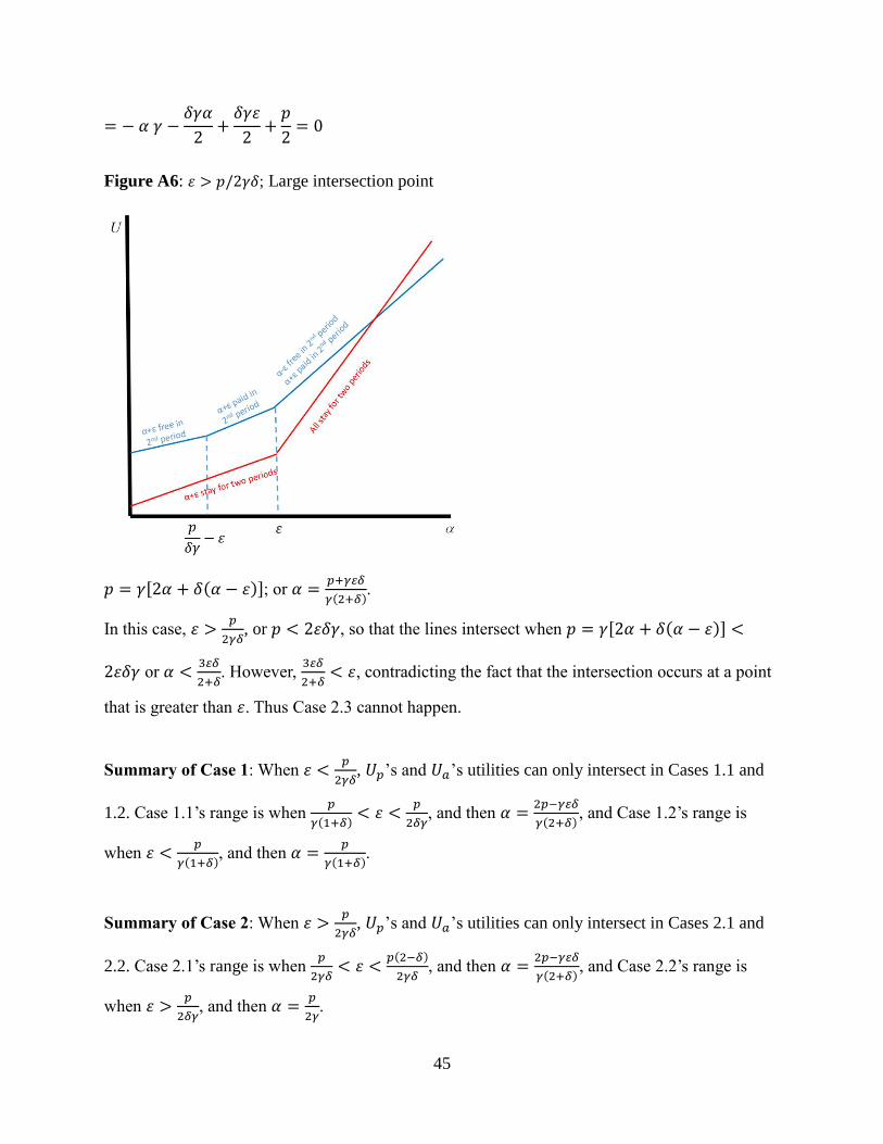
45

= − 𝛼 𝛾 −𝛿𝛾𝛼

2+𝛿𝛾휀

2+𝑝

2= 0

Figure A6: 휀 > 𝑝/2𝛾𝛿; Large intersection point

𝑝 = 𝛾[2𝛼 + 𝛿(𝛼 − 휀)]; or 𝛼 =𝑝+𝛾 𝛿

𝛾(2+𝛿).

In this case, 휀 >𝑝

2𝛾𝛿, or 𝑝 < 2휀𝛿𝛾, so that the lines intersect when 𝑝 = 𝛾[2𝛼 + 𝛿(𝛼 − 휀)] <

2휀𝛿𝛾 or 𝛼 <3 𝛿

2+𝛿. However,

3 𝛿

2+𝛿< 휀, contradicting the fact that the intersection occurs at a point

that is greater than 휀. Thus Case 2.3 cannot happen.

Summary of Case 1: When 휀 <𝑝

2𝛾𝛿, 𝑈𝑝’s and 𝑈𝑎’s utilities can only intersect in Cases 1.1 and

1.2. Case 1.1’s range is when 𝑝

𝛾(1+𝛿)< 휀 <

𝑝

2𝛿𝛾, and then 𝛼 =

2𝑝−𝛾 𝛿

𝛾(2+𝛿), and Case 1.2’s range is

when 휀 <𝑝

𝛾(1+𝛿), and then 𝛼 =

𝑝

𝛾(1+𝛿).

Summary of Case 2: When 휀 >𝑝

2𝛾𝛿, 𝑈𝑝’s and 𝑈𝑎’s utilities can only intersect in Cases 2.1 and

2.2. Case 2.1’s range is when 𝑝

2𝛾𝛿< 휀 <

𝑝(2−𝛿)

2𝛾𝛿, and then 𝛼 =

2𝑝−𝛾 𝛿

𝛾(2+𝛿), and Case 2.2’s range is

when 휀 >𝑝

2𝛿𝛾, and then 𝛼 =

𝑝

2𝛾.

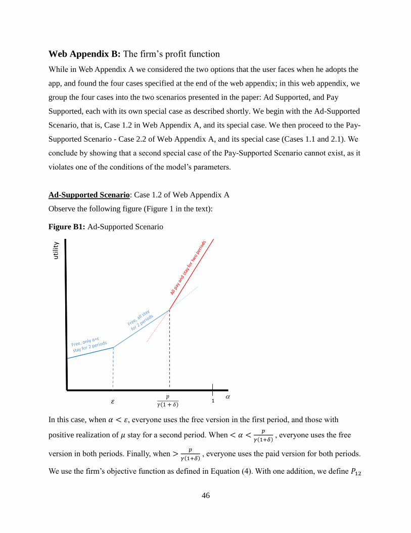
46

Web Appendix B: The firm’s profit function

While in Web Appendix A we considered the two options that the user faces when he adopts the

app, and found the four cases specified at the end of the web appendix; in this web appendix, we

group the four cases into the two scenarios presented in the paper: Ad Supported, and Pay

Supported, each with its own special case as described shortly. We begin with the Ad-Supported

Scenario, that is, Case 1.2 in Web Appendix A, and its special case. We then proceed to the Pay-

Supported Scenario - Case 2.2 of Web Appendix A, and its special case (Cases 1.1 and 2.1). We

conclude by showing that a second special case of the Pay-Supported Scenario cannot exist, as it

violates one of the conditions of the model’s parameters.

Ad-Supported Scenario: Case 1.2 of Web Appendix A

Observe the following figure (Figure 1 in the text):

Figure B1: Ad-Supported Scenario

In this case, when 𝛼 < 휀, everyone uses the free version in the first period, and those with

positive realization of 𝜇 stay for a second period. When < 𝛼 <𝑝

𝛾(1+𝛿) , everyone uses the free

version in both periods. Finally, when >𝑝

𝛾(1+𝛿) , everyone uses the paid version for both periods.

We use the firm’s objective function as defined in Equation (4). With one addition, we define 𝑃12

47

as the share of those who paid in Period 1 and stayed in Period 2: While they do not generate any

profit to the firm, and thus do not appear in Equation (4), we report their value here for

completeness’ sake.

Here, 𝑃1 = 𝑃12 = 1 −𝑝

𝛾(1+𝛿) ; 𝑃2 = 0; 𝐴1 =

𝑝

𝛾(1+𝛿) ; and 𝐴2 =

2𝑝−𝛾 (1+𝛿)

2𝛾(1+𝛿)

Π = 𝑝 (1 −𝑝

𝛾(1 + 𝛿) ) + 𝑘𝛾

4𝑝 − 𝛾휀(1 + 𝛿)

2𝛾(1 + 𝛿)− 𝛾2

Differentiating with respect to p, equating to zero and collecting terms yield:

𝑝𝑜𝑝𝑡 =𝛾

2(1 + 2𝑘 + 𝛿)

to be in this scenario requires 𝛾(1 + 𝛿) >𝛾

2(1 + 2𝑘 + 𝛿) > 휀𝛾(1 + 𝛿),

or: (휀 −1

2) (1 + 𝛿) < 𝑘 <

1+𝛿

2

Differentiating with respect to γ, equating to zero and collecting terms yield:

𝑝2

𝛾2(1 + 𝛿)−𝑘휀

2− 2𝛾 = 0

Substitute the optimal p from the above equation, and solve to get the optimal γ:

𝛾𝑜𝑝𝑡 =(1 + 2𝑘 + 𝛿)2 − 2𝑘휀(1 + 𝛿)

8(1 + 𝛿)

Now substitute𝛾𝑜𝑝𝑡 into 𝑝𝑜𝑝𝑡 to obtain the solution of optimal price as a function of the

parameters.

𝑝𝑜𝑝𝑡 = (1 + 2𝑘 + 𝛿)(1 + 2𝑘 + 𝛿)2 − 2𝑘휀(1 + 𝛿)

16(1 + 𝛿)

The optimal profits are then:

Π𝑜𝑝𝑡 =[(1 + 2𝑘 + 𝛿)2 − 2𝑘(1 + 𝛿)휀]2

64(1 + 𝛿)2

The partial derivatives of the optimal advertising, price, and profit levels are:

𝜕𝛾

𝜕휀= −

𝑘

4< 0

𝜕𝛾

𝜕𝛿=

(1+𝛿)2−4𝑘2

8(1+𝛿)2≥ 0, since

1+𝛿

2> 𝑘

𝜕𝛾

𝜕𝑘=2 − 휀

4+

𝑘

(1 + 𝛿)> 0

𝜕𝑝

𝜕휀= −

𝑘(1 + 2𝑘 + 𝛿)

8< 0

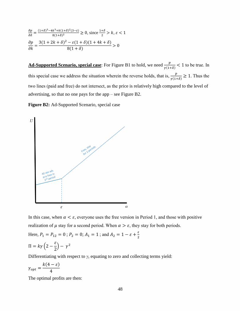
48

𝜕𝑝

𝜕𝛿=

(1+𝛿)3−4𝑘3+𝑘(1+𝛿)2(3− )

8(1+𝛿)2≥ 0, since

1+𝛿

2> 𝑘, 휀 < 1

𝜕𝑝

𝜕𝑘=3(1 + 2𝑘 + 𝛿)2 − 휀(1 + 𝛿)(1 + 4𝑘 + 𝛿)

8(1 + 𝛿)> 0

Ad-Supported Scenario, special case: For Figure B1 to hold, we need 𝑝

𝛾(1+𝛿)< 1 to be true. In

this special case we address the situation wherein the reverse holds, that is, 𝑝

𝛾(1+𝛿)≥ 1. Thus the

two lines (paid and free) do not intersect, as the price is relatively high compared to the level of

advertising, so that no one pays for the app – see Figure B2.

Figure B2: Ad-Supported Scenario, special case

In this case, when 𝛼 < 휀, everyone uses the free version in Period 1, and those with positive

realization of 𝜇 stay for a second period. When 𝛼 > 휀, they stay for both periods.

Here, 𝑃1 = 𝑃12 = 0 ; 𝑃2 = 0; 𝐴1 = 1 ; and 𝐴2 = 1 − 휀 +2

Π = 𝑘𝛾 (2 −휀

2) − 𝛾2

Differentiating with respect to γ, equating to zero and collecting terms yield:

𝛾𝑜𝑝𝑡 =𝑘(4 − 휀)

4

The optimal profits are then:

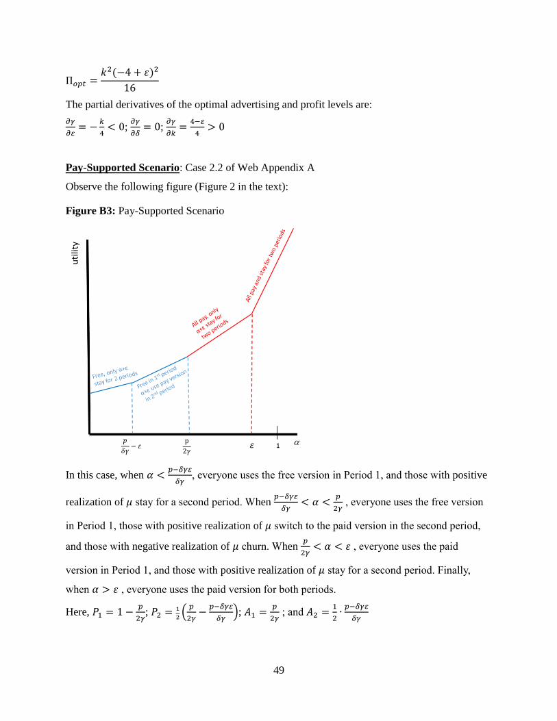
49

Π𝑜𝑝𝑡 =𝑘2(−4 + 휀)2

16

The partial derivatives of the optimal advertising and profit levels are:

𝜕𝛾

𝜕= −

𝑘

4< 0;

𝜕𝛾

𝜕𝛿= 0;

𝜕𝛾

𝜕𝑘=

4−

4> 0

Pay-Supported Scenario: Case 2.2 of Web Appendix A

Observe the following figure (Figure 2 in the text):

Figure B3: Pay-Supported Scenario

In this case, when 𝛼 <𝑝−𝛿𝛾

𝛿𝛾, everyone uses the free version in Period 1, and those with positive

realization of 𝜇 stay for a second period. When 𝑝−𝛿𝛾

𝛿𝛾< 𝛼 <

𝑝

2𝛾 , everyone uses the free version

in Period 1, those with positive realization of 𝜇 switch to the paid version in the second period,

and those with negative realization of 𝜇 churn. When 𝑝

2𝛾< 𝛼 < 휀 , everyone uses the paid

version in Period 1, and those with positive realization of 𝜇 stay for a second period. Finally,

when 𝛼 > 휀 , everyone uses the paid version for both periods.

Here, 𝑃1 = 1 −𝑝

2𝛾; 𝑃2 =

1

2(𝑝

2𝛾−𝑝−𝛿𝛾

𝛿𝛾); 𝐴1 =

𝑝

2𝛾 ; and 𝐴2 =

1

2∙𝑝−𝛿𝛾

𝛿𝛾

50

𝑃12 = 1 − 휀 +1

2(휀 −

𝑝

2𝛾) = 1 −

𝑝

4𝛾−휀

2

Π = 𝑝 (1 −𝑝

2𝛾) +

𝑝

2(𝑝

2𝛾−𝑝 − 𝛿𝛾휀

𝛿𝛾) + 𝑘𝛾

𝑝

2𝛾+𝑘𝛾(𝑝 − 𝛿𝛾휀)

2𝛿𝛾− 𝛾2

Differentiating with respect to p, equating to zero and collecting terms yield:

𝑝𝑜𝑝𝑡 =𝛾[𝑘(1+𝛿)+𝛿(2+ )]

2+𝛿 ;

Differentiating with respect to 𝛾, equating to zero and collecting terms yield:

1

4[𝑝2(2 + 𝛿)

𝛾2𝛿− 2𝑘휀 − 8𝛾] = 0

Substitute the optimal p from the above equation, and solve to get the optimal γ:

𝛾𝑜𝑝𝑡 =𝑘2(1 + 𝛿)2 + 2𝑘𝛿(2 + 2𝛿 − 휀) + 𝛿2(2 + 휀)2

8𝛿(2 + 𝛿)

Now substitute 𝛾𝑜𝑝𝑡 into 𝑝𝑜𝑝𝑡 to obtain the solution of optimal price as a function of the

parameters.

𝑝𝑜𝑝𝑡 =[𝑘(1 + 𝛿) + 𝛿(2 + 휀)][𝑘2(1 + 𝛿)2 + 2𝑘𝛿(2 + 2𝛿 − 휀) + 𝛿2(2 + 휀)2]

8𝛿(2 + 𝛿)2

The optimal profits are then:

Π𝑜𝑝𝑡 =([𝑘 + (2 + 𝑘)𝛿]2 − 2(𝑘 − 2𝛿)𝛿휀 + 𝛿2휀2)2

64𝛿2(2 + 𝛿)2

The partial derivatives of the optimal advertising and price levels are:

𝜕𝛾

𝜕휀=𝛿(2 + 휀) − 𝑘

4(2 + 𝛿)> 0

𝜕𝛾

𝜕𝛿=[𝛿(2 + 휀) − 𝑘][𝑘(1 + 𝛿) + 𝛿(2 + 휀)]

4𝛿2(2 + 𝛿)2> 0

𝜕𝛾

𝜕𝑘=(1 + 𝛿)[𝑘 + 𝛿(2 + 𝑘)] − 𝛿휀

4𝛿(2 + 𝛿)> 0

For the following three derivatives, we show that they are positive using numerical simulations,

wherein the derivatives are always positive for 𝛿 values that match the numerical simulations’

solutions as described in section 4 of the paper.

𝜕𝑝

𝜕휀= 𝑘2(𝛿2 − 1) + 3𝛿2(2 + 휀)2 + 2𝑘𝛿[2 − 휀 + 𝛿(4 + 휀)]

8(2 + 𝛿)2> 0

𝜕𝑝

𝜕𝛿=𝑘3(𝛿 − 2)(1 + 𝛿)2 + 4𝛿3(2 + 휀)3 + 𝑘𝛿2(2 + 휀)(12 + 18𝛿 − 2휀 + 5𝛿휀) + 2𝑘2𝛿2[6 + 휀 + 2𝛿(3 + 휀)]

8𝛿2(2 + 𝛿)3> 0

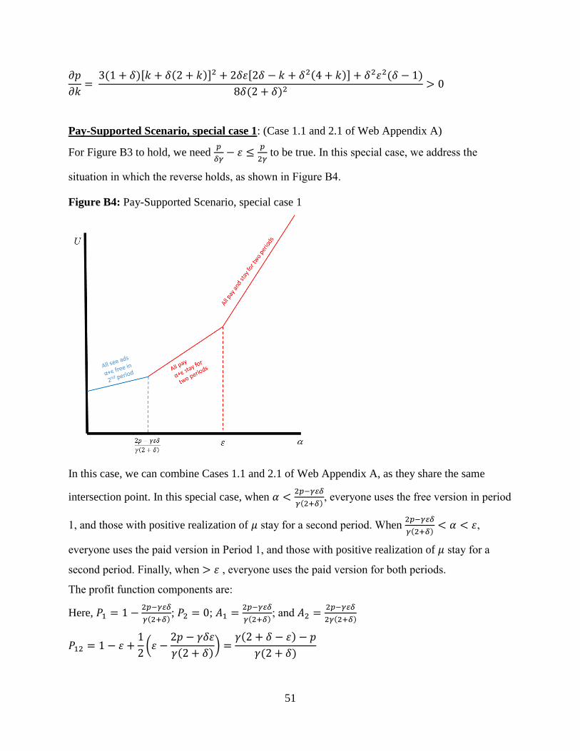
51

𝜕𝑝

𝜕𝑘= 3(1 + 𝛿)[𝑘 + 𝛿(2 + 𝑘)]2 + 2𝛿휀[2𝛿 − 𝑘 + 𝛿2(4 + 𝑘)] + 𝛿2휀2(𝛿 − 1)

8𝛿(2 + 𝛿)2> 0

Pay-Supported Scenario, special case 1: (Case 1.1 and 2.1 of Web Appendix A)

For Figure B3 to hold, we need 𝑝

𝛿𝛾− 휀 ≤

𝑝

2𝛾 to be true. In this special case, we address the

situation in which the reverse holds, as shown in Figure B4.

Figure B4: Pay-Supported Scenario, special case 1

In this case, we can combine Cases 1.1 and 2.1 of Web Appendix A, as they share the same

intersection point. In this special case, when 𝛼 <2𝑝−𝛾 𝛿

𝛾(2+𝛿), everyone uses the free version in period

1, and those with positive realization of 𝜇 stay for a second period. When 2𝑝−𝛾 𝛿

𝛾(2+𝛿)< 𝛼 < 휀,

everyone uses the paid version in Period 1, and those with positive realization of 𝜇 stay for a

second period. Finally, when > 휀 , everyone uses the paid version for both periods.

The profit function components are:

Here, 𝑃1 = 1 −2𝑝−𝛾 𝛿

𝛾(2+𝛿); 𝑃2 = 0; 𝐴1 =

2𝑝−𝛾 𝛿

𝛾(2+𝛿); and 𝐴2 =

2𝑝−𝛾 𝛿

2𝛾(2+𝛿)

𝑃12 = 1 − 휀 +1

2(휀 −

2𝑝 − 𝛾𝛿휀

𝛾(2 + 𝛿)) =

𝛾(2 + 𝛿 − 휀) − 𝑝

𝛾(2 + 𝛿)

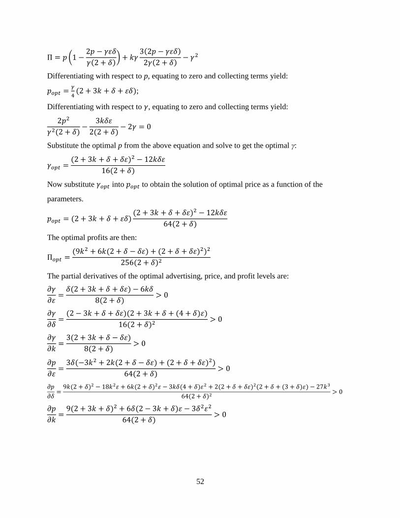
52

Π = 𝑝 (1 −2𝑝 − 𝛾휀𝛿

𝛾(2 + 𝛿)) + 𝑘𝛾

3(2𝑝 − 𝛾휀𝛿)

2𝛾(2 + 𝛿)− 𝛾2

Differentiating with respect to p, equating to zero and collecting terms yield:

𝑝𝑜𝑝𝑡 =𝛾

4(2 + 3𝑘 + 𝛿 + 휀𝛿);

Differentiating with respect to 𝛾, equating to zero and collecting terms yield:

2𝑝2

𝛾2(2 + 𝛿)−

3𝑘𝛿휀

2(2 + 𝛿)− 2𝛾 = 0

Substitute the optimal p from the above equation and solve to get the optimal γ:

𝛾𝑜𝑝𝑡 =(2 + 3𝑘 + 𝛿 + 𝛿휀)2 − 12𝑘𝛿휀

16(2 + 𝛿)

Now substitute 𝛾𝑜𝑝𝑡 into 𝑝𝑜𝑝𝑡 to obtain the solution of optimal price as a function of the

parameters.

𝑝𝑜𝑝𝑡 = (2 + 3𝑘 + 𝛿 + 휀𝛿)(2 + 3𝑘 + 𝛿 + 𝛿휀)2 − 12𝑘𝛿휀

64(2 + 𝛿)

The optimal profits are then:

Π𝑜𝑝𝑡 =(9𝑘2 + 6𝑘(2 + 𝛿 − 𝛿휀) + (2 + 𝛿 + 𝛿휀)2)2

256(2 + 𝛿)2

The partial derivatives of the optimal advertising, price, and profit levels are:

𝜕𝛾

𝜕휀=𝛿(2 + 3𝑘 + 𝛿 + 𝛿휀) − 6𝑘𝛿

8(2 + 𝛿)> 0

𝜕𝛾

𝜕𝛿=(2 − 3𝑘 + 𝛿 + 𝛿휀)(2 + 3𝑘 + 𝛿 + (4 + 𝛿)휀)

16(2 + 𝛿)2> 0

𝜕𝛾

𝜕𝑘=3(2 + 3𝑘 + 𝛿 − 𝛿휀)

8(2 + 𝛿)> 0

𝜕𝑝

𝜕휀=3𝛿(−3𝑘2 + 2𝑘(2 + 𝛿 − 𝛿휀) + (2 + 𝛿 + 𝛿휀)2)

64(2 + 𝛿)> 0

𝜕𝑝

𝜕𝛿=9𝑘(2 + 𝛿)2 − 18𝑘2휀 + 6𝑘(2 + 𝛿)2휀 − 3𝑘𝛿(4 + 𝛿)휀2 + 2(2 + 𝛿 + 𝛿휀)2(2 + 𝛿 + (3 + 𝛿)휀) − 27𝑘3

64(2 + 𝛿)2> 0

𝜕𝑝

𝜕𝑘=9(2 + 3𝑘 + 𝛿)2 + 6𝛿(2 − 3𝑘 + 𝛿)휀 − 3𝛿2휀2

64(2 + 𝛿)> 0

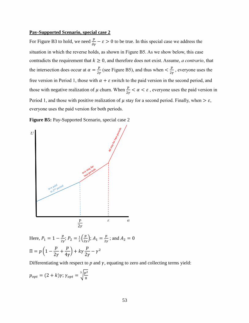
53

Pay-Supported Scenario, special case 2

For Figure B3 to hold, we need 𝑝

𝛿𝛾− 휀 > 0 to be true. In this special case we address the

situation in which the reverse holds, as shown in Figure B5. As we show below, this case

contradicts the requirement that 𝑘 ≥ 0, and therefore does not exist. Assume, a contrario, that

the intersection does occur at 𝛼 =𝑝

2𝛾 (see Figure B5), and thus when <

𝑝

2𝛾 , everyone uses the

free version in Period 1, those with 𝛼 + 휀 switch to the paid version in the second period, and

those with negative realization of 𝜇 churn. When 𝑝

2𝛾< 𝛼 < 휀 , everyone uses the paid version in

Period 1, and those with positive realization of 𝜇 stay for a second period. Finally, when > 휀,

everyone uses the paid version for both periods.

Figure B5: Pay-Supported Scenario, special case 2

Here, 𝑃1 = 1 −𝑝

2𝛾; 𝑃2 =

1

2(𝑝

2𝛾); 𝐴1 =

𝑝

2𝛾 ; and 𝐴2 = 0

Π = 𝑝 (1 −𝑝

2𝛾+𝑝

4𝛾) + 𝑘𝛾

𝑝

2𝛾− 𝛾2

Differentiating with respect to p and 𝛾, equating to zero and collecting terms yield:

𝑝𝑜𝑝𝑡 = (2 + 𝑘)𝛾; 𝛾𝑜𝑝𝑡 = √𝑝2

8

3

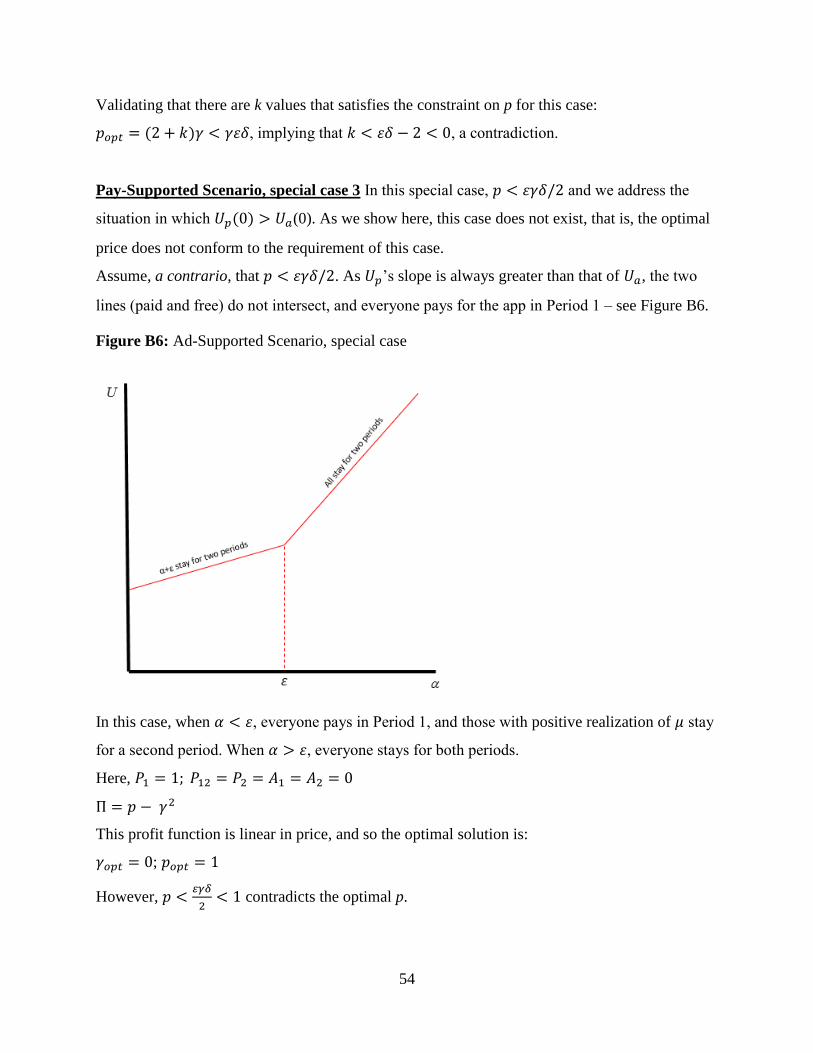
54

Validating that there are k values that satisfies the constraint on p for this case:

𝑝𝑜𝑝𝑡 = (2 + 𝑘)𝛾 < 𝛾휀𝛿, implying that 𝑘 < 휀𝛿 − 2 < 0, a contradiction.

Pay-Supported Scenario, special case 3 In this special case, 𝑝 < 휀𝛾𝛿/2 and we address the

situation in which 𝑈𝑝(0) > 𝑈𝑎(0). As we show here, this case does not exist, that is, the optimal

price does not conform to the requirement of this case.

Assume, a contrario, that 𝑝 < 휀𝛾𝛿/2. As 𝑈𝑝’s slope is always greater than that of 𝑈𝑎, the two

lines (paid and free) do not intersect, and everyone pays for the app in Period 1 – see Figure B6.

Figure B6: Ad-Supported Scenario, special case

In this case, when 𝛼 < 휀, everyone pays in Period 1, and those with positive realization of 𝜇 stay

for a second period. When 𝛼 > 휀, everyone stays for both periods.

Here, 𝑃1 = 1; 𝑃12 = 𝑃2 = 𝐴1 = 𝐴2 = 0

Π = 𝑝 − 𝛾2

This profit function is linear in price, and so the optimal solution is:

𝛾𝑜𝑝𝑡 = 0; 𝑝𝑜𝑝𝑡 = 1

However, 𝑝 <𝛾𝛿

2< 1 contradicts the optimal p.

55

Web Appendix C: Profits and uncertainty

In this appendix we show the conditions under which profits are increasing under uncertainty (휀).

Pay-Supported Scenario (main case)

The optimal profits are given by (see Web Appendix B):

Π𝑜𝑝𝑡 =([𝑘 + (2 + 𝑘)𝛿]2 − 2(𝑘 − 2𝛿)𝛿휀 + 𝛿2휀2)2

64𝛿2(2 + 𝛿)2

∂Π𝑜𝑝𝑡/𝜕휀 =2([𝑘 + (2 + 𝑘)𝛿]2 − 2(𝑘 − 2𝛿)𝛿휀 + 𝛿2휀2)1

64𝛿2(2 + 𝛿)2𝐴

Where

𝐴 = −2(𝑘 − 2𝛿)𝛿 + 2𝛿2ε = 2δ(−k + 2δ + δε)

∂Π𝑜𝑝𝑡/𝜕휀 is positive if

𝑘 < 𝛿(2 + 휀)

Pay-Supported Scenario (special case 1)

The optimal profits are given by (see Web Appendix B):

Π𝑜𝑝𝑡 =(9𝑘2 + 6𝑘(2 + 𝛿 − 𝛿휀) + (2 + 𝛿 + 𝛿휀)2)2

256(2 + 𝛿)2

∂Π𝑜𝑝𝑡/𝜕휀 =2(9𝑘2 + 6𝑘(2 + 𝛿 − 𝛿휀) + (2 + 𝛿 + 𝛿휀)2)1

256(2 + 𝛿)2𝐵

where

𝐵 = −6𝑘𝛿 + 2(2 + 𝛿 + 𝛿휀)1𝛿 = 2𝛿(−3𝑘 + 2 + 𝛿 + 휀𝛿)

∂Π𝑜𝑝𝑡/𝜕휀 is positive if

𝑘 <2 + 𝛿(1 + 휀)

3

Numerical simulation of these two cases reveals that in all value parameters of the pay-supported

scenario (main case), indeed 𝑘 < 𝛿(2 + 휀), while in the special case, 𝑘 ≤ (2 + 𝛿(1 + 휀))/3.