on nash dynamics of matching market equilibria
TRANSCRIPT
arX
iv:1
103.
4196
v1 [
cs.G
T]
22
Mar
201
1
On Nash Dynamics of Matching Market Equilibria
Ning Chen∗ Xiaotie Deng†
∗Division of Mathematical Sciences, Nanyang Technological University, Singapore.Email: [email protected]
†Department of Computer Science, University of Liverpool, UK.Email: [email protected]
Abstract
In this paper, we study the Nash dynamics of strategic interplays of n buyers in a matching marketsetup by a seller, the market maker. Taking the standard market equilibrium approach, upon receivingsubmitted bid vectors from the buyers, the market maker will decide on a price vector to clear themarket in such a way that each buyer is allocated an item for which he desires the most (a.k.a., a marketequilibrium solution). While such equilibrium outcomes are not unique, the market maker chooses one(max-eq) that optimizes its own objective — revenue maximization. The buyers in turn change bids totheir best interests in order to obtain higher utilities in the next round’s market equilibrium solution.
This is an (n+ 1)-person game where buyers place strategic bids to gain the most from the marketmaker’s equilibrium mechanism. The incentives of buyers in deciding their bids and the market maker’schoice of using the max-eq mechanism create a wave of Nash dynamics involved in the market. Wecharacterize Nash equilibria in the dynamics in terms of the relationship between max-eq and min-eq (i.e., minimum revenue equilibrium), and develop convergence results for Nash dynamics from themax-eq policy to a min-eq solution, resulting an outcome equivalent to the truthful VCG mechanism.
Our results imply revenue equivalence between max-eq and min-eq, and address the question thatwhy short-term revenue maximization is a poor long run strategy, in a deterministic and dynamic setting.

1 Introduction
The Nash equilibrium paradigm in Economics has been based on a rationality assumption that each individualwill maximize its own utility function. Making it further to a dynamic process where multiple agents playinteractively in a repeated game, the Nash dynamics refers to a process where participants take turnsto choose a strategy to maximize their own utility function. We pose the question of what impact ofsuch strategic behavior of the seller, as the market maker, can have on Nash dynamics of the buyers in amatching market setting [28], where the seller has m products and there are n unit-demand potential buyerswith different private values vij for different items.
We base our consideration on the market equilibrium framework: The market maker chooses a non-negative price vector and an allocation vector; the outcome is called a market competitive equilibrium ifall items with positive prices are sold out and everyone gets his maximum utility at the correspondingallocation, measured by the difference between the buyer’s value of the item and the charged price, i.e.,vij − pj. To achieve its own objective, i.e., revenue maximization, the market maker is naturally to set allitems the highest possible prices so that there is still a supported allocation vector that clears the marketand maximizes everyone’s utility. This yields a seller-optimal outcome and is called a maximum competitiveequilibrium. Alternatively, at another extreme, the outcome of the market can be buyers-optimal, i.e., aminimum competitive equilibrium where all items have the lowest possible prices to ensure market clearanceand utility maximization. Maximum and minimum equilibria represent the contradictory interests of thetwo parties in a two-sided matching market at the two extremes; and, as shown by Shapley and Shubik [28],both equilibria always exist and their prices are unique.
Using market equilibrium as a mechanism for computing prices and allocations yields desirable propertiesof efficiency and fairness. The winners in the mechanism, however, will bid against the protocol to reducetheir payments; further, the losers may increase their bids to be more competitive (to their best interests).The problem becomes an (n+1)-person game played in turn between the seller and the buyers where buyersmake strategic moves to (mis)report their bids for the items, in response to other buyers’ bids and thesolution selected by the market maker.
It is well-known that the minimum equilibrium mechanism admits a truthful dominant strategy forevery buyer [22, 8], resulting in a solution equivalent to the VCG protocol [30, 5, 15]. However, it ishardly convincing a rational economic agent who dominates the market to make a move that maximizes thecollective returns of its buyers by sacrificing its own revenue. Clearly, the Nash equilibrium paradigm hasalways assumed that an economic agent is a utility maximizer; for the market marker, it implies revenuemaximization. Further, success in bringing great revenue (in a short term) will bring a large number ofeyeballs and lead to positive externalities, which could breed more success (in a long term). Indeed, quite afew successful designs, like the generalized second price auction for sponsored search markets [1] and the FCCspectrum auction for licenses of electromagnetic spectra [6, 23], do not admit a truthful dominant strategy.
Our interest is to find out the properties of the game between the seller and the buyers (among whichthey compete with each other for the items), especially with these two extremes of the solution concepts —their relationship proves to be significant in the incentive analysis of the buyers in the market. In particular,we are interested in the dynamics of the outcomes when the market maker adopts the maximum equilibriummechanism and the buyers adopt a particular type of strategy, that of the best response strategy. With thebest response strategy, a buyer would announce his bids for all items that would result in the maximumutility for himself, under the fixed bids of other buyers and the maximum equilibrium mechanism prefixedby the market maker. The best response strategy varies depending on the circumstances of the market andhas its nature place in the analysis of dynamics of strategic interplays of agents.
For the special case of single item markets where the market maker has only one item to sell, maximumequilibrium corresponds to the first price auction protocol and minimum equilibrium corresponds to thesecond price auction protocol. The first price auction sells the item to the buyer with the highest bid ata price equal to his bid (i.e., the highest possible price so that everyone is happy with his correspondingallocation). Under a dynamic setting, buyers take turns in making their moves in response to what they areencountered in the previous round(s). In a simple setting when all buyers bid their true values initially, thewinner with the highest bid will immediately shade his bid down to the smallest value so that he is still a
1

winner. Such best response bidding of the winner results in an outcome equivalent to the Vickrey secondprice auction, which charges the winner at the smallest possible price (i.e., the second highest bid) so thateveryone’s utility is maximized. The observation of convergence from the first price to the second price goeshand-in-hand with the seminal revenue equivalence theory in Bayesian analysis [30, 26]. Therefore, both theBayesian model and the dynamic best response model point to the same unification result of the first priceand the second price solution concepts in the single item markets.
The story is hardly ending for the process of Nash dynamics with multiple items being sold in the market,which illustrates a rich structure that a single item market does not possess. First of all, in a single itemmarket, the best response decision of a buyer is binary, that is, he decides either to or not to compete withthe highest bid of others for the item at a smallest cost. With multiple items, however, a buyer needs tomake his decision in the best response over all items rather than a single item. In particular, he may desireany item in a subset — each of which brings him the same maximum utility — and lose interest for otheritems. The buyer’s best response, therefore, is in accordance with his strategic bids for the items in bothsubsets. For example, it is possible that one increases hid bid for one item but decreases for another in a bestresponse. This opens many possibilities that would complicate the analysis; in particular, best responses ofa buyer are not unique. Indeed, as Example 3.1 shows, not all best responses guarantee convergence, againbecause of the multiplicity in possibilities of bidding strategies.
Second, in a single item market, the submitted bids of buyers illustrate a monotone property to the priceof the item. That is, when a buyer increases his bid, the price is always monotonically non-decreasing. Withmultiple items, while it is true that the prices of the items are still monotone with respect to the bids ofthe losers, counter-intuitively, the prices are no longer monotone with respect to the bids of the winners,as the following Example 1.1 shows. This non-monotonicity further requires extra efforts to analyze themultiplicity of best response strategies and their properties.
Example 1.1 (Non-monotonicity). There are three buyers i1, i2, i3 and two items j1, j2 with submitted bidsbi1j1 = 2, bi2j1 = 12, bi2j2 = 14 and bi3j2 = 5 (the bids of all unspecified pairs are zero). For the givenbid vector, (pj1 , pj2) = (3, 5) is the maximum equilibrium price vector, and assigning j1 to i2 and j2 to i3are supported allocations. If a winner i2 increases his bid of j2 to b′i2j2 = 15, then (p′j1 , p
′j2) = (2, 5) is the
maximum equilibrium price vector (with the same allocations) where the price of j1 is decreased from 3 to 2.Hence, the maximum equilibrium prices are not monotone with respect to the submitted bids (of the winners).
Finally, the maximum market equilibrium solution has no closed form as in the single item case, andthe convergence of the best responses depends on a careful choice of the bidding strategy. Recall that amajor difficulty in analyzing the best responses is that, in addition to bidding strategically for the itemsthat bring the maximum utility, buyers may have (almost arbitrarily) different bidding strategies for thoseitems that they are not interested in; these decisions indeed play a critical role to the convergence of the bestresponses. As not all best responses necessarily lead to convergence (Example 3.1), we restrict to a specificbidding strategy, called aligned best response, where a bid vector of a buyer is called aligned if any allocationof an item with positive bid brings him the maximum utility. The aligned bidding strategy illustrates thepreference of a buyer over all items and is shown to be a best response (Lemma 3.1 and 3.2). While thealigned best response still does not have a monotone property in general (see Figure 3), the prices do exhibita pattern of monotonicity when the bids of the buyers have already been aligned. Based on these properties,we show that the aligned best response always converges and maximizes social welfare, summarized by thefollowing claim.
Theorem. In the maximum competitive equilibrium mechanism game, for any initial bid vector and anyordering of the buyers, the aligned best response always converges. Further, the allocation at convergencemaximizes social welfare.
In addition to proving convergence, another important question is that which Nash equilibrium to whichthe best response will converge. In contrast with single item markets where Nash equilibrium is essentiallyunique, in multi-item markets there can be several Nash equilibria with completely irrelevant price vectors(see Appendix D); this is another remarkable difference between single item and multi-item markets. Despite
2
of the multiplicity of Nash equilibria, if we start with an aligned bid vector (e.g., bid truthfully), the bestresponse always converges to one at a minimum competitive equilibrium, i.e., a VCG outcome.
Theorem. Starting from an aligned bid vector, the aligned best response of the maximum equilibriummechanism converges to a minimum competitive equilibrium at truthful bidding.
1.1 Related Work and Motivation
The study of competitive equilibrium in a matching market was initiated by Shapley and Shubik in anassignment model [28]. They showed that maximum and minimum competitive equilibria always exist andgave a simple linear program to compute one. Their results were later improved to the models with generalutility functions [7, 13]. Leonard [22] and Demange and Gale [8] studied strategic behaviors in the marketand proved that the minimum equilibrium mechanism admits a truthful dominant strategy for every buyer.Later, Demange, Gale and Sotomayor [9] gave an ascending auction based algorithm that converges to aminimum equilibrium. Our study focuses on Nash dynamics in the matching market model; the convergencefrom maximum equilibrium to minimum equilibrium implies revenue equivalence, and addresses the questionthat why short-term revenue maximization is a poor long run strategy in a dynamic framework.
The Nash dynamics of best responses has its nature place in the analysis of interplays of strategic agents.In general, characterizing equilibria of the dynamics is difficult or intractable. There have been extensivestudies in the literature for some special settings, e.g., potential games [25], congestion games [4], evolutionarygames [18], concave games [11], correlated equilibrium [17], sink equilibria [14], and market equilibrium [31],to name a few. Complexity issues have also been addressed in the analysis of best responses [2, 12, 25].Recently, Nisan et al. [27] independently considered best response dynamics in matching market and showa similar convergence result for running first price auctions for all items individually. To the best of ourknowledge, our work is the first to study best response dynamics in the maximum competitive equilibriummechanism.
Despite the motivation is mainly from theoretical curiosity, our setting does capture some realistic ap-plications, such as eBay electronic market and sponsored search market, which have attracted a lot researchefforts in recent years. The mechanism used in the sponsored search market is that of the generalized secondprice (GSP) auction. Because GSP is not truthful in general, a number of studies have focused on strategicconsiderations of advertisers. Edelman et al. [10] and Varian [29] independently showed that certain Nashequilibrium in the GSP auction derives the same revenue as the well-known truthful VCG scheme. Cary etal. [3] showed that a certain best response bidding strategy converges to the best Nash equilibrium. Recently,Leme and Tardos [21] considered other possible Nash equilibrium outputs and showed that the ratio betweenthe worst and best Nash equilibria is upper bounded by 1.618. These results putting together illustrate apretty complete overview of the structure of strategic behaviors in GSP. Our results are not directly aboutGSP but in a different way to reconfirm the revenue equivalence: While the search engine may adopt adifferent protocol with the goal of revenue maximization (i.e., the maximum equilibrium mechanism), withrational advertisers its overall revenue will eventually be the same as in the VCG protocol.
Another widely studied problem related to our model is that of spectrum markets. In designing theFCC spectrum auction protocol, a multiple stage bidding process, proposed by Milgrom [23], to digestcoordination, optimization and withdrawal, is adopted. It is conducted in several stages to allow buyers tochange their bids when the seller announces the tentative prices of the licenses for the winners. Therefore,it is created as an alternative game played between the seller and the buyers as a whole. Our best responseanalysis considers the dynamic aspect of the model and illustrates the convergence of the dynamic process.
Organization. We will first describe our model and maximum/minimum competitive equilibrium (mech-anism) in Section 2. In Section 3, we define the aligned bidding strategy and show that it is a best responseand always converges. In Section 4, we characterize Nash equilibria in the maximum equilibrium mechanismgame; and based on the characterization, we show that the maximum equilibrium mechanism converges toa minimum equilibrium output. We conclude our discussions in Section 5.
3

2 Preliminaries
We have a market with n unit-demand buyers, where each buyer wants at most one item, and m indivisibleitems, where each item can be sold to at most one buyer. We will denote buyers by i and items by jthroughout the paper. For every buyer i and item j, there is a value vij ∈ [0,∞), representing the maximumamount that i is willing to pay for item j. We will assume that there are m dummy buyers all with valuezero for each item j, i.e., vij = 0. This assumption is without loss of generality, and implies that the numberof items is always less than or equal to the number of buyers, i.e., m ≤ n.
The outcome of the market is a tuple (p,x), where
• p = (p1, . . . , pm) ≥ 0 is a price vector, where pj is the price charged for item j;
• x = (x1, . . . , xn) is an allocation vector, where xi is the item that i wins. If i does not win any items,denote xi = ∅. Note that different buyers must win different items, i.e., xi 6= xi′ for any i 6= i′ ifxi, xi′ 6= ∅.
Given an output (p,x), let ui(p,x) denote the utility that i obtains. We will assume that all buyers havequasi-linear utilities. That is, if i wins item j (i.e., xi = j), his utility is ui(p,x) = vij − pj; if i does not winany item (i.e., xi = ∅), his utility is ui(p,x) = 0.
Buyers’ preferences over items are according to their utilities — higher utility items are more preferable.We say that buyer i (strictly) prefers j to j′ if vij − pj > vij′ − pj′ , is indifferent between j and j′ ifvij − pj = vij′ − pj′ , and weakly prefers j to j′ if vij − pj ≥ vij′ − pj′ . In particular, a utility of zero,vij − pj = 0, means that i is indifferent between buying item j at price pj and not buying anything at all; anegative utility vij − pj < 0 means that the buyer strictly prefers to not buy the item at price pj .
We consider the following solution concept in this paper.
Definition 2.1. (Competitive equilibrium) We say a tuple (p,x) is a competitive equilibrium if (i) forany item j, pj = 0 if no one wins j in allocation x, and (ii) for any buyer i, his utility is maximized by hisallocation at the given price vector. That is,
• if i wins item j (i.e., xi = j), then vij − pj ≥ 0; and for every other item j′, vij − pj ≥ vij′ − pj′ ;
• if i does not win any item (i.e., xi = ∅), then for every item j, vij −pj ≤ 0. (For notational simplicity,we write vi∅ − p∅ = 0.)
The first condition above is an efficiency condition (i.e., market clearance), which says that all unallocateditems are priced at zero (or at some given reserve price). The assumption that there is a dummy buyer foreach item allows us to assume, without loss of generality, that all items are allocated in an equilibrium. Thesecond is a fairness condition (i.e., envy-freeness), implying that each buyer is allocated with an item thatmaximizes his utility at these prices. That is, if i wins item j, then i cannot obtain higher utility from anyother item; and if i does not win any item, then i cannot obtain a positive utility from any item. Namely,all buyers are happy with their corresponding allocations at the given price vector.
For any given matching market, Shapley and Shubik [28] proved that there always is a competitiveequilibrium. Actually, what they showed was much stronger — there is the unique minimum (respectively,maximum) equilibrium price vector, defined formally as follows.
Definition 2.2. (Minimum equilibrium min-eq and maximum equilibrium max-eq) A price vector p
is called a minimum equilibrium price vector if for any other equilibrium price vector q, pj ≤ qj for everyitem j. An equilibrium (p,x) is called a minimum equilibrium (denoted by min-eq) if p is the minimumequilibrium price vector. The maximum equilibrium price vector and a maximum equilibrium (denoted bymax-eq) are defined similarly.
For example, there are there buyers i1, i2, i3 and one item; the values of buyers are vi1 = 10, vi2 = 5 andvi3 = 2. Then p = 5 and p = 10 are the minimum and maximum equilibrium prices, respectively. Allocatingthe item to the first buyer i1, together with any price 5 ≤ p ≤ 10, yields a competitive equilibrium. When
4

there is a single item, it can be seen that the outcome of the minimum equilibrium and the maximumequilibrium corresponds precisely to the “second price auction” and the “first price auction”, respectively.
Consider another example: There are there buyers i1, i2, i3 and two items j1, j2; the values of buyers arevi1j1 = 10, vi1j2 = 6, vi2j1 = 8, vi2j2 = 4, and vi3j1 = 3, vi3j2 = 2. Then (6, 2) is the minimum equilibriumprice vector and (8, 4) is the maximum equilibrium price vector. Note that the allocation vectors supportedby the minimum or maximum equilibrium price vector may not be unique. In this example, we can allocatej1 and j2 arbitrarily to i1 and i2 to form an equilibrium. Indeed, as Gul and Stacchetti [16] showed, if bothp and q are equilibrium price vectors and (p,x) is a competitive equilibrium, then (q,x) is an equilibriumas well.
2.1 Maximum Equilibrium Mechanism Game
In this paper, we will consider a maximum equilibrium as a mechanism, that is, every buyer i reports a bid bijfor each item j (note that bij can be different from his true value vij), and given reported bids from all buyersb = (bij), the maximum equilibrium mechanism (again denoted by max-eq) outputs a maximum equilibriumwith respect to b. Let max-eq(b) denote the (maximum) equilibrium returned by the mechanism.
Let ui(b) denote the utility that i obtains in max-eq(b). That is, if (p,x) = max-eq(b), then ui(b) =vixi
−pxiif xi 6= ∅ and ui(b) = 0 if xi = ∅. Note that the (true) utility of every buyer is defined according to
his true valuations vij , rather than the bids bij ; and the “equilibrium” output (p,x) is computed in terms ofthe bid vector b, rather than the true valuations (i.e., it is only guaranteed that bixi
− pxi≥ bij − pj for any
item j). Therefore, the true utility of a buyer i might not be maximized at the corresponding allocation xi
and the given price vector p. Further, the output (p,x) = max-eq(b) might not even be a real equilibriumwith respect to the true valuations of the buyers.
Considering competitive equilibria as mechanisms defines a multi-parameter setting and it is naturalto consider strategic behaviors of the buyers. While it is a dominant strategy for every buyer to reporthis true valuations in the minimum equilibrium mechanism (i.e., the mechanism outputs a min-eq for thegiven bid vector) [8], the max-eq mechanism does not in general admit a dominant strategy. This istrue even for the degenerated single item case — it is well-known that the first price auction is not incentivecompatible. Therefore, in the max-eqmechanism, buyers will behave strategically to maximize their utilities.In particular, fixing bids of other buyers, buyer i will naturally place his bid vector (bij)j to maximize hisown utility; such a vector is called a best response. The focus of the present paper is to consider convergenceof best response dynamics, i.e., buyers iteratively change their bids according to best responses while all theothers remain their previous bids unchanged. We say a best response dynamics converges if it eventuallyreaches a state where no buyer is willing to change his bid anymore; hence, it arrives at a Nash equilibrium.
As our focus is on the convergence of best response dynamics, we discretize the bidding space of everybuyer to be a multiple of a given arbitrarily small constant ǫ > 0, and assume that all vij ’s and bij ’s aremultiples of ǫ. In practice, ǫ can be, e.g., one cent or one dollar (or any other unit number). This assumptionis natural in the context of two-sided markets with money transfers, and implies that if a buyer increases hisbid for an item, it must be by at least ǫ. In addition, we assume that the bid that every buyer submits forevery item is less than or equal to his true valuation, i.e., bij ≤ vij . This assumption is rather mild because(i) bidding higher than the true valuations carries the risk of a negative utility, and (ii) as Lemma 3.1 and3.2 below show, for any given fixed bids of other buyers, there always is a best response strategy for everybuyer to bid less than or equal to his true valuations.
2.2 Computation of Maximum Equilibrium
Shapley and Shubik [28] gave a linear program to compute a min-eq; their approach can be easily transformedto compute a max-eq by changing the objective to maximize the total payment. Next we give a combinatorialalgorithm to iteratively increase prices to converge to a max-eq. The idea of the algorithm is important toour analysis in the subsequent sections.
Definition 2.3 (Demand graph). Given any given bid vector b and price vector p, its demand graph
5

G(b,p) = (A,B;E) is defined as follows: A is the set of buyers and B is the set of items, and (i, j) ∈ E ifbij ≥ pj and bij − pj ≥ bij′ − pj′ for any j′.
In a demand graph G(b,p), every edge (i, j) represents that item j gives maximal utility to buyer i, pre-sumed that his true valuations are given by b. Note that demand graph is uniquely determined by the givenbid vector and price vector, and is independent to any allocation vector. However, an equilibrium allocationmust be selected from the set of edges in the demand graph. The following definition of alternating paths inthe demand graph is crucial to our analysis. (Recall that all items are allocated out in an equilibrium.)
Definition 2.4. (max-alternating path) Given any equilibrium (p,x) of a given bid b, let G = G(b,p)be its demand graph. For any item j, a path (j = j1, i1, j2, i2, . . . , jℓ, iℓ) in graph G is called a max-alternating path if edges are in and not in the allocation x alternatively, i.e., xik = jk for all k = 1, . . . , ℓ.Denote by Gmax
j (b,p,x) (or simply Gmaxj when the parameters are clear from the context) the subgraph of
G(b,p) (containing both buyers and items including j itself) reachable from j through max-alternating pathswith respect to x. A max-alternating path (j = j1, i1, j2, i2, . . . , jℓ, iℓ) in Gmax
j (b,p,x) is called critical ifbiℓjℓ = pjℓ .
For any given bid vector b, let (p,x) be an arbitrary equilibrium. Note that for any buyer i with xi 6= ∅,(i, xi) is an edge in the demand graph G(b,p). We consider the following recursive rule to increase prices:For any item j, increase prices of all items in Gmax
j continuously with the same amount until one of thefollowing events occurs:
1. There is buyer i ∈ Gmaxj such that bixi
= pxi(note that xi ∈ Gmax
j );
2. There is buyer i ∈ Gmaxj and item j′ /∈ Gmax
j such that i obtains maximal utility from j′ as well; thenwe add edge (i, j′) to the demand graph and update Gmax
j for each j.
The process continues iteratively until we cannot increase the price for any item. Denote the algorithm byAlg-max-eq. We have the following result.
Theorem 2.1. Starting from an arbitrary equilibrium (p,x) for the given bid vector b, let q be the finalprice vector in the above price-increment process Alg-max-eq. Together with the original allocation vectorx, (q,x) is a max-eq with respect to b.
The above algorithm Alg-max-eq and theorem illustrate the idea of defining Gmaxj (and the correspond-
ing max-alternating paths), summarized in the following corollary. (Note that if (j = j1, i1, j2, i2, . . . , jℓ, iℓ)is a critical max-alternating path in Gmax
j (b,p,x), then the last pair (iℓ, jℓ) where biℓjℓ = pjℓ is the exactreason that why we are not able to increase the price pj further in the Alg-max-eq to derive a higherequilibrium price vector.)
Corollary 2.1. Given any bid vector b and (p,x) = max-eq(b), for any item j, there is a critical max-alternating path in the subgraph Gmax
j (b,p,x).
3 Best Response Dynamics
For any given bid vector b, assume that the max-eq outputs (p,x), i.e., (p,x) = max-eq(b). If (p,x) isnot a Nash equilibrium, there is a buyer who is able to obtain more utility by unilaterally changing his bid.Such a buyer will therefore naturally choose a vector (called a best response) to bid so that his utility ismaximized in the max-eq mechanism, given fixed bids of all other buyers.
Consider the following example: There are three buyers i1, i2, i3 and two items j1, j2, with bi1j1 = vi1j1 =20, bi1j2 = vi1j2 = 18, and bi2j1 = bi2j2 = bi3j1 = bi3j2 = 10. Then p = (12, 10) is the maximum equilibriumprice and i1 obtains utility 8. Consider a scenario where i1 changes his bid to b′i1j1 = b′i1j2 = 15; then themaximum equilibrium price vector becomes p′ = (10, 10). Given the equilibrium price vector p′, however,there are two different equilibrium allocations which give him different true utilities (where i1 either wins j1
6
with utility vi1j1 − p′j1 = 10 or wins j2 with utility vi1j2 − p′j2 = 8). Hence, different selections of equilibriumallocations may lead to different true utilities, which in turn will certainly affect best response strategies ofthe buyers.
To analyze the best responses of the buyers, it is therefore necessary to specify a framework about theirbelief on the resulting equilibrium allocations. We will consider worst case analysis in this paper, i.e., allbuyers are risk-averse and always assume the worst possible allocations when making their best responses1.The above bid vector b′i1j1 = b′i1j2 = 15, therefore, is not a best response for i1 since his utility in the worstallocation is only 8. In the worse-case analysis framework, the best responses of i1 in the above example aregiven by b′i1j1 = 10 + ǫ and b′i1j2 ≤ 10 where i1 wins j1 at price 10 + ǫ with utility vi1j1 − (10 + ǫ) = 10 − ǫ(it can be seen that there is no bid vector such that i1 can obtain a utility higher than or equal to 10 givenfixed bids of the other two buyers)2.
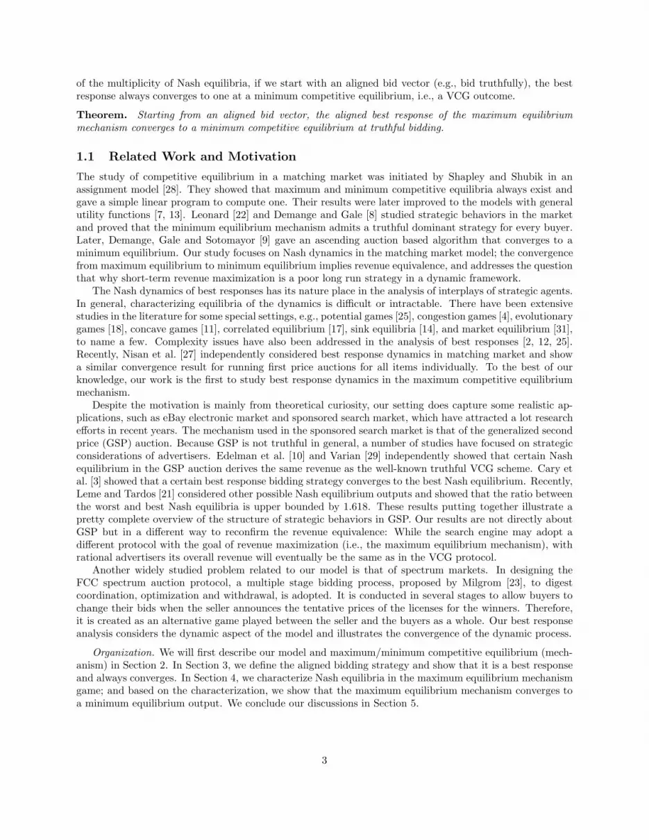
The above example further shows that best response strategies may not be unique: While i1 alwayswants to bid 10+ ǫ for j1, he can bid any value between 0 and 10 for j2 to constitute a best response. Whilethe bids for those items in which a buyer is not interested (i.e., j2 in the above example) will not affect theutility that the buyer obtains after his best response bidding, they do affect the overall convergence of thebest response dynamics, as the following example shows.
vi1j1 = 100
vi2j1 = 5
vi2j2 = 2i2
i1
j2
j1bi1j1 = 100
bi2j1 = 5
bi2j2 = 22
100
bi1j1 = 100
bi2j1 = 0
bi2j2 = ǫǫ
100
bi1j1 = ǫ
bi2j1 = 0
bi2j2 = ǫǫ
ǫbi1j1 = ǫ
bi2j1 = 2ǫ
bi2j2 = 00
2ǫ
bi1j1 = 3ǫ
bi2j1 = 2ǫ
bi2j2 = 00
3ǫ
bi1j1 = 3
bi2j1 = 3− ǫ
bi2j2 = 00
3
bi1j1 = 3
bi2j1 = 0
bi2j2 = ǫǫ
3
Figure 1: A best response that does not converge.
Example 3.1. (Non-convergence of a best response) There are two buyers i1, i2 and two items j1, j2,where vi1j1 = 100, vi1j2 = 0, vi2j1 = 5 and vi2j2 = 2. (There still are dummy buyers; we do not describe themexplicitly.) Consider the following specific best response strategy: Every buyer in the best response alwaysbids zero to those items that he is not interested in. Since vi1j2 = 0, we assume that i1 always bids zero toj2. The process in Figure 1 shows that the best response dynamics does not converge. (For all examples inthe paper, the black vertices on the left denote the buyers who change their bids in the best response, the solidlines denote allocations, and the numbers along with item vertices denote the maximum equilibrium prices.)
3.1 Best Response Strategy
Given the non-convergence of a specific best response shown in Example 3.1, one would ask if there areany best response strategies that always converge for any given instance. We consider the following biddingstrategy.
1When buyers report the same bids on some items, a certain tie-breaking rule should be specified to decide an equilibriumallocation. In the literature, ties are broken either by an oracle access to the true valuations or by a given fixed order ofbuyers [19, 20]. In our worst-case analysis framework, we actually do not need to specify a tie-breaking rule explicitly. Itessentially implies that (i) a buyer who changes his bid has the lowest priority in tie-breaking, and (ii) any buyer who bids zerocannot win the corresponding item at price zero due to the existence of dummy buyers (i.e., there is no free lunch).
2For any fixed bids of other buyers, the utility that a risk-averse buyer obtains in a best response is always within a distanceof ǫ to that in a best possible allocation that a risk-seeking buyer may obtain. Thus, the worst case analysis (i.e., with risk-aversebuyers) does provide a “safe” equilibrium allocation in which the corresponding utility is almost the same as the maximal.
7

Lemma 3.1. (Best response of losers) For any given bid vector b, let (p,x) = max-eq(b). Givenfixed bids of other buyers, consider any buyer i0 with xi0 = ∅; let di0 = maxj vi0j − pj.
• If di0 ≤ 0, a best response of i0 is to bid the same vector (bi0j)j.
• Otherwise, a best response of i0 is given by vector (b′i0j)j, where b′i0j = max{0, vi0j − di0 + ǫ}. Further,
the utility that i0 obtains after the best response bidding is either di0 or di0 − ǫ.3
Lemma 3.2. (Best response of winners) For any given bid vector b, let (p,x) = max-eq(b). Givenfixed bids of other buyers, consider any buyer i0 with xi0 6= ∅. Denote by b 6∋i0 the bid vector derived from b
where i0 changes his bid to 0 for all items. Let (q,y) = max-eq(b 6∋i0) and di0 = maxj vi0j − qj.
• If di0 ≤ 0 or ui0(p,x) = di0 , a best response of i0 is to bid the same vector (bi0j)j.
• Otherwise, a best response of i0 is given by vector (b′i0j)j, where b′i0j = max{0, vi0j − di0 + ǫ}. Further,
the utility that i0 obtains after the best response bidding is either di0 or di0 − ǫ.4
The best response (b′i0j)j defined in the above two lemmas has two remarkable properties: First, ifvi0j ≥ vi0j′ then b′i0j ≥ b′i0j′ ; second, if b
′ij , b
′ij′ > 0 then vi0j − b′i0j = vi0j′ − b′i0j′ . Hence, the best response
(b′i0j)j captures the preference of i0 over all items. In addition, given fixed bids of other buyers, the differencevi0j − b′i0j gives the maximal possible utility (up to a gap of ǫ) that i0 is able to obtain from item j.
We say a bid vector (bij)j aligned if for any bij , bij′ > 0, vij − bij = vij′ − bij′ . That is, (bij)j is derivedfrom (vij)j by moving the curve down in parallel capped at 0. It can be seen that the bid vectors definedin the above Lemma 3.1 and Lemma 3.2 are aligned. Hence, we will refer such bidding strategy by alignedbest response. In the following, unless stated otherwise, all best responses are aligned according to thesetwo lemmas. The following Figure 2 shows the convergence of Example 3.1 according to the aligned bestresponse when both buyers bid their true values initially (as in Figure 1).
bi1j1 = 100
bi2j1 = 5
bi2j2 = 22
100
bi1j1 = 100
bi2j1 = 3 + ǫ
bi2j2 = ǫǫ
100
bi1j1 = 3 + ǫ
bi2j1 = 3 + ǫ
bi2j2 = ǫǫ
3 + ǫ
Figure 2: Convergence of Example 3.1 by the aligned best response.
vi1j1 = 3
vi2j1 = 10
vi2j2 = 10
vi3j2 = 2i3
i2
i1
j2
j1
bi1j1 = 3
bi2j1 = 3
bi2j2 = 2
bi3j2 = 2
2
3
bi1j1 = 3
bi2j1 = 2 + ǫ
bi2j2 = 2 + ǫ
bi3j2 = 2
2 + ǫ
3
bi1j1 = 2 + ǫ
bi2j1 = 2 + ǫ
bi2j2 = 2 + ǫ
bi3j2 = 2
2 + ǫ
2 + ǫ
Figure 3: Non-monotonicity of the aligned best response.
3Note that if di0 > ǫ, then certainly i0 improves his utility through the best response bidding. If di0 = ǫ, however, it ispossible that i0 obtains the same utility di0 − ǫ = 0 = ui0 (p,x) after the best response bidding. For such a case, (b′i0j)j isstill a best response and we assume that i0 will continue to change his bid according to it. This assumption is without lossof generality as our focus is on the convergence of the best response strategy. Further, in practice, buyers usually do not havecomplete information about the market (e.g., bid vectors of others) and are unaware of the exact utility they will obtain ifchange their bids. Hence, continuing to bid the best response provides a safe strategy for the buyers to maximize their utilities.
4Similar to the discussions for Lemma 3.1, if ui0 (p,x) < di0 − ǫ, then i0 strictly improves his utility after the best responsebidding; if ui0 (p,x) = di0 − ǫ, it is possible that i0 obtains the same utility di0 − ǫ after the best response bidding. Again forsuch a case, (b′i0j)j is still a best response and we assume that i0 will continue change his bid according to it.
8

3.2 Properties of the Best Response
Example 1.1 shows that maximum equilibrium prices may not be monotone with respect to the submittedbid vectors. Such non-monotonicity still occurs even for the aligned best response of the winners defined inLemma 3.2. In the example of the Figure 3, when a winner i2 changes his bid, the price of j2 is increased from2 to 2 + ǫ in the maximum equilibrium. Hence, the maximum equilibrium prices may not be monotonicallydecreasing with respect to the aligned best responses of the winners.
However, as the following claim shows, we do have monotonicity for the maximum equilibrium pricesgiven a certain condition. This property is crucial in the analysis of convergence.
Lemma 3.3. When a loser makes a best response bidding (by Lemma 3.1), the maximum equilibrium priceswill not decrease. On the other hand, when a winner, who has already made at least one aligned best responsebidding, makes a best response bidding (by Lemma 3.2), the maximum equilibrium prices will not increase.
We have the following corollary.
Corollary 3.1. Given a bid vector b and (p,x) = max-eq(b), any loser i0 is willing to make a best responsebidding only if there is an item j such that vi0j > pj. For any winner i0 who has already made a best responsebidding, the following claims hold:
• i0 is willing to make a best response bidding b′ only if the price of item xi0 will decrease in max-eq(b 6∋i0)(defined in Lemma 3.2).
• Let (q,y) = max-eq(b 6∋i0) and (p′,x′) = max-eq(b′), then (p′,x) is a max-eq for b′ as well. Hence,we can assume without loss of generality that when i0 places a best response bidding, the allocationremains the same.
3.3 Convergence of the Best Response Dynamics
In this subsection we will show that the aligned best response defined in Lemma 3.1 and 3.2 always converges.In the rest of this subsection we will assume that all buyers have already made a best response bidding; thisassumption is without loss of generality since our goal is to prove convergence. Hence, the results establishedin the last subsection can be applied directly.
Proposition 3.1. Given a bid vector b and (p,x) = max-eq(b), assume that a winner i0 first makes abest response bidding.
• If next another winner i′0 makes a best response bidding, then i0 will not change his bid in the bestresponse.
• If next a loser i′0 makes a best response bidding, then as long as i0 is still a winner after i′0’s bid, hewill not change his bid in the best response.
Similar to Proposition 3.1, we have the following claim for the best response of losers.
Proposition 3.2. Given a bid vector b and (p,x) = max-eq(b), assume that a loser i0 first makes a bestresponse bidding and becomes a winner.
• If next another winner i′0 makes a best response bidding, then i0 will not change his bid in the bestresponse.
• If next another loser i′0 makes a best response bidding, then as long as i0 is still a winner after i′0’s bid,he will not change his bid in the best response.
The above two propositions imply the following corollary.
Corollary 3.2. Given a bid vector b and (p,x) = max-eq(b),
9

• if a winner i0 makes a best response bidding, then unless i0 becomes a loser (due to the best responsesof others), he will not change his bid in the best response;
• if a loser i0 makes a best response bidding and becomes a winner, then unless i0 becomes a loser again(due to the best responses of others), he will not change his bid in the best response.
We are now ready to prove our main theorem.
Theorem 3.1. In the maximum competitive equilibrium mechanism game, for any given initial bid vectorand any ordering of the buyers, the aligned best response defined in Lemma 3.1 and 3.2 always converges.
Proof. By Corollary 3.2, after all buyers have already made a best response bidding, only losers are willing tomake best responses to become a winner and winners are willing to make best responses only if they becomea loser. By Lemma 3.3, the prices will be monotonically non-decreasing when losers make best responses.Hence, the process eventually terminates.
The above theorem only says that the aligned best response is guaranteed to converge in finite steps;indeed it may take a polynomial of maxij vij/ǫ steps to converge. This is true even for the simplest settingwith one item and two buyers of the same value v1 = v2: The two buyers with initial bids zero keepincreasing their bids by 2ǫ one by one to beat each other until the price reaches to v1 = v2. However, in mostapplications like advertising markets, the value of maxij vij is rather small. Further, to guarantee efficientconvergence, we may set ǫ to be sufficiently large so that the rally between the winners and losers is fast(e.g., in most ascending auctions, the minimum increment of a bid is scaled according to the expected valueof maxij vij).
4 Characterization of Nash Dynamics: From max-eq to min-eq
Theorem 3.1 in the previous section shows that the aligned best response always converges for any giveninitial bid vector. However, it does not answer the questions of at which condition(s) the dynamics of thebest response stops (i.e., reaches to a stable state), and how the stable state looks like. We will answer thesequestions in this section.
Theorem 4.1. For any Nash equilibrium bid vector b of the max-eq mechanism, let (p,x) = min-eq(b)and (q,y) = max-eq(b). Then for any item j, we have either pj = qj or pj + ǫ = qj. That is, the max-eqand min-eq price vectors differ by at most ǫ, i.e., max-eq(b) ≈ min-eq(b).
The above characterizations apply to all Nash equilibria in the max-eq mechanism, and gives a necessarycondition that when a bid vector forms a Nash equilibrium. Note that the other direction of the claim doesnot hold. For example, there are one item and two buyers with the same true value v1 = v2 = 10. In thebid vector b with b1 = b2 = 5, we have max-eq(b) = min-eq(b). However, b is not a Nash equilibrium asthe loser in the max-eq(b) can increase his bid to win the item.
In general, there can be multiple Nash equilibria for a given market. To compare different Nash equilibria,we use a universal benchmark — the solution given by the truthful min-eq mechanism, i.e., (p∗,x∗) =min-eq(v), where v is the true valuation vector. This is equivalent to the outcome of the second priceauction in single item markets and the VCG mechanism for the general multi-item markets. In Appendix D,we give two examples to show that, for a given Nash equilibrium b with (p,x) = max-eq(b), there couldbe no fixed relation between the price vectors p and p∗, i.e., it can be either p ≫ p∗ or p ≪ p∗. This is aremarkable difference between single item and multi-item markets — in the former we always have p ≈ p∗
(i.e., ||p− p∗|| ≤ ǫ).However, if we initially start with an aligned bid vector for all buyers (e.g., bid truthfully), then there is a
strong connection between the max-eq price vector at a converged Nash equilibrium and (p∗,x∗): The twoprice vectors are “almost” identical, up to a gap of ǫ. We summarize our results in the following theorem.
10

Theorem 4.2. For any Nash equilibrium bid vector b converged from the aligned best response, startingfrom an aligned bid vector for all buyers, let (p,x) = max-eq(b) and (p∗,x∗) = min-eq(v), where v = (vij)is the true valuation vector. Then we have
• either pj = p∗j or pj = p∗j + ǫ for all items;
• max-eq(b) ≈ min-eq(b) ≈ min-eq(v).
We comment that if we start with an arbitrary bid vector, as long as all buyers bid at least one alignedbest response in the dynamics, the convergence result from max-eq to min-eq still holds. In particular, thisincludes the case when all buyers bid very low at the beginning. In addition, for any given bid vector b, ifthe max-eq mechanism outputs max-eq(b) = min-eq(v), it is not necessary that b is a Nash equilibrium.For example, it is possible that the bids of losers are quite small and therefore winners still want to decreasetheir bids to pay less.
Finally, we characterize allocations at all Nash equilibria. We say an allocation x efficient if∑
i vixiis
maximized, i.e., social welfare is maximized. It is well-known that all allocations in competitive equilibriaare efficient at truthful bidding. This can be easily generalized to say that for any given bid vector b,any equilibrium allocation x maximizes
∑i bixi
. We have the following result, which says that any Nashequilibrium converged from the aligned best response actually maximizes the real social welfare with respectto v.
Theorem 4.3. For any Nash equilibrium bid vector b of the max-eq mechanism converged from the alignedbest response (starting from an arbitrary bid vector), let (p,x) = max-eq(b). Then x is an efficient allocationthat maximizes social welfare.
We note that the above claim does not hold for general Nash equilibria. For example, buyers i1 and i2are interested in item j1 at values vi1j1 = v and vi2j1 = v + ǫ. Then allocating the item to i1 at price v is aNash equilibrium for the bid vector bi1j1 = bi2j1 = v (since the second buyer i2 still obtains a non-positiveutility even if he can win the item at a higher bid). This allocation does not maximize social welfare, andthe example can be easily generalized to arbitrary number of items with large deficiency. In the aligned bestresponse bidding, however, i2 will continue to bid v + ǫ to win the item by Lemma 3.1, which leads to anefficient allocation.
5 Concluding Remarks
In this paper, we analyze the dynamics of best responses of the maximum competitive equilibrium mechanismin a matching market. While a best response strategy may not necessarily converge, we show that a specificbidding strategy, aligned best response, always converges to a Nash equilibrium. The outcome at such a Nashequilibrium is actually a minimum equilibrium given truthful bidding if we start with an aligned bid vector.In other words, our results show that maximum equilibrium converges to minimum equilibrium, which isa reminiscence of the convergence of dynamic bidding from first price auction to second price auction in asingle item market.
In our discussions, we assume that all buyers have complete information for the market, including, say,submitted bid vectors of others, market prices and their corresponding allocation. We note that the firstone, submitted bids of other buyers, in not necessary in the dynamics: The best response of losers defined inLemma 3.1 applies automatically, and the best response of winners defined in Lemma 3.2 can be implementedby a two-step strategy without requiring extra information in the market.
11

References
[1] G. Aggarwal, A. Goel, R. Motwani, Truthful Auctions for Pricing Search Keywords, EC 2006, 1-7.
[2] E. Ben-Porath, The Complexity of Computing a Best, Response Automaton in Repeated Games with Mixed
Strategies, Games and Economic Behavior, V.2, 1-12, 1990.
[3] M. Cary, A. Das, B. Edelman, I. Giotis, K. Heimerl, A. Karlin, C. Mathieu, M. Schwarz, On Best-Response
Bidding in GSP Auctions, EC 2007, 262-271.
[4] S. Chien, A. Sinclair, Convergence to Approximate Nash Equilibrium in Congestion Games, Games and EconomicBehavior, 2009.
[5] E. H. Clarke, Multipart Pricing of Public Goods, Public Choice, V.11, 17-33, 1971.
[6] P. Cramton, The FCC Spectrum Auctions: An Early Assessment, Journal of Economics and ManagementStrategy, V.6(3), 431-495, 1997.
[7] V. Crawford, E. Knoer, Job Matching with Heterogeneous Firms and Workers, Econometrica, V.49(2), 437-450,1981.
[8] G. Demange, D. Gale, The Strategy of Two-Sided Matching Markets, Econometrica, V.53, 873-888, 1985.
[9] G. Demange, D. Gale, M. Sotomayor, Multi-Item Auctions, Journal of Political Economy, V.94(4), 863-872,1986.
[10] B. Edelman, M. Ostrovsky, M. Schwarz, Internet Advertising and the Generalized Second-Price Auction, Amer-ican Economic Review, 97(1), 242-259, 2007.
[11] E. Even-Dar, Y. Mansour, U. Nadav, On the Convergence of Regret Minimization Dynamics in Concave Games,STOC 2009, 523-532.
[12] A. Fabrikant, C. H. Papadimitriou, The Complexity of Game Dynamics: BGP Oscillations, Sink Equilibria, and
Beyond, SODA 2008, 844-853.
[13] D. Gale, Equilibrium in a Discrete Exchange Economy with Money, International Journal of Game Theory, V.13,61-64, 1984.
[14] M. Goemans, V. Mirrokni, A. Vetta, Sink Equilibria and Convergence, FOCS 2005, 142-154.
[15] T. Groves, Incentives in Teams, Econometrica, V.41, 617-631, 1973.
[16] F. Gul, E. Stacchetti, Walrasian Equilibrium with Gross Substitutes, Journal of Economic Theory, V.87, 95-124,1999.
[17] S. Hart, A. Mas-Colell, A Simple Adaptive Procedure Leading to Correlated Equilibrium, Econometrica, V.68,1127-1150, 2000.
[18] J. Hofbauer, K. Sigmund, Evolutionary Game Dynamics, Bulletin of the American Mathematical Society, V.40,479-519, 2003.
[19] N. Immorlica, D. Karger, E. Nikolova, R. Sami, First-Price Path Auctions, EC 2005, 203-212.
[20] A. R. Karlin, D. Kempe, T. Tamir, Beyond VCG: Frugality of Truthful Mechanisms, FOCS 2005, 615-626.
[21] R. P. Leme, E. Tardos, Pure and Bayes-Nash Price of Anarchy for Generalized Second Price Auction, FOCS2010.
[22] H. B. Leonard, Elicitation of Honest Preferences for the Assignment of Individuals to Positions, Journal ofPolitical Economy, V.91, 461479, 1983.
[23] P. Milgrom, Putting Auction Theory to Work, Cambridge University Press, 2004.
12

[24] V. Mirrokni, A. Skopalik, On the Complexity of Nash Dynamics and Sink Equilibria, EC 2009, 1-10.
[25] D. Monderer, L. Shapley, Potential Games, Games and Economic Behavior, V.14(1), 124-143, 1996.
[26] R. Myerson, Optimal Auction Design, Mathematics of Operations Research, V.6, 58-73, 1981.
[27] N. Nisan, M. Schapira, G. Valiant, and A. Zoha, Best Response Auctions, EC 2011.
[28] L. Shapley, M. Shubik, The Assignment Game I: The Core, International Journal of Game Theory, V.1(1),111-130, 1971.
[29] H. Varian, Position Auctions, International Journal of Industrial Organization, V.6, 1163-1178, 2007.
[30] W. Vickrey, Counterspeculation, Auctions, and Competitive Sealed Tenders, Journal of Finance, V.16, 8-37,1961.
[31] F. Wu, L. Zhang, Proportional Response Dynamics Leads to Market Equilibrium, STOC 2007, 354-363.
A Proof of Theorem 2.1
Lemma A.1. Let (p,x) and (p′,x′) be any two equilibria for the given bid vector b. Let T = {j | pj < p′j}and S = {i | x′
i ∈ T } be the subset of buyers who win items in T in the equilibrium (p′,x′). Then all buyersin S win all items in T in the equilibrium (p,x) as well. In particular, this implies that if j is allocated toa dummy buyer in (p,x) (i.e., essentially no one wins j), then its price is zero in all equilibria.
Proof. Note that since p′j > pj ≥ 0 for any j ∈ T , all items in T must be sold out in equilibrium (p′,x′);hence, |S| = |T | and all buyers in S win all items in T in (p′,x′). Consider any buyer i ∈ S, let j′ = x′
i ∈ T .For any item j /∈ T , since pj ≥ p′j , we have
bij′ − pj′ > bij′ − p′j′ ≥ bij − p′j ≥ bij − pj
where the second inequality follows from the fact that (x′,p′) is an equilibrium. Hence, buyer i always strictlyprefers item j′ to all other items not in T at price vector p, which implies that his allocation xi ∈ T .
Proof of Theorem 2.1. By the rule of increasing prices, since the initial (p,x) is an equilibrium, all buyersare always satisfied with their respective allocations in the course of the algorithm. Further, it can be seenthat any item that is allocated to a dummy buyer (i.e., it has initial price pj = 0) will never have its priceincreased. Hence, the final output (q,x) is an equilibrium as well.
Assume that (x∗,q∗) is a max-eq for the given bid vector b; we know that qj ≤ q∗j for all items. LetT = {j | qj < q∗j } and S = {i | x∗
i ∈ T } be the subset of buyers who win items in T in the max-eqequilibrium. By Lemma A.1, we know that all buyers in S win all items in T in equilibrium (q,x) as well.Assume that T 6= ∅; and consider any j1 ∈ T and the subgraph Gmax
j1(b,q,x) reachable from j1 in the
demand graph of the final output (q,x).We claim that all items in Gmax
j1are in T . Otherwise, consider an item jℓ ∈ Gmax
j1\ T and the max-
alternating path (j1, i1, j2, i2, . . . , iℓ−1, jℓ) defining jℓ to be in Gmaxj1
. Assume without loss of generality thatjℓ is the first item on the path which is not in T , i.e., jℓ−1 ∈ T and jℓ /∈ T . since jℓ−1 = xiℓ−1 ∈ T , byLemma A.1, we have j∗ , x∗
iℓ−1∈ T . Hence,
biℓ−1jℓ − q∗jℓ ≥ biℓ−1jℓ − qjℓ
= biℓ−1jℓ−1 − qjℓ−1
≥ biℓ−1j∗ − qj∗
> biℓ−1j∗ − q∗j∗
which contradicts to the fact that iℓ−1 obtains his utility-maximized item in the max-eq.Since all items in Gmax
j1have their prices increased, again by Lemma A.1, all items in Gmax
j1are sold out.
Therefore, at the end of the algorithm when reaching to (q,x), we should still be able to increase prices foritems in Gmax
j1, which is a contradiction. That is, T = ∅ and (q,x) is a max-eq. �
13

B Proofs in Section 3
B.1 Proof of Lemma 3.1
Proof. Given fixed bids of other buyers, consider any bid vector (b∗i0j)j of buyer i0. Denote the resultingbid vector by b∗, and let (p∗,x∗) = max-eq(b∗). A basic observation is that no matter what bid that i0submits, everyone other than i0 is still happy with the original equilibrium (p,x). Hence, if b∗i0j ≤ pj forany j, then (p,x) is still a max-eq for b∗. Otherwise, let j1 ∈ argmaxj{b
∗i0j
− pj}. Consider subgraphGmax
j1(b,p,x) and its critical max-alternating path (j1, i1, j2, i2, . . . , jℓ, iℓ) with respect to x, where xik = jk
for k = 1, . . . , ℓ−1 and the pair iℓ and jℓ is the reason that pj1 cannot be increased in (p,x) by the algorithm(i.e., biℓjℓ = pjℓ). Consider reallocating each jk to ik−1 for k = 2, . . . , ℓ. By the definition of max-alternatingpath, we know that all these buyers are still happy with their new allocations. Further, we reallocate j1 toi0; then i0 obtains his utility-maximized item at price p under bid vector b∗. This new allocation, togetherwith the price vector p, constitutes an equilibrium. In both cases, p is an equilibrium price vector under bidvector b∗. Hence, the price of every item in max-eq(b∗) is larger than or equal to pj , i.e., p
∗j ≥ pj .
We next analyze the best response of i0 defined in the statement of the claim. If vi0j ≤ pj for any j, theni0 cannot get a positive utility from any item at price vector p, as well as p∗. Hence, bidding the original(losing) price vector is a best response strategy. It suffices to consider there is an item j such that vi0j > pjand the best response strategy (b′i0j)j described in the second part of the statement (denoted by b′).
Let T = {j | vi0j − pj = di0}; by the assumption, T 6= ∅. It can be seen that for any j ∈ T , b′ij − pj = ǫ;and any j /∈ T , b′ij − pj ≤ vi0j − di0 + ǫ− pj < di0 − di0 + ǫ = ǫ, i.e., b′ij − pj ≤ 0. That is, given bid vector b′
and price vector p, i0 always desires those items in T . Consider any item j0 ∈ T , by the same reassignmentargument described above, we can reallocate j0 to i0, as well as a few other reallocations through a criticalmax-alternating path, to derive an equilibrium (p,x′), where x′ is the corresponding new allocation. Notethat (p,x′) may not be a max-eq. Consider subgraph Gmax
j0(b′,p,x′); we ask whether pj0 can be increased
further by the algorithm Alg-max-eq to get a max-eq.If the answer is ‘no’, then (p,x′) is indeed a max-eq under bid vector b′ (it can be shown that the price
of any other item cannot be increased as well), and the utility that i0 obtains satisfies
ui0(p,x′) = vi0j0 − pj0 = di0
= maxj
vi0j − pj ≥ maxj
vi0j − p∗j ≥ ui0(p∗,x∗)
If the answer is ‘yes’, then we can increase prices of all items in Gmaxj0
(b′,p,x′) by ǫ, which gives anequilibrium (p′,x′), where p′j = pj + ǫ if j ∈ Gmax
j0(b′,p,x′) and p′j = pj otherwise. Further, (p′,x′) is a
max-eq under bid vector b′ since the price of j0 is tight with the bid of i0, i.e., b′i0j0
= p′j0 (again, prices ofother items cannot be increased). Hence, the utility that i0 obtains is
ui0(p′,x′) = vi0j0 − p′j0 = vi0j0 − pj0 − ǫ = di0 − ǫ
Next we consider the utility that i0 obtains in the equilibrium (p∗,x∗) with bid vector b∗. Note that allother buyers bid the same values in b,b′ and b∗. Let j1 , x∗
i0; then
ui0(p∗,x∗) = vi0j1 − p∗j1 ≤ vi0j1 − pj1 ≤ di0
If one of the above inequalities is strict, then ui0(p∗,x∗) < di0 . That is, ui0(p
∗,x∗) ≤ di0 − ǫ = ui0(p′,x′),
which implies that b′ is a best response strategy. It remains to consider the case when all inequalities aretight, i.e., ui0(p
∗,x∗) = di0 and p∗j1 = pj1 ; in this case, we have j1 ∈ T . Consider the following two casesregarding the relation between j0 and j1.
• If j0 = j1, consider the subgraph Gmaxj1
(b∗,p∗,x∗). Since the price of j1 cannot be increased, there isa critical max-alternating path inside P = (j1, i1 = i0, j2, i2, . . . , jℓ, iℓ) where x∗
ik= jk and b∗iℓjℓ = p∗jℓ .
Sinceb∗i0j2 − p∗j2 = b∗i0j1 − p∗j1 = b∗i0j1 − pj1
14

we know that j2 ∈ T and p∗j2 = pj2 (otherwise, vi0j2 −p∗j2 < di0 , then in the worst allocation the utilityof i0 is less than di0). We claim that all items in P have p∗j = pj . Otherwise, consider the first item jkwhere p∗jk > pjk . Note that k ≥ 3; then we have
b′ik−1jk−1− pjk−1
= b∗ik−1jk−1− p∗jk−1
= b∗ik−1jk− p∗jk
< b∗ik−1jk− pjk
= b′ik−1jk− pjk
Hence, x′ik−1
∈ T ∗ , {j | p∗j > pj} and x∗ik−1
= jk−1 /∈ T ∗. This implies that there must be a buyer i
such that x′i /∈ T ∗ and x∗
i ∈ T ∗, which is impossible since i does not get his utility-maximized item in(p,x′). Therefore, essentially P defines a critical max-alternating path in Gmax
j0(b′,p,x′).
• If j0 6= j1, starting from P ′ = (j0, i0, j1), we expand the path P ′ through the following rule: if thecurrent last edge is (ik, jk+1), expand (jk+1, ik+1) if x′
ik+1= jk+1; if the current last edge is (jk, ik),
expand (ik, jk+1) if x∗ik
= jk+1. The process stops when there is no more item or buyer to expand;denote the final path by P ′ = (j0, i0, j1, i
′1, j
′2, i
′2, . . . , jℓ, i
′ℓ). Note that edges in P ′ are in x′ and x∗
alternatively. Further, since i′1 wins j1 in x′ and j′2 in x∗, plus the fact that p∗j1 = pj1 , we have p∗j′2
= pj′2;
then since i′2 wins j′2 in x′ and j′3 in x∗, we have p∗j′3
= pj′3; the argument inductively implies that for
every item j ∈ P ′, p∗j = pj . At the end of path P ′, i′ℓ does not win any item in x∗, which implies thatb′i′
ℓj′ℓ
= pj′ℓ. If we consider path P ′ in Gmax
j0(b′,p,x′), the above arguments show that it is actually a
critical max-alternating path.
Hence, in both cases we cannot increase price pj0 in the equilibrium (p,x′), which contradicts to our as-sumption that the answer is ‘yes’.
B.2 Proof of Lemma 3.2
Proof. Given fixed bids of other buyers, consider any bid vector (b∗i0j)j of buyer i0. Denote the resulting bidvector by b∗, and let (p∗,x∗) = max-eq(b∗). Consider the two equilibria (q,y) and (p∗,x∗) in the followingvirtual scenario: i0 first bids 0 and loses in the max-eq (q,y) and then bids according to b∗ yielding a newmax-eq (p∗,x∗). By a similar argument as the proof of the above lemma, we know that qj ≤ p∗j for allitems. In particular, the argument applies to the case when b∗ = b, hence qj ≤ pj .
Since the bid of any buyer is always less than or equal to his true value, we have
ui0(p,x) = vi0xi0− pxi0
≥ bi0xi0− pxi0
≥ 0
If ui0(p,x) = di0 , then certainly i0 cannot obtain more utility when bidding b∗ since
ui0(p∗,x∗) = vi0x∗
i0
− p∗x∗
i0
≤ vi0x∗
i0
− qx∗
i0
≤ di0 = ui0(p,x)
If di0 ≤ 0, thenvi0xi0
− pxi0≤ vi0xi0
− qxi0≤ 0
andui0(p
∗,x∗) = vi0x∗
i0
− p∗x∗
i0
≤ vi0x∗
i0
− qx∗
i0
≤ 0
Hence, ui0(p,x) = 0 ≥ ui0(p∗,x∗), which implies that bidding the original vector (bi0j)j is a best response
strategy.It remains to consider di0 > ui0(p,x) ≥ 0 and analyze the best response (b′i0j)j , denote by b′, defined
in the statement of the claim. Consider a virtual scenario where i0 first bids 0 and loses in the equilibrium(q,y). By the above Lemma 3.1 for loser’s best response, we know that b′ is a best response strategy for i0in the virtual scenario and ui0(b
′) ≥ di0 − ǫ ≥ ui0(p,x). Since bidding according to b∗ is a specific strategyfor i0, we have ui0(b
′) ≥ ui0(p∗,x∗). These two inequalities together imply that bidding according to b′ is
a best response strategy for i0.
15

B.3 Proof of Lemma 3.3
Proof. The first part of the claim follows directly from the proof of Lemma 3.1, thus we will only prove thesecond part. Consider bid vector b and equilibrium (p,x) = max-eq(b), bid vector b 6∋i0 (derived from b
where a winner i0 bids 0 for all items) and equilibrium (q,y) = max-eq(b 6∋i0), and best response b′, alldefined in the statement of Lemma 3.2. If i0 does not change his bid, then the maximum equilibrium pricesremain the same. Hence, in the following we assume that i0 changes his bid according to b′ and analyze therelation between p and p′, where (p′,x′) = max-eq(b′). What we need to show is that p′ ≤ p.
By the proof of Lemma 3.2, we know that qj ≤ pj for all items. If q = p, i.e., qj = pj for all items, letj∗ = argmaxj vij − qj . Note that di0 = vi0j∗ − qj∗ > 0. Since (p,x) is an equilibrium with respect to b, wehave bi0xi0
− pxi0≥ bi0j∗ − pj∗ and bi0xi0
6= 0. Since i0 has already made a best response bidding (either asa loser or a winner), his bids for different items are aligned, i.e., vi0xi0
− bi0xi0≥ vi0j∗ − bi0j∗ . Thus,
ui0(p,x) = vi0xi0− pxi0
≥ vi0j∗ − pj∗ = vi0j∗ − qj∗ = di0
Hence, i0 already obtains his maximally possible utility and will not change his bid. In the following, weassume q ≤ p and there is an item such that qj < pj .
Let T = {j | qj < pj} and S = {i | xi ∈ T } be the set of buyers who win items in T in (p,x). Weclaim that i0 ∈ S. Otherwise, all buyers in S win all items in T in (q,y) as well with positive utilities andthey strictly prefer their corresponding allocations to those items that are not in T . Hence, we can increasethe prices of all items in T by ǫ to derive another equilibrium; this contradicts to the fact that (q,y) is amax-eq. Therefore, there is exactly one buyer i∗ /∈ S who wins an item in T in (q,y) given bid vector b 6∋i0 ,i.e., yi∗ ∈ T . Next when i0 changes his bid vector according to b′, by the proof of Lemma 3.1, the newallocation vector x′, together with the given price vector q, constitutes an equilibrium. Let j0 = x′
i0; since
vi0j0 − qj0 = maxj
vi0j − qj = di0
> ui0(p,x)
= vi0xi0− pxi0
≥ vi0j0 − pj0
we must have j0 ∈ T . That is, when i0 “joins the market again” from b 6∋i0 to b′, he grabs an item in T“again”. Since every buyer in S \ {i0} obtains a positive utility for his corresponding allocation in T in(q,y) and strictly prefers it to those items that are not in T , he has to win an item in T in (q,x′). Hence,the only buyer who is kicked out of winning an item in T is i∗. That is, buyers in S “again” win all itemsin T . Finally, without loss of generality, we can assume that in x′ all items that are not in T have thesame allocations as x; this still keeps an equilibrium and will not affect the computation of the maximumequilibrium price vector. Our argument above can be summarized as below:
bid vector equilibrium winners for items in Tb max-eq (p,x) S \ {i0} ∪ {i0}b 6∋i0 max-eq (q,y) S \ {i0} ∪ {i∗}
(q,x′)b′
max-eq (p′,x′)S \ {i0} ∪ {i0}
Finally we consider running the algorithm Alg-max-eq on equilibrium (q,x′) to derive the maximumequilibrium (p′,x′). By the proof of Lemma 3.1, we have either p′j = qj or p′j = qj + ǫ. To the end ofproving p′j ≤ pj , it remains to show that it is impossible that p′j = qj + ǫ = pj + ǫ for all items; assumeotherwise that there is such an item jℓ (this implies that jℓ /∈ T ). Then again by the proof of Lemma 3.1,the price of jℓ is increased (from q to p′) through a max-alternating path P = (j0, i0, j1, i1, . . . , jℓ−1, iℓ−1, jℓ)in the subgraph Gmax
j0(b′,q,x′). That is, for k = 0, 1, . . . , ℓ − 1, x′
ik= jk and vikjk − qjk = vikjk+1
− qjk+1.
Consider subgraph Gmaxjℓ
(b,p,x), since (p,x) = max-eq(b), we cannot increase pjℓ and there is a criticalmax-alternating path P ′ in Gmax
jℓ(b,p,x). Further, it can be seen that all items in P ′ are not in T (since
every buyer in P ′ strictly prefers the corresponding allocation in x to those items in T at price vector p).
16

Since all items that are not in T have the same allocations in x and x′, we can expand path P through P ′,which gives a critical max-alternating path in Gmax
j0(b′,q,x′). Therefore, we cannot increase the price of
any item in P ∪ P ′, including jℓ. This contradicts to our assumption that p′jℓ = qjℓ + ǫ; hence the lemmafollows.
B.4 Proof of Corollary 3.1
Proof. The claims for best responses follow directly from Lemma 3.1 and 3.2, and the proof of Lemma 3.3.For the last claim, note that if (q,x) is an equilibrium for b′, then by the algorithm Alg-max-eq to increaseprices to derive the maximum equilibrium price vector p′, (p′,x) is a max-eq for b′. Recall in the proof ofLemma 3.3, (q,x′) is an equilibrium of b′ and all items that are not in T have the same allocations as x,where T = {j | qj < pj}. Thus, it remains to show that all items in T have the same allocations in x andx′. Since all items in T are allocated to the same subset of buyers S in both x and x′, for any buyer i ∈ S,we have
ui(p,x) = bixi− pxi
≥ bix′
i− px′
i
ui(q,x′) = bix′
i− qx′
i≥ bixi
− qxi, if i 6= i0
and
ui0(q,x′) = b′i0x′
i0
− qx′
i0
≥ b′i0xi0− qxi0
=⇒ bi0x′
i0
− qx′
i0
≥ bi0xi0− qxi0
(The last inequality is because of the following argument: Assume that b′i0x
′
i0
= bi0x′
i0
− δ. Since i0 has
already made a best response bidding, his bid vector over different items has already been aligned. By thebest responses defined in Lemma 3.1 and 3.2, we have vi0x′
i0
−bi0x′
i0
≤ vi0x′
i0
−b′i0x′
i0
. Hence δ ≥ 0 and b′i0xi0=
max{0, bi0xi0− δ} ≥ bi0xi0
− δ. Therefore, bi0x′
i0
− qx′
i0
= δ+ b′i0x′
i0
− qx′
i0
≥ δ+ b′i0xi0− qxi0
≥ bi0xi0− qxi0
.)
If items in T are allocated in different ways in x and x′, then there are T ′ ⊆ T and S′ ⊆ S such that itemsin T ′ are allocated to buyers in S′ in x and x′ which forms an augmenting path. Adding the above twoinequalities (regarding ui(p,x) and ui(q,x
′)) for all buyers in S′ gives∑
j∈T ′ pj+qj ≥∑
j∈T ′ pj+qj . Hence,all inequalities are tight, which implies that every buyer gets the same utility from xi and x′
i. Therefore, wecan change the allocation of items in T ′ according to x, which still gives an equilibrium.
B.5 Proof of Proposition 3.1
Proof. Assume that (q,y) = max-eq(b 6∋i0) and (p′,x) = max-eq(b′), where b′ is the resulting bid vectorafter i0 makes his best response bidding (by Corollary 3.1, we can assume that the equilibrium allocation isthe same for b and b′). Further, by the proof of Corollary 3.1, we know that (q,x) is an equilibrium for b′.In the two allocations x and y, consider the following alternating path:
P = (i0, j0 = xi0 , i1, j1, . . . , iℓ, jℓ, iℓ+1)
where ik wins jk in x and ik+1 wins jk in y, and xiℓ+1= ∅ (this implies, in particular, biℓ+1jℓ = qjℓ). Further,
we havebik+1jk − qjk = bik+1jk+1
− qjk+1, for k = 0, . . . , ℓ
We will analyze the relation between q and the price vector after i′0 makes his best response bidding to showthe desired result.
• First consider the next best response is made by another winner i′0. After i′0 makes his best responsebidding denote the resulting bid vector by b′′), by Corollary 3.1, we know that all winners have thesame allocations x. Further, the above set of equations still holds for all buyers in P for b′′. This is
17
because, if i′0 is one of them, say ik+1 = i′0, then both bik+1jk and bik+1jk+1are reduced by the same
amount to derive b′′ik+1jkand b′′ik+1jk+1
; so we still have b′′ik+1jk− qjk = b′′ik+1jk+1
− qjk+1. Hence, the
price of any item j in path P , as well as those that give the maximal utility to i0, cannot be smallerthan qj in max-eq(b′′) (otherwise, iℓ+1 has to be a winner).
Therefore, when i0 bids zero for all items after i′0 makes his best response bidding, the price of itemj0 cannot be smaller than qj0 in a max-eq(b′′
6∋i0) as reallocating items according to P where iℓ+1
becomes a winner gives an equilibrium allocation. By Corollary 3.1, which says that every winnerobtains the same item after his best response bidding, we know that the best response of i0 is to bidthe same vector, i.e., do not change his bid.
• Next consider the next best response is made by a loser i′0; let b′′ be the resulting bid vector. By the
proof of Lemma 3.1, let (p′,x′) be an equilibrium of b′′, where p′ is the maximum equilibrium price ofb′ defined above and x′ is derived from x (the allocation before i′0’s bid) through an alternating path:
P ′ = (i′0, j′1, i
′1, . . . , j
′r, i
′r)
where i′k wins j′k in x and i′k wins j′k+1 in x′, and i′r does not win in x′. (Note that to derive a max-eqfor b′′, we still need to verify if the price of j′1 can be increased in the subgraph Gmax
j′1
(b′′,p′,x′).)
Assume that i0 is still a winner after i′0’s bid; note that the item that i0 wins in x′ can be either theone defined above according to P ′ or the same item j0 = xi0 . Next we consider the setting when i0bids zero for all items, i.e., b′′
6∋i0 , for the two possibilities respectively.
If it is the former, i.e., i′k = i0, j′k = j0 and x′
i0= j′k+1, then the price of j′k and j′k+1 cannot be smaller
than p′j′k
(which is at least qj′k) and p′
j′k+1
(which is at least qj′k+1
) respectively in a max-eq(b′′6∋i0)
as we are able to reallocate items j′k+1, . . . , j′r back to i′k+1, . . . , i
′r, respectively, where j′r becomes a
winner. Since di0 defined in Lemma 3.2 will not increase, the best response of i0 is to bid the samevector, i.e., do not change his bid.
If it is the latter, i.e., i0 wins the same item j0 in x and x′, we claim that the price of j0 cannot besmaller than qj0 in a max-eq(b′′
6∋i0). This is because: (i) We can reallocate items according to P suchthat iℓ+1 becomes a winner. (ii) If any item in P ′ appears in P or i′0 = iℓ+1 (i.e., i′0 is the last buyeron path P ), similar to the above arguments, we can reallocate items according P and P ′ such that i′rbecomes a winner. (Note that for the last case i′0 = iℓ+1, since bi′
0jℓ = biℓ+1jℓ = qjℓ and the bids of i′0
have already been aligned, jℓ will give the maximal utility for i0 when its price is qjℓ .)
B.6 Proof of Proposition 3.2
Proof. An equivalent way to consider the best response of i0 is that he first bids 0 for all items (which yieldsthe same max-eq (p,x)), then bids according to the best response of winners defined in Lemma 3.2. Thenwe can apply the same argument as Proposition 3.1 to get the desired result.
B.7 Proof of Corollary 3.2
Proof. The proof of the claim is by induction on the process that buyers make the best response bidding.For every such best response bidding, we use the same proof in the above Proposition 3.1 and 3.2 to get thedesired result.
C Proofs in Section 4
To prove our results, we need the following definition, which is similar to max-alternating path.
18

Definition C.1 (min-alternating path). Given any equilibrium (p,x) of a given bid b, let G = G(b,p)be its demand graph. For any item j, a path (j = j1, i1, j2, i2, . . . , jℓ, (iℓ)) in G is called a min-alternatingpath if edges are not in and in the allocation x alternatively, i.e., xik = jk+1 for all possible k. Denoteby Gmin
j (b,p,x) (or simply Gminj when the parameters are clear from the context) the subgraph of G(b,p)
(containing both buyers and items including j itself) reachable from j through min-alternating paths withrespect to x. A min-alternating path (j = j1, i1, j2, i2, . . . , jℓ, iℓ) in Gmin
j (b,p,x) is called critical if xiℓ = ∅and biℓjℓ = pjℓ .
Note that the major difference between max and min-alternating paths is that in the former, edges inthe path are in and not in the allocation x alternatively; whereas in the latter, edges in the path are not inand in x alternatively. Similar to Corollary 2.1, we have the following claim. (The last pair jℓ and (iℓ) ina critical min-alternating path is the exact reason that why the price pj cannot be decreased further, sinceotherwise iℓ will have to be a winner and items are over-demanded.)
Corollary C.1. Given any bid vector b and (p,x) = min-eq(b), for any item j, there is a critical min-alternating path in Gmin
j (b,p,x).
C.1 Proof of Theorem 4.1
Proof. By the definition of (p,x) and (q,y), we have p ≤ q. Let T = {j | pj + ǫ < qj} and S = {i | yi ∈ T },i.e., S is the subset of buyers that win items in T in the max-eq (q,y). Then for any j /∈ T , either pj = qjor pj + ǫ = qj . Assume that T 6= ∅; similar to the proof of Lemma A.1, we know that all buyers in S stillwin items in T in the min-eq (p,x).
Consider any i0 ∈ S and let j0 = yi0 ∈ T . Consider a bid vector (b′i0j)j where b′i0j0 = qj0 − ǫ and b′i0j = 0for any j 6= j0; denote the resulting bid vector by b′ (where the bids of all other buyers remain the same).Consider a tuple (q′,y′), where q′j = qj − ǫ if j ∈ T and q′j = qj if j /∈ T , and y′i = yi if i ∈ S and y′i = xi ifi /∈ S. It can be seen that (q′,y′) is an equilibrium for b′. Note that b′i0j0 = qj0 − ǫ = q′j0 ; thus, i0 cannotobtain j0 if its price q′j0 is increased any further.
Let (q∗,y∗) = max-eq(b′); note that q′ ≤ q∗. We claim that i0 still wins j0 at price q∗j0
= q′j0 in (q∗,y∗).(This fact implies that i0 obtains more utility from j0 by paying ǫ less when bidding (b′i0j); thus max-eq(q,y) is not a Nash equilibrium.) Assume otherwise, then i0 does not win any item in (q∗,y∗) since b′i0j = 0for any j 6= j0. Because q∗j0 ≥ q′j0 > pj0 ≥ 0, there must be a (non-dummy) buyer winning j0: assume that
i1 wins j0 = y′i0 , i2 wins j1 , y′i1 , i3 wins j2 , y′i2 , . . ., ik wins jk−1 , y′ik−1in (q∗,y∗), and ik is the first
buyer in the chain that is not in S (such buyer must exist since i0 is not a winner). Let jk , y′ik = xik (notethat jk /∈ T ); then we have q∗jk ≥ q′jk = qjk ≥ pjk and at least one of the two inequalities is strict (sinceik wins another item jk−1 at a higher price compared to (p,x)). This implies that there must be anotherbuyer ik+1 winning jk in (q∗,y∗). In the process all dummy buyers will not be introduced to win any item;hence, the same argument continues and will not stop, which contradicts to the fact that buyers and itemsare finite.
C.2 Proof of Theorem 4.2
The claim follows from the following two claims.
Proposition C.1. For any item j, pj ≥ p∗j .
Proof. Assume otherwise that there is an item j1 such that pj1 < p∗j1 . Assume that i1 wins j1 in x∗ and j2in x, i.e., x∗
i1= j1 and xi1 = j2. Since (p∗,x∗) is an equilibrium for the true valuation vector v, we have
vi1j1 − p∗j1 ≥ vi1j2 − p∗j2 . Hence, if pj2 ≥ p∗j2 , then
vi1j1 − pj1 > vi1j1 − p∗j1 ≥ vi1j2 − p∗j2 ≥ vi1j2 − pj2
That is, ui1(p,x) = vi1j2 − pj2 < vi1j1 − pj1 ≤ di1 (defined in Lemma 3.2). If i1 has yet made any bestresponse bidding, then he should bid his best response according to Lemma 3.2. If he has already made
19

best response bidding, then his bid vector has already been aligned and the above inequality implies thatbi1j1 − pj1 > bi1j2 − pj2 , which contradicts to the fact that (p,x) is an equilibrium for the bid vector b.Hence, we must have pj2 < p∗j2 .
Consider the subgraph G given by the exclusive-OR operation of the two allocations x and x∗. For anyalternating path (i′1, j
′1, . . . , i
′ℓ, j
′ℓ, i
′ℓ+1) where i′k wins j′k in (p∗,x∗) and i′k+1 wins j′k in (p,x), if pj′
k< p∗j′
k
for any k, then by the above argument and considering buyer i′k, we have pj′k−1
< p∗j′k−1
. Applying the same
argument recursively yields pj′1< p∗j′
1
. Since 0 ≤ vi′1j′1− p∗j′
1
< vi′1j′1− pj′
1and i′1 does not win any item in
(p,x), by Corollary 3.1 buyer i′1 should continue to make a best response bidding, which contradicts to thefact that (p,x) is a Nash equilibrium. Hence, for any alternating path in G, all items have pj ≥ p∗j . For anyalternating cycle in G, if there is an item with pj < p∗j , by applying the above argument for j1 recursively,all items in the cycle have pj < p∗j .
Continue to consider the above item j1 with pj1 < p∗j1 . Since (p∗,x∗) = min-eq(v), by Corollary C.1 and
abusing notations, there is a critical min-alternating path P = (j1, i′2, j
′2, . . . , i
′r−1, j
′r−1, i
′r) in Gmin
j1(v,p∗,x∗),
where x∗i′k
= j′k for k = 2, . . . , r − 1, i′r does not win any item and vi′rj′r−1
= p∗j′r−1
. Consider buyer i′2; by the
definition of Gminj1
, we have
vi′2j1 − pj1 > vi′
2j1 − p∗j1 = vi′
2j′2− p∗j′
2≥ vi′
2xi′2
− p∗xi′2
By the same above argument, we have pxi′2
< p∗xi′2
. Then considering the alternating cycle containing
j′2 = x∗i′2
, i′2, xi′2, we have pj′
2< p∗j′
2
. The same argument applies to all items in P recursively; hence, we
have pj < p∗j for all items in the path P . This implies, in particular, that i′r is a winner in (p,x) sincevi′
rj′r−1
= p∗j′r−1
> pj′r−1
and by the best response characterized in Corollary 3.1.
Consider the item that i′r wins in (p,x); let j′r = xi′r. Since any buyer in an alternating cycle of G win
in both (p,x) and (p∗,x)∗, i′r and j′r must be at an endpoint of an alternating path of G. Further, by theabove argument regarding the prices of items in alternating paths, we have pj′
r≥ p∗j′
r
. Therefore,
vi′rj′r−1
− pj′r−1
> 0 ≥ vi′rj′r− p∗j′
r≥ vi′
rj′r− pj′
r
That is, ui′r(p,x) = vi′
rj′r− pj′
r< vi′
rj′r−1
− pj′r−1
≤ di′r(defined in Lemma 3.2). We can apply the same
argument above for i1 to get a similar contradiction.Hence, the claim follows.
Proposition C.2. For every item j, if pj > p∗j + ǫ then the corresponding winner can obtain more utilityby bidding his best response.
Proof. From the above claim, we have p∗ ≤ p. Let T1 = {j | p∗j + ǫ < pj} and T2 = {j | p∗j + ǫ = pj}. andS1 = {i | xi ∈ T1} and S2 = {i | xi ∈ T2}, i.e., S1 and S2 are the subset of buyers that win items in T1 andT2 in the max-eq (p,x), respectively. Then for any j /∈ T1 ∪ T2, we have p∗j = pj .
Consider any buyer i and item j ∈ T1∪T2. If i does not win any item in the min-eq (p∗,x∗), i.e., x∗i = ∅,
then vij ≤ p∗j < pj , which implies that i cannot win j in (p,x). If i wins an item not in T1 ∪ T2 in (p∗,x∗),then
vix∗
i− px∗
i= vix∗
i− p∗x∗
i
≥ vij − p∗j > vij − pj
This implies that if i wins j in (p,x), then he should continue to make a best response bidding by Lemma 3.2,which contradicts the fact that b is a Nash equilibrium. Therefore, all buyers in S1 ∪ S2 win all items inT1 ∪ T2 in both (p∗,x∗) and (p,x).
Assume that T1 6= ∅; consider any i0 ∈ S1 and let j0 = x∗i0. Consider a bid vector (b′i0j)j where
b′i0j0 = p∗j0 + ǫ and b′i0j = 0 for any j 6= j0; denote the resulting bid vector by b′ (where the bids of all otherbuyers remain the same). Consider a tuple (p′,x), where p′j = p∗j + ǫ if j ∈ T1∪T2 and p′j = p∗j if j /∈ T1∪T2.It can be seen that (p′,x) is an equilibrium for b′. Note that b′i0j0 = p∗j0 + ǫ = p′j0 ; thus, i0 cannot obtain j0if its price p′j0 is increased any further.
20

Similar to the proof of Theorem 4.1, we can show that in i0 still wins j0 at price p′j0 in max-eq(b′).Since
vi0j0 − p′j0 = vi0j0 − p∗j0 − ǫ ≥ vi0xi0− p∗xi0
− ǫ > vi0xi0− pxi0
we know that i0 obtains more utility when changing bids from b to b′, which is again a contradiction.
C.3 Proof of Theorem 4.3
Proof. Consider the equilibrium (p,x) = max-eq(b). For any loser i, by the best response rule of Lemma 3.1,we know that vij ≤ pj for all items. For any winner i, we have vixi
−pxi≥ 0; further, for any item j 6= xi, by
the best response rule of Lemma 3.2, we have ui(p,x) = vixi− pxi
≥ di ≥ vij − pj, where the first inequalityfollows from the fact that the dynamics converges, and the second inequality follows from the observationthat when i bids zero, all prices will not increase.
Let x∗ be an efficient allocation and maximizes social welfare. Given the existence of dummy buyers, wecan assume without loss of generality that all items all sold out in both x and x∗. Consider the exclusive-ORrelation given by the two allocations; it can be seen that it contains either alternating paths of even lengthwhere both endpoints are buyers or alternating cycles.
If there is an alternating path of even length, say,
i1x
—– j1x∗
—– i2x
—– j2x∗
—– · · · · · ·x∗
—– ir−1x
—– jr−1x∗
—– ir
By the above discussions, we have
vi1j1 − pj1 ≥ 0
vikjk − pjk ≥ vikjk−1− pjk−1
, 2 ≤ k ≤ r − 1
0 ≥ virjr−1− pjr−1
Adding these inequalities together yields
∑
(i,j)∈x
vij =∑
1≤k≤r−1
vikjk ≥∑
2≤k≤r
vikjk−1=
∑
(i,j)∈x∗
vij
which implies that x has the same maximum total valuation on such a path as x∗.The analysis is similar on alternating cycles. Hence, the allocation x is efficient as well, which completes
the proof.
D Nash Equilibria with Various Equilibrium Prices
The following examples show that in general the max-eq prices in a Nash equilibrium can be either (much)smaller or higher than the min-eq price vector at truthful bidding. These examples are in contrast withthe statement of Theorem 4.2 which says that when buyers bid aligned vectors initially, we always havemax-eq(b) ≈ min-eq(v).
Example D.1. (Nash equilibrium with small max-eq prices) There are n+1 buyers i0, i1, . . . , in andn items j1, . . . , jn. Buyer i0 only desires j1 with value vi0j1 = nǫ; buyer ik only desires jk and jk+1 with valuevikjk = vikjk+1
= nǫ for k = 1, . . . , n − 1; and buyer in only desires jn with value vinjn = nǫ. That is, allbuyers have the same value nǫ for the items that they desire. It can be seen that in the minimum equilibrium(p∗,x∗) = min-eq(v), p∗j = nǫ for all items. On the other hand, consider the bid vector b, allocation vectorx (where xik = jk+1 and in does not win any item), and price vector p given by the following figure:It can be seen that (p,x) is a max-eq of b. Further, b is a Nash equilibrium for the max-eq mechanism.(Indeed, for any buyer ik, the maximum equilibrium price vector for bid vector b 6∋ik where ik bids zero for
21

j1 j2 j3 jn−2 jn−1 jn
i0 i1 i2 in−2 in−1 in
ǫ 2ǫ 3ǫ (n− 2)ǫ (n− 1)ǫ nǫ
ǫ ǫ 2ǫ 2ǫ 3ǫ (n− 2)ǫ (n− 1)ǫ
(n− 1)ǫ
nǫ nǫ
all items is the same as p. For any buyer ik, 1 ≤ k ≤ n− 1, by Lemma 3.2, the utility of ik is maximizedwhen bidding b′ikjk = b′ikjk+1
= (k + 1)ǫ; in this case, however, the price of jk will be increased to (k + 1)ǫ;hence, ik will obtain the same utility as uik(p,x). We can verify that buyers i0 and in cannot obtain moreutilities similarly.) Hence, the equilibrium price vector in a Nash equilibrium of the max-eq mechanism canbe (much) smaller than the minimum equilibrium price vector p∗.
Example D.2. (Nash equilibrium with large max-eq prices) There are n + 1 buyers i0, i1, . . . , inand n items j1, . . . , jn. Buyer i0 only desires j1 with value vi0j1 = ǫ; buyer ik only desires jk and jk+1 withvalue vikjk = vikjk+1
= nǫ for k = 1, . . . , n − 1; and buyer in only desires jn with value vinjn = nǫ. It canbe seen that in the minimum equilibrium (p∗,x∗) = min-eq(v), p∗j = ǫ for all items. On the other hand,consider the bid vector b, allocation vector x (where xik = jk and i0 does not win any item), and price vectorp given by the following figure:
j1 j2 j3 jn−2 jn−1 jn
i0 i1 i2 in−2 in−1 in
ǫ 2ǫ 3ǫ (n− 2)ǫ (n− 1)ǫ nǫ
ǫ ǫ 2ǫ 2ǫ 3ǫ (n− 2)ǫ (n− 1)ǫ
(n− 1)ǫ
nǫ nǫ
It can be seen that (p,x) is a max-eq of b. Further, b is a Nash equilibrium for the max-eq mechanism.(Indeed, for any buyer ik, the maximum equilibrium price vector for bid vector b 6∋ik where ik bids zero for allitems is the same as p. Similar to the above example, we can verify that no buyer cannot obtain more utilityby unilaterally changing his bid.) Hence, the equilibrium price vector in a Nash equilibrium of the max-eqmechanism can be (much) larger than the minimum equilibrium price vector p∗.
The above examples are not contradictory to Theorem 4.2, which says that starting from any aligned bidvector, the aligned best response dynamics converges to the min-eq prices. In particular, the initials bidvectors b in the above examples are not aligned; hence, the claim in Theorem 4.2 does not apply here.
22