on efficient recommendations for online exchange markets
TRANSCRIPT

On Efficient Recommendations for Online ExchangeMarkets
by
Zeinab Abbassi
B Sc., Sharif University of Technology, 2006
A THESIS SUBMITTED IN PARTIAL FULFILLMENT
OF THE REQUIREMENTS FOR THE DEGREE OF
Master of Science
in
THE FACULTY OF GRADUATE STUDIES
(Computer Science)
The University Of British Columbia
(Vancouver)
August 2008
© Zeinab Abbassi

Abstract
Motivated by the popularity of marketplace applications over social net
works, we study optimal recommendation algorithms for online exchange
markets. Examples of such markets include peerf lix. corn and readitswapit. co . uk.
We model these markets as a social network in which each user has two as
sociated lists: The item list, i.e, the set of items the user is willing to give
away, and the wi.sh list, i.e., the set of items the user is interested in receiv
ing. A transaction involves a user giving an item to another user. Users are
motivated to engage in transactions in expectation of realizing their wishes.
Wishes may be realized by a pair of users swapping items corresponding to
each other’s wishes, but more generally by means of users exchanging items
through a cycle, where each user gives an item to the next user in a cycle,
in accordance with the receiving user’s wishes.
In this thesis, we first consider the problem of how to efficiently gener
ate recommendations for item exchange cycles in an online market social
network. We consider deterministic and probabilistic models and show that
under both models, the problem of determining an optimal set of recommen
dations that maximizes the expected value of items exchanged is NP-hard
and develop efficient approximation algorithms for both models. Next, we
study exchange markets over time and try to optimize users’ waiting times,
11

Abstract
and fairness where by fairness we mean: give higher priority to users who
contribute more to the system in addition to maximizing expected value. We
show that by introducing the concept of points, average waiting time can be
improved by a large factor. By designing a credit system, we try to maxi
mize fairness in the system. We show not only is the fairness optimization
problem NP-hard, but also inapproximable within any multiplicative factor.
We propose two heuristic algorithms, one of which is based on rounding
the solution to a linear programming relaxation and the other is a greedy
algorithm. For both the one-shot market and the overtime market studied
in this thesis, we conduct a comprehensive set of experiments, and explore
the performance and also scalability of the proposed algorithms. Our ex
periments suggest that the performance of our algorithms in practice could
be much better than the worst-case performance guarantee factors.
111

Table of Contents
Abstract . . . ii
Table of Contents iv
List of Tables vii
List of Figures viii
Acknowledgements xi
1 Introduction 1
1.1 Structure of the Thesis 7
2 One-shot Exchange Markets 8
2.1 Related Work 9
2.2 Model 12
2.3 Hardness Results 19
2.4 The Algorithms 26
2.4.1 Algorithm Maximal 27
2.4.2 Greedy Algorithm 29
2.4.3 Local Search Algorithm 30
iv

Table of Contents
2.4.4 Greedy/Local Search
2.5 Analysis
2.5.1 Performance .
2.5.2 Running Time
2.6 Experimental Results
2.6.1 Data Set
2.6.2 Experiments .
2.7 Conclusion
3 Online Exchange Markets Over Time
3.1 Introduction
3.2 Related Work
3.2.1 Scheduling Problems
3.2.2 Fairness Maximization
3.3 Model
3.4 Minimizing Average Waiting Time
3.5 A Credit System
3.6 Maximizing Fairness
3.7 A Linear Programming Formulation
3.8 A Strong Inapproximability Result
3.9 Heuristic Algorithms
3.9.1 Greedy Algorithm
3.9.2 An LP-rounding Algorithm
3.10 Experimental Evaluation
3.10.1 Dataset
30
31
31
34
34
35
36
39
52
52
53
53
55
56
57
60
62
64
66
68
68
69
70
71
in P2P Systems
v

Table of Contents
3.10.2 Experiments 71
3.11 Conclusion 74
4 Conclusions and Future Work 79
Bibliography 82
vi

List of Tables
2.1 Alice’s Item and Wish list 13
2.2 Bob’s Item and Wish list 14
2.3 Joe’s Item and Wish list 14
2.4 Amy’s Item and Wish list 15
2.5 Mary’s Item and Wish list 15
2.6 % Increase in coverage when considering cycles of length 3, 4
and 5 37
vii

List of Figures
2.1 Both exchanges cannot be present in the system at the same
time 16
2.2 Exchange cycle of length three: [(Alice, B7), (Bob, B4), (Amy,
B8)] 17
2.3 Hardness Proof 24
2.4 Graph Representation of Running Example 28
2.5 Description of the Maximal Algorithm 41
2.6 Description of the Greedy Algorithm 42
2.7 Description of the Local Search Algorithm 43
2.8 Results of the Maximal algorithm on datasets of size 10000,
25000 and 50000 44
2.9 Results of the Greedy algorithm on datasets of size 10000,
25000 and 50000 45
2.10 Results of the Local Search algorithm on datasets of size
10000, 25000 and 50000 46
2.11 Percentage of coverage for different M’s in the Maximal al
gorithm 46
2.12 Average Running Time of Various Algorithms 47
viii

List of Figures
2.13 Running Time of Algorithm Maximal on dataset of size 10,0000
over various alphas 47
2.14 Running Time of Algorithm Maximal on dataset of size 25,0000
over various aiphas 48
2.15 Running Time of Algorithm Maximal on dataset of size 50,0000
over various alphas 48
2.16 Running Time of Algorithm Greedy on dataset of size 10,0000
over various alphas 49
2.17 Running Time of Algorithm Greedy on dataset of size 25,0000
over various alphas 49
2.18 Running Time of Algorithm Greedy on dataset of size 50,0000
over various alphas 50
2.19 Running Time of Algorithm Local Search on dataset of size
10,0000 over various alphas 50
2.20 Running Time of Algorithm Maximal on dataset of size 25,0000
over various aiphas 51
2.21 Running Time of Algorithm Maximal on dataset of size 50,0000
over various alphas 51
3.1 Performance of the heuristics compared to the optimal solu
tion given by ILP on dataset of 10 users 72
3.2 Performance of the heuristics compared to the optimal solu
tion given by ILP on dataset of 20 users 73
3.3 Performance of different algorithms on dataset of size 100. 74
3.4 Performance of different algorithms on dataset of size 500. 75
ix

List of Figures
3.5 Performance of different algorithms on dataset of size 1000 76
3.6 Running times for dataset of size 100 76
3.7 Running times for dataset of size 500 77
3.8 Running times for dataset of size 1000 77
3.9 Number of transacting users in 6 consecutive time windows 78
x

Acknowledgements
I would like to take this opportunity to thank my supervisor, Professor Laks
Lakshmanan, for his great help and guidance through this thesis. I am
indebted to him for his insightful comments on my research and his support
during the past year.
I am also grateful to Professor Raymond Ng for reviewing my thesis and
for his valuable comments.
I owe thanks to all members of the Database Management and Mining
lab, and also Holly Kwan for making my years at UBC memorable.
Last, but not least, I would like to express my gratitude to my dear
family, my parents, Laya and Abbas; my brother and his wife, Hossein and
Sara; and my husband Vahab, whose endless love and support has always
been a bliss for me. Thanks for everything.
xi

Chapter 1
Introduction
Sociologists have studied social networks extensively in the past years. The
six degrees of separation experiment performed by Stanley Milgram in the
late 1960s is a well-known and also remarkable instance of such studies. The
networks studied in social sciences are typically small due to the fact that
collecting information is difficult and typically done by the circulation of
questionnaires or doing interviews, asking respondents to detail their inter
actions with others [291. These days, the availability of the Internet has
caused dramatic changes. Online social networks have emerged and become
popular, data is available in a much larger scale than before, and the in
creased computational power lets us study the statistical properties of the
graph in addition to the individual studies done before. The field of social
networks in computer science is rapidly growing due to the relatively recent
popularity of online social networks such as MySpace and FaceBook. Users
are spending increasing amounts of time on social network websites. For in
stance, a recent survey [1] that ranks websites based on average time spent
by a user, identifies MySpace and Facebook among the top 10 websites, and
MySpace stands at the top by 11.9%.
On the other hand, the increasing amount of choices available on the
1

Chapter 1. Introduction
Web has made it increasingly difficult to find what one is looking for. Three
methods are commonly applied to help web users in locating their desired
items: search engines, taxonomies and, more recently, recommender sys
tems [24]. This is where recommender systems come into the play. Recom
mender systems have been extensively studied. However, in most of them
the properties of social networks are ignored.
One important example of social interaction among users on the Internet
is online exchange markets which are currently present on the web. Some
examples are as follows:
• peerflix.com [3] for exchanging movies: It lets the users exchange their
DVDs with each other instead of renting them.
• readitswapit.co.uk [4] allows book lovers to exchange their afready read
books and receive new books in return. Almost all of the “matching”
(i.e., finding books and owners to exchange with) is done manually by
the user herself, meaning that she has to go and find her desired book
in a library and then mark it. The owner of the desired book will be
informed by an email and will check the seeker’s list of books and if
willing to do the exchange, they will post the books for each other.
• oddshoe.org: [2] is a national organization which is a resource for new,
quality single shoes and pairs of significantly different sizes. Many
have this need due to injury, disease and genetic disorders. This orga
nization has been around since 1943 and the exchanges are not done
online.
2

Chapter 1. Introduction
• Intervac International is a world-wide non-profit organization which
has facilitated home exchanges between its members since 1953. They
operate a multi-language real-time database of home exchange listings
on their website with an option to receive printed catalogues of listings.
• Joebarter.com is an online barter site, plus an array of networking
services and resources to pay the typical charges and fees associated
with online barter exchanges.
Other than the above examples for exchange markets, various market
places for exchanging items can be designed as new applications over online
social networks on the web. This can be already seen to be happening over
Facebook.
Motivated by the above, we study optimal “matching” algorithms for
online exchange markets. Here, by “matching”, we mean finding a set of
users and items such that they can exchange items in a cycle of length two
or more.1 A main motivation behind our work is the lack of comprehensive
and efficient recommendation algorithms for item exchange in the current
systems. These algorithms can improve the quality of user experience in
exchange markets, and in turn, they can make various ways of monetizing
such systems, such as online advertising, more effective.
In Chapter 2 we focus on the problem of generating recommendations
under two models: deterministic model and probabilistic model. In both
models each user receives an item in return for the item which she gives
away. We formulate the problem of finding recommendations as that of
‘No confusion should arise with the standard graph-theoretic notion of matching. Thecontext will make the meaning clear.
3

Chapter 1. Introduction
finding a set of conflict-free cycles in the graph. Conflict-free means cycles
in the set are pairwise edge-disjoint, a condition necessary to ensure that
when a user commits to a recommended exchange, she is not surprised that
the recommended item is already taken. Thus, a recommendation consists
of a set of conflict-free cycles. The value of a recommendation is the number
of items (potentially) exchanged through the cycles recommended. When
the cycle length is restricted to two, we call the corresponding problem sim
ple exchange markets. In a simple exchange market, the only acceptable
recommendation is a set of (conflict-free) swaps, called a swap recommen
dation. We prove the surprising result that even finding an optimal swap
recommendation is NP-complete.
Next, we consider a more general situation where exchange through short
cycles, i.e., cycles of length up to k, where k is a small predetermined con
stant. We typically consider k = 2, ..., 5. We call this exchange markets
with short cycles. The reason why we focus on short cycles is that, even if
one user in the cycle withdraws the transaction, the whole exchange cycle
collapses. If we have long cycles, then more users would be affected. Now, a
recommendation is a set of conflict-free cycles with length bounded by k. Of
course, the hardness extends to finding optimal recommendations for this
case.
Finally, we consider the probabilistic exchange market. In this case, there
is a probability associated with each user engaging in a transaction with
any other user. As well, there is a probability of a user being willing to
trade one item for another. We assume all probabilities are independent.
A recommendation is defined in exactly the same way as for exchange mar
4

Chapter 1. Introduction
kets through short cycles. The value of a recommendation is the expected
number of items exchanged. The contribution of a cycle to the value of a
recommendation is the number of items exchanged in the cycle multiplied
by the product of all probabilities associated with the cycle. We show that
finding an optimal recommendation remains NP-complete.
We develop heuristic and approximation algorithms for finding optimal
recommendation for all three kinds of markets. We discuss three approxi
mation algorithms — Greedy, Local search, and combination of greedy and
local search — and one heuristic algorithm — Maximal. We prove that the
approximation algorithms find recommendations that are within a factor of
2k, 2k — 1, and (2k + 1)/3 of the optimal, respectively. We also analyze
the complexity of the proposed algorithms. While Maximal has no provable
approximation guarantees, it is by far the most efficient.
We conduct a detailed empirical study of all algorithms proposed using
synthetic data that we generated. The data was generated to conform to
power law distributions commonly found in social networks. Our experi
ments show that even though Maximal has no theoretical approximation
guarantees, recommendations found by Maximal are very competitive with
those found by the approximation algorithms. On the other hand, Maximal
significantly outperforms the other algorithms when it comes to scalability
w.r.t. network size and the sizes of item and wish lists.
In chapter 2 3 we consider exchange markets over time. We set new
objectives in this new setting and try to achieve them by introducing efficient
features and algorithms. Our objectives are:
5

Chapter 1. Introduction
• Maximizing the number (or the total value) of items exchanged in the
market.
• Minimizing the average waiting time of users in the system.
• Maximizing fairness in the system.
In order to achieve the above objectives we introduce virtual points and
also a credit system. We prove that virtual points can decrease the average
waiting time in the system and also assuming that users put their items a
random permutation, there are instance in which in expectation the waiting
time decreases by a factor of 2k+2B.
Moreover, in order to achieve the fairness maximization goal, we define a
credit system and we prove that not only is this problem NP-complete, but
also not approximable within any multiplicative factor. Therefore, we pro
pose two heuristics for this problem. The first one is an linear programming-
rounding approach in which we use the results of the Ip relaxation of the
integer linear programming model of the problem. The other heuristic is a
simple greedy algorithm.
For this chapter we perform experiments on the dataset that we had
generated for Chapter 2’s experiments. As mentioned above the dataset is
generated according to power law distributions common in social networks.
The experiments show that
6

Chapter 1. Introduction
1.1 Structure of the Thesis
In this thesis our focus is on exchange markets which are an important
example of online social networks. Chapters 2, and 3 study generation of
recommendations for online exchange markets, in which the users have two
sets of items. One set includes items which the user wishes for them (a.k.a
wish-list) and the other is the list of items the user does not want anymore
(a.k.a item-list). Chapter 2, models the network as a one-shot model and
chapter 3 addresses the markets over time.
7

Chapter 2
One-shot Exchange Markets
In this chapter we discuss One-shot exchange markets and focus on the prob
lem of generating recommendations under two models: deterministic model
and probabilistic model. In both models each user receives an item in return
for the item which she gives away. We formulate the problem of finding
recommendations as that of finding a set of conflict-free cycles in the graph.
Conflict-free means cycles in the set are pairwise edge-disjoint, a condition
necessary to ensure that when a user commits to a recommended exchange,
she is not surprised that the recommended item is already taken. Thus, a
recommendation consists of a set of conflict-free cycles. The value of a rec
ommendation is the number of items (potentially) exchanged through the
cycles recommended. This chapter is organized as follows. Related work
are described in Section 2.1. The proposed exchange market models are
described in Section 3.3, which also formalizes and illustrates the problems
studied. The complexity of the problems is analyzed in Section 2.3. The
heuristic and approximation algorithms are developed in Section 2.4 while
their analysis is discussed in Section 2.5. Section 2.6 discusses the experi
ments.
8

Chapter 2. One-shot Exchange Markets
2.1 Related Work
The related work can be classified in the three following categories:
Cycle Cover Problem The cycle cover problem has been studied thor
oughly. Given a graph and a subset of marked elements: nodes, edges or
some combination of them, a cycle cover problem seeks to find a minimum
length set of cycles whose union contains all marked elements [22]. In [22]
the authors study cycle cover problem for cycles with bounded size which
cover a subset of the edges of a graph. More specifically, they improve
the trivial approximation factor of 2 to 1 + ln(2) in weighted graphs and
O(lnk) for uniform graphs. The Chinese postman problem was introduced
by Guan [17] and Edmonds and Johnson [121 proposed a polynomial-time
algorithm to solve the problem in undirected graphs. Papadimitriou [30]
proved that the problem is NP-hard for mixed graphs. Later, Raghavachari
and Veerasamy [33] gave a fapproximation for this instance of the problem.
An NP-hard [39] variant of the Chinese postman problem, the minimum
weight cycle cover problem, adds the constraint that covering cycles must
be simple. The bounded cycle cover problem, which constrains cycles to be
of bounded size as well as simple, was introduced by Hochbaum and Olin
ick [18]. They presented a heuristic for the problem along with empirical
analysis. The lane covering problem was introduced by Ergun et al. [13],
who gave a heuristic for the problem along with an empirical analysis. A
variant on the cycle covering problem which imposes a lower bound on the
9

Chapter 2. One-shot Exchange Markets
size of each cycle has been studied as well [9]. Other covering problems
include covering a graph by cliques [16]. The book by Zhang [41] reviews
the literature.
Recommender Systems Extensive work has been done in the area of
recommender systems in different research areas such as cognitive science
[36], approximation theory [31], information retrieval [37] and also man
agement science [28]. The field gained more importance in the mid 1990s
with the emergence of collaborative filtering papers. [34, 35, 38].
Moreover, recommender systems are usually classified into the following
categories, based on how recommendations are made [7]:
• Content-based recommendations: The user will be recommended items
similar to the ones the user preferred in the past;
• Collaborative recommendations: The user will be recommended items
that people with similar tastes and preferences liked in the past;
• Hybrid approaches: These methods combine collaborative and content-
based methods.
Combining trust-based and CF approaches is a direction of current research
[7].
In addition to recommender systems that predict the absolute values of
ratings that individual users would give to the yet unseen items (as dis
cussed above), there has been work done on preference-based filtering, i.e.,
predicting the relative preferences of users [11, 14, 25, 26]. Preference-based
10

Chapter 2. One-shot Exchange Markets
filtering techniques would focus on predicting the correct relative order of
the items, rather than their individual ratings.
The Kidney Exchange Problem. A related problem in exchange mar
kets is the national kidney exchange problem [5]. For many patients with kid
ney disease, the best option is to find a living donor, that is, a healthy person
willing to donate one of his/her two kidneys. The problem is that frequently,
a potential donor and his intended recipient are blood-type or tissue-type in
compatible. In the past, the incompatible donor was sent home, leaving the
patient to wait for a deceased-donor kidney. However, there are now a few
regional kidney exchanges in the United States, in which patients can swap
their willing but incompatible donors with each other, in order for each to
obtain a compatible donor [5]. The kidney exchange problem is very similar
to our problem, specifically the simple exchange market and the exchange
market through short cycles. In kidney exchange, each patient needs one
and only one kidney and each donor is willing to donate only one kidney(!).
Because of medical constraints, one wants short exchange cycles. It is shown
in [5] that (optimal) kidney exchange is NP-complete when exchange cycles
of length k are considered, where k > 2.
If exchanges are restricted to swaps, the kidney exchange problem can
be solved using the maximum weighted perfect matching problem in which
given an edge-weighted bipartite graph, we are looking for a maximum
weighted perfect matching. As a result, the problem will be solved poly
nomially. Given a network G = (V, E), a bipartite graph can be constructed
as follows: put one vertex for each agent and one vertex for each correspond
11

Chapter 2. One-shot Exchange Markets
ing item (i.e. kidney). Connect each agent to its corresponding item with
an edge e with weight zero. For each edge e E E, e = (vi, v) in the original
graph, connect agent v to item v with an edge with weight we. Perfect
matchings in this model are equivalent to cycle covers, because receiving
an item is equal to giving an item away, and finding a maximum weighted
matching solves the problem of finding an optimal set of kidney swaps.
However, in all our exchange markets, users may have multiple items in
their item and wish lists and may be willing to trade more than one item at
a time. This subtle difference alone makes our problem much harder. As we
show later, even finding optimal swap recommendations for simple market
exchange is NP-complete.
2.2 Model
In our proposed system, we assume the algorithm for generating recom
mendations for exchange cycles is run periodically and the set of potential
feasible exchanges are discovered. Users involved in these potential cycles
are informed through email and/or their account will be updated. If they
are interested in performing the transaction, they will get in touch with the
other users. Otherwise they will withdraw the transaction and all other
involved users will be informed. In any case when the transaction is done
the exchanged items are removed from the item lists and wish lists, and the
system will be updated. We also assume that a user does not own multiple
copies of an item and also does not wish for multiple copies of an item.
Obviously the system is dynamic meaning that it changes with time.
12

Chapter 2. One-shot Exchange Markets
The possible changes are: (i) a user joins or leaves the network; (ii) an item
is added to or removed from a user’s wish list or item list: these changes
may be due to a transaction done or due to change in user’s interests.
These changes imply that the set of feasible exchanges will also change
by time. Thus, the system runs the algorithm to find the set of new ex
changes that have become available periodically (e.g., once a day or week).
In this section, we formally define our problems. In the deterministic cases
the objective is to maximize the number of items exchanged and in the
probabilistic case to maximize the expected number of items exchanged.
The following example illustrates many of the notions and will serve as a
running example.
Example 2.2.1 [Exchange Market]
Consider a collection of five users — Alice, Bob, Joe, Amy, and Mary. Each
of them has an item list and a wish list. The lists are shown in tables 2.1,
2.1, 2.2, 2.3, 2.4, and 2.5. Item lists of a user consists items the user is
willing to give away in exchange for some item in their wish list that they
would like to receive. I
The tables indicating the users’ wishlists and itemlists.
Alice’s Itemlist Alice’s WishlistB1: Harry Potter I B2: Harry Potter II
Cook Book B3: The secretB9: PCs for dummiesB8:_TAOCP_I
Table 2.1: Alice’s Item and Wish list
13
Chapter 2. One-shot Exchange Markets
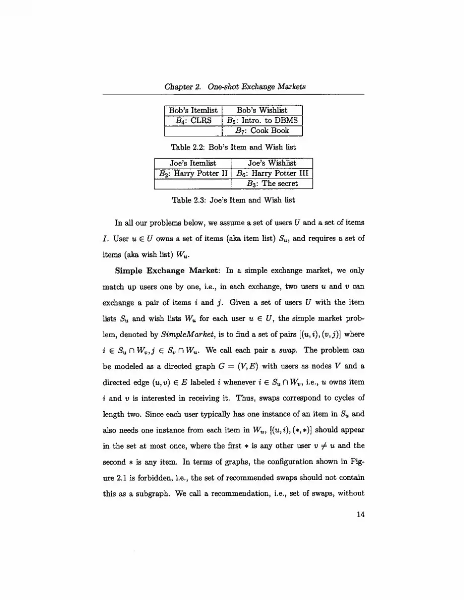
Bob’s Itemlist Bob’s WishlistB4: CLRS B5: Intro, to DBMS
B7: Cook Book
Table 2.2: Bob’s Item and Wish list
Joe’s Itemlist Joe’s WishlistB2: Harry Potter II B6: Harry Potter III
B3: The secret
Table 2.3: Joe’s Item and Wish list
In all our problems below, we assume a set of users U and a set of items
I. User u E U owns a set of items (aka item list) S, and requires a set of
items (aka wish list) W,,.
Simple Exchange Market: In a simple exchange market, we only
match up users one by one, i.e., in each exchange, two users u and v can
exchange a pair of items i and j. Given a set of users U with the item
lists S and wish lists W for each user u E U, the simple market prob
lem, denoted by SimpleMarket, is to find a set of pairs [(u, i), (v,j)] where
i E S fl W,,,j e S fl W,. We call each pair a swap. The problem can
be modeled as a directed graph C = (V, E) with users as nodes V and a
directed edge (u, v) E E labeled i whenever i e S, fl W,, i.e., u owns item
i and v is interested in receiving it. Thus, swaps correspond to cycles of
length two. Since each user typically has one instance of an item in S, and
also needs one instance from each item in W, [(u, i), (*, *)1 should appear
in the set at most once, where the first * is any other user v u and the
second * is any item. In terms of graphs, the configuration shown in Fig
ure 2.1 is forbidden, i.e., the set of recommended swaps should not contain
this as a subgraph. We call a recommendation, i.e., set of swaps, without
14

Chapter 2. One-shot Exchange Markets
Amy’s Itemlist Amy’s WishlistB3: The Secret B2: Harry Potter II
[B8: TAOCP I B4: CLRS
Table 2.4: Amy’s Item and Wish list
Mary’s Itemlist Mary’s WishlistB9: PCs for Dummies B2: TAOCP I
B10: TAOCP II
Table 2.5: Mary’s Item and Wish list
such a forbidden configuration conflict-free. To see why conflict-freedom is
necessary, consider recommending both pairs [(u, i), (v, j)] and [(u, i), (w, j)j
to the users. If user u exchanges i for j with user v, then the recommended
exchange is no longer feasible for user w. Thus, set of recommended ex
changes contains a conflict. The condition above ensures it is conflict-free.
Conflict-free recommendations ensure that users do not get turned off or
lose their trust in their system by finding out that a recommendation they
received from the system is no longer feasible. In our running example (Ex
ample 2.2.1), Joe can give away B2 to both Amy and Alice, but both edges
cannot be in the graph at the same time.
Exchange Markets through Short Cycles. In an online exchange
market, we can find cycles of size larger than 2, for example, as can be seen
in Figure 2.2, we may find users Alice, Bob and Amy with items B7, B4, and
B8. If Alice, Bob and Amy have items B8, B7, and B4 respectively in their
wish lists, we can set up a 3-way exchange among them and have all of them
satisfy their wish lists. Note that, in this example, if we restrict ourselves to
swaps, none of the users may be satisfied. An exchange cycle is a sequence
15

Chapter 2. One-shot Exchange Markets
Figure 2.1: Both exchanges cannot be present in the system at the sametime.
[(ui,ii), (U2,i2),.. . (uk,ik)1, with i,j E fl where j e 1 = j + 1,
1 <j <k, and k e 1 = 1. A set of exchange cycles is said to be conflict-free
provided the pattern [(u, i), (*, *)J appears at most once in the set, i.e., the
corresponding graph does not contain the forbidden subgraph in Figure 2.1.
Our goal is to find an optimal set of conflict-free cycles: The objective
is to maximize the number of items involved in exchanges, thus maximizing
the number of transactions. Furthermore, in practice, we may wish to limit
the length of the exchange cycles to a maximum of k, where k is some
predetermined constant. We usually consider k = 2, ..., 5. The reason why
we focus on short cycles is that, even if one user in the cycle withdraws the
transaction, the whole exchange cycle collapses. If we have long cycles, then
more users would be affected.
16
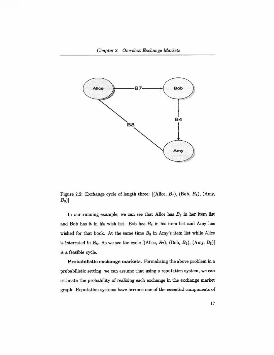
Chapter 2. One-shot Exchange Markets
Figure 2.2: Exchange cycle of length three: [(Alice, B7), (Bob, B4), (Amy,B8)]
In our running example, we can see that Alice has B7 in her item list
and Bob has it in his wish list. Bob has B4 in his item list and Amy has
wished for that book. At the same time B8 in Amy’s item list while Alice
is interested in B8. As we see the cycle [(Alice, B7), (Bob, B4), (Amy, B8)]
is a feasible cycle.
Probabilistic exchange markets. Formalizing the above problem in a
probabilistic setting, we can assume that using a reputation system, we can
estimate the probability of realizing each exchange in the exchange market
graph. Reputation systems have become one of the essential components of
B8
17

Chapter 2. One-shot Exchange Markets
web-based multi-agent systems. These systems gate agents reviews of one
another, as well as about external events, into valuable information [32].
As a result, we have a graph with some probability on each edge. Assuming
that the probability of realizing each edge is independent of other edges, our
goal is to find a set of cycles with the maximum expected number of edges
covered, since each edge corresponds to an item being exchanged. Note
that the probability of a cycle is the product of the probability of its edges.
It would be interesting to understand the complexity of this problem. The
probability P (v) denotes the probability that u is willing to do an exchange
with user v, and pU(j,j) is the probability that user u will exchange item i
with item j, i.e., she gives i and takes j. In this case, the probability of a
cycle being realized will be
P1(u2)x pul(jl,jk) X P2(u3)X FU2(j2,j1). .. x
Puk(ul) x puk(jk,jk_1).
Our goal is to find cycles that maximize the total expected number of items
exchanged.
Example 2.2.2 [Probabilistic Exchange Market]
Consider Figure 2.2 as an example. Let the probabilities associated with
the edges (Alice, Bob), (Bob, Amy) and (Amy, Alice) be 0.7, 0.55 and 0.9.
For simplicity, suppose the probability of this cycle being realized will be
0.7x0.55x0.9 = 0.3465. Let R be a recommendation including this exchange
cycle among others. Then the probability of this cycle being realized will be
0.7 x 0.55 x 0.9 = 0.3465. Let R be a recommendation including this exchange
cycle among others. Then the contribution of this cycle to the value of R,
18

Chapter 2. One-shot Exchange Markets
i.e., to the expected number of exchanged items is 3 x 0.3465 = 1.0395. I
In almost all of the cases, the probability of each edge being realized is
less than one, so when the cycle gets larger, the probability would be very
low. Therefore (similar to what we argued before for the deterministic case)
in the probabilistic case short cycles are practically more appealing.
2.3 Hardness Results
In this section, we show that the SimpleMarket problem is NP-complete.
We also show that the ProbMarket problem is NP-complete, regardless of
whether we consider swaps or short cycles with length bounded by a constant
k > 2. Even the “kidney exchange version” of ProbMarket where every user
owns only one item and wishes for only one item remains NP-complete when
cycles of length> 2 are allowed. We first define the decision versions of these
problems formally.
SimpleMarket Decision Problem
Instance: A set of users U with the item lists
S, and wish lists W for each user u E U.
Question: Does a conflict-free swap cover
C with number of items exchanged K?
The simple market decision version, Probusr associates with every user
a probability that she will transact with any user. Probjtm associates with
each user and a pair of items i,j, a probability that the user will give i and
take j in exchange.
19

Chapter 2. One-shot Exchange Markets
ProbMarket Problem
Instance: A set of users U with the item
lists S and wish lists W for each user u e
U and two probability assignment functions
Probusr : U x U —* [0, lj and Probjtm : U x
IxI—[O,1].
Question: Does a cycle cover C whose ex
pected number of items is > K?
We next define TriEdgePart, a well-known NP-complete problem. We
will reduce this problem to our problem.
TriEdgePart Problem
Instance: A tripartite graph G with three
vertex partitions (X, Y, Z) and an edge set
EcXxYUXxZUYxZ
Question: Does an edge partitioning of G
into disjoint sets of cycles of size three?
Finally, we define 4CycEdgePart, a problem involving 4-partite graphs.
We will find it convenient to use this problem as an intermediary in our
reductions.
20

Chapter 2. One-shot Exchange Markets
4CycEdgePart Problem
Instance: A 4-partite graph G with four ver
tex partitions (X, Y, I, J) and a collection of
edges E consisting of a subset of edges from
Xx YUX x IUY x J, together with a multiset
of edges from I x J.
Question: Does an edge partitioning of G
into disjoint sets of cycles of size four?
We first show that the 4CycEdgePart problem is NP-complete and
then give a reduction from 4CycEdgePart to SimpleMarket showing NP-
completeness of SimpleMarket.
Theorem 1 The 4CycEdgePart problem is NP-complete.
Proof: The membership in NP is straightforward: given an edge par
titioning P of C, we can check in polynomial time whether P consists of
4-cycles that are pairwise edge-disjoint, covering all edges of C. To prove
the hardness, we give a reduction from TriEdgePart. The triangle edge-
partitioning of tripartite graphs is known to be NP-complete (and in fact
APX-hard) by a result of Abraham et. al [6], following an NP-completeness
by Holyer [20].
Given an instance G(X U Y U Z, E) of TriEdgePart, we construct an
instance G’ (X’ U Y’ UI’ U J’, E’) of 4CycEdgePart as follows: for any vertex
w E Z, we add two corresponding vertices w e I’ and w2 e J’; for each
u X, we add a vertex u’ E X’; and for any v E Y, we add a vertex v’ e Y’.
21

Chapter 2. One-shot Exchange Markets
In other words, we let
= ixi, I1’I = 11,1 = I.”! =
i.e., we choose X’, Y’ to be any sets with size lxi, iYl and I’ and J’ to
be any sets with size IZI, with X’, Y’, I’, J’ being pairwise disjoint. Then,
we construct edges E’ (G’) of the new instance as follows: for any edge
(u,v) e E(G) where u e X and v e Y, we add an edge (u’,v’) to E’(G’); for
any edge (u, w) E E(G) where u E X and w E Z, we add an edge (u’, w1)
to E’(G’); and for any edge (v, w) E(G) where v e Y and w e Z, we
add an edge (v’, w2) to E’(G’). Finally, we add de(w) edges between every
pair w1 E I’ and w2 E J’ (corresponding to a vertex w € Z). Note that
deg(w) is even in our case, otherwise it is clear that there is no triangle
partitioning. The reason that we put des(w) edges is that there may be more
than one triangle passing through w E Z, and each triangle corresponds
to two edges for passing through any node, therefore to maintain the same
number of cycles in the 4-partite graph, we need to connect w and w2
with dew) edges. Clearly, G(X’ U Y’ U I’ U J’, E’) is an instance of the
4CycEdgePart problem. It should also be noted that while instances of
the TriEdgePart are always simple graphs, instances of the 4CycEdgePart
can be multi-graphs since we need multiple edges between w1 and w2, for
various w E Z. However,they are not arbitrary multi-graphs: e.g., between
x E X and y e Y at most one edge is required (see the formal definition of
the 4CycEdgePart decision problem above).
22

Chapter 2. One-shot Exchange Markets
Now, we formally show that there exists an edge-partitioning of edges of
G into edge-disjoint triangles if and only if there exists an edge-partitioning
of G’ into edge-disjoint 4-cycles. Consider an edge-partitioning T of edges
of C to edge-disjoint triangles T = {((xiylzl),... , (x,yz))} for p = E(G)I
For each triangle XjjZj in this edge-partitioning T where x E, y2 E Y, and
z. e Z, we associate a corresponding 4-cycle x’y’z1z2 in C’ where x’ e X’,
y’ E Y’, and zi E I’, and z2 E J’. Since the edges of p triangle (xjyjzj) for
1 i p cover all edges of G, each vertex z e Z appears exactly in
triangles. Let T’ be the set of corresponding 4-cycles to triangles in T. Thus,
there are exactly 4-cycles in T’ corresponding to triangles in T, and as
a result, T’ is also an edge-partitioning of G’ into edge-disjoint 4-cycles. Now,
consider an edge-partitioning T’ of G’ into edge-disjoint triangles. Similar
to the above construction, we can construct a set T of triangles partitioning
the edges of G to p edge-disjoint triangles. The above two facts show that
there exists an edge-partitioning of edges of C to edge-disjoint triangles if
and only if there exists an edge-partitioning of C’ to edge-disjoint 4-cycles.
This completes the proof of hardness. I
We next show:
Theorem 2 The SimpleMarket problem is NP-complete.
Proof: Once again, membership in NP is straightforward: given a set
swaps, it is easy to check whether it is conflict-free and the number of
items covered is K. To prove the hardness, we give a reduction from
4CycEdgePart to the SimpleMarket problem.
23

Chapter 2. One-shot Exchange Markets
Figure 2.3: Hardness Proof
24

Chapter 2. One-shot Exchange Markets
Given an instance G(X U Y U I U J, E) of the 4CycEdgePart problem,
we construct an instance E of the simple marketing problem as follows: we
let the set of users be X U J, and the set of items be I U Y. For each user
XE X, we set the item list of x to S = {i Eli (x,i) E E(G)} and the wish
list of x to W = {y E J (x,y) E E(G)}. Similarly, for each userj E J, we
set the item list of j to S, = {y E Y (y,j) E E(G)} and the wish list of j
to Wj = {i E I (i,j) E E(G)}.
Now, we show that there exists an edge-partitioning of G into p =
edge-disjoint 4-cycles if and only if there exists a conflict-free set of p swaps
between pairs of users in the instance of the simple market exchange
problem. Consider an edge-partitioning T of G into p edge-disjoint 4-cycles
T = {(x,y,j,i)i1 v p}. In any 4-cycle (Xv,yv,iv,jv) clearly x E X,
Yv E Y, iv E I, and Jv E J. Consider the corresponding possible swap where
x gives item iv to user v and receives item Yv in return from v. By the
construction of item and wish lists, this swap is feasible. Let S be the set of
swaps derived from T. Clearly Si = p. We show S is conflict-free. Suppose
not. Then there is a pair of swaps in $ of the form: user a swaps item a for
item /3 with user b and a also trades a for item y with user c (which may or
may not be b). This implies T contains two 4-cycles which share the edge
(a, a), a contradiction to the edge-disjointness of T.
Now, suppose S is any conflict-free set of p swaps for the instance D.
We construct an edge-disjoint 4-cycle cover T as follows. For every swap
where user a trades a for /3 with user b, choose the corresponding 4-cycle
(a,a,b,/3,a). It is easy to show T covers all edges of G and it is pairwise
edge-disjoint. This completes the reduction and the proof. •
25

Chapter 2. One-shot Exchange Markets
We next turn our attention to the ProbMarket problem. The follow
ing restricted versions are particularly interesting. First, what can we say
about ProbMarket when we restrict attention to swaps, i.e., when we are
interested in finding an optimal conflict-free set of swaps? The hardness
for the corresponding deterministic case implies the probabilistic version is
hard as well. In particular, the deterministic version is a special case when
all probabilities are set to 1. Second, suppose every user owns just one item
and wishes for just one item. This is similar to the kidney exchange problem
and we call it the “kidney exchange version” of ProbMarket. If exchange
cycles with length more than two are allowed, by the result of [5], it follows
that this problem is NP-complete. When only swaps are allowed, the same
technique of finding maximum weighted perfect matching can be used to
solve this problem exactly in polynomial time. We thus have:
Corollary 1 Finding an optimal set of swaps for ProbMarket is in general
NP-complete. However, for the kidney exchange version, the problem can be
solved in polynomial time. Finding an optimal conflict-free set of exchange
cycles where cycle length is bounded by k > 2 for the kidney exchange version
of ProbMarket is NP-complete.
2.4 The Algorithms
In this section, we develop four algorithms for variants of the exchange
market problem. Three of them have provable approximation bounds w.r.t.
optimal algorithm. The remaining one is a heuristic algorithm with no such
guarantees. However, as we will see shortly, it is much more efficient than the
26

Chapter 2. One-shot Exchange Markets
approximation algorithms. While theoretically the heuristic algorithm may
not sound interesting compared to the approximation ones, we study their
relative performance on synthetically generated data sets in Section 2.6.
Some of these algorithms are inspired by algorithms for the set packing
problem. In section 2.5, we define the weighted k-set packing problem and
show that the exchange market problem can be seen as a special case of the
set packing problem. We exploit this connection to derive the approximation
bounds.
In the rest of the paper, we will find it convenient to deal with a graph
representation of market exchange problems. Given a (simple or short-
cycles) market exchange problem instance E = (U, I, {S I u e U}, {W Iu e U}), with users U, items I, item lists S and wish lists W, the cor
responding graph representation GE is defined as follows. GE is a directed
edge-labeled graph and has a node for every user in U. There is a directed
edge (u, v) labeled i whenever i E I is an item such that i E S fl Wi,. For
our running example of Example 2.2.1, the corresponding graph is shown in
Figure 2.4.
2.4.1 Algorithm Maximal
One heuristic algorithm is to look for a maximal set of cycles in GE. S is a
maximal set of cycles if S is conflict-free and there exists no cycle C in GE
which does not appear in S and does not conflict with any cycle in S.
Example 2.4.1 [Maximal vs. Optimal]
Let’s consider the following cycles in the running example:
27

Chapter 2. One-shot Exchange Markets
Figure 2.4: Graph Representation of Running Example.
28

Chapter 2. One-shot Exchange Markets
C1 = [(Alice, B7), (Bob, B4), (Amy, B8)], C2 = [(Alice, B7), (Bob, B4),
(Amy, B10), (Mary, B9)], and C3 = [(Amy, B3), (Joe, B2)]
Two sets S and S2 are maximal:
S1 = {c1,c3} and 52 = {c2,CS}. Note: coverage(Si) ={B7,B4,B8,B2,B3}
and coverage(S2)= {B7,B4,B10,B9,B2,B3}. Both are maximal since no
cycles can be added to either without breaking the conflict-freedom property.
Furthermore, notice that coverage(S1) coverage(S) and coverage(S2)
coverage(S1). However, Si is clearly not optimal since S2 covers strictly
more items. I
In order to find the maximal set of cycles, we first initialize the set of
cycles B to 0. Then for a random node v E V(G) we perform a breadth first
search (BFS) or a depth first search (DFS) from v to find a cycle. While
performing the BFS/DFS the first time that we encounter a backward edge
we can stop because a cycle has been found. BFS will find the shortest cycle.
And terminate if no cycles are found. Add C to B, and remove all edges
that are in conflict with C from the graph. Set C to 0 again and start the
BFS from another node. We repeat this procedure M times and select the
result with maximum weight. In Section 2.6, we explore the performance
of this algorithm for different choices of M. The complete description of
Algorithm Maximal is depicted in Figure 2.4.1.
2.4.2 Greedy Algorithm
Another approach is to perform a greedy algorithm. Initialize B to 0. At
each step find the best exchange cycle C with the maximum weight. In
29

Chapter 2. One-shot Exchange Markets
order to find the best cycle, we should try all short cycles and then pick the
cycle with maximum weight. Then add C to the set of cycles 13. Remove
all the edges that are in conflict with C. Add C to 13 and if no cycles are
found terminate. The complete description of Algorithm Greedy is depicted
in Figure 2.4.2.
2.4.3 Local Search Algorithm
In this algorithm we attempt to replace a small subset of the current solution
by some set of cycles that result in a greater total weight. Let the current
solution be 13. For any exchange cycle C that is not afready selected, try to
add C and remove all the conflicting edges. If the total weight of B increases
by a factor /3, add C to B and update 13 by removing all conflicting cycles
from 13. Do this procedure until no local improvement is possible, output
B and terminate. The complete description of Algorithm Local Search is
depicted in Figure 2.4.3.
2.4.4 Greedy/Local Search
Instead of starting the Local Search algorithm with an empty set, we can
seed it with a good set of cycles. A variant is to run the greedy algorithm to
find a set of cycles B and then run the local search algorithm starting from
cycles in 1.3. Analysis of this variant is presented in Section 2.5.
30

Chapter 2. One-shot Exchange Markets
2.5 Analysis
2.5.1 Performance
In order to prove approximation factors for the algorithms proposed in this
paper we link our problems to the weighted k-set packing problem. We show
that the simple market exchange problem can be formalized as a special
case of the weighted k-set packing problem. Note that the purpose of this
formulation is solely for the purpose of deriving approximation bounds.
In the weighted k-set packing problem, given a collection of sets, each of
which has an associated weight and contains at most k elements drawn from
a finite base set, our goal is to find a collection of disjoint sets of maximum
total weight. The restriction to sets of size at most k properly includes
multi-dimensional matching, which is a generalization of the ordinary graph
matching problem. Weighted k-set packing is proved to be NP-hard for any
k 3, even in the unweighted case [15], and heuristics and approximation
algorithms have been developed for this problem.
To formulate the one-shot exchange market problem as a special case
of the set packing problem, we define the elements of the sets to consist of
the user, the item, and the act of giving or wishing. The formulation is as
follows:
First, enumerate all exchange cycles of length k. This can be done
in polynomial time since k is a constant. Construct a set corresponding to
every exchange cycle. To illustrate, consider an exchange cycle where user
u gives item i to user v and wishes item j in return. The elements of the
set are:
31

Chapter 2. One-shot Exchange Mai*ets
(u gives i) denoted by
(v gives j) be denoted by x.
(u wishes j) be denoted by
(v wishes i) be denoted by y,,.
Thus, the set corresponding to the above exchange is
{xu,j,xv,j,yu,j,yv,j}
In the above notation, x is a symbol for “giving an item” and y for
“wishing an item”. The first term in the subscript shows the user involved
in gives/wishes relation and the second term is the item being exchanged.
Set the weight of each set constructed to be the cardinality of the set. For
a probabilistic variant, set the weight to be the cardinality times the product
of probabilities associated with the exchartge cycle. Let w(C) denote the
weight of a cycle (equivalently, set) C.
In each of the exchange problems, our objective is to find a conflict-free
set of exchange cycles B such that cEBw(C) is maximized. This exactly
corresponds to weighted k-set packing.
We proved in Section 2.3 that the simplest case of our problem which
is the simple marketing problem is NP-complete. We also showed that
the probabilistic exchange market problem is NP-complete. Here, using
the above reduction to the k-set packing problem, we obtain approxima
tion bounds on Algorithms Greedy, Local Search and Greedy/Local Search.
The approximation bounds proved in the literature for these algorithms for
32

Chapter 2. One-shot Exchange Markets
weighted k-set packing carry over to our exchange problems since the latter
can be seen as a special case of weighted k-set packing.
• Algorithm Maximal: It is not obvious how close the solution of this
algorithm will be to the optimal solution. The reason is that the BFS
algorithm is performed from an arbitrary node and picks the first cycle
that is found.
• Algorithm Greedy: In [10], the authors show that performance of a
greedy approach to the weighted k-set packing problem gives us a 2k-
approximation. That is, in the worst case total weight of the output
would be of the total weight of the set of maximum weights. The
factor 2k is because from the sets that are removed in each iteration,
the optimal solution can contain at most 2k sets, at most one for each
element of the selected set all of which are of weight at most that of
our selected set. They also state that this factor cannot be improved.
• Algorithm Local Search: Using a result in [8] we can show that this
algorithm is a 2k — 1-approximation, meaning that in the worst case
the total weight of the given solution would be 1/(2k — 1) of the total
weight of the optimal solution.
• Local Search/Greedy Algorithm: In [10] the local search/greedy al
gorithm is proved to have a performance ratio of 2(2k + 1)/3 and that
this ratio is asymptotically tight.
33

Chapter 2. One-shot Exchange Markets
2.5.2 Running Time
In the following, the number of cycles that are found is depicted by 131. The
worst case running time of the proposed algorithms are as follows:
• Maximal Algorithm: The running time of this algorithm is 0 ((I V I +
El)113l). Each BFS will take O(IVI + IEI) time. In the worst case the
number of cycles that are found is 13!.
• Greedy Algorithm: Finding the best cycle in each step takes 0(1 V 2k)
time, thus the total running time will be 0(IVl2dlBl)
• Local Search: In the local search algorithm, the running time of check
ing all cycles is 0(lVl2c). In order to check if each cycle is in conflict
with the cycles in the current solution at most 0(IEI) time is needed.
At each step, we perform the local operation if it increases the weight
of the solution by more than a 1+ e factor, where e is a small constant.
Therefore, the number of local operations will be log1OPT where
OPT is the weight of the optimum solution. Thus the worst case run
ning time for the local search algorithm will be: Q(V2kElog OPT).
• Greedy/Local Search: The running time of this algorithm simply is the
addition of the greedy and local search algorithm, because the results
of the greedy algorithm will be input to the local search algorithm.
2.6 Experimental Results
We implemented the Maximal, Greedy, and Local Search algorithms using
MATLAB. The experiments were run on a Computer with a 2.160Hz Intel
34

Chapter 2. One-shot Exchange Markets
Core 2 Duo CPU and 1 GB of RAM under Windows XP.
The goals of our experiments are as follows:
• Obviously, allowing exchange cycles of length more than two will make
for increased coverage of users/items. We wish to study the impact
of allowing cycles of length more than two on the extent to which
coverage increases.
• To examine the quality of the results found by algorithms, especially
the Maximal algorithm which does not have a guaranteed approxima
tion factor.
• To study the scalability of Algorithm Maximal and also the impact
of the parameter M (number of repeated trials) on the quality of the
output.
2.6.1 Data Set
We could not get access to the data of real online exchange applications.
Hence, we generated a set of synthetic data. The intuition behind the data
generation is that the popularity of items in wish lists and item lists follow
some power law distributions, i.e., there are many items which are wished
for or provided by a small number of people, and there is a small number
of items which are provided or wished for by many people. To achieve this
goal, first, we generate some power law distributions with a given power as
the parameter. We actually examined four different powers of 0.5, 1, 1.5
and 2. We use one of these power law distributions for the popularity of
the items, i.e., the number of people who own one item. We also generate a
35

Chapter 2. One-shot Exchange Markets
set of item list sizes based on some other power law vectors (this is justified
by the fact that the size of wish lists and item lists should also follow some
power law distribution). We also generate a vector of wish list size in direct
correlation with the vector of item list sizes. The intuition here is that if
a user provides more items, then probably she has larger wish lists as well.
This intuition is not true in all cases, so we add some noise to this process
with a small probability.
Now, given a popularity vector, and the two vectors of the wish list and
item list sizes, we generate the real wish lists and item lists as follows. For
each item to be added to an item list or wish list, we generate an item
independently from the popularity vector. This process ensures that the
expected number of appearances of items in item lists and wish lists follow
some power law distribution.
2.6.2 Experiments
In order to achieve our experimental goals above, we performed the follow
ing experiment. First we just considered cycles of length two (1 = 2) and
observed the number of items involved in cycles. In the next steps we allow
cycles of length three (1 = 3), four (1 = 4) and then five (1 = 5) and measured
the increase in the number of items covered compared to the previous cases.
We didn’t go beyond 1 = 5 since as mentioned in Section 3.3 long cycles
are not of interest in the market exchange problems studied in this paper.
We ran our algorithms on three different data sets with 10, 000, 25,000 and
50,000 users.
Table 2.6 summarizes the results of the algorithms in form of average
36

Chapter 2. One-shot Exchange Markets
amount of increase in coverage as the allowed cycle length is increased from
2 to 5. It is interesting to note that the extent of incremental coverage drops
as the allowed cycle length 1 is increased from 2 to 5. This is consistent for all
three algorithms. This can be explained by the small world phenomenon of
networks following power law distributions. Beyond a certain length, cycles
of longer length tend to pay “diminishing returns” in terms of %increase
in the coverage. The figures in the table correspond to the data set of
size 10, 000, averaged over various a = 0.5, 1.0, 1.5, 2.0. We observed little
variance over different values of a.
%Increase 2—3 3—”4 4—*51Maximal Aig. 5.56 3.40 2.7Greedy Mg. 7.33 3.81 3.12
Local Search Alg. 7.71 3.85 3.35
Table 2.6: % Increase in coverage when considering cycles of length 3, 4 and5.
Figures 2.8, 2.9 and 2.10 illustrate results of the experiments for
maximal, greedy and local search algorithms respectively. In all figures,
“size of data set” refers to the number of users.
First, for any of the algorithms, the number of items covered for any fixed
value of 1 decreases as the skew factor a increases. E.g., in Figure 2.8, at
a = 0.5 and I = 4, about 50,000 items are covered by the recommendations
generated by Algorithm Maximal on the data set of size 25,000. On the
same data set and 1, at a = 2.0, this number drops to about 15,000. The
same trend can be observed in the plots for other algorithms. The reason
this happens is as the data is more skewed, fewer users own or wish for any
reasonable number of items. Thus, the number of users who can engage in
37
Chapter 2. One-shot Exchange Markets
fruitful exchanges decreases which in turn brings down the number of items
covered.
Second, while theoretically, Algorithm Maximal does not enjoy any prov
able approximation guarantees, the quality of its output is comparable to
that of the other algorithms. E.g., consider Figures 2.8, 2.9, and 2.10 and
examine the number of items covered by the algorithms for the following
situation: 1 = 4 and a = 1,1.5, and data set size = 25,000. For a = 1.0,
the maximal algorithm achieves a coverage of about 60, 000 items whereas
both greedy and local search achieve about 65,000. Similarly, for a = 1.5,
maximal achieves about 35,000 compared to about 41, 000 achieved by both
greedy and local search.
Next, Figure 2.12 compares the average of the running times of the
algorithms. The figure shows the running times averaged over various values
of a. As expected, the running time of the Maximal algorithm is much better
than that of the two other algorithms. Taken together with the fact that
the quality of the output of Algorithm Maximal is found to be comparable
to that of the other algorithms, this makes it a serious contender for finding
a conflict-free set of exchange cycles with good coverage.
To compare running time of the algorithms according to different values
of a, we plot the running times of the algorithms on datasets of size 10000,
25,000 and 50,000 over various values of a = 0.5,1, 1.5, and 2. As we can see
in all Figures 2.13, 2.14, 2.15, 2.16, 2.17, 2.18, 2.19, 2.20, and 2.21 running
time of the algorithms decreases as the value of a increases.
Another parameter that was explored was the number of times the
maximal algorithm (denoted as M in the Section 2.4) is run in order to
38

Chapter 2. One-shot Exchange Markets
get a reasonable result quality in a reasonable time. We examined M =
20, 50, 100, 120. The results are illustrated in Figure 2.11. The result qual
ity, measured in number of items covered, improves significantly when M
is increased from 20 to 50. From 50 to 100, the increase drops and finally
from 100 to 120, the increase is almost negligible. We selected M = 100 in
all our experiments.
2.7 Conclusion
In this chapter, we study various models for the one-shot exchange market
problem, prove that all of these problems are NP-hard and propose several
heuristic and approximation algorithms for these problems. We analyzed
the approximation algorithms by showing some worst-case approxima
tion guarantees.
In the deterministic case, we motivated simple market exchange where
only exchanges in the form of swaps are acceptable. While for a very similar
kidney exchange problem, this is solvable in polynomial time, we proved that
this is NP-complete in our case. When longer exchange cycles are allowed,
NP-completeness extends to our setting. We also proposed a probabilistic
exchange market problem where there are probabilities associated with a
user engaging with another in an exchange and with exchanging one item
for another. The hardness results extend to this case.
By leveraging a close connection to weighted k-set packing, we developed
a heuristic algorithm (Maximal) and approximation algorithms (Greedy, Lo
cal Search, and Greedy/Local Search). Using this connection, we showed
39

Chapter 2. One-shot Exchange Markets
that known approximation bounds for these algorithms for wighted k-set
packing carry over to our exchange market problems — both deterministic
and probabilistic.
Finally, we conducted a detailed experimentation using synthetically
generated data sets, comparing different algorithms on output quality and
running time and studying the extent of increase in coverage as maximum
cycle length is increased, as well as the impact of data skew on coverage.
Our results show that while Maximal does not have provable approximation
guarantees, its performance in practice may be comparable to that of the
other algorithms. This is interesting given that Maximal is by far the most
efficient.
40

Chapter 2. One-shot Exchange Markets
Algorithm Maximal:
1. Repeat M times:
(a) Construct a graph G from theexchange market instance.
(b) Initialize the set of cycles 13 to bethe empty set.
(c) While there exists a cycle in graphG:
i. Run a BFS algorithm on graphC starting from a randomnode to find a cycle C in thegraph.
ii. Add cycle C to the set of cyclesB.
iii. Remove edges of C and allother conflicting edges of Cfrom graph G.
2. Select the maximum weight set amongthe M sets that are found.
Figure 2.5: Description of the Maximal Algorithm
41

Chapter 2. One-shot Exchange Markets
Algorithm Greedy:
1. Construct a graph G from the exchangemarket instance.
2. Initialize the set of cycles 13 to be theempty set.
3. While there exists a cycle in graph G:
(a) Find an exchange cycle C of size atmost 2k with the maximum weightin graph C.
(b) Add cycle C to the set of cycles 1.3.
(c) Remove edges of C and all otherconflicting edges of C from graphC.
Figure 2.6: Description of the Greedy Algorithm
42

Chapter 2. One-shot Exchange Markets
Algorithm Local Search:
1. Construct a graph G from the exchangemarket instance.
2. Initialize the set of cycles B to be theempty set.
3. At each step
(a) Let the current set of cycles be B.
(b) For any exchange cycle C that isnot already picked,
i. 1y to add C, and remove allcycles in B in conflict with C.
ii. If the total weight of B increases, add C to B andremove all conflicting cyclesfrom B.
(c) If no local improvement is possible,output B and terminate.
Figure 2.7: Description of the Local Search Algorithm
43

Chapter 2. One-shot Exchange Markets
10 Alpha = 0.5, Maximal Algonthm io Alpha = 1.0, Maximal Algorithm
a,0)
-C
10a,
2I = 33
I I = 414 EI = 5Il=5
___________________
C C10000 25000 50000 10000 25,000 50000
Size of Datasets Size of Datasets
x 1 Alpha = 1.5, Maximal Algorithm x 1 o Alpha = 2.0, Maximal Algorithm
a,a,-C-C
_______
° 1.:
_____
a,
_______
D =4
________
0.5
____
C C10000 25,000 50000 10000 25000 50000
Size of Datasets Size of Datasets
Figure 2.8: Results of the Maximal algorithm on datasets of size 10000,25000 and 50000.
44

Chapter 2. One-shot Exchange Markets
Figure 2.9: Results of the Greedy algorithm on datasets of size 10000, 25000and 50000.
- x io4 Alpha = 0.5, Greedy Algorithm
8
6
4
2
0a)0)
(U
C.,‘Ca,U)Ea,
0
.0a,Ez
•0a,0)C
C.)‘Ca)
0
.0a,Ez
1 Alpha = 1.0, Greedy Algorithm15
0)
10
05
a, Il=4
050000 10000 25,000 50(
Size of Datasets
x io4 Alpha 2.0, Greedy Algorithm3
lö000 25,000Size of Datasets
x io4 Alpha = 1.5, Greedy Algorithm
)00
0a,‘ 2.5(U
C) 2a,
1.5
.0a,
0.5z
10000 25,000Size of Datasets
50000 10000 25,000Size of Datasets
50000
45

Chapter 2. One-shot Exchange Markets
V(U0)C(U
0x(UCi)
E(U
0
.0(UE2
10ilpha = 0.5, Local Search Algorithm ioA1la = 1.0, Local Search Algorithm
(U0)C(U
0x(U(1)E0)
0
.0(UEz
Va)0)CCU
0x(UCaE(U
0
.0(UEz
Va)0)CCU
C.)x(UCl)E(U
0
.0(UE2
25,000 25,000 50000Size of Datasets Size of Datasets
Figure 2.10: Results of the Local Search algorithm on datasets of size 10000,25000 and 50000.
5.5
aCl
3.5
2.5
—4-----
—4—23—,4
----—---
20 50 100 120M
Figure 2.11: Percentage of coverage for different M’s in the Maximal algorithm.
46

Chapter 2. One-shot Exchange Markets
E
2
Figure 2.12: Average Running Time of Various Algorithms.
2018
. 16
E 141210
c 8CC
2420
Maximal, size = 10,000
0.5 1 1.5 2
Alpha
Figure 2.13: Running Time of Algorithm Maximal on dataset of size 10,0000over various aiphas.
Sire
EEEz- -
z ---
--L2
— Lz5
47

140
120
100
80
60
40
20
0
200180
- 160• 140
120100
c 80CC
- 4020
0
Maximal, size 25k
Maximal, size 50k
0.5 1 1.5 2
Alpha
Figure 2.15: Running Time of Algorithm Maximal on dataset of size 50,0000over various alphas.
Chapter 2. One-shot Exchange Markets
C
6V6•1
VICCC
1
0.5 1 1.5 2
—L5
Alpha
Figure 2.14: Running Time of Algorithm Maximal on dataset of size 25,0000over various aiphas.
L3
— L5
48

Chapter 2. One-shot Exchange Markets
120C.100a)E 80
I
Greedy, size = 10k
0,5 1 1.5 2
Alpha
Figure 2.16: Running Time of Algorithm Greedy on dataset of size 10,0000over various aiphas.
1400
1200C
1000
800
p600
400
200
0
Greedy, size 25k
0.5 1 1.5 2
Alpha
—L5
Figure 2.17: Running Time of Algorithm Greedy on dataset of size 25,0000over various aiphas.
140
--L2
L3
---_
--
-
49

2500
2000
E1500
1000CC
500
0
Chapter 2. One-shot Exchange Markets
Greedy, size 50k
0.5 1 1.5 2
Alpha
Figure 2.18: Ri.mning Time of Algorithm Greedy on dataset of size 50,0000over various aiphas.
180
160140
.. 120
100
80Cc 60C
4020
0
local Search, size = 10k
Figure 2.19: Running Time of Algorithm Local Search on dataset of size10,0000 over various alphas.
____
—
—
——L=3
—L5
—--
:
----.-
—k——L4
—L5
0.5 1 1.5 2
Alpha
50

Chapter 2. One-shot Exchange Markets
4000
3500
3000E
2500
2000
,E 1500C
1000
500
0
Local Search, size 25k
1 2 3 4
Alpha
Figure 2.20: Running Time of Algorithm Maximal on dataset of size 25,0000over various alphas.
-__
--
-__
--
— —
Figure 2.21: Running Time of Algorithm Maximal on dataset of size 50,0000over various alphas.
- --L3
—15
Local Search, size 50k500045004000350030002500200015001000
5000
-LM
—L5
0.5 1 1.5 2
Alpha
51

Chapter 3
Online Exchange Markets
Over Time
3.1 Introduction
In Chapter 2, we considered online exchange markets under deterministic
and probabilistic models. The objective in those one-shot models was to
maximize the weight of cycles where weight of a cycle could either be de
fined as the number of items/users involved in an exchange cycle (in the
SimpleMarketProblem and CycleMarketProblem) or the expected number
of items/users involved in the transaction in the ProbMarektProblem.
In this chapter we are considering online exchange markets over time
and designate following objectives as well as the objective to maximize the
expected number of items exchanged.
• Maximizing the number (or the total value) of items exchanged in the
market.
• Minimizing the average waiting time of users in the system.
• Maximizing fairness in the system, where by fairness we mean to give
52

Chapter 3. Online Exchange Markets Over Time
higher priority in receiving items to users who contribute more to the
system by sharing more valuable items.
In this chapter we observe that introducing virtual points and a credit
system can decrease the average waiting time by a large margin and also can
help in maximizing fairness in the system. In order to implement a complete
credit system and virtual points, we need to take into account the following
characteristics:
1. Participation: Motivating users for participation in the system by
giving more active users more items.
2. Providing Popular items: Motivating users to provide more pop
ular items by giving more credit to users who provide more popular
items, where an item is more popular if it appears in more wish lists.
3. Encouraging early participation: Motivating users to participate
in the system as early as possible.
4. Fairness: Assigning items to users in the most possible fair way, i.e,
giving items to people who have already collected more credit.
3.2 Related Work
Related work to this chapter can be classified in the following categories:
3.2.1 Scheduling Problems
The problems in scheduling theory that are related to our problem are:
53

Chapter 3. Online Exchange Markets Over Time
Minimum makespan scheduling: Given processing times for n jobs,
P1, P2,. .. , p, and an integer m, find an assignment of the jobs to m identical
machines so that the completion time (makespan) is minimized.
Minimum makespan scheduling problem is NP-hard as we can reduce
2-PARTITION [15] to minimum makespan scheduling on two machines.
Horowitz and Sahni [211 give an FPTAS for the variant of the problem
when there are a constant number of machines. (An algorithm A is said to
be fully polynomial time approximation scheme (FPTAS) if for each e > 0
the running time of A is bounded by a polynomial in the size of instance I
and 1/c.) The minimum makespan problem is strongly NP-hard for arbi
trary m by a reduction from 3-PARTITION [15]. Thus, there cannot exist
an FPTAS for the minimum makespan problem in general, unless P==NP.
Hochbaum and Shmoys [19] give a PTAS ((1 + e)-approximation algorithm
which runs in polynomial time for any fixed e) for the problem. (An algo
rithm A is said to be polynomial time approximation scheme (PTAS) if for
each e> 0 the running time of A is bounded by a polynomial in the size of
instance I.)
Scheduling on Unrelated Parallel Machines: This problem is a
generalization of the minimum makespan scheduling, where the machines are
not identical and a job has different processing times on different machines.
Lenstra, Shmoys, and Tardos [23] give a 2-approximation for this ver
sion. They also proved that it is not possible to approximate it within a
factor (3/2 — e) for any e> 0, unless P=NP. Other generalizations include,
considering precedence constraints in the scheduling of jobs. Lam and Seth
[27] give a (2— 2/ri)-approximation for the version where each job has a unit
54

Chapter 3. Online Exchange Markets Over Time
processing time.
We use the above problems to prove NP-hardness of the fairness maxi
mization problem 3.6.
3.2.2 Fairness Maximization in P2P Systems
The first Peer-to-Peer (P2P) networks were based on the philanthropic be
havior of the peers. However, newer P2P applications such as BitTorrent
incorporate some kind of incentive mechanism to award sharing peers. One
of the main reasons of the recent success of peer to peer (P2P) file shar
ing systems such as BitTorrent is its built-in tit-for-tat mechanism. For
example, a typical Bit- Torrent client uploads to four of its neighbors from
which it receives the most download. The intuition behind such a design is
that it will encourage upload and lead to a fair and efficient allocation of
bandwidth among the peers. In f40] the authors explore if the bandwidth
allocation converges when all the users adopt the above strategy. Such a
dynamic process is intuitively fair as each node returns more to whoever
sent it more. The authors prove that the bandwidth allocation converges to
a market equilibrium. In other words, simple as this appears to be, it indeed
leads to an efficient allocation of bandwidth in the market equilibrium sense.
The P2P systems mentioned above are different from our system. Users
in those systems don’t have lists,and the systems do not generate recom
mendations. Moreover, points and credit system are not defined explicitly.
55

Chapter 3. Online Exchange Markets Over Time
3.3 Model
Consider a set of users U and a set of items I. User u E U owns a set of
items (a.k.a. item list) S, and requires a set of items (a.k.a. wish list) W.
Each item i E I has a value “popularity” P corresponding to it, which is
the number of times it appears in all users’ wish lists.
In our proposed system, the algorithm is run periodically and the set of
potential feasible exchanges are discovered. Users involved in these potential
exchanges are informed through email and/or their account will be updated.
If they are interested in performing the transaction, they will get in touch
with the other users. Otherwise they will withdraw the transaction and all
other involved users will be informed. In any case when the transaction is
done the exchanged items are removed from the item lists and wish lists,
and the system will be updated.
The system is dynamic meaning that it changes with time. The possible
changes are:
• a new user joins the network.
• a user leaves the network.
• an item is removed from a user’s wishlist or itemlist: either of these
changes may be due to a transaction done or the user’s interests
changed.
• an item is added to a user’s wishlist or itemlist.
These changes imply that the set of feasible exchanges will also change by
56

Chapter 3. Online Exchange Markets Over Time
time. Thus, the system runs the algorithm to find the set of new exchanges
that have become available periodically (as an example: once a week).
3.4 Minimizing Average Waiting Time
In this section, we observe that by introducing “virtual points” in the system,
we can decrease the average waiting time of users by a large margin. To
implement this idea, we give virtual points to a user for giving away their
item, and later give them an item for redeeming their points. As an example
let’s assume that user u has item i in their item list and item j in their wish
list. Also, let’s assume user v has item j in their item list, however v does
not have item i in their wish list. Thus, a swap is not possible. The idea
here is that we recommend item j to u and in return give some points to v.
In this case u does not have to wait until v wishes for i or a feasible swap
comes up. We will elaborate on a credit system that implements exchanging
virtual points in the next section. It can be easily seen that, in the worst
case, using virtual points can decrease the average waiting time of users by
a large margin. In the following, we formally show that introducing points
can decrease the expected waiting time, even assuming that all users arrive
in a random order.
Theorem 3 Consider an exchange market consisting of n users, and n
items. Assume that users put their items at n time steps T = 1, 2,. .. ,n,
and we are allowed to assign cycles of size k. Let A be the average waiting
time of users in a system without points and B be the average waiting time
of users in a system with virtual points. There are instances in which in the
57

Chapter 3. Online Exchange Markets Over Time
worse case, A (k — 1)B. Moreover, assuming that users put their items a
random permutation, there are instance in which in expectation A = kB.
Proof: Assume that we can assign cycles of size at most k, and let p =
Consider n users in the system with their item lists and wish lists as follows:
a cycle of size k among users can be formed by having k users u1,... , uj
such that for 1 j < n, user u3 has item i3 in her item list and item
i1 in her wish list and user u has item i in her item list and i1 in her
wish list. Clearly, this instance has admits p = exchange cycles of size
kof. At the beginning, users have empty item lists and will add items in
a random order to their item lists. At the end of the process, user u3 for
1 < j < n will have item i3 in her item list. Starting from empty item
lists, we assume that items become available. In other words, the wish
lists will be posted at the beginning (time T = 0), and items arrive on times
T = 1, T = 2, T = 3,..., T = n, and they are all required in order to complete
p = cycles of length k.
In the case that we use virtual points in the system, as soon as an item
arrives, it will be given to the user that has that item on her wish list.
Therefore the waiting times would be 1, 2,... ,
2
Bn(n+1)
2 2 2
58

Chapter 3. Online Exchange Markets Over Time
In the worst case, all cycles finish in the last k steps of the process. Thus,
in the worst case,
A=kx i=k(n1)_n1) = n(n+1)k2—n(n-i-k)(k—1)B.
i=n—+1
Now, we show that assuming that the items arrive in a random order,
in expectation, A We compute the expected waiting time of users
both in the case that we use virtual points in the system, and in the case
we do not. The expected value of B is the same as in the previous case, i.e.,
B = n(;+1) Now let’s consider the case that we do use virtual points in the
system. Let C2 be a random variable showing the time that cycle i becomes
completed. We also know that the expected waiting time of all cycles being
completed is the same:
E [C1] = E [C2] = ... = E [Cr].
The waiting time in this case would be:
= k>C2.
By linearity of expectations, the expected waiting time is equal to
kE[C]=kpE[C] =nE[C].
59

Chapter 3. Online Exchange Markets Over Time
Now, we compute each E(C) as follows:
E[C]= k
(k_iaL4 (nj=k k
n1 v’111(k)jkk1
k71 j=k j0
—
- (n—k
Therefore, the total expected waiting time is
A = E[C] = nE(C)= kn(n+1)
As a result, the ratio between the expected waiting time with and without
virtual points is 4 =. i
3.5 A Credit System
In this section, we design a credit system that takes into account the prop
erties that we mentioned earlier. We design a credit system in which each
user i collects credit for providing items, and can redeem credit points to
receive some items. Let C(t) be the credit of user i at time t. Each item j
60

Chapter 3. Online Exchange Markets Over Time
has a credit score P3 which can be a function of the popularity of item j.
Initialization: We can initialize the credit of each new user in the system
to zero or a small positive value.
Updating Rules: Consider a transaction T at time t in which a user i
gives an item j to a user i’, i.e, item j is in item list of i and in wish list
of i’. In the following we describe how to choose transaction T and how
to update the credit of each user after transaction T happens to satisfy the
desired properties discussed in the previous section.
• Participation: To satisfy this property, we make sure that we choose
a user i’ to get the item such that C’ (t) is large (perhaps the largest)
among all users who has item j in their wish list.
In general, after transaction T happens, we update C(t+ 1) = C(t) +
Pj(t) and C1(t + 1) = C(t) — P3(t).
• Providing Popular items: To satisfy this property, we set P3 (t) to
be a function of the number of times that item i appears in the wish
lists.
• Encouraging early participation: To satisfy this property, we up
date the scores of users after each time step as follows: Ck (t + 1) =
Ck(t) * (1 + f) where f is a small interest rate, i.e, = 0.001. This will
encourage users to participate in the system as early as possible.
• Fairness: To satisfy fairness in an online way, we should minimize the
maximum credit of a user at each step. As a result, in order to satisfy
fairness, we wait for a period of time (e.g., a day) for users to post
61

Chapter 3. Online Exchange Markets Over Time
new items in their item list (and wish lists), and then assign the items
to other users in the most fair manner. we will formalize this problem
formally in the next section.
3.6 Maximizing Fairness
In this section, we can formalize the fairness problem for assigning all new
items throughout a fixed time window (e.g., one day) to a set of users.
Consider a time step t at which each user has a current credit C2 Let S be
the new set of items in the item list of users during the last time day. Let
W be the wish list of user i, and P be the current value for item j, i.e, if
we give j E W to user i, C(t + 1) = C — Pj. We want to assign items in
sets S to users such that:
• Each item in each item list S is assigned to at most one user.
• If item j S is given to user i’, then j E Wi’.
• Each user i gets at most one copy of item j E W in his/her wish list.
The goal is to find such assignment that minimizes the maximum credit in
the next step, i.e, minmax C(t + i).
The only issue with the above formulation is that it is possible that a
user k with a large credit provide some new items and not assigning these
items may give a better solution since if user k in this situation provides
2We drop the parameter t as it is clear from the context.3The ultimate goal is to find a fair assignment that minimizes the maximum credit,
and subject to this, we minimize the second maximum, and so on, but for the sake ofsimplicity and as a first attempt, we look at the problem of minimizing the maximumcredit.
62

Chapter 3. Online Exchange Markets Over Time
more items, his score increases even more, and as a result the maximum
score increases. Here there is a trade off between the expected waiting time
of users (or similarly the number of items exchanged in the system) and
the above fairness property. A middle-way solution to take into account the
aforementioned trade off is to say that we want to find an assignment of
items in Sj’s to users such that the assignment is maximal and it minimizes
the maximum credit, i.e, after assigning items from item lists to wish lists,
no other item can be assigned from item lists to wish lists of users.
Theorem 4 The fairness maximization problem is NP-complete.
Proof: We give a reduction from a scheduling problem with restricted
assignment (B I ICmax). In a scheduling problem with restricted assignment
(BIICmax), we have n jobs and m machines, and each job j has a processing
time P3 and can be scheduled on a subset U of machines. Given an assign
ment of jobs to machines, where each job j is assigned to a machine in Uj,
the load of machine i, L is the sum of processing time of jobs assigned to
i. The goal is to assign jobs to machines to minimize the makespan or the
maximum load of each machine, i.e., minassignment max L.
There is a clear reduction from the above problem to the max fairness
problem. Here is the reduction: Given an instance of BIICm, we put a
user for each of the n jobs, and also we put a user for each machine i (in
total, we have m + n users). For user i corresponding to machine i, we
have credit C2(t) = C = 0, with empty wish list (W = 0) and a large
item list S with all jobs that can be scheduled on machine i in it (i.e.,
S = {jli E U3}). For user j corresponding to job j in the instance, we
63

Chapter 3. Online Exchange Markets Over Time
put the initial credit C, = Pj, a wish list Wj = {j } and an empty item
list. It is easy to see that an assignment of jobs to machines in the original
B II Cmax problem correspond to an exchange of items in the new instance.
In particular, the load of machine i is equal to the credit of user i in the
new instance. It is clear to see that the problem of minimizing makespan
in the original instance of B I ICmax is equivalent to the fairness problem in
this new instance, i.e, in order to minimize the maximum load of machines
in BlICmax, we should minimize the maximum credit.i
As also mentioned in Section 3.2 the BIICm problem is NP-hard and
not approximable within any constant factor better than 3/2 [23]. B II0max
and the more general version in which the processing time of each job on
each machine is different (i.e, instead of F,, we have is approximable
within a factor 2.
Thus, the above reduction shows that the fairness problem is NP-hard,
and moreover, since the objective functions of the two problems are the
same, if we can optimize the fairness problem within a factor better than
3/2, then we can optimize the BIICm scheduling problem within a factor
better than 3/2.
In Section 3.8 we prove that our problem is not approximable within any
multiplicative factor.
3.7 A Linear Programming Formulation
In this section, we develop an integer linear programming formulation of the
fairness problem. For a triple (i, j’, j) where j S and j e Wi’, let x’j = 1
64

Chapter 3. Online Exchange Markets Over Time
if we assign item j from i’s item list to user i’, and = 0 otherwise. Also,
we let variable t be a variable that corresponds to the credit of user i after
the assignment of this step, and variable t be the maximum of credits, or
maxiEu t. Finally, for easy of notation, we let U be the set of users and I
be set of items.
mm t
tt% VieU
= Cj + Zi’:jEW, jEW Zi’:jES, x’Pj Vi e U
Ei’:jEW1,Xij’j < 1 Vi E U,j Si
Zi’:jES, 1 Vi E U, j e W
Xii’s + i”:jES,,,i”#i i”i’j + Zih’:jEw,,,i”i’ Xii” 1 Vi, j’ E U,j E Si fl T’V’
xjj’j {0, 1} ViVj SVi’ : j e W’
The first inequality indicates that t is the maximum credit of users. The
second inequality quantifies the credit of user i after the assignment. The
third inequality models the constraint that each item j in the item list of
user i can be assigned to somebody at most once, and the forth inequality
models the fact that each item j in the with list of user i can be received by
user i. Finally, the fifth inequality models the maximality of the solution,
i.e, fact that if user i does not give an item j e W’ to user i’, then either
user i gives j to somebody else, or user i’ gets it from somebody else.
The LP relaxation is as follows:
65
Chapter 3. Online Exchange Markets Over Time
mm t
ttj VieU
t = C + j€S Zi’:jEW, x&,P2 ZjEw i’:jESi Vi U
Zj’:jEW1, < 1 Vi e U,j e Si
Zi’:jES2,xjjj 1 Vi U,j e W,
XVi.J + i”:jESn,i”i2i”i’j + 1 Vi,i’ E U,j E S fl T’V
0 1 ViVj SVi’ j e Wi
This LP is similar to the LP for the scheduling problem but has a minus
sign in the inequality for T. It would be interesting to study this LP and
see if a similar approach works. In particular, it would be nice to study the
basic feasible solutions of this LP.
3.8 A Strong Inapproximability Result
In this section, we show that the fairness maximization problem is not ap
proximable within any factor.
Theorem 5 The problem offairness optimization is not approximable within
any multiplicative factor.
Proof: We show that if we can approximate this problem within any
factor, we can solve an NP-complete problem, i.e., the partitioning prob
lem. In an instance of the partitioning problem, we are given n numbers
66

Chapter 3. Online Exchange Markets Over Time
al,a2,. . . a, with the total sum of B = a,, and our goal is to verify if
there exists a partition of these number into two sets such that each subset
has the total sum of . It is known that the partitioning problem is an NP-
complete problem. We say that an instance of the partitioning problem is a
YES instance, if there exists a subset of number of total sum . Otherwise,
the instance is a NO instance.
We give a reduction from the partitioning problem to the fairness prob
lem. In fact, from any instance of the partitioning problem, we construct
an instance of the fairness problem in which the optimal solution to the
fairness problem is greater than zero if and only if the partitioning problem
is a YES instance. Given an instance of the partitioning problem with n
numbers a1,a2,. . . a, where a = B, we construct an instance of the
fairness problem as follows: We put n items and n + 2 users in the instance
of the fairness problem, n users 1,2,3,... , n corresponding to n numbers in
the partitioning problem, and two extra users n +1 and n + 2(that get items
from the first n users). For each user i where 1 n, we put the initial
credit C = —as, wish list W = 0 and item list S = {i}. For two users n+1
and n + 2, we put C÷1 = C+2 = B/2, empty item lists S,÷1 = S÷2 = 0
andW+1=W+2={ij1in}.
Now the optimal solution for the fairness problem is zero if and only if
the partitioning instance is a YES instance. The reason is that the only way
that the credit of both n + 1 and n +2 goes down to zero if and only if both
of these users get a set of items of total credit .
More formally, if the partitioning problem is a YES instance, and there
exists a set S of number of total sum , then set S of users can give items
67

Chapter 3. Online Exchange Markets Over Time
to user n + 1 and the rest of users can give items to user n + 2, and a result
the credit of each user in the next step is zero. Conversely, if the optimal
resulting credit is zero, it means that both users n + 1 and 11+ 2 got exactly
total credit from users 1,2,... , ri. Thus, the set of users who gave an item
to n + 1 construct a subset of numbers with total sum and therefore, the
partitioning problem is a YES instance.
The above shows that if we can verify if the optimal solution for the
fairness problem is zero or any number above zero, then we can distinguish
between the YES and NO instance of the partitioning problem. Therefore,
if there exists an a-approximation algorithm for the fairness problem, it
will output a x 0 = 0 for an instance of the fairness problem with optimal
solution zero. Hence, no approximation algorithm exists for this problem. I
3.9 Heuristic Algorithms
Here, we propose two heuristic algorithms to solve the fairness problem; one
is a simple fast greedy algorithm, and one is based on randomized rounding
of the linear programming formulation discussed in the previous section.
The basic idea of the rounding algorithm is a standard method for solving
integer linear programs.
3.9.1 Greedy Algorithm
A very simple heuristic algorithm is to assign item transfers among users
one by one, and at each step find the one item transfer that minimizes the
maximum credit after this item transfer. In other words, at each step, we
68

Chapter 3. Online Exchange Markets Over Time
examine all possible item transfers for items j E Si fl for any two users i
and i’, and find the triple i, i’, j such that after item transfer, the maximum
credit the minimum possible. To do so, we sort the users in the decreasing
order of their credit, and try transferring items from users at the beginning
of the list.
3.9.2 An LP-rounding Algorithm
Consider the linear programming relaxation discussed for the fairness prob
lem. In the integer linear program x is 1 if use i give an item j e S fl W,i
to user i’. Consider a solution x to this LP. In the LP relaxation, we can
interpret the variable xj to be the extent at which user i gives item j to
user i’. In other words, we use the value as the probability of trans
ferring item j from i to i’. In order to find a feasible solution, we need to
perform the following rounding algorithm.
1. Initialize = 0.
2. Solve the LP relaxation and find an optimal solution x.
3. For each user i and item j E S such that = 0,
(a) Let Z’3 = >
(b) Let = ZiI:Z,j=OXiiIj
(c) Among all users i’ for which > 0 and ij = 0,
i. Choose one user i” with prob probability
ii. Set jj = 1, and S = S— {j}.
69
Chapter 3. Online Exchange Markets Over Time
4. For each item j and each i’ such that j e Wj,
(a) Let set be the set of users i for which jj,j became one in this
round.
(b) If ILi’ I = 1, then for each i” e = 0, and W = W\{j}
(finalize transfer (i”i’j)),
(c) else
i. Choose one user i” e T’ with probability
ii. For each i i” and i Ti’, set ii’j = 0, and S = Si U {j}.
iii. For i”, let = 0, and W’ = W\{j} (finalize transfer
(i”i’j)).
5. If any new item transfer was assigned in the last round, go back to 3
to start a new round, otherwise output and terminate.
3.10 Experimental Evaluation
We implemented the integer linear program formulation of the fairness max
imization problem, linear program formulation of the problem using GNU
Linear Program Kit (GLPK), and also the two heuristics: LP-rounding and
the greedy heuristic using MATLAB. The experiments were run on a Com
puter with a 2.40GHz Intel Core 2 Duo CPU and 3 GB of RAM under
Windows Vista.
The goals of our experiments are as follows:
• To examine the quality of the results found by the heuristic algorithms
70

Chapter 3. Online Exchange Markets Over Time
since we proved that the fairness maximization problem is not approx
imable.
• To study the scalability of the heuristic algorithms and also the impact
of the parameter a.
The LP relaxation discussed in the previous sections gives a polynomial-
time computable lower bound on the optimal value of the fairness optimiza
tion problem. In fact, we use this lower bound to evaluate the performance
of our heuristic algorithms.
3.10.1 Dataset
We could not get access to the data of real online exchange applications.
Hence, we generated a set of synthetic data. Data generation for the markets
over time is similar to what we did in the previous chapter for one-shot
exchange markets which was explained in Section 2.6.1.
3.10.2 Experiments
The following experiments were performed in order to examine the per
formance of the heuristic algorithms. We implemented the integer linear
programming (ILP) and also the linear programming (LP) formulation of
the problem using GLPK and the LP-rounding and the greedy heuristic us
ing MATLAB. We ran our algorithms on three different data sets with 100,
500 and 1000 users. The data were generated with four different values for
a = 0.25, 0.5, 0.75 and 1.
71

Chapter 3. Online Exchange Markets Over Time
users = 10, items = 50
—4—integer Linear Program
—I—— LProunding
—i--Algorithm Greedy
0.25 0.5 0.75 1
Figure 3.1: Performance of the heuristics compared to the optimal solutiongiven by ILP on dataset of 10 users.
We solved the ILP for two small datasets including 10 users, 50 items
and 20 users, 100 items. The ILP gives us the optimal solution however its
running time is exponential. We compare the results of the LP-rounding
and greedy on same datasets to the optimum. The results are depicted in
Figures 3.1 and 3.2 respectively.
Figures 3.3, 3.4, and 3.5 show the results of the LP, LP-rounding and
the greedy heuristic for datasets of size 100, 500, and 1000 respectively. The
number of total items in each case is 5 times the number of users. The Y
axis indicates the maximum credit, and the X-axis shows a for the different
algorithms. We have used the LP results a lower bound on the optimal
value. As can be seen, the LP-rounding has a better performance than the
other heuristic. Also, we can observe that as a increases (in most cases),
120
100
80
E 60
1 40
20
72

Chapter 3. Online Exchange Markets Over Time
Figure 3.2: Performance of the heuristics compared to the optimal solutiongiven by ILP on dataset of 20 users.
the algorithms’ performance also improves.
The running times of the above algorithms are also depicted in Figures
3.6, 3.7, and 3.8 for datasets of size 100, 500, and 1000 respectively. As
can be seen, the running time of the greedy algorithm is better than the LP
rounding heuristic. Moreover, we can see that by increasing a, the running
time improves.
Another measure that we explored was the number of transactions per
formed at each time step. It is important that the users stay active and
have incentive to share their items, even when they have received an item
from their wish list. Figure 3.9 plots the percentage of active users in at
six consecutive time windows in a simulation done with 100 users.
As can be seen at the beginning we have the maximum activity. The
200
users= 20, items = 100
180
160I40
120
10o
. 80
Linear Program
0
0.25 05 0.75
a
73

Chapter 3. Online Exchange Markets Over Time
Figure 3.3: Performance of different algorithms on dataset of size 100.
reason is that all users start with equal initial credits.
3.11 Conclusion
In this chapter, we consider exchange market problems over time and study
efficient mechanisms that improve the users’ waiting times and also give
incentive to users to be more active by maximizing fairness in the system.
In order to achieve the above objectives, we introduce points and credits to
the system and we show that waiting times would improve by using points.
Moreover, we show that the problem of fairness maximization not only is
NP-complete, but also inapproximable. Therefore, we propose two heuristic
algorithms: linear programming-based and a greedy algorithm. We perform
experiments to examine the performance and scalability of the proposed
2500
Dataset size = 100
2000.9
1500
E 1000
0 500
0
-+-LP
—I—. IP-rounding
—i--Greedy
0.25 0.5 0.75
a
74

Chapter 3. Online Exchange Markets Over Time
-__
-_
Figure 3.4: Performance of different algorithms on dataset of size 500.
algorithms. The experiments show that both heuristics perform much better
than the worst-case performance. Moreover, LP-rounding performs better,
however the greedy heuristic is much faster.
Data set size = 5009000
8000
7000
6000
5000
j 4000
3000o 2000
1000
0
-4--LP
—4— LP-rounthng
—i--Greedy
025 0.5 0.75 1
(L
75

Chapter 3. Online Exchange Markets Over Time
Figure 3.5: Performance of different algorithms on dataset of size 1000.
Figure 3.6: Running times for dataset of size 100.
25000
Dataset size = 1000
15000
20000.9
0
E
0
10000
5000
a
S LP-rounding
—*—Greedy
0.25 0.5 0.75
a
Running time, dataset size = 1003000
2500w
2000E; 1500
__________________________________
—I— LProunding1000
500—k—Greedy
a0.25 0.5 0.75 1
U
76

Chapter 3. Online Exchange Markets Over Time
Figure 3.7: Running times for dataset of size 500.
-
E
Figure 3.8: Running times for dataset of size 1000.
running time, dataset size = 50016000
14000
12000
10000
8000
6000 -4—LP-rounding
4000 —i—Greedy2000
0 —
0.25 0.5 0.75 1
a
Running time, dataset size = 100030000
— 25000U
20000E
15000E‘ 10000
•••I••• LP-rounding
I. 5000—-Greedy
0
0.25 0.5 0.75 1
ci
77

Chapter 3. Online Exchange Markets Over Time
I1hiiFigure 3.9: Number of transacting users in 6 consecutive time windows.
User Activity
lIP-rounding
IGreedy
1 2 3 4 5 6
limesteps
78

Chapter 4
Conclusions and Future
Work
In this thesis, we motivate the use of online exchange markets as an appli
cation over social networks and propose specific market exchange problems
where users own item lists and have a list of wishes and can exchange items
with one another. For these problems, we propose a few optimization prob
lems, study the complexity of these problems, propose various algorithms
with guaranteed approximation factor for some of these problems, and fi
nally perform experimental results to evaluate the performance of several
approximation and heuristic algorithms.
In the one-shot deterministic case, we study simple market exchanges in
which the only acceptable exchanges are in the form of swaps. While for a
similar well-studied problem called the kidney exchange problem, this prob
lem is solvable in polynomial time, we prove that this is NP-complete in our
case. When longer exchange cycles are allowed, kidney exchange was shown
to be NP-complete [5] and this extends to our setting. We also propose a
probabilistic exchange market problem in which there are probabilities as
sociated with a user engaging with another in an exchange. The hardness
79

Chapter 4. Conclusions and Future Work
results extend to this case. By leveraging a close connection to the weighted
k-set packing problem, we develop a heuristic algorithm (Maximal) and ap
proximation algorithms (Greedy, Local Search, and Greedy/Local Search).
Using this connection, we show that known approximation bounds for these
algorithms for weighted k-set packing carry over to our exchange market
problems both deterministic and probabilistic. We conduct a detailed ex
perimentation using synthetically generated data sets, comparing different
algorithms on output quality and running time and studying the extent of
increase in coverage as maximum cycle length is increased, as well as the
impact of data skew on coverage. Our results show that while Maximal does
not have provable approximation guarantee, its performance in practice may
be comparable to that of the other algorithms. This is interesting given that
Maximal is by far the most efficient.
Finally, we consider similar exchange market problems over time and
study efficient mechanisms that improve the users’ waiting times and also
give incentive to users to be more active by maximizing fairness in the sys
tem. In order to achieve the above objectives, we introduce points and
credits to the system and we show that waiting times would improve by
using points. Moreover, we show that the problem of fairness maximization
not only is NP-complete, but also inapproximable. Therefore, we propose
two heuristic algorithms: linear programming-based and a greedy algorithm.
We perform experiments to examine the performance and scalability of the
proposed algorithms. The experiments show that both heuristics perform
much better than the worst-case performance. Moreover, LP-rounding per
forms better, however the greedy heuristic is much faster.
80

Chapter 4. Conclusions and Future Work
As a future work, further investigation of these algorithms on real data
sets would be valuable. Designing improved approximation algorithms or
proving some stronger inapproximability results for the optimization prob
lems discussed in this thesis are desirable. Also, it is interesting to study
special variants of these problems that appear in practice, and design approx
imation algorithms with provably improved approximation factor. Finally
it would be interesting to study incentive issues in these settings, and design
mechanisms that perform well in the presence of strategic users who may not
reveal their true parameters (e.g., their item lists). In such settings, users
may lie about their items lists to get a better assignment. To deal with such
settings, one needs to design (truthful) mechanisms that give incentive to
users to reveal their true parameters. It is also interesting to explore if the
proposed mechanism converges to an equilibrium.
81

Bibliography
[1] “http://blog.compete.com/2007/01/25/top-20-websites-ranked-by-
time-spent/”.
[2] http://www.oddshoe.org.
[3] http://www.peerflix.com.
[4] http://www.readitswapit.co.uk.
[5] David J. Abraham, Avrim Blum, and Thomas Sandholm. Clearing
algorithms for barter exchange markets: Enabling nationwide kidney
exchanges. In ACM Conference on Electronic Commerce, pages 295—
304, June 13-16 2007.
[6] David J. Abraham, Ning Chen, Vijay Kumar, and Vahab Mirrokni.
Assignment problems in rental markets. In WINE 2006, pages 198—
213, 2006.
[7] 0. Adomavicius and A. Tuzhilin. Toward the next generation of rec
ommender systems: A survey of the state-of-the-art and possible ex
tensions. IEEE Transactions on Knowledge and Data Engineering,
17(6):734—749, 2005.
82

Bibliography
[8] Esther M. Arkin and Refael Hassin. On local search for weighted k-set
packing. In ESA 1997, pages 13—22, 1997.
[9] M. Blaser and B. Siebert. Computing cycle covers without short cy
cles. In In Proceedings of the S4st Annual European Symposium of
Algorithms, 2001.
[10] Barun Chandra and Magnus Halldorsson. Greedy local improvement
and weighted set packing approximation. In SODA 1999, pages 169—
176, 1999.
[11J W.W. Cohen, R.E. Schapire, and Y. Singer. Learning to order things.
Journal of Artificial Intelligence Research, 10:243—270, 1999.
[12] J. Edmonds and E. Johnson. Matching euler tours and the chinese
postman problem. Mathematical programming, 5:88—124, 1973.
[13] Ozlem Ergun, Gultekin Kuyzu, and Martin Savelsbergh. Collaborative
logistics: The shipper collaboration problem. Computers and Opera
tions Research Odysseus, 2003.
[14] Y. Freund, R. Iyer, R.E. Schapire, and Y. Singer. An efficient boosting
algorithm for combining preferences. In 15th International Conference
on Machine Learning, 1998.
[15] M. R. Garey and D. S. Johnson. Computers and Intractability. Freeman,
New York, 1979.
83

Bibliography
[16] 0. Goldschmidt, D. Hochbauin, C. Hurkens, and C. Yu. Approximation
algorithms for the k-clique covering problem. SIAM Journal of Discrete
Math., 6(3):492—509, 1996.
[17] M. Guan. Graphic programming using odd and even points. Chinese
Mathematics, 1:273—277, 1962.
[18] D. Hochbaum and E. Olinick. The bounded cycle-cover problem. IN
FORMS Journal on Computing, 13(2):104—109, 2001.
[19] Dorit S. Hochbaum and David B. Shmoys. A polynomial approximation
scheme for scheduling on uniform processors: Using the dual approxi
mation approach. SIAM Journal of Computing, 17(3):539—551, 1988.
[20] Ian Holyer. The np-completeness of some edge-partition problems.
SIAM Journal of Computing,, 10(4):713—717, November 1981.
[21] Ellis Horowitz and Sartaj Sahni. Exact and approximate algorithms for
scheduling nonidentical processors. J. ACM, 23(2):317—327, 1976.
[22] N. Immorlica, V. S. Mirrokni, and M. Mahdian. Cycle cover with
short cycles. In Symposium on Theoretical Aspects of Computer Science
(STAGS), 2005.
[23] D. B. Shmoys J. K. Lenstra and Eva Tardos. Approximation algorithms
for scheduling unrelated parallel machines. Math. Program., 46(3) :259—
271, 1990.
84

Bibliography
[24] K. Gallagher. J. Parsons, P. Ralph. Using viewing time to infer user
preference in recommender systems. In AAAI Workshop in Semantic
Web Personalization, July 2004.
[251 R. Jin, L. Si, and C. Zhai. Preference-based graphic models for collabo
rative filtering. In 19th Conference Uncertainty in Artificial Intelligence
(UAI 2003), August 2003.
[26] R. Jin, L. Si, C. Zhai, and J. Callan. Collaborative filtering with de
coupled models for preferences and ratings. In 12th International Con
ference Information and Knowledge Management (CIKM 2003), Nove
meber 2003.
[27] S. Lam and R. Sethi. Worst case analysis of two scheduling algorithms.
SIAM Journal of Computing, 6(3):518—536, 1977.
[28] B.P.S. Murthi and S. Sarkar. The role of the management sciences in
research on personalization. Management Science, 49(10):1344—1362,
2003.
[29] M. E. J. Newman. The structure and function of complex networks.
SIAM Reviews, 45(2):167—256, 2003.
[30] Christos H. Papadimitriou. On the complexity of edge traversing. Jour
nal of the ACM, 23(3):544—554, 1976.
[31] M.J.D. Powell. Approximation Theory and Methods. Cambridge Uni
versity Press, 1981.
85

Bibliography
[32] et al. R. Andersen. Trust-based recommendation systems: an axiomatic
approach. 17th International World Wide Web Conference (WWW),
2008.
[33] B. Rachavachari and J. Veerasamy. A 3/2-approximation algorithm for
the mixed postman problem. SIAM journal of Discrete Math., 12:425—
433, 1999.
[34] P. Resnick, N. Iakovou, M. Sushak, P. Bergstrom, and J. Riedl. Grou
plens: An open architecture for collaborative filtering of netnews. In
Computer Supported Cooperative Work Conference, 1994.
[35] P. Resnick, N. Iakovou, M. Sushak, P. Bergstrom, and J. Riedl. Grou
plens: An open architecture for collaborative filtering of netnews. In
Computer Supported Cooperative Work Conference, 1994.
[36] E. Rich. User modeling via stereotypes. Cognitive Science, 3(4):329—
354, 1979.
[37] G. Salton. Automatic Text Processing. Addison-Wesley, 1989.
[38] G. Shani, R. Brafman, and D. Heckerman. An mdp-based recommender
system. In 18th Conference Uncertainty in Artificial Intelligence, Au
gust, 2002.
[39] Carsten Thomassen. On the complexity of finding a minimum cycle
cover of a graph. SIAM J. Comput., 26(3):675—677, 1997.
[40] F. Wu and L. Zhang. Proportional response dynamics leads to market
equilibrium. In STOC, pages 354 — 363, 2007.
86

Bibliography
[41] C.Q. Zhang. Integer flows and cycle cover of graphs. Marcel Dekker,
1997.
87