off-grid small power supply options for rural areas - university
TRANSCRIPT
Univers
ity of
Cap
e Tow
n
REPORT NO. ' GEN 130
FINAL REPORT
OFF-GRID SMALL POWER SUPPLY OPTIONS FOR RURAL AREAS
A T WILLIAMS
Energy Research Institute University of Cape Town
Private Bag Rondebosch 7700
South Africa
September 1989
Off-GRID SMALL POWER SUPPLY OPTIONS FOR RURAL AREAS
A T WILLIAMS
1.1.86 31.12.87
PREPARED FOR TilE NATIONAL ENERGY COUNCIL
DY
Energy Research Institute
University of Cape Town
This report was prepared as a result of work sponsored by the
National Programme for Energy Research (NPER). The report has
been submitted to, review and accepted by tlm NATIONAL ENERGY
COUNCIL (NEC), into which the NPER was absorbed in April 1988,
as .. part completion of the project requirements. However, the
view or opinions of authors expressed herein do not necessarily
confirm or reflect those of the NEC. Material in this report
may be quoted provided the necessary acknowledgement is made.
CERTifiED AN OffiCIAL FINAL REPORT
~~JQ~J'/ ... ~ ............ . . . . . . . . . . . . . . . . . . . for NATIONAL ENERGY COUNCIL DATE

i
EXECUTIVE SUMMARY
Introduction
This report examines the needs, current practices and future prospects for power supply in remote areas. Included in this are a consideration of the technical and financial aspects of available technologies.
The current predominant method of power generation in remote areas is by diesel gensets. However, it is evident that this is, in general, of a poor standard. Costs of generation are high and reliability is low. Much of the problem in achieving reliable and cost effective power supply lies in the poor match between load demand and the generator system. In addition, the costs of equipment and fuel are constantly rising.
For the above reasons, alternative power generation technologies such as solar, wind and hydropower are thought to be becoming increasingly competitive. The objective of this project was therefore to determine the real costs of generating power using diesel, and to then investigate the economic and technical potential for using the alternative technologies in South Africa.
Initial survey work involved visits to all Eskom regional offices, the Division of Agricultural Engineering, Transkei Electricity Supply Corporation (Tescor), Transkei Department of Works and Energy, Somerset East Municipality, the South African Agricultural Union and the Natal and National Parks Boards. In addition some 1 000 questionnaires were sent to farmers throughout the country. The object of this survey was to establish exactly which areas are at present off-grid and are not likely to be connected int~ the national grid within the short to medium term.
It is apparent that there are still fairly significant areas of the country reliant on self-ge n eration of power, or without any power generation facilities. Current off-grid power users can be categorised as follows:
Commercial farmers "Homeland" areas
- Clinics - Schools - Industries - Hotels - Small businesses
Small demands - Telecommunications ~ Navigational aids
Rural Electrification
In the past, many small towns and villages generated their own power, making use of diesel generators. Subsequent to the petroleum price increase of 1973 and because of continued escalating fuel costs, pressure was placed on Eskom to connect them to the national grid . This has resulted in significant extensions of the grid over the last decade, to the extent that there are now virtually no towns or villages outside the "homelands" which do not have Eskom power. This extension of the grid to these settlements has made it possible to now supply many remote rural consumers located along the route of the power lines.
- ii -
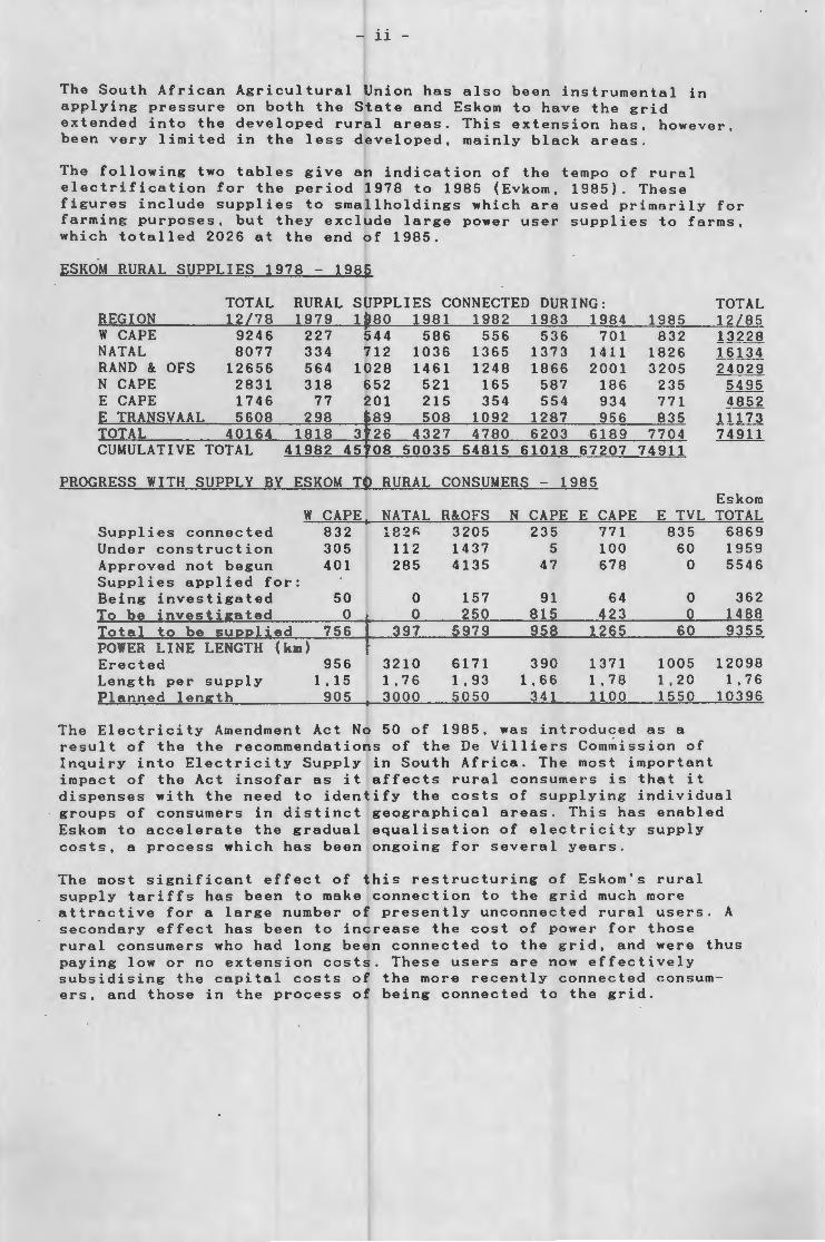
The South African Agricultural Union has also been instrumental in applying pressure on both the State and Eskom to have the grid extended into the developed rural areas. This extension has, however, been very limited in the less developed, mainly black areas.
The following two tables give an indication of the tempo of rural electrification for the period 1978 to 1985 (Evkom, 1985). These figures include supplies to smallholdings which are used primarily for farming purposes, but they exclude large power user supplies to farms, which totalled 2026 at the end of 1985.
ESKOM RURAL SUPPLIES 1978 - 1985
TOTAL RURAL SUPPLIES CONNECTED DURING: TOTAL ~R~E~G~I~O~N------~1~2~/~7~8~~1~9~7~9~~1~9~8~0~-1~9~8~1--~1~9~8~2--~1~9~8~3--~1~9~8~4~21~9~8~5~~1~2~ W CAPE 9246 227 544 586 556 536 701 832 1~~~ NATAL 8077 334 712 1036 1365 1373 1411 1826 16134 RAND & OFS 12656 564 1028 1461 1248 1866 2001 3205 240~
N CAPE 2831 318 652 521 165 587 186 235 ~495
E CAPE 1746 77 201 215 354 554 934 771 4852 E TRANSVAAL 5608 298 589 508 1092 1287 956 835 11173 TOTAL 40164 1818 3726 4327 4780 6203 6189 7704 74911 CUMULATIVE TOTAL 41982 45708 50035 54815 61018 67207 74911
PROGRESS WITH SUPPLY BY ESKOM TO RURAL CONSUMERS - 1985
W CAPE Supplies connected Under construction Approved not begun Supplies applied for: Being investigated To be investigated Total to be supplied POWER LINE LENGTH (km) Erected Length per supply Planned length
832 305 401
50 0
756
956 1. 15
905
NATAL 1821;
112 285
0 0
397
3210 1,76 3000
R&OFS 3205 1437 4135
157 250
5979
6171 1,93 5050
N CAPE 235
5 47
91 815 958
390 1,66
341
E CAPE 771 100 678
64 423
1265
1371 1 . 78 1100
E TVL 835
60 0
0 0
60
1005 1,20 1550
Eskom TOTAL
6869 1959 5546
362 1488 9355
12098 1,76
10396
The Electricity Amendment Act No 50 of 1985, was introduced as a result of the the recommendations of the De Villiers Commission of Inquiry into Electricity Supply in South Africa. The most important impact of the Act insofar as it affects rural consumers is that it dispenses with the need to identify the costs of supplying individual groups of consumers in distinct geographical areas. This has enabled Eskom to accelerate the gradual equalisation of electricity supply costs, a process which has been ongoing for several years.
The most significant effect of this restructuring of Eskom's rural supply tariffs has been to make connection to the grid much more attractive for a large number of presently unconnected rural users. A secondary effect has been to increase the cost of power for those rural consumers who had long been connected to the grid, and were thus paying low or no extension costs. These users are now effectively subsidising the capital costs of the more recently connected consumers, and those in the process of being connected to the grid.
- iii -
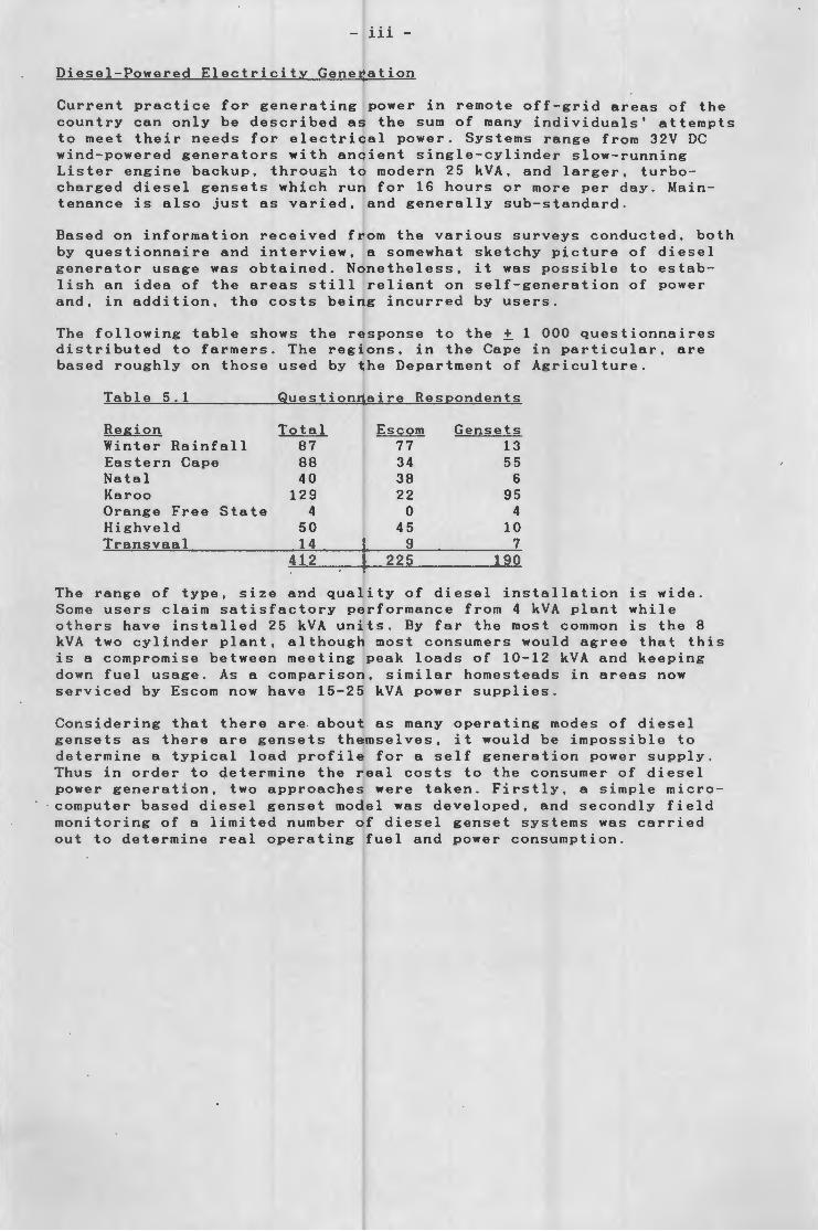
Diesel-Powered Electricity Generation
Current practice for generating power in remote off-grid areas of the country can only be described as the sum of many individuals' attempts to meet their needs for electrical power. Systems range from 32V DC wind-powered generators with ancient single-cylinder slow-running Lister engine backup, through to modern 25 kVA, and larger, turbocharged diesel gensets which run for 16 hours or more per day. Maintenance is also just as varied, and generally sub-standard.
Based on information received from the various surveys conducted, both by questionnaire and interview, a somewhat sketchy picture of diesel generator usage was obtained. Nonetheless, it was possible to establish an idea of the areas still reliant on self-generation of power and, in addition, the costs being incurred by users.
The following table shows the response to the ± 1 000 questionnaires distributed to farmers. The regions, in the Cape in particular, are based roughly on those used by the Department of Agriculture.
Table 5.1 Questionnaire Respondents
Region Total Esc om Gensets Winter Rainfall 87 77 13 Eastern Cape 88 34 55 Natal 40 38 6 Karoo 129 22 95 Orange Free State 4 0 4 Highveld 50 45 10 Transvaal 14 9 7
412 225 190
The range of type, size and quality of diesel installation is wide. Some users claim satisfactory performance from 4 kVA plant while others have installed 25 kVA units. By far the most common is the 8 kVA two cylinder plant, although most consumers would agree that this is a compromise between meeting peak loads of 10-12 kVA and keeping down fuel usage. As a comparison, similar homesteads in areas now serviced by Escom now have 15-25 kVA power supplies.
Considering that there are about as many operating modes of diesel gensets as there are gensets themselves, it would be impossible to determine a typical load profile for a self generation power supply. Thus in order to qetermine the real costs to the consumer of diesel power generation, two approaches were taken. Firstly, a simple microcomputer based diesel genset model was developed, and secondly field monitoring of a limited number of diesel genset systems was carried out to determine real operating fuel and power consumption.
- iv -
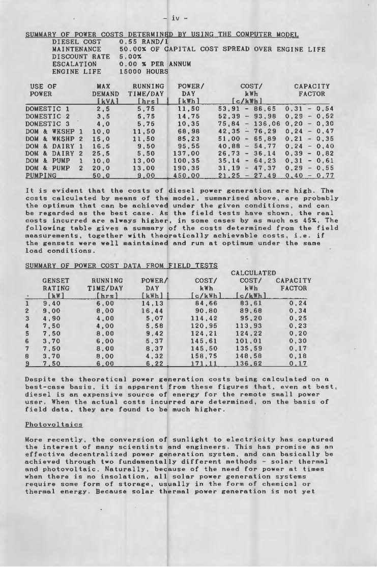
SUMMARY OF POWER COSTS DETERMINED BY USING THE COMPUTER MODEL 0.55 RAND/1 DIESEL COST
MAINTENANCE DISCOUNT RATE ESCALATION ENGINE LIFE
50.00% OF CAPITAL COST SPREAD OVER ENGINE LIFE 5.00%
USE OF MAX POWER DEMAND
[kVA] DOMESTIC 1 2,5 DOMESTIC 2 3,5 DOMESTIC 3 4,0 DOM & WKSHP 1 10,0 DOM & WKSHP 2 15,0 DOM & DAIRY 1 16,5 DOM & DAIRY 2 25,5 DOM & PUMP 1 10,0 DOM & PUMP 2 20,0 PUMPING 50 0
0.00 % PER ANNUM 15000 HOURS
RUNNING POWER/ TIME/DAY DAY
[hrs] [kWh] 5,75 11,50 5,75 14,75 5,75 10,35
11,50 68,98 11,50 85,23
9,50 95,55 5,50 137,00
13,00 100,35 13,00 190,35
9 00 450 00
COST/ CAPACITY kWh FACTOR
[cLkWh] 53,91 - 86,65 0,31 - 0,54 52,39 - 93,98 0,29 - 0,52 75,84 - 136,06 0,20 - 0,30 42,35 - 76,29 0,24 - 0,47 51,00 - 65,89 0,21 - 0,35 40,88 - 54,77 0,24 - 0,40 26,73 - 36. 14 0,39 - 0,82 35,14 - 64,23 0,31 - 0,61 31,19 - 47,37 0,29 - 0,55 21 25 - 27 49 0 40 - 0 77
It is evident that the costs of diesel power generation are high . The costs calculated by means of the model, summarised above, are probably the optimum that can be achieved under the given conditions, and can be regarded as the best case. As the field tests have shown, the real costs incurred are always higher, in some cases by as much as 45%. The following table gives a summary of the costs determined from the field measurements, together with theoretically achievable costs, i.e . if the gensets were well maintained and run at optimum under the same load conditions.
SUMM ARY OF POWER COST DATA FROM FIELD TESTS CALCULATED
GENSET RUNNING POWER/ COST/ COST/ CAPACITY RATING TIME/DAY DAY kWh kWh FACTOR
[kW] [hrs] [kWh] [cLkWh] [cLkWh] 1 9,40 6,00 14,13 84,66 83,61 0,24 2 9,00 8,00 16,44 90,80 89,68 0,34 3 4,90 4,00 5,07 114,42 95,20 0,25 4 7,50 4,00 5,58 120,95 113,93 0,23 5 7,50 8,00 9,42 124,21 124,22 0,20 6 3,70 6,00 5,37 145,61 101,01 0,30 7 7,50 8,00 8,37 145,50 135,59 0. 17 8 3,70 8,00 4,32 158,75 148,58 0. 18 9 7 50 6 00 6 22 171 11 136 62 0 17
Despite the theoretical power generation costs being calculated on a best-case basis, it is apparent from these figures that, even at best, diesel is an expensive source of energy for the remote small power user. When the actual costs incurred are determined, on the basis of field data, they are found to be much higher.
Photovoltaics
More recently, the conversion of sunlight to electricity has captured the interest of many scientists and engineers. This has promise as an effective decentralized power generation system, and can basically be achieved through two fundamentally different methods - solar thermal and photovoltaic . Naturally, because of the need for power at times when there is no insolation, all solar power generation systems require some form of storage, usually in the form of chemical or thermal energy . Because solar thermal power generation is not yet
- v -
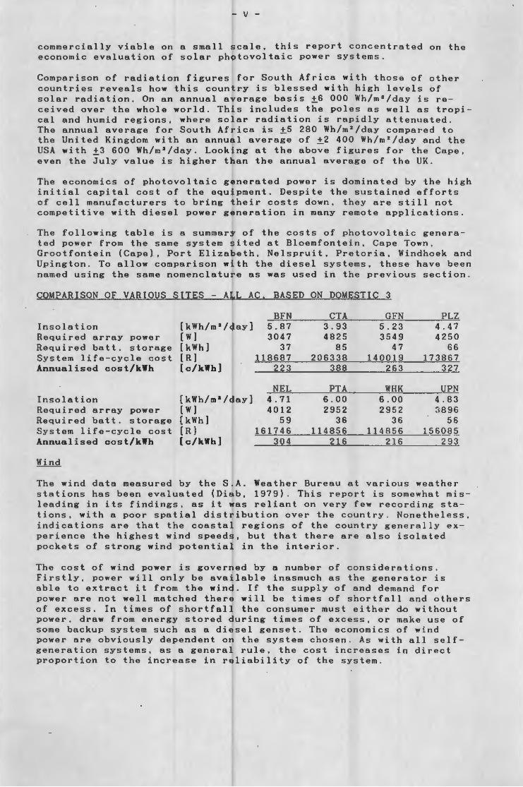
commercially viable on a small scale, this report concentrated on the economic evaluation of solar photovoltaic power systems.
Comparison of radiation figures for South Africa with those of other countries reveals how this country is blessed with high levels of solar radiation. On an annual average basis ±6 000 Wh/m 2 /day is received over the whole world. This includes the poles as well as tropical and humid regions, where solar radiation is rapidly attenuated. The annual average for South Africa is ±5 280 Wh/m 2 /day compared to the United Kingdom with an annual average of ±2 400 Wh/m 2 /day and the USA with ±3 600 Wh/m 2 /day. Looking at the above figures for the Cape, even the July value is higher than the annual average of the UK.
The economics of photovoltaic generated power is dominated by the high initial capital cost of the equipment. Despite the sustained efforts of cell manufacturers to bring their costs down, they are still not competitive with diesel power generation in many remote applications.
The following table is a summary of the costs of photovoltaic generated power from the same system sited at Bloemfontein, Cape Town, Grootfontein (Cape}, Port Elizabeth, Nelspruit, Pretoria, Windhoek and Upington. To allow comparison with the diesel systems, these have been named using the same nomenclature as was used in the previous section .
COMPARISON OF VARIOUS SITES - ALL AC, BASED ON DOMESTIC 3
Insolation Required array power Required batt. storage System life-cycle cost Annualised cost/kWh
Insolation Required array power Required batt. storage System life-cycle cost Annualised cost/kWh
[kWh/m 2 /day] [ w] (kWh] [ R 1 [c/kWh]
[kWh/m 2 /day] [ w 1 (kWh] [ R 1 [c/kWh]
BFN CTA GFN PLZ 5.87 3.93 5.23 4.47 3047 4825 3549 4250
37 85 47 66 ~1~1=8=6=8~7--~2~0~6~3~3~8~~1~4~0019 173867 --~2~2~3~-----3~8~8 ______ ~2~6~3~-----=3~2
~N~E~L ______ ~P~T~A~----~W~H~~K~ ____ yPN 4.71 6.00 6.00 4.83 4012 2952 2952 ~896
59 36 36 56 1617 J_~G--~1~1_,_4=8=5=6----"'1"""'1-.:4. 8 56 15 6 Qll R. ---=3~0~4~----~2~1=6 ______ ~2~1~6~----~293
The wind data measured by the S.A. Weather Bureau at various weather stations has been evaluated (Diab, 1979). This report is somewhat misleading in its findings, as it was reliant on very few recording stations, with a poor spatial distribution over the country. Nonetheless, indications are that the coastal regions of the country generally experience the highest wind speeds, but that there are also isolated pockets of strong wind potential in the interior.
The cost of wind power is governed by a number of considerations. Firstly, power will only be available inasmuch as the generator is able to extract it from the wind. If the supply of and demand for power are not well matched there will be times of shortfall and others of excess. In times of shortfall the consumer must either dQ without power, draw from energy stored during times of excess, or make use of some backup system such as a diesel genset. The economics of wind power are obviously dependent on the system chosen . As with all selfgeneration systems, as a general rule, the cost increases in direct proportion to the increase in reliability of the system.
- vi -
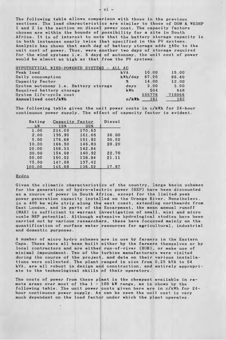
The following table allows comparison with those in the previous sections. The load characteristics are similar to those of DOM & WKSHP 1 and 2 in the section on diesel power cost. The capacity factors chosen are within the bounds of possibility for a site in South
. Africa. It is of interest to note that the battery storage capacity is in both instances nearly twice that specified in the PV systems. Analysis has shown that each day of battery storage adds ±40c to the unit cost of power. Thus, were another two days of storage required for the wind systems i . e. 5 days of autonomy, the unit cost of power would be almost as high as that from the PV systems .
HYPOTHETICAL WIND-POWERED SYSTEMS - ALL AC Peak load kVA 10 . 00 15.00 Daily consumption kWh/day 67.20 86.40 Capacity Factor % 14.00 12.00 System autonomy i.e. Battery storage days 3 . 00 3.00 Required battery storage kWh 504 648 System life-cycle cost 555776 718066 Annualised cost/kWh c/kWh 161 162
The following table gives the unit power costs in c/kWh for 24-hour continuous power supply. The effect of capacity factor is evident.
Rating CaEacit;y: Factor Diesel kW 15% 30%
1. 00 214.09 170.63 2.00 195.95 161.05 36 . 00 5.00 176.68 151.92 30.50
10.00 166.50 146.83 28.20 20.00 158.53 142.84 30 . 00 154.68 · 140.92 22.70 50.00 150.52 138.84 21.11 75.00 147.68 137.42
100.00 145.89 136.52 17.97
Hydro
Given the climatic characteristics of the country, large basin schemes for the generation of hydro-electric power (HEP) have been discounted as a source of power in South Africa, except for the limited peak power generation capacity installed on the Orange River. Nonetheless, in a 400 km wide strip along the east coast, extending northwards from East London, and in parts of the Escarpment, the mean annual runoff (MAR) is sufficient to warrant investigation of small, mini and micro scale HEP potential. Although extensive hydrological studies have been carried .out by various researchers, these have focussed mainly on the quantification of surface water resources for agricultural, industrial and domestic purposes.
A number of micro hydro schemes are in use by farmers in the Eastern Cape. These have all been built either by the farmers themselves or by local contractors and are either run-of-river (ROR), or make use of minimal impoundment. Two of the turbine manufacturers were visited during the course of the project, and data on their various installations were collected. The plant ranged in size from 0,25 kVA to 54 kVA, are all robust in design and construction, and entirely appropriate to the technological skills of their operators.
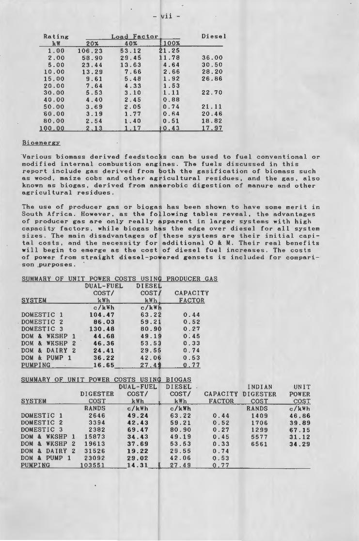
The costs of power from these plant is the cheapest available in remote areas over most of the 1 - 100 kW range, as is shown by the following table. The unit power costs given here are in c/kWh for 24-hour continuous power supply. As can be seen the unit cost is very much dependent on the load factor under which the plant operates.
----
- vii -
Rating Load Factor Diesel kW 20% 40% 100%
1. 00 106.23 53.12 21.25 2.00 58.90 29.45 11.78 36.00 5.00 23.44 13.63 4.64 30.50
10.00 13.29 7.66 2.66 28 . 20 15 . 00 9.61 5.48 1. 92 26.86 20.00 7.64 4.33 1. 53 30.00 5.53 3.10 1.11 22.70 40.00 4 . 40 2.45 0.88 50.00 3.69 2.05 0.74 21. 11 60.00 3.19 1. 77 O . R4 20.46 80.00 2.54 1. 40 0.51 18.82
100.00 2.13 1.17 0 . 43 17.97
Bioenerg;y
Various biomass derived feedstocks can be used to fuel conventional or modified internal combustion engines. The fuels discussed in this report include gas derived from both the gasification of biomass such as wood, maize cobs and other agricultural residues, and the gas, also known as biogas, derived from anaerobic digestion of manure and other agricultural residues.
The use of producer gas or biogas has been shown to have some merit in South Africa. However, as the following tables reveal, the advantages of producer gas are only really apparent in larger systems with high capacity factors, while biogas has the edge over di e sel for all system si z es. The main disadvantages of these systems are their initial capita l costs, and the necessity for additional 0 & M. Their real benefits will begin to emerge as the cost of diesel fuel increases. The costs of power from straight diesel-powered gensets is included for compari-son .Purposes.
§.lli\1 MARY OF UNIT POWER COSTS USING PRODUCER GAS DUAL-FUEL DIESEL
COST/ COST/ CAPACITY SYSTEM kWh kWh FACTOR
c/kWh c/kWh DOMESTIC 1 104.47 63.22 0.44 DOMESTIC 2 86.03 59.21 0.52 DOMESTIC 3 130.48 80.90 0 . 27 DOM & WKSHP 1 44.68 49.19 0.45 DOM & WKSHP 2 46.36 53.53 0.33 DOM & DAIRY 2 24.41 29.55 0.74 DOM & PUMP 1 36.22 42.06 0.53 PUMPING 16.65 27.49 0 . 77
SUMMARY OF UNIT POWER COSTS USING BIOGAS DUAL-FUEL DIESEL INDIAN UNIT
DIGESTER COST/ COST/ CAPACITY DIGESTER POWER SYSTEM COST kWh kWh FACTOR COST COQI
RANDS c/kWh c/kWh RANDS c/kWh DOMESTIC 1 2646 49 . 24 63 . 22 0 . 44 1409 46.86 DOMESTIC 2 3394 42.43 59.21 0.52 1706 39.89 DOMESTIC 3 2382 69.47 80.90 0.27 1299 67.15 DOM & WKSHP 1 15873 34.43 49 . 19 0.45 5577 31.12 DOM & WKSHP 2 19613 37.69 53.53 0.33 6561 34.29 DOM & DAIRY 2 31526 19.22 29.55 0.74 DOM & PUMP 1 23092 29.02 42 . 06 0.53 PUMPING 103551 14.31 27.49 0.77

viii
Hybrids
In many remote areas the levels of available power from an alternate resource such as solar radiation, wind or water may be insufficient to meet the full needs of the consumer. In other cases the cost of the equipment needed to meet the full power needs at desired level of reliability may be prohibitively high . To overcome these problems, the consumer should consider the use of an hybrid power generation system making use of a combination of power sources, exploiting the strong and avoiding the ~eak points of the technologies available.
Clearly, there are no easy rules to follow in selecting an autonomous power system. Almost every application requires careful analysis. This involves the examination of the energy resource to be used, investigation of the competitive technologies, and the evaluation of the total costs over the lifetime of the system. A few hybrid combinations are PV-Diesel, Wind-Diesel and the genset-plus, which combines a diesel genset with battery storage.
Ancillary Equipment
Given the nature of remote area power supply systems, and in particular, those using renewable sources of energy, many such systems require .ancillary equipment of various forms and degrees of sophistication. This can basically be divided into two groups, energy storage equipment and power conditioning equipment. Given its significance in alternative power supply systems, energy storage is dealt with in some detail in the report.
Conclusion
In conclusion, it is hoped that this report highlights some of the potential for the use of alternative power generation technology in South Africa. It should also be stressed that South Africa with its relatively sophisticated manufacturing industry, is well placed to develop and produce power generation equipment appropriate to the needs of rural communities.
- ix -
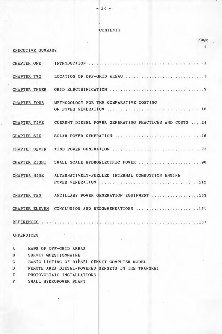
CONTENTS
EXECUTIVE SUMMARY
CHAPTER ONE INTRODUCTION ............... .... ...... ... .. .. ........... . 1
CHAPTER TWO LOCATION OF OFF-GRID AREAS ................ .... . ... .. .... 3
CHAPTER THREE GRID ELECTRIFICATION ............... ............... . ... .. 9
CHAPTER FOUR METHODOLOGY FOR THE COMPARATIVE COSTING
OF POWER GENERATION ......................... . .. . .. ..... 18
CHAPTER FIVE CURRENT DIESEL POWER GENERATING PRACTICES AND COSTS .... 24
CHAPTER SIX SOLAR POWER GENERATION ................... . ............. 46
CHAPTE» SEVEN WIND POWER GENERATION ............... ... .. .. ........... . 73
CHAPTER EIGHT SMALL SCALE HYDROELECTRIC POWER ...... .... .. .. ..... . . ... 90
CHAPT~R NINE ALTERNATIVELY-FUELLED INTERNAL COMBUST ION ENGINE
POWER GENERATION ............................. . ........ 112
CHAPTER TEN ANCILLARY POWER GENERATION EQUIPMENT ... .. . .. .. ....... . 132
CHAPTER ELEVEN CONCLUSION AND RECOMMENDATIONS ...... .... . ......... .... 151
REFERENCES ............................................................ 15 7
APPENDICES
A MAPS OF OFF-GRID AREAS
B SURVEY QUESTIONNAIRE
C BASIC LISTING OF DIESEL GENSET COMPUTER MODEL
D REMOTE AREA DIESEL-POWERED GENSETS IN THE TRANSKEI
E PHOTOVOLTAIC INSTALLATIONS
F SMALL HYDROPOWER PLANT
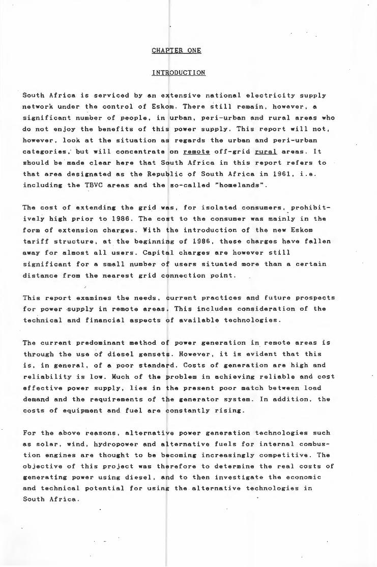
CHAPTER ONE
INTRODUCTION
South Africa is serviced by an extensive national electricity supply
network under the control of Eskom. There still remain, however, a
significant number of people, in urban, peri-urban and rural areas who
do not enjoy the benefits of this power supply. This report will not,
however, look at the situation as regards the urban and peri-urban
categories; but will concentrate on remote off-grid rural areas. It
should be made clear here that South Africa in this report refers to
that area designated as the Republic of South Africa in 1961, i.e.
including the TBVC areas and the so-called "homelands".
The cost of extending the grid was, for isolated consumers, prohibit
ively high prior to 1986. The cost to the consumer was mainly in the
form of extension charges. With the introduction of the new Eskom
tariff structure, at the beginning of 1986, these charges have fallen
away for almost all users. Capital charges are however still
significant for a small number of users situated more than a certain
distance from the nearest grid connection point.
This report examines the needs, current practices and future prospects
for power supply in remote areas. This includes consideration of the
technical and financial aspects of available technologies.
The current predominant method of power generation in remote areas is
through the use of diesel gensets. However, it is evident that this
is, in general, of a poor standard. Costs of generation are high and
reliability is low. Much of the problem in achieving reliable and cost
effective power supply, lies in the present poor match between load
demand and the requirements of the generator system . In addition, the
costs of equipment and fuel are constantly rising.
For the above reasons, alternative power generation technologies such
as solar, wind, hydropower and alternative fuels for internal combus
tion engines are thought to be becoming increasingly competitive. The
objective of this project was therefore to determine the real costs of
generating power using diesel, and to then investigate the economic
and technical potential for using the alternative technologies in
South Africa.

2
KEY QUESTIONS
The key questions can be summarized as follows:
* What are the approximate number, typical energy demands and
geographical locations of off-grid users of diesel generating
sets?
* What are the range of actual operating costs of diesel
generating sets in remote areas?
* What is the range of capital costs and performance character
istics of locally available conventional and alternative power
generation systems, and ancillary equipment?
* What are the comparative lifetime costs of power supplied in
remote areas by stand-alone or hybrid diesel I battery I wind I
photovoltaic and other alternative power generation systems?
* What will the effects of future cost shifts be (particularly
photovoltaic module prices) on the comparative economics of
alternative energy technologies for remote area power supply?
REPORT OUTLINE
The report follows the sequence of the key questions . Chapters Two and
Three deal with the status quo as regards remote area power supply in
as much detail as possible . Subsequent chapters deal with the techni
cal and economic aspects of the alternative power sources available.
It is important to be constantly aware of the site specificity of many
of the renewable energy resources. This factor makes it difficult to
make a thorough comparison of the alternatives, and the reader should
take careful note of the assumptions pertaining to each case.
3
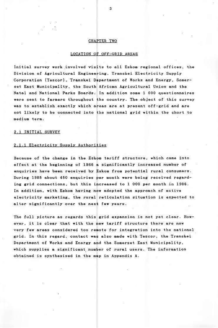
CHAPTER TWO
LOCATION OF OFF-GRID AREAS
Initial survey work involved visits to all Eskom regional offices, the
Division of Agricultural Engineering, Transkei Electricity Supply
Corporation (Tescor), Transkei Department of Works and Energy, Somer
set East Municipal1ty, the South African Agricultural Union and the
Natal and National Parks Boaras. In addition some 1 000 questionnaires
were sent to farmers throughout the country. The object of this survey
was to establish exactly which areas are at present off-grid and are
not likely to be connected into the national grid within the short to
medium term.
2 . 1 INITIAL SURVEY
2.1.1 Electricity Supply Authorities
Because of the change in the Eskom tariff structure, which came into
effect at the beginning of 1986 a significantly increased number of
enquiries have been received by Eskom from potential rural consumers.
During 1985 about 450 enquiries per month were being received regard
ing grid connections, but this increased to 1 000 per month in 1986.
In addition, with Eskom having now adopted the approach of active
electricity marketing, the rural reticulation situation is expected to
alter significantly over the next few years.
The full picture as regards this grid expansion is not yet clear. How
ever, it is clear that with the new tariff structure there are now
very few areas considered too remote for integration into the national
grid. In this regard, contact was also made with Tescor, the Transkei
Department of Works and Energy and the Somerset East Municipality,
which supplies a significant. number of rural users. The information
obtained is synthesised in the map in Appendix A.

4
2.1.2 Agricultural Groupings
The Department of Agriculture was helpful in making contact with
commercial farmers 1 • In order to distribute questionnaires, the well
developed network of study groups was used as the point of contact.
The extension officers in the various regions made this possible. In
addition appeals for information were also made through the Farmer ' s
Weekly, Landbouweekblad, the SABC and various newspapers . The response
from these sources was not that encouraging, resulting in about 20 of
the replies received.
Because extra photocopies of the questionnaire were ·made by extension
officers, it is difficult to estimate exactly how many were finally
distributed. Based on the number of study groups contacted, and their
average size, 1 000 has been taken as the final number of question
naires. Of these 412 were returned, which, in the Energy Research
Institute's (ERI) experience, is a better than normal response .
As can be seen from the sample questionnaire (Appendix B), details
asked for included broader aspects of energy utilisation. Some of
these additional data have already been used in another ERI report
(Eberhard, 1986). Obviously of interest in this report are the data
pertaining to power generation. After careful screening, these data
were statistically analysed on the UCT Univac mainframe computer.
Because filling out of the questionnaires was unsupervised, the quali
ty of the data received was extremely variable. This meant that they
had to be carefully screened prior to processing, and even then the
results obtained must be treated critically . The variability in the
quality of data itself is significant, in that it reveals the somewhat
varying degree of concern shown by power users towards the costs they
face. This is of particular interest with respect to those respondents
involved in self-generation of power.
Despite the poor data quality, valuable information was received on
the actual costs being incurred through diesel generation of electri
city.
1 It was assumed in this study that for all practical purposes,
black farmers do not have access to electricity
5
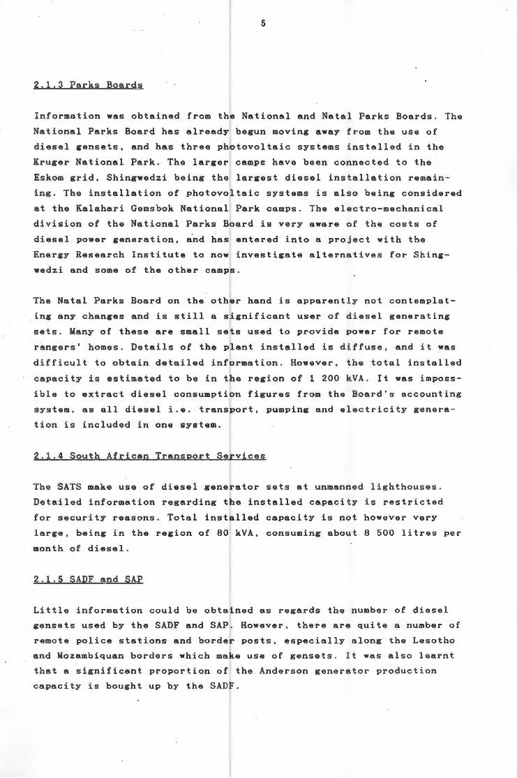
2.1.3 Parks Boards
Information was obtained from the National and Natal Parks Boards. The
National Parks Board has already begun moving away from the use of
diesel gensets, and has three photovoltaic systems installed in the
Kruger National Park. The larger camps have been connected to the
Eskom grid, Shingwedzi being the largest diesel installation remain
ing. The installation of photovoltaic systems is also being considered
at the Kalahari Gemsbok National Park camps. The electro-mechanical
division of the National Parks Board is very aware of the costs of
diesel power generation, and has entered into a project with the
Energy Research Institute to now investigate alternatives for Shing
wedzi and some of the other camps.
The Natal Parks Board on the other hand is apparently not contemplat
ing any changes and is still a significant user of diesel generating
sets. Many of these are small sets used to provide power for remote
rangers' homes. Details of the plant installed is diffuse, and it was
d i fficult to obtain detailed information. However , the total installed
capacity is estimated to be in the region of 1 200 kVA . It was imposs
ib l e to extract diesel consumption figures from the Board's accounting
system , as all diesel i.e. transport, pumping and electricity genera
t i on is included in one system.
2 .1 .4 South African Transport Services
The SATS make use of diesel generator sets at unmanned lighthouses.
De t ailed information regarding the installed capacity is restricted
fo r security reasons. Total installed capacity is not however very
lar ge, being in the region of 80 kVA, consuming about 8 500 litres per
month of diesel .
2 .1. 5 SADF and SAP
Lit tle information could be obtained as regards the number of diesel
gensets used by the SADF and SAP . However, there are quite a number of
remote police stations and border posts, especially along the Lesotho
and Mozambiquan borders which make use of gensets. It was also learnt
that a significant proportion of the Anderson generator production
capacity is bought up by the SADF .
6
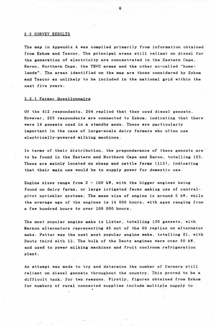
2.2 SURVEY RESULTS
The map in Appendix A was compiled primarily from information obtained
from Eskom and Tescor. The principal areas still reliant on diesel for
the gen~ration of electricity are concentrated in the Eastern Cape ,
Karoo, Northern Cape, the TBVC areas and the other so-called "home
lands". The areas identified on the map are those considered by Eskom
and Tescor as unlikely to be included in the national grid within the
next five years .
2.2.1 Farmer Questionnaire
Of the 412 respondents, 204 replied that they used diesel gense ts.
However, 225 respondents are connected to Eskom, indicating that there
were 14 gensets used in a standby mode. These are particularly
important in the case of large-scale dairy farmers who often use
electrically-powered milking machines .
In terms of their distribution, the preponderance of these gensets are
to be found in the Eastern and Northern Cape and Karoo, totalling 153 .
These are mainly located on sheep and cattle farms (113), indicating
that their main use would be to supply power for domestic use .
Engine sizes range from 2 - 100 kW, with the bigger engines being
found on dairy farms, or large irrigated farms making use of central
pivot sprinkler systems. The mean size of engine is around 5 kW, while
the average age of the engines is 14 000 hours , with ages ranging from
a few hundred hours to over 100 000 hours .
The most popular engine make is Lister, totalling 130 gensets, with
Markon alternators representing 45 out of the 60 replies on alternator
make. Petter was the next most popular engine make , totalling 21, with
Deutz third with 13. The bulk of the Deutz engines were over 50 kW,
and used to power milking machines and fruit coolroom refrigeration
plant.
An attempt was made to try and determine the number of farmers still
reliant on diesel gensets throughout the country . This proved to be a
difficult task, for two reasons. Firstly, figures obtained from Eskom
for numbers of rural connected supplies include multiple supply to
7
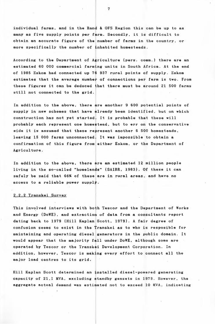
individual farms, and in the Rand & OFS Region this can be up to as
many as five supply points per farm. Secondly, it is difficult to
obtain an accurate figure of the number of farms in the country, or
more specifically the number of inhabited homesteads.
According to the Department of Agriculture (pers. comm.) there are an
estimated 60 000 commercial farming units in South Africa. At the end
of 1985 Eskom had connected up 76 937 rural points of supply. Eskom
estimates that the average riumber of connections per farm is two. From
these figures it can be deduced that there must be around 21 500 farms
still not connected to the grid.
In addition to the above, there are another 9 600 potential points of
supply in new schemes that have already been identified, but on which
construction has not yet started. It is probable that these will
probably each represent one homestead, but to err on the conservative
side it is assumed that these represent another 6 500 homesteads,
leaving 15 000 farms unconnected. It was impossible to obtain a
confirmation of this figure from either Eskom, or the Department of
Agriculture.
In addition to the above, there are an estimated 12 million people
living in the so-called "homelands" (SAIRR, 1983). Of these it can
safely be said that 66% of these are in rural areas, and have no
access to a reliable power supply.
2.2 . 2 Transkei Survey
This involved interviews with both Tescor and the Department of Works
and Energy (DoWE), and extraction of data from a consultants report
dating back to 1979 (Hill Kaplan Scott, 1979) . A fair degree of
confusion seems to exist in the Transkei as to who is resposible for
maintaining and operating diesel generators in the public domain . It
would appear that the majority fall under DoWE, although some are
operated by Tescor or the Transkei Development Corporation. In
addition, however, Tescor is making every effort to connect all the
major load centres to its grid.
Hill Kaplan Scott determined an installed diesel-powered generating
capacity of 21,1 MVA, excluding standby gensets in 1979 . However, the
aggregate actual demand was estimated not to exceed 10 MVA, indicating

8
a more than 100% overcapacity. The diesel consumption was estimated to
be of the order of 10 million 1/yr.
Since that report was written, Tescor has extended its grid quite
significantly to pick up many of the larger loads . In addition, many
smaller loads have been supplied in the process. Plans for the next
five years are such that there ~ill be virtu•lly no significant load
centres in the form of towns, hospitals, sawmills, tea factories and
other remotely sited industries remaining to be connected . There will
be a few schools and remote clinics still unconnected. Appendix D con
tains a list of the significant loads still served by diesel gensets
in 1986.
2.2.3 Other "homelands"
Through discussions with administrative personnnel and consulting
engineers involved in these areas, and Eskom personnel, i t was
established that very little in terms of rural electrificat i on was
being done in these areas. The major load centres , i . e . towns and
industrial areas are all either already supplied from the grid, or are
planned to be connected in the next five years .
2.3 CONCLUSION
I t is apparent that there are still fairly significant areas of the
country reliant on self-generation of power, or without any power
generation facilities. Current off-grid power users can be categorised
as follows:
Commercial farmers
"Homeland" areas
- Clinics
- Schools
- ' Industries
- Hotels
- Small businesses
Small demands
- Telecommunications
- Navigational aids
9
CHAPTER THREE
GRID ELECTRIFICATION
In the past, many small towns and villages generated their own power,
making use of diesel generators. Subsequent to the petroleum price
increase of 1973 and because of continued escalating fuel costs,
pressure was placed on Eskom to connect them to the national grid.
This has resulted in significant extensions of the grid over the last
decade, to the extent that there are now virtually no towns or
villages outside the "homelands" which do not have Eskom power. This
extension of the grid to these settlements has made it possible to now
supply many remote rural consumers located along the route of the
power lines .
The South African Agricultural Union has also been instrumental in
applying pressure on both the State and Eskom to have the grid
extended into the developed rural areas. This extension has, however,
been very limited in the less developed, mainly black areas.
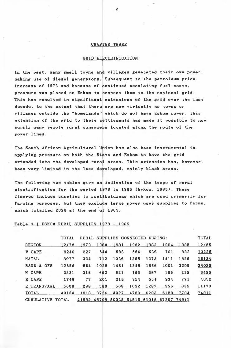
The following two tables give an indication of the tempo of rural
electrification for the period 1978 to 1985 (Evkom, 1985). These
figures include supplies to smallholdings which are used primarily for
farming purposes, but they exclude large power user supplies to farms,
which totalled 2026 at the end of 1985.
Table 3.1 ESKOM RURAL SUPPLIES 1978 - 1985
TOTAL RURAL SUPPLIES CONNECTED DURING: TOTAL
REGION 12L78 1979 1980 1981 1982 1983 1984 1985 12L85
W CAPE 9246 227 544 586 556 536 701 832 13228
NATAL 8077 334 712 1036 1365 1373 1411 1826 16134
RAND &. OFS 12656 564 1028 1461 1248 1866 2001 3205 24029
N CAPE 2831 318 652 521 165 587 186 235 5495
E CAPE 1746 77 201 215 354 554 934 771 4852
E TRANSVAAL 5608 298 589 508 1092 1287 956 835 11173
TOTAL 40164 1818 3726 4327 4780 6203 6189 7704 74911
CUMULATIVE TOTAL 41982 45708 50035 54815 61018 67207 74911
10
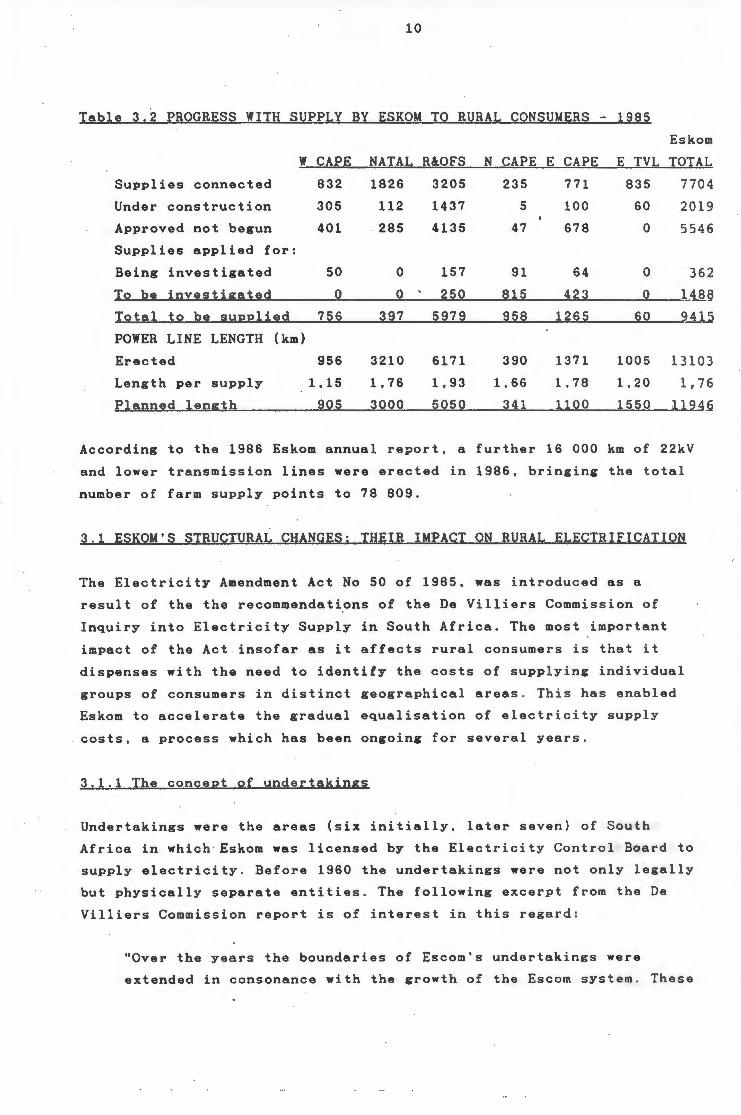
Table 3.2 PROGRESS WITH SUPPLY BY ESKOM TO RURAL CONSUMERS - 1985
Eskom
w CAPE NATAL R&.OFS N CAPE E CAPE E TVL TOTAL
Supplies connected 832 1826 3205 235 771 835 7704
Under construction 305 112 1437 5 100 60 2019
Approved not begun 401 285 4135 47 678 0 5546
Supplies applied for:
Being investigated 50 0 157 91 64 0 362
To be investigated 0 0 250 815 423 0 1~6
Total to be SUEElied 756 397 5979 958 1265 60 9...!1..5
POWER LINE LENGTH (km)
Erected 956 3210 6171 390 1371 1005 13103
Length per supply 1.15 1,76 1,93 1,66 1,78 1,20 1,76
Planned length 905 3000 5050 341 1100 1550 ll9_A_6
According to the 1986 Eskom annual report, a further 16 000 km of 22kV
and lower transmission lines were erected in 1986, bringing the total
number of farm supply points to 78 809.
3.1 ESKOM'S STRUCTURAL CHANGES; THEIR IMPACT ON RURAL ELECTRIFICATION
The Electricity Amendment Act No 50 of 1985, was introduced as a
result of the the recommendations of the De Villiers Commission of
Inquiry into Electricity Supply in South Africa. The most important
impact of the Act insofar as it affects rural consumers is that it
dispenses with the need to identify the costs of supplying individual
groups of consumers in distinct geographical areas . This has enabled
Eskom to accelerate the gradual equalisation of electric i ty supply
costs, a process which has been ongoing for several years.
3.1.1 The conceEt of undertakings
Undertakings were the areas (six initially, later seven) of South
Africa in which Eskom was licensed by the Electricity Control Board to
supply electricity. Before 1960 the undertakings were not only legally
but physically separate entities . The following excerpt from the De
Villiers Commission report is of interest in this regard :
"Over the years the boundaries of Escom's undertakings were
extended in consonance with the growth of the Escom system . These
11
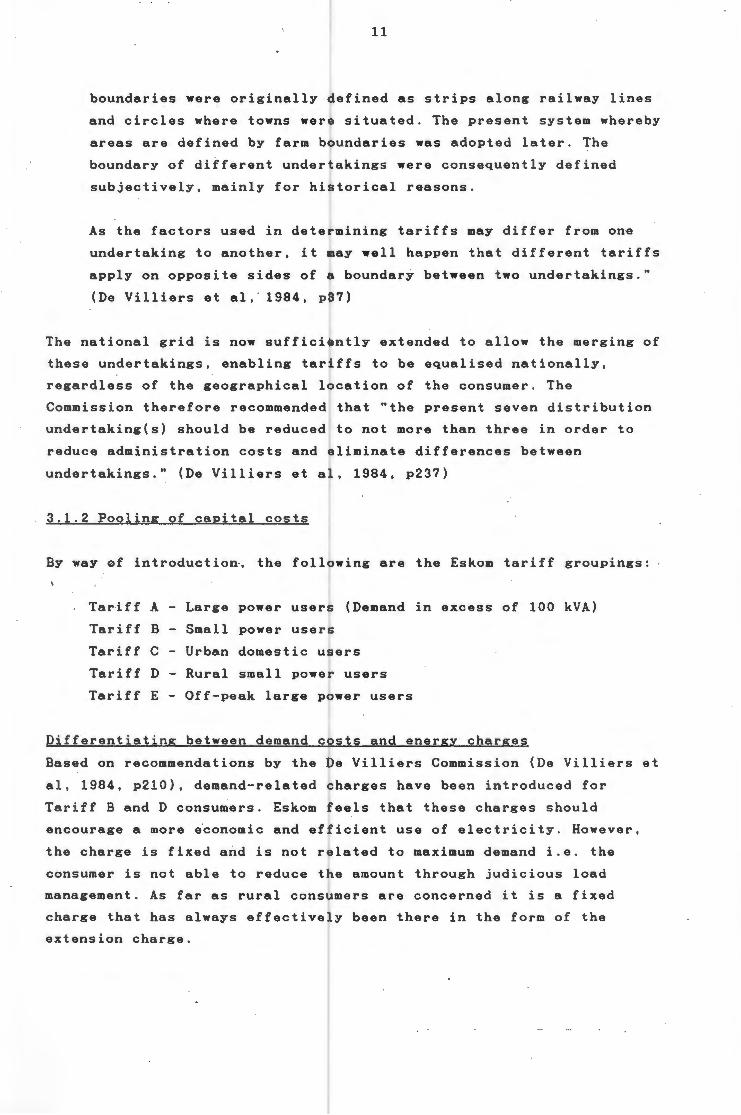
boundaries were originally defined as strips along railway lines
and circles where towns were situated . The present system whereby
areas are defined by farm boundaries was adopted later . The
boundary of different undertakings were consequently defined
subjectively, mainly for historical reasons.
As the factors used in determining tariffs may differ from on~
undertaking to another, it may well happen that different tariffs
apply on opposite sides of a boundary between two undertakings."
(De Villiers et al, · 1984, p37)
The national grid is now sufficiently extended to allow the merging of
these undertakings, enabling tariffs to be equalised nationally,
regardless of the geographical location of the consumer. The
Commission therefore recommended that "the present seven distribution
undertaking(s) should be reduced to not more than three in order to
reduce administration costs and eliminate differences between
undertakings." (De Villiers et al, 1984, p237)
3.1 . 2 Pooling of capital costs
By way af introduction·, the following are the Eskom tariff groupings:
Tariff A Large power users (Demand in excess of 100 kVA)
Tariff B - Small power users
Tariff C - Urban domestic users
Tariff D - Rural small power users
Tariff E - Off-peak large power users
Differentiating between demand costs and energy charges
Based on recommendations by the De Villiers Commission (De Villiers et
al , 1984, p210), demand-related charges have been introduced for
Tariff B and D consumers. Eskom feels that these charges should
encourage a more economic and efficient use of electricity. However,
the charge is fixed and is not r l lated to maximum demand i.e. the I
consumer is not able to reduce the amount through judicious load
management. As far as rural consumers are concerned it is a fixed
charge that has always effectively been there in the form of the
ex t ension charge.
12
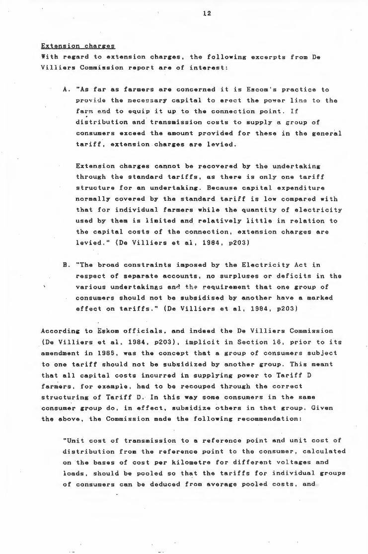
Extension charges
With regard to extension charges, the following excerpts from De
Villiers Commission report are of interest:
A. "As far as farmers are concerned it is Escom ' s practice to
provid e the necessary capital to erect the po~er li ne to the
far m ~nd to equip it up to the connection point. If
distribution and transmission costs to supply a group of
consumers exceed the amount provided for these in the general
tariff, extension charges are levied .
Extension charges cannot be recovered by the undertaking
through the standard tariffs, as there is only one tariff
structure for an undertaking. Because capital expenditure
normally covered by the standard tariff is low compared with
that for individual farmers while the quantity of electricity
used by them is limited and relatively little in relation to
the capital costs of the connection, extension charges are
le~ied." (De Villiers et al, 1984 , p203)
B. "The broad constraints imposed by the Electricity Act in
respect of separate accounts, no surpluses or deficits in the
various undertaking~ and t h~ requirement that one group of
consumers should not be subsidised by another have a marked
effect on tariffs." (De Villiers et al, 1984, p203)
According to Eskom officials, and indeed the De Villiers Commiss i on
(De Villiers et al, 1984, p203), implicit in Section 16 , prior t o i ts
amendment in 1985, was the concept that a group of c onsumers sub j e ct
to one tariff should not be subsidized by another group. This meant
that all capital costs incurred in supplying power to Tariff D
farmers, for example, had to be recouped through the correct
structuring of Tariff D. In this way some consumers in the same
consumer group do, in effect, subsidize others in that group. Given
the above, the Commission made the following recommendation:
"Unit cost of transmission to a reference point and un i t cost of
distribution from the reference point t o the consumer , ca l cu l ated
on the bases of cost per kilometre for different voltages and
loads, should be pooled so that the tariffs for individual groups
of consumers can be deduced from average pooled costs, and
13
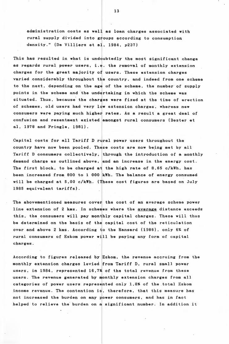
administration costs as wel \ as loan charges associated with
rural supply divided into g f oups according to consumption I
density." (De Villiers et al, 1984, p237)
This has resulted in what is undl ubtedly the most significant change
as regards rural power users, i.e. the removal of monthly extension
charges for the great majority of users. These extension charges
varied considerably throughout the country, and indeed from one scheme
to the next, depending on the age of the scheme, the number of supply
points in the scheme and the undertaking in which the scheme was
situated. Thus, because the charges were fixed at the time of erection
of schemes, old users had very low extension charges, whereas new
consumers were paying much higher rates. As a result a great deal of
confusion and resentment existed amongst rural consumers (Bester et
al, 1978 and Pringle, 1981).
Capital costs for all Tariff D rural power users throughout the
country have now been pooled. These costs are now being met by all
Tariff D consumers collectively, through the introduction of a monthly
demand charge as outlined above, and an increase in the energy cost .
The first block, to be charged at the high rate of 8,65 c/kWh, has
been increased from 800 to 1 000 kWh. The balance of energy consumed
will be charged at 5,00 c/kWh. hese cost figures are based on July
1985 equivalent tariffs).
The abovementioned measures coven the cost of an average scheme power
line extension of 2 kms . In schemes where the average distance exceeds
this, the consumers will pay mon lhly capital charges . These will thus
be determined on the basis of the capital cost of the reticulation
over and above 2 kms. According J o the Hansard (1986), only 6% of
rural consumers of Eskom power wJ 11 be paying any form of capital
charges.
According to figures released by Eskom, the revenue accruing from the
monthly extension charges levied from Tariff D, rural small power
users, in 1984, represented 16,7j of the total revenue from these
users . The revenue generated by monthly extension charges from all
categories of power users represented only 1,8% of the total Eskom
income revenue. The contention is, therefore, that this measure has
not increased the burden on any ower consumers, and has in fact
helped to relieve the burden on a significant number. In addition it
14
has made it attractive for a greater number of rural consumers to be
connected to the grid.
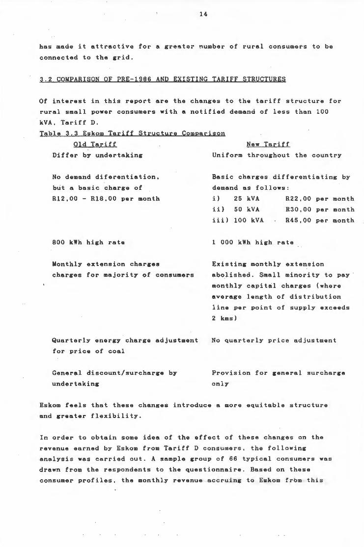
3 . 2 COMPARISON OF PRE-1986 AND EXISTING TARIFF STRUCTURES
Of interest in this report are the changes to the tariff structure for
rural small power consumers with a notified demand of less than 100
kVA, Tariff D.
Table 3.3 Eskom Tariff Structure Comparison
Old Tariff
Differ by undertaking
No demand diferentiation,
but a basic charge of
Rl2,00 - Rl8,00 per month
800 kWh high rate
Monthly extension charges
charges for majority of consumers
Quarterly energy charge adjustment
for price of coal
General discount/surcharge by
undertaking
New Tariff
Uniform throughout the country
Basic charges differentiating by
demand as follows:
i) 25 kVA R22,00 per month
ii) 50 kVA
iii) 100 kVA
R30,00 per month
R45,00 per month
1 000 kWh high rate
Existing monthly extension
abolished. Small minority to pay ·
monthly capital charges (where
average length of distribution
line per point of supply exceeds
2 kms)
No quarterly price adjustment
Provision for general surcharge
only
Eskom feels that these changes introduce a more equitable structure
and greater flexibility.
In order to obtain some idea of the effect of these changes on the
revenue earned by Eskom from Tariff D consumers , the following
analysis was carried out. A sample group of 66 typical consumers was
drawn from the respondents to the questionnaire. Based on these
consumer profiles, the monthly revenue accruing to Eskom from this
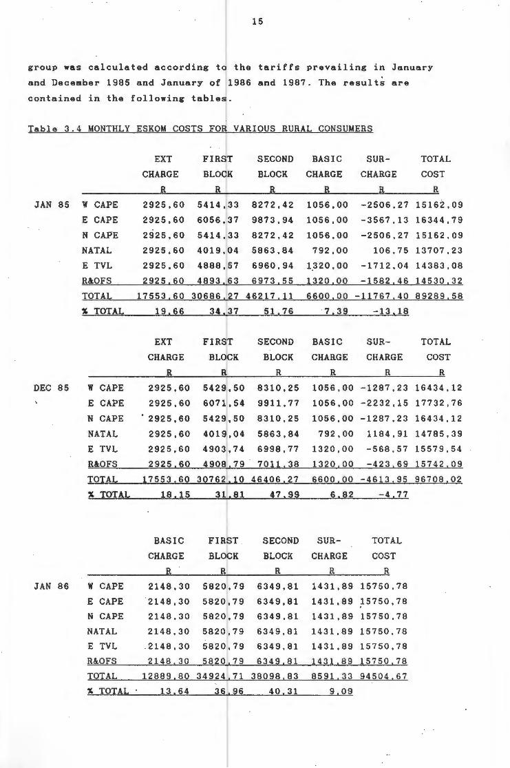
15
group was calculated according to the tariffs prevailing in January
and December 1985 and January of 1986 and 1987. The results are
contained
Table 3.4
JAN 85 W CAPE
E CAPE
N CAPE NATAL
E TVL
R&.OFS
DEC 85
JAN 86
TOTAL
% TOTAL
W CAPE
E CAPE
N CAPE
NATAL E TVL
R&.OFS
TOTAL
% TOTAL
w CAPE
E CAPE
N CAPE NATAL E TVL
R&.OFS TOTAL % TOTAL
EXT
CHARGE
R
2925,60
2925,60
2925,60
2925,60
2925,60
FIRST
BLOCK
R
5414,33
6056,37
5414,33
4019,04
4888,57
RURAL CONSUMERS
SECOND
BLOCK
R
8272,42
9873,94
8272,42
5863,84
6960,94
BASIC
CHARGE
R
1056,00
1056,00
1056,00
792,00
1.320. 00
SUR
CHARGE
R
TOTAL
COST
R
-2506,27 15162,09
-3567,13 16344,79
-2506,27 15162,09
106,75 13707,23
-1712,04 14383,08
2925.60 4893.63 6973.55 1320.00 -1582,46 14530,32
17553,60 30686,27 46217.11
19.66 34.37 51.76
EXT FIRj T SECOND
CHARGE BLOCK BLOCK
R R R
2925,60 5429,50 8310,25
2925,60 6071,54 9911,77
'2925,60 5429,50 8310,25
2925,60 4019,04 5863,84
2925,60 4903,74 6998,77
2925,60 4908,79 7011.38
17553,60 30762.10 46406.27
18.15 31.81 47.99
BASIC FIR T SECOND
CHARGE BLObK BLOCK
R R R
2148,30 5820,79 6349,81
2148,30 5820,79 6349,81
2148,30 5820,79 6349,81
2148,30 5820,79 6349,81
. 2148,30 5820,79 6349,81
2148,30 5820,79 6349,81
12889,80 349241,71 38098,83
13,64 36,96 40,31
6600,00 -11767,40 89289,58
·7' 39
BASIC
CHARGE
R
-13.18
SUR
CHARGE
R
TOTAL
COST
R
1056,00 -1287,23 16434,12
1056,00 -2232,15 17732,76
1056,00 -1287,23 16434,12
792,00 1184,91 14785,39
1320,00 -568,57 15579,54
1320,00 -423,69 15742.09
6600.00 -4613.95 96708,02
6,82 -4,77
SUR- TOTAL
CHARGE COST R R
1431,89 15750,78
1431,89 15750,78
1431,89 15750,78
1431,89 15750,78
1431,89 15750,78
1431,89 15750,78
8591,33 94504,67
9,09
16
BASIC FIRST SECOND SUR- TOTAL
CHARGE BLOCK BLOCK CHARGE COST
JAN 87 w CAPE 2148,30 5820,79 6349 ,. 81 5083 , 21 24405 ,4 6
E CAPE 2148,30 5820,79 6349,81 5083,21 24405,46
N CAPE 2148,30 5820,79 6349,81 5083,21 24405,46
NATAL 2148,30 5820,79 6349,81 5083,21 24405 , 46
E TVL 2148,30 5820,79 6349,81 5083,21 24405,46
R&.OFS 2148,30 5820,79 6349,81 5083,21 24405,46
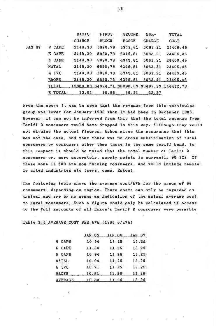
TOTAL 12889,80 34924,71 38098,83 30499,23 146432,70
% TOTAL 13,64 36,96 40,31 32,27
From the above it can be seen that the revenue from this particu l ar
group was lower for January 1986 than it had been in December 1985 .
However, it can not be inferred from this that the total revenue from
Tariff D consumers would have dropped in this way. Although they would
not divulge the actual figures, Eskom gives the assurance that this
was not the case, and that there was no cross-subsidisation of rural
consumers by consumers other than those in the same tariff band . In
this respect it should be noted that the total number of Tariff D
consumers or, more accurately, supply points is currently 90 329. Of
these some 11 500 are non-farming consumers, and would include remote
ly sited industries etc (pers. comm. Eskom).
The following table shows the average cost/kWh for the group of 66
consumers, depending on region. These costs can only be regarded as
typical and are by no means an indication of the actual average cost
to rural consumers. Such a figure could only be calculated if access
to the full accounts of all Eskom's Tariff D consumers were possible .
Table 3.5 AVERAGE COST PER kWh (1985 c/kWh)
JAN 85 JAN 86 JAN 87
w CAPE 10,94 11 '25 13,25
E CAPE 11 '54 11 '25 13,25
N CAPE 10,94 11 '25 13,25
NATAL 10 , 04 11 '25 13,25
E TVL 10,71 11' 25 13 , 25
R&.OFS 10,81 11,25 13,25
AVERAGE 10,83 11,25 13,25
17
The previous table shows an average real increase in unit cost of 4%
from January 1985 to 1986, with ~ significant increase to January 1987
of nearly 18%.
3 . 3 GRID EXTENSION COSTS
The cost per kilometre of power ine varies significantly depending on
its power rating, the terrain ovr r which it passes, the specifications
to which it is constructed, and he contractors who undertake the
work. Figures quoted by engineers from Eskom, Tescor and consultants
vary as widely as from R8 000 to R20 000 per km of 11 kV line. In
addition to this there is the cost of switchgea~ and transformers,
which will of ~ourse be dependenl on the requirements of the consumer.
From the above it is apparent that site specificity, amongst other
factors, will affect the cost of supplying grid based power to a re
mote rural power consumer.
3 . 4 CONCLUSION
The most significant effect of this restructuring of Eskom's rural
supply tariffs has been to make bonnection to the grid much more
attractive for a large number of presently unconnected users. A secon-
. dary effect has been to increase the cost of power for those rural
consumers who had long been conn ! cted to the grid, and were thus pay
ing low or no extension costs~ Tf ese users are now effectively subsi
dising the capital costs of the more recently connected consumers, and
those in the process of being cohnected to the grid .
18
CHAPTER FOUR
METHODOLOGY FOR THE COMPARATIVE COSTING OF POWER GENERATION
Many consumers of self-generated power are unaware of the true cos t of
the electricity they are generating. Expenses seen by the operator of
a diesel genset, for example, are usually limited to the capital cost
of the installation, the monthly fuel bills and infrequent repair
bills, usually at breakdown. Little, if any connection is made between
these cash payments and the electricity consumption. If costs per kWh
are calculated in such situations, it is usually on the often erron
eous assumption that the capacity factor for the genset is close to
unity. In most instances, the capacity factor is far less and un i t
costs of generation are high. For the above reasons it is imp~rtant to
calculate the cost of electricity over the life of the installat i on.
In formulating typical systems for comparison in the report , i t i s
assumed that a fixed common peak power and annual demand are to be
met. Power generated above the amount considered necessary is no t
granted financial credit. Likewise systems not capable of meeting the
demand criteria are not considered. The principle of working to a
fixed demand requirement differs from the practice of calculating
electricity costs . on the basis of net power generated. For remote area
users, the method of working to a fixed demand most closely matches
the real situation, and eliminates the use of low-cost make-shift
systems . It also does not favour, for example , wi nd generator s located
in windy areas where excess power may be available .
In the report some adjustments will be made to this basic approach for
particular systems, to bring the annual costing as close as possible
to actual practice . These modifications will be detailed under the
relevant section. The principal assumptions and any minor adjustments
are discussed below. Particular note must be taken of the methodology
us~d and assumptions made in the costing technique, as the resultant
cost of electricity is very dependent upon them.
4.1 COSTING METHODOLOGY
Essential to the consideration of power generation alternatives is
their cost competttiveness relative to one another . Before a fair com
parison can be made , the true unit cost of power delivered by each
19
system must be established, as well as the expected cashflows. Includ
ed in the cost of typical systems are such items as:
Capital costs of equipment, which should include any civil works
and power transmission equi ment.
Transport of equipment to s · te and installation.
Financing charges.
Fuel costs.
Maintenance costs.
Operating costs.
This report uses life-cycle costing on a common project life basis to
compare power generation alternak ives. This approach is taken in order
to take account of the different times in the project life at which
costs occur for the alternatives. An attempt is thus made to take
account of the time value of mon y. Costs to be incurred in the future
are brought to a common basis of comparison with initial capital
costs. The methods applied lead ~ o two forms of comparison, present
worth of the installation and the annualised cost of electricity. The
latter can be used to give an in~ication of the real cost of an unit
of power generated by the system! being considered .
4 .1. 1 Proiect Life
The project life is the total period over which the costs of power
generation are to be determined. This parameter is of significance
when comparing one form of power generation with another e . g. diesel
vs wind. Obviously the longer thi project life, the greater the number
of times certain pieces of equipment may have to be replaced. However,
the longer the project life, the l less the impact of future purchases
on the present worth.
Based on discussions with users nd suppliers, a diesel genset may be
expected to run trouble free for 10 000 hours and achieve a service
life of around 15 000 hours. A petrol powered genset on the other hand
set may only achieve a life of 1 000 hours, a wind generator may last
20
20 years running continuously, and photovoltaic panels can reasonably ' be expected to have a life in excess of 20 years .
Taking the above into consideration, a project life of 20 years has
been chosen for this report. This gives a common basis of comparison
between the long lasting equipment and the diesel - based gensets . The
latter will of course have to be replac~d a number of times during t he
20-year period.
4.1.2 Discount rate
Complications arise in considering long life cycles . A cost esca lation
rate may need to be considered for items such as fuel or replacement
equipment, as well as a discount rate for capital items. Thus i t is
difficult to select a suitable general discount rate. The current bank
discount rate is a significant pointer for selection of a value .
However lost opportunity costs for alternative investments and
personal attitudes of the system buyer regarding expected rates of
return also need to be considered .
All prices and costs used in the calculations are in base year (1987)
Rands. By using a real discount rate, inflation is effectively taken
into account . On the advice of the UCT Graduate School of Business ,
the real discount rate for this investigation was taken as 5%. In
reality, the real discount rate in South Africa, based on bank inter
est rates and inflation, has been negative for a few years, and it is
not foreseen that this will improve in the short term .
In calculating a present worth of items, a common rate of inflation
has been assumed for all items. The discount rate of 5% is thus the
amount by which the cost of money exceeds the inflation rate. To
simplify the comparison, the escalation of the cost of manufactured
items such as generators and batteries has been assumed to be equal to
inflati~n. The same assumption has been made with fuel costs. The
latter may be a generous assumption, as the cost and price of diesel
fuel has escalated at a rate greater than that of general inflation.
However, sensitivity analyses will be done in the relevant sections to
determine the effect of a price escalation above the rate of infla
tion.
21
4.1.3 Capital cost
The capital cost of various tech ologies considered are current retail
prices. No discounting, taxation or other factors have been allowed
for. Capital cost write-offs or discounts will assist capital intens
ive technologies. Thus the costs per kWh calculated are in some ways
"worst case" examples. The need for assistance to reduce the capital
cost of systems is discussed later. Such assistance is primarily ne~d
ed to help with cash flow rather than to reduce the cost per kWh . How
ever it could play a significant role in the adoption of alternative
technologies .
4 . 1.4 Operation and maintenance
In this report operation is assumed to be provided free by the opera
tor. The cost of maintenance will vary from one power generation
me t hod to another. These costs are therefore detailed in the relevant
sections.
4.1 . 5 Annual payments
S~veral payments will have to be made over the life of each system.
For example, regular payments will have to be made for fuel in the
case of diesel gensets. For simplicity fuel is assumed to be paid for
in an annual lump sum. Operation and maintenance charges are also
taken as annual lump sum payments. Irregular payments are incurred for
equ i pment replacement.
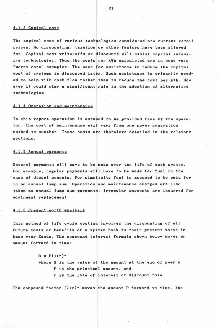
4 .1 .6 Present worth analysis
This method of life cycle costing involves the discounting of all
future costs or benefits of a system back to their present worth in
base year Rands. The compound interest formula shown below moves an
amount forward in time:
S = P(l+r)n
where S is the value of the amount at the end of year n
P is the principal amount, and
r is the rate of interest or discount rate .
The compound factor (1+r)n moves the amo~nt P forward in time , the
22
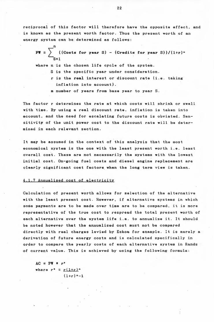
reciprocal of this factor will therefore have the opposite effect, and
is known as the present worth factor . Thus the present worth of an
energy system can be determined as follows :
n
PW = ~ ((Costs for yearS) - (Credits for year S))/(l+r)•
S=l
where n is the chosen life cycle of the system.
S is the specific year under consideration .
r is the real interest or discount rate (i . e . taking
inflation into account).
m number of years from base year to year S.
The factor r determines the rate at which costs will shrink or swell
with time. By using a real discount rate, inflation is taken into
account, and the need for escalating future costs i s obviated . Sen
sitivity of the unit power cost to the discount rate will be de ter
mined in each relevant section.
It may be assumed in the context of this analysis that the most
economical system is the one with the least present worth i.e . least
overall cost. These are not necessarily the systems with the lowest
initial cost. On-going fuel costs and diesel engine replacement are
ciearly significant cost factors when the long term view is taken.
4.1.7 Annualised cost of electricity
Calculation of present worth allows for selection of the alternative
with the least present cost . However, if alternative systems in wh ic h
some payments are to be made over time are to be compared , it is more
representative of the true cost to respread the total present worth of
each alternative over the system life i.e. to annualise it. It should
be noted however that the annualised cost must not be compared
directly with real charges levied by Eskom for example . It is merely a
derivation of future energy costs and is calculated specifically in
order to compare the yearly costs of each alternative system in Rands
of current value. This is achieved by using the following formula:
AC : PW * r•
where r• = r(l+r)n
(l+r)n-1

23
This annualised cost can be further interpreted by dividing it by the
::~;c:::l:::u:~.":::u~c:::~;~ ::i:":::·n::r:h:•::hm~::.::,::k•;o:o example, because of oversizing, iesel plant may generate significant
unused power in low load periods and this should not be given credit
in the analysis.
4.2 CONCLUSION
The aforementioned methodology will be applied to the various avail
able systems for remote area power supply. Where necessary, further
parameters will be specified in he relevant sections. In addition,
sensitivity of the unit power cost for the various alternatives to
relevant parameters will be giveA in relevant sections.
24
CHAPTER FIVE
CURRENT DIESEL POWER GENERATING PRACTICES AND COSTS
Electricity used in remote areas of South Africa was for many year s
provided by a variety of rudiment•ry systems. Storage batteries played
a large part in these installations, which were usually low voltage
12, 24 or 32V DC. Small diesel or petrol generators, often supple
mented by small wind chargers were used to charge the batteries. Power
use was limited to lights and the few DC appliances that may have been
available.
The late 1940s and 1950s saw the advent of reliable diesel generators
and relatively low fuel costs, while at the same time the demand for
220V AC supply was growing. With these generators, the owner was ab l e
to purchase and run normal appliances and, most importantly , to r un
refrigeration equipment. As a result the wind driven plant. and 32V
battery banks rapidly faded into insignificance, and today can on ly be
found in use in very few places, usually providing lighting powe r
only.
Until the 1970s, the diesel generator appeared to be the satisfactory
solution for remote area power supply . However, fuel cost and avail
ability, and mounting service costs are placing operators of such
plant under increasing pressure. Most installations are now operated
on a restricted time basis, typically 5- 10 hours per day . Ev en with
these restrictions many installations are grossly unde r ut il ised ,
wasting up to 80% of the fuel used, through poor load matching. Main
tenance costs are also increased as a result of this, and complete
engine overhaul or replacement · is often required after only 3500
5500 hours operation.
In the period discussed above, there were also a significant number of
towns and villages which were dependent on diesel - for their electr i
city supply. Gradually, as the electrification of the railways took
Eskom further out into the rural areas , so the numbe r o f t hese la r ge
gensets decreased. The petroleum price increases of the 19 70s was the
next stimulus for the extension of the national grid . There are now no
settlements of substantial proportions dependent on large scale diesel
power generation. ·
25
5 . 1 REMOTE AREA POWER SUPPLY REQ IREMENTS
The necessary or desired (as opposed to currently achieved) electric
ity requirements for domestic and commercial agricultural power supply
may be summarised by specifying the two basic parameters; load profile
and power supply quality.
5. 1 .1 Load profile
Th i s basically consists of a curve of instantaneous power demand
plotted against the time of day, but includes peak load, power avail
ab i lity, average load, and the load factor relationship (ratio of
average power to peak demand). As an historical feature this curve can
be used to analyse patterns of usage. Unfortunately little work has
been done on typical load profiles for consumers in remote areas
either in South Africa or internationally . If an alternative power
source is to be considered by a consumer, current demand patterns need
to be analysed. In the case of grid power being supplied, this analy
sis needs to be extrapolated to take into account the changes that
take place when conventional power supply is made available.
Currently, where power is supplied by diesel generator alone, the
measured load profile could be confused by false load added to the
system to ensure adequate or optimum engine loading. An additional
confusion occurs because the consumer may have an atypical lifestyle,
based on activities centred around times when the diesel generator is
running, e.g . such activities as washing and ironing are crammed into
evening periods. It is obvious that these patterns may differ from
household to household, thus nee ssitating a very comprehensive survey
of load patterns and the factors affecting them.
In considering the required power supply rather than the historical
pa t terns, it is not practical to speculate on the shape of the load
profile . It is , however possible to discuss the main features to be
expected. These include the peak (or maximum) load, hours per day
power is made available, average load, load and capcity factor.
Peak load is reached when a significant number of appliances are
turned on together, and is particularly noticeable if motor starting
loads are included. Peak load, measured in kW, is the largest sum of

26
expected appliance loads operating at any one time. With the main
domestic loads being say, a refrigerator, air conditioner, freeze r,
coolroom, washing machine and other normal household appliances , plus
some workshop tools, a peak load of 10 kW might be expected . Clearly
this will vary somewhat from one consumer to another, depending on
other loads which may be supplied from the same source , e . g . welding
or shearing equipment. It has been ~ound through discussion with
various equipment suppliers , consumers and engineers of the Department
of Agricultural Engineering that at as a general rule 10 kW peak
system capacity is required by most farmers. How often this is
achieved in practice is the subject of a later section.
Peak load requirements are high if refrigeration, coolroom and air
conditioning loads are in use. As the main advantage of conventional
power is its 24-hour availability, thus making cooling load possible
where currently it may not be, the peak load requirements are not
likely to fall with changing supply conditions.
For effective cooling load, power is required 24 hours per day , unless
specially designed heavy insulation freezers are used . Currently dura
tions of 10-16 hours/day are common . Continuous supply is however the
ideal for ~11 consumers . This makes the use of electric cooling poss
ible, eases lifestyle by reduc i ng the degree to which activities using
power have to be managed, and allows for the use of a wider range of
useful appliances.
Difficulty with the timetabling of activities to coincide with diesel
genset operating t i mes i s a constant frustration . Co nverse l y a g r eat
deal of fuel is wasted by the mismatch of act i v i ties and d i esel
running times. Thus 24-hour availability is a requirement if reason
able alternate electricity supply is to be contemplated . Lack of a
constant power supply has resulted in a variety of alternative power
sources being used - LPG, wood , direct diesel engine power etc.
Current quantities of power generated vary widely depending upon the
methods and modes of generation used by individuals.
Consumptions varying as widely as from 5 to 48 kWh/day were noted i n
the farm quest i onnaire replies, with 8 to 10 kWh/ day be i ng the most
common.

27
An installation that has a very high peak demand but a low average
demand will require a different generation system to an installation
with a more closely matched peak and average demand. The relationship
between peak and average demand (averaged over a 24-hour period),
expressed as a ratio is termed the· load factor. This ratio is usually
expressed as the average divided by the peak. Thus the homestead with
a peak demand of 10 kW and an average demand of 417 W would have a
load factor of 0,04 . By way of comparison the load factors for Lady
Frere and Cala in the Transkei were 0,69 and 0,46 respectively, in
1979 (Hill Kaplan Scott and Partners, 1979). Both these towns had
diesel generator systems at the time, but with fairly well distributed
loads. These larger, more sustained loads are provided by consumers
such as hospitals and small industries .
In the case of smaller installations, the addition of battery storage
and the use of correct charge characteristics results in a load factor
dur i ng charging, of typically 0,95 (recovery rate) to 0,68 (finished
rate). More will be said about such systems in the section dealing
with hybrid installations.
Another parameter to be considered here is capacity factor. The capa
city factor of a system is defined as the ratio of the nett amount of
power delivered by the system to that potentially able to be supplied,
dur i ng the period for which it is running. Thus an installation that
runs a diesel generator set at high load, for a few hours each day,
may have a low load factor but a high capacity factor , which would
result in optima1 diesel use. However, if the generator running time
were extended to give a 24-hour supply, it would be underutilised, and
thus have a low capacity factor as well.
Of t en a high capacity factor is achieved by adding unnecessary load,
sometimes known as a "load dump". This is not to be confused with load
shedding, which is in fact the exact opposite. Load dumping is often
of no financial benefit to the operator of the generator set, thus
when calculating a capacity factor all such loads should generally be
ignored. A sensible method of load dumping is to use the excess power
for water heating.
A comparison of the load and capacity factors gives an indication of
whe t her some form of storage would be of benefit to the overall
operating efficiency of the system. If, for example, the capacity and
28
load factors are both above 0,8 then nothing would be gained by the
addition of some storage system. If, however, the capacity factor is
below 0,5, there could well be a case for some storage medium. It is
general sound practice for diesel engine protection and optimum
performance to ensure that the capacity factor is better than 0,8 .
Contrary to popular belief, fuel savings are not achieved by low
loading of a diesel engine. Peak fuel efficiency occurs close to peak
engine performance, and · low loading could lead to engine damage .
Finally, power factor is a measure of the power actually available for
use from a generating source. By virtue of the fact that the voltage
and current may be out of phase, the full power kilowatts delivered
will be lower than the kVA rating of the generator .
5.1.2 Power supplY quality
This concept embraces voltage fluctuations, frequency stability, and
the waveform of a particular system. In general 220V AC , 50Hz e l ect ri
city supply is required in rural areas, with 380V AC. three-phase
being required where heavier machinery is to be used. To give some
indication, the all-electric urban home, annual consumption typical l y
exceeds 5 000 kWh, with a peak capacity of 5 kVA. voltage regulation
of ±6% and frequency stability of ±5% .
Modern diesel gensets can usually maintain an accurate sinusoidal
waveform . However, many alternative sources generate some other wave
form. In the case of most inverters it is a modified square wave . Pure
square waves may cause motor heating problems as well as producing
unacceptable levels of radio frequency interference .
5.2 CURRENT GENERATING PRACTICES
Current practice for generating power in remote off-grid areas of the
country can only be described as the sum of many individuals' attempts
to meet their needs for electrical power . Systems range from 32V DC
wind-powered generators with ancient single-cylinder slow-running
Lister engine backup, through .to modern 25 kVA, and larger , turbo
charged diesel gensets which run for 16 hours or more per day . Ma i n
tenance is also just as varied, and generally sub-standard.
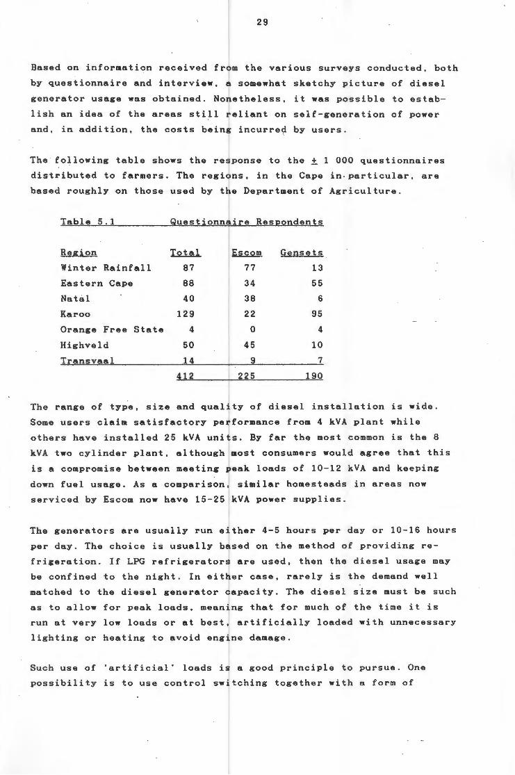
29
Based on information received from the various surveys conducted, both
by questionnaire and interview, ~ somewhat sketchy picture of diesel
generator usage was obtained. Nonetheless, it was possible to estab
lish an idea of the areas still reliant on self-generation of power
and, in addition, the costs being incurre~ by users.
The following table shows the response to the ± 1 000 questionnaires
distributed to farmers. The regions, in the Cape in - particular, are
based roughly on those used by the Department of Agriculture.
Table 5.1 Questionnaire Respondents
Region Total Escom Gensets
Winter Rainfall 87 I 77 13
Eastern Cape 88 34 55
Natal 40 38 6
Karoo 129 22 95
Orange Free State 4 0 4
Highveld 50 45 10
Transvaal 14 9 7
412 225 190
The range of type, size and quality of diesel installation is wide.
Some users claim satisfactory performance from 4 kVA plant while
others have installed 25 kVA units. By far the most common is the 8
kVA two cylinder plant, although most consumers would agree that this
is a compromise between meeting peak loads of 10-12 kVA and keeping
down fuel usage. As a comparison, similar homesteads in areas now
serviced by Escom now have 15-25 ,kVA power supplies .
The generators are usually run either 4-5 hours per day or 10-16 hours I
per day. The choice is usually based on the method of providing re-
frigeration . If LPG refrigerators are used, then the diesel usage may
be confined to the night. In either case, rarely is the demand well
matched to the diesel generator capacity. The diesel size must be such
as to allow for peak loads, meaning that for much of the time it is
run at very low loads or at best, artificially loaded with unnecessary
lighting or heating to avoid engine damage .
Such use of 'artificial' loads is a good principle to pursue. One
possibility is to use control switching together with a form of
30
storage, such as a water heating load. This would be switched on and
off as other loads varied, and would mean that a better match of
genset output to load is achieved, thus reducing chances of engine
damage. This practice is on the increase in Australia, however it is
doubted whether such management is practised at all in South Africa .
Certainly no mention of it was made by any respondents to the
questionnaire.
Short duration diesel systems do not usually provide refrigeration
load and would typically be run at night to provide lighting and some
. appliance loads, typically a washing machine and TV. The average load
over 24 hours for such systems may be 400-SOOW, however their load
profile for the running time usually shows a continuous high load for
the set (2-4 kW). This applies especially when the consumers are well
organised and undertake those tasks requiring electricity in the few
hours of operating time. If the diesel set is small (4-6 kVA), then
the capacity factor may be as high as 0,75. If it is of larger capa
city or if the consumers are not well-organised, the capacity factor
may be as low as 0,03. This means that not only is the diesel engine
wasting fuel but it may also suffer from underloading resulting in
carbonation, cylinder glazing and shorter life.
In systems where the diesel set is used for semi-permanent power
supply including refrigeration load, the average load might ' be 500-
700W. The load profile in this case may again show a high peak and low
capacity factor with the same engine damage as a resuit. It is usual
in these installations to have some dummy load connected to ensure
adequate engine loading at all times . This false load leads to unne
cessary fuel usage and poor economics but does preserve the engine .
The justification for longer run times is either to give refrigeration
plant time . to maintain coolth and/or to provide convenient power
supply. Whatever the reason the practice usually results in very low
load and capacity factors, meaning the system is quite unsatisfactory.
5.3 DIESEL GENERATING COSTS
Considering that there are about as many operating modes of diesel
gensets as there are gensets themselves, it would be impossible to
determine a typical load profile for a self generation power supply .
Thus in order to determine the real costs to the consumer of diesel I

31
power generation, two approaches r ere taken. Firstly, a simple micro
computer based diesel genset model was developed, and secondly field
monitoring of a limited number of diesel genset systems was carried
out to determine real operating fuel and power consumption.
5.3 . 1 Simulation of Diesel Genset Operation
A micro-computer based mathematical model was developed to simulate
the running of a diesel genset under various conditions. The model was
written in BASIC, and a listing of it can be found in Appendix C.
Briefly, the model allows the user to input a particular load curve
and to stipulate the degree to which the genset can be oversized for
the application e.g. 50%. The gensets capable of meeting the load
requirements are then selected frpm a database. The selected gensets
are then 'run' against the synthesised load curve to determine the
fuel consumption for the given cycle .
These consumption figures are then fed into a life cycle costing
routine set up in a spreadsheet, and the cost of running the genset
over a time period is then determined, taking into account all capital
and running costs.
Load Curves
As said earlier, with the variety of different genset installations
there is as wide a range of load profiles. For this reason load curves
for various typical applications were synthesised, based on the typi
cal power consumptions for various household appliances, workshop
equipment and agricultural machinery e.g. milking machines, pumps,
welding equipment etc.
Diesel Engine Fuel Consumptions
This is a further area of uncertainty, as the consumption figures
usually given by manufacturers are for an engine at full load. If an
engine is run at less than this load, there is a fuel saving in pro
portion to the reduction in load. This is however only true up to a
point beyond which the engine will use fuel regardless of the load.
For example this occurs at 30% load on at least one popular make of
engine. Peak engine performance and long engine life is achieved when
the unit is run near full load, or full fuel flow.
32
Diesel consumption data was supplied by manufacturers, either in the
form of engine maps, or consumption tables based on British. SAE or
DIN standard tests. From these data mathematical correlations for
specific fuel consumption vs percentage of full load were determined.
A factor was Quilt into the model to enable the derating of the engine
due to altitude to be taken into account . Rated capacity is reduced by
±4% for each 300m increase in elevation above sea-level (Calloway,
1985).
5.3.2 Determination of Diesel Generation Costs
The diesel consumption results obtained from the mathematical model
were used to calculate the unit power costs of diesel power genera
tion. This was done by first calculating the present worth of the
power plant, its operation and maintenance over a fixed period. A
levelized annual cost was determined from this value, and then divided
by the power consumed per year to obtain the cost per kilowatthour .
For these calculations, assumptions had to be made regarding certain
parameters. Careful note should be taken of these assumptions when
comparing these costs with those incurred using other forms of remote
area power supply.
Before undertaking the detailed cost analysis, the effects of some of
these parameters are examined by means of parametric sensitivity ana
lyses on data obtained from simulation of a diesel genset used to
supply power for domestic use. The maximum demand of this base case
system is 4,0 kVA with a daily consumption of 14 , 75 kWh , consumed over
a period of 5,75 hours. The replacement engine age is taken as 15 000
hours, the real discount rate as 5% and the price of diesel as 55c/l.
The diesel price chosen falls in the middle of the price range paid by
farmers for agricultural diesel. There is a wide variation of prices,
dependent on location and whether a particular farmer is eligible for
.rebates from the Department of Customs and Excise. 55 c/1 is therefore
chosen as the price to be used in all the analyses in this report.
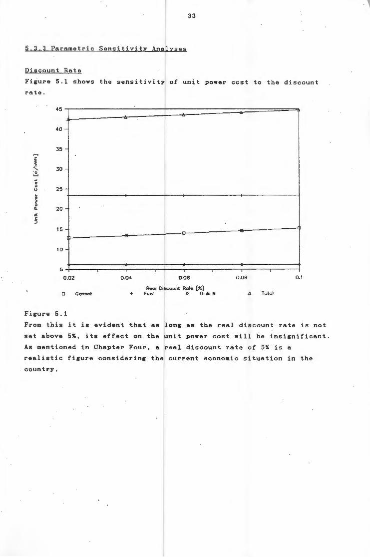
33
5.3 . 3 Parametric Sensitivity Analyses
Discount Rate
Figure 5.1 shows the sensitivity of unit power cost to the discount
rate.
45
40 -
35 -,..... ~
~ ~
' 30 ·u -...... .. " 0
25 u -1.. D ~ 0 ll. 20 -::! c ;)
15 - -
10 -
5 I I
0 .02 0 .04 0.06 0.08 0 .1
Real Discount Rote [%] 0 Genset + Fuel 0 0 &c Ill Total
Figure 5.1
From this it is evident that as long as the real discount rate is not
set above 5%, its effect on the unit power cost will be insignificant.
As mentioned in Chapter Four, a real discount rate of 5% is a
realistic figure considering the current economic situation in the
country .
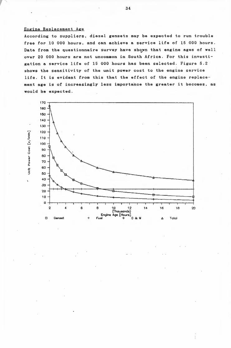
34
Engine Replacement Age
According to suppliers, diesel gensets may be expected to run trouble
free for 10 000 hours, and can achieve a service life of 15 000 hours .
Data from the questionnaire survey have sh~wn that engine ages of wel l
over 20 000 hours are not uncommon in South Africa . For this investi
gation a service life of 15 000 hours has been selected . Figure 5 . 2
shows the sensitivity of the unit power cost to the engine service
life . It is evident from this that the effect of the engine replace
ment age is of increasingly less importance the greater it becomes, as
would be expected.
170
160
150
140
130 ,..., 120 .s:: ~
110 .X
"-u 100 ...... .. ., 90 0
u ... 80 Cl ~ 70 0
Q.
:!. 60 c ::> so
40
30
20
10
0
c
2 4 6
Gen:set +
8 10 12 14 (Tt-.ousands}
Enr;ine Aqe (Hout"2] Fuel 0 0 & 1.1
16 18 20
4 Totol
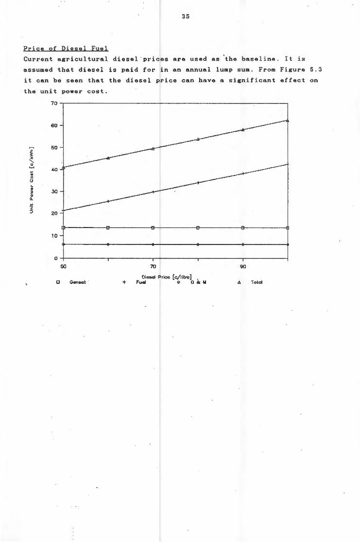
35
Pr i ce of Diesel Fuel
Current agricultural diesel · prices are used as 'the baseline. It is
assumed that diesel is paid for in an annual lump sum. From Figure 5 . 3
it can be seen that the diesel price can have a significant effect on
the unit power cost.
60
,.-, 50 .r. ~
"' -...... u ....... 40 .. " 0 0 ... D
30 ~ 0 n. = I: ::> 20
10
0 ~----------~------------r-----------~----------~----------~ 50 70 90
Diesel Price [c/litre) • 0 Genset · + Fuel o 0 & lol Totol
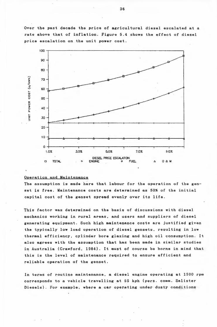
36
Over the past decade the price of agricultural diesel escalated at a
rate above that of inflation. Figure 5.4 shows the effect of diesel
price escalation on the unit power cost.
100
90
80
'"' &. 70 ~ .>t.
-;,. '-" 60 .... U)
0 0 50 II: 11.1 ~ 40 0 n. !:: z 30 :J
20
10
0
1.0% 3.0% 5.0% 7.0% 9.0%
DIESEl. PRICE ESCALATION 0 TOTAL + ENGINE ~ FUEl. ll.. 0 & 1.4
Operation and Maintenance
The assumption is made here that labour for the operation of the gen
set is free. Maintenance costs are determined as 50% of the initial
capital cost of the genset spread evenly over its life .
This factor was determined on the basis of discussions with diesel
mechanics working in rural areas, and users and suppliers of diesel
generating equipment. Such high maintenance costs are justified given
the typically low load operation of diesel gensets, resulting in low
thermal efficiency, cylinder bore glazing and high oil consumption. It
also agrees with· the assumption that has been made in similar studies
in Australia (Crawford, 1984). It must of course be borne in mind that
this is the level of maintenance required to ensure efficient and
reliable operation of the genset.
In terms of routine maintenance, a diesel engine operating at 1500 rpm
corresponds to a vehicle travelling at 55 kph (pers. comm. Salister
Diesels) . For example, where a car operating under dusty conditions
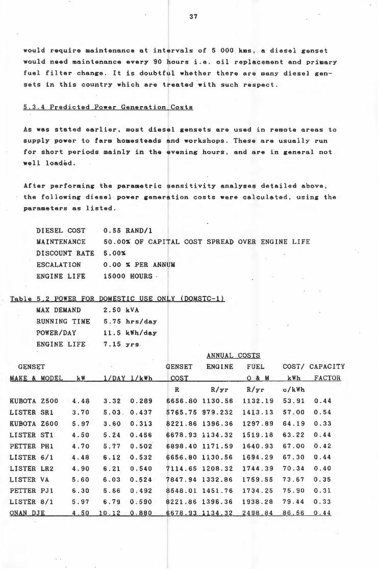
37
would require maintenance at intervals of 5 000 kms, a diesel genset
would need maintenance every 90 hours i.e. oil replacement and primary
fuel filter change. It is doubtful whether there are many diesel gen
sets in this country which are treated with such respect.
5 .3 .4 Predicted Power Generation Costs
As was stated earlier, most diesel gensets are used in remote areas to
supply power to farm homesteads and workshops. These are usually run
for short periods mainly in the evening hours, and are in general not
well loaded.
After performing the parametric sensitivity analyses detailed above,
the following diesel power generation costs were calculated, using the
parameters as listed.
Table
DIESEL COST
MAINTENANCE
DISCOUNT RATE
ESCALATION
ENGINE LIFE
5.2 POWER FOR
MAX DEMAND
RUNNING TIME
POWER/DAY
ENGINE LIFE
GENSET
MAKE &. MODEL kW
KUBOTA zsoo 4.48
LISTER SR1 3.70
KUBOTA Z600 5.97
LISTER ST1 4.50
PETTER PH1 4 . 70
LISTER 6/1 4.48
LISTER LR2 4.90
LISTER VA 5.60
PETTER PJl 6.30
LISTER 8/1 5.97
ONAN DJE 4.50
0.55 RAND/1
SO.OOS OF CAP! AL COST SPREAD OVER ENGINE LIFE
5.00%
0.00 % PER ANNUM
15000 HOURS ·
DOMESTIC USE ONLY
2.50 kVA
5.75 hrs/day
11.5 kWh/day
7.15 yrs .
{DOMSTC-1)
GENSET
COST
ANNUAL COSTS
ENGINE FUEL COST/ CAPACITY
1/DAY l/kWh 0 & M kWh FACTOR
R R/yr R/yr c/kWh
3.32 0.289 6656.80 1130. 56 1132.19 53.91 0 . 44
5.03 . 0.437 5765.75 979.232 1413.13 57.00 0.54
3.60 0.313 8221.86 1396.36 1297.89 64.19 0.33
5.24 0.456 6678.93 1134.32 1519 . 18 63.22 0.44
5 . 77 0 . 502 6898.40 1171.59 1640.93 67.00 0 . 42
6.12 0.532 6656.80 1130.56 1694.29 67.30 0.44
6.21 0 . 540 7114.65 1208.32 1744 . 39 70.34 0 . 40
6.03 0.524 7847.94 1332.86 1759.55 73.67 0.35
5.66 0.492 8548.01 1451 . 76 1734.25 75.90 0.31
6.79 0.590 8221.86 1396.36 1938.28 79.44 0.33
10.12 0.880 6678.93 1134.32 2498.84 86 . 56 0.44
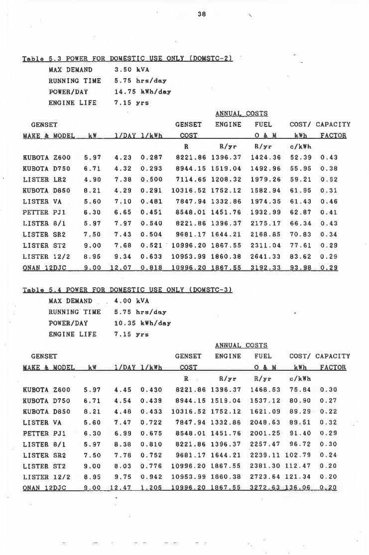
38
Table 5.3 POWER FOR DOMESTIC USE ONLY {DOMSTC-2}
MAX DEMAND 3.50 kVA
RUNNING TIME 5.75 hrs/day
POWER/DAY 14.75 kWh/day
ENGINE LIFE 7.15 yrs
ANNUAL COSTS
GENSET GENSET ENGINE FUEL COST/ CAPACITY
MAKE &:. MODEL kW lLDAY lLkWh COST 0 & M kWh FACTOR
R R/yr R/yr c/kWh
KUBOTA Z600 5.97 4.23 0.287 8221.86 1396.37 1424 . 36 52 . 39 0.43
KUBOTA D750 6.71 4.32 0.293 8944.15 1519.04 1492.96 55.95 0 . 38
LISTER LR2 4.90 7.38 0.500 7114.65 1208.32 1979.26 59 . 21 0.52
KUBOTA D850 8.21 4.29 0.291 10316.52 1752.12 1582.94 61.95 0.31
LISTER VA 5.60 7.10 0.481 7847.94 1332.86 1974.35 61.43 0.46
PETTER PJ1 6.30 6.65 0.451 8548.01 1451.76 1932.99 62.87 0.41
LISTER 8/1 5.97 7.97 0.540 8221 . 86 1396 . 37 2175.17 66.34 0 . 43
LISTER SR2 7 . 50 7.43 0.504 9681.17 1644 . 21 2168 . 85 70 . 83 0 . 34
LISTER ST2 9.00 7.68 0.521 10996.20 1867.55 2311.04 77 . 61 0 . 29
LISTER 12/2 8.95 9.34 0.633 10953.99 1860 . 38 2641 . 33 83.62 0.29
ONAN 12DJC 9.00 12.07 0.818 10996.20 1867.55 3192 . 33 93.98 0 . 29
Table 5.4 POWER FOR DOMESTIC USE ONLY {DOMSTC-3}
MAX DEMAND 4.00 kVA
RUNNING TIME 5 . 75 hrs/day
POWER/DAY 10.35 kWh/day
ENGINE LIFE 7.15 yrs
ANNUAL COSTS
GENSET GENSET ENGINE FUEL COST/ CAPACITY
MAKE & MODEL kW lLDAY lLkWh COST 0 & M kWh FACTOR
R R/yr R/yr c/kWh
KUBOTA Z600 5.97 4.45 0.430 8221.86 1396 . 37 1468 . 53 75 . 84 0.30
KUBOTA D750 6.71 4.54 0.439 8944.15 1519 . 04 1537.12 80.90 0.2 7
KUBOTA D850 8.21 4.48 0.433 10316.52 1752.12 1621.09 89.29 0 . 22
LISTER VA 5.60 7.47 0.722 7847.94 1332.86 2048.63 89.51 0 . 32
PETTER PJ1 6.30 6.99 0.675 8548.01 1451 . 76 2001 . 25 91 . 40 0 . 29
LISTER 8/1 5.97 8.38 0.810 8221 . 86 1396 . 37 2257.47 96 . 72 0 . 30
LISTER SR2 7.50 7.78 0.752 9681. 17 1644 . 21 2239 .1 1 102 .7 9 0 . 24
LISTER ST2 9.00 8.03 0.776 10996 . 20 1867 . 55 2381.30 112 . 47 0 . 20
LISTER 12/2 8.95 9.75 0 . 942 10953.99 1860.38 2723 . 64 121 . 34 0 . 20
ONAN 12DJC 9.00 12.47 1.205 10996.20 1867 . 55 3272.63 136 . 06 0 . 20
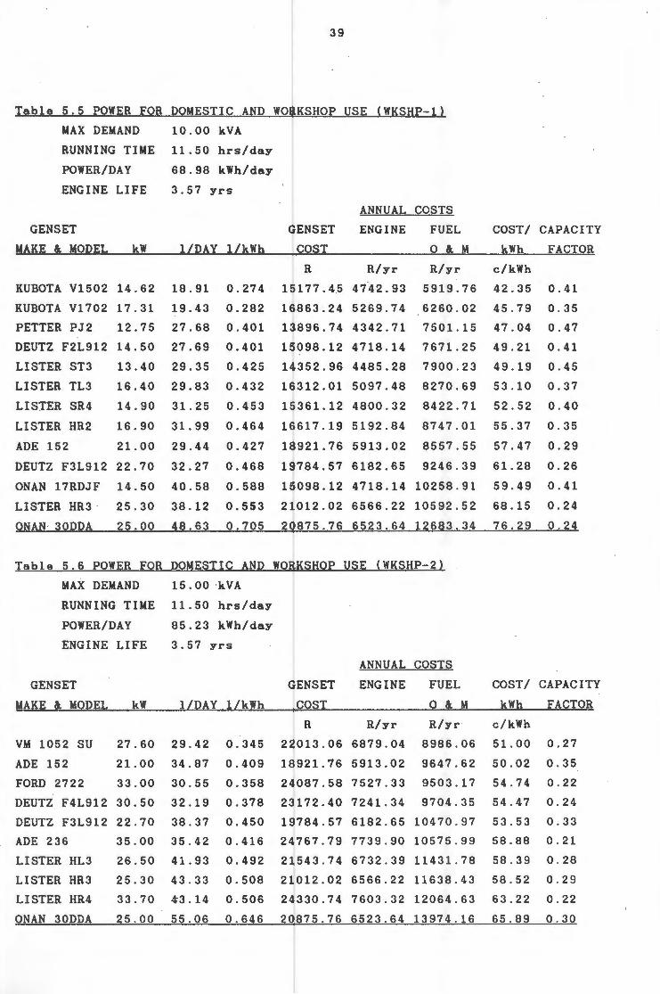
39
Table 5.g POWER FOR DOMESTIC AND WORKSHOP USE (WKSHP-1}
MAX DEMAND 10 . 00 kVA
RUNNING TIME 11 . 50 hrs/day
POWER/DAY 68 . 98 kWh/day
ENGINE LIFE 3 . 57 yrs
ANNUAL COSTS
GENSET GENSET ENGINE FUEL COST/ CAPACITY
MAKE &. MODEL kW l[DAY l[kWh COST 0 &. M kWh FACTOR
R R/yr R/yr c/kWh
KUBOTA V1502 14 . 62 18.91 0.274 15177.4.5 47-42.93 5919 . 76 42 . 35 0.41
KUBOTA V1702 17.31 19.43 0.282 16863.24 5269 . 74 6260.02 45 . 79 0.35
PETTER PJ2 . 12.75 27.68 0.401 13896.74 4342 . 71 7501 . 15 47 . 04 0.47
DEUTZ F2L912 14.50 27.69 0.401 15098.12 4718.14 7671 . 25 49.21 0.41
LISTER ST3 13.40 29.35 0.425 14352.96 4485.28 7900 . 23 49.19 0.45
LISTER TL3 16.40 29.83 0 . 432 16312.01 5097 . 48 8270 . 69 53.10 0.37
LISTER SR4 14.90 31.25 0.453 15361.12 4800 . 32 8422 . 71 52 . 52 0 . 40
LISTER HR2 16 . 90 31 . 99 0.464 16617.19 5192.84 8747.01 55.37 0 . 35
ADE 1 52 21.00 29 . 44 0.427 18921.76 5913.02 8557 . 55 57.47 0 . 29
DEUTZ F3L912 22.70 32.27 0 . 468 19784.57 6182.65 9246 . 39 61 . 28 0.26
ONAN 17RDJF 14.50 40 . 58 0 . 588 15098.12 4718 . 14 10258 . 91 59 . 49 0.41
LISTER HR3 · 25 . 30 38.12 0.553 21012.02 6566.22 10592.52 68 . 15 0.24
ONAN · 30DDA 25.00 48.63 0.705 20875 . 76 6523.64 12683.34 76 . 29 0.24
Table 5.6 POWER FOR DOMESTIC AND WORKSHOP USE (WKSHP-2}
MAX DEMAND 15 . 00 kVA
RUNNING TIME 11.50 hrs/day
POWER/DAY 85 . 23 kWh/day
ENGINE LIFE 3.57 yrs
ANNUAL COSTS
GENSET GENSET ENGINE FUEL COST/ CAPACITY
MAKE &. MODEL kW l[DAY l[kWh COST 0 &. M kWh FACTOR
R R/yr R/yr c/kWh
VM 10 52 SU 27 . 60 29 . 42 0.345 22013.06 6879 . 04 8986 . 06 51.00 0.27
ADE 152 21.00 34.87 0.409 18921.76 5913.02 9647.62 50.02 0 . 35
FORD 2722 33.00 30.55 0 . 358 24087.58 7527.33 9503 . 17 54.74 0 . 22
DEUTZ F4L912 30 . 50 32.19 0.378 23172.40 7241 . 34 9704.35 54.47 0 . 24
DEUTZ F3L912 22.70 38 . 37 0 . 450 19784 . 57 6182 . 65 10470 . 97 53.53 0 . 33
ADE 236 35 . 00 35 . 42 0.416 24767 . 79 7739.90 10575.99 58 . 88 0 . 21
LISTER HL3 26 . 50 41 . 93 0.492 21543 . 74 6732.39 11431.78 58 . 39 0 . 28
LISTER HR3 25.30 43 . 33 0.508 21012.02 6566.22 11638 . 43 58 . 52 0 . 29
LISTER HR4 33 . 70 ¢3 . 14 0.506 24330.74 7603 . 32 12064 . 63 63.22 0 . 22
ONAN 30DDA 25 . 00 55.06 0.646 20875 . 76 6523 . 64 13974 . 16 65.89 0 . 30
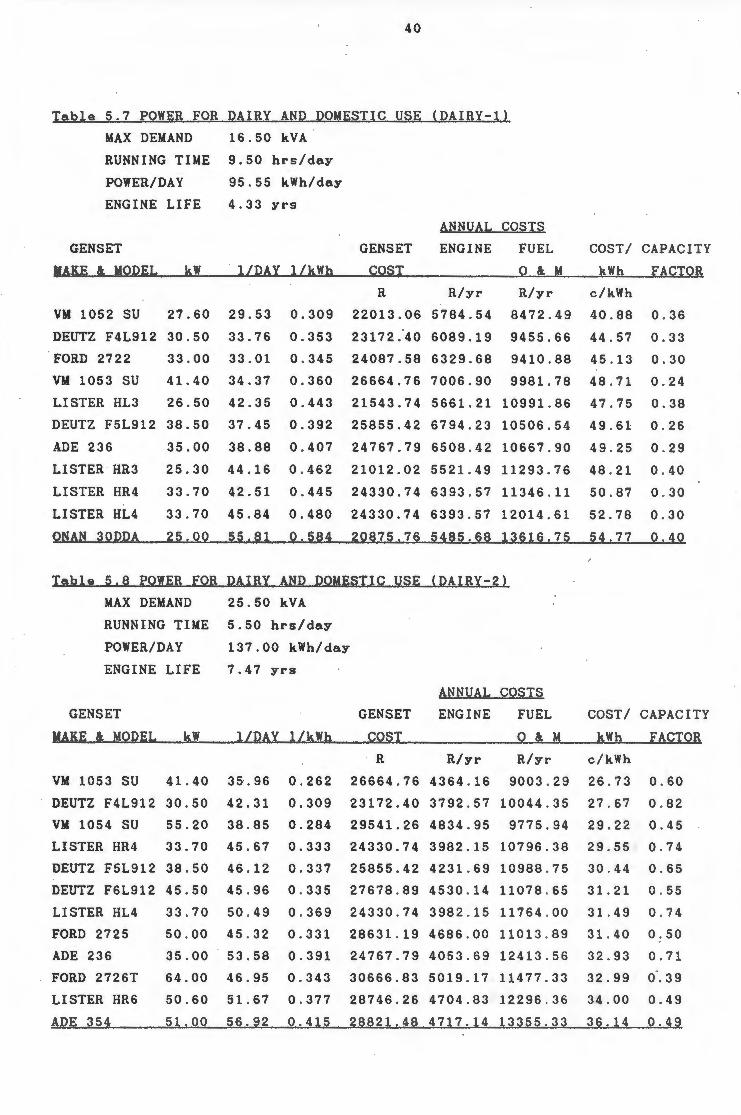
40
Table 5.7 POWER FOR DAIRY AND DOMESTIC USE (DAIRY-1}
MAX DEMAND 16.50 kVA
RUNNING TIME 9.50 hrs/day
POWER/DAY 95.55 kWh/day
ENGINE LIFE 4.33 yrs
ANNUAL COSTS
GENSET GENSET ENGINE FUEL COST/ CAPACITY
MAKE & MODEL kW lLDAY lLkWh COST 0 & M kWh FACTOR
R R/yr R/yr c/kWh
VM 1052 SU 27.60 29.53 0.309 22013.06 5784.54 8472.49 40.88 0 . 36
DEUTZ F4L912 30.50 33.76 0.353 23172.-40 6089.19 9455.66 44.57 0.33
FORD 2722 33.00 33.01 0.345 24087.58 6329.68 9410.88 45.13 0.30
VM 1053 SU 41.40 34.37 0.360 26664.76 7006.90 9981.78 48.71 0 . 24
LISTER HL3 26.50 42.35 0.443 21543.74 5661.21 10991.86 47.75 0.38
DEUTZ F5L912 38.50 37.45 0.392 25855.42 6794.23 10506.54 49.61 0.26
ADE 236 35.00 38.88 0 . 407 24767.79 6508.42 10667.90 49.25 0 . 29
LISTER HR3 25.30 44.16 0 . 462 21012.02 5521 . 49 11293.76 48 . 21 0 . 40
LISTER HR4 33.70 42.51 0 . 445 24330.74 6393 . 57 11346 . 11 50.87 0 . 30
LISTER HL4 33.70 45.84 0.480 24330.74 6393.57 12014.61 52.78 0.30
ONAN 30DDA 25.00 55.81 0.584 20875.76 5485.68 13616.75 54 . 77 0.40
Table 5.8 POWER FOR DAIRY AND DOMESTIC USE (DAIRY-2}
MAX DEMAND 25.50 kVA
RUNNING TIME 5.50 hrs/day
POWER/DAY 137.00 kWh/day
ENGINE LIFE 7.47 yrs
ANNUAL COSTS
GENSET GENSET ENGINE FUEL COST/ CAPACITY
MAKE & MODEL kW lLDAY lLkWh COST 0 & M kWh FACTOR
R R/yr R/yr c/kWh
VM 1053 SU 41.40 35·. 96 0.262 26664.76 4364 . 16 9003 . 29 26.73 0.60
DEUTZ F4L912 30.50 42.31 0.309 23172.40 3792 . 57 10044 . 35 27.67 0 . 82
VM 1054 SU 55.20 38.85 0.284 29541.26 4834.95 9775.94 29.22 0.45
LISTER HR4 33.70 45.67 0.333 24330.74 3982.15 10796.38 29.55 0.74
DEUTZ F5L912 38.50 46.12 0.337 25855.42 4231.69 10988.75 30.44 0.65
DEUTZ F6L912 45.50 45 . 96 0 . 335 27678.89 4530 . 14 11078 . 65 31.21 0 . 55
LISTER HL4 33 . 70 50 . 49 0 . 369 24330 . 74 3982 . 15 11764 . 00 31 . 49 0 . 74
FORD 2725 50.00 45 . 32 0.331 28631.19 4686 . 00 11013 . 89 31 . 40 0 . 50
ADE 236 35.00 53.58 0.391 24767.79 4053.69 12413 . 56 32 . 93 0.71
FORD 2726T 64.00 46.95 0.343 30666.83 5019.17 11477.33 32.99 o·. 39
LISTER HR6 50.60 51.67 0.377 28746.26 4704.83 12296 . 36 34.00 0.49
ADE 354 51.00 56.92 0.415 28821.48 4717.14 13355 . 33 36.14 0.49
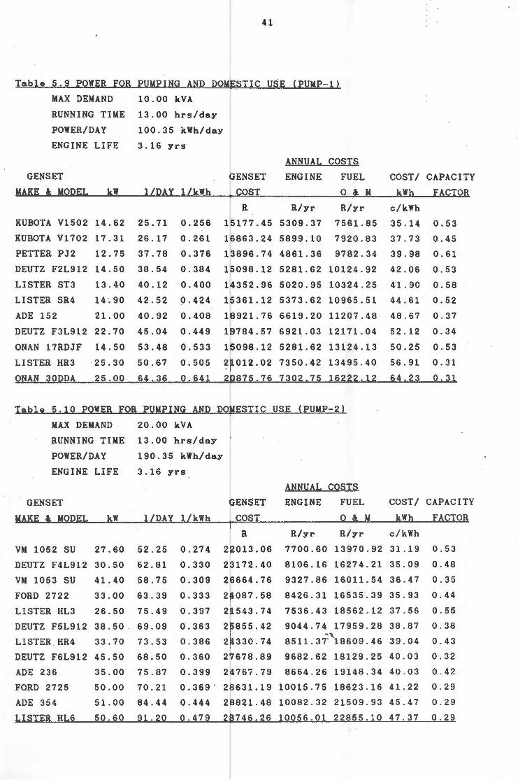
41
Table 5.9 POWER FOR PUMPING AND DOMESTIC USE { PUMP-1}
MAX DEMAND 10.00 kVA
RUNNING TIME 13.00 hrs/day
POWER/DAY 100.35 kWh/day
ENGINE LIFE 3.16 yrs
ANNUAL COSTS
GENSET GENSET ENGINE FUEL COST/ CAPACITY
MAKE &. MODEL kW lLDAY lLkWh COST 0 &. M kWh FACTOR
R R/yr R/yr c/kWh
KUBOTA V1502 14.62 25.71 0.256 15177.45 5309.37 7561.85 35.14 0.53
KUBOTA V1702 17.31 26.17 0.261 16863.24 5899.10 7920.83 37.73 0.45
PETTER PJ2 12.75 37.78 0.376 13896.74 4861.36 9782.34 39.98 0.61
DEUTZ F2L912 14.50 38.54 0.384 15098.12 5281.62 10124.92 42.06 0 . 53
LISTER ST3 13.40 40.12 0.400 14352.96 5020.95 10324.25 41.90 0.58
LISTER SR4 14 ". 90 42.52 0.424 15361.12 5373.62 10965.51 44.61 0.52
ADE 152 21.00 40.92 0.408 18921.76 6619.20 11207.48 48.67 0.37
DEUTZ F3L912 22.70 45.04 0.449 19784.57 6921.03 12171.04 52.12 0.34
ONAN 17RDJF 14.50 53.48 0.533 15098.12 5281.62 13124.13 50.25 0.53
LISTER HR3 25.30 50.67 0.505 21012.02 7350.42 13495.40 56.91 0.31
ONAN 30DDA 25.00 64.36 0.641 20875.76 7302.75 16222.12 64.23 0.31
Table 5.10 POWER FOR PUMPING AND DOMESTIC USE {PUMP-2}
MAX DEMAND 20.00 kVA
RUNNING TIME 13.00 hrs/day
POWER/DAY 190.35 kWh/day
ENGINE LIFE 3.16 yrs
ANNUAL COSTS
GENSET GENSET ENGINE FUEL COST/ CAPACITY
MAKE &. MODEL kW lLDAY lLkWh COST 0 &. M kWh FACTOR
R R/yr R/yr c/kWh
VM 1052 SU 27.60 52.25 0.274 22013.06 7700.60 13970.92 31.19 0.53
DEUTZ F4L912 30.50 62.81 0.330 23172.40 8106.16 16274.21 35.09 0.48
VM 1053 SU 41.40 58.75 0.309 26664.76 9327.86 16011.54 36.47 0.35
FORD 2722 33.00 63.39 0.333 24087.58 8426.31 16535.39 35.93 0.44
LISTER HL3 26.50 75.49 0.397 21543.74 7536.43 18562 . 12 37.56 0.55
DEUTZ F5L912 38.50 69.09 0.363 25855.42 9044.74 17959.28 38.87 0 . 38
LISTER . HR4 33.70 73.53 0 . 386 24330.74 ~ " 8511. 37' 18609 . 46 39.04 0.43
DEUTZ F6L912 45.50 68.50 0.360 27678.89 9682.62 18129.25 40.03 0.32
ADE 236 35.00 75.87 0.399 24767.79 8664.26 19148 . 34 40.03 0.42
FORD 2725 50.00 70.21 0. 369. 28631.19 10015.75 18623.16 41.22 0.29
ADE 354 51.00 84.44 0.444 28821.48 10082.32 21509 . 93 45.47 0.29
LISTER HL6 50.60 91.20 0.479 28746.26 10056.01 22855.10 47.37 0.29
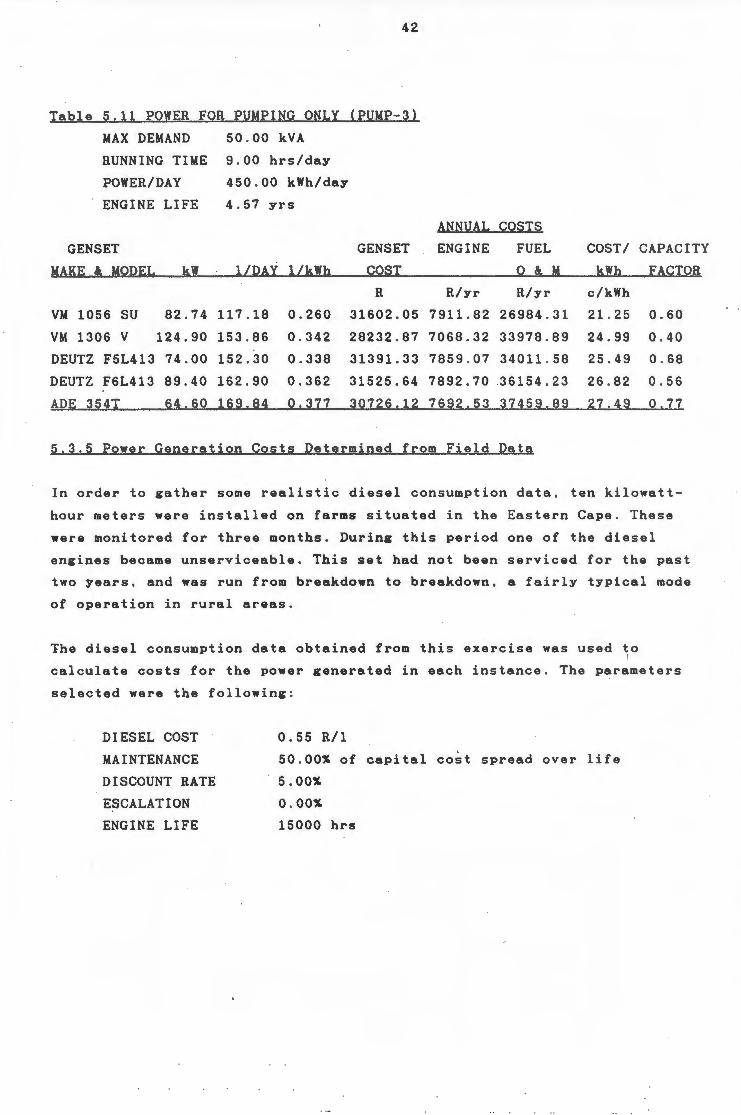
42
Table 5 . 11 POWER FOR PUMPING ONLY {PUMP-3}
MAX DEMAND 50 . 00 kVA
RUNNING TIME 9 . 00 hrs/day
POWER/DAY 450 . 00 kWh/day
ENGINE LIFE 4 . 57 yrs
ANNUAL COSTS
GENSET GENSET ENGINE FUEL COST/ CAPACITY
MAKE & MODEl, kW lLDAY lLkWh COST 0 &. M kWh FACTOR
R R/yr R/yr c/kWh
VM 1056 su 82.74 117.18 0.260 31602.05 7911.82 26984 . 3 1 21.25 0.60
VM 1306 v 124.90 153.86 0.342 28232.87 7068.32 33978 . 89 24 . 99 0 . 40
DEUTZ F5L413 74.00 152.30 0 . 338 31391.33 7859 . 07 34011 . 58 25.49 0 . 68
DEUTZ F6L413 89.40 162 . 90 0.362 31525 . 64 7892 . 70 .36154 . 23 26 . 82 0.56
ADE 354T 64 . 60 169.84 0.377 30726.12 7692.53 37459 . 89 27 . 49 0 . 77
5 . 3.5 Power Generation Costs Determined from Field Data
In order to gather some realistic diesel consumption data , ten kilowatt
hour meters were installed on farms situated in the Eastern Cape . These
were monitored for three months. During this period one of the diesel
engines became unserviceable. This set had not been serviced for the past
two years, and was run from breakdown to breakdown, a fairly typical mode
of operation in rural areas.
The diesel consumption data obtained from this exercise was used to
calculate costs for the power generated in each instance. The parameters
selected were the following :
DIESEL COST 0.55 R/1
MAINTENANCE 50 . 00% of capital cost spread over life
DISCOUNT RATE 5.00%
ESCALATION 0.00%
ENGINE LIFE 15000 hrs
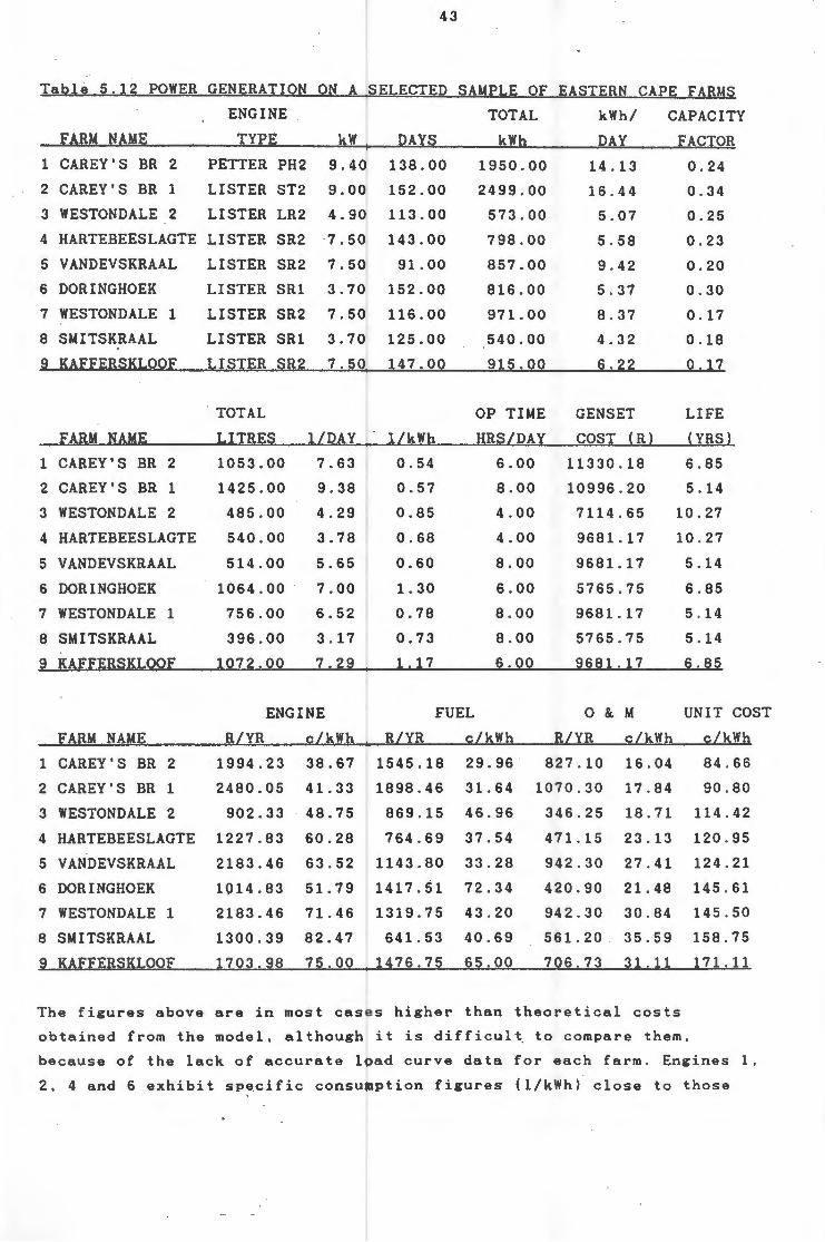
43
Table 5.12 POWER GENERATION ON A SELECTED SAMPLE OF EASTERN CAPE FARMS
ENGINE TOTAL kWh/ CAPACITY
FARM NAME TYPE kW DAYS
1 CAREY'S BR 2 PETTER PH2 9.40 138.00
2 CAREY'S BR 1 LISTER ST2 9 . 00 152.00
3 WESTONDALE 2 LISTER LR2 4.90 113 . 00
4 HARTEBEESLAGTE LISTER SR2 7.50 143.00
5 VANDEVSKRAAL
6 DORINGHOEK
7 WESTONDALE 1
8 SMITSKRAAL
9 KAFFERSKLOOF
FARM NAME
1 CAREY'S BR 2
2 CAREY'S BR 1
3 WESTONDALE 2
4 HARTEBEESLAGTE
5 VANDEVSKRAAL
6 DORINGHOEK
7 WESTONDALE 1
8 SMITSKRAAL
9 KAFFERSKLOOF
LISTER SR2
LISTER SR1
LISTER SR2
LISTER SR1
LISTER SR2
. TOTAL
LITRES
1053.00
1425.00
485.00
540.00
514.00
1064.00 .
756.00
396.00
1072.00
7.50
3.70
7.50
3.70
7.50
1/DAY
7.63
9.38
4.29
3.78
5.65
7.00
6.52
3 . 17
7.29
91.00
152.00
116.00
125.00
147.00
1/kWh
0.54
0.57
0.85
0.68
0.60
1. 30
0.78
0.73
1.17
kWh
1950.00
2499.00
573.00
798.00
857.00
816.00
971.00
540.00
915.00
OP TIME
HRS/DAY
6.00
8.00
4.00
4.00
8.00
6.00
8.00
8.00
6.00
DAY
14.13
16 . 44
5 . 07
5 . 58
9 . 42
5 . 37
8 . 37
4.32
6.22
GENSET
COST (R)
11330.18
10996 . 20
7114.65
9681.17
9681.17
5765.75
9681.17
5765.75
9681 . 17
ENGINE FUEL 0 & M
R/YR c/kWh FARM NAME R/YR c/kWh
1 CAREY'S BR 2 1994.23 38.67
2 CAREY'S BR 1 2480.05
3 WESTONDALE 2 902.33
4 HARTEBEESLAGTE 1227.83
5 VANDEVSKRAAL 2183.46
6 DORINGHOEK 1014.83
7 WESTONDALE 1 2183.46
8 SMITSKRAAL 1300.39
9 KAFFERSKLOOF 1703.98
41.33
48.75
60.28
63.52
51.79
71.46
82.47
75.00
R/YR c/kWh
1545.18 29.96
1898 . 46
869 . 15
764.69
1143.80
1417.51
1319.75
641.53
1476.75
31.64
46.96
37.54
33.28
72.34
43.20
40.69
65.00
827.10 16.04
1070 . 30
346 . 25
471.15
942.30
420.90
942.30
561.20
706.73
17 . 84
18.71
23.13
27.41
21.48
30.84
35 . 59
31 . 11
FACTOR
0 . 24
0.34
0.25
0.23
0.20
0.30
0.17
0.18
0.17
LIFE
(YRS)
6 . 85
5.14
10.27
10.27
5.14
6.85
5 . 14
5.14
6.85
UNIT COST
c/kWh
84.66
90.80
114.42
120.95
124.21
145 . 61
145 . 50
158 . 75
171.11
The figures above are in most cases higher than theoretical costs
obta i ned from the model , although it is difficult. to compare them.
because of the lack of accurate load curve data for each farm. Engines 1,
2, 4 and 6 exhibit specific consumption figures (1/kWh) close to those
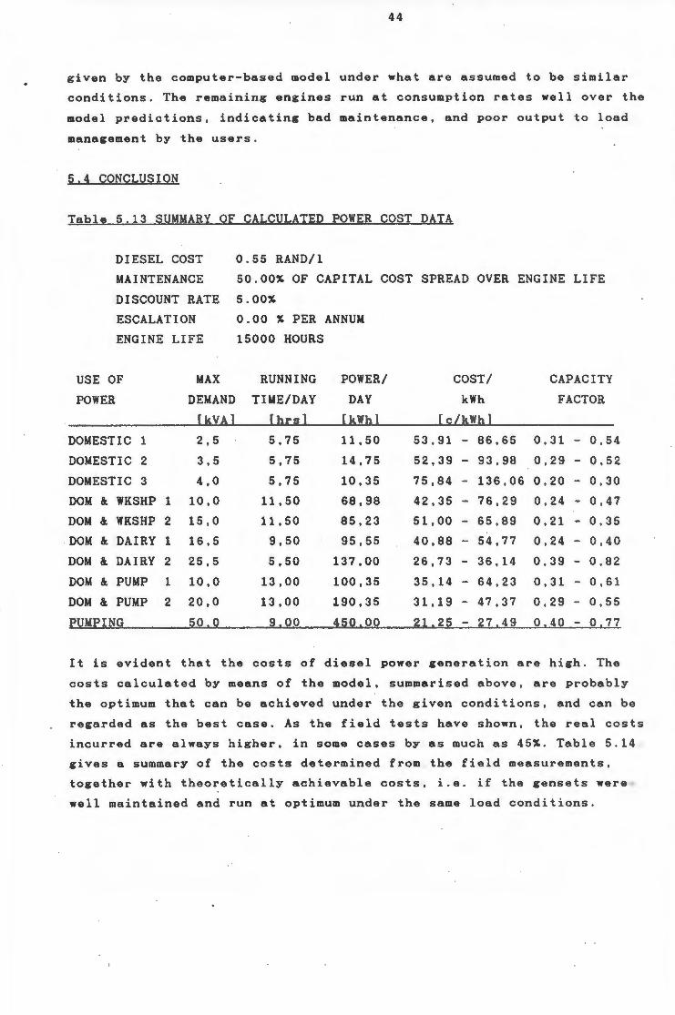
44
given by the computer-based model under what are assumed to be similar
conditions. The remaining engines run at consumption rates well over the
model predictions, indicating bad maintenance, and poor output to load
management by the users.
5.4 CONCLUSION
Table 5.13 SUMMARY OF CALCULATED POWER COST DATA
DIESEL COST 0.55 RAND/1
MAINTENANCE 50.00% OF CAPITAL COST SPREAD OVER ENGINE LIFE
DISCOUNT RATE 5.00%
ESCALATION 0.00 % PER ANNUM
ENGINE LIFE 15000 HOURS
USE OF MAX RUNNING POWER/ COST/ CAPACITY
POWER DEMAND TIME/DAY DAY kWh FACTOR
[kVA] [hrs] [kWh] [cLkWh]
DOMESTIC 1 2 , 5 5,75 11.50 53 , 91 - 86,65 0 , 31 - 0 , 54
DOMESTIC 2 3 , 5 5,75 14,75 52,39 - 93,98 0 , 29 - 0,52
DOMESTIC 3 4,0 5,75 10,35 75,84 - 136,06 0,20 - 0 , 30
DOM 8t WKSHP 1 10,0 11,50 68,98 42,35 - 76,29 0 , 24 - 0 , 47
DOM 8t WKSHP 2 15 , 0 11,50 85 , 23 51,00 - 65 , 89 0,21 - 0 , 35
DOM 8t DAIRY 1 16,5 9,50 95,55 40 , 88 - 54,77 0 , 24 - 0 , 40
DOM 8t DAIRY 2 25,5 5,50 137,00 26,73 - 36,14 0 , 39 - 0 , 82
DOM 8t PUMP 1 10,0 13,00 100,35 35,14 - 64,23 0,31 - 0,61
DOM 8t PUMP 2 20,0 13,00 190,35 31,19 - 47,37 0 , 29 - 0,55
PUMPING 50,0 9,00 4Q0,00 21,25 - 27,49 0 , 40 - 0,77
It is evident that the costs of diesel power generation are high. The
costs calculated by means of the model, summarised above, are probably
the optimum that can be achieved under the given conditions, and can be
regarded as the best case. As the field tests have shown, the real costs
incurred are always higher, in some cases by as much as 45%. Table 5.14
gives a summary of the costs determined from the field measurements ,
together with theoretically achievable costs, i . e . if the gensets were
well maintained and run at optimum under the same load conditions .
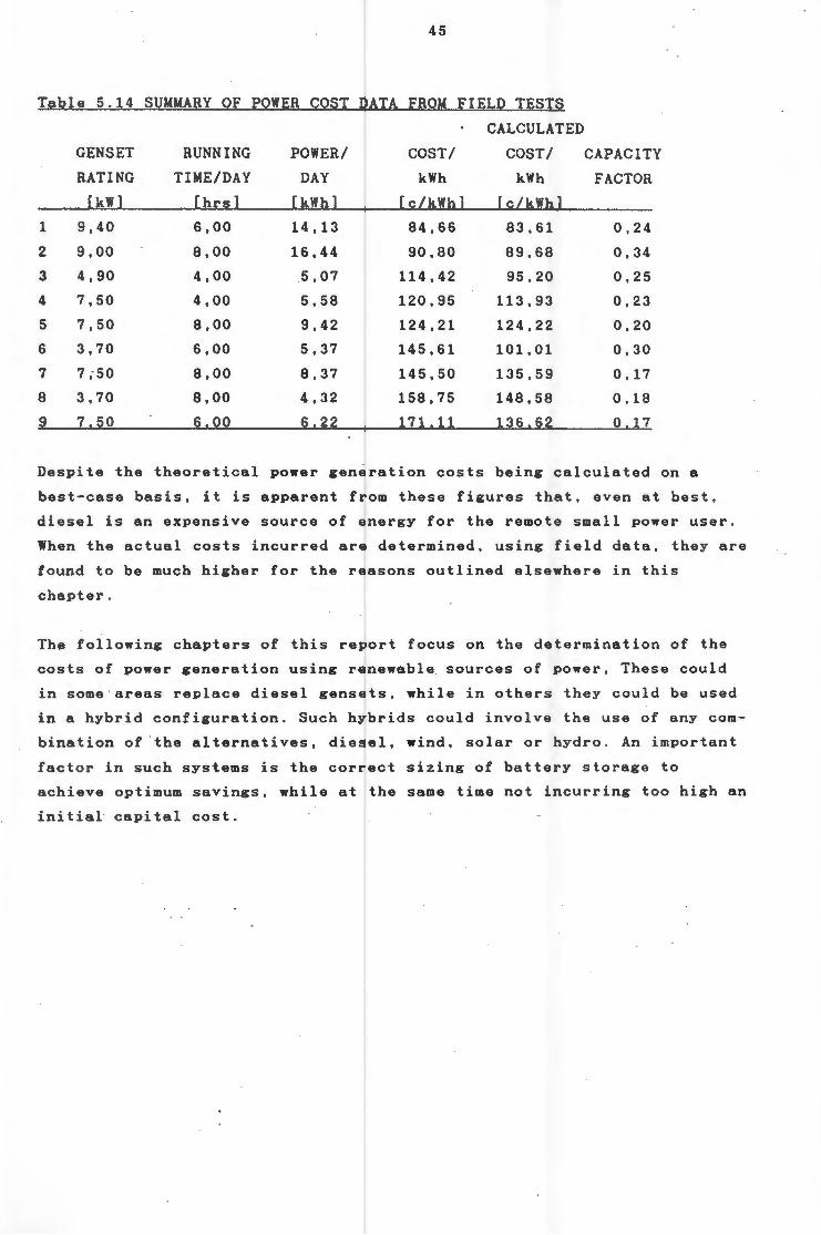
45
Table 5.14 SUMMARY OF POWER COST DATA FROM FIELD TESTS
CALCULATED
GENSET RUNNING POWER/ COST/ COST/ CAPACITY
1
2
3
4
5
6
7
8
9
RATING
[kW]
9,40
9,00
4,90
7,50
7,50
3,70
7;50
3,70
7.50
TIME/DAY
[hrsl
6,00
8,00
4,00
4,00
8,00
6,00
8,00
8,00
6,00
DAY
[kWh)
14,13
16,44
5,07
5,58
9,42
5,37
8,37
4,32
6.22
kWh
[c/kWh)
84,66
90,80
114 '42
120,95
124,21
145,61
145,50
158,75
171.11
kWh
[c/kWh]
83,61
89,68
95,20
113 '93
124,22
101,01
135,59
148,58
136,62
FACTOR
0,24
0,34
0 , 25
0,23
0,20
0,30
0,17
0,18
0 . 17
Despite the theoretical power generation costs being calculated on a
best-case basis, it is apparent from these figures that, even at best,
diesel is an expensive source of energy for the remote small power user.
When the actual costs incurred are determined, using field data, they are
found to be much higher for the reasons outlined elsewhere in this
chapter.
The following chapters of this report focus on the determination of the
costs of power generation using renewable. sources of power, These could
in some areas replace diesel gensets, while in others they could be used
in a hybrid configuration. Such hybrids could involve the use of any com
bination of the alternatives, diesel, wind, solar or hydro. An important
factor in such systems is the correct sizing of battery storage to
achieve optimum savings, while at the same time not incurring too high an
initial capital cost.
46
CHAPTER SIX
SOLAR POWER GENERATION
The amount of solar energy received by the earth in only one hour is
about equal to the total world energy consumption in one year . How
ever, only a small fraction of this can be effectively utilised . The
most obvious and simplest use of solar energy is to convert it into
heat via a thermal solar collector. Thus it is understandable that
early developments .of solar·energy systems concentrated on the use of
solar energy to supplement domestic space and water heating.
More recently, the conversion of sunlight to electricity has captured
the interest of many scientists and engineers. This has promise as an
effective decentralized power generation system, and can basically be
achieved through two fundamentally different methods - solar thermal
and photovoltaic. Naturally, because of the need for power at times
when there is no insolation, all solar power generation systems
require some form of storage, usually in the form of chemical or
thermal energy.
6 . 1 SOLAR ELECTRICAL POWER GENERATION TECHNOLOGIES
6.1.1 Solar Thermal
Generation of electrical power from solar thermal energy is achieved
by concentrating the sunlight onto an absorber , so as to produce a
high-temperature fluid ranging in temperature from 100-1700°C. This
fluid is then used to power a Carnot cycle engine, such as a Rankine
engine, and thereby generate electricity. The concentration of sun
light is achieved either through central or distributed receivers. In
a central receiver system, heliostats, or sun-tracking reflectors
direct the sun's rays at a central receiver which absorbs the
concentrated sunlight and transfers it as heat to a circulating
working fluid.
A distributed receiver system consists of one of two types of
collector. Parabolic line-focus or trough reflectors focus sunlight
onto a linear receiver tube positioned along the focal line of the
47
trough. A circulating heat transfer fluid in the tube transports the
heat energy to the point of use via a network of pipes.
Parabolic dish systems use point-focusing concentrating reflectors up
to 11m in diameter that focus the sunlight onto a receiver at the
focal point of the concentrator. These dish modules can be used alone
or in a multimodule system. The heat generated can then be used by a
heat engine coupled directly to the individual dishes, or else a
circulating fluid is used to convey the energy to a central point for
use.
Solar thermal power generation is being investigated in Israel, the
USA, Japan, France, Spain and Australia. The first large scale semi
commercial facility, Solar One, a 10 MWe facility in Southern
California, came on line in April 1982, and has achieved a maximum
energy delivery in one day of 104 MWh. This central receiver facility
has served very well as a proof of concept test. Costs for similar
plant have _dropped dramatically as a result of the experience gained
with this project, in particular as regards the technology for the
heliostats. However, the initial capital costs of these systems are
higher than those of the distributed collector systems. Thus they are
not well suited to small-scale applications. They are, however, being
~ursued as the commercial option for utility-scale power generation,
as they have higher overall efficiencies, and are thus cheaper over a
say 30-year life cycle.
Looking now at distributed collector technology, both parabolic trough
and parabolic dish reflectors are well demonstrated and proven. Trough
reflectors are used to produce the process heat for centrally-located
generating facilities, while the dish is the technology best suited to
small-scale application, with an individual Stirling engine per dish.
This is a technology that has been taken to commercialization by the
McDonnell Douglas Corporation who have developed a 25 kW Dish/Stirling
in collaboration with United Stirling AB of Sweden. This system has a
conversion effi~iency of sunlight to electricity of 28%. It also has
the advantage of modularity and the system output can be increased
with the introduction of additional units.
Luz Industries, an Israeli company, and its Californian operation, Luz
International have become leaders in the development of parabolic
trough technology. The third and fourth of their solar electric
48
generating systems (SEGS) both came on line in December 1986 in the
Mojave Desert, California, and have a combined net output of 60 MWe .
Another two 30 MWe plants are currently under construction and dew to
come on line towards the end of 1987. SEGS VII will be the last to be
constructed under the favourable power purchase contracts made
available in California, and will come on line in early 1988 . An
additional 12 contracts have been sealed for implementation after 1988
(SEIR, 1987). The cost per kilowatt of these plants has dropped
steadily with each successive installation, from SEGS I at US$ 4500/kW
to SEGS III at US$ 3466/kW and SEGS IV at US$ 3366/kW . (These are
1983, 1986 and 1986 prices respectively. Adjustment of the 1983 price
to present day US$ would therefore represent an even greater reduction
per kW).
In Australia a number of small systems are being investigated in
demonstration experiments. The largest of these is a hybrid solar/
diesel power plant at Meekatharra. The technology being used is that
of the German company M. A. N. In the past power was provided by a
multi-engine diesel-powered station with a peak output of 800 kW. This
is now being supplemented by 100 kW of peak power - 50 kW from the
solar plant and 50 kW from diesel exhaust heat recovery. The collector
field consists of 960 m1 of parabolic trough concentrators. The heat
from this and the exhaust recovery system is then used to generate
steam which drives a two-stage, wet operation screw expansion engine.
The level of technical backup has been high thusfar, and the real
practical test of the system will come when it is operated solely by
the existing diesel plant personnel.
Another small-scale Australian project is the White Cliffs Solar Power
Station. This plant produces 25 kW power and comprises 14 modular
semi-autonomous parabolic dish collectors. Steam is generated by these
collectors and conveyed to a high performance reciprocating uniflow
steam engine which converts it to mechanical power at a heat to work
conversion efficiency of 22%. This power is then used to drive an
AC/DC set, the alternator feeding the load, while any excess output is
fed into battery storage. In times of low or zero insolation this DC
power is used to drive the DC machine which in turn drives the alter
nator to supply the load . A backup diesel is also available in the
event of total failure. A second stage of this scheme is to provide
water to the town through the use of waste low-grade heat for desal
ination. The total system has proved robust and manageable, and
49
studies have been undertaken on smaller systems suitable for serving
single households (Eberhard, 1983).
Since 1981, overall momentum in the development of solar thermal power
generation technology ~as slowed, mainly as a result of lower fossil
fuel prices, and the cut in US expenditure on research into energy
al t ernatives (SEIA, 1986). This technology is not yet being used
commercially for small remote power applications.
6 . 1.2 Solar Photovoltaic
Photovoltaic (PV) or solar cells are semiconductor devices that
convert photons of incident sunlight directly into DC electricity.
These have been used in space programmes since 1958 , to provide power
for orbiting satellites. These cells are efficient at converting
sunlight into electricity, of the order of 20%. However their cost
makes them very expensive for use on the earth . In some ways the
entire research programme for solar cell development has been directed
at taking this proven technology and making it cheaper.
A solar cell typically consists of two different types of semi
conductor material, called n-type and p-type . Energy carried by the
\ncident photons frees positive and negative charges within the cell
materials. The junction between the n- and p-type materials creates an
electric field, causing the freed charges to separate across the
junction and thus create a voltage across the cell . Electric contacts
placed on the two sides of the cell allow the current generated by
th i s potential to be applied to an external load.
The amount of electric current generated by a cell is primarily
dependent on the intensity of solar radiation striking its exposed
a r ea. The open-circuit voltage produced, however, is primarily
depenqent on the temperature of the cell, voltage and cell temperature
being inversely related.
Because the power output of a single solar cell is small (1 Watt for a
typical cell of 100 cm1, 10% efficiency), a number of cells are
usually connected in series and parallel, and sold as a module . These
in turn can be wired together into an array, to generate the amount of
power required by the application. Efficiencies being achieved in the
laboratory with the latest materials are up at 28%, although many of
the new thin-film cells are still close to 10% (Zweibel, 1986).
50
New technologies are however being pursued, amongst them amorphous
silicon (a-Si) , copper indium diselenide, cadmium telluride and
gallium arsenide. All of these materials are being considered for f l at
plate applications. Gallium arsenide (GaAs) and thick crystalline
silicon are being developed as candidates for concentrator
applications, using optical lenses or reflectors·. In this way the cos t
of relatively expensive solar cells is offset by the less expensive
enhancing optics. Another strategy for enhancement is based on the so
called cascade or multi-junction cells. These consists of a stack of
cells atop one another so that the sun's spectrum is used more
effectively (Zweibel, 1986).
The two most important variables determining the economic competitive
ness of PV modules are their cost per square metre and efficiency of
conversion. The US Dept of Energy has determined that unless module
cost can be driven below US$ 40/m', efficiencies of about 15% will be
needed for economical production (Zweibel, 1986) . The more expensive
but mature technologies, crystalline Si and GaAs have efficiencies of
~ver 20-25%, but high costs, of the order of US$ 900 - 1000/m 2 •
This technology provides a potentially cost-effective alternative to
~onventional power sources in a variety of remote applications, where
the operation, maintenance, and fuel costs of the conventional sources
are high. PVs can be used to provide either AC or DC power, the former
requiring the inclusion of some fairly sophisticated electronic
equipment in the system.
PVs have already been used extensively in South Africa and Namib i a to
provide power for telecommunications, in both radio and telephone
repeater stations. Other installations which have been erected in the
past year are a large number of audio-visual education facilities in
rural areas of Bophutatswana and the Ciskei. Other appropriate appli
cations with near term applicability are refrigeration at remote
clinics and water pumping.
The PV System
A practical stand-alone PV power system typically requires several
elements . in addition to the array in order to satisfy the intended
load. This equipment includes what is often referred to as the balance
of system (BOS) i.e. support structures, fencing and other
51
infrastructural requirements, and ancillary equipment for power
storage and conditioning.
Power storage, most commonly involving a lead-acid battery in present
applications, stores electrical energy produced during daylight hours
for use during the night or during periods of reduced insolation. To
be considered practical for remote applications, a storage battery
should have a long life, require low maintenance, and be able to
survive~ substantial number of deep discharge cycles.
An important component of a power system using storage is a voltage
regulator wh±ch controls the output voltage from the array when it is
charging the battery. The regulator also li.mits the loss of water from
the battery cells. This can occur during periods of gassing if charge
rates are kept too high once the battery is fully charged.
6.2 THE POTENTIAL FOR SOLAR POWER GENERATION IN SOUTH AFRICA
Insolation characteristics important for assessing the potential for
solar power generation include the following: diurnal variation,
regional and seasonal variability, and weather.
6.2.1 Diurnal Variation
The most important char•cteristic of {nsolation when considering the
use .of solar energy is its diurnal pattern, i.e. its variation over
the period of a day. The expected solar power available to a solar
powered device, over a 24-hour period, under clear sky conditions,
will follow a curve similar to that in the following figure.
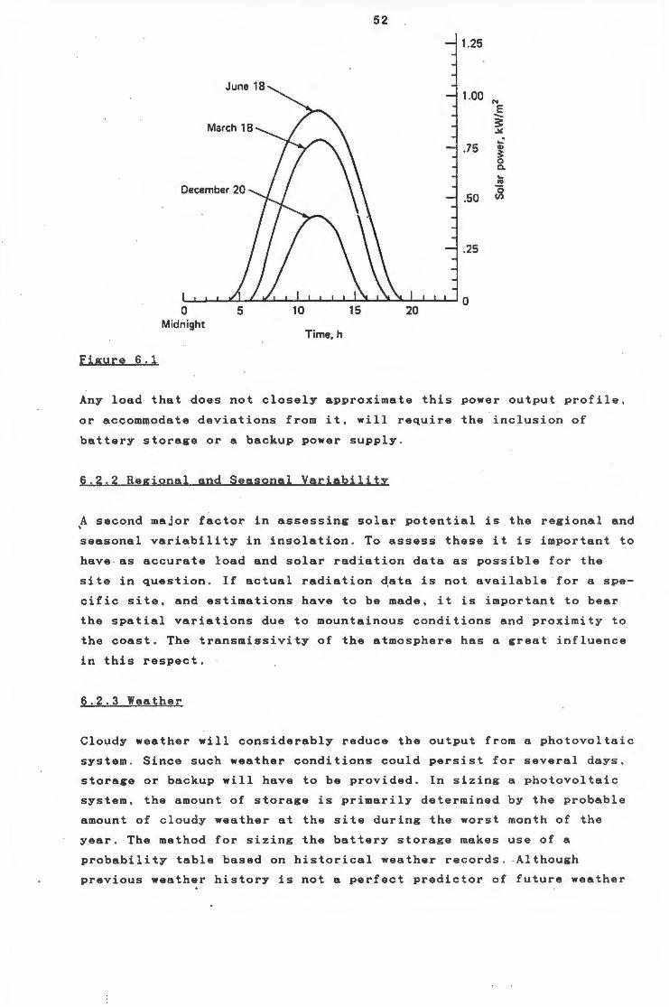
Figure 6.1
0 Midnight
5 10
52
15 20
Time,h
1.25
1.00 N
E ..... 3 ~
.. : .75 Ql
~ 0 c. .... Ill
0 .50 (I)
.25
Any load that does not closely approximate this power output profile ,
or accommodate deviations from it, will require the inclusion of
battery storage or a backup power supply .
6.2.2 Regional and Seasonal Variability
A second major factor in assessing solar potential is the regional and
seasonal variability in insolation . To assess these it is important to
have as accurate load and solar radiation data as possible for the
site in question. If actual radiation ~ata is not available for a spe
cific site, and estimations have to be made, it is important to bear
the spatial variations due to mounta i nous c onditions and proximi ty to
the coast. The transmissivity of the atmosphere has a great influence
in this respect.
6.2.3 Weather
Cloudy weather will considerably reduce the output from a photovoltaic
system. Since such weather conditions could persist for several days,
storage or backup will have to be provided. In sizing a photovoltaic
system, the amount of storage is primarily determined by the probable
amount of cloudy weather at the site during the worst month of t he
year. The method for s i zing the battery storage makes use of a
probability table based on historical weather records . . Although
previous weather history is not a perfect predictor of future weather
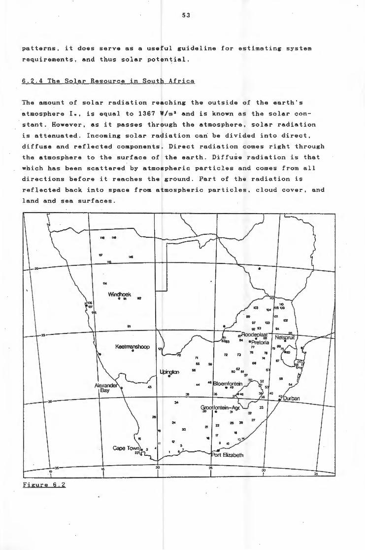
53
pa t terns , it does serve as a useful guideline for estimating system
req uirements, and thus solar potential .
6 . 2 . 4 The Solar Resource in South Africa
The amount of solar radiation reaching the outside of the earth's
a t mosphere I., is equal to 1367 W/m 2 and is known as the solar con
s t ant. However, as it passes through the atmosphere, solar radiation
is attenuated. Incoming solar radiation cari be divided into direct,
di f fuse and reflected components . Direct radiation comes right through
the atmosphere to the surface of the earth . Diffuse radiation is that
wh i ch has been scattered by atmospheric particles and comes from all
d irections before it reaches the ground. Part of the radiation is
reflected back into space from atmospheric particles, cloud cover, and
lan d and sea surfaces.
1111 lltl
117 I"'
Windhoek • m 10
91
F i gure 6.2
54
Systematic measurement of total and diffuse radiation received at the
earth's surface have been made by the SA Weather Bureau since 1951 .
There are currently fifteen stations recording solar radiation;
thirteen are in South Africa and two in Namibia, but only twelve of
these are recording useful data (these are named on the map shown in
Figure 6.2) . As can be seen these stations are located mostly along
the coast, where weather conditions vary much more than over the
interior plateau. The spatial distribution of sunshine measuring
stati~ns (indicated by numbers on the map) is however much better
(Tegen et al, 1988).
The ERI has embarked on a project to evaluate all the radiation data
available from ~he South African Weather Bureau and the Department of
Agriculture. The aim is to develop a handbook for solar installation
designers. One problem already mentioned is that these two sources do
not have enough radiation measurement stations to enable the drawing
of accurate isopyrs . It is apparent that their spatial distribution i s
not therefore ideal for the accurate determination of solar radiat i on
in many parts of the country.
However, in addition to solar radiation data, sunshine data is record
ed at over 150 locations, with a far better spatial distribution . This
data is being used to generate solar radiation data to enable interpo
lation between the solar radiation stations.
Figures 6.3 to 6.6 show global radiation in January , April, July and
October for South Africa (Tegen et al, 1988). These maps give an
indication of the seasonal variation that occurs . Dur j ng the summ e r
the values south of the Tropic of Capricorn are roughly twice those
during winter. It is interesting to note that solar radiation levels
increase towards the south . This phenomenon can be attributed to the
fact that although solar radiation levels are highest around the
equator at the atmosphere's outer surface, water vapour, dust and
similar aerosols cause higher levels of attentuation in humid tropical
and dry dusty regions.
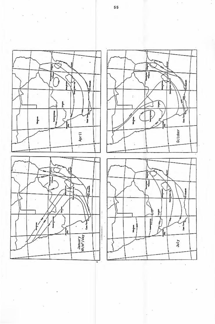
55
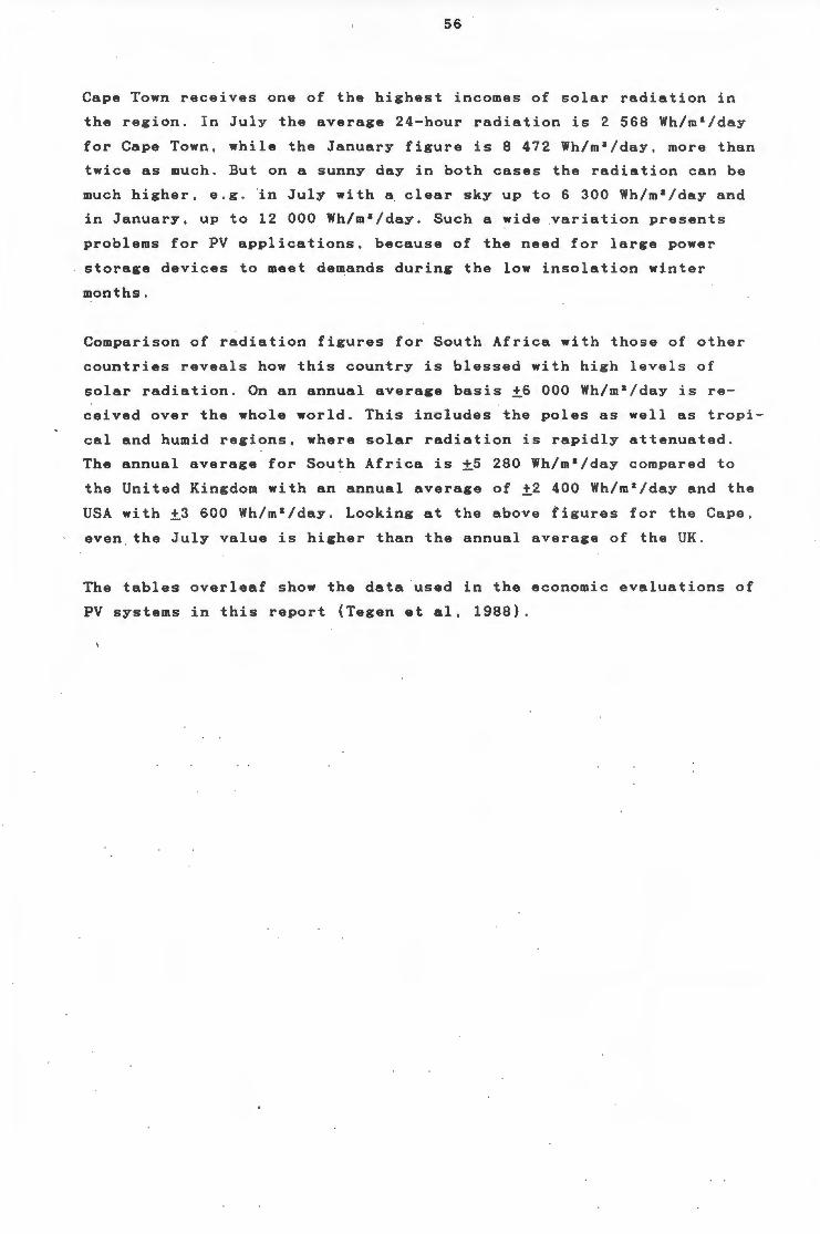
56
Cape Town receives one of the highest incomes of solar radiation in
the region. In July the average 24-hour radiation is 2 568 Wh/m 2 /day
for Cape Town, while the January figure is 8 472 Wh/m 2 /day, more than
twice as much. But on a sunny day in both cases the radiation can be
much higher, e.g . in July with ~clear sky up to 6 300 Wh/m 2 /day and
in January, up to 12 000 Wh/m 2 /day . Such a wide .variation presents
problems for PV applications, because of the need for large power
storage devices to meet demands during the low insolation winter
months .
Comparison of radiation figures for South Africa with those of other
countries reveals how this country is blessed with high levels of
solar radiation. On an annual average basis ±6 000 Wh/m 3 /day is re
ceived over the whole world . This includes the poles as well as tropi
cal and humid regions, where solar radiation is rapidly attenuated .
The annual average for South Africa is ±5 280 Wh/m 2 /day compared to
the United Kingdom with an annual average of ±2 400 Wh/m 2 /day and the
USA with ±3 600 Wh/m 2 /day . Looking at the above figures for the Cape ,
even . the July value is higher than the annual average of the UK .
The tables overleaf show the data used in the economic evaluations of
PV systems in this report (Tegen et al , 1988).
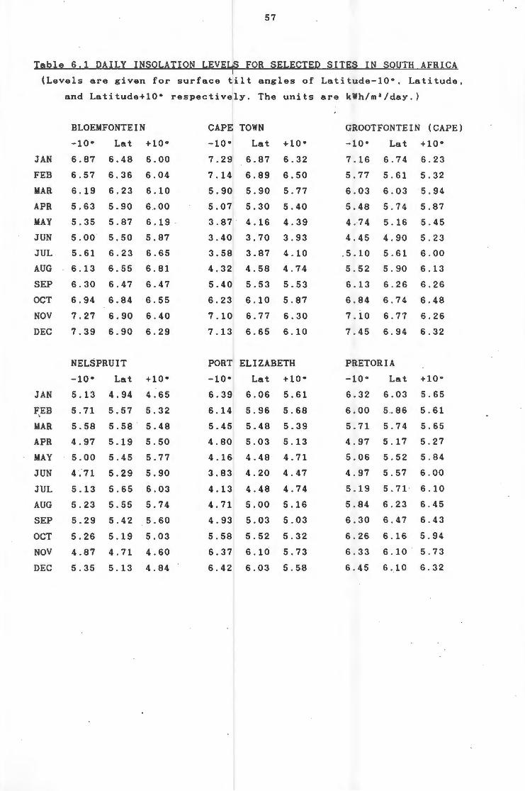
57
Table 6.1 DAILY INSOLATION LEVELS FOR SELECTED SITES IN SOUTH AFRICA
(Levels are given for surface tilt angles of Latitude-10•, Latitude,
and Latitude+10• respectively. The units are kWh/m 2 /day . )
BLOEMFONTEIN CAPE TOWN GROOTFONTEIN (CAPE)
-10• Lat +10• -10• Lat +10• -10• Lat +10•
JAN 6.87 6.48 6.00 7.29 6.87 6.32 7.16 6 . 74 6.23
FEB 6.57 6.36 6.04 7.14 6.89 6.50 5.77 5.61 5.32
MAR 6.19 6.23 6.10 5.90 5.90 5.77 6.03 6.03 5.94
APR 5.63 5.90 6 _.00 5.07 5.30 5.40 5 . 48 5.74 5.87
MAY 5.35 5.87 6.19 . 3.87 " 4.16 4.39 4.74 5.16 5.45
JUN 5.00 5.50 5.87 3.40 3.70 3.93 4.45 4 . 90 5 . 23
JUL 5.61 6.23 6.65 3.58 3.87 4 . 10 . 5 .10 5 . 61 6.00
AUG 6.13 6.55 6.81 4.32 4.58 4 . 74 5 . 52 5 . 90 6.13
SEP 6.30 6.47 6.47 5.40 5.53 5.53 6.13 6.26 6 . 26
OCT 6.94 6.84 6.55 6.23 6.10 5.87 6 . 84 6 . 74 6.48
NOV 7.27 6.90 6.40 7.10 6.77 6.30 7.10 6.77 6.26
DEC 7.39 6.90 6.29 7.13 6.65 6.10 7.45 6.94 6.32
NELSPRUIT PORT ELIZABETH PRETORIA
-10• Lat +10• -10• Lat +10• -10° Lat +10•
JAN 5.13 4.94 4.65 6.39 6.06 5.61 6.32 6.03 5.65
FEB 5.71 5.57 5.32 6.14 5.96 5.68 6.00 5.86 5.61 \
MAR 5.58 5.58 5.48 5.45 5.48 5.39 5.71 5 . 74 5.65
APR 4.97 5.19 5.50 4.80 5.03 5.13 4.97 5.17 5 . 27
MAY 5.00 5.45 5.77 4.16 4.48 4.71 5 . 06 5 . 52 5.84
JUN 4.71 5.29 5.90 3.83 4.20 4.47 4.97 5.57 6.00
JUL 5.13 5.65 6.03 4.13 4.48 4.74 5 . 19 5 . 71 6.10
AUG 5.23 5.55 5.74 4.71 5.00 5.16 5 . 84 6.23 6.45
SEP 5.29 5.42 5.60 4.93 5.03 5.03 6.30 6.47 6.43
OCT 5.26 5.19 5.03 5.58 5.52 5.32 6 . 26 6.16 5.94
NOV 4.87 4.71 4.60 6.37 6.10 5.73 6.33 6.10 5.73
DEC 5.35 5 . 13 4.84 6.42 6.03 5.58 6 . 45 6.10 6.32
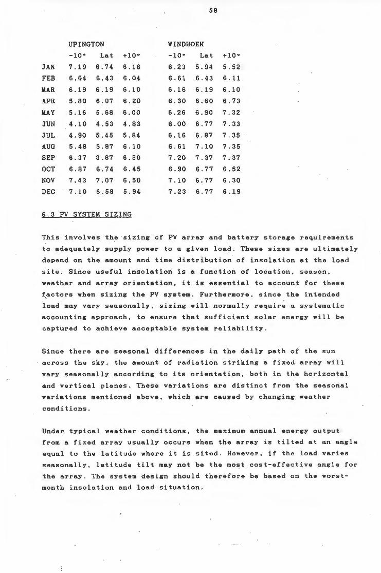
58
UPINGTON WINDHOEK
-10° Lat +10° -10° Lat +10°
JAN 7.19 6.74 6.16 6.23 5.94 5.52
FEB 6.64 6.43 6.04 6.61 6.43 6 . 11
MAR 6.19 6.19 6.10 6.16 6.19 6.10
APR 5.80 6.07 6.20 6.30 6.60 6.73
MAY 5.16 5.68 6.00 6.26 6.90 7.32
JUN 4.10 4.53 4.83 6.00 6 . 77 7.33
JUL 4.90 5.45 5.84 6.16 6 . 87 7 . 35
AUG 5.48 5 . 87 6.10 6.61 7 . 10 7.35
SEP 6 . 37 3.87 6.50 7.20 7 . 37 7.37
OCT 6.87 6.74 6.45 6.90 6.77 6.52
NOV 7.43 7.07 6.50 7.10 6 . 77 6.30
DEC 7.10 6.58 5.94 7.23 6.77 6.19
6.3 PV SYSTEM SIZING
This involves the sizing of PV array and battery storage requirements
to adequately supply power to a given load. These sizes are ultimately
depend on the amount and time distribution of insolation at the load
site. Since useful insolation is a function of location, season ,
weather and array orientation, it is essential to account for these
f ,actors when sizing the PV system. Furthermore, since the intended
load may vary seasonally , sizing will normally require a systematic
accounting approach, to ensure that sufficient solar energy will be
captured to achieve acceptable system reliability.
Since there are seasonal differences in the daily path of the sun
across the sky, the amount of radiation striking a fixed array will
vary seasonally according to its orientation, both in the horizontal
and vertical planes. These variations are distinct from the seasonal
variations mentioned above, which are caused by changing weather
conditions.
Under typical weather conditions, the maximum annual energy output
from a fixed array usually occurs when the array is tilted at an angle
equal to the latitude where it is sited. However, if the load varies
seasonally, latitude tilt may not be the most cost-effect ive angle for
the array. The system design should therefore be based on the worst
month insolation and load situation.
59
The Solar Energy Research Institute (SERI) of the USA has developed a
PV system sizing methodology which takes the above into consideration
(Borden et al, 1984) .· In addition it has built into it the concept of
Loss of Energy Probability (LOEP). This allows for the sizing of the
PV system and its battery storage so as to provide power with a degree
of certainty as described by the LOEP. This methodology has been used
in the following section, with an LOEP of 0,1 i . e. there is a 10%
probability that the system will not be able to supply the required
power at any time. This is equivalent to the LOEP of a diesel powered
generator, which would in most cases be the alternative to a PV
system. The method involves the calculation of two sizing factors, S.
and s~ . which refer to the array and the battery storage bank, and
have the units of kWh/ma/day and days, respectively.
6 . 4 THE ECONOMICS OF PV GENERATED POWER
The economics of photovoltaic generated power is dominated by the high
in i tial capital cost of the equipment. Despite the sustained efforts
of cell manufacturers to bring their costs down, they are still not
competitive with diesel power generation in many remote applications.
This has been further aggravated locally by the decline in the value
of the Rand relative to the US Dollar. When photovoltaic cells were
~irst produced in 1959 they cost of the order of US$1 000 per peak
Watt (Wp). This price has been steadily decreasing over the past
th i rty years with 1987 prices now around US$5. However, the South
_African retail price is still of the order of R20 per Wp. Predictions
are that by 1995 cells will be costing around US$2-3,50 per Wp.
Using the system sizing methodology outlined in the previous section,
the economics of remote PV power generation has been investigated for
a number of sites in South Africa and Namibia. A number of different
system specifications have been used, along with the general assump
tions and data as follows:
Table 6 . 2 SYSTEM CHARACTERISTICS AND COST DATA
Syste~ life
Discount rate (reall
Escalation rate (real)
25.00 years
5.00%
0.00%
PV MODULES
Module cost
Module efficiency
Module operating temperature
Module temp coefficient
Balance of System (% of capital cost)
O&M cost (% of capital cost)
VOLTAGE REGULATOR
Voltage regulator efficiency
Cost
BATTERIES
Battery efficiency
Depth of discharge
Battery type
Battery life
Cost R/kWh
O&M cost (% of capital cost)
INVERTER
Inverter efficiency
Cost R/Wac \
60
R20.00 /pW
12 . 00%
60 . 00 oc -0 . 0050 Joe 0.05%
1.00%
95 . 00%
RlOOO.OO
90.00%
50.00%
(Tubular/Traction/Automotive)
10.00 years
Dependent on type
5.00%
80.00%
R1 . 34 /Wac
In all the following tables, the total installed cost referred to
includes the capital cost of the solar module array, BOS, all energy
storage and power conditioning equipment, and its installation.
The basic specifications of the first system which is evaluated at a
· number of sites and comprises a small domestic load , are:
Peak load
Daily consumption
AC loads?
Induction loads?
4.00 kVA
10 . 35 kWh/day
YES
YES
As far as the inductive loads are concerned, they will affect the size
of inverter required to provide the necessary starting current. The
following are the sites at which it is evaluated: Bloemfontein (BFN) ,
Cape Town (CTA), Grootfontein Agricultural Station in the Cape (GFN),
Port Elizabeth (PLZ), Nelspruit (NEL), Pretoria (PTA), Windhoek (WHK),
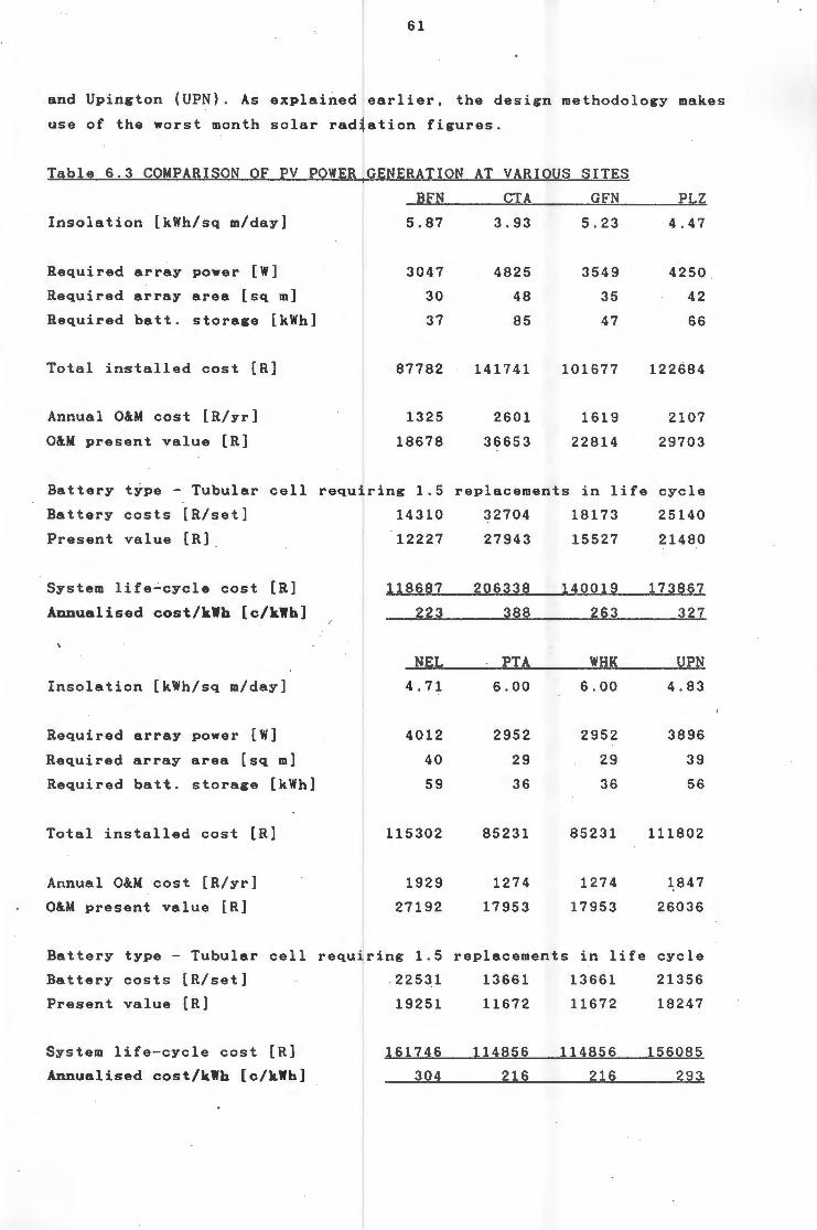
61
and Upington (UPN). As explained earlier, the design methodology makes
use of the worst month solar radiation figures.
Table 6.3 COMPARISON OF PV POWER GENERATION AT VARIOUS SITES
Insolation [kWh/sq m/day]
Required array power [W]
Required array area [sq m]
Required batt. storage [kWh]
Total installed cost [R]
Annual O&M cost [R/yr]
O&M present value [R]
BFN
5.87
3047
30
37
87782
1325
18678
CTA
3.93
4825
48
85
141741
2601
36653
GFN
5 . 23
3549
35
47
101677
1619
22814
PLZ
4.47
4250
42
66
122684
2107
29703
Battery type -Tubular cell requiring 1.5 replacements in life cycle
Battery costs [R/set]
Present value [R]
System life~cycle cost [R]
Annualised cost/kWh [c/kWh]
Insolation [kWh/sq m/day]
Required array power [W]
Required array area [sq m]
Required batt. storage [kWh]
Total installed cost [R]
Annual O&M cost [R/yr]
O&M present value [R]
Battery type - Tubular
Battery costs [R/set]
Present value [R]
System life-cycle cost
cell
[R]
Annualised cost/kWh [c/kWh]
14310
12227
118687
223
NEL
4.71
4012
40
59
115302
1929
27192
requiring 1.5
. 22531
19251
161746
304
32704
27943
206338
388
PTA
6.00
2952
29
36
85231
1274
17953
18173
15527
140019
263
WHK
6.00
2952
29
36
85231
1274
17953
replacements in life
13661 13661
11672 11672
114856 114856
216 216
25140
21480
173867
327
UPN
4.83
3896
39
56
111802
1847
26036
cycle
21356
18247
156085
293.
62
It is apparent from the foregoing that the unit cost of PV generated
power is very much dependent on the worst insolation level prevailing
at a site. Thus it can be seen that Cape Tow~ which over the year
receives a substantial amount of solar radiation, in fact one of the
high~st totals in the region, nonethel~ss has the most expensive PV
generated power. This is of course attributable to the fact that to
ensure acceptable power supply during the winter months , both a larger
solar module array and battery bank are required . The battery bank is
in fact 8,5 times the daily power consumption of the system .
In order to get a better idea of the cost of PV power supply, a number
of other systems were evaluated. These evaluations were all based on
the solar radiation levels measured at Grootfontein Agricultural
Research Station in the Eastern Cape. This site was chosen ,because of
its proximity to a number of areas which could eventually become users
of alternative power generation technologies .
The first three systems are all supplying domestic loads of the type
currently supplied by diesel gensets. The systems have therefore been
sized in order to supply AC loads and the assumption is made that
there are induction motors being used for refrigerators and other
a~pliances. Thus allowance is made for the provision of starting
current levels of three times the peak.
The batteries specified in these comparisons are all of the tubular
cell type. They are therefore the most expensive option, but are
claimed by the manufacturers to provide the lowest maintenance and
longest service life characteristics .
It is of interest to note that the peak demand has less effect on the
system cost than does the daily power consumption. However, the higher
consumption has the effect of improving the overall utilisation of the
system thus resulting in a lower cost per unit of power. Indeed the
system with the highest overall life-cycle cost produces the cheapest
power. This highlights the necessity for very careful design of
systems comprising such capital intensive equipment .
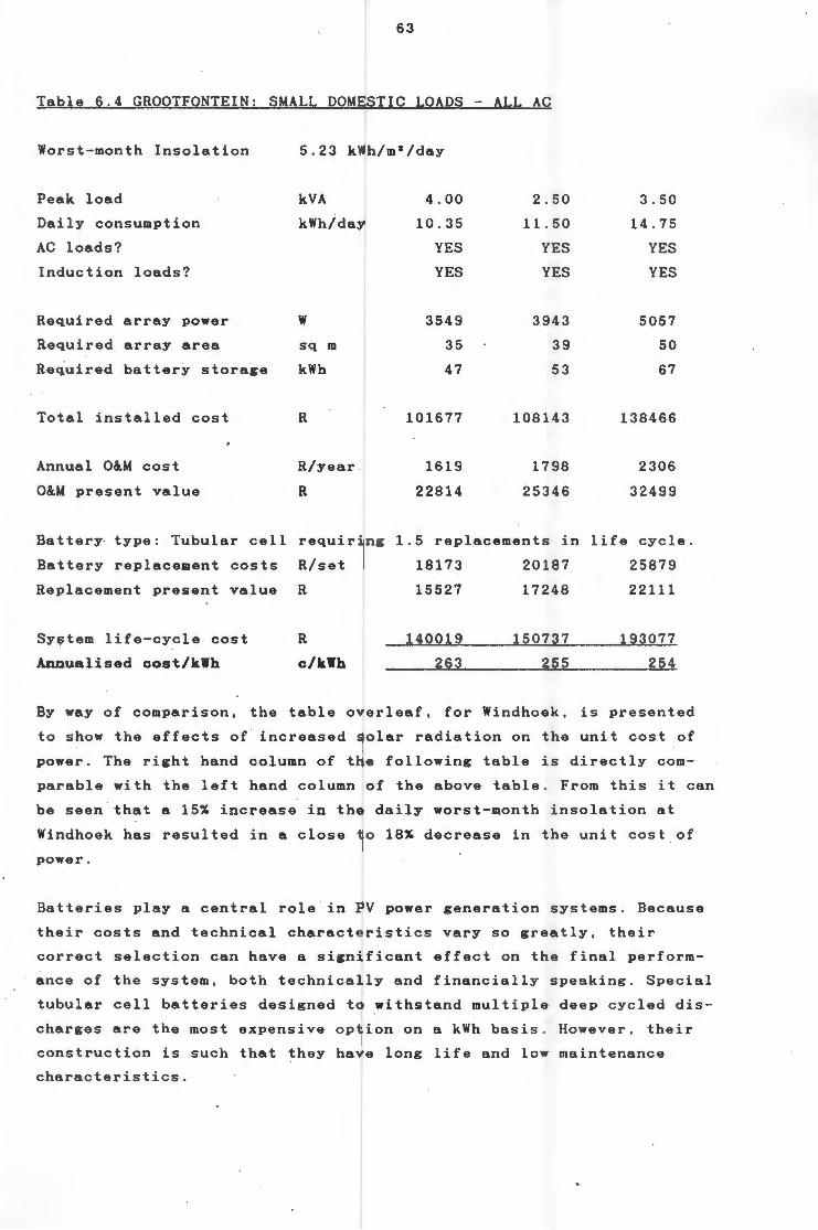
63
Table 6 . 4 GROOTFONTEIN: SMALL DOMESTIC LOADS - ALL AC
Worst-month Insolation
Peak load
Daily consumption
AC loads?
Induction loads?
Required array power
Required array area
Required battery storage
Total installed cost
Annual O&M cost
O&M present value
5.23 kWh/m 3 /day
kVA
kWh/day
w sq m
kWh
R
R/year
R
4.00
10.35
YES
YES
3549
35
47
101677
1619
22814
2 .5 0
11 .5 0
YES
YES
3943
39
53
108143
1798
25346
3 . 50
14.75
YES
YES
5057
50
67
138466
2306
32499
Battery· type: Tubular cell requiring 1.5 replacements in life cycle.
Battery replacement costs R/set 18173 20187 25879
Replacement present value R 15527 17248 22111
Sy~tem life-cycle cost
Annualised cost/kWh
R
c/kWh
140019
263
150737 193077
255 254
By way of comparison, the table overleaf, for Windhoek, is presented
to show the effects of increased solar radiation on the unit cost of
power. The right hand column of the following table is directly com
parable with the left hand column of the above table . From this it can
be seen that a 15% increase in the daily worst-month insolation at
Windhoek has resulted in a close to 18% decrease in the unit cost of
power .
Batteries play a central role in PV power generation systems. Because
their costs and technical characteristics vary so greatly, their
correct selection can have a significant effect on the final perform
ance of the system, both technically and financially speaking. Special
tubular cell batteries designed to withstand multiple deep cycled dis
charges are the most expensive option on a kWh basis. However, their
construction is such that they have long life and low maintenance
characteristics.
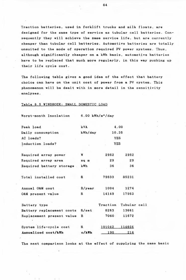
64
Traction batteries, used in forklift trucks and milk floats, are
designed for the same type of service as tubular cell batteries . Con
sequently they will achieve the same service life, but are currently
cheaper than tubular cell batteries. Automotive batteries are totally
unsuited to the mode of operation required PV power systems. Thus,
although significantly cheaper on a kWh basis, automotive batteries
have to be replaced that much more regularly, in this way pushing up
their life cycle cost.
The following table gives a good idea of the effect that battery
choice can have on the unit cost of power from a PV system. This
phenomenon will be dealt with in more detail in the sensitivity
analyses.
Table 6.5 WINDHOEK: SMALL DOMESTIC LOAD
Worst-month Insolation
Peak load
Daily consumption
AC loads?
Induction loads? . Required array power
Required array ·area
Required battery storage
Total installed cost
Annual O&.M cost
O&.M present value
Battery type
Battery replacement costs
Replacement present value
System life-cycle cost
Annualised cost/kWh
6.00 kWh/m 1 /day
kVA
kWh/day
w sq m
kWh
R
R/year
R
R/set
R
R
c/kWh
4 . 00
10.35
YES
YES
2952
29
36
79833
1004
14149
2952
29
36
85231
1274
17953
Traction Tubular
8263 13661
7060 11672
101042 114856
190 216
cell
The next comparison looks at the effect of supplying the same basic
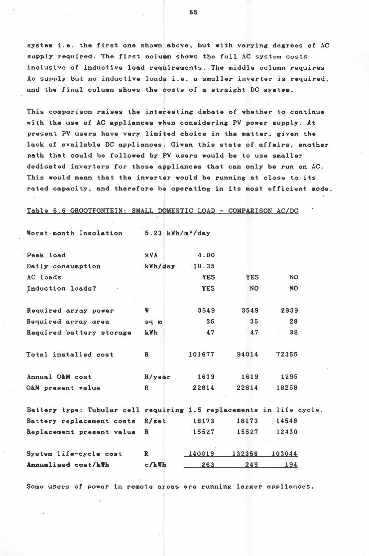
65
system i.e. the first one shown above, but with varying degrees of AC
supply required. The first column shows the full AC system costs
inclusive of inductive load requirements. The middle column requires
Ac supply but no inductive loads i.e. a smaller inverter is required,
and the final column shows the costs of a straight DC system.
This comparison raises the interesting debate of whether to continue
with the use of AC appliances when considering PV power supply. At
present PV users have very limited choice in the matter, given the
lack of available DC appliances. Given this state of affairs, another
path that could be followed by PV users would be to use smaller
dedicated inverters for those appliances that can only be run on AC.
This would mean that the inverter would be running at close to its
rated capacity, and therefore be operating in its most efficient mode.
Table 6 . 6 GROOTFONTEIN: SMALL DOMESTIC LOAD- COMPARISON AC/DC
Worst-month Insolation
Peak load
Daily consumption
AC loads
Induction loads? . Required array power
Required array area
Required battery storage
Total installed cost
Annual O&.M cost
O&.M present value
5.23 kWh/m 3 /day
kVA
kWh/day
w sq m
kWh
R
R/year
R
4.00
10.35
YES
YES
3549
35
47
101677
1619
22814
YES
NO
3549
35
47
94014
1619
22814
Battery type: Tubular cell requiring 1.5 replacements
Battery replacement costs R/set 18173 18173
Replacement present value R 15527 15527
System life-cycle cost
Annualised cost/kWh
R
c/kWh
140019
263
132356
249
NO
NO
2839
28
38
72355
1295
18258
in life cycle.
14548
12430
103044
194
Some users of power in remote areas are running larger appliances,
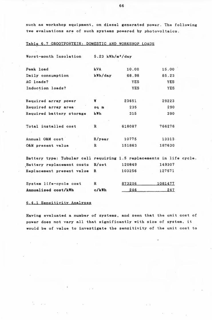
66
such as workshop equipment, on diesel generated power . The following
tw~ evaluations are of such systems powered by photovoltaics .
Table 6.7 GROOTFONTEIN: DOMESTIC AND WORKSHOP LOADS
Worst-month Insolation
Peak load
Daily consumption
AC loads?
Induction loads?
Required array power
Required array area
Required battery storage
Total installed cost
Annual O&.M cost ·
O&.M present value
5.23 kWh/m 2 /day
kVA
kWh/day
w sq m
kWh
R
R/year
R
10 . 00
68 . 98
YES
YES
23651
235
315
618087
10775
151863
15 . 00
85 . 23
YES
YES
29223
290
390
766276
13313 .
187630
Battery type: Tubular cell requiring
,Battery replacement costs R/set
Replacement present value R
1 . 5 replacements in life
120849 149307
103256 127571
System life-cycle cost R 873206 1081477
Annualised cost/kWh c/kWh 246 247
6.4.1 Sensitivity Analyses
cycle.
Having evaluated a number of systems, and seen that the unit cost of
power does not vary all that significantly with size of system, it
would be of value to investigate the sensitivity of the unit cost to
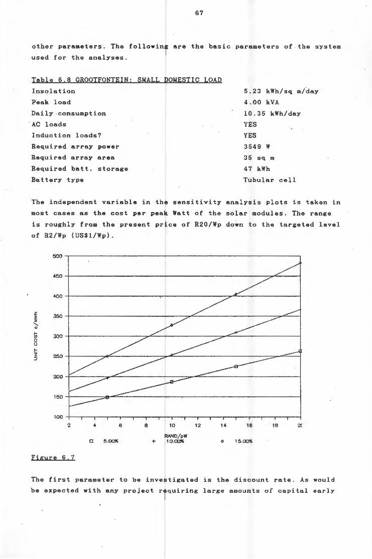
67
other parameters. The following are the basic parameters of the system
used for the analyses.
Table 6.8 GROOTFONTEIN: SMALL DOMESTIC LOAD
Insolation
Peak load
Daily consumption
' AC loads
Induction loads?
Required array power
Required array area
Required batt. storage
Battery type
5.23 kWh/sq m/~ay
4 . 00 kVA
10.35 kWh/day
YES
YES
3549 w 35 sq m
47 kWh
Tubular cell
The independent variable in the sensitivity analysis plots is taken in
most cases as the cost per peak Watt of the solar modules. The range
is roughly from the present price of R20/Wp down to the targeted level
of R2/Wp (US$1/Wp).
400
~ 350
' u .....
300 VI 0 u !:: z 250 ::>
200
2
a 5 .0~
Figure 6 . 7
6 8 10
RAND/pW + 10.~
12 14 16 18
0 15.~
The first parameter to be investigated is the discount rate. As would
be expected with any project requiring large amounts of capital early
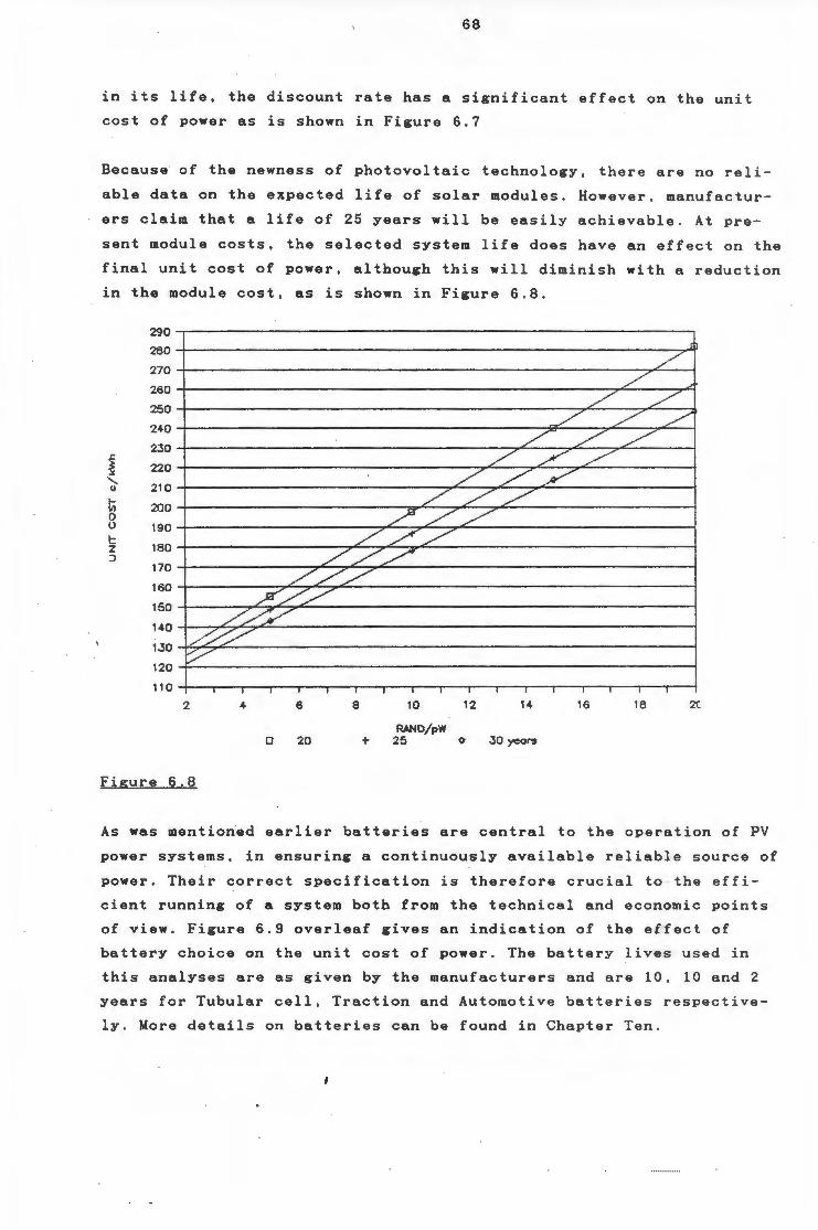
68
in its life, the discount rate has a significant effect on the unit
cost of power as is shown in Figure 6.7
Because of the newness of photovoltaic technology, there are no reli
able data on the expected life of solar modules. However, manufactur
ers claim that a life of 25 years will be easily achievable . At pre
sent module costs, the selected system life does have an effect on the
final unit cost of power, although this will diminish with a reduction
in the module cost, as is shown in Figure 6.8 .
290
280
270
260
250
240
230
~ 220 "' ' 210 u
Iii 200 0 u 190 !:::
180 z :J
170
160
150
140
130
120
/ L
L L L L L_
L LL / //
LLL_ LLL
/// //L_
//~ _,///
/_/_/ ~-:/---
/~/ v
110
2 4 6 8 10 12 14 16 18 2C
RAND/pW 0 20 25 <> JO >"=rs
Figure 6.8
As was mentioned earlier batteries are central to the operation of PV
power systems, in ensuring a continuously available reliable source of
power. Their correct specification is therefore crucial to the effi
cient running of a system both from the technical and economic points
of view. Figure 6.9 overleaf gives an indication of the effect of
battery choice on the unit cost of power. The battery lives used in
this analyses are as given by the manufacturers and are 10, 10 and 2
years for Tubular cell, Traction and Automotive batteries respe c tive
ly. More details on batteries can be found in Chapter Ten.
73
CHAPTER SEVEN
WIND POWER GENERATION
Wind was one of the earliest commercially exploited renewable energy
resources, and wind power systems used today are the product of
centuries of trial and error experimentation which began with the
ancient Persians. The first use of wind to generate electricity is
recorded to have taken place in Denmark in the late 1800s (SEIA.
1986). Similar experimentation began in the USA after World War 1.
Famous names in early wind electric systems, most of which began
producing equipment in the 1930s or 40s, were Jacobs and Winco in the
USA and Dunlite in Australia.
Jacobs in particular was able to capture a large portion of the market
with their DC machines, and were still being produced right up until
1960. Their turbines were small, ranging from 1,8 - 3 kW, and the
company sold a number of DC appliances along with them . A good number
of these turbines were sold in South Africa, and there are still a few
in operation.
7.1 CURRENT WIND POWER TECHNOLOGY
The 1973 oil crisis revived interest in wind energy as a source of
electricity for the commercial market, and a number of developers
sprang up, especially in the USA, Denmark and the Netherlands. Some of
the basic design choices which have faced these developers will be
discussd here.
7.1.1 Blade Configurations and Materials
The first choice faced is that of placing the turbine in the horizon
tal or vertical axis. Most of the vertical axis designs can be dis
reg6rded as being non-competitive for most markets . Remaining for dis
cussion therefore are the "egg-beater" Darrieus vertical axis and the
propellor horizontal axis systems. There are advantages to both types
of turbine, and they are both being produced commercially, although
the horizontal-axis configuration dominates the market .
74
Another issue which has occupied a great deal of debate in wind energy
discussions is the number of blades that should be used . In the hori
zontal-axis regime, proponents have long argued for the inherent sta
bility of the three-bladed machine. Commercially available machines up
to 20 kW in size would seem to bare this out . However as the size
increases it would appear that the added penalty in mass of the third
blade has resulted in twin-bladed machines being the most popular .
The choice of blade material is another area of diversity in the many
machines already available on the international market . The materials
found include wood, aluminium, fibregalss and composites . All have
their inherent strengths and weaknesses. In the smaller end of the
market, wood seems to hold the edge, given its low cost and light
weight, and the ease with which it ~an be shaped. This last point i s
of particular importance in horizontal-axis machines, where the aero
foil shape is of vital importance.
7.1.2 Blade Pitch Control
The aerodynamic efficiency of a wind system is greatly affected by the
pitch of its blades. The optimum angle of attack, for horizontal-axis
turbines changes with the speed of the wind and turbine, thus making
~ariable-pitch machines more efficient than fixed pitch systems . In
addition to maximising system efficiency, controlling blade pitch can
be an important method for avoiding turbine overspeeding.
For the above reasons, designers have often sought to provide some
means of varying pitch. Because of the obvious increased complexi t y of
such a system, with its concomitant reduced reliability, a number of
ingenious approaches have been devised , especially as regards small
wind electric systems. These include the use of flexible blades such
that the wind itself makes them pitch, and the use of counterweights
mounted along the blade to make them pitch due to centrifugal force .
In general however, small systems use fixed pitch blades.
7.1.3 Downwind or Upwind
Although this was the source of much debate in the past , it now
appears that both configurations are equally workable. Very small
systems are however, uniformly upwind in design, owing to the fact
that the tail vane provides a yaw (movement in the horizontal plane)
75
system of unequalled simplicty and cost. As the system size increases,
however, the cost of materials reduces this advantage, and downwind
designs become more common. Downwind systems must contend with the
problem of "tower-shadow", which produces a wind speed variation when
ever the blade passes the tower. This can result in stress problems in
the blade, and requires careful design.
7 .1. 4 Generator Options
Converting the wind, a highly variable energy source, into a steady
source of power is a fundamental problem which has been faced by all
wind turbine manufacturers. This is of particular concern to small
machine manufacturers, as the cost of the generator and electrical
equipment as a fraction of the overal cost drop rapidly as the machine
size increases.
Wind machines can use either AC or DC generators. DC generators are
rugged and efficient and can be self-exciting. In addition DC genera
tors are identical to DC machines and can therefore be checked easily
by connecting them to a power source and running them as a motor. This
is particularly useful when they are being used in remote locations .
On the negative side, DC generators are more expensive, because of
~heir higher copper content and being more difficult to manufacture.
In addition, they make use of brushes which have to be replaced occa
sionally, and can be the source of problems. AC generators include
alternators and induction generators, and most require some external
source of power for starting. In smaller systems using . AC generators,
the current produced is often rectified for use as a battery charging
power source .
In the past, all small wind electric systems had DC generators, and
were used to charge batteries and power DC appliances .. Today, however,
systems connected to the grid or other sources of power are much more
popular, thus requiring more sophisticated electronic equipment to
convert the wind's variable energy into utility-grade electric power
i.e. constant frequency AC. In the case of small wind electric systems
the use of pitch control mechanisms to achieve this is prohibitive,
and thus other metho.ds are used . One common approach is the use of
synchronous inverters, while the development of the field modulated
generator has been something of a breakthrough in this field. This
generator allows the turbine to operate at varying speeds while
76
producing constant frequency current through the use of electron i c
·compensation.
Direct drive generators are available up to 4 , 5 kW capacity . Although
modern gearboxes are reliable devices, they are best avoided i f
possible, as they represent an extra source of failure , and are
another item requiring maintenance. Where a gearbox is required they
are usually pinion and gear assemblies.
7.1 . 5 Wind Machine Performance
The overall efficiency of a wind turbine depends mainly on its aero
dynamic characteristics, the mechanical efficiency of the transmission
system, and the matching of the turbine characteristics to those of·
the generator. A~though some differences occur in overall ef~icien
cies, some general assumptions can be made.
The power output of a wind machine increases in proportion to the
swept area i.e . diameter of the turbine. The number of blades has no
significant effect on the power output, but is relevant to other
design characteristics, such as rotational speed and starting charac
teristics. It should also be borne in mind that a wind machine does
~ot comply strictly with the cubic relationship between wind velocity
and power, and furthermore, its efficiency is also a function of wind
speed.
The operating wind speeds of a turbine indicate the range over which
it will produce useful energy. The turbine starts rotating at the so~
called "cut-in" wind speed with its power increasing with the speed of
the wind up to the "rated" wind speed, at which point the maximum
power output is obtained . The turbine may function at wind speeds
above this up to the "cut-out" wind speed, at which point it wi l l be
stopped automatically, either by feathering of the blades or a mechan
ical brake.
7.2 WIND ENERGY POTENTIAL IN SOUTH AFRICA
For a freely moving stream of air with cross-sectional area A, the
amount of power associated with it is equal to the product of th i s
times the velocity of the wind stream times its kinetic energy per
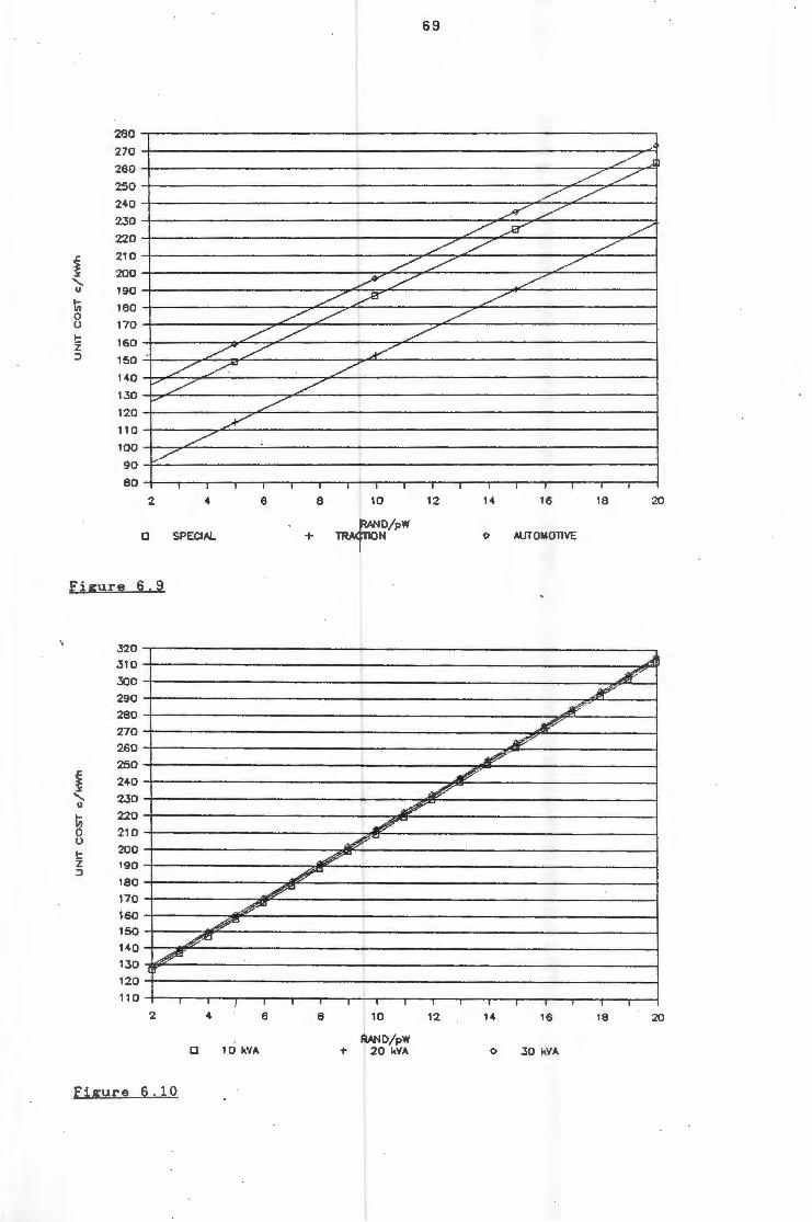
280
270
260
250
240
230
220
~ 210
~ 200
' u 190
lii 180 0 0 170 1- 160 z ::J 150
140
130
120
110
100
90
80
69
.// _;:
// I ,// I //
// / // //
/L_ / //
/~ //
// / //
/~ .--r/
/_ /
/ ~/
2 4 6
0 SPECIAL
/ /
/ I
I I I
8 10
RAND/pW + TRACTION
12
/ /
/
16 18 20
<> AUTOMOTIVE
Figure 6.9
320 310
300 290 280
270
260 250
~ 240 ~
' 230 u
tii 220
0 210 0
!:: 200 z ::J
190
180
170 160 150
140 130
120
110
I
~--flt!f?
/' /'
~~
~ ./" ~ ~
_LJ ~
df!P
2 .... 6 8
0 10 k'IA
10
RAND/pW ~ 20 kVA
12
A ...8{'/
f' ~-~ ~
# '
16 18 20
<> 30 kVA
Figure 6.10
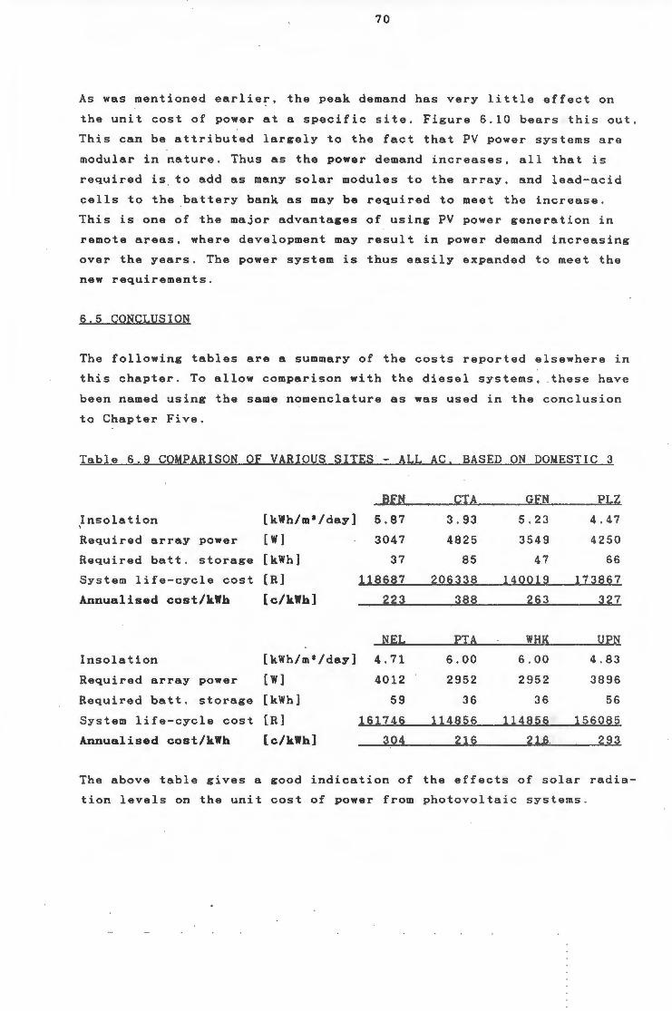
70
As was mentioned earlier, the peak demand has very little effect on
the unit cost of power at a specific site. Figure 6 . 10 bears this ou t.
This can be attributed largely to the fact that PV power systems are
modular in nature . Thus as the power demand increases , all that is
required is to add as many solar modules to the array, and lead-acid
cells to the battery bank as may be required to meet the increase .
This is one of the major advantages of using PV power generation i n
remote areas, where development may result in power demand increasing
over the years. The power system is thus easily expanded to meet the
new requirements.
6.5 CONCLUSION
The following tables are a summary of the costs reported elsewhere in
this chapter. To allow comparison with the diesel systems, these have
been named using the same nomenclature as was used in the conclusion
to Chapter Five.
Table 6.9 COMPARISON OF VARIOUS SITES - ALL AC. BASED ON DOMESTIC 3
Insolation ' Required array power
Required batt . storage
System life-cycle cost
Annualised cost/kWh
Insolation
Required array power
Required batt. storage
System life-cycle cost
Annualised cost/kWh
BFN CTA GFN PLZ
[kWh/ma/day] 5.87 3 . 93 5 . 23 4 . 4 7
[W] 3047 4825 3549 4250
(kWh] 37 85 47 66
[R] =1=1=8=6=8~7---=20~6~3~3~8~--1~4~0~0~1~9~~1~7~3~8~6~7
[c/kWh] ___ 2=2=3~----~3~8~8~----=2=6=3 ____ ~3~2~7
[kWh/ma/day]
[W]
[kWh]
[R]
[c/kWh]
NEL
4 . 71
4012
59
161746
304
PTA
6.00
2952
36
114856
216
WHK
6.00
2952
36
114856
216
UPN
4 . 83
3896
56
156085
293
The above table gives a good indication of the effects of solar radia
tion levels on the unit cost of power from photovoltaic systems .
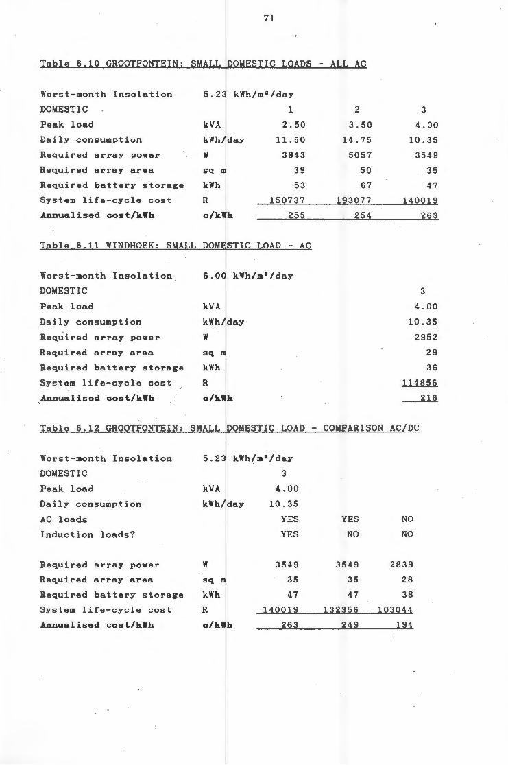
\
71
Table 6.10 GROOTFONTEIN: SMALL DOMESTIC LOADS - ALL AC
Worst-month Insolation
DOMESTIC
Peak load
Daily consumption
Required array power
Required array area
Required battery 'storage
System life-cycle cost
Annualised cost/kWh
5.23 kWh/m 2 /day
1
kVA
kWh/day
w sq m
kWh
R
c/kWh
2.50
11.50
3943
39
53
150737
255
Table 6.11 WINDHOEK: SMALL DOMESTIC LOAD - AC
Worst-month Insolation
DOMESTIC
Peak load
Daily consumption
Required array power
Required array area
Required battery storage
System life-cycle cost
Annualised cost/kWh
6.00 kWh/m 3 /day
kVA
kWh/day
w sq m
kWh
R
c/kWh
2
3.50
14.75
5057
50
67
193077
254
3
4 . 00
10.35
3549
35
47
140019
263
3
4.00
10.35
2952
29
36
114856
216
Table 6.12 GROOTFONTEIN: SMALL DOMESTIC LOAD -COMPARISON AC/DC
Worst-month Insolation
DOMESTIC
Peak load
Daily consumption
AC loads
Induction loads?
Required array power
Required array area
Required battery storage
System life-cycle cost
Annualised cost/kWh
5.23 kWh/m 2 /day
3
kVA 4.00
kWh/day
w sq m
kWh
R
c/kWh
10.35
YES
YES
3549
35
47
140019
263
YES
NO
3549
35
47
132356
249
NO
NO
2839
28
38
103044
194
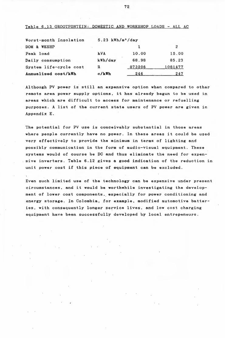
72
Table 6.13 GROOTFONTEIN: DOMESTIC AND WORKSHOP LOADS - ALL AC
Worst-month Insolation
DOM &. WKSHP
Peak load
Daily consumption
System life-cycle cost
Annualised cost/kWh
5.23 kWh/m 2 /day
1
kVA
kWh/day
R
c/kWh
10.00
68.98
873206
246
2
15 . 00
85 . 23
108147 7
247
Although PV power is still an expensive option when compared t o other
remote area power supply options, it has already begun to be used in
areas which are difficult to access for maintenance or refuel li ng
purposes. A list of the current state users of PV power are g i ven in
Appendix E.
The potential for PV use is conceivably substantial in those areas
where people currently have no power . In these areas it could be used
very effectively to provide the minimum in terms of lighting and
possibly communication in the form of audio-visual equipment. These
systems would of course be DC and thus eliminate the need for expen
sive inverters. Table 6.12 gives a good indication of the reduction in
unit power cost if this piece of equipment can be excluded.
Even such limited use of the technology can be expensive under present
circumstances, and it would be worthwhile investigating the develop
ment of lower cost components, especially for power conditioning and
energy storage. In Colombia, for example, modified automotive batter
ies, with consequently longer serv i ce l ives , and low c ost charging
equipment have been successfully deve l oped by loca l entrepeneurs.
77
unit volume. Wind power density, P, is defined as the power per unit
cross-sectional area of the windstream, and is given by:
P = 0,5 * p • u 1
Where:
p = density of the air
u = velocity of the windstream
From the above it can be seen that given the cube power dependency of
extractable wind power on wind speed, it is clearly the variability of
wind speed that is of importance in determining available wind power.
7.2.1 Climatological Effects on Wind Power
South Africa is located astride the subtropical high pressure belt
wh i ch is centred on average at 3QoS (Diab, 198Gb). The high pressure
systems in this belt do not give rise to much kinetic energy in the
atmosphere. To the south of 30°S, lies the westerly wind belt within
which oc9ur the travelling weather systems. These systems move from
west to east mainly along the coast, penetrating further into the in
terior in the winter than in the summer. Winds in these mid-latitudes
can be strong, particularly to the rear of a cyclone or cold front. I
7 . 2.2 Local Effects on Wind Power
In areas with apparently low wind power, certain topographical fea
tures can as much as double the wind speed, giving an eightfold in
crease in wind power. On the other hand, good wind potential can be
marred by the interference of topographical and other obstructions,
such as buildings and trees. In flat countryside, a fairly good esti
mate of the wind potential can be obtained by looking at the data from
the nearest weather station. However, if the countryside is hilly, it
is nearly impossible to estimate the available wind energy.
The large scale motion associated with the high and low pressure sys
tems provides the framework within which the smaller scale circula
tions occur. Solar heating and topographical features give rise to
local circulations which are generally light, but should by no means
be discounted as a source of energy. The Energy Research Institute is
currently investigating topographical effects in wind enhancement in
the Cape Agulhas region.
78
7.2.2 Wind Resource Surveys in South Africa
Evaluation of the data measured by the S.A. Weather Bureau at various
weather stations has been carried out (Diab, 1979). All indications
are that the coastal regions of the country generally experience the
highest wind speeds, but that there are also isolated pockets of
strong wind potential in the interior. This report is somewhat mis
leading in its findings, as it was reliant on very few recording
stations, with a poor spatial distribution over the country .
A more detailed regional study carried out over KwaZulu and Natal
(Diab, 1986a), making use of data other than that purely obtainable
from recording stations, has revealed greater potential than was first
thought. It is also apparent from the widespread use of windpumps
throughout the country that there is definitely a greater potential
for wind power generation than published surveys would lead one to
believe. However, the assessment of the true potential of the wind
resource would necessitate more detailed measurement. This monitoring
would be guided by the existing baseline data, and a thorough study of
the local features which could enhance prevailing wind speeds in a
particular region.
To assess the wind energy potential some experts recommend measuring
the wind resource at a potential site for five years, while others
feel that three years will be sufficient. The degree of accuracy
required is a function of the investment being made i.e. a 50% error
in estimation will have far greater implications if a 100 kW machine
to supply a small town is being installed as compared to a 1 kW
machine to supply power for a holiday home.
It should be borne in mind, however, that records taken over short
periods e.g. a year can be off ± 30% from long-term averages. For this
reason measurements should be compared with data from the nearest
weather station. By comparing in this way it is possible to increase
the degree of confidence in data collected over a short period. How
ever, the less that is known about the actual wind conditions at a
site, the more that is left to chance when installing a system .
Nielsen (1978) is a good guide to wind power estimation techniques ,
while Diab (1986a) has documented some useful biological indicators
which can be used to determine local wind resource potential.
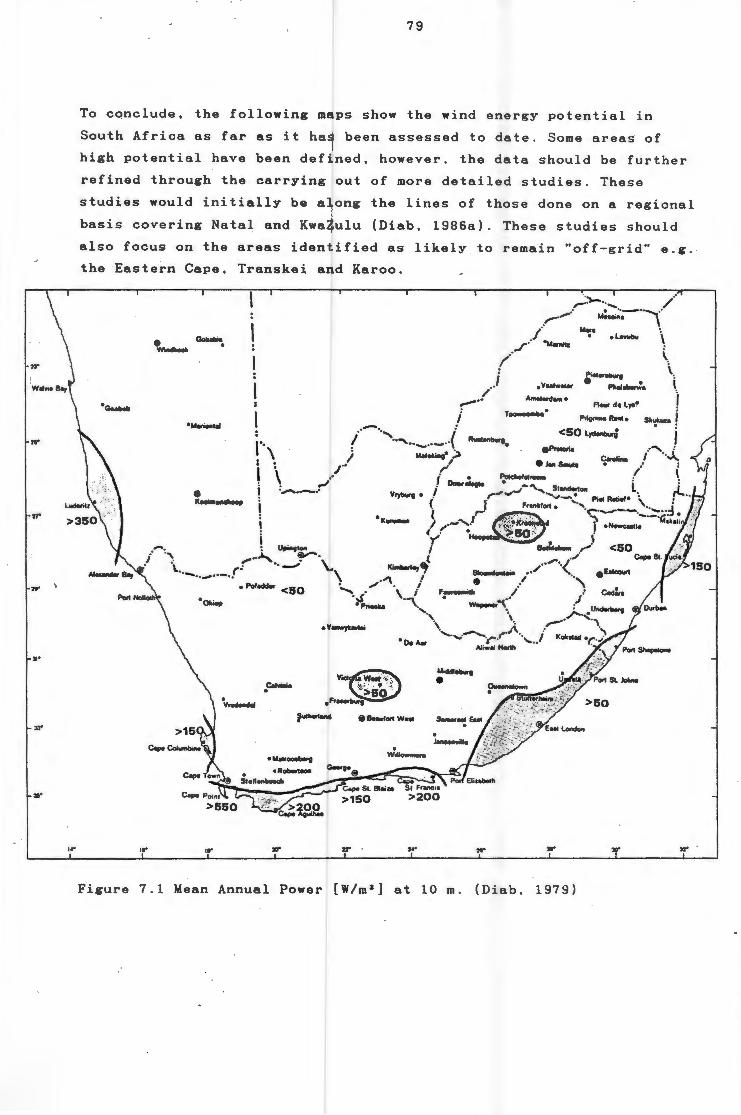
os•
,.
...
...
79
To conclude, the following maps show the wind energy potential in
South Africa as far as it has been assessed to date. Some areas of
high potential have been defined, however, the data should be further
refined through the carrying out of more detailed studies. These
studies would initially be along the lines of those done on a regional
basis covering Natal and KwaZulu (Diab, 1986a). These studies should
also focus on the areas identified as likely to remain "off-grid" e.g.
the Eastern Cape, Transkei and Karoo.
... . ..
l
'
.v....,u...;
8BuulonW••
.,. . .. . Figure 7.1 Mean Annual Power [W/m 2 ] at 10m. (Diab, 1979)
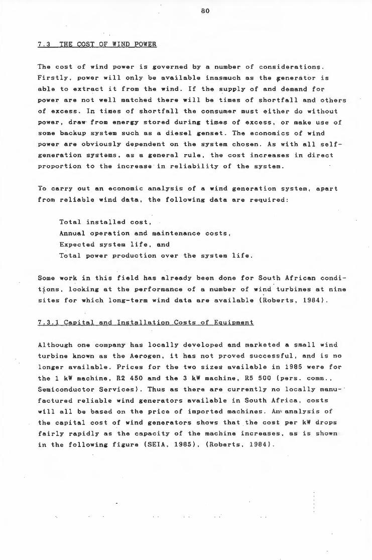
80
7.3 THE COST OF WIND POWER
The cost of wind power is governed by a number of considerations .
Firstly, power will only be available inasmuch as the 'ener~t6r is
able to extract it from the wind. If the supply of and demand for
power are not well matched there will be times of shortfall and others
of excess. In times of shortfall the consumer must either do without
power, draw· from energy stored during times of excess , or make use of
some backup system such as a diesel genset . The economics of wind
power are obviously dependent on the system chosen. As with all self
generation systems, as a general rule, the cost increases in direct
proportion to the increase in reliability of the system .
To carry out an economic analysis of a wind generation system, apart
from reliable wind data, the following data are required:
Total installed cost,
Annual operation and maintenance costs,
Expected system life, and
Total power production over the system life.
Some work in this field has already been done for South African condi
t~ons, looking at the performance of a number of wind turbines at nine
sites for which long-term wind data are available (Roberts, 1984).
7.3 . 1 Capital and Installation Costs of Eguipment
Although one company has locally developed and marketed a small wind
turbine known as the Aerogen, it has not proved successful, and is no
longer available. Prices for the two sizes available in 1985 were for
the 1 kW machine, R2 450 and the 3 kW machine, R5 500 (pers. comm.,
Semiconductor Services). Thus as there are currently no locally manu- ·
factured reliable wind generators available in South Africa, costs
will all be based on the price of imported machines. An analysis of
the capital cost of wind generators shows that the cost per kW drops
fairly rapidly as the capacity of the machine increases, as is shown
in the following figure (SEIA, 1985), (Roberts, 1984) .
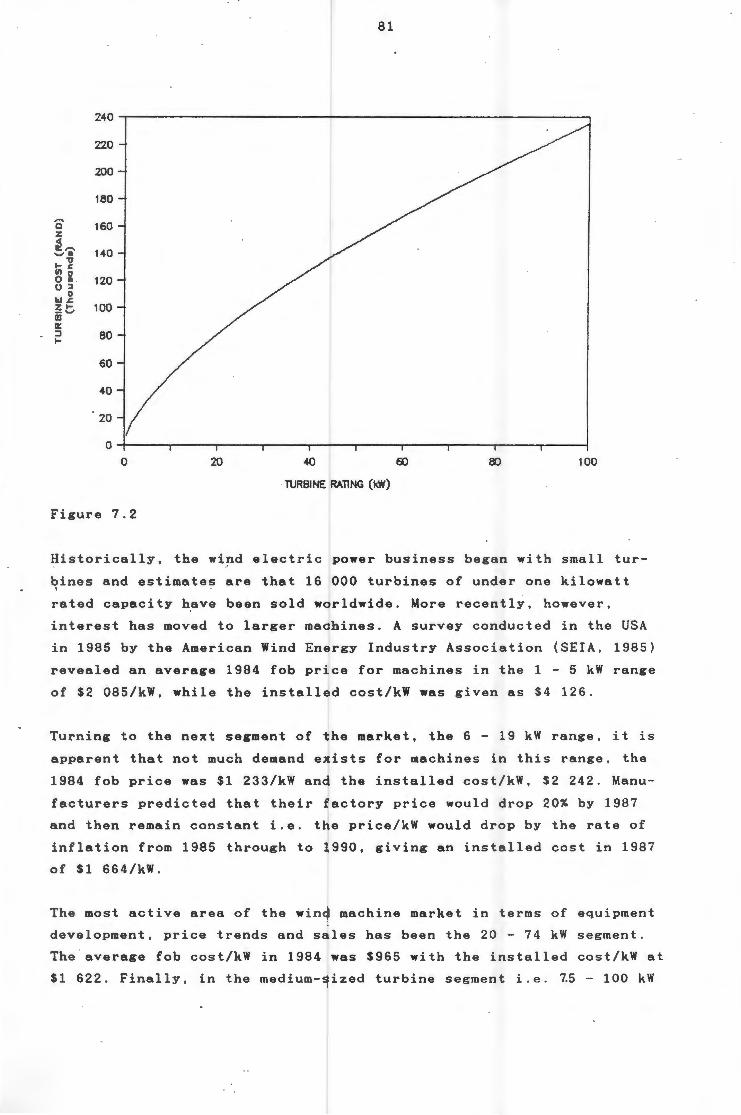
81
240
220
200
180
,.... 0 160 z
~'"' 140 ~tl
1-'¥ (/) 0 0 tl 120 0 ::l
0 WJ:. Zl-- '-J
100 m a: :::l 80 1-
60
40
20
0 0 20 40 60 80 100
TURBINE RATING (kW)
Figure 7.2
Historically, the wipd electric power business began with small tur
bines and estimates are that 16 000 turbines of under one kilowatt . rated capacity h.ave been sold worldwide. More recently, however,
interest has moved to larger machines. A survey conducted in the USA
in 1985 by the American Wind Energy Industry Association (SEIA, 1985)
revealed an average 1984 fob price for machines in the 1 - 5 kW range
of $2 085/kW, while the installed cost/kW was given as $4 126.
Turning to the next segment of the market, the 6 - 19 kW range, it is
apparent that not much demand exists for machines in this range, the
1984 fob price was $1 233/kW and the installed cost/kW, $2 242. Manu
facturers predicted that their factory price would drop 20% by 1987
and then remain constant i.e. the price/kW would drop by the rate of
inflation from 1985 through to 1990, giving an installed cost in 1987
of $1 664/kW.
The most active area of the wind machine market in terms of equipment
development, price trends and sales has been the 20 - 74 kW segment.
The average fob cost/kW in 1984 was $965 with the installed cost/kW at
$1 622. Finally, in the medium-sized turbine segment i.e . ~5 - 100 kW
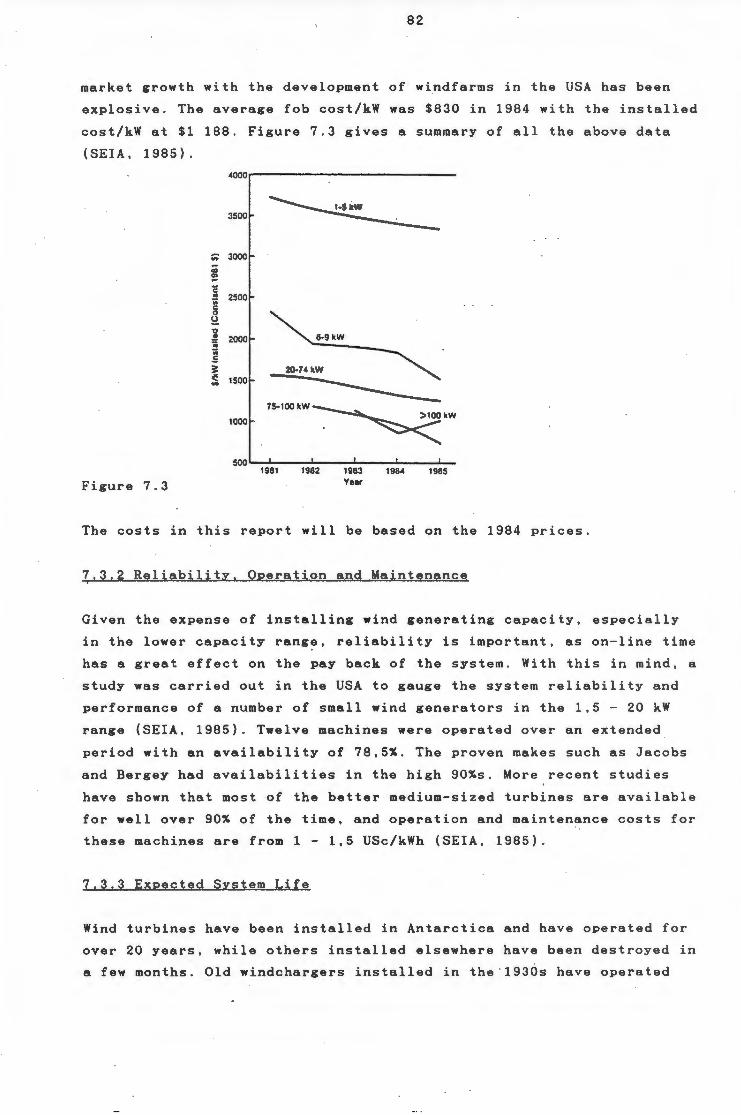
82
market growth with the development of windfarms in the USA has been
explosive. The average fob cost/kW was $830 in 1984 with the installed
cost/kW at $1 188. Figure 7 . 3 gives a summary of all the above data
(SEIA, 1985).
~000
3500
;; ; ~ c .. Vi c 0
~ .., ~ 6-9kW
~ .: 3 20-7~ kW <~:! 1500 ..
1000 75-100kW~ >~
. ~kW
500'-~--~--~--~--...1..-1981 1982 1983 198<4 1985
Figure 7.3 Year
The costs in this report will be based on the 1984 prices.
7.3 . 2 Reliability, Operation and Maintenance
Given the expense of installing wind generating capacity, especially
in the lower capacity range, reliability is important, as on-line time
has a great effect on the pay back of the system. With this in mind, a
study was carried out in the USA to gauge the system reliability and
performance of a number of small wind generators in the 1,5 - 20 kW
range (SEIA, 1985). Twelve machines were operated over an extended
period with an availability of 78,5%. The proven makes such as Jacobs
and Bergey had availabilities in the high 90%s. More recent studies
have shown that most of the better medium-sized turbines are available
for well over 90% of the time, and operation and maintenance costs for
these machines are from 1- 1,5 USc/kWh (SEIA, 1985).
7 . 3.3 Expected System Life
Wind turbines have been installed in Antarctica and have operated for
over 20 years, while others installed elsewhere have been destroyed in
a few months . Old windchargers installed in the . 1930s have operated
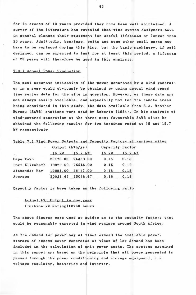
83
for in excess of 40 years provided they have been well maintained. A
survey of the literature has revealed that wind system designers have
in general planned their equipment for useful lifetimes of longer than
20 years. Admittedly, bearings, belts and some other small parts may
have to be replaced during this time, but the basic machinery, if well
designed, can be expected to last for at least this period. A lifespan
of 25 years will therefore be used in this analysis.
7.3.4 Annual Power Production
The most accurate indication of the ·power generated by a wind generat
or in a year would obviously be obtained by using actual wind speed
time series data for the site in question. However, as these data are
not always easily available, and especially not for the remote areas
being considered in this study, the data available from S.A . Weather
Bureau (SAWB) stations were used by Roberts (1984). In his analysis of
wind-powered generation at the three most favourable SAWB sites he
obtained the following results for two turbines rated at 15 and 15,7
kW respectively:
Table 7.1 Wind Power Outputs and Capacity Factors at various sites
Output (kWh/yr) Capacity Factor
15 kW 15.7 kW 15 kW 15 . 7 kW
Cape Town 20176.00 24458.00 0.15 0.18
Port Elizabeth 19920.00 25545.00 0.15 0.19
Alexander Bay 19984.00 25137.00 0.18 0 . 18
Average 20026.67 25046 . 67 0.16 0.18
Capacity factor is here taken as the following ratio:
Actual kWh Output in one year
(Turbine kW Rating)*8760 hours
The above figures were used as guides as to the capacity factors that
could be reasonably expected in wind regimes around South Africa.
As the demand for power may at times exceed the available power,
storage of excess power generated at times of low demand has been
included in the calculation of unit power costs. The systems examined
in this report are based on the principle that all power generated is
passed through the power conditioning and storage equipment, i.e.
voltage regulator 1 batteries and inverter.
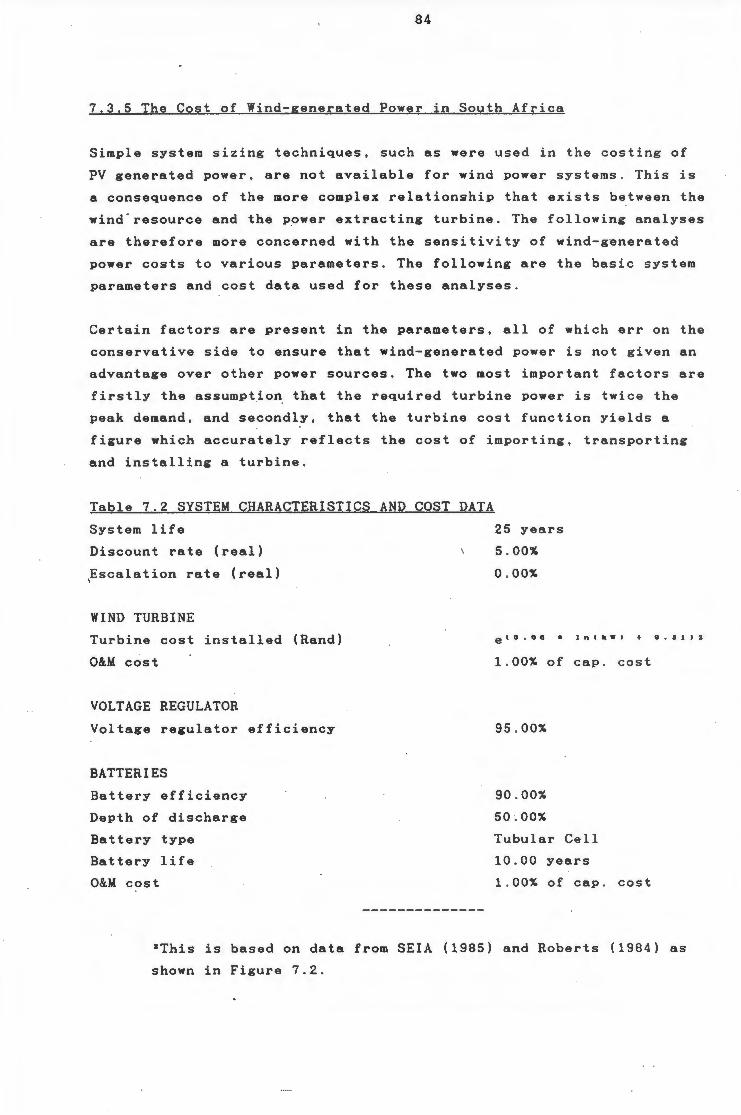
84
7.3.5 The Cost of Wind-generated Power in South Africa
Simple system sizing techniques, such as were used in the costing of
PV generated power, are not available for wind power systems . This is
a consequence of the more complex relationship that exists between the
wind-resource and the power extracting turbine. The following analyses
are therefore more concerned with the sensitivity of wind-generated
power costs to various parameters. The following are the basic system
parameters and cost data used for these analyses .
Certain factors are present in the parameters, all of which err on the
conservative side to ensure that wind-generated power is not given an
advantage over other power sources. The two most important factors are
firstly the assumption that the required turbine power is twice the
peak demand, and secondly, that the turbine cost function yields a
figure which accurately reflects the cost of importing , transporting
and installing a turbine.
Table 7.2 SYSTEM CHARACTERISTICS AND COST DATA
System life 25 years
Discount rate (real)
~scalation rate (real)
WIND TURBINE
Turbine cost installed (Rand)
O&M cost
VOLTAGE REGULATOR
Voltage regulator efficiency
BATTERIES
Battery efficiency
Depth of discharge
Battery type
Battery life
O&M cost
5.00%
0 . 00%
e<0 . 80 * lnCkWJ + 11.31)2
1 . 00% of cap. cost
95 . 00%
90 . 00%
50.00%
Tubular Cell
10.00 years
1 . 00% of cap . cost
3 This is based on data from SEIA (1985) and Roberts (1984) as
shown in Figure 7.2.
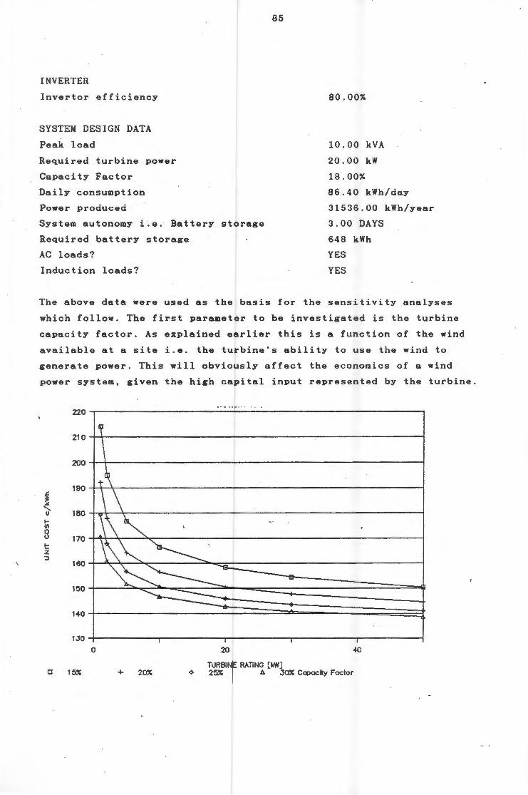
INVERTER
Invertor efficiency
SYSTEM DESIGN DATA
Peak load
Required turbine power
Capacity Factor
Daily consumption
Power produced
System autonomy i.e. Battery storage
Required battery storage
AC loads?
Induction loads?
85
80.00%
10.00 kVA
20.00 kW
18.00%
86.40 kWh/day
31536.00 kWh/year
3.00 DAYS
648 kWh
YES
YES
The above data were used as the basis for the sensitivity analyses
which follow. The first parameter to be investigated is the turbine
capacity factor. As explained earlier this is a function of the wind
available at a site i.e. the turbine's ability to use the wind to
generate power. This will obviously affect the economics of a wind
power system, given the high capital input represented by the turbine.
220
210
200
190 .c 3: .X
' 180 IJ
1-Ill 0 0 170 1-z ::>
160
150
140
1JO 0 20 40
TURBINE RATiNG [kW] a 15~ + 2~ ~ 25~ 6. J~ C~ity Foetor
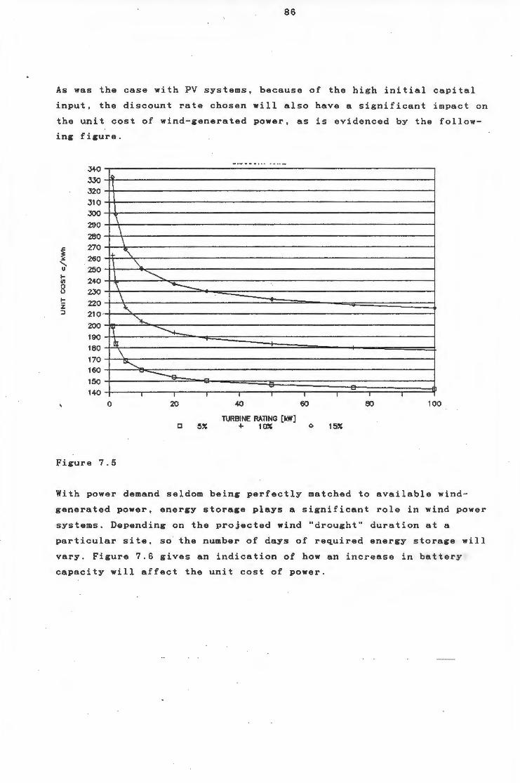
86
As was the case with PV systems, because of the high initial capital
input, the discount rate chosen will also have a significant impact on
the unit cost of wind-generated power, as is evidenced by the follow
ing figure.
340 JJO 320 310 300 290 280
~ 270 260
' u 250 1-
240 rn 0 0 2.30 '= 220 z :l 210
200 190 180 170 160 150
\ \ \
I+ " \. \ "'--.... \ ....___ \
' .~ 11 ~ Bl \
""-.,_
~
140 I I
0 20 40 60 80 100
lURBINE RATING [kW] c 5X + 1 OX <> 1 5X
Figure 7 . 5
With power demand seldom being perfectly matched to available wind
generated power, energy storage plays a significant role in wind power
systems. Depending on the projected wind "drought" duration at a
particular site, so the number of days of required energy storage will
vary. Figure 7.6 gives an indication of how an increase in battery
capacity will affect the unit cost of power.
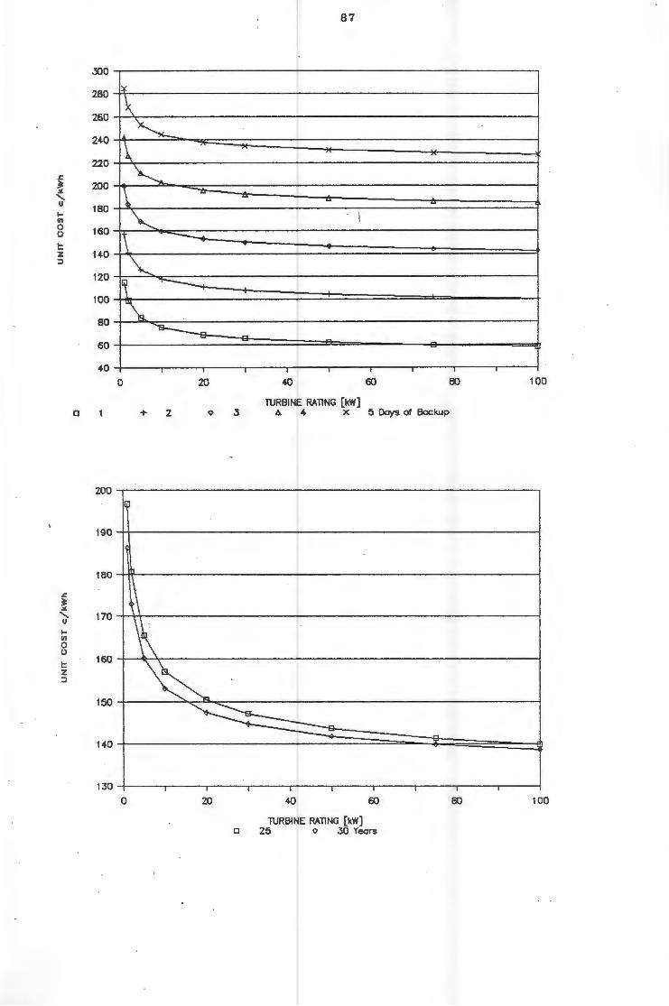
87
.300
280
260
240
220 ~
3: 200 .:11.
' u 180 1-en 0 160 0
t: z 140 :::J
120
100
80
be
\ ~
\ ~
i\ ~
"'- i
1\ -----...
~ I'
.,.._____
~ ~-=
60
40 0 20 40 60 80 100
TURBINE RATING (kW] 0 + 2 A 4 X 5 Days of Bockup
200
190
180
.c 3: .:11.
' 170 u 1-en 0 0
t: 160 \\ z :::J
150
140
130 0 20 40 60 80 100
TURBINE RATING (kW) o 25 o .:SO Years
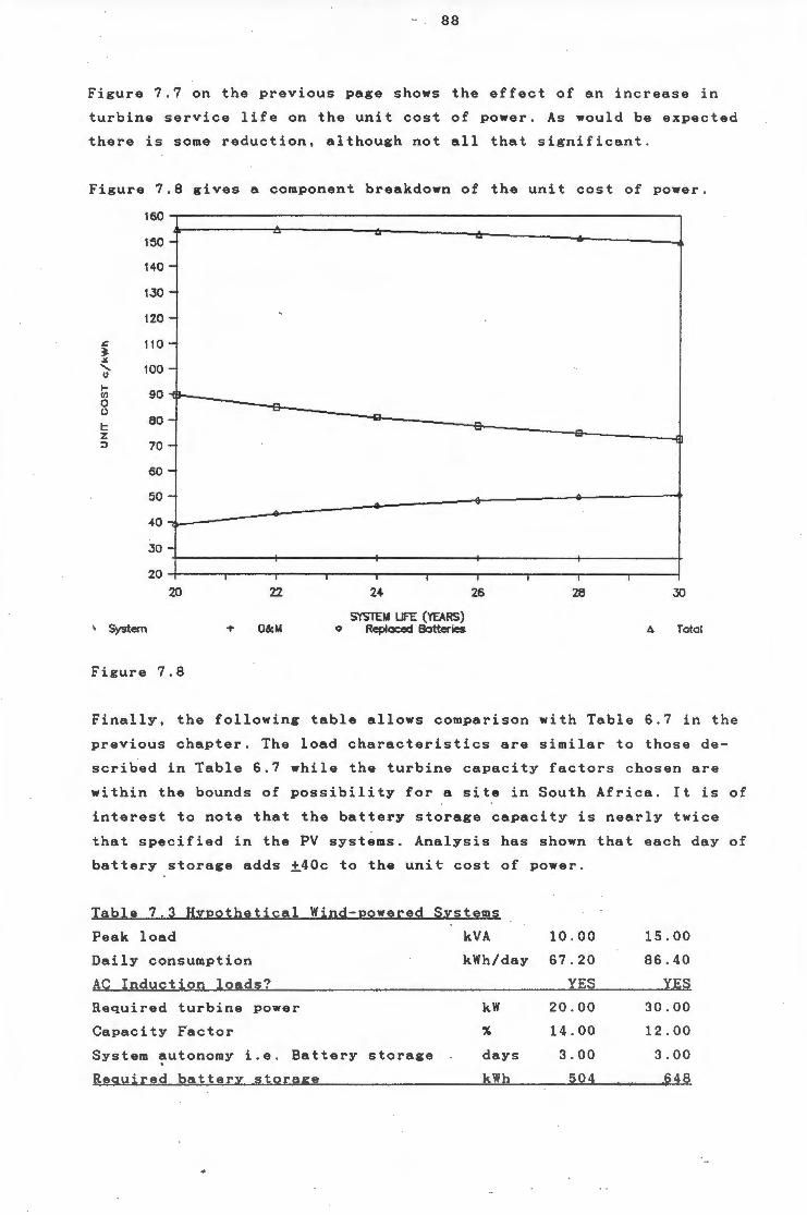
88
Figure 7.7 on the previous page shows the effect of an increase in
turbine service life on the unit cost of power. As would be expected
there is some reduction, although not all that significant.
Figure 7.8 gives a component breakdown of the unit cost of power .
160
-150 -140 -1.30 -120 - '
s: 110 ~
-"' '- 100 0 -._
90 (/) -f 0 0
t 80 -z :J 70 -
60 -50 -40
JO -20
20 22 24 26 28
SYSTEI!I UFE (YEARS) ' System + 0&111 <> Replaced Botteries 6. Total
Figure 7.8
Finally, the following table allows comparison with Table 6.7 in the
previous chapter. The load characteristics are similar to those de
scribed in Table 6.7 while the turbine capacity factors chosen are
within the bounds of possibility for a site in South Africa. It is of
interest to note that the battery storage capacity is nearly twice
that specified in the PV systems. Analysis has shown that each day of
battery storage adds ~40c to the unit cost of power.
Table 7.3 H;yEothetical Wind-Eowered S;ystems
Peak load kVA 10.00 15.00
Daily consumption kWh/day 67.20 86 . 40
AC Induction loads? YES YES
Required turbine power kW 20 . 00 30.00
Capacity Factor % 14.00 12.00
System ~utonomy i.e . Battery storage days 3.00 3 . 00
Reguired batter;y storage kWh 504 648
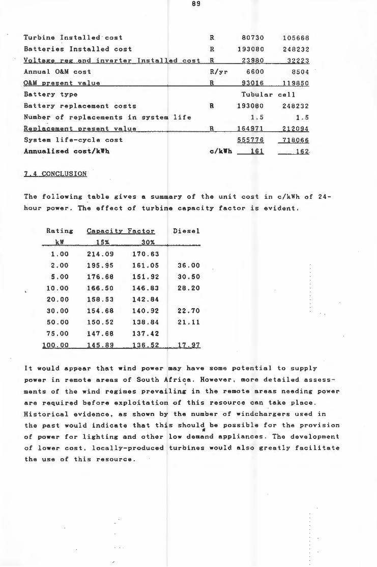
Turbine Installed cost
Batteries Installed cost
89
R
R
Voltage reg and inverter Installed cost R
Annual O&.M cost
O&M present value
Battery type
Battery replacement costs
Number of replacements in system life
Replacement present value
System life-cycle cost
Annualised cost/kWh
7 .4 CONCLUSION
R/yr
R
R
R
c/kWh
80730
193080
23980
6600
93016
105668
248232
32223
8504
119850
Tubular cell
193080
1.5
164971
555776
161
248232
1.5
212094
718066
162
The following table gives a summary of the unit cost in c/kWh of 24-
hour power. The effect of turbine capacity factor is evident.
Rating Capacit;z:: Factor Diesel
kW 15% 30%
1.00 214.09 170.63
2.00 195.95 161.05 36.00
5 . 00 176.68 151.92 30.50
10.00 166.50 146.83 28.20
20.00 158.53 142.84
30.00 154.68 140.92 22.70
50.00 150.52 138.84 21.11
75.00 147.68 137.42
100.00 145.89 136.52 17.97
It would appear that wind power may have some potential to supply
power in remote areas of South Africa. However, more detailed assess
ments of the wind regimes prevailing in the remote areas needing power
are required before exploitation of this resource can take place.
Historical evidence, as shown by the number of windchargers used in
the past would indicate that this should be possible for the provision
" of power for lighting and other low demand appliances. The development
of lower cost, locally-produced turbines would also greatly facilitate
the use of this resource.

90
CHAPTER EIGHT
SMALL SCALE HYDROELECTRIC POWER
The climate of Southern Africa is characterised by a steep c limatic
gradient from the generally wetter eastern coast to the semi - ar i d and
desert regions of the west·. The variability of annual rainfall i n both
time and space increases with increasing aridity. Surface runof f per
unit area also falls with increase in aridity due to the combined
effects of lowered volume and raised rainfall variability, plus i n
creases in evaporation from land surfaces and vegetation . Typically ,
river flows vary over a wide range from year to year.
Evaporation losses from stored water are high. The water levels and
corresponding surface areas and shorelines of storage reservoirs
fluctuate over a wide range, in response to variations in inflow ,
while the flow regimes of rivers downstream are radically altered, and
become dependent on the operating criteria of the impoundments .
In the light of the above, the potential for widespread large-scale
use of hydropower in South Africa is obviously limited. However, there
are a number of areas and way~ in which it could be put to use, to
meet the needs of small consumers.
8.1 HYDROPOWER SCHEME CONFIGURATIONS AND TECHNOLOGY
This section gives a brief overview of the various ways i n wh ich
hydropower schemes can be implemented, especially on a small s c ale.
8.1.1 Run of River Schemes
Run of river (ROR) schemes make use of the river's flow to drive a
water wheel or turbine as it passes, and do not have any significant
reservoir, at the most a small head pond providing daily storage. They
are of particular interest in the provision of power in remote areas,
and have been used extensively in remote areas of China , Nepal, the
Phillipines, Papua New Guinea, Indonesia, Colombia and Peru .

91
If used to drive a generator to provide electrical power to a varying
load throughout the day, a true ROR scheme is impractical on all South
African rivers, with the exception possibly of irrigation schemes such
as the Fish River below the outlet of the Orange-Fish tunnel. In all
other cases some form of dam or diversion weir is required to impound
the water which can be drawn down during the day, and replenished
during the night. Of course it would be preferrable to size such a dam
to provide seasonal storage, based on mean river flows and water
requirements for power generation.
Even with seasonal storage, when rainfall falls below the mean aver
age, the power plant will obviously be unable to meet the demands made
upon it. Thus, unless the scheme is interconnected electrically with
another supply with excess generating capacity, it will be necessary
to provide some source of "firming" generation capacity from another
source, i.e. a hybrid configuration would be needed. This firming
capacity would typically be provided by a diesel genset, or possibly
some other reliable renewable power source. Provision of this firming
power could represent a significant expense. It is therefore important
that the sizing of the dam be based on as accurate river flow data as
possible.
ROR schemes with impoundments often lend themselves to extension, as
and when the demand requires it. This is achieved by cascading the
tailwater from one turbine to the inlet of the next. The original
storage dam then serves a number of stations and the amortisation of
the capital cost of the civil works is spread over them. This is
naturally subject to there being sufficient gradient in the river's
course. One feature of a cascading scheme is its inherent capacity to
meet peak loads. At times excess water will be trapped between the
stations, either in the stream bed or canals, thus allowing lower
stations to generate more electricity than under constant flow condi
tions through all stations. This capability can be enhanced through
the addition of intermediate small volume reservoirs .
The above installations would typically be in the kilowatt range i.e.
from 2 kW upwards. Another demand range however exists in remote areas
of this country, where power consumptions in the watt range exist.
Power at this level is required for lighting and the operation of a
number of small appliances such as clinic refrigerators, audio-visual
equipment for education and recreation. This power cou~d easily be
92
supplied in many areas with the harnessing of a small stream, or the
flow through a domestic water reticulation system . Such small systems
have been designed and produced i~ Colombia . These make use of a
Pelton wheel, a modified automotive alternator and batteries. The
batteries are based on standard automotive battery components with a
few modifications to ensure longer life and deeper cycle charge and I
discharge characteristics.
8.1.2 Multi-purpose Schemes
In these schemes, the generation of electricity may not be the prime
consideration, and is sometimes more in the nature of a by-product .
Their prime purpose is usually to provide some form of equalisation of
the flow in a basin, by storing water during the times of high rain
fall to allow for its use during the dry periods. Storage capacity is
often sufficient to provide for needs in statistically anticipated low
rainfall years.
The Orange River scheme is an example of a large-scale multi-purpose
scheme, although the amount of electrical energy being produced by the
scheme is relatively small. However, because the release of the water
to lower riparian users does not have to take place at specific times
~f the day, it can be released at times to coincide with peak demands
on the grid, · and thus provide low-cost peak power. The Kouga river
irrigation scheme also makes use of some of the water flow for genera
tion of power for use in the Gamtoos valley (Langford and Webb, 1970).
The Ox-bow scheme in Lesotho will similarly make use of HEP generation
to dissipate the potential energy in the water being released to lower
levels.
Extensive irrigation development of South African rivers has already
taken place, but little effort has been m~de ~o combine these develop
ments with the generation of power. This has resulted from the appa
rent lack of coordination between Eskom and the Department of Water
Affairs. In addition, the Electricity Act requires that Eskom should
generate and transmit power at the lowest possible cost. In the case
of straight hydro-electric power (HEP) generation , the cost of power
generation is higher than that from the eqivalent thermal power sta
tion, primarily because of the high civil works cos t component . How
ever, if a multi-purpose scheme were to be developed, very little, if
any of the civil costs would be borne by the electricity generation
93
component of the scheme. There is also great potential for the use of
small ROR schemes which could be installed in the many kilometres of
ir r igation canals that cross parts of South Africa .
In a study carried out in Australia, a total of 1 248 GWh/yr was iden
t if ied as being potentially available at existing irrigation and water
supply dams (Water Power and Dam Construction, 1987) . This study only
looked at plant betwen 100 kW and 20 MW, and revealed an estimated
cost/kW installed of $620 and $2 860, and the cost/kWh from 0,7 to 5,6
cents . There is no doubt a great deal of potential for installations
of smaller capacity.
Re l ated to multi-purpose development of water storage facilities . is a
development by a US company of the PowerBarge (Broome, 1986). This
prefabricated unit is aimed at use on medium-sized rivers with an
annual flow of from 28 - 280 m3 /sec that can be controlled by dams as
low as 3,2 m. The unit consists of a fully floating hydroelectric
station supported by two barges, one above and the other below the
dam. The estimated total capital cost of an installation is estimated
to be 20 - 30% lower than that for a conventional system at the same
s ite.
8 .1. 3 REP Eguipment Selection Criteria
The purpose of this section is to present some criteria for the
installer to select equipment for micro hydro plants of up to about
150 kVA. The context is the application of micro scale hydropower for
remote rural communities for productive activities (grain milling,
workshops, food processing, sawmills, and so on). A brief survey of
the criteria used in selecting equipment for micro hydro plants for
developing country applications has shown, as would be intuitively
expected, that cost and simplicity of operation are critical factors.
In the rural, developing scenario capital cost is generally a severe
constraint, and reliability, maintainability and simplicity of opera
tion are paramount. Plant efficiency is important, but within the con
straints of what is achievable with the resources a¥ailable . For
example , locally made turbines used in many countries _achieve effi
ciencies in the range of 70 to 80 %. Improving the efficiency through
h i gher cost manufacturing techniques or more elaborate designs is sub
ject to the law of limiting returns.
94
The capital cost of the installation has to be kept to a level such
that the final energy costs are comparable with (and preferably lower
than) the immediate alternatives. These will normally be extension of
the grid or provision of a diesel generator.
The Intermediate Technology Development Group (ITDG) has been running
a series of demonstration micro hydro projects in Nepal, Sri Lanka,
Colombia and Peru. These schemes have involved the use of locally made
turbines (in some cases after initially using British ones). The ob
jective is to provide power for small processing industries, with a
probable additional benefit of providing some domestic electric power .
These plants generally aim for load factors of 25 - 40%. Even with
these high (for small plants) load factors, there . is a severe con
straint on the capital cost that can be justified. A typical target
cost breakdown would be:
Penstock
Other civil work
Mechanical and electrical equipment
Engineering supervision
30 % of total
20 %
40 %
10 %
~f the target total system cost of US$1000 - US$2000/kVA. $400 - $800
would be for the mechanical and electrical components (not including
electrical transmission/distribution). These costs, it should be
emphasised, are not unrealistic. There are plenty of examples of
reliable and well built micro hydro plants constructed to these cost
targets using locally made turbines of acceptable reliability.
Penstock Pipes
There is a wide choice of pipes available, the relative prices of
which vary considerably. As mentioned before, pipe costs can made up a
third of the total installation cost so it is certainly worth compar
ing all available possibilities. Handling costs should also be consid
ered. For example, GRP pipe may well be preferable to cheaper ductile
iron when the costs of transport to a remote site with difficult
access are taken into consideration. · In other instances , PVC pipe may
be suitable, or steel pipe welded on site .
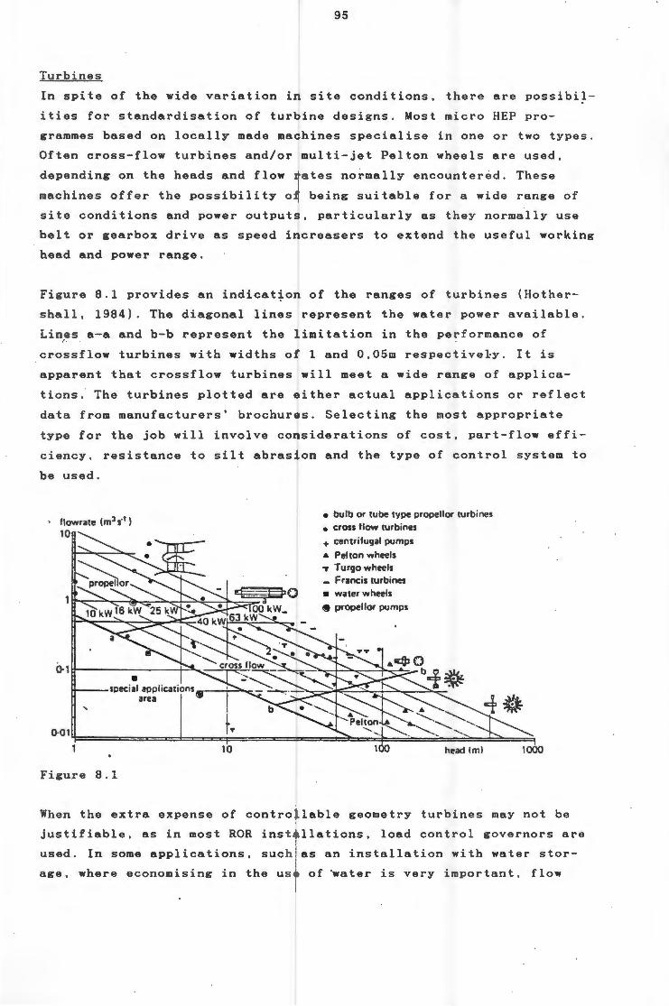
95
Turbines
In spite of the wide variation in site conditions, there are possibi~
it i es for standardisation of turbine designs . Most micro HEP pro
grammes based on locally made machines specialise in one or two types .
Often cross-flow turbines and/or multi-jet Pelton wheels are used,
depending on the heads and flow rates normally encountered. These
machines offer the possibility of being suitable for a wide range of
site conditions and power outputs, particularly as they normally use
belt or gearbox drive as speed increasers to extend the useful working
head and power range .
Figure 8.1 provides an indicat~on of the ranges of turbines (Hother
shall, 1984). The diagonal lines represent the water power available.
Lines a-a and b-b represent the limitation in the performance of r
crossflow turbines with widths of 1 and 0,05m respectively. It is
apparent that crossflow turbines will meet a wide range of applica
tions. The turbines plotted are either actual applications or reflect
data from manufacturers' brochures. Selecting the most appropriate
type for the job will involve considerations of cost, part-flow effi
ciency, resistance to silt abrasion and the type of control system to
be used.
' flowrate (m3 s·1 )
10
• 1+---special applications_--+..:::O..oc:
area
'
10
Figure 8.1
• bulb or tube type propeller turbines • cross flow turbines ~ centrifugal pumps • Pelton wheels "T Turgo wheels - Francis turbines • water wheels 8 propeller pumps
When the extra expense of controllable geometry turbines may not be
justifiable, as in most ROR installations, load control governors are
used . In some applications, such as an installation with water stor
age, where economising in the use of ~ater is very important, flow
96
control governing may be preferable. I~ most installations, however,
it is not necessary except perhaps for a manual change in guide vane
position or blade angel, to cope with day to day flow variations . The
part-flow efficiency can be important when the available flow at a
site is predicted to fall below the rated flow for a significant por
tion of the year. Mixed flow pumps operating as turbines have low cost
but poor part-flow characteristics. Nonetheless they certainly merit
consideration in cases where full flow conditions can be guaranteed ,
although that is not common.
Materials and construction techniques for turbine manufacture have
changed in recent years. New materials, such as plastic for runners ,
are being used by some manufacturers for very small turbines. Oil
lubricated journal and Michel thrust bearings used on larger machines
are not generally used for micro hydro, and spherical roller bearing
are common for impulse turbines. Water lubricated cutlass type bear
ings are used for some very small propeller turbines. Regular e.g.
annual bearing changes are simple and inexpensive .
Finally, it should be borne in mind that many micro scale applications
can be adequately supplied using a centrifugal pump run in reverse.
These have been used with great success in Colombia, South America, to
~barge batteries for lighting and television. Locally, engineers at
the Dept of Agricultural Engineering in Pretoria have investigated
their potential, as have students at the Universities of Natal and
Cape Town.
REP Generators and their control
On isolated micro hydro plants, synchronous generators have to be
used, normally of the type mass-produced for diesel generator sets
(generally four pole, 1500 or 1800 rev/min). Lower speed multi-pole
machines of this size are generally very expensive (at least twice the
price for 100 rev/min). Induction generators used for paralleling with
the grid have the disadvantage in most developing country applications
of not allowing isolated operation. Also the capacitors that normally
have to 6e fitted to compensate for the reactive current drawn from
the grid can be expensive. It is possible to run induction generators
independently, but voltage control is required so that the excitation
provided by capacitance across the terminals can be varied with load
and phase angle. Such a controller is at present under development in
the UK, co-sponsored by ITDG and the Science and Engineering Research
Council.

97
Voltage control of synchronous generators can be by electronic or
static automatic voltage regulators (AVR). Electronic AVRs have been
found to be the most unreliable part of micro hydro systems , and it is
recommended that static voltage regulators be used wherever possible,
although it does seem that electronic AVRs are at last becoming more
reliable. Overspeed rating · of generators is an important constraint .
The mass-produced synchronous generators are not normally rated for
the overspeed they may experience when used for micro hydro and manu
facturers must normally strengthen the rotors to meet the overspeed
specification.
The protection equipment normally required includes an over-current
device to trip the circuit breaker, over-voltage trip to cut the field
in the event of overspeed and under- and over- frequency trips are
generally used to operate the circuit breaker. It is also normally
necessary to fit a means of shutting down the turbine automatically in
the event of overspeed, since prolonged running at overspeed is likely
to cause damage.
If electronic load controllers are fitted, the ballast load should be
connected directly to the alternator, protected only by fuses . The
ma i n load should be fed by circuit breaker with auxiliary contacts for
tripping from the protection devices mentioned above.
HEP System Control
Automatic and remote control techniques can be put to good use on
micro hydro plants. Examples are : remote monitoring and control of the
plant; automatic start up and shut down governed by s~orage water
level; and, load management by automatic switching on or off of load
according to predetermined priorities. Automatic control of sluice
gates, penstock valves, trashracks, and so on, may also be worth
consideration.
It is important to remember that micro hydro plants remain exposed to
all sorts of potential natural calamitie~. and automation is no sub
stitut~ for personal monitoring . Control equipment can also be diffi
cu l t for semi-skilled artisans to repair. Care also has to be taken
not to decrease the system reliability by building in too many extra
failure modes . Electronic load control governors for speed regulation
are now widely used and generally considered the most appropriate form
of speed control for micro hydro plant . Their main advantages are:
98
1. Price
2. Reliability
3. Speed of response
4. No fly wheel required, and
5. Simplification of the turbine design.
Phase angle control electronic load governors, which use a single
resistive load able to absorb the full output of the generator have
been used by ITDG and have been found to be very satisfactory. Poten
tial disadvantages of wave form distortion and radio interference do
not, in practice, prove to be real problems. The basic principle of
operation is to sense the frequency, and the power fed to the ballast
load is then varied to adjust the total load, thus keeping the speed
constant. Use of multiple ballast loads and zero voltage switching of
increments of ballast is an alternative approach, but is generally
more complex.
~he use of mechanical/hydraulic or electro-mechanical governors is
more appropriate on larger systems and on plants where water economiz
ing is important. A combination of slow response flow governing with
electronic load control can also be used for water economising.
8.2 HYDROPOWER POTENTIAL OF SOUTH AFRICA'S RIVERS
Because of the climatic characteristics of the country, large basin
schemes for the generation of HEP have been discounted as a source of
power in South Africa, except for the limited peak power generation
capacity installed on the Orange River. In addition, in this country,
with its abundant, low cost coal, power engineers have not been forced
to be resourceful in their search for power generation sources, and
have thus not even- considered smaller scale schemes. Nonetheless, in a ~
400 km wide strip along the east coast, extending .northwards from East
London, and in parts of the Escarpment, the mean annual runoff (MAR)
is sufficient to warrant investigation of small, mini and micro 3 scale
3 Small hyqro is defined as less than 10 MW, mini as less than
99
HEP potential. Although extensive hydrological studies have been
carried out by various researchers, these have focussed mainly on the
quantification of surface water resources for agricultural, industrial
and domestic purposes.
The principal engineering argument against HEP is the high cost of the
civil works necessary for impoundment. However, this argument falls
away when the water has to be impounded for domestic and agricultural
purposes.
It is apparent, however, that sites do exist for limited development
of HEP, especially on a small scale. All existing studies on HEP
potential have concentrated mainly on large-scale exploitation, and in
general have disregarded small hydropower. Unfortunately it is beyond
the scope of this project to make more than a general estimate of the
micro hydropower potential in South Africa. More detailed assessment
would require a survey of the specific areas for which the power is
required. There is already one small commercial hydro scheme in
existence in Natal run by the Albert Falls Power Company. which
supplies power to a number of surrounding farms.
Planning of HEP schemes should realise the maximum potential of this
,limited resource. It should begin fith a thorough basic study of
hydrology and water resources. Many schemes have been and are being
proposed with inadequate data. An integrated data collection system to
develop Transkei's water resources is at present being developed
(Taylor and Stephenson, 1986). For satisfactory analysis, a data
series of 10 - 15 y~ars is desirable. Records of the · following are
required:
1. Precipitation in the various catchment areas in this 400 km
coastal strip with both totals and rates.
2. River flow data including variations from season to season and
peak flood flows.
3. Silt loads in rivers . .
2 MW and micro as less than 500 kVA - UNIPEDE standard
(Dutkiewicz, 1984).

100
In parallel with the above, an in-depth analysis of local and r egional
needs is required. This includes:
1. Power and energy.
2. Water to meet existing and proposed agricultura l, indu s t ri al ,
commercial and domestic needs
3. Environmental protection.
Once resources are identified and needs determined, both ~ocal and
regional, then potential developments . should be classified wi thin a
regional or local context. Development of HEP facilities should then
take place within this framework.
8 . 2 . 2 Eastern Cape and Transkei
Transkei has ~ relatively high runoff in compatison wi th the r est o f
Sou~h Africa. The total runoff from its rivers averages 7 000 mi lli on
cubic meters per annum, or one sixth of the total runoff for South
Africa. Owing to the high variability from year to year however , less
~han half of this could probably be efficiently utilised, even wi t h
reasonabl~ storage. There are limi ed reservoir storage sites and also
a number of smaller streams which could not be exploited economically.
HEP development also requires fall in elevation either created by
means o~ a dam wall, or by means of tunnels ~o lower levels . It i s
estimated that the maximum theoretical hydro potent i a l of Transke i is
some 14 000 GWh/yr (Stephenson, 1986) . Owing to losses by spil l age
during floods, lack of suitable dam sites and uneconomic scale of some
sites, a conservative estimate of the net useable energy is 1 000
GWh/yr which at a 100% load factor would only justify 120MW of power .
More optimistic and intensive studies have however indicated t hat over
5 OOOMW could be installed at load factors between 5 and 10% . Sou t h
Africa's current electricity consumption is 100 000 Gwh/yr and the
peak demand 18 000 MW.
Studies are in progress by the Transkei Department of Works and Energy
on the large-scale exploitation of the Mzimvubu river, the main
catchment in Transke~. Installations with over 2 000 MW of generat i ng
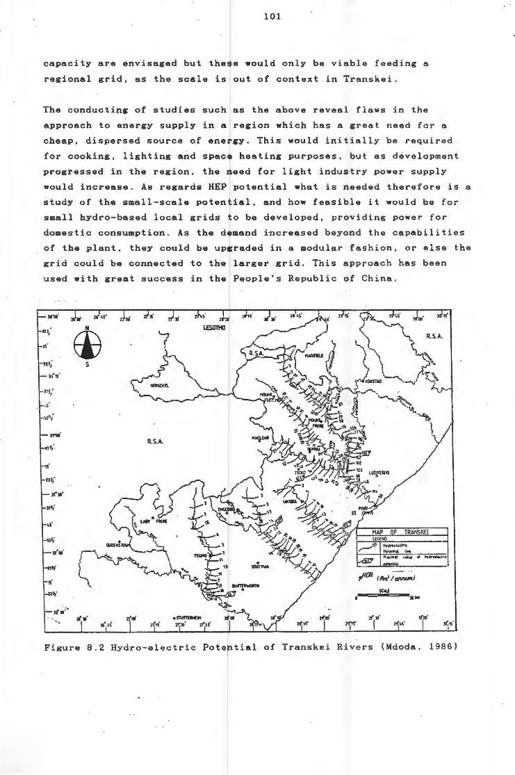
101
capacity are envisaged but these would only be viable feeding a
regional grid, as the scale is out of context in Transkei.
The conducting of studies such as the above reveal flaws in the
approach to energy supply in a region which has a great need for a
cheap, dispersed source of energy. This would initially be required
for cooking, lighting and space heating purposes, but as development
progressed in the region, the need for light industry power supply
would increase. As regards HEP potential what is needed therefore is a
study of the small-scale potential, and how feasible it would be for
small hydro-based local grids to be developed, providing power for
domestic consumption. As the demand i-ncreased beyond the capabi 1 it ies
of the plant, they could be upgraded in a modular fashion, or else the
grid could be connected to the larger grid. This approach has been
used with great success in the People's Republic of China .
Figure 8.2 Hydro-electric Potential of Transkei Rivers (Mdoda, 1986)

102
Another factor to consider is the reliability of the river flow . The
estimates of this should be conservative and the variability of inflow
from year to year should be closely studied . If for instance · the flows
were over-Qstimated then it may be impossible to meet the power
demands even if the hydro station were designed for peak loads only.
During droughts the load factor of a hydro system should be decreased
and in this way the total power demand can still be met. During
periods of high flow the hydro power plants could even be operated on
base load.
A number of micro hydro schemes are in use by farmers in the Eastern
Cape. These have all been built either by the farmers themselves or by
local contractors and are either ROR, or make use of minimal impound
ment. Appendix F lists details of some of those schemes about which
information was able to be found, and is not by any means exhaustive .
8.2.3 Natal
Various studies of hydropower potential have been done in Natal,
mainly looking at the larger scale potential (Langford et al, 1963:
Matthews, 1969; van Robbroeck et al, 1970; Chew and Bowen, 1971). As
mentioned earlier, the only private power company in South Africa
?Perates near Howick, "making use of Francis turbines. There are also a
number of private installations on farms in the Drakensberg . These,
however, represent but a fraction of the hydropower potential.
8.2.4 Eastern Transvaal
No literature on the potential in this region was found , although it
is known that a number of small installations do exist along the
escarpment. Eskom is also involved in the development of a pumped
storage scheme in this area.
8.3 THE ECONOMICS OF SMALL HYDROPOWER IN SOUTH AFRICA
It is in remote underdevelop~d areas that the use of mini and micro
hydro power generation would ~oe most appropriate. Many of these areas
along the previously mentioned 400 km wide strip are still too remote
and sparsely populated to be serviced by the grid. However, the poten
tial exists for small multi-purpose hydro schemes to be developed to
serve the needs of communities. These would include the supply of

103
water for domestic and agricultural use and sufficient power for
lights, water pumping, and possibly some cottage industries. When the
demand for power at such a location increases sufficiently to warrant
extension of the grid, the hydro station would provide voltage stabi
lisation at the end of the line.
As was mentioned earlier, the · above concept has been used with great
success in remote areas of the Peoples' Republic of China, to the
extent that nearly two-thirds of rural Chinese households use electri
city, one-third of which is derived from hydropower (Zhu et al, 1985).
Prior to 1949, the total installed small hydropower (SHP) capacity was
3 634 kW, which has now risen to close to 10 000 MW, 5 910 MW of which
is connected to the grid (Bai, 1985). Of great assistance in the
development of this potential has been the coordinated effort on the
part of the water and power supply authorities. Whenever dams are
constructed for irrigation purposes, space is left in the civil engin
eering works for the installation of hydropower equipment. There has
also been a concerted effort to standardise on the equipment itself,
thus greatl~ facilitating its design, construction and maintenance.
Generally speaking, the smaller the hydropower scheme under consider
ation, the higher the specific ~osts, i.e. per kW installed, are
~ikely to become. However, the costs will, especially in the case of
small scaLe HEP projects be very much project specific. This is as a
result of the wide range of civil works that may be necessary, and
will thus vary from project to project. This was definitely found to
be the case with the micro-hydro schemes investigated in South Africa.
As site-related i.e. civil costs can be expected to be between 50% and
70% of project costs on many HEP schemes (Gingold, 1981; Gordon and
Noel, 1986), it can be seen that this variability will have a signifi
cant effect on the overall cost of a project.
The cost of the equipment, including the turbine, generator and trans
mission equipment can be expected to constitute a further 20% to 40%
of project costs with the last 5% to 15% devoted to engineering costs
(Gingold, 1981; Gordon and Noel, 1986). An approach often used in the
initial costing of HEP equipment for a particular scheme, is that of
applying an empirical specific cost correlation, based on the cost of
previous projects. A review of costs internationally has shown that
the development of a hydropower site requires a certain minimum sum
(Gordon and Noel, 1986). This minimum cost can be related to a func-
104
tion of available head, and generating capacity. Gordon and Noel deve
loped such a correlation.
8.3.1 The Economics and Use of Small Hydropower in South Africa
The ab6vementioned correlation of Gordon and Noel has been adj~sted
for South African conditions by Hoy (1987). This correlation, which
will be used for the calculation of project costs in this report is as
follows:
C: 18 750 * kW 0 ·•a * h-o,a••
where:
C = minimum capital cost in R
kW = installed capacity of turbine in kW
h = net head in meters
This function applies in the case of small i.e. 1 - 100 MW hydropower
projects designed to the high standards required for the generation of
reliable power. If, on the other hand, a micro hydro project is being
considered, and the level of reliability required is not according to
normal grid specifications, then lower design standards can be
~pplied. In such cases costs can be cut by a factor of two or more,
especially if most of the civil works ~re undertaken by the owner .
The potential for the use of small scale hydropower by farmers and
remote communities in South Africa has been recognised by a number of
small entrepreneurs . Two of these were visited during the course of
the project, and data on their various installations were collected.
The plant ranged in size from 0,25 kVA to 54 kVA, and were all robust
in design, and entirely appropriate to the technological skills of
their operators.
The largest installation, designed and built by Mr P. Downey of
Hofmeyr, is situated not far from the outlet of the Orange-Fish
Tunnel. It is thus assured of a steady water flow for all but three
weeks of the year, when the tunnel is emptied and inspected. The
turbine is of the crossflow type, and utilises a head of 7,3 m and a
flow of 1300 1/s. The power generated by it supplies all the domestic
needs of two homesteads, lighting and hot water for 14 labourers
cottages, and all the power requirements of a workshop and fodder
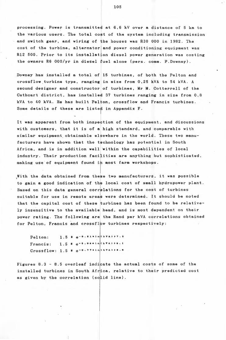
105
processing. Power is transmitted at 6,6 kV over a distance of 5 km to
the various users. The total cost of the system includ i ng transmission
and switch gear, and wiring of the houses was R30 000 in 1982 . The
cost of the turbine, alternator and power conditioning equipment was
R12 500. Prior to its installation diesel power generation was costing
the owners R6 000/yr in diesel fuel alone (pers . comm. P.Downey).
Downey has installed a total of 15 turbines, of both the Pelton and
crossflow turbine type, ranging in size from 0,25 kVA to 54 kVA. A
second designer and constructor of turbines, Mr M. Cotterrell of the
Cathcart district, has installed 37 turbines ranging in size from 0,8
kVA to 40 kVA. He has built Pelton, crossflow and Francis turbines.
Some details of these are listed in Appendix F.
It was apparent from both inspection of the equipment, and discussions
wi th customers, that it is of a high standard, and comparable with
s i milar equipment . obtainable elsewhere in the world. These two manu
facturers have shown that the technology has potential in South
Africa, and is in addition well within the capabilities of local
industry . Their production facilities are anything but sophisticated,
making use of equipment found in most farm workshops .
,Wi th the data obtained from these two manufacturers, it was possible
to gain a good indication of the local cost of small hydropower plant.
Based on this data general correlations for the cost of turbines
suitable for use in remote areas were determined. It should be noted
that the capital cost of these turbines has been found to be relative
ly insensitive to the available head, and is most dependent on their
power rating. The following are the Rand per kVA correlations obtained
for Pelton, Francis ~nd crossflow turbines respectively:
Pelton:
Francis: 1 . 5 * e-o.eaaan<kYAita.l
Crossflow: 1.5 * e-o.??•ln<kVAI+a . e
F i gures 8.3 - 8.5 overleaf indicate the actual costs of some of the
installed turbines in South Africa, relative to their predicted cost
as given by the correlation (solid line).
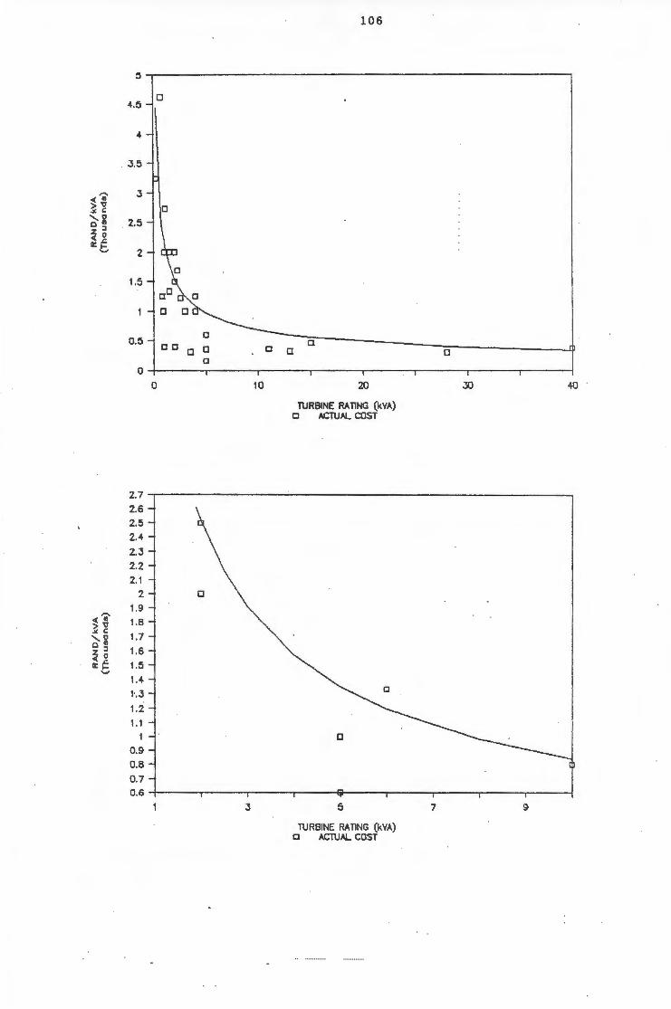
....... <t .. ~~ ,o a ., ~ ~ II:~
'J
,..... < ., >" .X c: "0 a .,
~ ~ II:~
'J
106
0
4.5 0
4
. 3.5
3
2.5
2
1.5 a
0.5 a a a 0 a a D a
04-------~----~~----~-------r------~------r-----~------~ 0
Z.7
2.6 2.5 2.4
2.3 2.2 2.1
2 0
1.9 1.8
1.7
1.6 1.5
1.4 1·.3
1.2 1.1
1 0.9 0.8 0.7 0.6
3
10 20
TURBINE RATING (kVA) a ACTUAL COST
5
TURBINE RATING (kVA) CJ ACTUAL COST
30 40 .
7 9
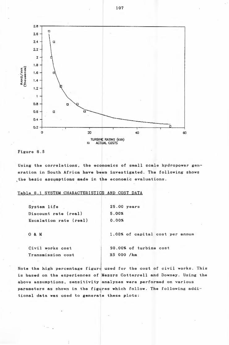
,....., ~~ )I. c: '-.. 0 a " z :I <( 0
~t.
107
Z.8
0 2.6
2.4
2.2
2
1.8
1.6
1.4
1.2
0.8
0.6
0.4
o.z;---------r--------.----7---~------~r--------r--~--~
0 20
'TURBINE RATlNG (kVA) a ACT\JAL COSTS
40 60
F i gure 8 . 5
Using the correlations, the economics of small scale hydropower gen
eration in South Africa have been investigated. The following shows
, the basic ass~mptions made in the economic evaluations.
Table 8.1 SYSTEM CHARACTERISTICS AND COST DATA
System life
Discount rate (real)
Escalation rate (real)
0 &. M
Civil works cost
Transmission cost
25.00 years
5.00%
0.00%
1 . 00% of capital cost per annum
90 . 00% of turbine cost
RS 000 /km
Note the high percentage figure used for the cost of civil works . This
i s based on the experiences of Messrs Cotterrell and Downey. Using the
above assumptions, sensitivity analyses were performed on various
parameters as shown in the figures which follow. The following addi
tional data was used to generate these plots :
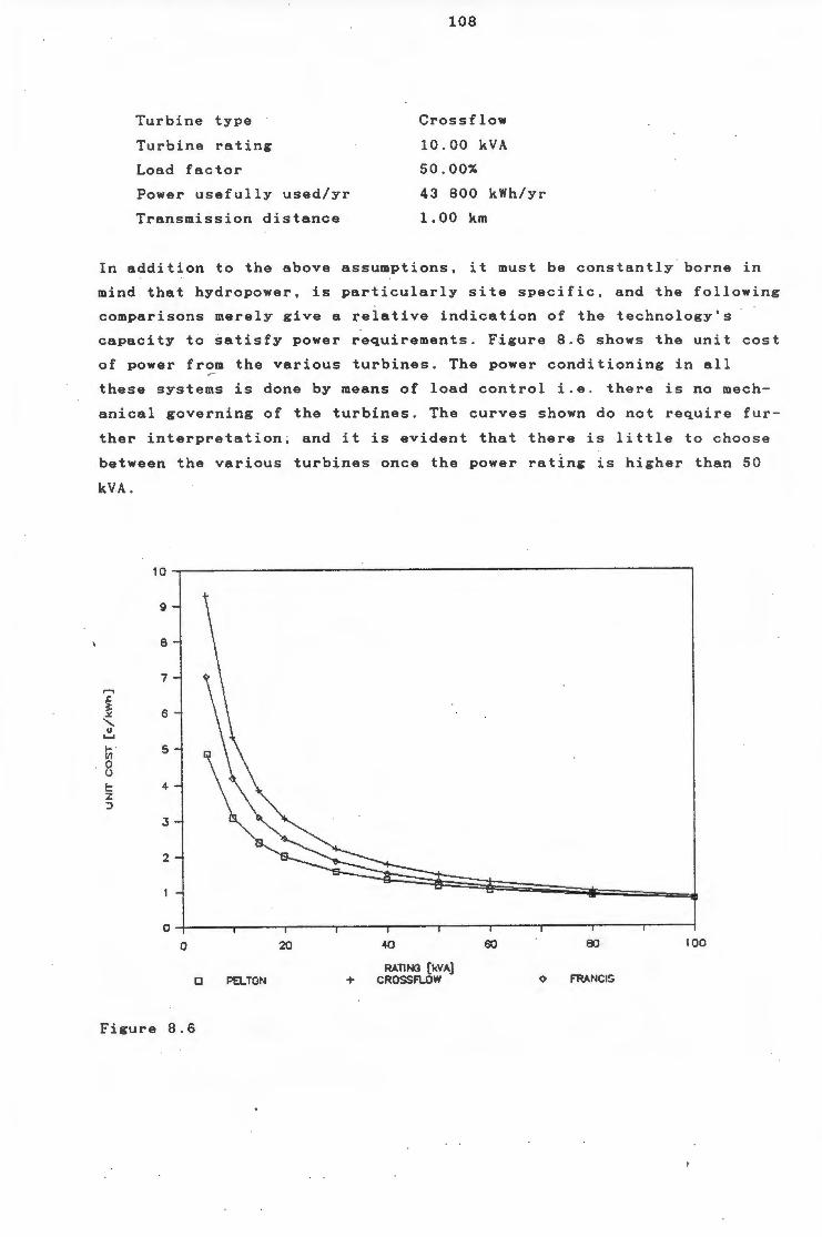
Turbine type
Turbine rating
Load factor
Power usefully used/yr
Transmission distance
108
Crossflow
10.00 kVA
50.00%
43 800 kWh/yr
1.00 km
In addition to the above assumptions, it must be constantly borne i n
mind that hydropower, is particularly site specific , and the following
comparisons merely give a relative indication of the technology ' s
capacity to satisfy power requirements. Figure 8.6 shows the un i t cos t
of power from the various turbines. The power conditioning in all
these systems is done by means of load control i.e . there is no mech
anical governing of the turbines. The curves shown do not require fur
ther interpretation, and it is evident that there is little to choose
between the various turbines once the power rating is higher than 50
kVA .
10
9
8
7 ,...., ~ 6 X.
" 0 ....... f- 5 Ill 0 u f- 4 z :J
3
2
0
0
Figure 8.6
20
PELTON
40
RATING (kVA] + CROSSFLOW
60 80 100
<> FRANCI5
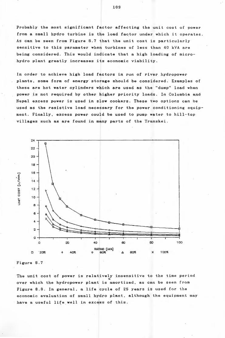
109
Probably the most significant factor affecting the unit cost of power
from a small hydro turbine is the load factor under which it operates.
As can be seen from Figure 8.7 that the unit cost is particularly
sensitive to this parameter when turbines of less than 40 kVA are
being considered. This would indicate that a high loading of micro
hydro plant greatly increases its economic viability.
In order to achieve high load factors in run of river hydropower
plants, some form of energy storage should be considered. Examples of
these are hot water cylinders which are used as the "dump'' load when
power is not required by other higher priority loads. In Colombia and
Nepal excess power is used in slow cookers. These two options can be
used as the resistive load necessary for the power conditioning equip
ment. Finally, excess power could be used to pump water to hill-top
villages such as are found in many parts of the Transkei .
24
22
20
18
,....., 16 l:
\~ 14 ' u .......
.... 12 VI 0 u
10 .... % ::> 8
6
4
2
0
0 20 40 60 80 100
RATING (kVA] 0 ' 2W. + 0 6~ A X 100~
Figure 8.7
The unit cost of power is relatively insensitive to the time period 1!1
over which the hydropower plant is amortized, as can be seen from
Figure 8.8. In general, a life cycle of 25 years is used for the
economic evaluation of small hydro plant, although the equipment may
have a useful life well in excess of this.
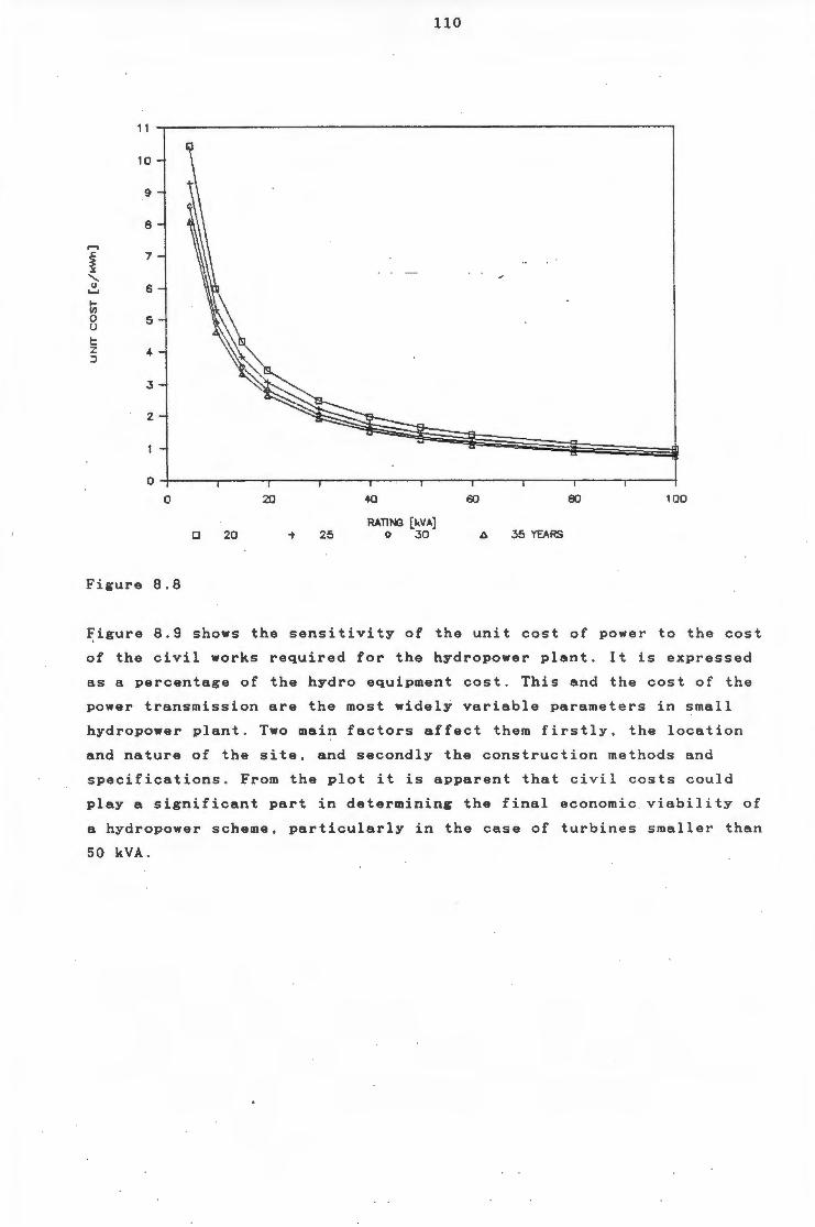
11
10
9
8
,.., ~ 7 ~
' u 6 '-' .... VI 0 5 u .... z :J
4
3
2
0
Figure 8.8
20
0 20 25
110
40
RATING [kVA) 0 JO
60 80 100
35 YEARS
~igure 8.9 shows the sensitivity of the unit cost of power to the cost
of the civil works required for the hydropower plant. It is expressed
as a percentage of the hydro equipment cost. This and the cost of the
power transmission are the most widely variable parameters in small
hydropower plant. Two main factors affect them firstly, the location
and nature of the site, and secondly the construction methods and
specifications. From the plot it is apparent that civil costs could
play a significant part in determining the final economic viability of
a hydropower scheme, particularly in the case of turbines smaller than
50 kVA.
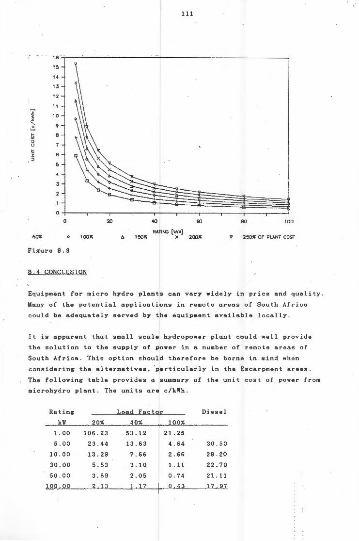
111
16
15 \ 14
13
12
11 ,....., .1:
10 ~ :t. .......
9 u . '--'
.... 8 VI 0
7 u t:
6 z :::>
5
4
3
2
0 ~-----r----~----~------~----~----,-----~-----r----~----~ 0 20 40 60 80 100
RATI~ (kVA) 50% 100~ 150~ X 200~ 7 250~ OF PLANT COST
Figure 8.9
8 . 4 CONCLUSION
Equipment for micro hydro plants can vary widely in price and quality.
Many of the potential applications in remote areas of South Africa
could be adequately served by the equipment available locally.
It is apparent that small scale hydropower plant could well provide
the solution to the supply of power in a number of remote areas of
South Africa. This option should therefore be borne in mind when
considering the alternatives, 'particularly in the Escarpment areas.
The following table provides a summary of the unit cost of power from
microhydro plant. The units are c/kWh.
Rating
kW 20%
1. 00 106.23
5.00 23 . 44
10.00 13.29
30.00 5 . 53
50 . 00 3.69
100.00 2 13
Load Factor
40%
53.12
13.63
7.66
3.10
2.05
1.17
100%
21.25
4.64
2.66
1.11
0.74
0.43
Diesel
30.50
28.20
22.70
21.11
17 . 97
112
CHAPTER NINE
ALTERNATIVELY-FUELLED INTERNAL COMBUSTION ENGINE
POWER GENERATION
Various biomass derived feedstocks can be used to fuel conventional or
modified internal combustion engines. The fuels that will be discussed
in this chapter include gas derived from both the gasification of b i o
mass such as wood, maize cobs and other agricultural residues , and the
gas, also known as biogas, derived from anaerobic digestion of manure
and other agricultural residues .
9.1 THERMAL GASIFICATION OF BIOMASS FEEDSTOCKS
Producer gas has been used as a fuel since the 1920s and during World
War II it was used extensively as a fuel for internal combustion
engines . Small producer gas units were used successfully on trucks and
tractors in Europe and Japan. Interest in it waned when fossil fuels
again became readily available, but was re-awakened with the oil
crises of the seventies . Considerable progress has been made in the
~esign of gasifiers, filtration methods and range of fuels able to be
~sed.
Producer gas is a combination of gases formed by the passage of air
through a bed of hot coals (wood, charcoal, coal etc), into anaerobic
conditions where reduction and cooling then take place . The combust
ible components are formed during the following react i ons :
Carbon monoxide is formed by the partial combustion of
carbon:
2C + Oz : 2CO
Hydrogen and more carbon monoxide is evolved through the
reaction of steam on hot carbon:
Methane is produced by the action of some of the above
hydrogen with hot carbon:
C + Ha : CH•
113
This gives a low calorific value gas with the following typical
analysis by volume:
Carbon monoxide
Hydrogen
Methane
Carbon dioxide
Nitrogen and inerts
20 - 25%
15 - 20%
2 - 4%
10 - 15%
42 - 52%
The effective heat value varies from 3,5 to 6 MJ/m•.
9 .1. 1 Gasification Techniques and Equipment
The best established of all gasifiers are the fixed bed type, also
referred to as vertical shaft gasifiers. There are three basic types,
counter-current, co-current and cross-current (also referred to as up
draught, down-draught and cross-flow). They are generally used for
heating applications, spark and compression ignition, and small spark
ignition engines respectively.
Most gasifiers consist of a hopper containing the feedstock which
gravitates into a chamber in which the processes of drying, pyrolysis.
ox i dation and reduction take place. The ash produced during these '
reactions falls into a lower casing while the resultant gas, at a
temperature of 500-GOOoC, is piped to the cleaning and cooling system.
Some degree of preparation of the feedstock is almost always required,
and may take the form of chopping, hogging, drying and/or briquetting.
Feedstock with a moisture content in excess of 20% is generally
unsuitable since it reduces the high temperatures needed for effective
pyrolysis and tar cracking.
Because the fixed bed gasifier technology is well established for
coal, scale up factors are well-known. All such gasifiers tend to have
certain features in common. They are all able to accept a fairly wide
range of feed sizes, ranging from 10mm up to at least 200mm, although
the quantity of fines (less than 10mm) they can handle is limited to
between 5 and 10% maximum in most cases. Higher levels of fines tend
to block the bed, making gas transfer less even, and increasing the
pressure drop across the bed. Most gasifiers are, however, able to
to l erate fairly high moisture contents, thus allowing the use of
undried biomass .
114
Downdraught Gasifiers
For the 'generation of electricity, the downdraught is the most
commonly used, because of its being particularly suited to most
internal combustion engines. Its major advantage over the updraught
type is that any tars and volatile pyrolysis products must pass the
combustion and reduction zones, and are cracked into fuel gases before
leaving the gasifier.
The downdraught gasifier, however, is sensitive to moisture content ,
and can not accept more than 25% moisture. Several small gasifiers of
this design are known, and were mainly developed during World War II
for use as gas producers for IC engines. They all operate at atmos
pheric pressure, using air/steam as the gasifying agent. More recently
they have found application in small scale power generation. Locally
the National Timber Research Institute (NTRI) has successfully
developed a unit with a thermal output of 1MW.
The main disadvantage of the downdraught mode of operation is that the
drying and distillation occur by radiation and conduction. This,
together with the fact that all the steam produced, must pass through
the gasification zone, means that temperatures are reduced, and more
carbon has to be burnt to counteract these effects. On the other hand
the level of tars and other condensibles are significantly reduced, or
possibly even eliminated. This is due to their being cracked while
passing through the gasification and combustion zones before leaving
the gasifier.
It was generally considered unlikely that downdraught gasification in
fixed beds would develop to any great extent for anything but small
scale gasifiers. However, the NTRI is confident that their successes
will lead to commercialisation of . this technology on both the small
and large scale. Another successful downdraught gasifier is the System
Johansson Wood Gas Producer, developed by Mr KG Johansson of · Halfway
House, Midrand. More details of these will be given later.
Cross-draught Gasifiers
This type of unit was used quite widely in the UK to power vehicles
during World War II. They are not suitable for use with high-tar
fuels, but do allow simple, robust construction. For the former reason
this type of gasifier has proved to be suitable for fuelling with

115
carbonized biomass such as charcoal. They also have operational
advantages with . their quick-start characteristics and rapid responses
to load changes .
Important development of these gasifiers has been done by the Tropical
Development and Research Institute (TDRI). with the specific objective
of . providing a fuel for motive power in underdeveloped countries. This
research has concentrated on small stationary power systems in the 1-
20 kW shaft power output range (Hollingdale et al, 1985). This is
typically the power required by remote communities for maize grinders,
electricity generation and irrigation pumps .
9 . 1.2 Gasifier Feedstocks
Commonly available biomass gasifier feedstocks include wood wastes,
nu t shells, plarit stalks, maize cobs - the list is almost endless . In
most cases the material requires some form of preparation before
gasification, such as size reduction or densification. In addition its
physical and chemical properties (e.g. ash content, total volatiles,
fixed carbon content) must be established, since these factors
strongly influence gasifier design, the gas cleaning train, and the
quality of gas produced. Certain gasifiers, as mentioned above, are
also sensitive to moisture and tar content, so could necessitate the
pr i or carbonisation of the biomass.
Although the carbonisation step may appear to be both an energy and
time consuming operation, it has a number of advantages. Tars and
pyroligneous acids are largely removed in this process, and as a
result the gasifier design is simplified. More consistent gasifier
operation can also be achieved, because of the more uniform nature of
the feedstock.
9 .1. 3 Producer Gas-powered Engines
Although in principle, any internal combustion engine can be converted
to . run on producer gas , in practice, a number of factors which affect
engine choice can be identified. In view of the low calorific value of
the gas, the maximum amount of gas must be drawn into the engine with
each induction stroke. For naturally aspirated engines , therefore,
high volumetric efficiencies should be sought - thus implying slow or
medium speed operation.
116
If 100% operation on producer gas is required, then a spark ignition
engine is needed , with a compression ratio as high as possible , up t o
a maximum of 11:1. A gas/air mixer carburettor must ensure a mixture
ratio of about 1:1 over the required load/speed range . Suitable spark
plugs must be fitted and the ignition timing must take account of the
lower flame speed of producer gas/air mixture compared with the
petrol/air mixture. If the engine is a converted petrol engine , then a
power reduction of 40%, on average, will be experienced when runn i ng
on producer gas .
When operating a gasifier with a ~park ignition engine, arrangements
must be made to start up and sustain the gasifier to the point at
which good quality gas is available (usually about 15 minutes from
ignition). A{ t~is point the engine can be started. This start-up
phase is usually accomplished through the use of a suction fan, hand
or electrically powered, depending on the size of the gasifier .
If a compression ignition engine is to be used, then a substantial
reduction in the consumption of diesel fuel can be achieved . For power
systems below 25 kW, internal engine modifications are often unnecess
ary, an adaptor to connect the gasifier outlet to the engine manifold
,generally being all that is required . If the hydrogen content of the
gas is above about 7%, a change in injection pump timing may be needed
to avoid detonation in the engine cylinders. A timing change is more
likely when using uncarbonised feedstock.
The engine is usually started with 100% diesel fuel and a small pro
portion (10%) is induced through the gasif i er, which is then ignited .
The amount of gas/air mixture drawn into the engine is slowly in
creased over a period of about 15 minutes until about 75 - 80% of the
diesel fuel normally consumed is replaced by gas. Engine speed control
is via the normal diesel pump rack governor.
9.1.4 Case Study of Producer Gas-powered Genset
Extensive tests have been carried out on a prototype System Johansson
gasifier at Halfway House in the Transvaal . This prototype was de -
signed to provide 40 kW shaft brake power at sea level, with the added
criteria that the gas be, as far as is possible , tar free and clean .
Since commissioning in September 1983 this gasifier has provided fuel
for various engi~es for close on 2 500 hours (Johansson , 1986) .
117
The furnace design is somewhat similar to the basic Imbert hearth,
with however, extensive improvements to reduce the loss of heat from
the furnace walls. A high degree of gas cooling and cleaning has been
achieved by the use of a wet scrubber followed by fibreglass filter
media and a finned fan-cooled circulation water cooler. Coarse
particles are removed by a cyclone fitted before the gas scrubber.
Two engines have been tested using the gas alone as fuel, a two litre
Mazda petrol engine with 14,5 kVA alternator, and a 5 litre Chevrolet
V8 with a 37,5 kVA alternator. The Mazda engine had, up to the end of
May 1986, done over 2 200 hours of trouble free running, providing
power for various small workshop machines and domestic use. It
delivers up to 13 kVA at an altitude of 1 500m, with an engine speed
of 2 450 rpm. The Chevrolet has run for about 175 hours, delivering 30
kVA, at an engine speed of 2 150 rpm. Engine speed control is achieved
through double control governors, consisting of a conventional centri
fugal governor, compensated by a commercially available electronic
revlimiter.
The operation of the above gasifier has been monitored by the CSIR,
and extensive analyses of the gaseous products has been carried out.
,Based on these analyses the efficiency of the gas producer has been
determined as 88 - 94% in converting the wood energy into gas energy
(Johansson, 1986). The specific fuel consumption was found to be of
the order of 1,20 - 1,33 kg/kWh. At a woodblock production cost of 3 -
4c/kg, this gives a cost per kWh, including some allowances for waste,
of around 6 - 7c/kWh on fuel costs alone.
9 . 2 BIOCHEMICAL GAS PRODUCTION THROUGH ANAEROBIC FERMENTATION
In the process of anaerobic fermentation, organic matter is completely
degraded to the gaseous products, CH• and COa, with about 90% of the
energy content of the substrate being retained in the methane. Al
though a large amount of organic matter is degraded, only a relatively
low yield of microbial cel~s is obtained. This process is very import
ant for the carbon and nitrogen cycles in nature and it has long been
used for the stabilisation of sewage and other organic wastes. In
addition it has great potential for use in converting biomass sources
such as animal manures, agricultural products and residues, and dome
stic wastes into an energy-rich fuel.

118
Bacteria are primarily responsible for the fermentation, but anaerobic
fermentative protozoa, some anaerobic fungi, and other organisms may
also be important in certain environments. The metabolism and growth
of one species is often dependent on its interactions with other
microbial species. The complete fermentation occurs naturally in a
large number of anaerobic environments that have a slow turnover of
material and where the main electron acceptor, COz, is produced from
the degraded substrates eg . swamps, aquatic sediments of lakes. It
does not occur in environments where other electron acceptors such as
oxygen, nitrate, sulphur or sulphates are readily available .
9.2.1 Biogas Digesters
The above natural process is the subject of ongoing research, but has
been used for many years in the processing of domestic and industrial
sewage. The conventional sewage sludge digester consists essentially
of a completely mixed, one step process operating on a continuous
basis without solids recycle. Due to the low specific growth rate of
the methanogenic bacteria, effective digestion of the waste in a
conventional reactor can only be obtained at long retention times. In
practice, liquid retention times of 20 days or longer are considered
to be essential for efficient waste stabilisation with the result that \
conventional digesters tend to be of large size involving high initial
capital costs.
On the other hand various developing countries have adopted anaerobic
digestion as a means of providing energy in rural areas . The most
publicised of these digesters are those used in rural China , of which
there are reported to be 8 million in use. These were initially con
ceived of as a means of stabilising the sewage of rural communities.
thereby reducing the incidence of disease caused by parasites and
pathogens, but they have subsequently been optimised for the produc
tion of biogas. The Indian gobar (cow dung} gas project, on the other
hand, was initiated with the express intention of producing gas to try
and alleviate rural energy problems.
The Chinese digester has no moving parts, the digester itself acting
as the gasometer, with the liquid level providing the gas compression.
These digesters were originally designed to be operated on a family
basis, or at most with three families and their animals providing the
119
feed for the unit. However, problems with their maintenance, in parti
cular the repair of leaks, has caused many of them to fall into dis
repair. Larger digesters serving a community or village are however
still much in evidence, and make use of separate gas storage tanks,
large polythene balloons being used for this purpose with good
results.
In the 1950s and 1960s a South African pig farmer designed and
operated two large plugflow digesters on his farm near Rustenburg,
obtained a gas yield of 1m 3 /m• digester/day at an operating tempera
ture of 35•C, and retention time of 15 days (Fry, 1974). The yield
drops well below 1m 8 /m'/day if the temperature is not maintained, and
levels of as low as 0,1m• are not unusual. Indeed temperature is one
of the critical parameters determining the performance of a biogas
digester. Any sudden changes in temperature can have disastrous
effects on the bacteria.
The yields obtained from Fry's digester, based on volatile solids fed
to it were as follows. (Volatile solids (VS) is a unit used to measure
that part of the digester feed that is consumed by the microorgan
isms):
Substrate
Pig slurry
Silage effluent
Yield of biogas
0,714 m• of biogas/kg VS
1,1 ditto
Typical values from the literature would be in the range of 0,4-0,5
m2 /kg VS added, using primarily animal manures, human waste and crop
residues as feed, with retention . times of between 10 and 20 days. The
methane content of the gas is usually expected to be about 60%, thus
giving a CH• yield of 0,22-0,3 m8 /kg VS added, over an average reten
tion time of 15 days.
9.2 . 2 Biogas Composition and Cleaning
The major constituents of biogas generated by stable fermentations are
given below:
Constituent
Methane
Carbon dioxide
Moisture
Hydrogen sulphide
Concentration
50-65% by vol
35-50%
30-160 g/m 2
5 g/m•
120
As shown in the table, methane comprises about 50% to 65% of the bio
gas produced during anaerobic fermentation. It is a colourless, odour
less, flammable gas which has an energy value of 37,3 MJ/m'. Natural
gas contains about 95% methane. The critical temperature and pressure
of methane are -82•C and 4,6 MPa, respectively. Thus liquification of
methane is not a practical alternative. Methane is flammable when
mixed with air at concentrations between 5 to 15%, and because of this
caution must be exercised to prevent accidental ignition.
Carbon dioxide is the other major constituent of biogas, and its pre
dominant effect is to dilute the energy value from 37 , 3 MJ/m' to
b_etween 18 and 24 MJ /m 3 , and to increase the volume of gas to be
handled and stored. The lower energy value of biogas decreases the
efficiency of internal combustion engines and requires minor burner
modification for efficient combustion.
Water vapour in the biogas is an important contaminant which must be
removed prior to use in most applications. Condensed water tends to
accumulate in gas handling equipment and meters , causing malfunctions ,
frozen pipes, and corrosion of metal parts when combined with the
hydrogen sulphide and carbon dioxide.
The degree of biogas cleaning needed depends on its eventual applica
tion, the least demanding use being for on-site direct burning. The
minimum requirement in this case is moisture removal to prevent con
densation in gas lines and excessive corrosion. This is of particular
importance when considering its use as a fuel for internal combustion
engines. This can be accomplished by simple frost - proof condensers and
strategically located condensate traps. The concentration of H2S in
the biogas is generally not high enough to be a health or environment
al hazard when oxidised during burning.
In general the removal of carbon dioxide is not done in the case of
small scale digesters, the cost of the equipment being prohibitive on
this scale. The removal of hydrogen sulphide is however advisable. One
of the simplest and most common methods for its removal is the iron
oxide (or iron sponge) process. In this process, the hydrogen sulph i de
reacts chemically with ferric oxide to form ferric sulphide . Regenera
tion is accomplished by passing clean air through the sponge to oxi
dise the ferric sulphide to elemental sulphur and ferric oxide. The \
121
ferric oxide is usually impregnated on wood shavings as a low-cost
medium. Periodically, the ferric oxide must be recharged because the
sulphur accumulation tends to reduce activity and increase the
pressure drop through the bed.
9.2.3 Biogas Use
The two predominant uses of biogas are direct burning and fuelling of
internal combustion engines. Examples of direct burning are for space
heating of residential, commercial, or livestock facilities; crop dry
ing and processing; and steam produ~tion. Use in stationary internal
combustion engines is for prime movers and for generating electricity.
Biogas is unlikely to be used to fuel mobile vehicles on a large scale
because of its relatively incompressible properties. The ulfimate use
of the biogas will depend upon the specific on-site energy require
ments and the scale of operation.
There are several advantages in using biogas as a fuel for internal
combustion engines. Methane has a high octane rating and therefore,
excellent anti-knocking qualities. It mixes well with air and results
in more complete combustion, less residue in oil or exhaust gas. and
less fouling of spark plugs. The only limitations on the use of gases
~n internal combustion engines are that they should be free of dust,
noncorrosive (i.e. less than 1,4 g HaS/m•), not detonate. and not pre
ignite during the compression stroke. The gas can be used directly in
spark-ignition engines, while a pilot quantity of diesel oil is re
quired to provide the ignition in a Diesel cycle engine, as is the
case with producer gas.
The overall efficiency of the internal combustion engine can be
increased by recovering and using the heat losses from the engine. The
recoverable heat as a percentage of the heat input are shown overleaf:
Engine heat losses
Jacket cooling
Exhaust gases
Lubricating oil
Efficiency %
20-30
26-30
1 5-7
These heat losses can be reclaimed as low temperature (75 to 85oC)
process heat, and it is ideally suited to maintaining optimum digester
temperatures for fermentation.
122
During 1985 a University of Cape Town Mechanical Engineering final
year student successfully converted a three-cylinder diesel engine to
run in a dual-fuel mode on biogas produced from chicken manure. Work
is also being done on ~he use of biogas in internal combustion engines
by the Department of Mechanical Engineering at the University of the
Witwatersrand. This includes the use of biogas in both Otto and Diesel
cycle engines. Several dual-fuelled and straight gas engine generators
are in operation at various municipal sewage treatment works around
the country (pers. comm. NIWR).
9.3 THE ECONOMICS OF GAS-FUELLED REMOTE AREA POWER GENERATION
9.3.1 Producer Gas
Although spark-ignition engines can be run directly on producer gas,
the analysis of power costs, from gasifier-powered electricity genera
tion was determined on the basis of a diesel genset . This basis was
used firstly, because of the minimal modification that is required to
diesel engines as compared spark-ignition engines and secondly,
because of the familiarity that exists in remote areas with the use of
diesel engines. As regards the modifications, spark-ignition engines
fequire the addition of some form of speed governing, whereas diesel
engines have an integrated governor.
The gasifier and woodfuel costs used in the evaluations are based on
those given by Johansson (pers. comm . ). The gasifier cost is based on
local production, and is inclusive of all necessary filtering equip
ment. The woodfuel is costed on the basis of wood grown by the user,
and felled and cut into suitable blocks using unskilled labour .
The engine is run such that it uses 10% of its normal diesel fuel as
the ignition source for the producer gas. In the calculations this was
taken as 10% of the power being produced by the diesel component of
the fuel. The table overleaf provides a summary of the basic assump
tions made in the economic evaluation.
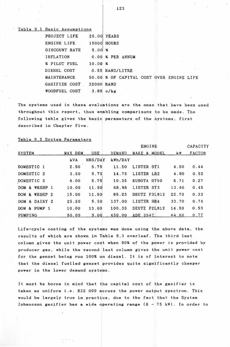
.
123
Table 9.1 Basic AssumEtions
PROJECT LIFE 25.00 YEARS
ENGINE LIFE 15000 HOURS
DISCOUNT RATE 5.00 %
INFLATION 0.00 % PER ANNUM
% PILOT FUEL 10.00 %
DIESEL COST 0.55 RAND/LITRE
MAINTENANCE 50.00 % OF CAPITAL COST OVER ENGINE LIFE
GASIFIER COST 32000 RAND
WOOD FUEL COST 3.85 c/kg
The systems used in these evaluations are the ones that have been used
throughout this report, thus enabling comparisons to be made. The
following table gives the basic parameters of the systems, first
described in Chapter Five.
Table 9.2 System Parameters
ENGINE CAPACITY
SYSTEM MAX DEM USE DEMAND MAKE & MODEL kW FACTOR
kVA HRS/DAY kWh/DAY
DOMESTIC 1 2.50 5.75 11.50 LISTER ST1 4.50 0.44
DOMESTIC 2 3.50 5.75 14.75 LISTER LR2 4.90 0.52
DOMESTIC 3 4.00 5.75 10.35 KUBOTA D750 6. 71 0.27
DOM & WKSHP 1 10.00 11.50 68.98 LISTER ST3 13.40 0.45
DOM & WKSHP 2 15.00 11.50 85.23 DEUTZ F3L912 22 . 70 0.33
DOM & DAIRY 2 25.50 5.50 137.00 LISTER HR4 33.70 0.74
DOM & PUMP 1 10.00 13.00 100.35 DEUTZ F2L912 14.50 0.53
PUMPING 50.00 9.00 450.00 ADE 354T 64.60 0 . 77
Life-cycle costing of the systems was done using the above data, the
results of which are shown in Table 9.3 overleaf. The third last
column gives the unit power cost when 90% of the power is provided by
producer gas, while the second last column gives the unit power cost
for the genset being run 100% on diesel. It is of interest to note
that the diesel fuelled genset provides quite significantly cheaper
power in the lower demand systems.
It must be borne in mind that the capital cost of the gasifier is
taken as uniform i.e. R32 000 across the power output spectrum. This
would be largely true in practice, due to the fact that the System
Johansson gasifier has a wide operating range (8- 75 kW). In order to
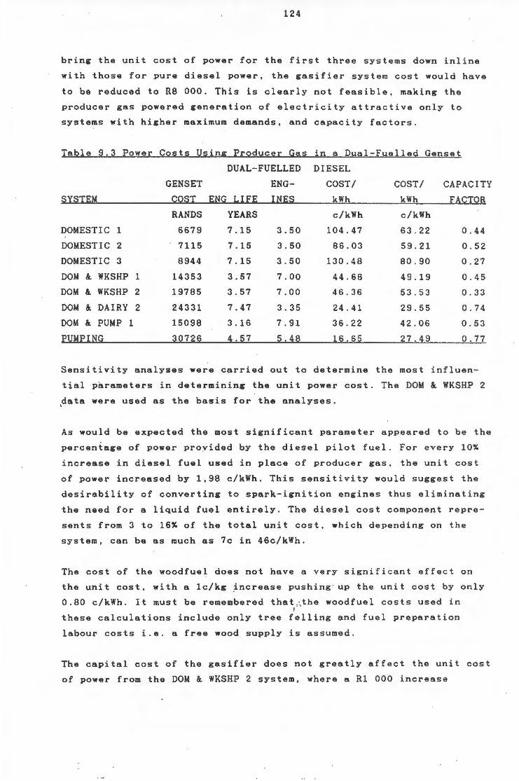
124
bring the unit cost of power for the first three systems down inline
with those for pure diesel power, the gasifier system cost would have
to be reduced to R8 000. This is clearly not feasible, making the
producer gas powered generation of electricity attractive only to
systems with higher maximum demands, and capacity factors.
Table 9.3 Power Costs Using Producer Gas in a Dual-Fuelled Genset
DUAL-FUELLED DIESEL
GENSET ENG- COST/ COST/ CAPACITY
SYSTEM COST ENG LIFE INES kWh kWh FACTOR
RANDS YEARS c/kWh c/kWh
DOMESTIC 1 6679 7.15 3.50 104.47 63 . 22 0 . 44
DOMESTIC 2 7115 7.15 3.50 86.03 59 . 21 0 . 52
DOMESTIC 3 8944 7.15 3 . 50 130.48 80 . 90 0.27
DOM & WKSHP 1 14353 3 . 57 7.00 44.68 49.19 0 . 45
DOM & WKSHP 2 19785 3 . 57 7.00 46.36 53 . 53 0 . 33
DOM & DAIRY 2 24331 7.47 3.35 24.41 29 . 55 0 . 74
DOM & PUMP 1 15098 3.16 7 . 91 36 . 22 42 . 06 0 . 53
PUMPING 30726 4.57 5.48 16.65 27 . 49 0 . 77
Sensitivity analyses were carried out to determine the most influen
tial parameters in determining the unit power cost. The DOM & WKSHP 2
,data were used as the basis for the analyses.
As would be expected the most significant parameter appeared to be the
percentage of power provided by the diesel pilot fuel. For every 10%
increase in diesel fuel used in place of producer gas, the unit cost
of power increased by 1,98 c/kWh. This sensitivity would suggest the
desirability of converting to spark- ignition engines thus eliminating
the need for a liquid fuel entirely. The diesel cost component repre
sents from 3 to 16% of the total unit cost, which depending on the
system, can be as much as 7c in 46c/kWh .
The cost of the woodfuel does not have a very significant effect on
the unit cost, with a 1c/kg increase pushing · up the unit cost by only
0.80 c/kWh . It must be remembered that ~the woodfuel costs used in ' these calculations include only tree felling and fuel preparation
labour costs i . e . a free wood supply is assum~d .
The capital cost of the gasifier does not greatly affect the unit cost
of power from the DOM & WKSHP 2 system, where a R1 000 increase
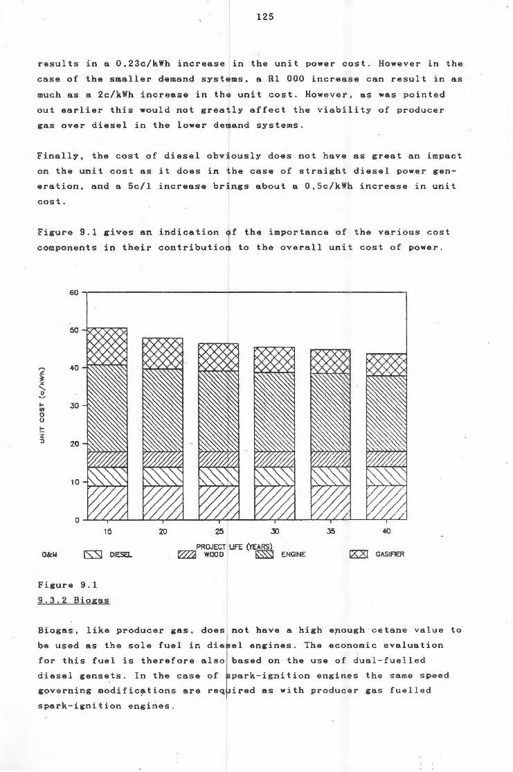
125
results in a 0,23c/kWh increase in the unit power cost. However in the
case of the smaller demand systems, a R1 000 increase can result in as
much as a 2c/kWh increase in the unit cost. However, as was pointed
out earlier this would not greatly affect the viability of producer
gas over diesel in the lower demand systems.
Finally, the cost of diesel obviously does not have as great an impact
on the unit cost as it does in the case of straight diesel power gen
eration, and a 5c/l increase brings about a 0,5c/kWh increase in unit
cost.
Figure 9.1 gives an indication of the importance of the various cost
components in their contribution to the overall unit cost of power.
,..... 40 J:.
~ ~
' ~ 1- .30 (/)
0 0
t: z ;j 20
0&1.1 [SSJ DIESEL
Figure 9.1
9 . 3.2 Biogas
PROJECT UFE (YEA~ ~ WOOD ENGINE l'6:.Z[ G ASI FlER
Biogas, like producer gas, does not have a high epough cetane value to
be used as the sole fuel in diesel engines. The economic evaluation
for this fuel is therefore also based on the use of dual-fuelled
diesel gensets . In the case of spark-ignition engines the same speed
governing modific~tions are required as with producer gas fuelled
spark-ignition engines .
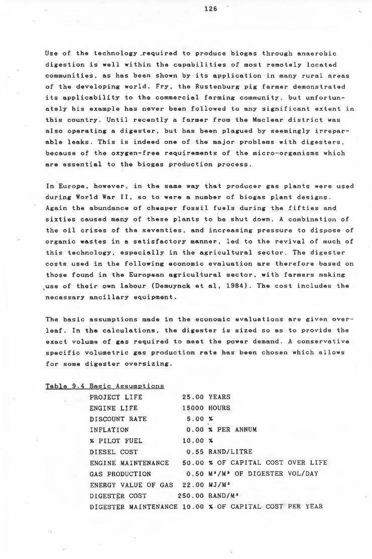
126
Use of the technology .required to produce biogas through anaerobic
digestion is well within the capabilities of most remotely located
communities, as has been shown by its application in many rural areas
of the developing world. Fry, the Rustenburg pig farmer demonstra t ed
its applicability to the commercial farming community, but unfortun
ately his example has never been followed to any significant extent in
this country. Until recently a farmer from the Mac l ear district was
also operating a digester, but has been p l agued by seemingly i rrepar
able leaks. This is indeed one of the major problems with digesters ,
because of the oxygen-free requirements of the micro-organisms which
are essential to the biogas production process.
In Europe, however, in the same way that producer gas plants were used
during World War II, so to were a number of biogas plant designs .
Again the abundance of cheaper fossil fuels during the fifties and
sixties caused many of these plants to be shut down . A combination of
the oil crises of the seventies , and increasing pressure to dispose of
organic wastes in a satisfactory manner , led to the revival of much of
this technology, especially in the agricultural sector. The diges t er
costs used in the following economic evaluation are therefore based on
those found in the European agricultural sector, with farmers making
,use of their own labour (Demuynck et al, 1984). The cost inc l udes the
necessary ancillary equipment.
The basic assumptions made in the economic evaluations are given over
leaf. In the calculations, the digester is sized so as to provide the
exact volume of gas required to meet the power demand. A conservat i ve
specific volumetric gas production rate has been chosen which a l lows
for some digester oversizing.
Table 9.4 Basic Assumptions
PROJECT LIFE 25.00 YEARS
ENGINE LIFE 15000 HOURS
DISCOUNT RATE 5.00%
INFLATION 0.00 % PER ANNUM
% PILOT FUEL 10 . 00 %
DIESEL COST 0 . 55 RAND/LITRE
ENGINE MAINTENANCE 50.00 %OF CAPITAL COST OVER LIFE
GAS PRODUCTION 0 . 50 M3 /M 3 OF DIGESTER VOL/DAY
ENERGY VALUE OF GAS 22.00 MJ/M 3
DIGESTER COST 250.00 RAND/M 3
DIGESTER MAINTENANCE 10.00 %OF CAPITAL COST PER YEAR
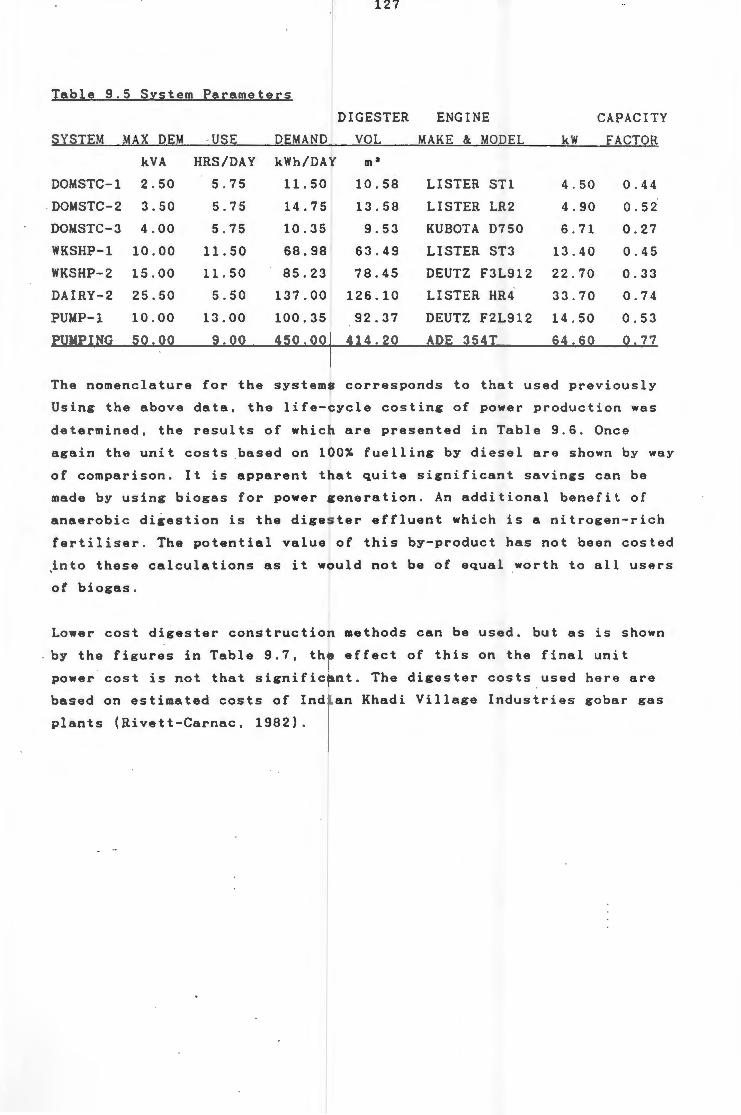
127
Table 9 . 5 S.:Lstem Parameters
DIGESTER ENGINE CAPACITY
SYSTEM MAX DEM USE DEMAND VOL MAKE & MODEL kW FACTOR
kVA HRS/DAY kWh/DAY m•
DOMSTC-1 2.50 5.75 11.50 10.58 LISTER ST1 4 . 50 0.44
DOMSTC-2 3.50 5.75 14.75 13.58 LISTER LR2 4.90 0.52
DOMSTC-3 4.00 5.75 10.35 9.53 KUBOTA D750 6 . 71 0.27
WKSHP-1 10.00 11.50 68.98 63.49 LISTER ST3 13.40 0.45
WKSHP-2 15 . 00 11.50 85.23 78.45 DEUTZ F3L912 22.70 0.33
DAIRY-2 25.50 5 . 50 137.00 126.10 LISTER HR4 33.70 0.74
PUMP-1 10 . 00 13.00 100.35 92.37 DEUTZ F2L912 14.50 0.53
PUMPING 50.00 9.00 450.00 414 . 20 ADE 354T 64.60 0 . 77
The nomenclature for the systems corresponds to that used previously
Using the above data, the life-cycle costing of power production was
determined, the results of which are presented in Table 9.6. Once
again the unit costs based on 100% fuelling by diesel are shown by way
of comparison. It is apparent that quite significant savings can be
made by using biogas for power generation. An additional benefit of
anaerobic digestion is the digester effluent which is a nitrogen-rich
fertiliser. The potential value of this by-product has not been casted
~nto these calculations as it would not be of equal .worth to all users
of biogas.
Lower cost digester construction methods can be used, but as is shown
. by the figures in Table 9.7, the effect of this on the final unit
power cost is not that significant. The digester costs used here are
based on estimated costs of Indian Khadi Village Industries gobar gas
plants (Rivett-Carnac, 1982).
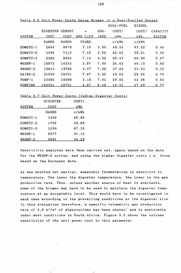
128
Table 9.6 Unit Power Costs Using: Biog:as in a Dual-Fuelled Genset
DUAL-FUEL DIESEL
DIGESTER GENSET ENG- COST/ COST/ CAPACITY
SYSTEM COST COST ENG LIFE INES kWh kWh FACTOR
RANDS RANDS YEARS c/kWh c/kWh
DOMSTC-1 2646 6679 7.15 3 . 50 49 . 24 63 . 22 0 . 44
DOMSTC-2 3394 7115 7 . 15 3 . 50 42 . 43 59 . 21 0 . 52
DOMSTC-3 2382 8944 7.15 3 . 50 69.47 80 . 90 0 . 27
WKSHP-1 15873 14353 3.57 7.00 34.43 49.19 0 . 45
WKSHP-2 19613 19785 3.57 7 . 00 37 . 69 53.53 0 . 33
DAIRY-2 31526 24331 7.47 3.35 19.22 29.55 0 . 74
PUMP-1 23092 15098 3.16 7 . 91 29.02 42 . 06 0 . 53
PUMPING 103551 15701 4.57 5.48 14.31 27.49 0 . 77
Table 9.7 Unit Power Costs (Indian Digester Costs)
DIGESTER COST/
SYSTEM COST kWh
RANDS c/kWh
DOMSTC-1 1409 46 . 86
DOMSTC-2 1706 39.89
DOMSTC-3 1299 67.15
WKSHP-1 5577 31.12
WKSHP-2 6561 34.29
Sensitivity analyses were then carried out, again based on the data
for the WKSHP-2 system, and using the higher digester costs i . e. those
based on the European data.
As was pointed out earlier, anaerobic fermentation is sensitive to
temperature. The lower the digester temperature, the lower is the gas
production rate. Thus, unless another source of heat is available,
some of the biogas may have to be used to maintain the digester temp
erature at an acceptable level. This would have to be investigated in
each case according to the prevailing conditions at the digester site . ·' In this evaluation therefore, a specific volumetric gas production
rate of 0,5 m3 /m 3 of digester/day has been chosen ; and is achievable
under most conditions in South Africa . Figure 9.2 shows the extreme
sensitivity of the unit power cost to this parameter.
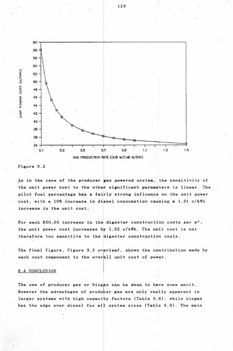
129
60
58
56
54 ""' .c
52 ~ .>/.
' 0 50 "-J
1-Ill 48 0 0
~ IIJ
46 ~ 0 44 Q.
!:: 42 z :I
40
JB
.36
J4 0.1 O.J 0.5 0.7 0.9 1.1 1.J 1.5
GAS PRODUCTION RATE (CUB 1.1/CUB 1.1/0AY)
Figure 9.2
,As in the case of the producer gas powered system, the sensitivity of
the unit power cost to the other significant parameters is linear. The
pilot fuel percentage has a fairly strong influence on the unit power
cost, with a 10% increase in diesel consumption causing a 1,91 c/kWh
increase in the unit cost.
For each R50,00 increase in the digester construction costs per m3,
the unit power cost increases by 1,02 c/kWh . The unit cost is not
therefore too sensitive to the digester construction costs .
The final figure, Figure 9.3 overleaf, shows the contribution made by
each cost component to the overall unit cost of power .
9.4 CONCLUSION
The use of producer gas or biogas can be seen to have some merit.
However the advantages of producer gas are only really apparent in
larger systems with high capacity factors (Table 9 . 8), while biogas
has the edge over diesel for all system sizes (Table 9.9). The main
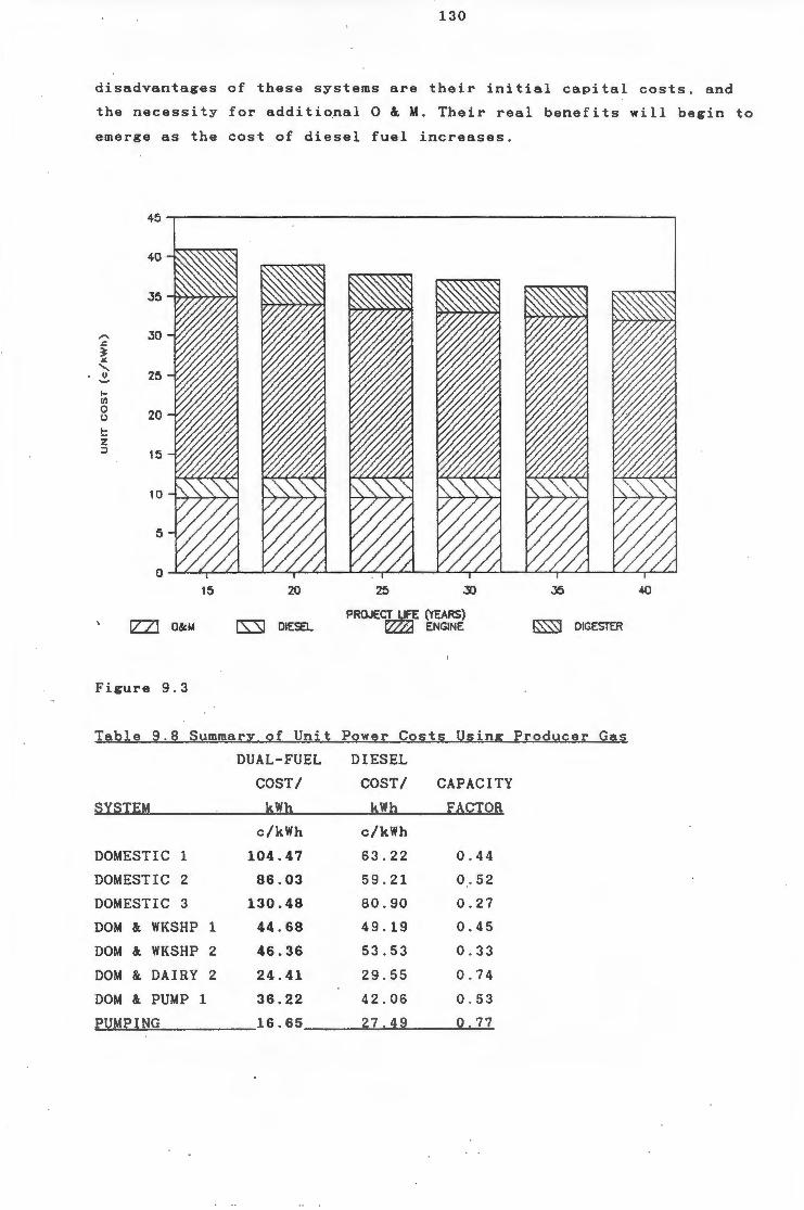
130
disadvantages of these systems are their initial capital costs , and
the necessity for additional 0 & M. Their real benefits will begin to
emerge as the cost of diesel fuel increases.
45
40
35
,..., 30 .t:.
~
"' ' ~ 25 .... (/)
0 20 0
!:: z ::J 15
10
5
0
15 20 25 .3) 35 40
[ZZJ [s::sJ PROJECT UFE (YEARS)
0&1.1 DIESEL I2LZ) ENGINE ~ DIGESTER
Figure 9.3
Table 9.8 Summar;y of Unit Power Costs Using Producer Gas
DUAL-FUEL DIESEL
COST/ COST/ CAPACITY
SYSTEM kWh kWh FACTOR
c/kWh c/kWh
DOMESTIC 1 104.47 63.22 0 . 44
DOMESTIC 2 86.03 59.21 0 . 52
DOMESTIC 3 130.48 80.90 0.27
DOM & WKSHP 1 44.68 49.19 0 . 45
DOM & WKSHP 2 46.36 53.53 0 . 33
DOM & DAIRY 2 24.41 29.55 0 . 74
DOM & PUMP 1 36.22 42.06 0 . 53
PUMPING 16.65 27 . 49 0.77
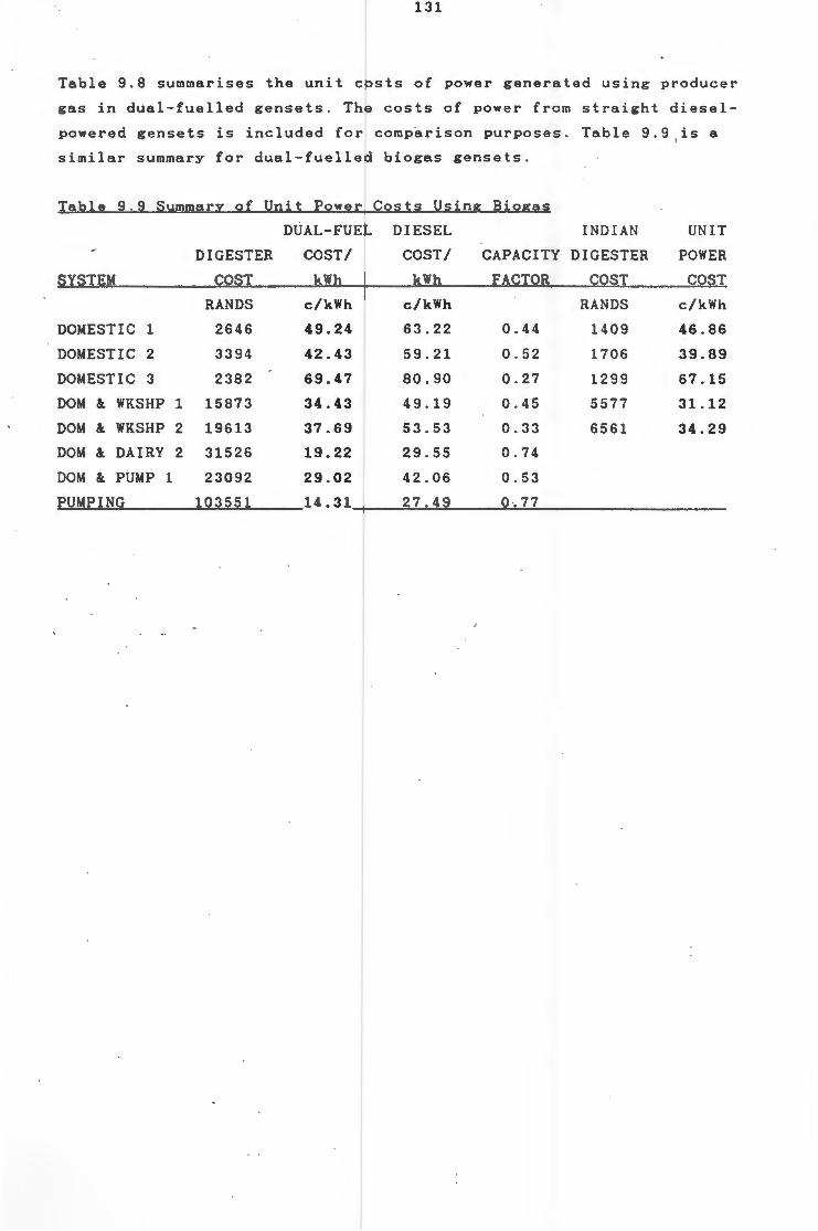
131
Table 9.8 summarises the unit costs of power generated using producer
gas in dual-fuelled gensets. The costs of power from straight diesel
powered gensets is included for comparison purposes. Table 9.9 , is a
similar summary for dual-fuelled biogas gensets.
Table 9 . 9 Summary of Unit Power Costs Using Biogas
DUAL-FUEL DIESEL
DIGESTER COST/ COST/
INDIAN
CAPACITY DIGESTER
SYSTEM COST kWh kWh FACTOR COST
RANDS c/kWh c/kWh
DOMESTIC 1 2646 49.24 63.22 0.44
DOMESTIC 2 3394 42.43 59.21 0.52
DOMESTIC 3 2382 69.47 80.90 0.27
DOM & WKSHP 1 15873 34.43 49.19 0.45
DOM & WKSHP 2 19613 37.69 53.53 0.33
DOM & DAIRY 2 31526 19.22 29.55 0.74
DOM & PUMP 1 23092 29.02 42.06 0.53
RANDS
1409
1706
1299
5577
6561
UNIT
POWER
COST
c/kWh
46.86
39.89
67.15
31.12
34.29
~P~U~M~P~IN~G~------~10~3~55~1 _____ 14.31 ____ _:2~7~·~4~9 ____ ~0~··~7~7-------------------
132
CHAPTER TEN
ANCILLARY POWER GENERATION EQUIPMENT
Given the nature of remote area power supply systems, and in parti
cular,. those using renewable sources of energy, many such systems
require ancillary equipment of various forms and degrees of sophisti
cation. This can basically be divided into two groups, energy storage
equipment and power conditioning equipment. As energy storage is of
such significance, this topic will be dealt with in some detail .
10.1 ENERGY STORAGE
Because of th~ intermittent nature of most renewable energy sources,
one of the most important components in most renewable energy based
power installations is some form of power storage. This storage is
necessary to provide a buffer which will allow the matching of the
energy source with the peak demands of the system being supplied with
power. Thus, for example, the sun's energy received during the day
light hours can be converted into electrical energy through photovol
taic cells, stored in batteries as chemical energy, and then converted
back into electrical energy during the hours of darkness or other
times when it is required.
Pump storage has been mooted as another form of energy storage suit
able for alternative power supply schemes . However this technology is
very much site dependent, and can involve high capital input for a
relatively small storage capacity. This alternative has been investi
gated by the Department of Agricultural Engineering, and is not
recommended as a first option for reasons of cost (pers. comm. ) .
10 . 1.1 Storage Batteries
As batteries can play such an important role in the supply of power in
remote areas, they will be dealt with in some detail. The most common
form of storage used in renewable energy installations at present is
the secondary (or rechargeable) storage battery. A secondary storage
battery consists of an assemblage of cells that are chemically revers
ible ·to a degree that permits electrical recharging. In this report
133
the term battery will be used to exclusively denote an assembly of
electrochemical cells electrically connected in series.
By way of explanation, a primary battery system is one in which the
reagents contained in the constituent cells are the source of electri
cal energy e.g. torch battery. A secondary battery on the other hand
depends on electrical energy initially being produced elsewhere by
some form of electrical generator. For detailed explanations of the
electrochemistry and construction of batteries, the reader is referred
to the many specialist texts on the subject.
Despite the great deal of research that has been done into batteries,
their construction and characteristics, they probably constitute the
most complex and sensitive component of a renewable power supply
system. As lead-acid batteries are the most commonly used storage
media, this section will discuss their characteristics which are of
importance in their selection and use as stationary power system
storage media.
Battery Design
The electrical energy that a battery delivers during discharge is
derived from the electrochemical reactions taking place between the
electrolyte and the active materials of lead oxide and spongy lead.
The former is held in a paste on the negative plate while the latter
is in the paste of the positive plate. The greater the amount of these
materials the greater will be the capacity of the battery. The theore
tical amounts of active material required for 1 Ah of electricity can
be determined from basic principles, but in reality from three to five
times this amount is used in the construction of the cell.
For a cell to give the maximum output for a given mass of material, it
is essential for the active material to be readily accessible to the
electrolyte. This is achieved by using a large number of thin plates
made up of a lead grid covered with a high ratio of active material to
grid. The same mass of active material distributed in a few thick
plates containing a dense or hard paste would result in a cell of much
lower capacity, because of the reduced accessibility by the electro
lyte. A plate with porous active material is capable of producing a
greater output, particularly at high rates of discharge, than a plate
with a dense, hard, active material. Porosity is achieved by adding
small amounts of carbon or other expanders to the paste mix. Too high
134
a porosity is to be avoided for plates regularly subjected to cycles
of charge and discharge, as this is conducive to short life caused by
premature shedding of the active material .
The formation of lead sulphate during the normal discharge of a ce l l
reduces the porosity of both plates, because of the lead sulphate
occupying more space than the original active material . Normally this
crystalline expansion is taken up by the pores being compressed , and
no harm results. If however, the sulphation is excessive, owing to the
cell being persistently over-discharged and undercharged, or left for
long periods in a discharged condition, the sulphation expands beyond
the normal absorbing ability of the pores . The active material is then
subject to pressure which results eventually in fracture of the grid,
or loss of active material from the plate. If the condition is not
remedied soon enough, the cell loses capacity and will not accept
charge.
The electrolyte used in lead-acid batteries is a solution of pure
sulphuric acid in pure water. It is important that the water used to
top up batteries is either distilled or de-ionised, otherwise contami
nation of the active material can occur, with subsequent reduction in
battery performance and capacity. The water used should therefore meet
the following specifications (Smith, 1980):
Impurity Max . Cone. (ppm)
Chlorin~ 15,0
Copper 10 , 0
Iron 10 , 0
Ammonia 10 , 0
Arsenic 3 , 0
Manganese 0 , 1
Nitrates and nitrites 10,0
Total fixed residue 250,0
Sulphuric acid should only be added to a battery if the specific
gravity of the electrolyte is to be altered, and then only after
consultation with the manufacturer.
135
Rating of Battery Capacity
The capacity of a storage battery may be expressed either as the
ampere-ho~r (Ah) or watt-hour (Wh) capacity. The ampere-hour capacity
is a measure of the electrochemical reaction taking place in the
cells, while the watt-hour capacity is a. measure of the batteries
ability to do work. The watt-hour capacity is obtained by multiplying
the ampere-hour rating by the average value of the voltage during the
discharge period.
In stating the capacity of any battery it is necessary to specify the
rate at which the battery is discharged, the final or cut-off voltage,
the full charge specific gravity and the temperature . These four
factors affect the battery's capacity to a marked degree, that is
apart from other factors related to the design or condition of the
battery.
The most commonly adopted ampere-hour capacity rating is the time
rating. By this it is meant that the capacity of the battery is stated
to be a certain number of ampere-hours that can be delivered within a
specified time. The most commonly used basis is the 8-hour rate which
is used for stationary batteries, while automotive batteries are
customarily rated on a 5-hour rate basis (Willard, - ). Thus the
·capacity of a battery is stated as, for example, 80 Ah at the 8-hour
rate, meaning that the battery can deliver 10 A for 8 hours. At
discharge rates of more than 10 A the battery will provide less than
80 Ah, whilst at rates less than 10 A it will provide more than 80 Ah.
The entire theoretical capacity ~f a battery can not be obtained for
several reasons. The electrolyte does not diffuse into the pores of
the plate with sufficient rapidity, the resistance of the active
material and the electrolyte increases as the discharge progresses,
and finally it is not practical to discharge the battery to zero
voltage. As the the battery discharges, the voltage at the terminals
falls gradually from its open-circuit value until the end of discharge
is approached, at which point it falls much more rapidly.
If a curve is plotted, showing the voltage~ throughout the period of
the discharge, the rapid fall begins at wh~t is commonly known as the
'knee' of the curve. The discharge may be continued slightly beyond
this point, but only a small percentage of the total capacity can be
obtained after the 'knee' is passed. The amount of the actual capacity
136
remaining after the 'knee' depends on the rate at which the battery is
being discharged,· the percentage remaining being greater , the higher
the rate of discharge.
The term final voltage is used to designate the minimum useful and
accepted voltage at various rates of discharge, and is the value at
which the maximum number of ampere-hours can be obtained . It is found
just below the 'knee' of the curves described above, and is lower with
higher rates of discharge. The choice of final voltage will depend
either on the battery application or the discharge voltage character
istics of the battery. For example, a lighting load requires a fairly
high stable voltage and this will be the case with most remote power
supply systems, whilst a heavy engine starting load requires a high
current at a lower working voltage. When final voltage is determined
by the discharge characteristics, it is usually fixed to allow a fall
of 0,3 V/cell from the initial voltage. In the case of most lead-acid
batteries a nominal standard final voltage of 1,75 V/cell is commonly
used (Willard, -).
Most chemical reactions are accelerated at higher temperatures , and
those taking place within an electrochemical cell are no exception. In
addition the resistance and viscosity of the electrolyte are are
reduced at higher temperatures, thus reducing the voltage drop or loss
within the cell and maintaining its terminal voltage at a higher
value. These effects combine to increase a battery's capacity at
higher temperature and reduce it with lower temperature. Because of
the effect of temperature on the internal resistance of the battery,
the capacity varies with the rate of discharge as well . The standard
reference temperature used almost universally is 25oC .
The specific gravity of a cell is a measure of the concentration of
the acid electrolyte contained in it . The value of the specific
gravity when the battery is fully charged is a matter of des i gn and i s
affected by many factors. In the first place the gravity must be high
enough for the electrolyte top contain a sufficient amount of actual
sulphuric acid to fulfill the requirements of the cell. On the other
hand if the gravity is too high the acid content may be strong enough
to have a direct chemical effect on various parts of the c ell.
Between these two extremes there are other factors such as capacity ,
operating temperature, conditions of service and battery life, which
137
dictate the best gravity for the situation. The full charge gravity
most commonly used for heavily worked cycling batteries is 1,290
whereas partially cycled batteries, such as those used for railway car
lighting are run at 1,245 (Willard, -). As the batt~ry discharges the
gravity decreases and can thus be used as an approximate indication of
the state of charge of the battery.
It must be remembered haowever that the specific gravity will vary
with temperature, and therefore corrections must be made for this. The
change is equal to three points (,003) of gravity for every soc change
in temperature (Willard, -). Likewise the gravity will vary as the
electrolyte level falls and rises with the consumption of water
through gassing and evaporation. Both these effects require that a
gravity measurement taken at a specific time should be corrected to
the normal reference temperature of 25°C and normal level. As the
battery ages small losses of acid will occur and result in a slow
decrease in the full charge gravity of the battery.
Given all the above it can now be seen that a battery rating must be
qualified to accurately represent its performance. The following is an
example of a full specification of a particular battery:
12 cell battery with a capacity of 500 ampere - hours at the 8 hour
rate, at a temperature of 25•C, to a final voltage of 1,75 volts
per cell, full charge specific gravity 1,250.
which can be abbreviated to:
12 cell 50 Ah/8 hr/1,75V p.c./25•C/s.g. 1,250
Discharge Characteristics
In general, a battery may be discharged without harm at any rate of
current it will deliver, but the discharge should not, however , be
continued beyond the point where the cells approach exhaustion or
where the voltage falls below a useful value. ~
Discharging at a constant current value, the initial voltage will
depend on the rate of discharge and the normal characteristics of the
cell. As the discharge continues, the cell voltage will slowly
decrease during the first 70 to 80% of the total time period . It will
then fall more rapidly passing over the 'knee' as full time and
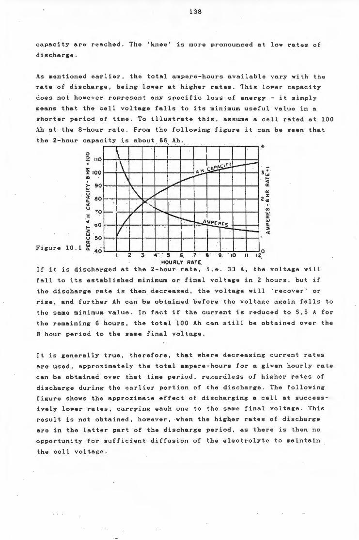
138
capacity are reached . The 'knee' is more pronounced at low rates of
discharge.
As mentioned earlier, the total ampere-hours available vary with the
rate of discharge, being lower at higher rates. This lower capacity
does not however represent any specific loss of energy - it simply
means that the cell voltage falls to its minimum useful value in a
shorter period of time . To illustrate this, assume a cell rated at 100
Ah at the 8-hour rate. From the following figure it can be seen that
the 2-hour capacity is about 66 Ah.
~ \ \
0 o· 110
~ 100 (I)
I
" / _, / ~,
. , I v
>- 90 ... u ~ 80 fl. ~ u .. 0 X: ~ bO ... z w u 51? a:
Figure 10.1 w fl. 40
3 2 I.
~ I P¢ ......-
~~ c~
/ ~ · ~
v ""-
!'-..... r-... ~.41ofpE"REs -..-.::
. . 4 . 5 6, .7 9 ' 10
.HOURLY RATE
-- 3~ ... ~ a: a:
z!
- · II
,. en w a:· w fl. ~ 4
If it is discharged at the 2-hour rate, i . e . 33 A, the voltage will
fall to its established minimum or final voltage in 2 hours, but if
the discharge rate is then decreased, the voltage will 'recover' or
rise, and further Ah can be obtained before the voltage again falls to
the same minimum value. In fact if the current is reduced to 5,5 A for
the remaining 6 hours, the total 100 Ah can still be obtained over the
8 hour period to the same final voltage .
It is generally true, therefore, that where decreasing current rates
are used, approximately the total ampere-hours for a given hourly rate
can be obtained over that time period, regardless of higher rates of
discharge during the earlier portion of the discharge. The follow i ng
figure shows the approximate effect of discharging a cell at success
ively lower rates, carrying each one to the same final voltage. This
result is not obtained, however, when the higQer rates of discharge
are in the latter part of the discharge period , as there is then no
opportunity for sufficient diffusion of the electroly t e to ma i n t a i n
the cell voltage.
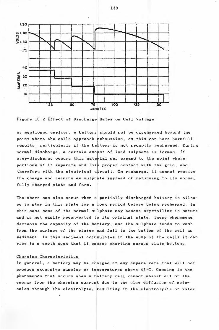
139
1.90 - l ---........... ~ ~ · ~ ,-...
' ~ "' "' "" ' VI 1.85 ~ ~ 1.80
1.75
40
I "' w 30 a: w ' 11. ~ 20 ~
10
I I 25 50 •75 100 150
MINUTES
Figure 10.2 Effect of Discharge Rates on Cell Voltage
As mentioned earlier, a battery should not be discharged beyond the
point where the cells approach exhaustion, as this can have harmful!
results, particularly if the battery is not promptly recharged. During
normal discharge, a certain amount of lead sulphate is formed. If
over-discharge occurs this material may expand to the point where
portions of it separate and lose proper contact with the grid, and
therefore with the electrical circuit. On recharge, it cannot receive
the charge and reamins as sulphate instead of returning to its normal
fully charged state and form.
The above can also occur when a partially discharged battery is allow
ed to stay in this state for a long period before being recharged. In
this case some of the normal sulphate may become crystalline in nature
and is not easily reconverted to its original state . These phenomena
decrease the capacity of the battery, and the sulphate tends to wash
from the surface of the plates and fall to the bottom of the cell as
sediment . As this sediment accumulates in the sump of the cells it can
rise to a depth such that it causes shorting across plate bottoms.
Charging Characteristics
In general, a battery may be charged at any ampere rate that will not
produce excessive gassing or temperatures above 43°C. Gassing is the
phenomenon that occurs when a battery cell cannot absorb all of the
energy from the charging current due to the slow diffusion of mole
cules through the electrolyte, resulting in the electrolysis of water
•
140
into its component gases hydrogen and oxygen at the negative and
positive plates respectively.
The charging of a battery can be divided into three stages, during
which different reactions are predominant:
The efficient charge stage during which the predominant
reactions are the transformation of PbSO. to lead and lead
dioxide. Charge acceptance i . e . that part of the current flowing
through the cell which is used for charging, is ±100% . During
this period, the state-of-charge reaches 70-80%. This stage is
over when the cell voltage reaches 2,35 V and gas evolution
starts.
During the mixed stage water decomposition processes proceed
simultaneously with the charging reactions. The charge acceptance
is gradually and continuously reduced, and the battery is
completely charged at the end of the stage. Cell voltage is
increased from 2,35 V to 2,50 V.
Once the cell is completely charged the gas evolution stage
begins and water decomposition and self-discharge processes begin
in the battery.
Manufacturers of batteries usually specify a normal or 'finish-rate'
in amperes for each type and size of cell made. This rate is a charge
current which can be used safely at any time that charging is
required, and can be continued to the completion of charge without
causing excessive gassing or high temperature . This rate is usually
between 4 and 10 amperes per . 100 Ah of the battery ' s 8-hour capacity,
depending on the cell structure and battery assembly. Where a number
of high capcity cells are assembled as a battery in close proximity,
the available surface for heat dissipation is reduced and compara
tively lower finish-rates must be used to avoid overheating of the
battery.
A battery which is partially or completely discharged can safely
absorb much higher currents than the finish-rate , up to possibly 10
times that value, but as full charge is approached, the current must
be reduced, either gradually or in one or more steps, to the finish
rate or less. In practical applications, it is seldom necessary to use
141
currents of more than 4 or 5 times the finish-rate to charge in the
time available. When the charge is complete, it should be stopped or
reduced to a very low value.
In any type of service under- or over-charging of a battery should be
avoided. An insufficient char~e, even to a small degree - but
continued, will cause gradual sulphation of the negative plates with
eventual loss of capacity and reduction of battery life. An excessive
amount of charge results in the grids of the positive plates 'forming
up' into lead peroxide, physically weakening them and increasing their
resistance. If the overcharging is at a comparatively high rate,
excessive gassing will result tending to wash active material from the
plates. All of these effects reduce the life and efficiency of the
battery.
10.1.1.2 Battery Types and Costs
Various types of lead-acid cells are obtainable, but not all are ,
suited to use in power supply systems. The most important character
istic of batteries to be used in such systems is their ability to be
put through numerous cycles of charge and discharge. Typically this
should be in excess of 2 500 cycles o~ 30-50% depth of discharge
without significant loss of capacity_.
Batteries designed to withstand this mode of operation are the so
called tubular cells and traction batteries. Tubular cells are used in
stationary applications for uninterruptable power supplies (UPS), and
backup emergency systems. Traction batteries are used to power milk
floats and forklift trucks, and are thus ideally suited to this mode
of operation. Both these types of battery, if maintained correctly it
is claimed by the manufacturers, can achieve service lives of 10 years
and more.
Automotive batteries on the other hand are designed for shallow
discharges, delivering a high current over a short period . Thus when
operated in a deep discharge cycling mode they deteriorate, and lose
capacity rapidly. Even with careful maintenance t it is doubtful that
they will achieve more than a two year service life.
It is possible however to make relatively minor modifications to auto
motive batteries that would render them more suitable to a cycled mode
142
of operation. These would entail changes in the plate thickness ,
alloys and paste mixtures, enveloping of the plates, alterations to
the electrolyte composition, and a deepening of the battery cas i ng .
This type of modification has been made to automotive batteries i n
Colombia, where they are now widely used by people who do not hav e
access to conventional power sources. Recharging in many areas is
achieved through the use of micro-hydro power, while in others PV
cells are used. Unfortunately details of the Colombian initiat i ve have
not been documented, and were received through personal communicat i on .
Special application batteries are currently being developed for PV
power systems in particular. These are in general low-maintenance
,cells, and are presently very expensive, thus placing them out of
contention for most remote area power systems .
In this report tubular cell, traction and automotive batteries have
been used in the economic evaluations of the various remote area power
supply systems. Th~ data used are those supplied by the manufactu r ers
as there is unfortunately very little documented on the expected li fe
of batteries in such systems.
T~~e of Batter~ Cost [Rand] Service life [~ears]
Tubular cell 383 X kWh + 47 . 5 10
Traction 231 X kWh + 52 . 3 1 0
Automotive (Standard} 132 X kWh 2
Enquiries directed to manufacturers· of batteries in Europe met wi th
similar responses, and there is little in the l i terature regard ing
battery performance in smal l remote power systems . A subs i diary o f
Phillips has carried out independent test on a wide range of batteries
for use in photovoltaic systems. However, it is claimed that when the
results were released to the manufacturers they were so alarmed that
they asked that not be released for publication, and that the manufac
turers be given time to rectify the problems identified (pers . comm . ) .
10.2 POWER CONDITIONING EQUIPMENT
The emergence of renewable sources of power has reopened the deba t e on
which is the better option, AC or DC power . Given the losses of power
resulting from the conversion of DC power into AC power, it would seem
.appropriate to be considering the use of DC appliances. Without enter-
143
ing into a lengthy discussion of this subject, suffice it to say that
were DC appliances to be developed alongside lower cost renewable
sources of power such as micro~hydro battery chargers, windchargers
and PV panels, they would be assured of a market in the remote areas
of South Africa.
Having said the above, the principal piece of power conditioning
equipment used in remote power systems is the inverter. It is used to
convert the DC of the storage batteries into the AC required by most
modern appliances. In the past they were principally of the rotary
type, using a DC motor to drive an AC generator to produce constant
frequency AC current. Modern inverters are almost all static, and make
use of solid state components.
Inverters are available in varying degrees of sophistication, ranging
from those that produce a square wave form alternating current through
quasi-sine wave inverters, to those that produce a perfect sine wave.
The first, which is less complex and therefore cheaper than the
others, is suitable for operating many AC appliances, but may cause
overheating in some.
It must also be remembered that inverters are only efficient when
operated at close to their rated capacity, with the efficiency drop
ping off to typically 60% at 50% of rated capacity. The upshot of this
is that they should be sized so as to be operated as close to full
rated capacity as possible. A recommended strategy is to operate as
few AC appliances as possible, and to use accurately sized dedicated
inverters for each of these. This also obviates the necessity to over
size to allow for the surge caused by all inductions motors on the
inverter circuit starting simultaneously. Indeed, most inverters can
deal with a small surge i.e. over rated capacity, for a few seconds,
or even up to a minute.
There are a number of local manufacturers of inverters producing a
range of products suitable for various applications. The principal
market for their equipment is in UPSs for computer installations. The
bulk of the equipment is therefore designed for use in a clean well
controlled environment. It became apparent while rese~rching this
report, that these inverters had, with some exceptions, not performed
to specification when used in the harsher environments found in remote
areas. Certain manufacturers are however making a concerted effort to
144
rectify this situation. The S.A. Bureau of Standards, in conjunction
with some of the local inverter manufacturers is currently developing
performance standards for inverters and UPSs.
An objective of this project was to evaluate locally produced invert
ers. Contact was made with various experts in the field in this
regard, and it was established that this was a rather ambitious unde r
taking . Nonetheless, a microcomputer-based inverter test rig was se t
up at UCT. The main object of the rig was to subject the inverter to
various simulated modes of operation, and to evaluate its performance ,
mainly in terms of its efficiency. The project was plagued by techni
cal problems such as reverse currents emanating from the inverters ,
and was therefore not regarded as reliable enough for use in wi de
scale evaluation of locally available inverters .
The South African Post Office, being a user of inverters , has carried
out its own evaluation of those available locally . However, the engin
eers involved were unable to release the results of their tests. These
tests were also carried out with the view to using the inverters in
UPSs, and so it is doubtful whether they would be applicable to the
less protected harsher conditions found in remote areas.
; 10.3 CHARGE REGULATING EQUIPMENT
It is evident that correct battery charging procedure is important in
ensuring satisfactory battery performance and life. Modern charging
eqipment provides safe and flexible control of battery charging either
automatically or with the minimum of manual attent i on .
In the production of batteries the raw pasted plates are converted to
the active states of lead dioxide and spongy lead in the presence of
dilute sulphuric acid during a process known as formation charge . The
plates are then washed and dried before assembly i n to cells and
batteries. After the addition of the electrolyte and before placing
the battery in service it is then necessary to give the battery an
initial charge. This consists of passing a current into the battery
for a number of hours. This initial charge is very important in that
it serves to complete the electrochemical ~ conve r s i on o f the r ema i n i ng
lead sulphate, thus ensuring that the battery starts its life capable
of delivering the rated capacity.

145
Batteries which are cycled initially increase in capacity by as much
as 10 - 20% more than the nominal capacity. Given that batteries used
in remote area power supply systems are subjected to cycling, it is
l i kely that this phenomenon should occur with them .
10 . 3.1 Battery · Charging Methods
Correct battery charging techniques entail the control of the current
and time of charge to suit the size and operating conditions of the
battery. In the case of a power supply system, the batteries are
usually permanently connected to both the load they are serving and
the source of charging current. However, it is often the case that the
major demand for power is largely confined to one part of the day,
usually the evening. The charging source, however, being from a renew
able source such as solar or wind energy, is intermittent, although in
the former case it is generally more predictable, at least in the
times that it can be expected to be available.
Given the above it is evident that some form of charge and discharge
control is necessary to ensure the satisfactory operation of the
battery system. The basic principle which must be followed during
charge is : maximum admissable current during the efficient charging
period, and optimum low current during the mixed stage. This can be
achieved by applying charging regimes with a versatile profile and
current or voltage control.
Constant-current charging.
The true constant-current method is not necessary for the efficient
charging of batteries and is not widely used. It was used in the past,
mainly because it allowed for quick and accurate determination of the
number of ampere-hours put into the battery.
Constant-voltage charging.
In this case a voltage equivalent to 2,3 to 2,4 V/cell is applied
without any ballast resistance in the circuit. This allows for a large
initial charge current which falls fairly quickly as the back-e.m.f. '
increases, and near the completion of charge, the current falls to a
value less than the finishing rate. This method is quite safe, but is
rarely used for batteries that are deeply-discharged as it requires a
charger capable of a very high output for a short time, and would thus
not be cost-effective. It is used mainly in situations where batteries
a r e discharged no more than 25% of their capacity.
146
Modified constant-voltage charging.
The very large current at the beginning of a constant-voltage charge
makes it necessary to limit the initial or starting current, and to
accomplish this a fixed resistance of small value is placed in series
with the battery.
Controlled current-voltage charging .
During the efficient initial stage of charging constant - current
conditions are used, followed by a crossover to constant-voltage
conditions when a voltage of 2,4 V/cell is reached . The value of the
cell voltage is chosen to give slight gas evolution. The current for
the initial charge depends on the temperature and age of the battery.
For example the current through heated batteries is higher than
through cooled ones. To avoid systematic undercharging of separate
cells in the battery, equalizing charges should be carried out
periodically at higher voltages.
Tapered charging.
In this method the maximum charging current is limited by the voltage
of the cell; Charging commences at the maximum current at a cell
voltage of 2,1 V and is then reduced to a defined value upon the cell
'reaching 2,6 V. Also at a voltage of 2,5 V/cell, the current must not
exceed 8,33% of the 5-hour capacity. Under these conditions, the rate
of gas evolution will not surpass the permissible limit, and no damage
will be caused to the battery. The gassing will however be sufficient
to ensure good mixing of the electrolyte. The correct choice of a
tapered charger depends on the capacity of the battery and the
duration of the process. In order to reduce charging time, a two-step
taper charge can be used, with a higher initial charge current.
Equalizing charge.
A battery is both charged and gas is evolved during the mixed-charge
state. A clear-cut point which defines the end of charging does not
exist. This problem is usually solved by- following manufacturer
recommendations, or through user experience. In addition, the cells
are not always all in an equally charged state . To avoid this charge
mismatch and to ensure maximum life from the battery, manufacturers
recommend that the battery be subjected to a once or twice monthly
equalizing charge . It is essentially a prolonged charge at the
finishing charge rate or less. The equalizing charge is considered
147
finished when the concentration of the electrolyte in each cell
remains the same over a two-hour period, provided the charge current
has been held constant over that period. Equalizing charges tend to
nullify the effects of deep cycling on negative plates, and some
manufacturers recommend that the best means of maintaining plates in a
healthy condition is to subject them to an occasional deep discharges
with a full equalizing recharge.
10 . 3.2 Charging Equipment
Battery charge regulators are made in a wide range of voltage and
current output to suit any number of cells and capacity. Monitoring is
accomplished with sophisticated electronic control, and the termina
tion of the charge when the battery is fully charged is automatic.
A number of local companies are manufacturing the equipment needed for
the monitoring of battery charging in remote power systems. No exten
sive systematic evaluation of this equipment has been done as yet. The
ERI is currently running a number of pilot PV power projects making
use of some of this equipment.
10.4 HYBRID POWER PLANTS
To be effective hybrid power plants rely substantially on much of the
equipment discussed in this chapter, and it is for this reason that
they .are briefly discu~sed here.
In many remote areas the levels of available power from an alternate
resource such as solar radiation, wind or water may be insufficient to
meet the full needs of the consumer. In other cases the cost of the
equipment needed to meet the full power needs at desired level of
reliability may be prohibitively high. To overcome these problems, the
consumer should consider the use of an hybrid power generation system
making use of a combination of power sources, exploiting the strong
and avoiding the weak points of the technologies available .
Clearly, there are no easy rules to follow in selecting an autonomous
power system. Almost every application requires careful analysis. This
involves the examination of the energy resource to be used, investiga
tion of the competitive technologies, and the evaluation of the total
costs over the lifetime of the system. The following are a few hybrid
combinations, and some of the common problems associated with them .
148
10.4.1 PV-Diesel
As has been pointed out already, part of the initial capital cost of a
PV system is generated by the need for autonomy i . e . that it wi ll be
able to support its load under all conditions . This worst-case des i gn
can lead to an extremely high capital outlay . To reduce this cost , a
diesel genset can be used to provide the "cushion", and provide power
during the periods of low insolation . Although the design of such a
system is dependent on a number of factors, the addition of a diesel
genset typically allows a 15 to 20% reduction in array size and a cut
in battery bank by a factor of three or four .
In economic terms, comparing diesel to PV power systems is a trade- off
between operating and initial capital costs. This trade-off will
obviously play a big role in determining the extent to which power
will be provided by each source. As a general rule , loads with small
power requirements are generally best served by standalone PV sys t ems.
In such cases, the array cost saved by hybridization is far exceeded
by the cost of the diesel fuel required. Furthermore, the smallest
diesel genset generates 3 kW, and operating such a machine for a small
load is very inefficient.
Hybrid systems prove the most valuable where reliability is of para
mount importance, such as for telecommunications installations and
remote clinics with operating facilities . They are also cost effective
in areas where available insolation varies greatly. The Western Cape
provides such an example, where the summer insolation levels are h i gh,
but the winter rainfall conditions necessitate large power storage
banks.
10.4.2 Wind-Diesel
Hybrid systems combining wind turbines with diesel generators have a
number of inherent problems. The most important is the fluctuating
character of the wind - variations being of both short and long dura
tion. Because of these fluctuations the available wind power can never
be exactly matched to the demands of the user . Solut i ons to t he above
problem will vary from installation to installation, and are ma i nly
dependent on wind characteristics.
149
In a hybrid system without battery storage, any shortage in wind power
will have to be made up by the diesel genset. If the wind is gusty
i . e. variations are of a short duration, this can result in the diesel
engine running for short periods which is clearly unsatisfactory in
terms of engine efficiency. Such a situation can be dealt with either
by electronically-controlled shedding of unecessary loads, or else by
installing battery storage which would make up the shortfall in power
required. If on the other hand there are long periods of calm, the
diesel genset can probably be run at closer to its optimum efficiency.
This would obviate the need for either load shedding or battery
storage.
The wind characteristics are are obviously the most important factor
in determining the optimum combination of equipment in a hybrid wind
diesel power system. Design of the system therefore depends very much
on the availability of reiiable wind data for the site in question.
10.4.3 Genset-Plus Systems
These are not true hybrid power plants, but embody some of the ele
ments of the philosophy behind hybrids. In these systems an appropri
ately sized battery bank is installed between the diesel genset and
the load. The original diesel could even be replaced with a much
smaller unit as the genset output itself no longer needs to be matched
to the peak demand of the system, but rather the inverter supplying
the power to the system. The diesel genset is now run under complete
electronic control, based on the state of charge of the battery bank .
The engine is run at a specific load to give optimal performance.
Engine running times are reduced to less than one third of those found
under -~irect generator power supply, thus extending time between
replacement or overhaul of the engine.
With the above arrangement the system load can be split, with the 220V
AC loads being supplied via an inverter, while those devices which can
be run off DC power are powered directly from the battery bank. The
battery bank acts as a load levelling device, as peak demands, such as
the power required to start an induction motor, can be provided by the
battery.
Because the need no longer exists to meet the abovementioned peak
demands, the battery charging diesel genset does not need to be as
150
large. Although it is possible to modify existing plant to conform to
the required battery charging criteria, best economy is achieved by
installing smaller, new plant. For example, for a systems with a 20 kW
peak demand an 8 kVA generator set is adequate (Langworthy and Costi,
1983).
Genset-plus systems offer fuel savings of up to 90% over a convention
al diesel installation. Payback of the marginal capital cost of the
engine and charge controller, battery bank and inverter is conceivably
achievable through fuel savings in one year (Langworthy and Co5ti,
1983)
" As mentioned, storage is required in genset-plus systems to even out
the load and to match peak demands, while in wind and photovoltaic
systems it is required to provide power in calm and clouded periods
respectively.
10 . 5 CONCLUSION
It became apparent during the course of this project that the area of
ancillary equipment for alternative power supply systems requires a
research project of its own. This project would look primarily at
batteries, battery protection and charging equipment, and power condi
tioning equipment. This investigation should include that electronic
equipment required for the implementation of hybrid autonomous power
systems.
151
CHAPTER ELEVEN
CONCLUSION AND RECOMMENDATIONS
In general, the overriding considerations in choosing a power source
are its cost and reliability, and most consumers will make a choice
that provides some degree of both. However, the factors which consti
tute the cost effectiveness and reliability of a system are infinitely
more complex than either its initial cost or its robustness.
I t is probably true to say that most decisions regarding remote power
systems are based mainly on consideration of the initial capital cost,
without sufficient awareness of the true running costs. This report
has attempted to analyse the various options available to remote power
consumers in a more holistic fashio~. taking account of all factors .
In this final chapter the various options are compared , as far as is
possible, on an equal basis, bearing in mind the already familiar
r i der regarding the site-specificity of a number of the technologies .
In order to allow some form of comparison the cost of power from the
•various technologies has been calculated on the basis of their provid
ing AC power at a specific level over a 24-hour period. This power is
continuous, except where indicated.
The equipment being compared is as specified in the various chapters
relating to each technology, which is briefly as follows:
Imported:
photovoltaic panels
wind turbines
Locally manufactured:
diesel engines
gasifiers
biogas digesters
hydropower turbines
tubular cell batteries
power conditioning equipment
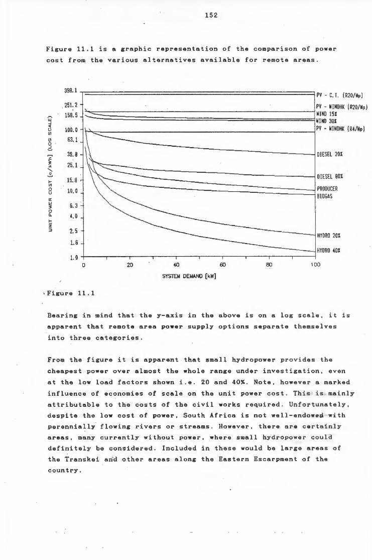
152
Figure 11.1 is a graphic representation of the comparison of power
cost from the various alternatives available for remote areas .
398.1
251.2
,.., 158.5 loJ .J <(
100.0 () (/)
(!) 63.1 0 2-7 39. B :s: 25.1 ;,(.
' C) '-'
.... 15.8 Vl 0 10.0 ()
a:: ~ ? 6. 3 0 0.. 4.0 ~ z ::;! 2. 5
1.6
1.0
1-==================================================1 PV - C. T. ( R20/Wp)
PV - WINDHK (R20/Wp)
..... _"'._::,_ =-:::-=-=-=-:::-=-:::-:::-:::-:::~-=-=-=-=-=-=-=-=-=-=--=-=-=-=-=-=-=-=-=-=-:::-=-=-=-=-=-=-=-=-=-=-=-=-=-=-==1--l WIND 15% WINO 30%
r--"<:;:--------------------------;PV • WINDHK (R4/Wp)
~-------------------_j DIESEL 20%
-- HYDRO 20%
0 20 40 60 80 100
SYSTEM DEMAND (k'N]
' Figure 11 . 1
Bearing in mind that the y-axis in the above is on a log scale, it is
apparent that remote area power supply options separate themselves
into three categories.
From the figure it is apparent that small hydropower provides the
cheapest power over almost the whole range under investigation, even
at the low load factors shown i . e. 20 and 40%. Note, however a marked
influence of economies of scale on the unit power cost . This is mainly
attributable to the costs of the civil works required. Unfortunately,
despite the low cost of power, South Africa is not well-endowed wi th
perennially flowing rivers or streams . However, there are certainly
areas, many currently without power, where small hydropower cou ld
definitely be considered. Included in these would be large areas of
the Transkei arid other areas along the Eastern Escarpment of the
country.
153
The next group of power supply options are the internal combustion
engines fuelled by diesel, producer gas and biogas. The cost of power
from these is roughly an order of magnitude higher than that from the
small hydropower plant. These options can, however, be more economical
than hydropower at low demand levels i.e. around the 5kW demand level.
However, the two straight diesel curves give an indication of the
effect of the load factor on the unit cost of power. It is probably
true to say that the majority of gensets in remote areas are operated
under conditions closer to the 20% load factor curve than the 80%
curve . It is apparent therefore, that wind and PV power are already
wi thin striking distance of conventional diesel power at the lower
demand end of the range.
The most costly category of power supply options are the wind gener
ators and solar photovoltaic systems. The percentages given alongside
the wind curves refer to the turbine capacity factors. Both of the
wind systems are casted on three days of battery storage. It is diffi
cult to determine what LOEP this represents, as it would require an
in-depth analysis of the wind at a particular site .
The PV unit power costs are almost constant over the range 1 - 100 kW .
•This is to be expected given the modular nature of the systems. The
h i gh initial capital cost of the equipment used in wind and PV systems
is the main reason for the high unit power costs shown by these sys
tems. Reduction in the equipment cost will thus have some effect on
the unit cost of power. Th1s is shown, for example, by the curve of
the cost of power from photovoltaic systems sited at Windhoek , assum
ing that the cost per peak Watt of photovoltaic cells were to drop to
R4,00 from the present R20,00 per Wp. (R4,00/Wp is the module price
expected to be achieved in the 1990s).
At the domestic end of the demand range, i.e. 1 - 10 kW, the reduction
in the cost of photovoltaic panels brings the unit cost of power down
to levels competitive with that from diesel engines running at low
load factors . The replacement of batteries is another significant cost
component for both PV and wind systems. It is clear therefore that
effort devoted to developing lower cost energy storage equipment would
y i eld appreciable returns in terms of reduction of unit power costs.
154
When considering the use . of PV systems it must be remembered that at
the small end of the power demand spectrum i.e. less than 2 kW , power
is currently supplied either from petrol powered generators , or from
lead-acid batteries. The cost of power from the former has been calcu
lated to be over RlO,OO per kWh (Muller, 1987). As this was based o n
DC output, it should be compared with a comparable PV system. The
costs in Table 6.6 give the unit cost of DC power from a system cap
able of supplying 10,35 kWh/day as Rl , 94/kWh . Power from the PV sys t em
is thus almost an order of magnitude cheaper than that from the pet r o l
genset.
Lead-acid automotive batteries are used, mainly in peri-urban areas ,
to power television sets and other audio-visual equipment. They are
recharged by local garage or store owners who have access to power .
The economics of battery use in this mode have not been thoroughly
investigated. Costs of recharging in the Western Cape are known to be
between R2,00 and R3 , 00. Assuming a battery life of two years . wh i ch
is optimistic under deep discharge cycling conditions , the un i t cos t
of power is of the order of R2,50 - R3,00 . In practice the cost wi ll
probably be much higher, given that the batteries are generally abused
in the charging and discharging processes. Once again therefore, power
from PV systems provides a cheaper alternative .
It is apparent that a wide spectrum of options exists for power supply
to remote areas of South Africa. Because of a number of factors such
as cheap grid power, past self-generation habits , unfamiliarity with
and high initial costs of alternative energy sources , they have not
been as extensively exploited as they could have been . However , many
of these factors are beginning to lose their impac t . The cost of gr i d
power is increasing in remote areas, both because of longer trans
mission lines and rising generation costs. The diesel fuel price has
increased over the last decade. Both these have resulted in remote
power consumers turning to at least consider alternatives . Those that
could afford them, such as the state and provincial enterprises have
in many cases made the change and thereby shown others the potential
for these alternatives.
Aside from the above, other factors, which can most concisely be term
ed political, have opened up a whole new demand for remote area power
supply. Development of rural areas, mainly populated by subsistence
farmers, has revealed the need for cheap low demand power generation
155
techniques. The characteristics of these areas are very similar to
those of developing regions throughout the so-called Third World, and
the power supply methods used in those instances could provide valu
able pointers.
The power required in these areas has a number of characteristics
which differ from those in the "developed" rural areas. The power
demand is, in general, low and points of consumption are dispersed .
The availability of power is often not crucial, as essential services
are seldom being supplied. It must be pointed out that in the case of
such "unsophisticated" consumers, availability and reliability of
power supply are not synonymous. The remoteness of the areas in
question would require that the equipment be reliable, even though it
need not supply power on demand. An example of this would be a photo
voltaic system sized on ·the basis of a loss of energy probability
(LOEP) of 0,2 or 0,3 rather than the usual 0,1, thus reducing the size
of the array and the battery storage required.
* * * * *
In conclusion, it is hoped that this report highlights some of the
potential for the use of alternative power generation technology in
' South Africa. It should also be stressed that South Africa with its
relatively sophisticated, by Third World standards, manufacturing
industry, is well placed to develop and produce power generation
equipment appropriate to the needs of rural communities .
With the above in mind, the following recommendations are given as
indicators for future research and development in remote area power
supply. These are not ranked in any order of priority, but rather in
the order in which they appeared in the body of the report.
1. It would appear that wind power may have some potential to
supply power in remote areas of South Africa. However, more de
tailed assessments of the wind regimes prevailing in the remote
areas requiring power are
resource can take place.
required before exploitation of this -~
2. The development of lower cost, locally-produced wind turbines
and generators would also greatly facilitate the use of this
resource .

156
3. Extensive irrigation development of South African rivers has
already taken place, but little effort has been made to combine
these developments with the genration of power . In the case o f
straight hydro-electric power (HEP) generation, the cost of power
generation is higher than that from the equivalent thermal power
station, primarily because of the high c i vil works cost
component. However, in a multi-purpose scheme most of t h e c i v il
costs would be borne by the irrigation and water supply component
of the scheme. In addition to new schemes installation of run- o f
river small or micro generators could be considered on exi sting
irrigation schemes.
4. All existing studies on HEP potential have concentrated mainly on
large-scale exploitation, and in general have disregarded small
and micro hydropower. More detailed assessment of this potential
requires surveys of the specific remote areas for which power is
required. This option should therefore be borne very much in mi nd
when considering the alternatives, particularly in the Escarpment
areas, the Ciskei, Transkei and parts of Kwazulu.
5. It became apparent during the course of this project that the
area of ancillary equipment for alternative power supply systems
requires a research project of its own. This project would look
primarily at batteries, battery protection and charging
equipment, and power conditioning equipment. This project should
also investigate the development of lower cost components more
appropriate to the needs of remote rural consumers.
6. While photovoltaics are still expensive, their costs are falling
rapidly and they are finding increasing application in remote
areas, chiefly because of their reliability and low maintenance
requirements. International developments in terms of cost trends
and technology innovation should be tracked and local
applications should be monitored in order to evaluate their cost
effectiveness and also to identify areas which require further
technical research.
~ 7. The cost of power produced from producer and biogas seems
promising and demonstration projects should be supported.
157
REFERENCES
BaiLin (1985), "The role of small hydro in rural electrification",
Water Power and Dam Construction, Feb 1985.
Bester, C.J., Jooste, J.de J., Marshall, D.N. and van Niekerk, B. J .
(1978), Elektrisiteitvoorsiening aan Plase, Departement van
Landbouproduksie-ekonomie.
Borden, C.S. et al (1984), Stand Alone Flat Plate Photovoltaic
Pow~r Systems: Systems Sizing and Life-cycle Costing Methodology
for Federal Agencies, JPL Publications 84-37, Pasadena, USA.
Broome, K.R. (1986), Prefabricated PowerBarge for existing dam
sites, Hydropower, March 1986.
Calloway, T.M. (1985), Design of an Intermediate-Sized, Autonomous
Photovoltaic-Diesel Power Plant, Sandia National Laboratories .
Chew, J . A. and Bowen (1971) , The Water Resources of the Coastal
Areas of Northern Natal and Zululand, Natal Town and Regional
Planning Commission, Vol 17.
Craw~ord, T . S. (1984), Remote Area Power Supply Investigation
(Project RAPS!), State Energy Commission of Western Australia.
Demuynck, M. , Nyns, E.J. and Palz, W. (1984) Biogas Plants in
Europe, D.Reidel Publishing Co, The Netherlands.
Department of Agriculture (1985), Guide to Machinery Costs, P.E.
622/85/2, Directorate of Agricultural Production Economics,
· Pretoria .
De Villiers et al (1984), Report of the Commission of Enquiry into
the Supply of Electricity in the Republic of South Africa, Govt
Printer, Pretoria.
158
Diab, R.D. (1979), Wind Energy Potential over South Africa, Report
submitted to the CSIR, Pretoria .
Diab, R.D. (1986a), Wind Energy Climatology of Natal-KwaZulu ,
Report submitted to the CSIR, Pretoria .
Diab, R.D. (1986b), Wind energy resource in South Africa, Conf on
Renewable Energy Potential in Southern Africa, University of
Cape Town, Sept 1986.
Dutkiewicz, R.K.D. (1984), The Potential for Small-scale Hydro
Plant, Proc of Conf on Energy for Underdeveloped Areas,
University of Cape Town, Feb 1984.
Eberhard, A.A. (1983), Alternative Energy Technologies, ERI Report
No 62/02/10.
Eberhard , A.A. (1986), Energy Consumption Patterns in
Underdeveloped Areas in South Africa, Energy Research Institute ,
University of Cape Town.
Evkom (1985), Vordering met verskaffing van elektrisiteit aan
landelike verbruikers gedurende 1985.
Gingold, P.R. (1981), The optimum size of small run-of-river
plants, Water Power and Dam Construction, Nov 1981.
Gordon, J.L. and Noel, R . C.R. (1986), The economic limits of small
and low-head hydro, Water Power and Dam Construction, Apr 1986.
Hansard (1986), Friday, 6th June, p7540.
Hill Kaplan Scott (1979), Electric Load Survey for Transkeian
Government.
Hollingdale, A.C., Breag, G.R. and Pearce, D. (1985), Use of TDRI
cross-draught gasifier for producer gas fuelling of small
engines, Tropical Science, Vol 25, pp51-60 .
Hothershall, R.J. (1984), Micro hydro: turbine selection criteria ,
Water Power and Dam Construction, February 1984 .
159
HoyT. (1987), Unpublished M Sc (Eng) Thesis, UCT.
Johansson, K.G. (1986) Report on long term testing of woodgas
powered engines, Conf. on Renewable Energy Potential in Southern
Africa, University of Cape Town, . Sept 1986.
Langford, C.E.R., Midgley, D.C. and Olivier, H. (1963),
Hydroelectric development of the Tugela River, Tran. S . A. Inst.
of Elec. Eng. Vol 54, Pt 10.
Langford, C.E.R. and Webb, E.F.D. (1970), Survey of usage of hydro
lelectric power with particular reference to small run of river
schemes in S.A., Symposium Water Natal 1970.
Langworthy, A.P. and Costi, J. (1983), Household and homestead
power supply power systems 240/4000 and 240/8000, Remote Area
Power Supply Workshop, Canberra, May 1983.
Matthews, P.E. (1969), Diversion of water to the upper region of
the Tugela Basin, University of Natal.
Mdoda, G.N. (1986), Method for locating sites for hydro-electric
power stations, Conf. on Renewable Energy Potential in Southern
Africa, University of Cape Town, Sept 1986.
Middleton, B.J., Lorentz, S.A., Pitman, W.V. and Midgley, D.C.,
(1981), Surface Water Resources, Volume V, Report No 12/81,
Hydrological Research Unit, University of the Witwatersrand.
Muller, D.H. (1987), The Use of Small Photovoltaic Systems for the
Electrification of Off-grid Homes, Unpublished M.Sc. (Eng.) I • .
Thesis, University of tape Town.
Nielsen Engineering and Research (1978), Wind Power for Farms,
Homes, and Small Industry, U.S. Department of Commerce, National
Technical Information Service.
O'Flynn, D.T. and Darveniza, M. (1978), Requirements of Electricity
Supply to an Individual Domestic Consumer, University of
Queensland, report No EE78/5.
160
Pringle, D.J. (1981), Elektrisiteitvoorsiening aan Plase (Hers i ene
verslag) Departement van Landbouproduksie-ekonom ie .
Rivett-Carnac, J.L . (1982), Biogas- A Literature Rev i ew , Ins tit u t e
of Natural Resources, Unive~sity of Natal.
Roberts , G. (1984), The cost of wind energy in South Africa , Unpub
lished M.Sc . Eng thesis, University of Cape Town .
SAIRR (1983), Survey of Race Relations in South Africa .
Smith,G. (1980), Storage Batteries , Pitman, London.
Solar Energy Intelligence Report (SEIR) (1987), "Luz places SEGS
III and IV into operation on SCE grid", SEIR, V 13 N 1.
Solar Energy Industries Association (SEIA), (1986) , Energy
Innovation: Development and Status of the Renewable Energy
Industries 1985, Vol 1. /
Taylor, R.W. and Stephenson, D. (1986), The appropriate development
of the hydro-electric resources of Transkei, Proc of Conference
on Renewable Energy Potential in Southern Africa, Sept 1986,
University of Cape Town.
Tegen, A.M . et al (1988), Solar Radiation Handbook for Southern
Africa, Energy Research Institute , (in print) .
Thompson, B.W. (1965), The Climate of Africa . Oxford University
Press, pp 2 - 13.
van Robbroeck, T.P.C., Pullen, R.A., Graber, R. and van Schalkwyk ,
(1970), Hydro-electricity, the key to the multi-purpose
development of the Tugela River, Convention: Water for the
Future.
Water Power and Dam Construction (1987) , Small hyd r o potent i al at
large Australain dams, April 1987.
161
Willard, (-), Lead Acid Type Storage Batteries- Fundamental
principles, operation and care (Section 901), Willard Batteries,
Port Elizabeth.
Zhu Xiaozhang, Huang Zhongli and Zhang Zhongyu (1985), "Local grids
based on small hydro stations';, Water Power and Dam
Construction, Feb 1985.
Zweibel, K. (1986), "Photovoltaic Cells", Chem and Eng News, July
7, 1986, V 64 N 27, pp34-48.

APPENDIX A
MAPS OF OFF-GRID AREAS
MAP 1 WESTERN CAPE ESKOM REGION
MAP 2 SOUTHERN CAPE ESKOM REGION
MAP 3 NORTHERN CAPE ESKOM REGION
MAP 4 EASTERN CAPE ESKOM REGION AND THE TRANSKE I
The maps are based on those provided by Eskom .
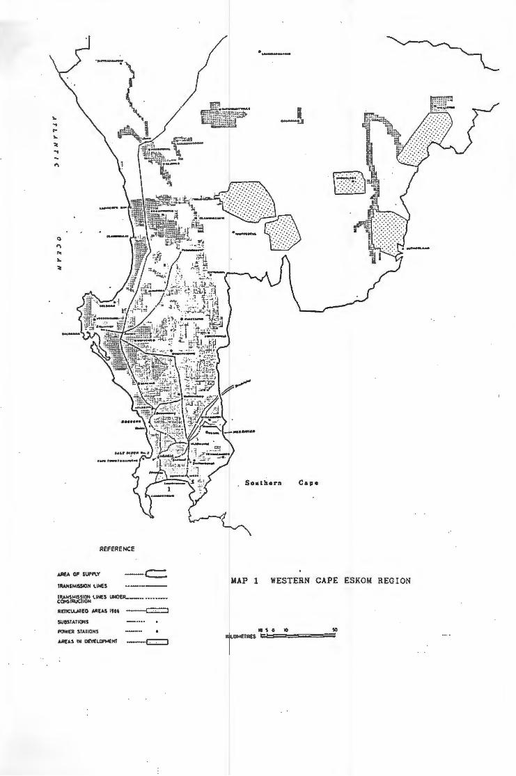
... ... ... ... ~ ... 1"\
Q
1"\
"' ... ~
REFERENCE
AREA OF SUI'f'I.Y
TRANSio<ISSIOH liNES
--c:= TRANSio<ISSION liNES UNDER...-•••• ···•••••• CONSIRUCliON
AETICI.UTED AREAS "" ·-···-c:::::::J SUBSTATIONS
POWER STATIONS
AREAS IN OEVElM<EHT --·c=::J
· ... -.. -·-
Southern Cape
MAP 1 WESTERN CAPE ESKOM REGION
lOS lO 50 KllOio<ETRES i;t:J;i~=;;;l,=s;;=::::=s=;l=s;;::;::;j

I : i : ;,
z 0 ...... t:l t:J a:: :::;: 0 ::.: CJ) t:J
t:J c. < u z a:: t:J ::c !-~ 0 CJ)
N
c. < :::;:
Ill c. ~
0
= ... 41 ... Ill Ill
;:-;
· ~ ......
.....
\J -.. <:; ... .... .. ...
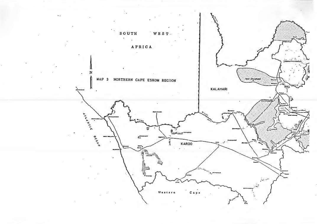
\
' ............
.... ... ... .... 'Z.
~ N
~
... -t'l
MAP 3
0 1"\ ... ....
-,L
SOUTH WEST ·
AFRICA
NORTHERN CAPE ESKOM REGION
KALAHARI
Western C :1 p e
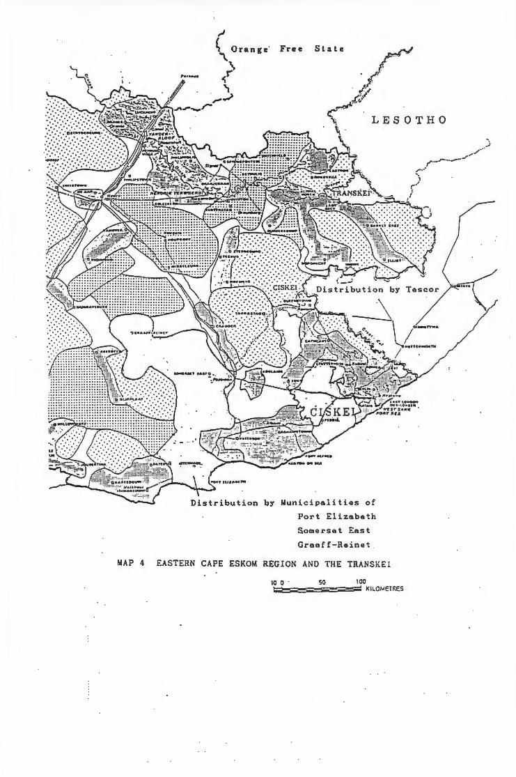
,.1
~ Orange· Free State \
~ ~ ~
LESOTHO
by Municipalities of
Port Elizabeth
Somerset East
Graaff-Reinet
MAP 4 EASTERN CAPE ESKOM REGION AND THE TRANSKEI
10 0 . 50 100 ~--s;;;--=--s:;::: KILOMETRES

APPENDIX B FARM ENERGY SURVEY QUESTIONNAIRES
FARM ENERGY SURVEY {Afrikaans op keersy)
Ha.me of far-.r: .....................•............................................. Address: • ••••••••••••••••••••••••••••••••••••••••••••••••••••••••••••••••••••••••• . . . . . . . . . . . . . . . . . . . . . . . . . . . . . . . . . . . . . . . . . . . . . . . . . . . . . . . . . . . . . . . . . . . . . . . . . . . . . . . . . . . . . . . . . . . . . . . . . . . . . . . . . . . . . . . . . . . . . . . . . . . . . . . . . . . . . . . . . . . . . . . . . . . . . . . . . . . . . . . . . . . . Type of farming operation: •••••••••••••••••••••••••••••••••••••••••••••••••••••••• No of people living on fara: Farmer & family ••••••••••••••••••••••••••••••• Single contract labourers ••••••• Labourers and their families ••••••••••••••••••
Is your fara connected to the ESCOH electricity grid! ••••••••••••••••••••••••••••• If yes, what is the aax1•na power supply! (eg 25kVA, lOOkVA, etc) ••••••••••••••••• How much is your monthly (i) extension charge! •••••••••••••••••••••••••••••••••••
(11) service cbarget •••••••••••••••••••••••••••••••••••. (iii) unit consu.ption charge! ••••••••••••••••••••••••••
Do you use diesel generators? ••••••••••••••••••••••••••••••••••••••••••••••••••••• If yes, what make and capacity diesel generators? ••••••••••••••••••••••••••••••••• . . . . . . . . . . . . . . . . . . . . . . . . . . . . . . . . . . . . . . . . . . . . . . . . . . . . . . . . . . . . . . . . . . . . . . . . . . . . . . . . . . How old are they? (engine hours)•••••••••••••••••••••••••••••••••••••••••••••••••• How much diesel do you use every .antb for your generators? ••••••••••••••••••••••• And bow .uch is used each month for other fara aac:hinery and vehicles! •••••••••••• How much do you pay for the diesel? ••••••••••••••••••••••••••••••••••••••••••••••• Do the generators start autoaatically once power is dravnt •••••••••••••••••••••••• Or are the generators run for a specific period each dayt ••••••••••••••••••••••••• How many hours do they run each dayt •••••••••••••••••••••••••••••••••••••••••••••• What capacity batteries do the generators charge? ••••••••••••••••••••••••••••••••• How regularly do your generators require aaintenancet •••••••••••••••••••••••••••••
Do you use a wind generator, solar cells, water turbine, wood gasifier, etc to ,generate electricity? •••••••••••••••••··If yes, give details: ••••••••••••••••••• ...................................................................................
Apart froa household purposes, do you use electricity for irrigation, agricultural processing, workshops, etc? ••••••••••••••• If yes, give details: ••••••••••••••••• .................................................................................. . . . . . . . . . . . . . . . . . . . . . . . . . . . . . . . . . . . . . . . . . . . . . . . . . . . . . . . . . . . . . . . . . . . . . . . . . . . . . . . . . .
For water pumping do you use {state number): vindaills diesel puaps ••••••• band puaps •••••• solar p~s •••••• .aiDs electricity ••••••• other ••••••••••••••
What do your labourers use for electricity cooking and beating? lighting? If possible, state bow much is used each month:
wood coal
If firewood is used, is it froa: a farm plantation?
paraffin gas other
or natural bush?
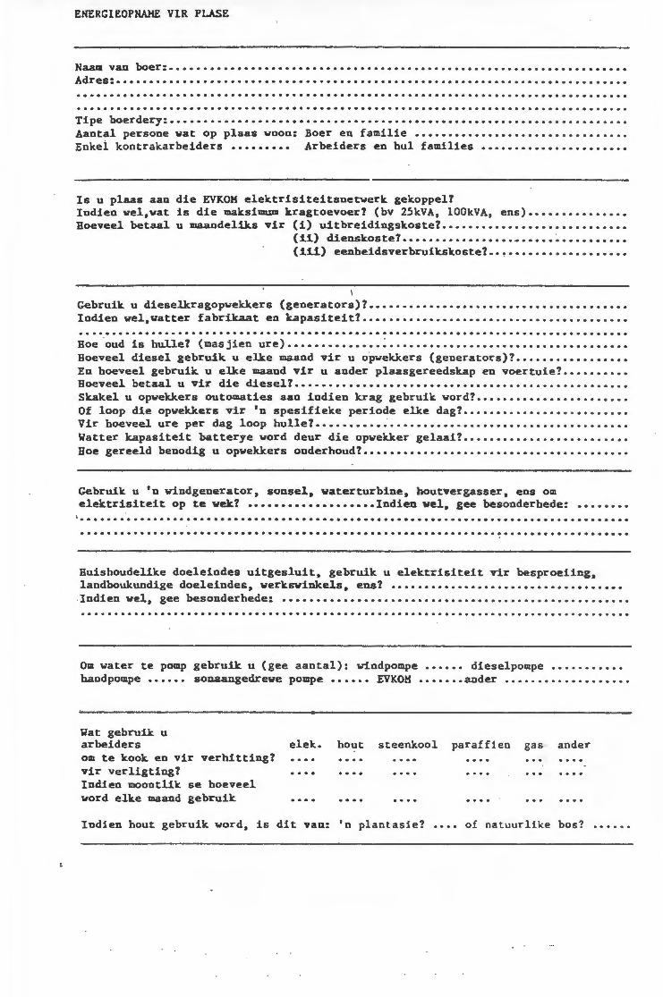
ENERGIEOPNAHE VIR PLASE
Naam van boer: •.•.•••••••••••.••.••.•••••••••••••.••.•.••.••.•....••.•.•••••.••••• Adres: ..•.•..•••••••..•••••••••••••.••.•••••.•••••••••.••••.......••.......•••..•• . . . . . . . . . . . . . . . . . . . . . . . . . . . . . . . . . . . . . . . . . . . . . . . . . . . . . . . . . . . . . . . . . . . . . . . . . . . . . . . . . . . . . . . . . . . . . . . . . . . . . . . . . . . . . . . . . . . . . . . . . . . . . . . . . . . . . . . . . . . . . . . . . . . . . . . . . . . . . . . . . . . . Tipe l>oerdery: ............••..•••••••..•.......•.•••.••.••............ • ... . ... •. •• Aantal persone wat op plaas woon: Boer en familie •••••••••••••••••••••• •••• •••··· Enkei kontrakarbeiders ••••••••• Arbeiders en bul families ••••••••••••••••••••••
Is u plaas aan die EVKOM elektrisiteitsnetwerk gekoppel7 Indien wel,vat is die maksimum kragtoevoer7 {bv 25kVA, lOOkVA, ens) ••••• •••••••• •• Boeveel betaal u maandeliks vir (i) uitbreidingskoste? ••••••••••••••••• ••••• ••••••
(~i) dienskoste? •••••••••.•.••••••••••• ~ •••••••••• (iii) eenbeidsverbruikskoste? •• , ••••••••••••••••••
Gebruik u dieselkragopwekkers (generators)? ••••••••••••••••••••••••••••••••••••••• Indien wel,vatter fabrikaat en kapasiteit? ••••••••••••••••••••••••• •• ••••••••••••• . . . . . . . . . . . . . . . . . . . . . . . . . . . . . . . . . . . . . . . . . . . . . . . . . . . . . . . . . . . . . . . . . . . . . . . . . . . . . . . . . . Boe oud is bulle? (mas jien ure) •••••••••••••• ~ •••••••••••••••••••••••••••••••••••• Boeveel diesel gebruik u elke maand vir u opwekkers (generators)? ••••••••••••••••• En boeveel gebruik u elke maand vir u ander plaasgereedskap en voertuie? •••••••••• Boeveel betaal u vir die diesel? •••••••••••••••••••••••••••••••••••••••••••••••••• Skakel u opwekkers outomaties aan indien krag gebruik word? ••••••••••••••••••••••• Of loop die opwekkers vir 'n spesifieke periode elke dag? ••••••••••••••• •• ••• •••• • Vir boeveel ure per dag loop bulle? •••••••••••••••••••••••••••••••••••••••••••• •• • Watter kapasiteit batterye word deur die opwekker gelaai? ••• •••••••••••••••• • ••••• Boe gereeld benodig u opwekkers onderboud? ••••••••••••••••••••••••••••••••••••••••
Gebruik u 'n windgenerator, sonsel, waterturbine, boutvergasser, ens om elektrisiteit op te wek? ••••••••••••••••••• Indien wel, gee besonderbede:
\ ................................................................................. . . . . . . . . . . . . . . . . . . . . . . . . . . . . . . . . . . . . . . . . . . . . . . . . . . . . . . . . . . . . . . . . . . . . . . . . . . . . . . . . . . . Buishoudelike doeleindes uitgesluit, gebruik u elektrisiteit vir besproeiing, landboukuodige doeleindes, werksvinkels, ens? ······················•••••••••••••
.Indien wel, gee besonderhede: •••••••••••••• • ••••••••••••••••····················· ............................................................................. .....
Om water te pomp gebruik u (gee aantal): windpompe •••••• dieselpompe ••••••••••• bandpompe •••••• sonaangedrewe pompe •••••• EVKOM ••••••• ander •••••••••••••••••••
Wat gebruik u arbeiders om te kook en vir verhitting? vir verligting? Indien moontlik se boeveel word elke maand gebruik
elek. bout steenkool
Indien bout gebruik word, is dit van: 'n plantasie?
paraffien gas ander
of natuurlike bos?
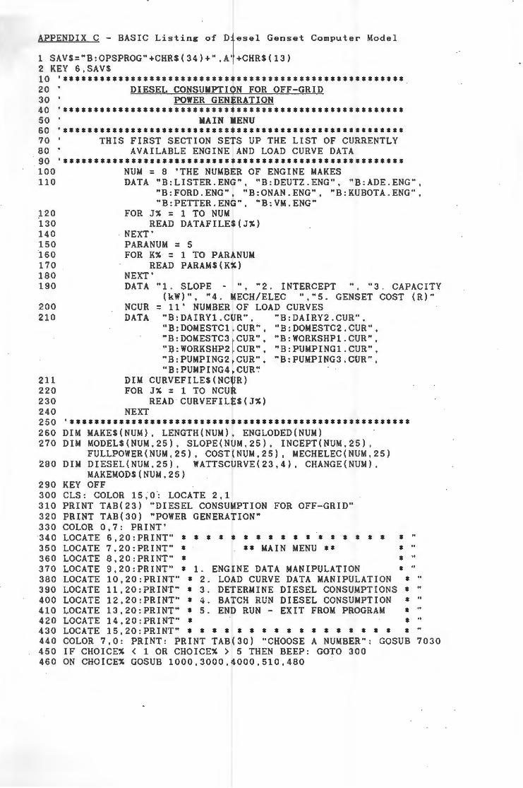
APPENDIX C - BASIC Listing of Diesel Genset Computer Model
1 SAV$:"B:OPSPROG"+CHR$(34)+",A"+CHR$(13) 2 KEY 6,SAV$ 10 '******************************************************* 20 ' DIESEL CONSUMPTION FOR OFF-GRID 30 ' POWER GENERATION 40 .••••••••••••••••••••••••••••••••••••••••••••••••••••••• 50 ' WAIN YENU 60 .••••••••••••••••••••••••••••••••••••••••••••••••••••••• 70 ' THIS FIRST SECTION SETS UP THE LIST OF CURRENTLY 80 ' AVAILABLE ENGINE AND LOAD CURVE DATA 90 '******************************************************* 100 NUM = 8 'THE NUMBER OF ENGINE MAKES 110 DATA "B:LISTER.ENG", "B:DEUTZ.ENG", "B:ADE.ENG",
"B:FORD.ENG", "B:ONAN.ENG", "B:KUBOTA . ENG", "B:PETTER.ENG", "B:VM.ENG"
120 FOR J% = 1 TO NUM 130 READ DATAFILE$(J%) 140 . NEXT' 150 PARANUM : 5 l60 FOR KX = 1 TO PARANUM 170 READ PARAM$(K%) 180 NEXT' 190 DATA "1. SLOPE ~ , "2. INTERCEPT "3. CAPACITY
(kW)", "4. MECH/ELEC ","5. GENSET COST (R)" 200 NCUR: 11' NUMBER OF LOAD CURVES 210 DATA "B:DAIRY1.CUR", "B:DAIRY2 .CUR",
"B:DOMESTC1.CUR", "B:DOMESTC2.CUR", "B:DOMESTC3.CUR", "B:WORKSHP1.CUR", "B:WORKSHP2.CUR", "B:PUMPING1.CUR", "B:PUMPING2.CUR", "B:PUMPING3.CUR", "B: PUMPING4. CUR'.'
211 DIM CURVEFILE$(NCUR) 220 FOR J% : 1 TO NCUR 230 READ CURVEFILES(J%) 240 NEXT 250 '******************************************************* 260 DIM MAKE$(NUM), LENGTH(NUM), ENGLODED(NUM) 270 DIM MODEL$(NUM,25), SLOPE(NUM,25), INCEPT(NUM,25),
FULLPOWER(NUM,25), COST(NUM,25), MECHELEC(NUM,25) 280 DIM DIESEL(NUM,25}, WATTSCURVE(23,4}, CHANGE(NUM},
MAKEMOD$(NUM,25) 290 KEY OFF 300 CLS: COLOR 15,0~ LOCATE 2,1 310 PRINT TAB(23) "DIESEL CONSUMPTION FOR OFF-GRID" 320 PRINT TAB(30) "POWER GENERATION" 330 COLOR 0,7 : PRINT' 340 LOCATE 6,20:PRINT" * * * * * * * * * * * * * * * * * * " 350 LOCATE 7,20 : PRINT" * ** MAIN MENU ** * " 360 LOCATE 8,20 : PRINT" * * " 370 LOCATE 9,20:PRINT" * 1. ENGINE DATA MANIPULATION * " 380 LOCATE 10,20 : PRINT'' * 2. LOAD CURVE DATA MANIPULATION * " 390 LOCATE 11,20:PRINT" * 3. DETERMINE DIESEL CONSUMPTIONS * " 400 LOCATE 12,20 : PRINT" * 4. BATCH RUN DIESEL CONSUMPTION * " 410 LOCATE 13,20:PRINT" * 5. END RUN- EXIT FROM PROGRAM * " 420 LOCATE 14,20:PRINT" * * " 430 LOCATE 15,20:PRINT" * * * * * * * * * * * * * * * * * * " 440 COLOR 7,0 : PRINT: PRINT TAB(30) "CHOOSE A NUMBER" : GOSUB 7030 450 IF CHOICE% < 1 OR CHOICE% > 5 THEN BEEP: GOTO 300 460 ON CHOICE% GOSUB 1000,3000,4000,510,480
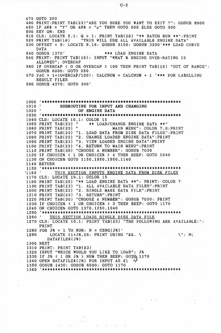
C-2
470 GOTO 300 480 PRINT:PRINT TAB(23)"ARE YOU SURE YOU WANT TO EXIT?": GOSUB 8000 490 IF AN$ : "Y" OR AN$ = "y" THEN GOTO 500 ELSE GOTO 300 500 KEY ON: END 510 CLS: LOCATE 5,1 : Q = 1: PRINT TAB(28) "**BATCH RUN **":PRINT 520 PRINT TAB(16) "THIS WILL USE ALL AVAILABLE ENGINE DATA" 530 OFFSET: 9: LOCATE 8,16: GOSUB 3150: GOSUB 3200'*** LOAD CURVE
DATA 540 GOSUB 1370' *** LOAD ENGINE DATA 550 PRINT: PRINT TAB(16): INPUT "WHAT% ENGINE OVER-RATING IS
ALLOWED"; OVERCAP 560 IF OVERCAP < 0 OR OVERCAP > 100 THEN PRINT TAB(16) "OUT OF RANGE" :
GOSUB 6000: GOTO 550 570 FAC: 1+(0VERCAP/100): CALCNUM: CALCNUM + 1 '***FOR LABELLING
RESULT FILES 580 GOSUB 4370: GOTO 300'
1000 .••••••••••••••••••••••••••••••••••••••••••••••••••••• 1010 ' SUBROUTINE FOR INPUT AND CHANGING 1020 I OF ENGINE DATA 1030 •••••••••••••••••••••••••••••••••••••••••••••••••••••• 1040 CLS: LOCATE 10,1: COLOR 15 1050 PRINT TAB(23) " ** LOAD/CHANGE ENGINE DATA **" 1060 PRINT TAB(23) " MAIN MENU": COLOR 7,0:PRINT 1070 PRINT TAB(23) "1. LOAD DATA FROM DISK DATA FILES'':PRINT 1080 PRINT TAB(23) "2. CHANGE LOADED ENGINE DATA":PRINT 1090 PRINT TAB(23) "3 . VIEW LOADED ENGINE DATA ": PRINT 1100 PRINT TAB(23) "4. RETURN TO MAIN MENU":PRINT 1110 PRINT TAB(30) "CHOOSE A NUMBER": GOSUB 7030 1120 IF CHOICE% < 1 OR CHOICE% > 4 THEN BEEP: GOTO 1040 1130 ON CHOICE% GOTO 1150,1550,1550,1140 1140 RETURN 1150 '*****************************************************
'1160 ' THIS SECTION INPUTS ENGINE DATA FROM DISK FILES 1170 CLS: LOCATE 10,1: COLOR 15 1180 PRINT TAB(25) "** LOAD ENGINE DATA **": PRINT: COLOR 7 1190 PRINT TAB(23) "1. ALL AVAILABLE DATA FILES":PRINT 1200 PRINT TAB(23) "2. SINGLE MAKE DATA FILE":PRINT 1210 PRINT TAB(23) "3. RETURN":PRINT 1220 PRINT TAB(30) "CHOOSE A NUMBER": GOSUB 7030: PRINT 1230 IF CHOICE% < 1 OR CHOICE% > 3 THEN BEEP : GOTO 1170 1240 ON CHOICE% GOTO 1370 , 1250,1040 1250 '***************************************************** 1260 ' THIS SECTION LOADS SINGLE DISK DATA FILE 1270 CLS: LOCATE 10,1: PRINT TAB(23) "THE FOLLOWING ARE AVAILABLE:":
PRINT 1280 FOR J%: 1 TO NUM: N = CSNG(J%)' 1290 LOCATE 11+J%,28: PRINT USING"££. \ \"; N;
DATAFILE$(J%) 1300 NEXT 1310 PRINT: PRINT TAB(23) 1320 INPUT "WHICH WOULD YOU LIKE TO LOAD"; J% 1330 IF J% < 1 OR J% > NUM THEN BEEP: GOT~ 1170 1340 OPEN DATAFILE$ ( J%) FOR INPUT AS £1 -~~ 1350 GOSUB 1430: GOSUB 6000: GOTO 1170 1360 '*****************************************************
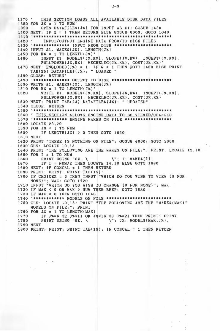
C-3
1370 ' THIS SECTION LOADS ALL AVAILABLE DISK DATA FILES 1380 FOR J% = 1 TO NUM' 1390 OPEN DATAFILE$(J%) FOR INPUT AS £1: GOSUB 1430 1400 NEXT: IF Q : 1 THEN RETURN ELSE GOSUB 6000: GOTO 1040 1410 •••••••••••••••••••••••••••••••••••••••••••••••••••••• 1420 ' INPUT/OUTPUT ENGINE DATA FROM/TO DISK FILES 1430 '************** INPUT FROM DISK ********************** 1440 INPUT £1, MAKE$(J%), LENGTH(J%) 1450 FORK%= 1 TO LENGTH(J%)' 1460 INPUT £1, MODEL$(J%,K%), SLOPE(J%,K%), INCEPT(J%,K%),
FULLPOWER(J% , K%), MECHELEC(J%,K%), COST(J%,K%)' 1470 NEXT: ENGLODED(J%) = 1: IF Q = 1 THEN GOTO 1480 ELSE PRINT
TAB(25) DATAFILE$(J%); "LOADED" 1480 CLOSE: RETURN' 1490 1500 1510 1520
1530 1540 1550 1560 1570 15 80 1590 1600 1610 1620 1630 1640 16 50 1660 1670 1680
'16 90 1700
1710 1720 1730 1740 1750
1760 1770 1780 1790 1800
'************** OUTPUT TO DISK *********************** WRITE £1, MAKES(J%), LENGTH(J%) FORK%= 1 TO LENGTH(J%)'
WRITE £1, MODEL$(J%,K%), SLOPE(J%,K%), INCEPT(J%,K%), FULLPOWER(J%,K%), MECHELEC(J%,K%), COST(J%,K%)
NEXT: PRINT TAB(23) DATAFILE$(J%); "UPDATED" CLOSE: RETURN '***************************************************** ' THIS SECTION ALLOWS ENGINE DATA TO BE VIEWED/CHANGED '************* ENGINE MAKES ON FILE ****************** LOCATE 23,20 FOR J% = 1 TO NUM
IF LENGTH(J%) > 0 THEN GOTO 1630 NEXT PRINT "THERE IS NOTHING ON FILE": GOSUB 6000: GOTO 1000 CLS: LOCATE 10,15 PRINT "THE FOLLOWING ARE THE MAKES ON FILE:": PRINT: LOCATE 12,10 FOR I = 1 TO NUM
PRINT USING"££. \ \"; I: MAKE$(!), IF I = NUM/2 THEN LOCATE 14,10 ELSE GOTO 1680
NEXT: IF CONGAL = 1 THEN RETURN PRINT: PRINT: PRINT TAB(15)' IF CHOICE% : 3 THEN INPUT "WHICH DO YOU WISH TO VIEW (0 FOR NONE)"; MAK: GOTO 1720 INPUT "WHICH DO YOU WISH TO CHANGE (0 FOR NONE)"; MAK IF MAK < 0 OR MAK > NUM THEN BEEP: GOTO 1580 IF MAK = 0 THEN GOTO 1040 '************MODELS ON FILE************************* CLS : LOCATE 10,15: PRINT "THE FOLLOWING ARE THE "MAKE$(MAK)" MODELS ON FILE:": PRINT FOR J% : 1 TO LENGTH(MAK)
IF J%=6 OR J%=11 OR J%=16 OR J%=21 THEN PRINT: PRINT PRINT USING "££ . \ \"; J%; MODEL$(MAK,J%),
NEXT PRINT: PRINT : PRINT TAB(l5): IF CONCAL = 1 THEN RETURN

1810 1820 1830
1840 1850 1860 1870 1880 18~0
1900
1910 . 1920
1930 1940 1950 1960 1970 1980 1990 2000 2010 2020 2030 2040 2050 2060 2070 2080 2090 2100 2110 2120 2130 2140 2150 2160 2170
2180 2190 2200 2210
2220 2230 2240 2250 2260 2270 2280
C-4
'**************** VIEW ENGINE DATA ******************* IF CHOICE% : 3 THEN GOTO 1830 ELSE GOTO 1960 INPUT "WHICH DO YOU WISH TO VIEW (0 FOR NONE, 100 FOR ALL)"; MODL: IF MODL <> 100 THEN GOTO 1840 ELSE GOTO 1850 IF MODL < 0 OR MODL > LENGTH(MAK) THEN BEEP: GOTO 1740 IF MODL : 0 THEN GOTO 1630 IF MODL = 100 THEN CLS: GOTO 1880 L : 10: M = 15: CLS: GOSUB 2280: GOTO 1930 FOR N% = 1 TO LENGTH(MAK)'
LIN%= ((N%-1)\3)+1: DIVX:((N%-1)\6)+1 L=(LIN%\DIV%)*7:M:(((N%-(3*(LIN%-1)))-1)*26)+5: MODL:N% : GOSUB 2280 IF N% MOD 6 : 0 THEN GOSUB 6000: CLS
NEXT: PRINT PRINT TAB(15) "DO YOU WISH TO VIEW MORE?": GOSUB 8000 IF AN$ = "Y" OR AN$ : "y" THEN GOTO 1630 ELSE GOTO 1040 '***************CHANGE ENGINE DATA****************** CHANGE(MAK) = 1 INPUT "WHICH DO YOU WISH TO CHANGE (0 FOR NONE)"; MODL IF MODL < 0 OR MODL > LENGTH(MAK) THEN BEEP: GOTO 2150 IF MODL = 0 THEN GOTO 1040 L: 10: M = 15: CLS: GOSUB 2280: PRINT: PRINT TAB(15) INPUT "WHICH DO YOU WISH TO CHANGE (0 FOR NONE)"; PARA% IF PARA% < 0 OR PARA% > 4 THEN BEEP: GOTO 2000 IF PARA% = 0 THEN GOTO 1040 LOCATE 11+PARA%,40: INPUT "NEW VALUE''; NEWPARA LOCATE 11+PARA%,60: PRINT "ARE YOU SURE?": GOSUB 8000 IF AN$ : "Y" OR AN$ = "y" THEN GOTO 2080 LOCATE 11+PARA%,40: PRINT SPC(40): GOTO 2040 ON PARA% GOTO 2090,2100,2110.2120,2130 SLOPE(MAK,MODL) : NEWPARA: GOTO 2140 INCEPT(MAK,MODL) : NEWPARA: GOTO 2140 FULLPOWER(MAK,MODL) : NEWPARA: GOTO 2140 MECHELEC(MAK,MODL) = NEWPARA: GOTO 2140 COST (MAK,MODL) : NEWPARA CLS: GOSUB 2280: PRINT PRINT TAB(15)"ANOTHER CHANGE TO THIS MODEL ?" : GOSUB 8000 IF AN$= "Y" OR AN$= "y" THEN PRINT:PRINT TAB(J5):GOTO 2010 PRINT:PRINT TAB(15) "ANY CHANGES TO ANOTHER MODEL OF THIS MAKE
?": GOSUB 8000 IF AN$ = "Y" OR AN$ : "y" THEN PRINT:PRINT TAB(15) :GOTO 1740 PRINT: PRINT TAB(15) "ANY CHANGES TO ANOTHER MAKE?": GOSUB 8000 IF AN$ : "Y" OR AN$ : "y" THEN GOTO 1630 PRINT:PRINT TAB(15) "DO YOU WANT TO WRITE THE CHANGES TO DISK?'' :
GOSUB 8000 IF . AN$: "Y" OR AN$: "y" THEN GOTO 2230 ELSE GOTO 1040 FOR J% = 1 TO NUM
IF CHANGE(J%) : 1 THEN GOTO 2250 ELSE GOTO 2270 OPEN DATAFILE$(J%) FOR OUTPUT AS £1 GOSUB 1490: CHANGE(J%) = 0
NEXT: GOTO 1040 '*****************************************************
C-5
2290 ' SUBROUTINE TO PRINT MAKE AND MODEL PARAMETERS 2300 '***************************************************** 2310 LOCATE L,M: PRINT " "MAKES(MAK)" "MODELS(MAK,MODL)":":PRINT 2320 FOR J% : 1 TO PARANUM' 2330 ON J% GOTO 2340,2350,2360,2370,2380 2340 PARAVAL = SLOPE(MAK,MODL): GOTO 2390 2350 PARAVAL = INCEPT(MAK,MODL): GOTO 2390 2360 PARAVAL = FULLPOWER(MAK,MODL): GOTO 2390 2370 PARAVAL = MECHELEC(MAK,MODL): GOTO 2390 2380 PARAVAL = COST(MAK,MODL) 2390 LOCATE L+1+J%,M: PRINT PARAMS(J%); PARAVAL 2400 NEXT: RETURN' 3000 •••••••••••••••••••••••••••••••••••••••••••••••••••••• 3010 ' SUBROUTINE TO LOAD AND CHANGE LOAD CURVE DATA 3020 .••••••••••••••••••••••••••••••••••••••••••••••••••••• 3030 CLS: LOCATE 10,1 3040 PRINT TAB(23) " ** LOAD/CHANGE LOAD CURVE DATA **" 3050 PRINT TAB(23) " MAIN MENU":PRINT 3060 PRINT TAB(23) "1. LOAD DATA FROM DISK FILES":PRINT 3070 PRINT TAB(23) "2. DISPLAY/CHANGE LOADED DATA":PRINT 3080 PRINT TAB(23) "3. RETURN TO MAIN MENU":PRINT 3090 PRINT TAB(30) "CHOOSE A NUMBER": GOSUB 7030 3100 IF CHOICE% < 1 OR CHOICE% > 3 THEN BEEP: GOTO 3030 3110 ON CHOICE% GOTO 3130,3290,3120 3120 RETURN 3130 '******** INPUTS LOAD CURVE DATA FROM DISK FILE ****** 3140 CLS: LOCATE 8,23: OFFSET : 9 3150 PRINT "THE CURVES AVAILABLE ARE:" 3160 FOR J% = 1 TO NCUR' 3170 LOCATE OFFSET+J%,24: PRINT USING "££. \
CURVEFILES(J%) 3180 NEXT'
\ .. ; J% ;·
3190 PRINT: PRINT TAB(25):INPUT "CHOOSE A NUMBER ",LOADS%: IF Q: 1 THEN RETURN: IF LOADS% > NCUR THEN GOTO 3140
3200 IF LOADS% < 1 OR LOADS% > NCUR THEN BEEP: GOTO 3130 ' 3210 3220 3230 3240 3250 3260 3270 3280 3290 3300
OPEN CURVEFILES(LOADS%) FOR INPUT AS £1 INPUT £1, CURVES, MAXDEM, CALCNUM FOR J% = 0 TO 23
FOR K% : 1 TO 4
NEXT NEXT:
INPUT £1, WATTSCURVE(J%,K%)
CLOSE: IF Q = 1 THEN RETURN ELSE GOTO 3030 '******* DISPLAYS/CHANGES LOAD CURVE DATA ************ IF LOADS%= 0 THEN BEEP: PRINT: PRINT TAB(23) "NO CURVE LOADED": GOSUB 6000: GOTO 3000
3310 CLS:LOCATE 10,21: PRINT "THE CURVE LOADED IS FOR ";CURVES 3320 PRINT TAB(18) "POWER NEEDS, WITH A MAX DEMAND OF"; MAXDEM;"kW" 3330 PRINT: PRINT TAB(20) "THE DATA IS IN SIX-HOUR BLOCKS:'':PRINT 3340 PRINT TAB(25) "1. 00.00 - 06.45" 3350 PRINT TAB(25) "2. 07.00 - 12.45" 3360 PRINT TAB(25) "3. 13.00 - 18.45" 3370 PRINT TAB(25) "4. 19.00 - 23.45" 3380 PRINT TAB(25) "5. WRITE CHANGES TO DISK" 3390 PRINT TAB(25) "6. RETURN TO MAIN MENU":PRINT 3400 PRINT TAB(30) "CHOOSE A NUMBER": GOSUB 7030: CLS 3410 IF CHOICE% < 1 OR CHOICE% > 6 THEN BEEP: GOTO 3310 3420 ON CHOICE% GOTO 3440,3450,3460,3470,3750,3430 3430 RETURN 3440 ST% = 0 : EN% = 5 : GOTO 3480
3450 3460 3470 3480 3490 3500 3510 3520 3530 3540 3550 3560
3570 3580 3590 3600 3610 3620 3630 3640
3650 3660 3670 3680 3690 3700 3710 3720 3730 3740 3750 3760 3770
'3780 3790 3800
C-6
ST% = 6 : EN%= 11: GOTO 3480 ST% = 12: EN% : 17: GOTO 3480 ST% = 18: EN% = 23' FOR J% : ST% TO EN%
LOCATE 5,20: PRINT CURVES; " LOAD CURVE DATA IN kW" POSI%: J%-((J%\6)*6): DIY%: POSI%\3 LIN%: (DIV%+1)*8: MAR%= ((2*POSI%-(DIV%•6))+1)*10 LOCATE LIN%,MAR%: PRINT " TIME kW" FORK%: 1 TO 4: QTR: (K%-1)*.15: HR: J% + QTR
LOCATE K%+LIN%,MAR% PRINT USING"££.££ £££.££";HR. WATTSCURVE(J% ,K%)
NEXT: IF CHANJ : 1 THEN GOTO 3640: IF POSI% : 5 THEN GOTO 3590
NEXT:' '********* CHANGE LOAD CURVE DATA ******************** PRINT: PRINT TAB(25) "ANY CHANGES ?" : GOSUB 8000 IF AN$ = "Y" OR AN$ = "y" THEN GOTO 3610 ELSE GOTO 3310 PRINT TAB(25): INPUT "HOUR"; HOUR% IF HOUR% < 0 OR HOUR% > 24 THEN BEEP : GOTO 3610 ST% =HOUR%: EN%= HOUR%: CHANJ : 1: CLS: GOTO 3480 CHANJ: O:PRINT:PRINT TAB(MAR%):INPUT "QUARTER (0 FOR ALL OR 1 -4)":QRTR% IF QRTR% < 0 OR QRTR% > 4 THEN BEEP: GOTO 3640 IF QRTR% = 0 THEN GOTO 3700 ELSE PRINT TAB(MAR%) INPUT "NEW VALUE"; NEWKW: CHANJ = 0 WATTSCURVE(HOUR%,QRTR%) : NEWKW GOTO 3740 FOR J% = 1 TO 4'
NEXT
PRINT TAB(MAR%) J%;: INPUT "NEW VALUE"; NEWKW WATTSCURVE(HOUR%,J%) = NEWKW
CLS: GOTO 3420 '*********** WRITE CHANGES TO DISK *******************
OPEN CURVEFILES(LOADS%) FOR OUTPUT AS £1 WRITE £1, CURVE$, MAXDEM, CALCNUM FOR J% = 0 TO 23
FORK% : 1 TO 4 ' IF K% < 4 THEN PRINT £1, WATTSCURVE(J%,K%) ; CHR$(44): ELSE PRINT £1, WATTSCURVE(J%,K%);
3810 NEXT: PRINT £1, 3820 NEXT 3830 CLOSE: RETURN' 4000 .••••••••••••••••••••••••••••••••••••••••••••••••••••• 4010 ' SECTION TO DETERMINE DIESEL CONSUMPTION 4020 •••••••••••••••••••••••••••••••••••••••••••••••••••••• 4030 CLS: LOCATE 10 1: COLOR 15 4040 PRINT TAB ( 23) ** DETERMINE DIESEL CONSUMPTION **" 4050 PRINT TAB(23) MAIN MENU": COLOR 7,0:PRINT 4060 PRINT TAB(23) 1. CONSUMPTION CALCULATION":PRINT 4070 PRINT TAB(23) 2. VIEW CONSUMPTION DATA":PRINT 4080 PRINT TAB(23) 3. RETURN TO MAIN MENU":PRINT 4090 PRINT TAB(30) CHOOSE A NUMBER": GOSUB 7030 4100 IF CHOICE% < 1 OR CHOICE% > 3 THEN BEEP: GOTO 4030 4110 ON CHOICE% GOTO 4130,1550,4120 4120 RETURN 4130 '*****************************************************
C-7
4140 ' CONSUMPTION CALCULATIONS FOR ONE MAKE 4150 CLS: LOCATE 10,1 4160 IF LOADS%: 0 THEN PRINT TAB(23) "NO LOAD CURVE DATA LOADED":
GOSUB . 6000: GOTO 3090 4170 FOR J% = 1 TO NUM 4180 IF ENGLODED(J%) = 1 THEN GOTO 4200 4190 NEXT: PRINT TAB(23) " NO ENGINE DATA LOADED": GOSUB 6000: GOTO
1000 4200 PRINT TAB(16) " ** DIESEL CONSUMPTION DETERMINATION **" 4210 PRINT TAB(23) "THE MAX DEMAND IS "MAXDEM''kW" 4220 PRINT: PRINT TAB(23) "DO YOU WISH TO INVESTIGATE:'' 4230 PRINT TAB(23) " 1. ALL SUITABLE ENGINES ?" 4240 PRINT TAB(23) " 2. SUITABLE ENGINES FROM ONE MAKE ?" 4250 PRINT TAB(23) " 3. ONLY ONE MODEL ?" 4260 PRINT TAB(23) " 4. NONE - RETURN ?" 4270 PRINT: PRINT TAB(23) " CHOOSE A NUMBER": GOSUB 7030 4280 IF CHOICE% < 1 OR CHOICE% > 4 THEN BEEP: GOTO 4150 4290 ON CHOICE% GOTO 4310,4310,4310,4300 4300 RETURN 4310 CALCNUM : CALCNUM + 1 '*** FOR LABELLING RESULT FILES 4320 PRINT: PRINT TAB(26): INPUT "WHAT% ENGINE OVER-RATING IS
ALLOWED"; OVERCAP 4330 IF OVERCAP < 0 OR OVERCAP > 100 THEN PRINT TAB(26) "OUT OF
RANGE": GOSUB 6000: GOTO 4320 4340 FAC = 1+(0VERCAP/100) 4350 ON CHOICE% GOSUB 4370,4480,4570: GOTO 4150 4360 4370 4380 4390 4400 4410
4420
'4430
'***************** ALL SUITABLE MODELS **************** FOR J% = 1 TO NUM
IF ENGLODED(J%) : 0 THEN GOTO 4460' FOR K% = 1 TO LENGTH(J%)
KWNEEDED = MAXDEM*MECHELEC(J%,K%) IF FULLPOWER(J%,K%) > KWNEEDED THEN GOTO 4420 ELSE GOTO 4450 IF OVERCAP > 0 AND FULLPOWER(J%,K%) < FAC*KWNEEDED THEN GOTO 4430 ELSE GOTO 4440 FUEL : 0: GOSUB 4660: MAKEMOD$(J%,K%) = MAKE$(J%) + CHR$(32) + MODEL$(J%,K%)
4440 . 4450 NEXT K% 4460 NEXT J%: GOSUB 4800: GOSUB 6000: RETURN 4470 4480 4490 450Q 4510 4520 4530
4540
4550 4551
4552 4553
4554
4556 4557
'*******************ONE MAKE************************ CONCAL = 1:GOSUB 1630'*** CONCAL FLAG FOR ROUTINE AT 1640 PRINT: PRINT TAB(23): INPUT "WHICH MAKE"; J% : MAK: J% FOR K% : 1 TO LENGTH(J%)
KWNEEDED = MAXDEM*MECHELEC(J%,K%) IF FULLPOWER(J%,K%) > KWNEEDED THEN GOTO 4530 ELSE GOTO 4550 IF OVERCAP > 0 AND FULLPOWER(J%,K%) < FAC*KWNEEDED THEN GOTO 4540 ELSE GOTO 4550 FUEL : 0 : GOSUB 4660: MAKEMOD$(J%,K%) = MAKES(J%) + CHR$(32) + MODEL$(J%,K%)
NEXT K%: GOSUB 4800: GOSUB 6000: CONCAL : 0' PRINT: PRINT TAB(20) "ANOTHER RUN WITH THIS MAKE AND LOAD CURVE ?": GOSUB 8000 IF AN$ = "Y" OR AN$ : "y" THEN GOTO 4553 ELSE RETURN PRINT: PRINT TAB(20): INPUT "WHAT% ENGI~E OVER-RATING IS ALLOWED"; OVERCAP IF OVERCAP < 0 OR OVERCAP > 100 THEN PRINT TAB(26) "OUT OF RANGE": GOSUB 6000 : GOTO 4553 FAC : 1+(0VERCAP/100) J% : MAK: GOTO 4500
C-8
4570 '**************** SINGLE ENGINE********************** 4580 CONCAL = 1:GOSUB 1630'*** CONCAL FLAG FOR ROUTINE AT 1640 ~590 PRINT: PRINT: PRINT TAB(23): INPUT "WHICH MAKE"; MAK 4600 GOSUB 1750: INPUT "WHICH MODEL"; K%: JS ~ MAK:KWNEEDED:
MAXDEM*MECHELEC(J%,KS) 4610 IF FULLPOWER(JS , K%) > KWNEEDED THEN GOTO 4620 ELSE GOTO 4640 4620 GOSUB 4660 : MAKEMOD$(J%,K%) = MAKES(J%) + CHR$(32) +
MODEL$(J%,K%) 4630 GOSUB 4800: GOSUB 6000: CONCAL = 0: RETURN 4640 PRINT: PRINT TAB(20) "ENGINE UNDER RATED" : GOSUB 6000 4650 GOTO 4600 4660 '***************************************************** 4670 ' SUBROUTINE TO CALCULATE DIESEL CONSUMPTION 4680 '***************************************************** 4690 ' THE ALGORITHM IS FUEL = A * % FULL POWER + C 4700 ' NOTE WATTSCURVE IS FOR QUARTER HOURS HENCE FUEL/4 4710 A : SLOPE(J%,K%)*MECHELEC(JS,K%)*100 : C = INCEPT(J%,K%) 4720 FOR H% = 0 TO 23 4730 · FOR Q% = 1 TO 4' 4740 FIRSTERM =· (A*WATTSCURVE(H% , Q%)) I FULLPOWER(J% , K%) 4750 IF FIRSTERM = 0 THEN GOTO 4770 4760 FUEL = FUEL + FIRSTERM + C 4770 NEXT Q% 4780 NEXT: DIESEL(JS,K%) = FUEL/4 4790 RETURN' 4800 '***************************************************** 4810 ' RESULT OUTPUT TO DISK/SCREEN 4820 '***************************************************** 4830 CLS: LOCATE 1, 1 4840 PRINT TAB(5) "DIESEL CONSUMPTION FIGURES FOR "CURVE$" POWER
SUPPLY" 4850 PRINT TAB(10) "ENGINE OVERATING: "OVERCAP"%": PRINT 4860 PRINT TAB(8) "MAKE & MODEL POWER [kW] CONSUMPTION
[litres]": PT: 0 ' LINE POINTER (16) 4870 FOR J% = 1 TO NUM' 4880 FORK% = 1 TO LENGTH(J%) 4890 IF MAKEMOD$(J% , K%) = "" THEN GOTO 4900 ELSE PT = PT + 1 :
LOCATE 6+PT,9: PRINT USING "\ \ £££ . ££ ££££.££"; MAKEMOD$(J%,K%); FULLPOWER(J%,K%); DIESEL(J%,KS)
4900 NEXT K% 4910 NEXT J%: LOCATE 7+PT,15: PRINT "WRITE TO DISK (Y OR N)?" :
4920 4930
4931
4932 4940 4950 4960 4970 4980
4990 5000 5010
GOSUB 8000: IF AN$ : "y" OR AN$ : "Y" GOTO 4920 ELSE GOTO 300
'*********** WRITE RESULTS TO DISK ******************* IF CALCNUM > 9 AND CALCNUM < 20 THEN QUAL$ = CHR$(49) + CHR$(48+CALCNUM-10) ELSE QUAL$ = CHR$(48 + CALCNUM) IF CALCNUM > 19 AND CALCNUM < 30 THEN QUAL$ = CHR$(50) + CHR$(48+CALCNUM-20) WRITEFILE$ = "B:"+ CURVE$ + CHR$(46) +QUAL$ OPEN WRITEFILE$ FOR OUTPUT AS £1 WRITE £1, CURVE$, MAXDEM. OVERCAP, CALCNUM FOR J% = 1 TO NUM'
FOR K% = 1 TO LENGTH(J%) IF MAKEMOD$(J%,K%) = "" THEN GOTO 4990 ELSE WRITE MAKEMOD$(J%,K%); FULLPOWER(J%,K%); DIESEL(J% , K%): MAKEMOD$(J%,K%) =
NEXT K% NEXT J% CLOSE: GOSUB 3750: RETURN
£1,

C-9
6000 .••••••••••••••••••••••••••••••••••••••••••••••••••••• 60 10 ' SUBROUTINE WHICH HOLDS UP UNTIL ANY KEY IS PRESSED 6020 .••••••••••••••••••••••••••••••••••••••••••••••••••••• 6030 PRINT: COLOR 15 6040 PRINT TAB(23) "PRESS ANY KEY TO CONTINUE" 6050 GOSUB 7030 6060 COLOR 7,0: RETURN 7000 '******************************************•·········· 7010 ' NUMERIC INKEY SUBROUTINE 7020 '***************************************************** 7030 LOCATE ,,0 7040 RP$=INKEY$:IF RP$:"" THEN 7040 ELSE CHOICE%= ASC(RP$)-48:LOCATE
,,1: RETURN 8000 •••••••••••••••••••••••••••••••••••••••••••••••••••••• 8010 ' YES/NO INKEY SUBROUTINE 8020 .••••••••••••••••••••••••••••••••••••••••••••••••••••• 8030 LOCATE ,,0 8040 RP$=INKEY$:IF RP$:"" THEN 8040 ELSE AN$ = RP$ : LOCATE , ,1: RETURN
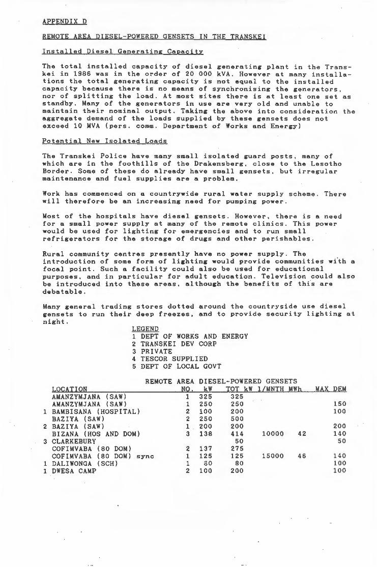
--------------~
APPENDIX D
REMOTE AREA DIESEL-POWERED GENSETS IN THE TRANSKEI
Installed Diesel Generating Capacity
The total installed capacity of diesel generating plant in the Trans kei in 1986 was in the order of 20 000 kVA. However at many installa tions the total generating capacity is not equal to the installed capacity because there is no means of synchronising the generators, nor of splitting the load. At most sites there is at least one set as standby. Many of the generators in use are very old and unable to maintain their nominal output. Taking the above into consideration the aggregate demand of the loads supplied by these gensets does not exceed 10 MVA (pers. comm. Department of Works and Energy)
Potential New Isolated Loads
The Transkei Police have many small isolated guard posts, many of which are in the foothills of the Drakensberg, close to the Lesotho Border. Some of these do already have small gensets, but irregular maintenance and fuel supplies are a problem.
Work has commenced on a countrywide rural water supply scheme. There will therefore be an increasing need for pumping power.
Most of the hospitals have diesel gensets . However, there is a need for a small power supply at many of the remote clinics. This power would be used for lighting for emergencies and to run small refrigerators for the storage of drugs and other perishables .
Rural community centres presently have no power supply. The introduction of some form of lighting would provide communities wi'th a focal point. Such a facility could also be used for educational purposes, and in particular for adult education . Television could also be introduced into these areas, although the benefits of th{s are debatable.
Many general trading stores dotted around the countryside use diesel gensets to run their deep freezes, and to provide security lighting at night.
1
2
3
1 1
LEGEND 1 DEPT OF WORKS AND ENERGY 2 TRANSKEI DEV CORP 3 PRIVATE 4 TESCOR SUPPLIED 5 DEPT OF LOCAL GOVT
REMOTE AREA DIESEL-POWERED GENSETS LOCATION NO. kW TOT kW lLMNTH MWh AMANZYMJANA (SAW) 1 325 325 AMANZYMJANA (SAW) 1 250 250 BAMBISANA (HOSPITAL) 2 100 200 BAZIYA (SAW) 2 250 500 BAZIYA (SAW) 1 200 200 BIZANA (HOS AND DOM) 3 138 414 10000 42 CLARKEBURY 50 COFIMVABA (80 DOM) 2 137 275 COFIMVABA (80 DOM) sync 1 125 125 15000 46 DALIWONGA (SCH) 1 so 80 DWESA CAMP 2 100 200
MAX DEM
150 100
200 140
50
140 100 100
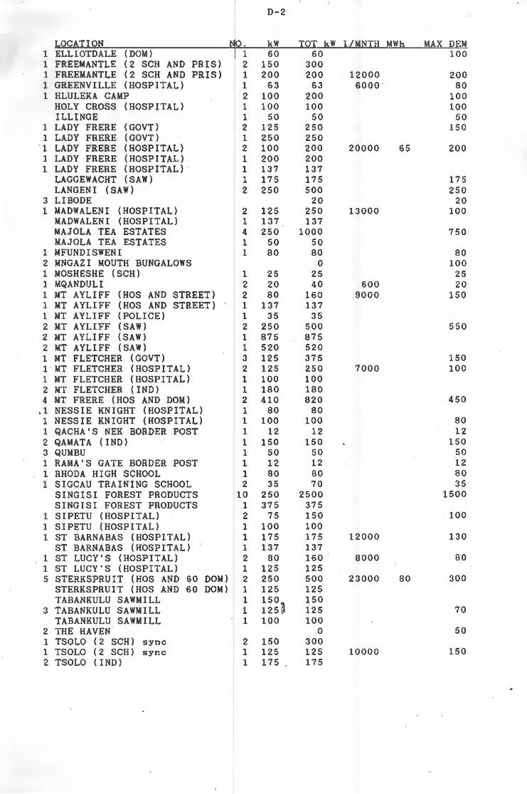
D-2
LOCATION NO. kW TOT kW lLMNTH MWh MAX DEM 1 ELLIOTDALE (DOM) 1 60 60 100 1 FREEMANTLE (2 SCH AND PRIS) 2 150 300 1 FREEMANTLE (2 SCH AND PRIS) 1 200 200 12000 200 1 GREENVILLE (HOSPITAL) 1 63 63 6ooo · 80 1 HLULEKA CAMP 2 100 200 100
HOLY CROSS (HOSPITAL) 1 100 100 100 ILLINGE 1 50 50 50
1 LADY FRERE (GOVT) 2 125 250 150 1 LADY FRERE (GOVT) 1 250 250 1 LADY FRERE (HOSPITAL) 2 100 200 20000 65 200 1 LADY FRERE (HOSPITAL) 1 200 200 1 LADY FRERE (HOSPITAL) . 1 137 137
LAGGEWACHT (SAW) 1 175 175 175 LANGEN I (SAW) 2 250 500 250
3 LIBODE 20 20 1 MADWALENI (HOSPITAL) 2 125 250 13000 100
MADWALENI (HOSPITAL) 1 137 137 MAJOLA TEA ESTATES 4 250 1000 750 MAJOLA TEA ESTATES 1 50 50
1 MFUNDISWENI 1 80 80 80 2 MNGAZI MOUTH BUNGALOWS 0 100 1 MOSHESHE (SCH) 1 25 25 25 1 MQANDULI 2 20 40 600 20 1 MT AYLIFF (HOS AND STREET) 2 80 160 9000 150 1 MT AYLIFF (HOS AND STREET) 1 137 137 1 MT AYLIFF (POLICE) 1 35 35 2 MT AYLIFF (SAW) 2 250 500 550 2 MT AYLIFF (SAW) 1 875 875 2 MT AYLIFF (SAW) 1 520 520 1 MT FLETCHER (GOVT) 3 125 375 150 1 MT FLETCHER (HOSPITAL) 2 125 250 7000 100 1 MT FLETCHER (HOSPITAL) 1 100 100 2 MT FLETCHER (IND) 1 180 180 4 MT FRERE (HOS AND DOM) 2 410 820 450
I 1 NESSIE KNIGHT (HOSPITAL) 1 80 80 1 NESSIE KNIGHT (HOSPITAL) 1 100 100 80 1 QACHA'S NEK BORDER POST 1 12 12 12 2 QAMATA (IND) 1 150 150 150 3 QUMBU 1 50 50 50 1 RAMA'S GATE BORDER POST 1 12 12 12 1 RHODA HIGH SCHOOL 1 80 80 80 1 SIGCAU TRAINING SCHOOL 2 35 70 35
SINGISI FOREST PRODUCTS 10 250 2500 1500 SINGISI FOREST PRODUCTS 1 375 375
1 SIPETU (HOSPITAL) 2 75 150 100 1 SIPETU (HOSPITAL) 1 100 100 1 ST BARNABAS (HOSPITAL) 1 175 175 12000 130
ST BARNABAS (HOSPITAL) 1 137 137 1 ST LUCY'S (HOSPITAL) 2 80 160 8000 80 1 ST LUCY'S (HOSPITAL) 1 125 125 5 STERKSPRUIT (HOS AND 60 DOM) 2 250 500 23000 80 300
STERKSPRUIT (HOS AND 60 DOM) 1 125 125 TABANKULU SAWMILL 1 150 150
3 TABANKULU SAWMILL 1 125~ 125 70 TABANKULU SAWMILL 1 100 100
2 THE HAVEN 0 50 1 TSOLO (2 SCH) sync 2 150 300 1 TSOLO (2 SCH) sync 1 125 125 10000 150 2 TSOLO (IND) 1 175 175
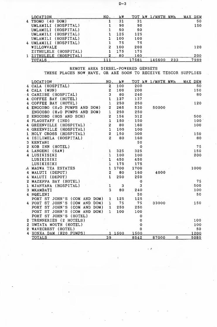
D-3
LOCATION NO. kW TOT kW lLMNTH MWh MAX DEM 4 TSOMO (40 DOM) 1 31 31 50
UMLAMILI (HOSPITAL) 1 90 90 150 UMLAMILI (HOSPITAL) 1 50 50 UMLAMILI (HOSPITAL) 1 125 125 UMLAMILI (HOSPITAL) 1 100 100
4 UMLAMILI (HOSPITAL) 1 75 75 WILLOWVALE 2 100 200 120 ZITHULELE (HOSPITAL) 1 175 175
1 ZITHULELE (HOSPITAL) 2 80 160 200 TOTALS 111 17581 145600 233 7999
REMOTE AREA DIESEL-POWERED GENSETS THESE PLACES NOW HAVE, OR ARE SOON TO RECEIVE TESCOR SUPPLIES
LOCATION NO . kW TOT kW lLMNTH MWh MAX DEM 4 CALA (HOSPITAL) 2 100 200 50 4 CALA (MUN) 2 100 200 150 4 CANZIBE (HOSPITAL) 3 80 240 80 4 COFFEE BAY (HOTEL) 1 137 137 4 COFFEE BAY (HOTEL) 1 250 250 120 4 ENGCOBO (HaO PUMPS AND DOM) 2 265 530 50000
ENGCOBO (HaO PUMPS AND DOM) 1 250 250 2 ENGCOBO (HOS AND SCH) 2 156 312 500 4 FLAGSTAFF (IND) 1 150 150 100 4 GREENVILLE (HOSPITAL) 2 80 160 100 4 GREENVILLE (HOSPITAL) 1 100 100 1 HOLY CROSS (HOSPITAL) 2 150 300 150 4 ISILIMELA (HOSPITAL) 2 80 160 80 3 KENT ANI 50 2 KOB INN (HOTEL) 0 75 4 LANGEN! (SAW) 1 325 325 150 4 LUSIKISIKI 1 100 100 200
LUSIKISIKI 1 450 450 LUSIKISIKI 1 175 175
,4 MAGWA TEA ESTATES 1 1700 1700 1000 4 MAL UTI (DEPOT) 2 80 160 4000 4 MAL UTI (DEPOT) 1 250 250 2 MAZEPPA BAY (HOTEL) 0 75 1 MJANYANA (HOSPITAL) 1 3 3 500 3 MKAMBATI 3 80 240 100 4 NQELENI 50 50
PORT ST JOHN'S (COM AND DOM) 1 125 125 4 PORT ST JOHN'S (COM AND DOM) 1 75 75 33000 150
PORT ST JOHN'S (COM AND DOM) 1 250 250 PORT ST JOHN'S (COM AND DOM) 1 100 100 PORT ST JOHN'S (HOTEL) 0
2 TRENNERIES (2 HOTELS) 0 100 2 UMTATA MOUTH (HOTEL) 0 100 2 WAVECREST (HOTEL) 0 50 4 XONXA DAM (H20 PUMPS) 1 1500 1500 1200
TOTALS 39 8542 87000 0 5080
. ·'
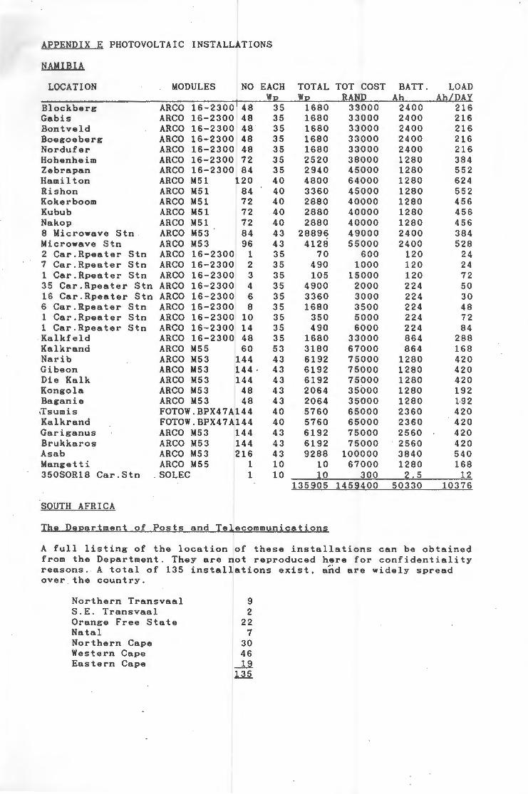
APPENDIX E PHOTOVOLTAIC INSTALLATIONS
NAMIBIA
LOCATION
Blockberg Gab is Bontveld Boegoeberg Nordufer Hohenheim Zebrapan Hamilton Rishon Koker boom Kubub Nakop 8 Microwave Stn Microwave Stn 2 Car . Rpeater Stn 7 Car.Rpeater Stn 1 Car . Rpeater Stn 35 Car.Rpeater Stn 16 Car.Rpeater Stn 6 Car.Rpeater Stn 1 Car.Rpeater Stn 1 Car.Rpeater Stn Kalkfeld Kalkrand Narib Gibeon Die Kalk Kongola Baganie .Tsumis Kalkrand Gariganus Brukkaros Asab Mangetti 350SOR18 Car.Stn
SOUTH AFRICA
MODULES NO EACH Wp
ARCO 16-2300 48 35 ARCO 16-2300 48 35 ARCO 16-2300 48 35 ARCO 16-2300 48 35 ARCO 16-2300 48 35 ARCO 16-2300 72 35 ARCO 16-2300 84 35 ARCO M51 120 40 ARCO M51 84 40 ARCO M51 72 40 ARCO M51 72 40 ARCO M51 72 40 ARCO M53 84 43 ARCO M53 96 43 ARCO 16-2300 1 35 ARCO 16-2300 2 35 ARCO 16-2300 3 35 ARCO 16-2300 4 35 ARCO 16-2300 6 35 ARCO 16-2300 8 35 ARCO 16-2300 10 35 ARCO 16-2300 14 35 ARCO 16-2300 48 35 ARCO M55 60 53 ARCO M53 144 43 ARCO M53 144· 43 ARCO M53 144 43 ARCO M53 48 43 ARCO M53 48 43 FOTOW.BPX47A144 40 FOTOW . BPX47A144 40 ARCO M53 144 43 ARCO M53 144 43 ARCO M53 216 43 ARCO M55 1 10
. SOLEC 1 10
TOTAL Wp
1680 1680 1680 1680 1680 2520 2940 4800 3360 2880 2880 2880
28896 4128
70 490 105
4900 3360 1680
350 490
1680 3180 6192 6192 6192 2064 2064 5760 5760 6192 6192 9288
10 10
135905
The Department of Posts and Telecommunications
TOT COST RAND
33000 33000 33000 33000 33000 38000 45000 64000 45000 40000 40000 40000 49000 55000
600 1000
15000 2000 3000 3500 5000 6000
33000 67000 75000 75000 75000 35000 35000 65000 65000 75000 75000
100000 67000
300 1459400
BATT. Ah
2400 2400 2400 2400 2400 1280 1280 1280 1280 1280 1280 1280 2400 2400
120 120 120 224 224 224 224 224 864 864
1280 1280 1280 1280 1280 2360 ·2360 2560 2560 3840 1280
2 . 5 50330
LOAD Ah/DAY
216 216 216 216 216 384 552 624 552 456 456 456 384 528
24 24 72 50 30 48 72 84
288 168 420 420 420 192 1·92 420 420 420 420 540 168
12 10376
A full listing of the location of these installations can be obtained from the Department . They are not reproduced here for confidentiality reasons. A total of 135 installations exist, and are widely spread over the country.
Northern Transvaal S.E. Transvaal Orange Free State Natal Northern Cape Western Cape Eastern Cape
9 2
22 7
30 46
--..il 135

E-2
All the installations are DC, the bulk of which are 24V systems with a few running at 12V, 48V and SOV.
South African Broadcasting Corporation
The SABC uses photovoltaic cells to power a number of its repeater stations. However, the engineer in charge of these systems refused to divulge any information regarding them .
Bophutatswana
The Bophutatswana security forces have installed a communications network powered almost entirely by photovoltaics . The Department of Education is also using photovoltaics to power · audio-visual equipment in remote schools .
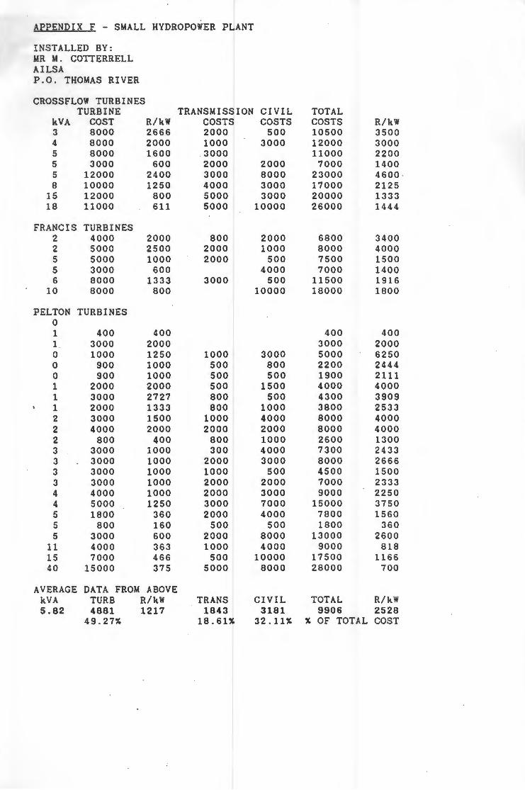
APPENDIX F - SMALL HYDROPOWER PLANT
I NSTALLED BY: MR M. COTTERRELL AILSA P . O. THOMAS RIVER
CROSSFLOW TURBINES TURBINE TRANSMISSION CIVIL TOTAL
kVA COST R/kW COSTS COSTS COSTS R/kW 3 8000 2666 2000 500 10500 3500 4 8000 2000 1000 3000 12000 3000 5 8000 1600 . 3000 11000 2200 5 3000 600 2000 2000 7000 1400 5 12000 2400 3000 8000 23000 4600 · 8 10000 1250 4000 3000 17000 2125
1 5 12000 800 5000 3000 20000 1333 18 11000 611 5000 10000 26000 1444
FRANCIS TURBINES 2 4000 2000 800 2000 6800 3400 2 5000 2500 2000 1000 8000 4000 5 5000 1000 2000 500 7500 1500 5 3000 600 4000 7000 1400 6 8000 1333 3000 500 11500 1916
10 8000 800 10000 18000 1800
PELTON TURBINES 0 1 400 400 400 400 1 3000 2000 3000 2000 0 1000 1250 1000 3000 5000 6250 0 900 1000 500 800 2200 2444 0 900 1000 500 500 1900 2111 1 2000 2000 500 1500 4000 4000 1 3000 2727 800 500 4300 3909 1 2000 1333 800 1000 3800 2533 2 3000 1500 1000 4000 8000 4000 2 4000 2000 2000 2000 8000 4000 2 800 400 800 1000 2600 1300 3 3000 1000 300 4000 7300 2433 3 3000 1000 2000 3000 8000 2666 3 3000 1000 1000 500 4500 1500 3 3000 1000 2000 2000 7000 2333 4 4000 1000 2000 3000 9000 2250 4 5000 1250 3000 7000 15000 3750 5 1800 360 2000 4000 7800 1560 5 800 160 500 500 1800 360 5 3000 600 2000 8000 13000 2600
11 4000 363 1000 4000 9000 818 15 7000 466 500 10000 17500 1166 40 15000 375 5000 8000 28000 700
AVERAGE DATA FROM ABOVE kVA TURB R/kW TRANS CIVIL TOTAL R/kW 5 . 82 4881 1217 1843 3181 9906 2528
49.27% 18.61% 32 . 11% % OF TOTAL COST
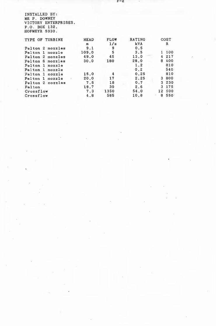
F-2
INSTALLED BY: MR P. DOWNEY VICTORY ENTERPRISES, P.O. BOX 132, HOFMEYR 5930.
TYPE OF TURBINE HEAD FLOW RATING COST m 1/s kVA R
Pelton 2 nozzles 9.1 9 0 ,5 Pelton 1 nozzle 109,0 5 3 , 5 1 100 Pelton 2 nozzles 49,0 45 13,0 4 217 Pelton 6 nozzles 30,0 180 28,0 8 400 Pelton 1 nozzle 1,2 810 Pelton 1 nozzle 0,2 540 Pelton 1 nozzle 15.0 4 0,25 810 Pelton 1 nozzle 20,0 17 2 , 25 3 800 Pelton 2 nozzles 7,5 18 0 , 7 3 230 Pelton 19,7 30 2 . 6 3 175 Crossflow 7,3 1350 54,0 12 500 Crossflow 4,8 585 10,8 8 550
REPORT NO. GEN 130
OFF-GRID SMALL POWER SUPPLY OPTIONS FOR RURAL AREAS
FINAL REPORT
A T WILLIAMS SEPTEMBER 1989