1

Occlusion Culling Algorithms: A Comprehensive Survey

Ioannis Pantazopoulos and Spyros Tzafestas

Intelligent Robotics and Automation Laboratory

Signals, Control and Robotics Division

Electrical and Computer Engineering Department

National Technical University of Athens,

Zographou, Athens, Greece

e-mail: {jpanta,tzafesta}@softlab.ece.ntua.gr

Fax: +30-1-7722490

Abstract

In this paper occlusion culling techniques appeared in the last decade are reviewed. Occlusion culling techniques are responsible for reducing the polygons rendered by the graphics hardware with the

target of achieving real time rendering. The various techniques are discussed in detail and a synopsis table with their main characteristics is given.

Keywords: Interactive time rendering, occlusion culling, spatial subdivision, aspect graph, visibility.

1. Introduction Real or interactive time rendering is a usual demand from many applications like architectural walkthroughs, medical operations, mobile robot supervision, etc. Unfortunately, although the computer power has been increased very much, the detail and complexity of the rendered models is increasing with an even faster rhythm, making hardware rendering (i.e. using local illumination models) not interactive. The rendered objects must go through a pipeline of procedures like homogeneous transformations, clipping to view frustum, lighting calculations and texture mapping before the actual rendering (i.e. scanline rasterization). There is a point that one could take advantage for many applications (like architectural walkthroughs) because usually a large fraction of the environmental objects are not visible to the observer. If one could quickly identify the objects that are hidden (occluded) he(she) could avoid all the procedures used for their rendering, thus saving time and reaching interactive rendering times. Thus, in the past decade a great variety of techniques have been proposed trying to detect non-visible objects and reject these objects from rendering (occlusion culling). Occlusion culling techniques are linked with the notion of visibility in an environment and correspond to the evolution of the first, hidden surface removal, algorithms. From the basic hidden surface removal algorithm (like painter’s algorithm with object sorting according to their distance from viewer and z-buffer), the z-buffer algorithm is today’s standard of all graphics hardware, because of its straightforward implementation and the decrease in the cost of on-board-memory. These early algorithms solve the visibility problem “locally” in opposition to occlusion culling techniques that combine information of the viewer’s position with the relative position of a number of the objects of the environment, in order to reject the rendering for complete objects or even hierarchies of the scene. A first example of occlusion culling technique is the simple view frustum culling where the environment is hierarchically divided and every node that is outside the observer’s field of view is rejected along with its descendants. In this paper, a survey of most of the occlusion culling techniques presented in the past decade is provided, revealing their advantages and disadvantages. At the beginning, the aspect graph, i.e. the structure that incorporates the whole visibility information of an environment is outlined. Theoretically, having constructed the aspect graph, it is possible to answer exactly all the information queries, but practically the cost in the construction and the demands in memory are enormous. Next, various occlusion culling techniques are analyzed classifying them in two basic categories. The paper ends with a table that codes the

2

most important characteristics of the given algorithms. One can find older surveys of occlusion culling techniques in Dorward [1994] and Cohen-Or et al. [2000].

2. Spatial Subdivision Structures As mentioned in the previous paragraph, finding whether two objects are visible to each other is one of the most time consuming but necessary procedures in occlusion culling and ray tracing techniques. In order to accelerate the procedure needed to answer such a query, there have been introduced various structures of spatial subdivision of an environment. These structures are considered as a “must” in almost all practical applications. The main issue, in the majority of these structures, is whether an object lying in two (or more) different regions should be cut in two pieces (something that is usually done offline with some extra computational cost) or duplicated in both regions (something that will lead in extra online cost but more straightforward to implement). For reasons of completeness, five of the most known spatial subdivision structures will be outlined, namely the regular grid, octrees, bsp trees, kD-trees and bounding volume hierarchies. These structures are very popular because of their relative efficiency and ease of implementation. Other more complicated and less used structures exist like irregular grids, hierarchies of sorted lists and hierarchical grids.

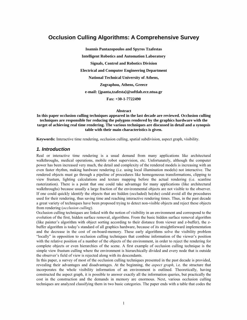
2.1. Uniform Grids The simplest spatial subdivision structure is the regular grid [Fujimoto et al. 1986]. The space is divided into cells of the same size that are axis aligned, each holding a list of the objects that lie inside them. The number and dimensions of the cells are decided in advance and thus this structure lacks any adaptability to environment. In a ray tracing procedure, when traversing the grid, one checks all the objects in the list of the current cell. The intersections, if exist, are sorted and the closest one is selected. If there is no intersection, then one moves on to the next cell and repeats the process until he(she) reaches the environment’s limits. The grid traversal in Fujimoto et al. [1986] is made possible with the use of the 3D Digital Differential Analyzer (3D-DDA) which is a variation of Bresenham’s 2D line rasterization. The differences are mostly due to the fact that the traversal needs to change in one axis only each time we proceed to the next grid node. Additionally, the starting point in grid traversal is never on the center of the cell which is taken for granted in line drawing. Usually, an environment is divided in a large number of cells and thus a great number of cells may become empty, which decreases the traversal rate.

Objects Equal-size cells

Regular Grid Octree

Scene bounding volume

Ada-ptive Cells

Figure 1. The regular grid and the octree structures.

Sometimes, the regular grid is used to identify whether a point lies inside or outside some objects of the environment. In such cases, the construction of a regular grid may be done using a procedure similar to flood-fill techniques, where a seed is put inside the environment. This is the indicated way because we expect the majority of the surfaces to be included inside a few (and most times in one) cells.

3

2.2. Octrees The octrees correspond to the hierarchical extension of the regular grids [Meagher 1982, Yamaguchi et al. 1984]. At the beginning, all the objects are bounded by an axis-aligned box. This box is recursively subdivided giving eight child-boxes where the included (and intersected) objects are stored. The subdivision continues until a maximum depth or until no object is included in the cell. Finally, every leaf of the tree (and if needed all the tree nodes as well) store a list of included objects. It is obvious that this structure is adaptive to the density and relative position of the objects in the environment in contrast to the uniform grid. Additionally, the octree traversal can be done in a more efficient (and slightly more complex) way because a number of empty regular grid cells have been turned to one octree cell. As neighbor cells, in the octree, all the cells that have a common face are taken. The intersection of an object and an axis-aligned box (which represents a cell) can be done very quickly [Greene 1994].

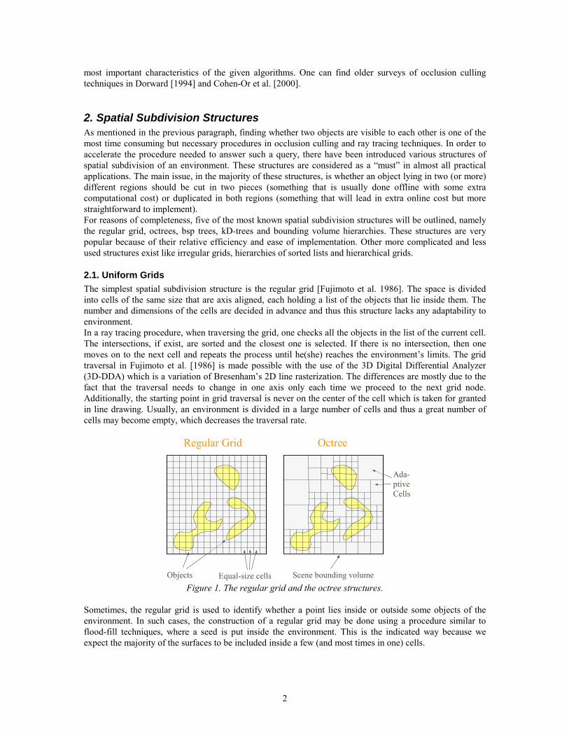
2.3. Binary Space Partitioning (bsp) Trees Bsp trees have been introduced by Fuchs [1980] and divide the environment recursively into two parts with the insertion of appropriate separating planes. Usually, for polygonal scenes, the separating planes are chosen to coincide with one of the input polygons. All the coincident, with the plane, polygons are inserted into the list of the created node while the others are classified as front or back. If the plane splits a polygon then the created parts (two convex polygons for a convex split polygon) are also classified as front or back. The existence of split polygons means that the number of polygons from a level to the level of the tree is not necessarily decreased. Nevertheless, the creation of an optimized bsp tree (under the notion of a balanced tree with the least number of total polygons) is an NP-complete problem. Practically, the construction of a bsp tree is based on a number of heuristics.

1

2

3 1

2

3

4

1

2

3 1

2

3 1

2

3

4

1

2

3

4

Bsp-Tree kD-Tree

Partition PlanesPartition Planes Figure 2. The bsp tree and kD tree structures.

2.4. kD-trees kD-trees are a specialization of bsp trees where the partitioning planes are aligned with the three base planes xy, xz, yz [Bentley 1975]. This means that there is a simplification in choosing the appropriate partitioning plane where one has to choose one of the three possible ones and the height (split abscissa) of the partition. For example, the plane z=a is a partitioning plane, parallel to xy plane, with split abscissa equal to a.

2.5. Bounding Volume Hierarchies The bounding volume hierarchy structure is more closely adapted to the shape of the objects than the previous four structures presented [Goldsmith et al. 1987]. The objects are put at the correct level of the constructed tree, depending on their size and semantics. For example, the bounding volume of a desk is considered as a child volume of the room volume where it is, while it can a parent volume to those of its drawers. For the bounding volume shape can be chosen any appropriate closed surface like spheres, axis aligned or arbitrarily oriented boxes etc. Usually, the boxes (parallelepipeds) are the most common ones,

4

with the arbitrarily oriented ones fitting more tightly to the object shape while having more complexity in handling them (for example, less efficient intersection algorithms). In general, bounding volumes can be used separately or with another spatial subdivision structure to enhance even more visibility queries.

3. Preliminaries The main problem solved by the occlusion culling techniques is identifying the visible objects from the viewer’s position. In general, the input of occlusion culling techniques is the whole environment and the viewer’s position, and their output is a list of (exactly, potentially or approximately) visible objects. Theoretically speaking, we would like to find the set S={P1,...,Pn} of all the objects that are visible from a specific viewer position (the “position” here includes eye position, view direction and field of view). An object is considered visible if there exists a point on its surface that can be connected with the eye position without intersecting any other object of the environment while this point is inside the viewer’s view frustum. We give here some formal definitions after [Saona Vazquez et al. 1999]: Definition 1. The shadow of a set A⊆ Rn from a light point p, is the set:

{ }AqApqRqApS n ∉∧∅≠∈= �|),( where pq is the segment connecting points p and q. Definition 2. The shadow of a set A⊆ Rn from a light surface P⊆ Rn, is the set:

{ } ��Pp

n ApSAqApqPpRqAPS∈

=∉∧∅≠∈∀∈= ),(:|),(

These definitions give a theoretical basis for finding out whether some objects lie in the shadow of others or more generally whether two objects “can see each other” in the given environment. This latter query is the most fundamental one in occlusion culling maters as in ray tracing algorithms and, for large environments, a very time consuming one. In general, occlusion culling techniques have various characteristics involving the ease of implementation or rendering speed. A basic “measurement unit” of these characteristics, is the fraction of overestimation of the visible objects. The less this fraction is, the more “accurate” will the technique be (with the aspect graph being, in a general environment, the only technique of zero overestimation). When there is an overestimation of the visible objects then the list of these objects is called “Potentially Visible Set” or PVS in short. The fact that one technique is more “accurate” than another, does not guarantee that it is going to be faster though, because it is the case that the time consumed to reject some non visible objects is greater than the time needed to directly render them without a second thought. It is obvious here that there exists a trade off between the “accuracy” and the rendering speed and the actual best time-response point depends on both the complexity of the environment and the characteristics of the graphics hardware. An important characteristic of an occlusion culling technique is whether it can combine two or more objects in order to classify others being hidden from the former combination. This is noted as “occluder fusion” and in most cases leads to an increase of the “accuracy” of the technique. A third characteristic of a technique is whether it can take into account results from previous frames (temporal coherence), thus reducing the cost of finding the whole list of visible object to a clever update of this list. Another characteristic is whether the calculations of a technique are done in 3d space, involving computational geometry techniques, or in image space, involving some basic image processing (and in a few cases both spaces are used to cull objects). The calculations in image space, although simpler because of the reduced space dimension, can sometimes lead to visual artifacts, thus, some extra care is needed in designing such algorithms. Finally, the way in which certain objects are selected to play the role of occluders, is a critical point of these techniques. Usually, this role is played by large objects, close to the viewer, thus having a great chance of hiding other objects lying behind them. A characteristic parameter of this occlusion ability of a certain object is the solid angle criterion (where the eye position is also taken into account). An approximation of this criterion for polygonal occluders has been given by Coorg et al. [1996]:

Solid angle criterion : ( ) 2DVNA ⋅⋅−

5

where A is the surface of the occluder, N is the normal vector to the polygonal occluder, D is the vector connecting the viewer with the occluder’s center and V is the view direction. The aspect graph will be presented in the next section as it involves the main theory behind occlusion culling techniques. The occlusion culling techniques are classified into two basic categories, those that find the visible objects for every new viewer position (visibility from a point) and those that keep the same visible object list for more than one position (visibility from a region). As we will see, the characteristics of these classes are quite different to justify this separation.

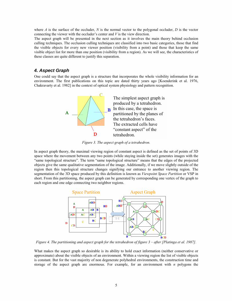
4. Aspect Graph One could say that the aspect graph is a structure that incorporates the whole visibility information for an environment. The first publications on this topic are dated thirty years ago [Koenderink et al. 1976, Chakravarty et al. 1982] in the context of optical system physiology and pattern recognition.

A

D

B

C

A

D

B

C

A

D

B

CThe simplest aspect graph is produced by a tetrahedron. In this case, the space is partitioned by the planes of the tetrahedron’s faces. The extracted cells have “constant aspect” of the tetrahedron.

Figure 3. The aspect graph of a tetrahedron.

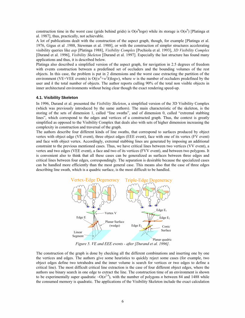
In aspect graph theory, the maximal viewing region of constant aspect is defined as the set of points of 3D space where the movement between any two points (while staying inside the set) generates images with the “same topological structure”. The term “same topological structure” means that the edges of the projected objects give the same qualitative segmentation of the image. Additionally, if we move slightly outside of the region then this topological structure changes signifying our entrance to another viewing region. The segmentation of the 3D space produced by this definition is known as Viewpoint Space Partition or VSP in short. From this partitioning, the aspect graph can be generated by corresponding one vertex of the graph to each region and one edge connecting two neighbor regions.

A A BA D

A B DB

BD

A D C A C A B CBC

BCDC D

C D

A

AC

AD

ADC

D BD

ABD

AB

ABC

B

BCC

CD

BC D

A A BA D

A B DB

BD

A D C A C A B CBC

BCDC D

C D

A A BA D

A B DB

BD

A D C A C A B CBC

BCDC D

C D

A

AC

AD

ADC

D BD

ABD

AB

ABC

B

BCC

CD

BC D

A

AC

AD

ADC

D BD

ABD

AB

ABC

B

BCC

CD

BC D

1-1

Space Partition Aspect Graph

Figure 4. The partitioning and aspect graph for the tetrahedron of figure 3 – after [Platinga et al. 1987].

What makes the aspect graph so desirable is its ability to hold exact information (neither conservative or approximate) about the visible objects of an environment. Within a viewing region the list of visible objects is constant. But for the vast majority of non degenerate polyhedral environments, the construction time and storage of the aspect graph are enormous. For example, for an environment with n polygons the

6

construction time in the worst case (grids behind grids) is O(n9logn) while its storage is O(n9) [Platinga et al. 1987], thus, practically, not achievable. A lot of publications dealt with the construction of the aspect graph, though, for example [Platinga et al. 1976, Gigus et al .1988, Stewman et al. 1988], or with the construction of simpler structures accelerating visibility queries like asp [Platinga 1988], Visibility Complex [Pochiola et al. 1993], 3D Visibility Complex [Durand et al. 1996], Visibility Skeleton [Durand et al. 1997]. Especially the last structure has found many applications and thus, it is described below. Platinga also described a simplified version of the aspect graph, for navigation in 2.5 degrees of freedom with events construction between a predefined set of occluders and the bounding volumes of the rest objects. In this case, the problem is put in 2 dimensions and the worst case extracting the partition of the environment (VE+VEE events) is O((w4+w3k)logw), where w is the number of occluders predefined by the user and k the total number of objects. The author reports culling 90% of the total non visible objects in inner architectural environments without being clear though the exact rendering speed-up.

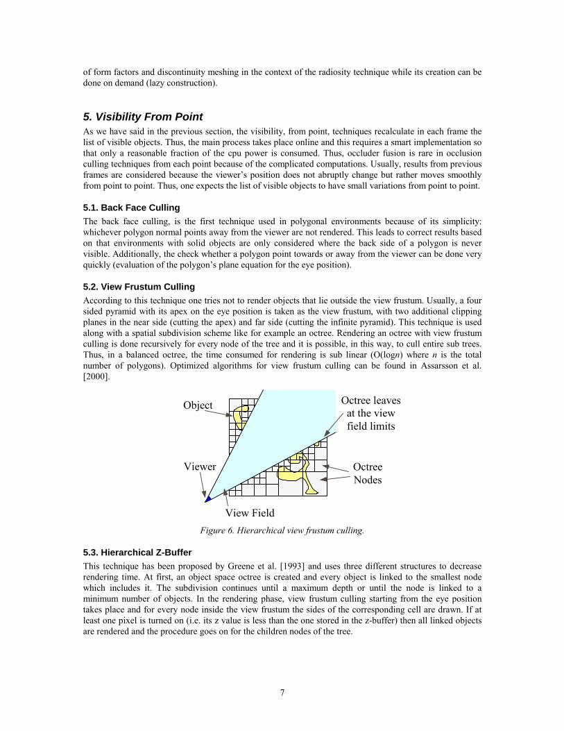
4.1. Visibility Skeleton In 1996, Durand et al. presented the Visibility Skeleton, a simplified version of the 3D Visibility Complex (which was previously introduced by the same authors). The main characteristic of the skeleton, is the storing of the sets of dimension 1, called “line swaths”, and of dimension 0, called “extremal stabbing lines”, which correspond to the edges and vertices of a constructed graph. Thus, the context is greatly simplified as opposed to the Visibility Complex that deals also with sets of higher dimension increasing the complexity in construction and traversal of the graph. The authors describe four different kinds of line swaths, that correspond to surfaces produced by object vertex with object edge (VE event), three object edges (EEE event), face with one of its vertex (FV event) and face with object vertex. Accordingly, extremal stabbing lines are generated by imposing an additional constraint to the previous mentioned cases. Thus, we have critical lines between two vertices (VV event), a vertex and two edges (VEE event), a face and two of its vertices (FVV event), and between two polygons. It is convenient also to think that all these cases can be generalized as surfaces between three edges and critical lines between four edges, correspondingly. The separation is desirable because the specialized cases can be handled more efficiently than the most general case. This means also that the case of three edges describing line swath, which is a quadric surface, is the most difficult to be handled.

Vertex-Edge Degeneracy Triple-Edge Degeneracy

Vertex V Edge E

Planar Surface(wedge)

Linear Segment

Edge E1

Edge E2

Edge E3 Conic Surface

Planar quadric Figure 5. VE and EEE events - after [Durand et al. 1996].

The construction of the graph is done by checking all the different combinations and inserting one by one the vertices and edges. The authors give some heuristics to quickly reject some cases (for example, two object edges define two tetrahedra and the inner volume is search for vertices or two edges to define a critical line). The most difficult critical line extraction is the case of four different object edges, where the authors use binary search in one edge to extract the line. The construction time of an environment is shown to be experimentally super quadratic ~O(n2.4), with the number of polygons n between 84 and 1488 while the consumed memory is quadratic. The applications of the Visibility Skeleton include the exact calculation

7

of form factors and discontinuity meshing in the context of the radiosity technique while its creation can be done on demand (lazy construction).

5. Visibility From Point As we have said in the previous section, the visibility, from point, techniques recalculate in each frame the list of visible objects. Thus, the main process takes place online and this requires a smart implementation so that only a reasonable fraction of the cpu power is consumed. Thus, occluder fusion is rare in occlusion culling techniques from each point because of the complicated computations. Usually, results from previous frames are considered because the viewer’s position does not abruptly change but rather moves smoothly from point to point. Thus, one expects the list of visible objects to have small variations from point to point.

5.1. Back Face Culling The back face culling, is the first technique used in polygonal environments because of its simplicity: whichever polygon normal points away from the viewer are not rendered. This leads to correct results based on that environments with solid objects are only considered where the back side of a polygon is never visible. Additionally, the check whether a polygon point towards or away from the viewer can be done very quickly (evaluation of the polygon’s plane equation for the eye position).

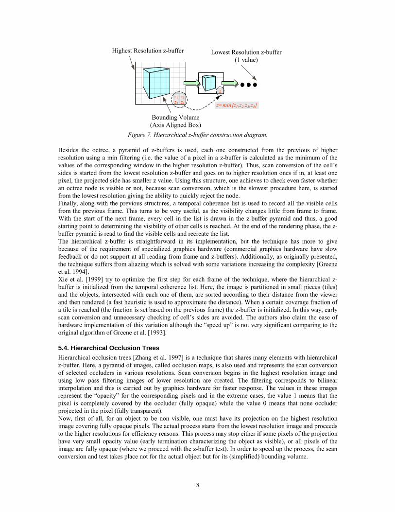
5.2. View Frustum Culling According to this technique one tries not to render objects that lie outside the view frustum. Usually, a four sided pyramid with its apex on the eye position is taken as the view frustum, with two additional clipping planes in the near side (cutting the apex) and far side (cutting the infinite pyramid). This technique is used along with a spatial subdivision scheme like for example an octree. Rendering an octree with view frustum culling is done recursively for every node of the tree and it is possible, in this way, to cull entire sub trees. Thus, in a balanced octree, the time consumed for rendering is sub linear (O(logn) where n is the total number of polygons). Optimized algorithms for view frustum culling can be found in Assarsson et al. [2000].

View Field

Viewer

Object

Octree Nodes

Octree leaves at the view field limits

Figure 6. Hierarchical view frustum culling.

5.3. Hierarchical Z-Buffer This technique has been proposed by Greene et al. [1993] and uses three different structures to decrease rendering time. At first, an object space octree is created and every object is linked to the smallest node which includes it. The subdivision continues until a maximum depth or until the node is linked to a minimum number of objects. In the rendering phase, view frustum culling starting from the eye position takes place and for every node inside the view frustum the sides of the corresponding cell are drawn. If at least one pixel is turned on (i.e. its z value is less than the one stored in the z-buffer) then all linked objects are rendered and the procedure goes on for the children nodes of the tree.

8

z

z4z3

z2z1

z=min{z1,z2,z3,z4}

Highest Resolution z-buffer

Bounding Volume (Axis Aligned Box)

Lowest Resolution z-buffer (1 value)

Figure 7. Hierarchical z-buffer construction diagram.

Besides the octree, a pyramid of z-buffers is used, each one constructed from the previous of higher resolution using a min filtering (i.e. the value of a pixel in a z-buffer is calculated as the minimum of the values of the corresponding window in the higher resolution z-buffer). Thus, scan conversion of the cell’s sides is started from the lowest resolution z-buffer and goes on to higher resolution ones if in, at least one pixel, the projected side has smaller z value. Using this structure, one achieves to check even faster whether an octree node is visible or not, because scan conversion, which is the slowest procedure here, is started from the lowest resolution giving the ability to quickly reject the node. Finally, along with the previous structures, a temporal coherence list is used to record all the visible cells from the previous frame. This turns to be very useful, as the visibility changes little from frame to frame. With the start of the next frame, every cell in the list is drawn in the z-buffer pyramid and thus, a good starting point to determining the visibility of other cells is reached. At the end of the rendering phase, the z-buffer pyramid is read to find the visible cells and recreate the list. The hierarchical z-buffer is straightforward in its implementation, but the technique has more to give because of the requirement of specialized graphics hardware (commercial graphics hardware have slow feedback or do not support at all reading from frame and z-buffers). Additionally, as originally presented, the technique suffers from aliazing which is solved with some variations increasing the complexity [Greene et al. 1994]. Xie et al. [1999] try to optimize the first step for each frame of the technique, where the hierarchical z-buffer is initialized from the temporal coherence list. Here, the image is partitioned in small pieces (tiles) and the objects, intersected with each one of them, are sorted according to their distance from the viewer and then rendered (a fast heuristic is used to approximate the distance). When a certain coverage fraction of a tile is reached (the fraction is set based on the previous frame) the z-buffer is initialized. In this way, early scan conversion and unnecessary checking of cell’s sides are avoided. The authors also claim the ease of hardware implementation of this variation although the “speed up” is not very significant comparing to the original algorithm of Greene et al. [1993].

5.4. Hierarchical Occlusion Trees Hierarchical occlusion trees [Zhang et al. 1997] is a technique that shares many elements with hierarchical z-buffer. Here, a pyramid of images, called occlusion maps, is also used and represents the scan conversion of selected occluders in various resolutions. Scan conversion begins in the highest resolution image and using low pass filtering images of lower resolution are created. The filtering corresponds to bilinear interpolation and this is carried out by graphics hardware for faster response. The values in these images represent the “opacity” for the corresponding pixels and in the extreme cases, the value 1 means that the pixel is completely covered by the occluder (fully opaque) while the value 0 means that none occluder projected in the pixel (fully transparent). Now, first of all, for an object to be non visible, one must have its projection on the highest resolution image covering fully opaque pixels. The actual process starts from the lowest resolution image and proceeds to the higher resolutions for efficiency reasons. This process may stop either if some pixels of the projection have very small opacity value (early termination characterizing the object as visible), or all pixels of the image are fully opaque (where we proceed with the z-buffer test). In order to speed up the process, the scan conversion and test takes place not for the actual object but for its (simplified) bounding volume.

9

Second, if an object passes the first test it must be also in a depth greater than that of the occluders. Here, a z-buffer is used where the more distant vertex of the bounding volume of the occluders is compared with the closest vertex of the bounding volume of the occludee. For an alternative, the use of a separating plane in front of the occluders is proposed and the search for occludees is reduced to the opposite side of the plane is proposed (simple but very conservative solution). Thus, in general, the technique is separated in a preprocessing phase where an occluder database is built up and a navigation phase where selection of “active” occluders, construction of occlusion maps and culling of bounding volumes of the objects takes place. The occluders, inserted in the database, are selected by their size, and the authors have also used simplification techniques for the stored polygonal occluders (something that leads to visual artifacts). In navigation, the occluders are selected from the database by their size and distance from the viewer being inside the view frustum, while some heuristics are described for best adaptation of the number of used occluders. The technique has been tested in a city model (312,524 polygons), submarine model (632,252 polygons) and a dynamic environment (986,000 polygons) where the average culling varied from 80% to 95%.

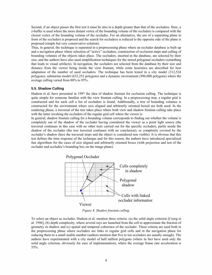
5.5. Shadow Culling Hudson et al. have presented in 1997 the idea of shadow frustum for occlusion culling. The technique is quite simple for someone familiar with the view frustum culling. In a preprocessing step, a regular grid is constructed and for each cell a list of occluders is found. Additionally, a tree of bounding volumes is constructed for the environment where axis aligned and arbitrarily oriented boxed are both used. In the rendering phase, a traversal of the tree takes place where both view and shadow frustum culling take place with the latter invoking the occluders of the regular grid cell where the viewer is. In general, shadow frustum culling for a bounding volume corresponds to finding out whether the volume is completely out of the shadow of the occluder having considered the viewer as a point light source (the traversal continues in this case with no other tests carried out for the specific occluder), partly inside the shadow of the occluder (the tree traversal continues with no conclusion), or completely covered by the occluder’s shadow (here the traversal stops and the object is considered non visible). It is obvious that this test defines the time response of the technique and for this reason, the authors have introduced specialized fast algorithms for the cases of axis aligned and arbitrarily oriented boxes (with projection and test of the occluder and occludee’s bounding box on the image plane).

Polygonal Occluder

Viewer

Cells completely in shadow

Polygonal shadow

Cells with linked occluder information

Figure 8. Shadow frustum culling.

To select an object as occluder, Hudson et al. mention three criteria: (a) the solid angle criterion [Coorg et al. 1996], (b) depth complexity, where several rays are launched from the cell to approximate the fraction of geometry in shadow and (c) spatial and temporal coherence of the occluder. These criteria are used both in the preprocessing phase where occluders are links to regular grid cells and in the navigation phase for reducing them to a small usable number (authors mention that five to ten occluders are usually enough). The authors have experimented with a city model of half million polygons (where in fact have used only the solid angle criterion, obviously for ease of implementation), where the average frame rate acceleration is 55%.

10

5.6. Supporting and Separating Planes Coorg et al. [1997] have used the technique of supporting and separating planes in order to verify whether an axis aligned box is in the shadow of another convex polygon. Even more, taking into account some of the supporting and separating planes created by occluder edges and occludee vertices (and vice versa), they manage to fuse occluders if the union of their shadows corresponds to a new (increased) convex occluder. From this point of view, the authors describe a novel algorithm to find the supporting and separating planes between a convex occluder and an axis aligned box (this process degenerates to finding tangents to the corresponding projected entities in two dimensions). Optimization of the particular algorithm technique is necessary as it is the bottleneck of the technique, and pre-constructed look up tables are used. In the navigation phase, a kD-tree, subdividing the environment, is traversed and we test for each node whether it is in the shadow of an occluder. If it is partly in the shadow, then the traversal continues for the children nodes, otherwise either we stop traversal or the node is considered fully visible and all linked objects are immediately rendered. The occluders, used for the culling process, are small in number and are selected in a preprocessing phase based on the solid angle criterion for several points in the kD tree cell they afterwards linked. Additionally, lists of possible occluders are taken into account for very small and detailed objects possibly reducing even more the rendered objects. Finally, one may say that supporting and separating planes calculated from previous frames are reused because the used set of occluders changes little over viewer’s movement (temporal coherence). The authors have presented simulations of the city models and the Soda Hall model. The rendered polygons represent only 5.6% and 2.6% of the total polygons for the models, while view frustum culling rendered 36.9% and 19.7% correspondingly. Nevertheless, the cpu usage increases with the speed of the observer. This is because the greater the speed of the viewer, the less results can be used from previous frames, and thus supporting and separating planes have to be recalculated.

5.7. Occlusion Trees Bittner et al. [1998] have presented occlusion trees for online visibility determination, structures that have great similarity with shadow volume trees [Chin et al. 1990]. In the preprocessing phase, possible occluders are marked while at the same time a kD tree of the scene is constructed. The authors deal mainly with architectural models and thus, the occluders are usually represented by the building walls. The occluders are selected online from those marked occluders within a certain range from the viewer based on the solid angle criterion. Selected occluders are sorted according to their distance from the viewer in order to construct the occlusion bsp tree in the same way a shadow volume bsp tree is constructed. From now on, any convex polygon (and again, for efficiency reasons, the faces of a kD tree cell are tested and not the actual objects) can be conservatively classified according to the occlusion tree whether it is invisible, partly or fully visible (the tree traversal goes on accordingly). The actual process, i.e. the sorting using the bsp tree, requires a final test for the polygon fragment reaching a leaf that is occluded (in-leaf), in order to find the relative position of the fragment to the occluder’s plane. Even more, the authors use some heuristics for faster tree traversal (for example, if a kD tree node has only a few included objects then it is rendered without any test) and previous results (temporal coherence) with marking of tree nodes that no test is needed to be carried out in the next frame. Additionally, they give a modified version of the occlusion tree, where in the construction phase, edges of occluders, split along their direction, are marked in order to reduce the total number of nodes in the bsp tree. In the modified version, the axis aligned cells of the kD tree are tested without split against the nodes of the bsp tree, thus loosing the ability to perform occluder fusion. The authors have experimented with architectural buildings, where acceleration of 2.5 to 3.75 times against view frustum culling is shown.

5.8. Linearized Aspect Graph Coorg et al. [1996] presented a kind of linearized version of the aspect graph structure. They used only VE events between vertices and edges of convex polyhedra and specifying visibility by the following conservative rule: a polygon is invisible if all its vertices are hidden by a convex polyhedron. Even such a simplification (no EEE events are taken into account) leads to an enormous partition of the environment. The authors take the idea one step further by considering only the planes defining the cell where the viewer

11

is (relevant planes), thus keeping only a small fraction O(n2) of the total planes. These planes are the supporting and separating planes between some polyhedral occluders and occludees. Thus, should the viewer pass to another cell, he will have to cross one of the relevant planes. In this occasion, new defining planes are calculated using the winged edge structure and the list of visible objects is refreshed. In a way, this technique shares some characteristics from region occlusion culling techniques but the visible objects are determined online. The calculation of the defining planes is carried out with an additional spatial subdivision structure, like an octree. In this case, a traversal and characterization of the nodes of the tree to non visible, partly or completely visible in respect to a certain occluder is used to extract the supporting and separating planes. Additionally, the authors give basic commands for keeping track of the planes (insertion, deletion and finding of crossed planes while moving) and analyze advantages and disadvantages of spatial structures used for this (a list of planes inside a sphere centered at the viewer, an octree sorting the planes). Occluders are selected dynamically at the navigation phase based on the size of their projection on the image. In simulations with architectural models, the authors report occlusion culling of 68% (Soda Hall model) and 36% (city model) while the average fraction of visible objects was between 5% and 10%.

5.9. Lod Occluders A novel idea was that of Andujar et al. [1999] where occluders are produced in various resolutions, based on some object models. The main idea is to concatenate several parallelepiped occluders of high resolution in order to create a few lower resolution occluders with almost the same “visibility properties” possibly covering some chasms and holes. This means that we have approximate visibility but the authors claim here that the error in the image is small and upper bounded. In such a technique, it is important the way occluders are extracted based on a model. The strategy here is to build a maximal division octree where each node is characterized as white (i.e. transparent), black (i.e. opaque) or gray with additional separation between boundary and inner nodes. This in this step (aggregation step), the model has been simplified and the rest of the work can be done with faces of the tree nodes. The second step (convex extraction) is the hardest one and involves the solution of the maximal containment problem based on some heuristics. Here, parallelepipeds starting from random black leaves are dilated along the principal axis while kept inside black nodes of the tree. Additionally, these parallelepipeds can be extended to reach boundary nodes thus removing any concavities and holes since the shadow produced by a point light source viewer is - most times - conservatively altered. Andujar et al. go one step further by extracting sets of lower resolution from these parallelepipeds where occluders very close to each other are concatenated. Using simple error metrics for the produced image, the occluders are selected one by one in the navigation phase starting with the ones giving the smaller distortion. Afterwards, the objects are classified as visible or non visible depending on their relative position to the occluders and the viewer. The occluder extraction is tested on a model of cathedral with success while in a city model (~183,000 polygons) an average 40% more culling than that of the separate occluders (without concatenation) is reported. In a later publication [Andujar et al. 2000], the authors use these results (and of Visibility Octree structure of the same authors) to define Hardly Visible Sets. These sets give in fact a sorting of partly visible objects in various classes depending on two error metrics (ea error metric: relative to the total number of visible pixels of the object, et error metric: relative to the maximum opaque part of the object). At the same time, heuristics (like projection size, centered projection, speed of movement and importance of the object) are given for the selection of the detail level of the rendered objects which are extracted from the hardly visible sets. The authors give two different strategies for the creation of the sets following the one where pre-selected occluders are dilated and unite, giving approximate visibility.

5.10. OpenGL Assisted Culling Bartz et al. [1999] use the graphics hardware to achieve occlusion culling with high frame rates. Their technique is used on slopy n-ary space partitioning trees in conjunction with view frustum culling. The bounding volumes are found for the objects in the environment and a hierarchy is constructed where the nodes (i.e. the bounding volume shapes) may overlap each other in contrast with the usual approaches. In both view frustum culling and occlusion culling the frame buffer of standard OpenGL hardware is read.

12

The idea is quite simple: a front to back rendering is performed, for all nodes inside the view frustum, for the bounding volumes using the stencil buffer. The stencil buffer is read after the rendering of a volume and thus whether the node is visible or not is checked. The transfer of the information from the graphics hardware to the cpu is the slowest part of the algorithm and in practice, only a few pixels are read (and the technique is turned to a non conservative one). Even more, the number of pixels written by the bounding volume represents an estimation of the object’s contribution. When this number is small enough the bounded objects are not rendered at all (adaptive culling). In addition, occlusion culling process takes place for only a fraction of the rendering time of the previous frame. After that, nodes of the tree not yet tested for occlusion are sent directly for rendering. The technique is tested in various environments with an average culling of 90% while the acceleration varies from 4 to 12 times (which depends heavily on the graphics hardware). The authors extend also some ideas of Scott et al. [1998] proposing hardware modifications for fast transfer of information specific to the contribution of the rendered objects to the frame buffer.

5.11. Prioritized Layered Projection (PLP) Klosowski et al. [1999] do not try to directly perform occlusion culling, but sort the polygons of the environment in such a way so as by rendering a fraction of them from any position, the drawn image will correspond very much to the actual visible objects. Thus, in a preprocessing step an octree of the environment is constructed and a Delaunay triangulation is carried out on cells’ centers. The environment is then partitioned in new tetrahedral cells with additional neighborhood information and density (or “solidity” as posed) of the included objects. The latter characteristic is also very important in the cell traversal. At the beginning of the rendering phase, the tetrahedra in front of the viewer are inserted into a queue. This queue sorts the tetrahedra according to their solidity. Thus, the tetrahedron with the lowest solidity is selected for rendering and all neighbor cells are put into the queue. The solidity value of the inserted cells is defined by the one which is rendered and its relative position to the viewer (for example, if the center of the tetrahedron is not visible through the face common with the rendered neighbor, the solidity is increased - non star shaped penalty - and in this way the front to back rendering is in general maintained. When a certain number (budget) of rendered objects is reached the rendering phase terminates. Obviously, a basic application of this technique is in environments where interactive time is the first requirement even with the cost of lower image quality. The authors experiment with a city model (~500,000 triangles) and a car model (~810,000 triangles) where with a 10% budget, successful renderings of 90% and 76% correspondingly of the visible objects are carried out.

5.12. Conservative Prioritized Layered Projection (cPLP) In a later trial, Klosowski et al. [2001] extend the PLP technique in order to become a conservative one. The first step of the new algorithm cPLP is a rendering on a budget step as in the original PLP, although here the leaf nodes of the octree are used instead of the tetrahedra produced by the Delaunay triangulation. The algorithm then takes on from the point which PLP is terminated. Here, the bounding volumes in the priority queue are projected on the image plane and we find which of them are visible and which are not. For those which are visible, the included objects are rendered and afterwards the neighbor cells, not yet visited, are put in the queue. This process is repeated until the queue is empty or none of the projected volumes onto the image is visible. The query whether a volume is visible or not is the most critical in the algorithm and the authors analyze various hardware architectures for its answer (special occlusion test supported by HP fx6 hardware, item buffer for reading of the color buffer after assignment of discrete colors to each one of the volumes, histogram extension for minimizing the information transferred between the hardware and cpu). They recommend some software enhancements, like tiling for partitioning the image into smaller pieces and querying for occlusion each one separately and an extension to histogram function of OpenGL hardware for greater efficiency. The authors give comparative tests for various versions of the cPLP algorithm in architectural drawings with more than 1 million triangles, where it is obvious the high dependence of the algorithm with the platform used (for example, the item buffer cPLP method is the best in Octane and Onyx platforms but disappointing in HP Kayak). The frame rate depends also on the budget of the PLP sub-technique (it varies from 9 to 23 fps for the best architecture) but without being clear an optimum way of selecting it. In a

13

similar environment, the authors report a speed up of 3 times as opposed to hierarchical view frustum culling based on the comparing counts in the z-buffer.

5.13. Lazy Occlusion Grid Similarly to the tiled architecture technique of Xie et al. [1999] and Hey et al. [2001] presented a technique based on a 2D low resolution grid, where the object bounding volumes are drawn. One could say that the technique is similar in logic to the hierarchical z-buffer replacing the z-buffer pyramid with a single low resolution image. In the first of the two variations presented, an occlusion buffer is created where each value represents whether the corresponding image cell is occluded or not while in the second variation, a z-buffer is used where each value represents the maximum distance for all cell pixels. Additionally, for each cell, there is a flag that states whether the cell value is outdated or not, and in conjunction with the rendering algorithm justifies the “lazy” characteristic of the technique. In general, the rendering phase has the following steps: the projection of a bounding volume on the low resolution image is found and all the whole “inner” cells of the projection are search one by one whether they are occluded or not. The same holds for the “boundary” cells of the projection but there the pixels of the cell are searched. If a cell has outdated value then its value is updated from the standard resolution z-buffer (i.e. on demand update). At the first unoccluded cell, the process stops and all objects of the bounding volume are rendered while the rest cells of the projection are marked with an outdated flag. For the faster possible results, in the z-buffer variation, a front to back rendering is followed while in the occlusion buffer variation, a special front to back rendering order is given where volumes that can not be sorted according their distance from viewer, are tested before rendered (two different lists are used here). The authors show how an implementation could be supported by various hardware functions. A disadvantage is that, today, most occlusion queries are not supported by standard hardware and the existence of a software renderer in addition to reading z-buffer leads to reduced performance. For comparison, in some test environments (a forest of 1.7 million polygons, a city of 34 million polygons) about half of the total rendering time comes from reading hardware frame buffers and things are much worse when the “lazy” approach is not employed. The acceleration varies between 2 and 40 times in comparison to view frustum culling. Finally, we should say that the optimum cell size is found experimentally by checking the rendering time for various typical scenes.

6. Visibility From Region In contrast to the point visibility techniques, occlusion culling techniques with visibility from region use the potentially visible set for many sequential positions of the viewer. In general, the environment is partitioned to many cell (according to a spatial subdivision structure) and objects that are visible for at least one position in the cell are offline calculated and stored. Thus, the basic procedure does not take place in parallel with rendering, giving the ability to use more exhausting and complicated algorithms. Nevertheless, the lists of visible objects, created offline for each cell, can be huge and this is a disadvantage for most techniques that can not deal with it. Of course, the benefit using a region occlusion culling technique is the minor cpu usage in the navigation phase.

6.1. Portals The notion of portals was first presented by Airey [1990]. The name “portals” characterizes some of the holes between opaque objects. For example, one could characterize as portals, the windows and doors in buildings (indoor scenes). In the general case, in order to solve the visibility problem, the portals are viewed as surface lights and all objects in front of them cast shadows (creating shadow volumes). Then the visibility problem is transformed to finding all objects being in shadow and consequently not visible through the corresponding portal. Thus, in a preprocessing phase, every object that is visible through a portal, are put into a list linked to the portal. At the navigation phase, the viewer is always inside a room (more generally in a cell) that is connected to neighbor rooms via portals. For every visible portal, all linked objects are rendered. In a more recent publication, portals have been used in indoor building scenes with axis aligned rooms [Teller et al. 1993]. In this case, the axis aligned polygons are used for the partition of the environment into cells that connected to each other by windows and doors (i.e. portals). The walls are classified, in respect to

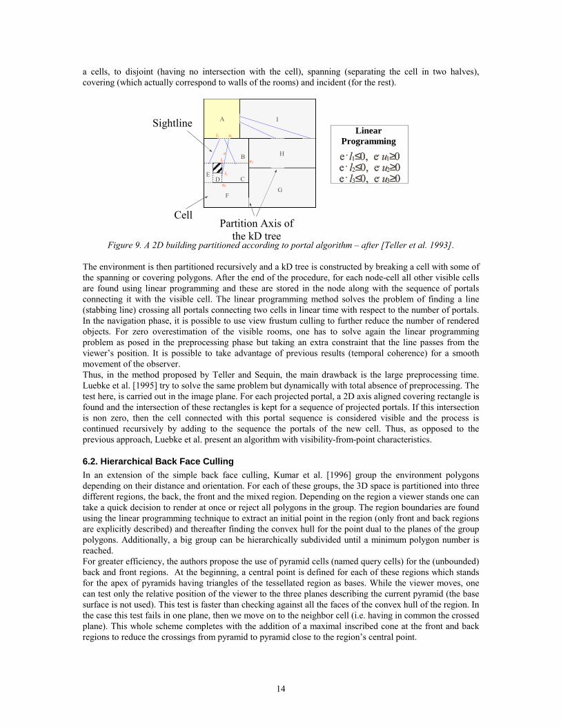
14

a cells, to disjoint (having no intersection with the cell), spanning (separating the cell in two halves), covering (which actually correspond to walls of the rooms) and incident (for the rest).

Α

Β

CD E

FG

H

I

l 1 u1

l 2 u2

l 3u 3

e e . l1≤ 0, e . u1≥ 0 e . l2≤ 0, e . u2≥ 0 e . l3≤ 0, e . u3≥ 0

Α

Β

CD E

FG

H

I

l 1 u1

l 2 u2

l 3u 3

e e . l1≤ 0, e . u1≥ 0 e . l2≤ 0, e . u2≥ 0 e . l3≤ 0, e . u3≥ 0

Sightline

Cell Partition Axis of

the kD tree

Linear Programming

Figure 9. A 2D building partitioned according to portal algorithm – after [Teller et al. 1993].

The environment is then partitioned recursively and a kD tree is constructed by breaking a cell with some of the spanning or covering polygons. After the end of the procedure, for each node-cell all other visible cells are found using linear programming and these are stored in the node along with the sequence of portals connecting it with the visible cell. The linear programming method solves the problem of finding a line (stabbing line) crossing all portals connecting two cells in linear time with respect to the number of portals. In the navigation phase, it is possible to use view frustum culling to further reduce the number of rendered objects. For zero overestimation of the visible rooms, one has to solve again the linear programming problem as posed in the preprocessing phase but taking an extra constraint that the line passes from the viewer’s position. It is possible to take advantage of previous results (temporal coherence) for a smooth movement of the observer. Thus, in the method proposed by Teller and Sequin, the main drawback is the large preprocessing time. Luebke et al. [1995] try to solve the same problem but dynamically with total absence of preprocessing. The test here, is carried out in the image plane. For each projected portal, a 2D axis aligned covering rectangle is found and the intersection of these rectangles is kept for a sequence of projected portals. If this intersection is non zero, then the cell connected with this portal sequence is considered visible and the process is continued recursively by adding to the sequence the portals of the new cell. Thus, as opposed to the previous approach, Luebke et al. present an algorithm with visibility-from-point characteristics.

6.2. Hierarchical Back Face Culling In an extension of the simple back face culling, Kumar et al. [1996] group the environment polygons depending on their distance and orientation. For each of these groups, the 3D space is partitioned into three different regions, the back, the front and the mixed region. Depending on the region a viewer stands one can take a quick decision to render at once or reject all polygons in the group. The region boundaries are found using the linear programming technique to extract an initial point in the region (only front and back regions are explicitly described) and thereafter finding the convex hull for the point dual to the planes of the group polygons. Additionally, a big group can be hierarchically subdivided until a minimum polygon number is reached. For greater efficiency, the authors propose the use of pyramid cells (named query cells) for the (unbounded) back and front regions. At the beginning, a central point is defined for each of these regions which stands for the apex of pyramids having triangles of the tessellated region as bases. While the viewer moves, one can test only the relative position of the viewer to the three planes describing the current pyramid (the base surface is not used). This test is faster than checking against all the faces of the convex hull of the region. In the case this test fails in one plane, then we move on to the neighbor cell (i.e. having in common the crossed plane). This whole scheme completes with the addition of a maximal inscribed cone at the front and back regions to reduce the crossings from pyramid to pyramid close to the region’s central point.

15

The number of groups is a parameter of the algorithm and a critical value of the total efficiency. Here, there is a trade off: as the number of groups increases, the overhead of the culling algorithm increases while the number of total culled polygons decreases. This number is found experimentally. For models of various isolated objects, the authors report rendering acceleration between 30% and 70%.

6.3. Extended Projections Durand et al. [2000] generalized the projection of objects on a plane having not a single central point but a whole set (observer cell) and managed to find conservatively the visible objects for an environment partition. By considering the occluder and occludee sets for a specific cell with one of its faces as the projection plane, then the occluder generalized projection is the intersection of all occluder projections from all cell points while the occludee generalized projection is the union of all occludee projections from all cell points. The requirement that the former generalized projection covers completely the latter guarantees the conservativity of the method. The computed depth for an occluder and an occludee is similar in idea (the conservative rasterization in the depth map is achieved with appropriate polygonal shrinking) and thus, for the former one has to find the maximum depth while for the latter the minimum depth for all central points of projection. In practice, Durand et al. use the supporting and separating planes between the cell and the object to calculate the generalized projections. Especially in the case where occludees stand in front of the projection plane they optimize the technique by breaking the projection in two 2D projections with the use of only the supporting planes. The projection planes are basically selected to be the six sides of the box cells. In addition, for each side more than one projection planes can be created in increasing distance from the cell in order to take advantage more occluders. Their use is made possible by special functions (occluder reprojection and occluder sweep) that reduce the number of scan converted occluders for the cell. In practice, these increasing distance planes are put exactly in front of selected occluders. The occluders are selected according to their size; solid angle criterion is used with the center of the cell as the view point. It is interesting that the cells are not choosed to be axis aligned but arbitrarily oriented boxes and thus more adapted to scene visibility. The construction of the cells is recursive starting from the environment bounding volume and subdividing it when the number of calculated visible objects is big enough. In their implementation, the authors use the SGI Performer software library and the delta PVS structure. The delta PVS structure does not store the complete visible object list but only the changes in visibility from a cell to its neighbors greatly reducing the storage size. The technique has been tested to a city model (~6 million polygons) with average culling of 96% and a forest (~7.6 million polygons) with 95.5% average culling.

6.4. Virtual Occluders Koltun et al. [2000] have used supporting and separating (piecewise linear) lines with main target to perform occluder fusion. In a preprocessing step, for each cell, an object from the environment is selected (seed object) and we add to this other objects closely lying using the notion of supporting and separating lines. All these extracted lists of objects, are finally replaced by a single object (virtual occluder) being in the shadow of the object of a list and much bigger than the single objects. The process is repeated for many other seed objects as well and at the end, using a greedy algorithm, only some of the constructed virtual occluders are kept. This last “filtering” is necessary to reduce the number of virtual occluders used in the navigation phase because in any way the conservatively computed visible object are little decreased after with the addition of more virtual occluders. This list is computed in the navigation phase in contrast to most technique that calculate it offline. The techniques proposed by the authors describe the situation in 2D environments while the extension to 3D with the use of supporting and separating planes is not an easy thing. Finally, applications are described in environments of 2.5 degrees of freedom where the algorithm is used for several different layers (i.e. a sampling approach), thus loosing its conservative characteristic. Experiments are carried out with a city model (London, ~250,000 objects) where occlusion culling varies from 85% to 98% and a museum model with an 60% as average occlusion culling.

16

6.5. Densely Occluded Scenes Cohen-Or et al. [1998] are based on a relatively simple idea to compute the potentially visible sets. The environment consists of convex polygons (polyhedra) and thus a polygon (polyhedron) S is characterized as strong occluder for an object (polyhedron) T with respect to a viewing cell C, if each segment connecting vertices of C with vertices of T intersects object S. In this occasion, object T is occluded by S for every point in the viewing cell C. Thus, in a basic algorithm, rays are casted from each cell vertex to the object vertices and if there is an object intersected by all rays then the former object is not inserted in the visible object list of the cell. From there, Cohen-Or et al. proceed by showing that for dense environments the conservative computed lists are just a little bigger than the exact visible object lists and the size of both lists is reduced exponentially with the distance from the cell, for small enough cells. A reason of using environment with convex objects is that we can benefit of several techniques for quickly sorting objects in the list; a hierarchical spatial subdivision structure can be used for finding the intersection between rays and objects, use of lead rays, avoidance of checking for the previously sorted occluded objects, finding of the absolutely necessary intersections of cell-object (necessary are only the edges of the convex hull of the cell+object), usage of bounding volumes for grouping many tests etc. The authors reports results from a city model of 2,500 buildings (~33,000 polygons) in a rectangular terrain where the observer was put in the center area. They give simulation results that the conservatively computed polygons are decreased in number as the cell size is decreased reaching, for the smallest size, a fraction less than 5% of the total polygons (1,447 from 33,240).

6.6. Blocker Extension In a recent publication, Schaufler et al. [2000] manage to fuse occluders in a relatively straightforward manner. The environment in this technique is considered having solid objects (although they can partly manage non solid objects like polygons) and an octree is constructed. Some of the octree nodes are initially characterized as boundary and the rest of them as empty or opaque (flood filling technique is used with seeds taken in the environment). Additionally, a regular partition to view cells of the environment is carried on and for these the potentially visible set is found in a preprocessing phase. The visible object lists are created based on blockers extracted from a number of objects of the environment and partitioning of the scene into boundary, empty or opaque objects. Thus, as an initial blocker is taken to be any opaque voxel and this is then extended to neighbor opaque voxels along the axis that maximizes the solid angle criterion and even more to the visible, from the cell, sides (the blocker gets an L shape in two dimensions). The minimum axis aligned box including the extended blocker is taken as the final blocker for ease of computations. Afterwards, with the use of specialized shafts for the axis aligned boxes [Haines et al. 1994], the nodes of the tree being in shadow (the viewer voxel taken as light source) are found. Even more, this procedure starts from the bigger blockers closer to the viewer cell giving the ability for occluder fusion. In more detail, a blocker may extend not only to neighbor opaque voxels but also to those marked as occluded by closer blockers increasing even more their shadow and consequently the number of occluded objects. The logic of the technique is quite similar in 2, 3 and 2.5 dimensions. Results are given by the authors for a city model (2.5 dimensions, ~317,000 polygons) where the visible buildings found by the algorithm are about 10% of all (54 from 665) on average for each cell.

6.7. Cull Maps In this paper, Wonka et al. [2000] use occlusion culling and occluder fusion in urban walkthroughs. First of all, the problem is posed in 2.5 dimensions where the building objects acting as occluders are described by a height field function (i.e. z=f(x,y)). This results in the simplification of the problem and the constraint in the viewer’s movement. In the preprocessing phase, the environment is partitioned into (a) a regular grid where all environment objects are classified, and (b) in a view cell grid that consists of 3D prisms extracted after a constrained Delaunay triangulation over the two dimensional urban net of the environment. Next, Wonka et al. make use of two important statements: (a) an object that has been found occluded by an occluder shrinked by ε will remain occluded by the same occluder if the viewer will not move more than ε (this lemma is proved in the

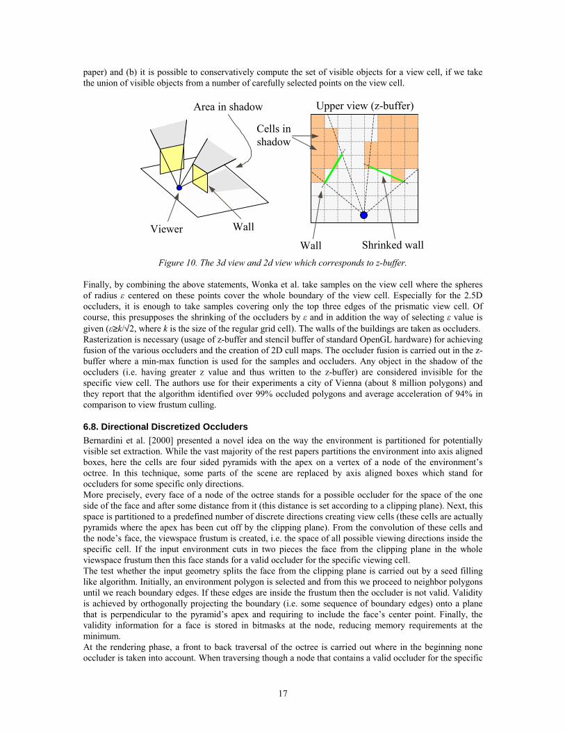
17

paper) and (b) it is possible to conservatively compute the set of visible objects for a view cell, if we take the union of visible objects from a number of carefully selected points on the view cell.

Wall Viewer

Area in shadow

Cells in shadow

Wall Shrinked wall

Upper view (z-buffer)

Figure 10. The 3d view and 2d view which corresponds to z-buffer.

Finally, by combining the above statements, Wonka et al. take samples on the view cell where the spheres of radius ε centered on these points cover the whole boundary of the view cell. Especially for the 2.5D occluders, it is enough to take samples covering only the top three edges of the prismatic view cell. Of course, this presupposes the shrinking of the occluders by ε and in addition the way of selecting ε value is given (ε≥k/√2, where k is the size of the regular grid cell). The walls of the buildings are taken as occluders. Rasterization is necessary (usage of z-buffer and stencil buffer of standard OpenGL hardware) for achieving fusion of the various occluders and the creation of 2D cull maps. The occluder fusion is carried out in the z-buffer where a min-max function is used for the samples and occluders. Any object in the shadow of the occluders (i.e. having greater z value and thus written to the z-buffer) are considered invisible for the specific view cell. The authors use for their experiments a city of Vienna (about 8 million polygons) and they report that the algorithm identified over 99% occluded polygons and average acceleration of 94% in comparison to view frustum culling.

6.8. Directional Discretized Occluders Bernardini et al. [2000] presented a novel idea on the way the environment is partitioned for potentially visible set extraction. While the vast majority of the rest papers partitions the environment into axis aligned boxes, here the cells are four sided pyramids with the apex on a vertex of a node of the environment’s octree. In this technique, some parts of the scene are replaced by axis aligned boxes which stand for occluders for some specific only directions. More precisely, every face of a node of the octree stands for a possible occluder for the space of the one side of the face and after some distance from it (this distance is set according to a clipping plane). Next, this space is partitioned to a predefined number of discrete directions creating view cells (these cells are actually pyramids where the apex has been cut off by the clipping plane). From the convolution of these cells and the node’s face, the viewspace frustum is created, i.e. the space of all possible viewing directions inside the specific cell. If the input environment cuts in two pieces the face from the clipping plane in the whole viewspace frustum then this face stands for a valid occluder for the specific viewing cell. The test whether the input geometry splits the face from the clipping plane is carried out by a seed filling like algorithm. Initially, an environment polygon is selected and from this we proceed to neighbor polygons until we reach boundary edges. If these edges are inside the frustum then the occluder is not valid. Validity is achieved by orthogonally projecting the boundary (i.e. some sequence of boundary edges) onto a plane that is perpendicular to the pyramid’s apex and requiring to include the face’s center point. Finally, the validity information for a face is stored in bitmasks at the node, reducing memory requirements at the minimum. At the rendering phase, a front to back traversal of the octree is carried out where in the beginning none occluder is taken into account. When traversing though a node that contains a valid occluder for the specific

18

viewing direction, then the corresponding face is used for avoiding the rendering of occluded nodes. The test whether another node is occluded from the current list of valid occluders is done on the image plane by keeping occlusion maps. The requirement here is to have the bounding rectangle of the node’s projection to be inside the union of all axis aligned occluder projections. The authors report results over a car model (~162,000 polygons) with an average rendering acceleration of 40%. In some viewer positions though, there is even a decrease of frame rate below the one achieved without culling, something that is explained by the position being too close to the model (a position between the clipping plane and the face acting as an occluder).

6.9. Visibility Octree Saona-Vazquez et al. [1999] presented the idea of shadow frusta to construct the potentially visible sets for the nodes of an octree. Here, the main idea is based on the following theorem: Theorem 1. If A⊆ Rn is a convex set and there exists a plane that separates A from a closed and bounded polyhedron C⊆ Rn with n vertices pi, then:

hn

ii ApSACS

1),(),(

==

Thus, the visibility from a node of the tree (an axis aligned box in the actual implementation) is found from the intersection of the objects visible from each of its vertices. In order to do this, in a preprocessing step all possible occluders are identified (occluders have to be convex and they are selected according to their size) while a bounding volume hierarchy is created. The volumes here are axis aligned boxes bounding the environment objects. It is interesting how the octree, used later in the navigation phase, is constructed. First of all, the visible object lists are found for each node vertex taking into account occluders that are close enough (inside a parallelepiped of side R centered at the vertex). Then, the environment is searched for a polygon separating it from the specific octree node and the visibility is computed (visible bounding volumes for the environment objects) for the two parts by keeping common objects from the lists of the corresponding vertices. Depending on the size of the potentially visible sets of the two parts, the recursive tree construction may end at this level (relatively few visible objects) or may go on by splitting the node (if this successfully leads to reducing the linked visible objects). After the end of preprocessing, the octree (where each node stores the clipping plane and the list of visible objects) is saved along with the bounding volume hierarchy. Simulations were carried out by the authors on a ship model with approximately 110,000 polygons. In the worst case, 40% of the environment was culled while rendering acceleration of more than 300% in comparison to view frustum culling is achieved.

6.10. Selective Refinement Law et al. [1999] describe an occlusion culling technique with simultaneous selection of the detail level of the environment objects. The environment is partitioned into cells (preferring an octree structure) and non visible objects are found for each of them (not only for the leaves but for all hierarchy nodes). This process is done in a preprocessing phase where the selection of the occluders is interesting. Thus, environment polygons are not the only occluders considered but also others that are extracted from a simplification of the scene (virtual occluders). In order for the extracted polygons to be valid, i.e. not occluding objects that are actually visible, after the object simplification a correction process is carried out to bring edges inside the prototype object (edge error correction). Using these extracted polygons, the test for occluded objects is done via their corresponding bounding volume with the technique of supporting planes [Coorg et al. 1997]. Even more, this test is extended for non convex occluders and for more than one occluders sharing a common edge. In the navigation phase, the viewer’s position is followed in the octree in every frame, collecting also the non visible objects or/and non visible parts of multi resolution objects. The visible parts of an object can be smoothed (continuous LOD - selective refinement) starting from the lowest one and increasing resolution and thus avoiding the discontinuities of discrete levels of detail. The authors experiment with various environments, relatively small in size (the biggest one has approximately 45,000 polygons) having large time consuming preprocessing, something that obviously comes from the large number of occluders used. The rendering acceleration varies between 15% and 35%.

19

6.11. Hoops Recently, Brunet et al. [2001] have presented a novel idea of creating special polygonal lines (hoops) that are viewed as convex from specific view cells of the scene. What is interesting about these lines is that they are defined in 3D space and thus their view greatly changes from point to point. From some points they may have the view of self-intersected while from others, they may define the closed boundary of a convex polygon. More specifically, after the creation of a maximal division octree of the environment, for every view cell some seed polygonal lines are created (starting from the biggest black nodes) and evolve taking into account neighbor cells. This extension is done so as the polygonal line projected onto specific planes (planes that are defined for each vertex of the cell as center of projection) represents a simple convex polygon. The usage of these polygonal lines is justified by a basic theorem that states the following: the tests whether the polygonal line is simple for every point in the cell and the same cell is inside a specific area defined by this line (convex appearance polytope) are replaced by corresponding and much simpler tests on the vertices of the cell. The occlusion test is then carried out by checking whether an object is in the shadow of a hoop with respect to a specific cell (this shadow is defined by the supporting planes between the cell and the edges of the hoop). Even more, occluder fusion is supported after finding lines that are partly inside the shadow of another line and then extension of that line to the octree nodes being in its shadow. The authors did experiments with a cathedral model and a folding screen object, where the power of hoops is revealed with the replacement of difficult-to-handle non convex occluders. The technique is characterized as add on to other occlusion culling techniques and thus no comparative results are given.

6.12. Visibility In Terrain The case of terrains is quite different because the environment is not full 3D but represented by functions of the form z=f(x,y) (and many times called “height field”). Stewart [1997] describes a terrain rendering algorithm with simultaneous finding of occluded quadrilaterals and level of detail selection. In the preprocessing phase, for every point of the terrain all the regions that do not “see” it are found. This is carried out with a discretisation of the set of directions into sectors and later finding of the minimum elevation horizon for each point. This is the most critical and time consuming point of the technique (for a terrain of n points, a simple min-max search will result in O(n2) algorithm) and thus an optimized algorithm O(nlog2n) for this task is proposed. The visibility solution for a quadrilateral of the highest resolution is defined by the combination of the visibility results for its vertices. The view point must be inside the intersection of the four occlusion regions for the sectors that are defined by the vertices of the quadrilateral towards the view point (the sectors are found implicitly by finding the minimum and maximum sector between the vertices and the view point). Afterwards, for the quadrilaterals of lower resolution, the occlusion regions are defined by the intersection of the corresponding regions of their child quadrilaterals (quadrilaterals of immediate higher resolution) thus, solving conservatively the visibility problem for all resolutions. In the online process, the first step of the technique is to select the appropriate (lowest) resolution for all points of the terrain, according to the logarithm of the distance from the view point. Then, the hierarchical rendering of the terrain starts from the lowest resolution. If the view point is in the occluded regions of a quadrilateral for all linked sectors, then the quadrilateral is considered occluded, otherwise either the process is repeated for the quadrilateral’s children (with increased resolution) or the quadrilateral is rendered. The latter is carried out if the resolution level of the quadrilateral is higher from all resolutions pre-computed for each of its vertices. The main disadvantage of the technique, besides its large preprocessing time, is the large memory required for storing the occlusion regions of the quadrilaterals. The author chooses not to use (and thus saving memory) the occluded regions linked with the quadrilaterals of the higher resolutions. The speed up for terrains of ~100,000 and ~472,000 points varies from 1 to 2, depending heavily on the view point, while there are view points (in the hardware rendering) where the frame rate decreases.

7. Perspectives The occlusion culling techniques are an active research area for about ten years. Already, complete solutions have been reported [Aliaga et al. 1998, Aliaga et al. 1999] navigating in virtual environments and

20

displaying millions of polygons in real time. It is clear that “mixing” other techniques with occlusion culling, like level of detail adjustment, image based rendering etc. is necessary for fast rendering of realistically complex environments. Of course, specialized hardware, supporting complex occlusion queries (HP graphics hardware already supports basic occlusion queries), needs to be developed towards this direction, so as slow software implementations can be moved away from the cpu. The following table depicts the techniques reviewed in this paper showing their main characteristics and requirements.

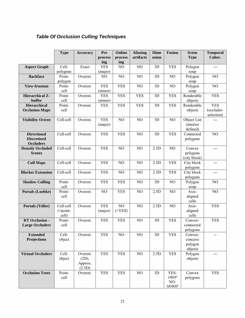
21

Table Of Occlusion Culling Techniques

Type Accuracy Pre process

ing

Online process

ing

Aliasing artifacts

Dimension

Fusion Scene Type

Temporal Coher.

Aspect Graph Cell-polygons

Exact YES (major)

NO NO 3D YES Polygon soup

---

Backface Point-polygon

Overest. NO NO NO 3D NO Polygon soup

NO

View-frustum Point-cell

Overest. YES (minor)

YES NO 3D NO Polygon soup

NO

Hierarchical Z-buffer

Point-cell

Overest. YES (minor)

YES YES 3D YES Renderable objects

YES

Hierarchical Occlusion Maps

Point-cell

Overest. YES YES YES 3D YES Renderable objects

YES (occluder- selection)

Visibility Octree Cell-cell Overest. YES (major)

NO NO 3D NO Object List(interior defined)

---

Directional Discretized Occluders

Cell-cell Overest. YES YES NO 3D YES Connected polygons

NO

Densely Occluded Scenes

Cell-cell Overest. YES NO NO 2.5D NO Convex polygons

(city block)

---

Cull Maps Cell-cell Overest. YES NO NO 2.5D YES City block polygons

---

Blocker Extension Cell-cell Overest. YES NO NO 2.5D YES City block polygons

---

Shadow Culling Point-cell

Overest. YES YES NO 3D NO Polygon soup

NO

Portals (Luebke) Point-cell

Overest. NO YES NO 2.5D NO Axis-aligned

cells

NO

Portals (Teller) Cell-cell (+point-

cell)

Overest. YES (major)

NO (+YES)

NO 2.5D NO Axis-aligned

cells

YES

RT Occlusion - Large Occluders

Point-cell

Overest. YES YES NO 3D YES Convex-connected polygons

YES

Extended Projections

Cell-object

Overest. YES NO NO 3D YES Convex-concave polygon objects

--

Virtual Occluders Cell-object

Overest. (2D),

Approx. (2.5D)

YES YES NO 2.5D YES Polygon objects

---

Occlusion Trees Point-cell

Overest. YES YES NO 3D YES-OBSP NO-

MOBSP

Convex polygons

YES

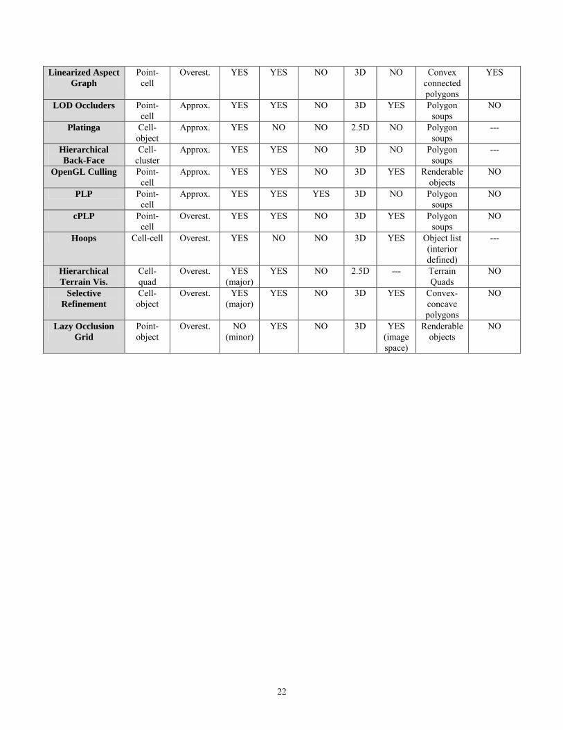
22

Linearized Aspect Graph

Point-cell

Overest. YES YES NO 3D NO Convex connected polygons

YES

LOD Occluders Point-cell

Approx. YES YES NO 3D YES Polygon soups

NO

Platinga Cell-object

Approx. YES NO NO 2.5D NO Polygon soups

---

Hierarchical Back-Face

Cell-cluster

Approx. YES YES NO 3D NO Polygon soups

---

OpenGL Culling Point-cell

Approx. YES YES NO 3D YES Renderable objects

NO

PLP Point-cell

Approx. YES YES YES 3D NO Polygon soups

NO

cPLP Point-cell

Overest. YES YES NO 3D YES Polygon soups

NO

Hoops Cell-cell Overest. YES NO NO 3D YES Object list(interior defined)

---

Hierarchical Terrain Vis.

Cell-quad

Overest. YES (major)

YES NO 2.5D --- Terrain Quads

NO

Selective Refinement

Cell-object

Overest. YES (major)

YES NO 3D YES Convex-concave polygons

NO

Lazy Occlusion Grid

Point-object

Overest. NO (minor)

YES NO 3D YES (image space)

Renderable objects

NO

23

References Airey J., “Increasing Update Rates in the Building Walkthrough System with Automatic Model-Space Subdivision and Potentially Visible Set Calculations”, PhD Thesis, UNC Chapel Hill, 1990.

Aliaga D., Cohen J., Wilson A., Zhang H., Erikson C., Hoff K., Hudson T., Stuerzlinger W., Baker E., Bastos R., Whitton M., Brooks F. and Manocha D., “A Framework for the Real-Time Walkthrough of Massive Models”, UNC Technical Report #98-013, March, 1998.

Aliaga D., Cohen J., Wilson A., Baker E., Zhang H., Erikson C., Hoff K., Hudson T., Stuerzlinger W., Bastos R., Whitton M., Brooks F. and Manocha D., “MMR: An Interactive Massive Model Rendering System using Geometric and Image-Based Acceleration”, Proc. Symposium on Interactive 3D Graphics (I3D), ACM Press, New York, pp. 199-206, April, 1999.

Andujar C., Saona-Vazquez C. and Navazo I., “LOD Visibility Culling and Occluder Synthesis”, Computer Aided Design, Vol. 32, No. 13, pp. 773-783, 1999.

Andujar C., Saona-Vazquez C., Navazo I. and Brunet P., “Integrating Occlusion Culling and Levels of Detail through Hardly-Visible Sets”, Proc. Eurographics 2000, Gross M. and Hopgood F. R. A. (editors), Vol. 19, No. 3, 2000.

Assarsson U. and Moller T., “Optimized View Frustum Culling for Bounding Boxes”, Journal of Graphics Tools, Vol. 5, No. 1, pp. 9-22, 2000.

Bartz D., Meisner M. and Huttner T., “OpenGL-assisted Occlusion Culling for Large Polygonal Models”, Computer and Graphics, Vol. 23, No. 5, 1999.

Bentley J. L., “Multidimensional Binary Search Trees used for Associative Searching”, Communications of ACM, Vol. 18, pp. 509-517, 1975.

Bernardini F., El-Sana J. and Klosowski J. T., “Directional Discretized Occluders for Accelerated Occlusion Culling”, Proc. Eurographics ‘2000, Gross M. and Hopgood F. R. A. (editors), Vol. 19, No. 3, 2000.

Bittner J., Havran V. and Slavic P., “Hierarchical Visibility Culling with Occlusion Trees”, Proc. of CGI '98, IEEE, New York, pp. 207-219, 1998.

Brunet P., Navazo I., Rossignac J. and Saona-Vazquez C., “Hoops: 3D Curves as Conservative Occluders for Cell-Visibility”, Eurographics 2001, Chalmers A. and Rhyne T.-M. (editors), Vol. 20, No. 3, 2001.

Chakravarty I. and Freeman H., “Charasteristic views as a basis for three-dimensional object recognition”, Proc. SPIE, Vol. 336 (Robot Vision), pp. 37-45, 1982.

Chin N. and Feiner S., “Near real-time shadow generation using BSP trees”, Proc. of SIGGRAPH ’90, pp. 99-106, August 1990.

Cohen-Or D., Fibich G., Halperin D. and Zadicario E., “Conservative Visibility and Strong Occlusion for Viewspace Partitioning of Densely Occluded Scenes”, Proc. Eurographics ’98, Vol. 17, No. 3, 1998.

Cohen-Or D., Chrysanthou Y. and Silva C. T., “A Survey of Visibility for Walkthrough Applications”, Proc. of Eurographics '2000, course notes, 2000.

Coorg S. and Teller S., “Temporally Coherent Conservative Visibility”, Symp. on Computational Geometry, pp. 78-87, 1996.

Coorg S. and Teller S., “Real-Time Occlusion Culling for Models with Large Occluders”, Proc. ACM Symp. on Interactive 3D Graphics, pp. 83-90, 1997.

Dorward S. E., “A Survay of Object-Space Hidden Surface Removal”, Intern. J. Comput. Geom. Appl., Vol. 4, pp. 325-362, 1994.

24

Durand F., Drettakis G. and Puech C., “The 3d visibility complex, a new approach to the problems of accurate visibility”, Proc. 7th Eurographics Workshop on Rendering, Pueyo X. and Shroder P. editors, Springer-Verlag, pp. 245-257, Porto, Portugal, June 1996.

Durand F., Drettakis G. and Puech C., “The visibility skeleton: A powerful and efficient multi-purpose global visibility tool”, Computer Graphics (Siggraph ’97 Proceedings), pp. 89-100, 1997.

Durand F., Drettakis G., Thollot J. and Puech C., “Conservative Visibility Preprocessing using Extended Projections”, SIGGRAPH 2000, ACM Press, Addison-Wesley, New York, pp. 239-248, 2000.

Fujimoto A., Tanaka T. and Iwata K., “Arts: Accelerated ray-tracing system”, IEEE Computer Graphics and Applications, Vol. 6, No. 4, pp. 16--26, April 1986.

Gigus Z., Canny J. and Seidel R., “Efficiently computing and representing aspect graphs of polyhedral objects”, Proc. 2nd Int. Conf. and Computer Vision, pp. 20-29, 1988.

Goldsmith J. and Salmon J., “Automatic Creation of Object Hierarchies for Ray Tracing”, IEEE Computer Graphics and Applications, Vol. 7, No. 5, pp. 14-20, May 1987.

Green N., Kass M. and Miller G., “Hierarchical Z-Buffer Visibility”, Proc. of ACM Siggraph, pp. 231-238, 1993.

Green N. and Kass M., “Error Bounded Antialiased Rendering in Complex Environments”, SIGGRAPH ’94 Conference Proceedings, pp. 59-66, 1994.

Haines A. E. and Wallace J. R., “Shaft Culling for Efficient Ray Cast Radiosity”, Proc. of the 2nd Eurographics Workshop on Rendering, P. Brunet and F. W. Jansen editors, Springer-Verlag, New York, 1994.

Hey H., Tobler R. F. and Purgathofer W., “Real-Time Occlusion Culling with a Lazy Occlusion Grid”, Technical Report TR-186-2-01-02, Institute of Computer Graphics and Algorithms, Vienna University of Technology, Jan. 2001.

Hudson T., Manocha D., Cohen J., Lin M., Hoff K. and Zhang H., “Accelerated Occlusion Culling using Shadow Frusta”, Proc. 13th Symp. Computational Geometry, ACM Press, pp. 1-9, June 1997.

Klosowski J. T. and Silva C. T., “Rendering on a Budget: A Framework for Time-Critical Rendering”, IEEE Transactions on Visualization and Computer Graphics, Vol. 6, No. 2, pp. 108-123, 2000.

Klosowski J. T. and Silva C. T., “Efficient Conservative Visibility Culling Using The Prioritized-Layered Projection Algorithm”, IEEE Transactions on Visualization and Computer Graphics, 2001 (to appear).

Koenderink J. J. and van Doorn A. J., “The Internal Representation of solid shape with respect to vision”, Biol. Cybernet., Vol. 32, pp. 211-216, 1979.

Koltun V., Chrysanthou Y. and Cohen-Or D., “Virtual Occluders: An Efficient Intermediate PVS representation”, Proc. 11th Eurographics Workshop on Rendering, 2000.

Kumar S., Manocha D., Garrett B. and Lin M., “Hierarchical Back-Face Computation”, Proc. of Eurographics Workshop on Rendering, pp. 231-240, June 1996 (Computers & Graphics, Vol. 23, No. 5, pp. 681-692, October 1999).

Law F.-A. and Tan T.-S., “Preprocessing Occlusion for Real-Time Selective Refinement”, Symp. on Interactive 3D Graphics, Atlanta GAUSA, ACM Press, pp. 47-53, 1999.

Luebke D. P. and Georges C., “Portals and Mirrors: Simple, Fast Evaluation of Potentially Visible Sets”, Proc. of the 1995 Symposium on Interactive 3-D Graphics, ACM Press, pp. 105-ff., April 1995.

Meagher D., “Geometric Modeling using Octree Encoding”, Computer Graphics and Image Processing, Vol. 19, pp. 129-147, 1982.

Platinga H. and Dyer C. R., “An algorithm for constructing the aspect graph”, Proc. 27th Ann. Symp. on Foundations of Computer Sci., pp. 123-131, 1986.

25

Platinga H. and Dyer C. R., “Visibility, occlusion, and the aspect graph”, Technical Report 736, University of Wisconsin - Madison, December 1987.

Platinga H., “Conservative Visibility Preprocessing for Efficient Walkthroughs of 3D Scenes”, Proc. Graphics Interface ’93, pp. 166-173, 1993.

Pocchiola M. and Vegter G., “The visibility complex”, Int. J. Comput. Geom. Appl., special issue devoted to ACM-SoCG ’93, 1993.

Saona-Vazquez C., Navazo I. And Brunet P., “The Visibility Octree. A Data Structure for 3D Navigation”, Computers & Graphics, Vol. 23, No. 5, pp. 635-643, 1999.

Schaufler G., Dorsey J., Decoret X. and Sillion F. X., “Conservative Volumetric Visibility with Occluder Fusion”, Proc. SIGGRAPH 2000, pp. 229-238, 2000.

Scott N., Olsen D. and Gannett E., “An Overview of the VISUALIZE fx Graphics Accelerator Hardware”, The Hewlett-Packard Journal, pp. 28-34, May 1998.

Stewart J. A., “Hierarchical Visibility in Terrains”, Proc. Eurographics RenderingWorkshop, pp. 217-228, June 1997.

Stewman J. and Bowyer K., “Creating the perspective projection aspect graph of polyhedral objects”, Proc. Second Int. Conf. on Computer Vision, pp. 494-500, 1988.

Teller S. and Sequin C., “Visibility Preprocessing for Interactive Walkthroughs”, Computer Graphics, Vol. 25, No. 4, pp. 61-68, 1991.

Wonka P., Wimmer M. and Schmalstieg D., “Visibility Preprocessing with Occluder Fusion for Urban Walkthroughs”, Technical Report TR-186-2-00-06, March 2000.

Xie F. and Shantz M., “Adaptive Hierarchical Visibility in a Tiled Architecture”, ACM Press, New York, pp. 75-84, 1999.

Yamaguchi K., Kunii T. L., Fujimura K. and Toriya H., “Octree Related Data Structures and Algorithms”, IEEE Computer Graphics and Applications, Vol. 4, No. 1, pp. 53-59, 1984.

Zhang H., Manocha D., Hudson T. and Hoff K., “Visibility Culling Using Hierarchical Occlusion Maps”, Proc. of SIGGRAPH ’97, ACM Press, Addison-Wesley, New York, pp. 77-88, 1997.