Observer based feedforward/feedback control of

electro-pneumatic clutch systems

Ph.D. Thesis

Barna Szimandl

Supervisor: Huba Németh

Kálmán Kandó Doctoral School of Transportation Engineering

Transportation and vehicle engineering sciences

Budapest University of Technology and Economics

Faculty of Transportation Engineering

Department of Automobiles and Vehicle Manufacturing

Budapest, Hungary

2015

Abstract

This dissertation deals the with control of electro-pneumatic clutch systems applied in mediumand heavy duty commercial vehicles. The main goal of the thesis is to build up a dynamic modelof the system, to prepare and apply a model simplification approach, to analyze the dynamicproperties of the simplified models and to develop a clutch controller using the nonlinear modelof the electro-pneumatic clutch.

It is shown that the electro-pneumatic clutch system can be described as a mixed thermody-namic, mechanic and electro-magnetic system and its model can be build and verified by usinga systematic modeling methodology. The developed model structure is valid for clutch systemsapplied with concentric and forked lever type electro-pneumatic clutch actuators as well, onlythe model parameters differ from each other. The model exhibits hybrid, i.e. discrete-continuousbehavior caused by different elements with inherently discrete behavior. The model has beenverified and then validated against laboratory measurements. It has been shown that it is ableto describe the dynamic behavior of the modeled system within the predefined tolerance limit.

A systematic model simplification process has been applied to the detailed model of theelectro-pneumatic clutch. Two simplified models have been constructed: one for fast simulationand an other one for control design purpose. The size of the state vector has been reduced and thestructure of the algebraic equations has been simplified considerably in both cases. The discretecomponents of the models have been eliminated completely in case of the control oriented model.It has been shown that all retained system variable entries of the simplified models preservedtheir physical meaning and the control oriented model can be rewritten into standard input affineform.

When performing model analysis for the control oriented model, it has been proved that thismodel is jointly reachable and detectable, thus it is minimal. The stability analysis has shownthat the global asymptotic stability of the open loop model depends on model parameters. Theasymptotic stability of the zero dynamics has been proved, thus the system is locally asymptot-ically stabilizable and asymptotic output tracking is achievable with appropriate feedback.

Based on the control aims and the input signal constraints an observer basedfeedforward/feedback controller structure has been developed. It includes three blocks in formof a state observer supplying the unmeasurable states, a feedforward controller unit producingthe mass flow rate control and the I/O linearization of the solenoid magnet valves, and a modelbased feedback controller unit provides a piston position control. For the state observer thehigh-gain observer method has been used. For the feedforward and the feedback controllersseveral approaches have been considered, such as the static- and dynamic mass flow rate de-composition approach, the linear quadratic, robust H∞ and sliding mode control approach. Theobtained closed loops are investigated by extensive simulation, bench- and vehicle tests to verifythe properties of the different controls.

ii

Tartalmi kivonat

A disszertáció közepes és nehéz haszongépjárművekben alkalmazott elektro-pneumatikustengelykapcsolók irányításával foglalkozik. A vizsgálat tárgya az elektro-pneumatikustengelykapcsolók dinamikus modellezése, a modell meghatározott célra való egyszerűsítése, amodell dinamikus analízise valamint egy modell alapú tengelykapcsoló szabályozó tervezése és atervezett szabályozó tulajdonságainak ellenőrzése.

A vizsgálat megmutatta, hogy az elektro-pneumatikus tengelykapcsoló működtető egy vegyestermodinamikai, mechanikai és elektro-dinamikai rendszer, amelynek modellje szisztematikusmodellezési eljárással felépíthető és verifikálható. A különböző elektro-pneumatikustengelykapcsoló kialakítások modellstruktúrája azonos, csak a modell paraméterekbenkülönböznek egymástól. Az így felépített nemlineáris dinamikus hibrid modell speciálisstruktúrájú, diszkrét és folytonos elemeket is tartalmaz. A modell érvényességének ellenőrzéselaboratóriumi mérések segítségével történt. A vizsgálat bebizonyította, hogy a modell alkalmasa valós rendszer dinamikus viselkedésének megadott tolerancia szinten belüli leírására.

A fizikai törvényszerűségek felhasználásával megalkotott modellt a szerző továbbegyszerűsítette. E célból egy szisztematikus modellegyszerűsítési eljárást alkalmazott éskét egyszerűsített modellt alkotott meg: egyet gyors szimulációs célokra és egy másikatszabályozó-tervezés céljára. A modell egyszerűsítése révén csökkent az állapot vektor dimenziójaés jelentősen egyszerűsödött az egyenletek algebrai alakja mind a két esetben. A vizsgálatkimutatta, hogy a rendszer változói megtartják fizikai jelentésüket. A diszkrét-folytonos elemeketa szabályozó-tervezés céljára egyszerűsített modell esetén a szerző teljesen kiküszöbölte, valaminta modellt standard input affin alakra hozta.

A modell analízise során a szerző kimutatta, hogy a szabályozó-tervezés céljára egyszerűsítettmodell együttesen elérhető és detektálható, azaz a modell minimális reprezentációjú. A nyitottrendszer stabilitási vizsgálata megmutatta, hogy a modell globális asszimptotikus stabilitásafügg a modell paramétereitől. Ezenkívül a szerző azt is igazolta, hogy az egyszerűsített modellmaximális relatív fokszámmal rendelkezik, így a zérus dinamika aszimptotikusan stabil. Ezzela rendszer lokálisan aszimptotikusan stabilizálható és aszimptotikus jelkövetés valósítható megegy megfelelő visszacsatolással.

A szabályozási célok és a bemeneti jelre előírt korlátozás alapján egy megfigyelő alapúelőrecsatolt/visszacsatolt szabályozó struktúra került kifejlesztésre. A szabályozási struktúrahárom blokkot tartalmaz: egy állapot megfigyelőt mely a nem mérhető állapotot állítja elő, egyelőrecsatoló egységet mely az elektro-pneumatikus tengelykapcsoló mőködtetőben alkalmazottszelepek légtömegáram vezérlését és I/O linearizálását valósítja meg és egy visszacsatoló egységetmely a mőködtető dugattyú pozíciójának szabályozását biztosítja. Az állapot megfigyelőesetén egy nagy-erősítésű megfigyelő került kidolgozásra. Az előrecsatolt és visszacsatoltirányítások esetén különböző megoldásokat vizsgált meg a szerző, úgymint statikus és dinamikuslégtömegáram felbontás, lineáris kvadratikus, robusztus H∞ és csúszó mód irányítás. Akidolgozott szabályozási rendszereket kiterjedt szimulációs-, tesztpadi és járműves tesztekkelellenőrizte a szerző.

iii

Foreword

This thesis summarizes the contributions of my research work for obtaining Ph.D. degree inKálmán Kandó Doctoral School of Transportation Engineering at the Faculty of TransportationEngineering of the Budapest University of Technology and Economics. The scientific part of thestudies has been undertaken at the Knorr-Bremse Research and Development Centre Budapest.

This work would have never been written without the help, continuous support and encour-agement of several people. First of all, I want to express my sincere gratitude to my supervisor,head of the Advanced Engineering Group at Knorr-Bremse R&D Center Budapest and asso-ciate professor of Budapest University of Technology and Economics Faculty of TransportationEngineering Department of Automobiles and Vehicle Manufacturing, Dr. Huba Németh, forhis patient guidance throughout my studies and support for realizing the opportunities for theexperiments.

I would like to express my gratitude to Professor József Bokor, the head of Systems andControl Laboratory and his colleagues for providing me with the essential ideas and literatureon dynamic systems and control. I am also grateful to my colleagues, Zoltán Geiszt and BalázsTrencséni for the joint work.

Finally, I am grateful to my wife Ági, my parents and my friends for supporting my studiesin many ways for such a long time.

The undersigned, Barna Szimandl declares that this Ph.D. thesis has been prepared by himselfas well as that the indicated sources have been used only. All parts that have been taken overliterally or by content are cited unambiguously.

Alulírott Szimandl Barna kijelentem, hogy ezt a doktori értekezést magam készítettem ésabban csak a megadott forrásokat használtam fel. Minden olyan részt, amelyet szó szerint, vagyazonos tartalomban, de átfogalmazva más forrásból átvettem, egyértelműen, a forrás megadásávalmegjelöltem.

Budapest, 2015.06.30. . . . . . . . . . . . . . . . . . . . . . . . . . . . . . .Szimandl Barna

iv

Contents

Abstract ii

Tartalmi kivonat iii

Foreword iv

Contents vii

List of Figures viii

List of Tables 1

1 Introduction 11.1 Problem statement and motivation . . . . . . . . . . . . . . . . . . . . . . . . . . 11.2 Electro-pneumatic clutch systems and their control . . . . . . . . . . . . . . . . . 21.3 The aim of the work . . . . . . . . . . . . . . . . . . . . . . . . . . . . . . . . . . 31.4 Layout of the thesis . . . . . . . . . . . . . . . . . . . . . . . . . . . . . . . . . . 31.5 Nomenclature . . . . . . . . . . . . . . . . . . . . . . . . . . . . . . . . . . . . . . 4

2 Nonlinear dynamic hybrid model 72.1 System definition . . . . . . . . . . . . . . . . . . . . . . . . . . . . . . . . . . . . 72.2 Modeling: goals and approaches . . . . . . . . . . . . . . . . . . . . . . . . . . . . 92.3 Simplifying assumptions and input constraints . . . . . . . . . . . . . . . . . . . . 102.4 Conservation equations . . . . . . . . . . . . . . . . . . . . . . . . . . . . . . . . . 12

2.4.1 Conservation of gas mass in the clutch actuator chamber V1 . . . . . . . . 122.4.2 Conservation of gas energy in the clutch actuator chamber V1 . . . . . . . 132.4.3 Conservation of clutch actuator piston momentum V2 . . . . . . . . . . . 132.4.4 Conservation of SMV armature momentum V3−6 . . . . . . . . . . . . . . 142.4.5 Conservation of magnetic linkage in the SMVs V9−10 . . . . . . . . . . . . 15

2.5 Constitutive equations . . . . . . . . . . . . . . . . . . . . . . . . . . . . . . . . . 162.5.1 Chamber and gas properties . . . . . . . . . . . . . . . . . . . . . . . . . . 162.5.2 SMV airflow properties . . . . . . . . . . . . . . . . . . . . . . . . . . . . . 172.5.3 Forces acting on the piston . . . . . . . . . . . . . . . . . . . . . . . . . . 172.5.4 Forces acting on the SMV armature . . . . . . . . . . . . . . . . . . . . . 182.5.5 Electro-magnetic relations . . . . . . . . . . . . . . . . . . . . . . . . . . . 202.5.6 Power stage relations . . . . . . . . . . . . . . . . . . . . . . . . . . . . . . 20

2.6 Hybrid items . . . . . . . . . . . . . . . . . . . . . . . . . . . . . . . . . . . . . . 212.6.1 Power stage voltage drop . . . . . . . . . . . . . . . . . . . . . . . . . . . 212.6.2 SMV airflow term . . . . . . . . . . . . . . . . . . . . . . . . . . . . . . . 21

v

2.6.3 Armature stroke dependent terms of the valves . . . . . . . . . . . . . . . 212.6.4 Piston stroke limiting forces . . . . . . . . . . . . . . . . . . . . . . . . . . 222.6.5 Piston friction force . . . . . . . . . . . . . . . . . . . . . . . . . . . . . . 22

2.7 Model equations in state space form . . . . . . . . . . . . . . . . . . . . . . . . . 232.7.1 State equations . . . . . . . . . . . . . . . . . . . . . . . . . . . . . . . . . 232.7.2 Output equations . . . . . . . . . . . . . . . . . . . . . . . . . . . . . . . . 25

2.8 Model verification and validation . . . . . . . . . . . . . . . . . . . . . . . . . . . 262.8.1 Disengagement process verification . . . . . . . . . . . . . . . . . . . . . . 262.8.2 Engagement process verification . . . . . . . . . . . . . . . . . . . . . . . . 282.8.3 Validation . . . . . . . . . . . . . . . . . . . . . . . . . . . . . . . . . . . . 29

2.9 Summary . . . . . . . . . . . . . . . . . . . . . . . . . . . . . . . . . . . . . . . . 34

3 Model simplification 363.1 Structure of the dynamic hybrid model . . . . . . . . . . . . . . . . . . . . . . . . 363.2 Model simplification procedure . . . . . . . . . . . . . . . . . . . . . . . . . . . . 393.3 Simplification results . . . . . . . . . . . . . . . . . . . . . . . . . . . . . . . . . . 40

3.3.1 Simplified nonlinear dynamic hybrid model for simulation purposes (M1) 403.3.2 Simplified nonlinear dynamic model for control design purposes (M2) . . 45

3.4 Summary . . . . . . . . . . . . . . . . . . . . . . . . . . . . . . . . . . . . . . . . 47

4 Model analysis 494.1 Controllability . . . . . . . . . . . . . . . . . . . . . . . . . . . . . . . . . . . . . 504.2 Observability . . . . . . . . . . . . . . . . . . . . . . . . . . . . . . . . . . . . . . 514.3 Stability . . . . . . . . . . . . . . . . . . . . . . . . . . . . . . . . . . . . . . . . . 51

4.3.1 Stability analysis applying Lyapunov’s indirect method . . . . . . . . . . . 554.3.2 Stability analysis applying Lyapunov’s direct method . . . . . . . . . . . . 56

4.4 Zero dynamics . . . . . . . . . . . . . . . . . . . . . . . . . . . . . . . . . . . . . 584.5 Sensitivity . . . . . . . . . . . . . . . . . . . . . . . . . . . . . . . . . . . . . . . . 584.6 Summary . . . . . . . . . . . . . . . . . . . . . . . . . . . . . . . . . . . . . . . . 59

5 Control design 615.1 Requirements on the clutch control . . . . . . . . . . . . . . . . . . . . . . . . . . 615.2 Controller structure . . . . . . . . . . . . . . . . . . . . . . . . . . . . . . . . . . 625.3 Piston position control . . . . . . . . . . . . . . . . . . . . . . . . . . . . . . . . . 63

5.3.1 Linear quadratic approach . . . . . . . . . . . . . . . . . . . . . . . . . . . 635.3.2 H∞ approach with exact linearization . . . . . . . . . . . . . . . . . . . . 655.3.3 Sliding mode control approach . . . . . . . . . . . . . . . . . . . . . . . . 68

5.4 Mass flow rate control . . . . . . . . . . . . . . . . . . . . . . . . . . . . . . . . . 705.4.1 Static mass flow rate decomposition approach . . . . . . . . . . . . . . . . 705.4.2 Dynamic mass flow rate decomposition approach . . . . . . . . . . . . . . 71

5.5 State observer . . . . . . . . . . . . . . . . . . . . . . . . . . . . . . . . . . . . . . 745.6 Experimental results . . . . . . . . . . . . . . . . . . . . . . . . . . . . . . . . . . 76

5.6.1 Simulation test . . . . . . . . . . . . . . . . . . . . . . . . . . . . . . . . . 785.6.2 Clutch bench test . . . . . . . . . . . . . . . . . . . . . . . . . . . . . . . . 825.6.3 Vehicle test . . . . . . . . . . . . . . . . . . . . . . . . . . . . . . . . . . . 84

5.7 Summary . . . . . . . . . . . . . . . . . . . . . . . . . . . . . . . . . . . . . . . . 87

vi

6 Conclusions 886.1 Theses . . . . . . . . . . . . . . . . . . . . . . . . . . . . . . . . . . . . . . . . . . 886.2 Publications . . . . . . . . . . . . . . . . . . . . . . . . . . . . . . . . . . . . . . . 90

6.2.1 Publications directly related to the thesis . . . . . . . . . . . . . . . . . . 906.2.2 Submitted patents . . . . . . . . . . . . . . . . . . . . . . . . . . . . . . . 916.2.3 Other publications . . . . . . . . . . . . . . . . . . . . . . . . . . . . . . . 91

6.3 Directions for future research . . . . . . . . . . . . . . . . . . . . . . . . . . . . . 91

Bibliography 93

Appendix A Figures and Tables 100

Appendix B Model transformations 103B.1 Linearization around a steady state point x∗ . . . . . . . . . . . . . . . . . . . . . 103B.2 Coordinate transformation . . . . . . . . . . . . . . . . . . . . . . . . . . . . . . . 104B.3 Exact linearization via state feedback . . . . . . . . . . . . . . . . . . . . . . . . . 106

List of Figures

2.1 The layout of the electro-pneumatic clutch (EPC) system . . . . . . . . . . . . . 82.2 Free body diagram of the piston . . . . . . . . . . . . . . . . . . . . . . . . . . . . 142.3 Free body diagram of the solenoid magnet valve (SMV) armature . . . . . . . . . 152.4 Magnetic linkage in the solenoid . . . . . . . . . . . . . . . . . . . . . . . . . . . . 152.5 Two way two port on/off SMV layout . . . . . . . . . . . . . . . . . . . . . . . . . 172.6 Characteristic of the clutch mechanism Fl (xpst) . . . . . . . . . . . . . . . . . . . 192.7 Transient of the valve signals during disengagement . . . . . . . . . . . . . . . . . 272.8 Transient of the chamber/piston states during disengagement . . . . . . . . . . . 282.9 Transient of the valve signals during engagement . . . . . . . . . . . . . . . . . . 292.10 Transient of the chamber/piston states during engagement . . . . . . . . . . . . . 302.11 Transient of the terminal voltages and currents during disengagement . . . . . . . 312.12 Transient of the terminal voltages and currents during engagement . . . . . . . . 322.13 Transient of the pressure and position during disengagement . . . . . . . . . . . . 322.14 Transient of the pressure and position during engagement . . . . . . . . . . . . . 332.15 Real clutching procedure in case of gear shifting . . . . . . . . . . . . . . . . . . . 34

3.1 Structure graph of the differential variables of the EPC model . . . . . . . . . . . 373.2 Hierarchical structure of the detailed nonlinear dynamic hybrid model . . . . . . 383.3 Model simplification procedure . . . . . . . . . . . . . . . . . . . . . . . . . . . . 393.4 EPC measurement and simulation results in case of model M0, M1 and M2 . . 433.5 Hierarchical structure of the simplified model M1 . . . . . . . . . . . . . . . . . . 443.6 Structure graph of the differential variables of the simplified model M1 . . . . . . 453.7 Model performance and size indices in case of model M0, M1 and M2 . . . . . . 463.8 Hierarchical structure of the simplified model M2 . . . . . . . . . . . . . . . . . . 483.9 Structure graph of the differential variables of the simplified model M2 . . . . . . 48

4.1 Equilibrium points over the pressure-position plane with increasing dead volume 57

vii

4.2 Sensitivity of the states regarding the model parameters . . . . . . . . . . . . . . 60

5.1 Structure of the observer based feedforward/feedback control . . . . . . . . . . . 625.2 LQ servo block structure . . . . . . . . . . . . . . . . . . . . . . . . . . . . . . . . 645.3 Closed loop interconnection structure . . . . . . . . . . . . . . . . . . . . . . . . . 655.4 The ∆-P-K structure . . . . . . . . . . . . . . . . . . . . . . . . . . . . . . . . . . 665.5 Singular values with full order controller regarding RS, NP and RP . . . . . . . . 675.6 Singular values with full and reduced order controllers . . . . . . . . . . . . . . . 675.7 High-gain anti-windup structure . . . . . . . . . . . . . . . . . . . . . . . . . . . . 685.8 Available mass flow rates plotted against different chamber pressure . . . . . . . . 715.9 Mass flow rates of ideal, proportional and real valves . . . . . . . . . . . . . . . . 725.10 Characteristics of small SMVs . . . . . . . . . . . . . . . . . . . . . . . . . . . . . 735.11 Characteristics of big SMVs . . . . . . . . . . . . . . . . . . . . . . . . . . . . . . 745.12 Magnitude and phase of the frequency response from y to x, ˙x and to ¨x . . . . . 775.13 Graphical interpretation of the performance indices . . . . . . . . . . . . . . . . . 785.14 Step responses with 100% stroke in case of simplified model . . . . . . . . . . . . 795.15 Clutch engagement test functions in case of simplified model . . . . . . . . . . . . 795.16 Step responses with 100% stroke in case of detailed model . . . . . . . . . . . . . 815.17 Clutch engagement test functions in case of detailed model . . . . . . . . . . . . . 815.18 Electro-pneumatic clutch system layout . . . . . . . . . . . . . . . . . . . . . . . 825.19 Step responses with 100% stroke in case of test bench . . . . . . . . . . . . . . . 835.20 Clutch engagement test functions in case of test bench . . . . . . . . . . . . . . . 835.21 The sliding surface and the state trajectory in the phase plane . . . . . . . . . . . 845.22 Smooth launch of the vehicle . . . . . . . . . . . . . . . . . . . . . . . . . . . . . 855.23 Dynamic launch and gearshifting . . . . . . . . . . . . . . . . . . . . . . . . . . . 86

A.1 Friction disc, clutch mechanism and concentric clutch actuator from ZF SACHS . 100A.2 Engine, gearbox and clutch system . . . . . . . . . . . . . . . . . . . . . . . . . . 101A.3 Clutch systems applied with forked lever- and concentric type EPC actuators . . 101

B.1 Block diagram of the exact linearization via state feedback . . . . . . . . . . . . . 106

List of Tables

2.1 Balance volumes and conserved quantities . . . . . . . . . . . . . . . . . . . . . . 122.2 Hybrid modes of the power stage voltage drop . . . . . . . . . . . . . . . . . . . . 212.3 Hybrid modes of the air flow . . . . . . . . . . . . . . . . . . . . . . . . . . . . . . 222.4 Hybrid modes of the armature stroke dependent terms . . . . . . . . . . . . . . . 222.5 Hybrid modes of the clutch actuator piston limiting forces . . . . . . . . . . . . . 222.6 Hybrid modes of the Friction forces . . . . . . . . . . . . . . . . . . . . . . . . . . 232.7 Accuracy and range of measured signals . . . . . . . . . . . . . . . . . . . . . . . 302.8 The modeling errors in case of nonlinear dynamic hybrid model . . . . . . . . . . 35

5.1 Performance indices of step response and clutch slipping tests . . . . . . . . . . . 80

A.1 List of parameters . . . . . . . . . . . . . . . . . . . . . . . . . . . . . . . . . . . 102

viii

Chapter 1

Introduction

”The science of today is the technology of tomorrow.”Ede Teller

1.1 Problem statement and motivation

The automotive industry is one of the leading industry branches all around the world. The mainreason of this fact is that this is the primary field of ”civil” application of the newest scientificresults reached in the space, aviation and military research, as well as a good trial opportunityfor the new innovations in other scientific areas. No doubt, the passenger car development,application of new ideas and technology is the leading area compared to the other road vehiclesystems. The explanation for it is obvious: the price of passenger cars, usually bought for pleasurerather than making profit, can incorporate the extra costs of the advanced systems. This isthe ground for the wide application of controlled vehicle systems in passenger cars: anti-lockbraking system, traction control system, electronic engine control, semi-active and/or adaptivesuspension controls are all standard in even medium size passenger cars. The application ofadvanced, electronically controlled systems in commercial vehicles somehow has not been as fastas in the passenger cars in the past. The explanation of this situation shows the constraints forthe development and marketing of these systems:

1. The primary reason why a commercial vehicle is purchased in business like: making profit,which means low price of the vehicle, low maintenance cost, reliability throughout the lifecycle of the vehicle. This fact is contradictory to the application of any advanced system,since normally they make the vehicle more expensive, although their impact on the vehiclesafety and on the costs of operation is obviously advantageous.

2. The commercial vehicle market is more conservative, does not like to accept new systemsunless it is convinced about the definitive advantages. Typical example is the reluctance ofthe market concerning the electro-pneumatic brake systems for heavy commercial vehicles,whereas the advantages are obvious, but people ”would not see” the brake actuation (i.e.there are no pneumatic lines, tubes, valves to control the wheel brake) since it is doneelectronically. This was the reason (besides the legislation) that redundant pneumaticcircuits had to be installed in parallel to the otherwise very safe electronic brake system.

However, with growing number of the vehicles all around the world, the demand of the societyon the traffic safety is also increasing. Since the transportation infrastructure cannot keep upwith rising number of vehicles there is a severe task for the transportation as well as control andmechanical engineers to control the traffic flow in the way of enhancing traffic safety and, at the

1

same time, increasing the efficiency of the transportation, i.e. increasing the traffic density. Asseen, there is an obvious contradiction between the mentioned two facts, since increasing thetraffic density will result in growing probability of traffic accidents. This contradiction cannotbe relieved, but it can be optimized by a certain way, giving intelligence both to the vehicleitself, and also to the infrastructure, making the information flow between the road and the carpossible.

These and similar requirements explain the need of the society for safer, less polluting, lessdangerous and last but not least less expensive heavy vehicles, which have no significantly differ-ent performance as the passenger cars. These fact make the development of commercial vehicleadvanced systems more interesting and more challenging for development engineers and scien-tists, since to fulfill all the technical conditions, at relatively lower price, resulting in a lesscomplex system is not an easy task [1].

An important part of this innovation of commercial vehicles is to improve the control ofelectron-pneumatic clutch systems to achieve high dynamics and accurate signal tracking.

1.2 Electro-pneumatic clutch systems and their control

The requirements of the clutch control function are determined by the controllability of thetorque, transmitted by the clutch. The transmitted torque is a function of the piston positionof the clutch actuator realized by a disc spring, therefore the position control can provide clutchtorque control function.

In the last decade, several papers have been published on the topic of the position control ofelectro-pneumatic clutch actuators. These actuators are driven by proportional- or on/off valves,which yield that the control signals can be continuous and have to be quantized respectively.

One of the proposed control methods are the PID type controls, extended with self-tuningability using parallel feedforward compensator, neural network or fuzzy proportional summationand derivative (PSD) methods [2, 3, 4]. These controls are designed for clutch actuators withproportional valves. Other published methods are the switching controls, in which a controlLyapunov function is defined to achieve exponential stability in the operation domain usingquantized control input, where the quantization came from applying on/off valves instead ofproportional ones [5, 6, 7, 8]. Explicit model predictive control techniques are also used, wherethe minimization of a cost function in a finite horizon is performed off-line [9, 10, 11].

Comparing these methods above, it can say that, nonlinear methods can achieve higherdisturbance rejection performance and wider stability margin versus linear ones. In Lyapunovfunction based switching controls a stabilizing controller is defined first and a switching surfaceis found from this. It is more straightforward to provide a predefined dynamic behavior on aswitching surface, e.g. in case of sliding mode control, to achieve the desired performance of thesystem easily. Model predictive controls may not provide acceptable code length, memory claimand computing costs for embedded applications, since these could become high if the number ofthe partitions of the explicit piecewise constant approximate solution increases e.g. consideringnot only the state variables but the disturbance inputs as well.

Moreover the requirements of the clutch control are changed. In the recent years, the flowcross section of the on/off solenoid valves, applied in clutch actuators, are increased to achieve theincreased performance. Obviously, this performance requirement is dictated by the additionalclutch control functions to further improve the fuel efficiency, the maintenance period and thesafety of the trucks. Although, increasing the cross section of the valves allows fast dynamics,but causes difficulties to the control, since the increased throughput of the valves changes theopening and closing dynamics and consequently reduces the potential of the fine application

2

of the compressed air and through this the fine application of the torque transmitted by theclutch. Hence, there is an obvious development opportunity to improve the performance of theelectro-pneumatic clutch control. This was the initial motivation for the research studies of theauthor.

In the literature, several models of electro-pneumatic clutch systems have been introduced.These models are developed for control design purposes only [2, 8, 11], and do not cover theoverall dynamics of the system e.g. the solenoid valve dynamics and the hybrid behavior of thesystem are not entirely considered. Hence, the earlier presented models in the literature are notaccurate enough for the state of the art electro-pneumatic clutch systems due to the increasedflow cross section of the applied on/off solenoid valves. This phenomenon and the requirementsinspire to consider not only the piston and the gas dynamics, but the solenoid valve and thepower stage dynamics as well. Thus, a detailed nonlinear dynamic hybrid electro-pneumaticclutch model should be developed firstly based on a systematic modeling procedure. Then,based on the developed model an appropriate control method should be elaborated.

1.3 The aim of the work

Considering the initial motivations and the results of the literature review the target of thestudy described in this thesis is to design, tune and compare appropriate controllers for electro-pneumatic clutch systems to achieve high dynamics and accurate signal tracking. For this re-search aim first a nonlinear lumped parameter dynamic model had to be derived with appropriatedimension and complexity level for control design purposes. The model had to be verified andvalidated for the above application aim. Therefore one had to investigate the dynamic proper-ties of the model by means of dynamic model analysis and finally after defining the control aimsappropriate controllers had to be designed tuned and compared with each other.

1.4 Layout of the thesis

The thesis consists of 6 chapters (including this Introduction) and an Appendix of 2 parts. Eachchapter begins with a motivation part that describes the main problem statement and aim ofthe corresponding part. The chapters are finished with a summary where the conclusions aredrawn. The layout of the thesis and the main scientific contributions are described below.

Chapter 2. The nonlinear hybrid model of the electro-pneumatic clutch is derived in this partutilizing thermodynamic, mechanic and electro-magnetic first engineering principles. Thisis described as conservation and constitutive equations in Section 2.4-2.5. These equationsform a set of differential-algebraic equations. The model parts that exhibit switchingbehavior are discussed in Section 2.6. Then the model is given in state space form inSection 2.7. Finally the model verification and validation is presented in Section 2.8.

Chapter 3. The model based on first engineering principles from Chapter 2 has been consideredtoo complex for the intended uses, which are on one hand fast dynamic simulation withreduced computational effort and on the other hand control design. This chapter deals witha model simplification procedure. First the structure of the detailed model is examined inSection 3.1. Then a systematic model simplification approach is given in Section 3.2. Thecriteria and the simplification steps are shown in Subsection 3.3.1 in case of simplifiednonlinear dynamic model for simulation purposes, while in Subsection 3.3.2 in case ofsimplified nonlinear dynamic model for control design purposes.

3

Chapter 4. The chapter contains the dynamic analysis of the control oriented model. Theinvestigations are divided into five main parts. The reachability and observability arediscussed in Section 4.1 and in Section 4.2. The asymptotic stability of the model isassessed in Section 4.3. The zero dynamics is examined in Section 4.4. Finally the systemsensitivity to parameter uncertainty and disturbances is investigated in Section 4.5.

Chapter 5. This part shows a control design method of a clutch controller for the electro-pneumatic clutch actuator. The requirements of the clutch control are gathered inSection 5.1. The designed observer based feedforward/feedback controller structure is dis-cussed in Section 5.2. The feedback module is synthesized in Section 5.3. The feedforwardmodule of the controller is given in Section 5.4. The controller utilizes a state observerthat is designed in Section 5.5. The experimental results are presented and discussed inSection 5.6.

Chapter 6. This chapter contains the final conclusions and the related publications of the thesis,moreover it describes the possible directions for future research.

Appendix A This part of the Appendix contains figures and tables that could not be fit to themain text due to space limitations.

Appendix B This part includes the model transformations of the control oriented model suchas linearization and coordinate transformation.

1.5 Nomenclature

The notation list contains all the commonly used symbols and abbreviations throughout thethesis. The units of the physical variables are given in brackets that refer to the SI standard.

4

Variables Indices

A area, surface [m2]a acceleration [m/s2]α contraction coefficient [−]B magnetic induction [V s/m2]cp specific heat of

constant pressure [J/kgK]cv specific heat of

constant volume [J/kgK]c stiffness [N/m]d diameter [m]E energy [J ]E electric field strength [V/m]i electric current [A]F force [N ]h specific enthalpy [J/K]k heat transfer coefficient [W/m2K]k damping coefficient [Ns/m]κ adiabatic exponent [−]L inductance [V s/A]m mass [kg]md duty [−]µ permeability [V s/Am]µ0 permeability of free space [H/m]N solenoid turns [−]Q heat flux [J/s]p absolute pressure [Pa]Φ magnetic flux [V s]Ψ magnetic linkage [V s]T temperature [K]R electric resistance [Ω]R magnetic resistance [A/V ]R specific gas constant [J/kgK]s spring coefficient [N/m]σ air flow [kg/s]t time [s]T absolute temperature [K]Θ excitation (magnetic voltage) [A]U voltage [V ]U internal energy of gas [J ]v speed [m/s]V volume [m3]x stroke [m]

0 refers to initial state1, 2 refers to endsamb refers to ambientarm refers to armatureBR refers to breakdownc1 refers to air clearance 1c2 refers to air clearance 2ch refers to clutch chambercrit refers to criticaldmp refers to dampingDS(on) refers to Drain to source ondsp refers to disc springexh refers to exhaustpl refers to plugfr refers to frictionfrm refers to framegap refers to clearance or gapHM refers to hybrid modehsp refers to helper springht refers to heat transferin refers to inletl refers to loadlim refers to limitationout refers to outputp refers to pressureΠ refers to pressure ratiopst refers to pistonpws refers to power stageΣ refers to magnetic resultantsup refers to supplyterm refers to terminalsl refers to small load valvebl refers to big load valvese refers to small exhaust valvebe refers to big exhaust valve

5

Notation for state space models

d disturbance vector (d : A ∈ R → D ∈ Rv)

u input vector (u : A ∈ R → U ∈ Rp)

k hybrid mode mapping (k : X ∈ Rn → K ∈ N)

x state vector (x : A ∈ R → X ∈ Rn)

y = h(x) measured output vector (y : A ∈ R → Y ∈ Rm)

z performance output vector (z : A ∈ R→ Z ∈ Rr)

f(x), g(x), h(x) coordinate functions of the nonlinear modelx = dx/dt time derivative of the state vector x

df(x) = ∂f/∂x Jacobi-matrix of the function f : Rn → Rn,x → f(x)

Lkfh(x) repeated derivative of h(x) along vector field f

LgLkfh(x) repeated derivative of h(x) first along vector field f

and then along vector field gA, B, C, D matrices of the linear model

Acronyms

ADC analogue-to-digital convertedAMT automated mechanical transmissionCAU clutch actuator unitCBW clutch-by-wireCCU clutch control unitCM clutch mechanismDAE differential algebraic equationECU electronic control unitEPC electro-pneumatic clutchHIL hardware in the loopI/O input/outputL2 Euclidean normLTI linear time-invariantLQ linear quadraticMIMO multiple-input multiple-outputPID proportional, integral and derivativePSD proportional, summation, derivativePWM pulse width modulatedSIL software in the loopSISO single-input single-outputSMC sliding mode controlSMV solenoid magnet valve

6

Chapter 2

Nonlinear dynamic hybrid models of

electro-pneumatic clutch systems

The aim of this chapter is to construct a systematically developed model of the electro-pneumaticclutch (EPC) systems.

A model is a simplified description of a real world object for a given application aim. Thereal processes of the modeled object are first translated into mathematical forms which is thensolved. The solution helps the user to understand the real world system better or design anappropriate control or diagnostic method to the corresponding object of the modeling.

The model is prepared using first engineering principles such as thermodynamic, mechanicaland electro-magnetic laws. It is then equipped with constitutive equations to obtain a solvableset of equations. This final set is then transformed into the form required or convenient to thegiven application. The following steps are considered in this chapter for a systematic modelingprocedure [12]:

• Description of the system and its boundary. This gives the components that are needed tobe included, all the inputs/outputs that occur on the system boundary and all the processeswithin this boundary

• Definition of the modeling goals that prescribe the aim of the model and the requiredaccuracy.

• Supplying of simplification assumptions that enable to eliminate unimportant phenomenaand thus to obtain simpler mathematical forms.

• Derivation of conservation equations that are the core equations of the model and are basedon first engineering principles.

• Construction of constitutive equations.

• Transformation of the model into state space form for control design applications.

2.1 System definition

In a vehicle driveline, when gear change is demanded, the connection between the engine and thegearbox must be disengaged before any gear shifting procedure is started. This process alongwith the reconnection of the engine and the gearbox is done by the clutch. The connection isdisengaged at the link of the engine crank shaft and the gearbox input shaft, where normally

7

the clutch transmits the torque through the clutch disc. The clutch friction disc, pressure plateand flywheel are rotating together due to the friction force between them. This force is causedby normal force of a disc spring, which pushes the clutch pressure plate to the friction disc andthe flywheel. When the clutch actuation is demanded, solenoid magnet valves (SMV) drivenelectro-pneumatic actuator pre-stress the disc spring, which lets the clutch pressure plate tomoves apart from the friction disc, thus disengaging the connection. The general layout of theEPC system with its close surrounding to be modeled [13, 14] can be seen in Fig. 2.1.

Figure 2.1: The layout of the electro-pneumatic clutch (EPC) system

The system is supplied by compressed air, thus for supplying pressure an air reservoir (1) isapplied. The actuator contains four SMVs, two of them (2, 3) can connect the chamber (11) tothe supply pressure, therefore called load valves and the remaining two (4, 5) can connect thechamber to the ambient pressure, called exhaust valves. The indices of the SMVs are denoted asfollows: sl, bl, se and be for small- and big load and small- and big exhaust, respectively. EachSMV has an own power stage (6-9), which can transform the command signal to an appropriateterminal voltage.

This structure ensures positive and negative direction displacement of the piston (10), whichis the final element of the actuator that performs the clutch activation procedure. The variablesand the parameters of the piston are denoted by pst subscript. The actuator contains a holderspring (12), which pushes the piston to the clutch mechanism to eliminate the clearance. Themain load of the actuator comes from the disc spring (13) of the clutch mechanism and actsagainst the piston movement. The disc spring is slotted in the inner diameter and the releasebearing of the piston (14) is connected to this area. The slots have the effect of reducing thespring load and increasing the deflection. In the outer diameter of the disc spring is connectedto the pressure plate (15), which can push the clutch friction disc (16) to the flywheel (17).Moreover the clutch friction disc contains cushion springs (18). The nonlinear stiffness of this

8

set of springs has a paramount role in the controllability performance at low torques. The discspring is compressed between the pressure plate and the housing (19). The disc spring is fixed tothe housing with pins (20), which ensures a fulcrum ring (21), where the spring can bend. Thepressure plate is also fixed to the housing by tangential leaf springs (22), these springs transferthe torque to the housing and determine the radial position of the pressure plate. Finally theflywheel is connected to the engine and the friction disc is connected to a splined gearbox inputshaft (23).

In Appendix A in Fig. A.1 a picture about the friction disc, the clutch mechanism and theconcentric clutch actuator from ZF SACHS is shown. In Fig. A.2 the engine, the gearbox and thecomplete clutch system with position sensor, valve block and transmission ECU are presented.

2.2 Modeling: goals and approaches

The modeling goals are specified by the intended use of the model moreover they have a majorimpact on the level of detail and the mathematical form of the model. A widely used modelinggoals in practice is the construction design, when the model is developed to represent the out-put change in time, with given inputs, model structure and parameters. An other widespreadmodeling goal is to develop the model for control system design and/or validation to produce aninput for which the system responds in a prescribed way.

Hence the modeling goal is a complex statement where one assume it to be given in termsof a set of performance indices [χ1 . . . χn], where the performance index χi can be real and/orBoolean quantity which defined for the model M as: χi : M → R,B. In this instance theperformance index represents a model characteristic that is captured as a real and/or Booleanvalued quantity e.g. differential index, model accuracy and so on. Note that the Boolean itemscan express the presence or absence of a characteristic. Furthermore each performance index canbe stated with acceptance limits in the form of inequalities: χmin

i ≤ χi ≤ χmaxi , i = 1, . . . , n.

Through these the following properties of the EPC model are considered to achieve themodeling goals, which are dynamic simulation, clutch control design and validation.

Model properties:

MP1. The model description should be based on the mechanisms of the EPC and the modelvariables and parameters should have physical meaning (χMP1 ∈ B).

MP2. It should be transformed to a deterministic input-output model (χMP2 ∈ B).

MP3. The model class should be restricted to index-1 model class. That is, the model shouldbe a set of differential algebraic equations (DAEs), where the algebraic equations can besubstituted into the differential ones. (χMP3 ∈ B).

MP4. The model should be represented in state space form (χMP4 ∈ B).

MP5. The model should be capable of describing the dynamic behavior of the EPC system within5% deviation in the whole operation domain i.e. this accuracy should be valid for all themodel outputs individually and for a collection of them (χMP5a-g ∈ R, χmax

MP5a-g = 0.05).For accuracy validation criterion an L2 error is used to measure the deviation of the modelresponse, based on the entries of the model output vectors and the measurement resultson the real system.

In the literature several modeling approaches have been published (see a comprehensive col-lection with many examples in [15]). Considering the modeling goals, first of all, mechanistic

9

modeling approaches should be used to satisfy χMP1, but the most common form of models,which describe complex systems, are a combination of mechanistic and empirical parts. Theadvantage of the mechanistic modeling approaches is that the model parameters have physicalmeaning unlike the empirical one, but the empirical approaches are widely used where the actualunderlying phenomena are not known or understood well. In order to satisfy χMP2, a deter-ministic modeling approach is used. The concentrated parameter models, called lumped models,are one of the most important and widespread class of dynamic models, moreover majority ofdynamic model simulations and model based control techniques deal with lumped models [16].Therefore the designed model is restricted to this case which satisfies χMP3. The consideration ofthe valve and the power stage dynamics to achieve χMP5a-g introduces discrete-continuous behav-ior, e.g. the change of the flow cross section of the valves.Thus a hybrid i.e. discrete-continuousapproach is used [17, 18, 19]. Moreover nonlinear relationships between the parameters and/orvariables are considered.

2.3 Simplifying assumptions and input constraints

When constructing the model of the EPC system, assumptions have been made in order toreduce the complexity and to get a solvable set of equations. Publications on the representationof modeling assumptions are available in the literature [20, 21]. First assumptions are made to geta concentrated parameter model [22], then to reduce the model components which show discretebehavior. In the operation domain some components can be considered with linear relationinstead of nonlinear. Finally variable lumping and variable removal is used to decrease thenumber of the model ingredients [23]. The assumptions have been derived iteratively accordingto the model complexity and the achievement of the modeling goals using the seven step modelbuilding procedure [15]. As a conclusion the following assumptions are made:

Assumptions:

A1. The gas physical properties in the chamber of the actuator such as specific heats, gasconstant and adiabatic exponent are assumed to be constant over the whole time, pressureand temperature domain.

A2. The chamber pressure is higher or equal than the ambient pressure.

A3. The gas in the chamber is perfectly mixed, no spatial variation is considered.

A4. The heat radiation is neglected and the rate of the heat transfer is proportional to thetemperature difference between the gas and its surroundings (Newton’s heat transfer law).

A5. The kinetic and the potential energy of the gas can be neglected, since the gas density islow.

A6. The air flow (σ) of the SMVs are assumed to have non-negative values only (see the direc-tions in Fig. 2.1).

A7. The SMVs magnetic elements are modeled assuming linear magneto-dynamically homoge-neous material and the physical properties assumed to be constant over the whole temper-ature domain.

A8. The maximal SMV body stroke (xmaxxx = xlim,2

xx −xlim,1xx ) and the SMV output port diameter

(dxx) are assumed to satisfy the inequality for all the four SMVs: xmaxxx > dxx

4 , where xx

can be sl, bl, se and be (see the layout of the SMV in Fig. 2.5).

10

A9. The cross sections of the SMV ports are assumed to satisfy the following condition for allthe four SMVs: Ain >> Aout, where Ain and Aout are the in- and output cross sections ofthe SMVs respectively.

A10. The aerodynamic resistance of the armature can be neglected due to the low density of thegas.

A11. The armature friction is neglected since the forces acting on the armature have axial com-ponent only.

A12. The armature mass of the SMVs assumed to be constant in time.

A13. The high frequency of the pulse width modulated (PWM) control signals of the powerstages ensure that the currents of the SMVs can be well approximated by the average valueand the current ripples can be neglected.

A14. The switching devices (MOSFET) in the power stages have a constant drain to sourceturned on resistance in the applied working range.

A15. The clutch mechanism and the clutch actuator moving masses are lumped into the pistonmass, which is assumed to be constant in time.

A16. The clutch mechanism and the clutch actuator friction effects can be lumped together intoone friction effect.

A17. The clutch mechanism and the clutch actuator damping effects can be lumped togetherinto one damping effect.

A18. The nonlinear characteristic of the clutch mechanism, which has hysteresis loop, can beapproximated with its empirical center characteristic line (see Fig. 2.6).

A19. The pretension of the disc spring does not change due to the wear of the friction disc, sincethe clutch mechanism contains wear compensation system.

Assumptions A1-A12 have been validated earlier in [24]. The remaining assumptions are derivediteratively in order to achieve the prescribed modeling goals. Then the previously constructedand the new assumptions have been validated together as well (see in Section 2.8).

Input Constraints:

IC1. Opening the load and the exhaust SMVs in the same time is not allowed.

IC2. The disturbance variables are limited by the following constraints: 16 ≤ Usup ≤ 32 [V ],7 · 105 ≤ psup ≤ 12 · 105 [Pa], 233 ≤ Tsup ≤ 358 [K], 0.92 · 105 ≤ pamb ≤ 1.08 · 105 [Pa] and233 ≤ Tamb ≤ 393[K], where Usup is the supply voltage, psup is the compressed (supply) airpressure, Tsup is the compressed (supply) air temperature, pamb is the ambient air pressureand Tamb is the ambient air temperature, respectively.

IC3. The control input variables i.e. the duty cycle of the PWM control signals (md,xx) arelimited by the following constraints: 0 ≤ md,xx ≤ 1 [−].

11

2.4 Conservation equations

The dynamic equations describing the mathematical model of the clutch actuator are based onfirst engineering, i.e. conservation, principles. The region, in which the conserved quantity iscontained, is a basic element of the model called balance volume, which is determined by theapplied conservation principles.

The model is considered as a lumped parameter dynamic model, since there are no spatialvariations and the materials are homogeneous, thus the balances are obtained as ordinary differ-ential equations. In order to derive the conservation equations ten balance volumes are defined;one for each SMV armature, one for each SMV magnetic circuit, one for the clutch chamberand one for the piston. The balance equations are based on the conservation of mass, energy,momentum and magnetic linkage within the given balance volume. The balance volumes andthe corresponding conserved quantities are shown in Tab. 2.1.

Table 2.1: Balance volumes and conserved quantities

Symbol Balance volume Conserved quantity

V1 Clutch actuator chamber Gas massGas energy

V2 Clutch actuator piston MomentumV3 Armature of small load SMV MomentumV4 Armature of big load SMV MomentumV5 Armature of small exhaust SMV MomentumV6 Armature of big exhaust SMV MomentumV7 Magnetic circuit of small load SMV Magnetic linkageV8 Magnetic circuit of big load SMV Magnetic linkageV9 Magnetic circuit of small exhaust SMV Magnetic linkageV10 Magnetic circuit of big exhaust SMV Magnetic linkage

2.4.1 Conservation of gas mass in the clutch actuator chamber V1

The expression for mass balance [25], considering no generation and consumption terms, formsthe following equation in case of lumped parameter systems with p input and q output:

dm

dt=

p∑

j=1

σj −

q∑

k=1

σk, (2.1)

where m is the mass and σ is the mass flow rate.Since the clutch chamber has only one port (see Fig. 2.1), which serves as both in- and output

port, its mass flow equals the sum of the four SMVs output ports mass flow:

dmch

dt= σsl + σbl − σse − σbe, (2.2)

where mch is the gas mass in the chamber.

12

2.4.2 Conservation of gas energy in the clutch actuator chamber V1

The general form of total energy (E) for a given balance volume [25] with p input and q outputflows is written as:

dE

dt=

p∑

j=1

σj(h+ ek + ep)−

q∑

k=1

σk(h+ ek + ep) +Q+W, (2.3)

where h, ek and ep denotes the mass specific-enthalpy, kinetic energy and potential energy termsrespectively. Q is the heat transfer and W is the work term.

According to assumption A5 the potential and kinetic energy terms are neglected. In con-clusion the simplified energy balance equation is written as:

dU

dt=

p∑

j=1

σjhj −

q∑

k=1

σkhk +Q+W, (2.4)

where the extensive conserved quantity is the internal energy (U) on the left hand side thatdominates the total energy content of the gas.

The above introduced extensive form of the conservation balance equation should be trans-formed into its intensive form, in order to have a measurable intensive variable as its differentialvariable. For this purpose the chamber pressure has been selected. The chamber pressurechange can be expressed using the definition of the internal energy and the ideal gas equation(pV = mRT ) as follows:

dUch

dt=d(cvmchTch)

dt=d(cv

pchVch

R)

dt=

cvVchR

dpchdt

+cvpchR

dVchdt

=Vchκ− 1

dpchdt

+pchκ− 1

dVchdt

, (2.5)

where Uch is the gas internal energy in the chamber, cv is the specific heat at constant volume,cp is the specific heat at constant pressure, Tch is the gas temperature in the chamber, R is thespecific gas constant, Vch is the instantaneous volume of the chamber, κ is the adiabatic exponentand

cv =R

κ− 1, cp =

R

κ− 1κ, thus κ =

cp

cv. (2.6)

The mass specific enthalpy term h is defined as the product of the coefficient of specific heatat constant pressure and the source side temperature (T ) as:

h = cpT. (2.7)

The source side is determined by the air flow direction, but according to assumption A2, in whichthe SMVs air flows are assumed to have non-negative values only, the source side do not change.

Using Eq. (2.4)-(2.7) the pressure change in the chamber is written as follows:

dpchdt

=κR

Vch(σslTsup + σblTsup − σseTch − σbeTch)−

−pchVch

dVchdt

−κ− 1

VchQch −

κ− 1

VchWch.

(2.8)

2.4.3 Conservation of clutch actuator piston momentum V2

According to Newton’s law the momentum (M) is the product of mass and velocity, thus thegeneral form of momentum balance volume with p forces acting on the system is written:

dM

dt=

p∑

k=1

Fk, (2.9)

13

where Fk denotes the forces acting on the system.Considering the forces acting on the system generated by the pressure, spring, limitations,

etc. the momentum balance of the piston is obtained as follows:

d(mpstvpst)

dt= Fpch + Fhsp − Ffr − Fdmp − Fpst,lim − Fl(xpst), (2.10)

where mpst is the lumped mass of the moving parts (A15), Fpch is the pressure-, Fhsp is theholder spring-, Ffr is the friction-, Fdmp is the damping- and Fpst,lim is the limiting force actingon the piston. The load of the piston Fl(xpst) comes from the clutch mechanism. The forcesacting on the piston can be seen in Fig. 2.2.

Fpch FhspFl (xpst)FfrFdmpFpst,lim

xpst, vpst

Figure 2.2: Free body diagram of the piston

In accordance to A15, in which assuming a lumped constant mass, the velocity of the pistonis obtained as follows:

dvpstdt

=Fpch + Fhsp − Ffr − Fdmp − Fpst,lim − Fl(xpst)

mpst. (2.11)

The stroke change of the piston can be written as follows:

dxpstdt

= vpst. (2.12)

2.4.4 Conservation of SMV armature momentum V3−6

The design of the four SMVs are identical except some parameters, therefore the relations beloware valid for all of them.

Similarly to the momentum balance of the piston, the SMV armature balance is derivedconsidering assumption A10-A11 in which the the aerodynamic resistance and the friction forceare neglected. Thus the momentum balance of the SMV armature is written as:

d(mv)

dt= Fmg − Frsp − F∆p − Farm,lim, (2.13)

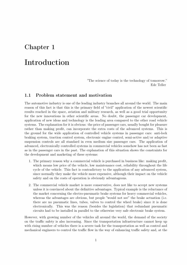
14

where Fmg is the magnetic force generated by the magnetic field of the solenoid, Frsp is the forcecoming from the return spring, F∆p is generated by the pressure difference on the cross section ofthe closed valve seat and Farm,lim is the stroke limiting force of the SMV armature. The forcesacting on the SMV armature can be seen in Fig. 2.3.

FmgFrspF∆pFarm,lim

x, v

Figure 2.3: Free body diagram of the solenoid magnet valve (SMV) armature

Since the SMV armature mass is constant in time according to A12, the equations for arma-ture velocity is obtained as:

dv

dt=Fmg − Frsp − F∆p − Farm,lim

m. (2.14)

The stroke change of the armature can be written as follows:

dx

dt= v. (2.15)

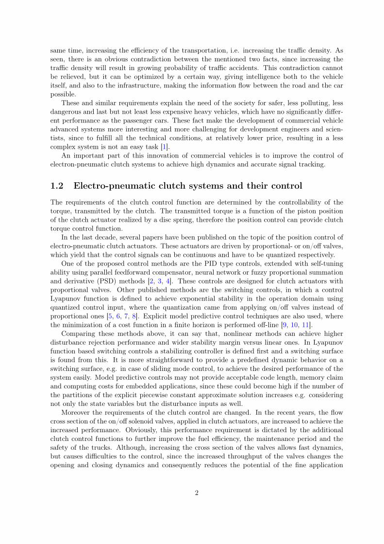
2.4.5 Conservation of magnetic linkage in the SMVs V9−10

The balance of the magnetic linkage is determined by Maxwell’s second equation (Faraday’s law),which describes how a time varying stand still magnetic field induces an electric field:

∮

CE dl = −

d

dt

∫

SB n da, (2.16)

where E is the electric field intensity, B is the magnetic flux density moreover the surface S isenclosed by the contour C and the positive direction of the normal vector n is defined by theusual right-hand rule (see Fig. 2.4).

n

B

Figure 2.4: Magnetic linkage in the solenoid

15

In regions, where the magnetic field is either static or negligible the electric field intensitycan be derived as the gradient of a scalar potential φ as follows:

E = −∇φ. (2.17)

The difference in potential between two points, say a and b, is a measure of the line integralof E, for

∫ b

aE dl =

∫ b

a−∇φ dl = φa − φb. (2.18)

The potential difference φa − φb is referred to as the voltage of point a with respect to b.Thus Faraday’s law yields the induced voltage (uind) of the solenoid as follows:

uind =d

dt

∫

SB n da =

dλ

dt=dλ

di

di

dt+dλ

dx

dx

dt, (2.19)

where λ is the flux linkage of the circuit.Assuming a magnetically linear system according to A7 whose flux linkage can be expressed

in terms of an inductance L as λ = L i. Through these the induced voltage becomes:

uind = Ldi

dt+ i

dL

dx

dx

dt. (2.20)

The terminal voltage of the SMVs (uterm) is dropped on the ohmic resistance (R) and theinductive parts as follows according to Kirchoff’s second law:

uterm = ures + uind. (2.21)

Using Ohm’s law and substitution of Eq. (2.20) into Eq. (2.21) the current change can be obtainedas follows:

di

dt=utermL

−R

Li−

1

L

dL

dx

dx

dti. (2.22)

2.5 Constitutive equations

To complete the above equations some additional algebraic constraints are needed to be definedsuch as transfer rates, property relations, equipment constraints and defining equations for othercharacterizing variables.

2.5.1 Chamber and gas properties

The volume of the chamber is obtained from a constant dead volume (V dch) and an additive

volume set by the moving piston of the system, where the dead volume of the chamber is definedas the minimum volume that the chamber may have, independent by of the current application.With these the chamber current volume of the clutch actuator can be written as follows:

Vch = V dch + xpstApst, (2.23)

where Apst is the cross section area of the piston.The volume change of the chamber is obtained as:

dVchdt

= vpstApst. (2.24)

16

The temperature of the gas in the chamber (Tch) is obtained using the ideal gas equation,thus the chamber gas temperature is written:

Tch =pchVchmchR

=pch(V dch + xpstApst

)

mchR. (2.25)

The heat transfer in the gas chamber is calculated according to Newton’s heat transfer law(see in assumption A4) that gives the following equation for the chamber:

Qch = khtAht(Tch − Tamb), (2.26)

where kht is the heat transfer coefficient and Aht is the surface area of the chamber.The work term can be calculated using the general gas work equation in case of changing

volume:

Wch = pchdVchdt

= pchvpstApst. (2.27)

2.5.2 SMV airflow properties

In general the local gas speed in the SMVs at vena contracta, the point in a flow, where thediameter of the flow is the least, is determined by the contraction coefficient (α) of the stream,the flow cross section (Ain), the source side- pressure (pin) and temperature (Tin) and the pressureratio (Π = pout/pin) between the in- and output ports [26] as follows:

σ = α Ain pin

√√√√ 2 κ

κ− 1

1

RTin

[(poutpin

) 2κ

−

(poutpin

)κ+1κ

]

. (2.28)

The flow cross section of the SMV is determined by its orifice between the valve seat andthe armature. If the armature stroke is less or equal to the value, where the armature reachesthe valve seat (xlim,1) see in Fig. 2.5, then there is no flow. If the stroke is above this value thesmallest orifice is determined by a cylindrical surface. If there is a big stroke then the orificeis limited by the area of the outlet hole. This implies hybrid behavior depending on the SMVarmature position.

Outlet port

Inlet port

Frame

Plug

Solenoid

Armature

Returnspring

m

x

v

x

xlim,2

lim,1

Seat

Figure 2.5: Two way two port on/off SMV layout

2.5.3 Forces acting on the piston

The force generated by the chamber pressure, acting on the piston surface and used to pre-stressthe disc spring, can be written as:

Fpch = (pch − pamb)Apst. (2.29)

17

The holder spring pushes the piston towards the disc spring, thus the holder spring forceacting on the piston can be written as follows:

Fhsp = chsp(xhsp0 − xpst), (2.30)

where chsp is the stiffness of the holder spring and xhsp0 is the spring pretension stroke.According to assumption A16 in which the clutch mechanism and the clutch actuator friction

effects are lumped together into one friction effect, the magnitude of the friction force (Ffr)depends on a lumped friction coefficient µpst and the piston pressure force. The actuator frictioncomes from the friction of the pressure amplified piston sealing. The friction of the clutchmechanism comes from the contact of the release bearing and the disc spring moreover thecontact of the disc spring and the pressure plate (see Fig. 2.1). The clamping forces of thesecontacts are also proportional with the pressure force. The friction force acts against the pistonmovement and introduces three hybrid items depending on the piston velocity.

Considering A17, in which assuming that the clutch mechanism and the clutch actuatordamping effects are lumped together into one damping effect kpst, the damping force actingagainst the piston movement is obtained as follows:

Fdmp = vpstkpst. (2.31)

The stroke limiting force (Fpst,lim) of the piston is modeled as a stiff spring if the strokeexceeds the limits. This introduces three hybrid modes, two limiting positions (xlim,1

pst and xlim,2pst )

at the stroke ends (see Fig. 2.1) and the third one corresponding to the intermediate position.The Fl(xpst), acting against the piston movement, comes from the clutch mechanism. This

force is a highly nonlinear function of the displacement, generated by the disc spring, the cushionsprings of the friction disc and the leaf springs. The explicit formula of the load characteristic(see Fig. 2.6), which can provide the prescribed accuracy, is too complex, therefore in the modela realization through the empirical center characteristic line will be used. The large hysteresis ofthe force characteristics, generated by the friction, is a result of the friction force defined above.

In accordance with assumption A19 the pretension of the disc spring does not change in spiteof the fact that the friction disc wears, hence the characteristic cannot change during the lifetimeof the clutch mechanism.

2.5.4 Forces acting on the SMV armature

The magnetic force (Fmg) can be calculated as the partial derivative of the energy of the magneticfield (E) with respect to the armature stroke as:

Fmg = −∂E

∂x= −

Θ2

2R2Σ

dRΣ

dx= −

(N i)2

2R2Σ

dRΣ

dx, (2.32)

where Θ is the excitation (magnetic voltage), RΣ is the magnetic resistance and N is the numberof solenoid turns.

The connected magnetic resistances are related to the frame (Rfrm), the plug (Rpl), theSMV armature (Rarm), the air clearance between the overlapping coaxial cylindrical surfacesof the SMV armature and the frame (Rc1) and finally resistance in the air clearance (Rc2(x))between the plug and the armature (see Fig. 2.5).

The only component that depends on the stroke is Rc2(x) and it is considered as follows:

Rc2(x) =xgap − x

µ0Aarm, (2.33)

18

0 2 4 6 8 10 12 14 16 18 20 220

1000

2000

3000

4000

5000

6000

7000

8000

9000

10000

xpst [mm]

Fl[N

]

Measurement dataCentre characteristic line

Figure 2.6: Characteristic of the clutch mechanism Fl (xpst)

where µ0 is the permeability of vacuum and Aarm = d2armπ/4 is the cross section of the SMVarmature body. Moreover xgap = xlim,2 − xlim,1 corresponds to the air clearance. The changeof Rarm is negligible small so it is considered constant as well. The magnetic resistance can becalculated as a function of armature stroke from the magnetic circuit as:

RΣ = Rpl +Rfrm +Rc1 +Rc2(x) +Rarm. (2.34)

The constant part of RΣ is denoted by R as the constant part of the magnetic loop so the totalmagnetic resistance can be given as:

RΣ = R−x

µ0Aarm. (2.35)

Since there is only one stroke dependent component, the derivative function with respect to x iswritten as:

dRΣ

dx=dRc2(x)

dx= −

1

µ0Aarm. (2.36)

With this the magnetic force can be expressed as follows:

Fmg =(N i)2

2(

R− xµ0Aarm

)2

1

µ0Aarm. (2.37)

The force coming from the armature return spring is obtained as follows:

Frsp = srsp (x+ xrsp0) + krspv, (2.38)

where srsp is the stiffness, xrsp0 is the pretension and krsp is the damping of the return spring.

19

The force on the armature generated by the difference pressure (F∆p) introduces two hybridmodes for each SMV. In case of closed valve the difference pressure force is generated by thepressure difference between the input and output port of the valve acting on the cross section asfollows:

F∆p =d2π

4(pin − pout). (2.39)

Otherwise this force is equal to zero in accordance with A10.Similarly to the piston stroke limitation the SMV armature stroke limiting force (Farm,lim)

is modeled as a stiff spring if the stroke exceeds the limits (xlim,1 and xlim,2). This introducesthree more hybrid modes for each SMV the same way as it already been discussed.

2.5.5 Electro-magnetic relations

The inductance of the SMV is written as the following equality of the number of solenoid turnsand the magnetic resistance:

L =N2

RΣ. (2.40)

Its derivative with respect to the armature position can be written as:

dL

dx=

dL

dRΣ

dRΣ

dx(2.41)

and derivative with respect to the magnetic resistance is given as follows:

dL

dRΣ= −

N2

R2Σ

. (2.42)

2.5.6 Power stage relations

The electric circuits of the SMVs (see Fig. 2.1) are low side driven, this means that one of theterminals of the SMVs is connected to the supply voltage (Usup) and the other is connected tothe switching element of the power stage. The power stages are driven by the clutch controlunit with high frequency PWM signals (uin). In accordance with assumption A13 the PWMfrequency is high enough to approximate the currents with its average values, thus the terminalvoltage of the SMVs depends only on the supply voltage and on the voltage drop of the powerstage (upws) as follows:

uterm = Usup − upws. (2.43)

The voltage drop of the power stages introduce three hybrid states depending on whetherthe duty cycle (md) of the PWM signal and the SMV current are equal or greater than zero.This is the consequence of the unclamped switching [27]. As the SMVs are switched off a highinduced voltage appears between the terminals of the SMVs, due to the self inductance, whichare limited by the power stage.

Hence the voltage drop of the power stages can be written as follows:

upws =

Usup (1−md) + rDS(on) · i, if md > 0

UBR, if md = 0 and i > 0

Usup, otherwise,

(2.44)

where UBR is the breakdown voltage of the MOSFET and rDS(on) is the drain to source turnedon resistance according to Assumption A14.

20

2.6 Hybrid items

To generalize the model all of the cases that describe the changes in the conservation and con-stitutive equations of the model have to be collected.

The model includes five model element types that exhibit discrete-continuous behavior. Thefirst is the voltage drop of the power stages marked with HM1−4,x for the four SMVs. The nextis the air flow term of the SMVs, the related hybrid modes marked with HM5,x and HM6,x forload and exhaust SMVs respectively. The third is the flow cross-section, difference pressure forceand armature stroke limiting force of the SMVs, marked with HM7−10,x for the four SMVs. Thefourth term is the piston stroke limiting force HM11,x and the last is the friction force of thepiston HM12,x.

2.6.1 Power stage voltage drop

The power stage of the SMVs can be considered as a switching element which inherently causeshybrid behavior. Moreover the unclamped inductive switching, where the power stage itselflimits the induced voltage in the avalanche state, introduces three hybrid states according to theduty cycle of the control PWM signal and the solenoid current weather they are equal or graterthan zero. In this way the three states are as follows: switched on state, after switch of state(avalanche) and released state. The corresponding hybrid modes are shown in Tab. 2.2.

Table 2.2: Hybrid modes of the power stage voltage drop

No. Condition upws

HM1−4,1 md > 0 Usup (1−md) + rDS(on) · i

HM1−4,2 md = 0 and i > 0 UBR

HM1−4,3 md = 0 and i = 0 Usup

2.6.2 SMV airflow term

The air flow on a port between two chambers (see Eq. (2.28)) is governed by the pressure ratio(Π). In connection with the flow, four cases can be distinguished that can be subsonic and sonicin both directions (assuming that no Laval geometry is met). The sonic flow conditions aredetermined by the critical pressure ratio as:

Πcrit =

(2

κ+ 1

) κκ−1

. (2.45)

Assumption A6 states that the SMVs air flow have non-negative values only. This impliesonly two hybrid modes in the same flow direction. So there is only one part in Eq. (2.28) thatdepends on the hybrid mode, namely the pressure ratio under the exponents. The correspondinghybrid modes are shown in Tab. 2.3.

2.6.3 Armature stroke dependent terms of the valves

The flow cross section expressions, the pressure difference- and stroke limiting forces are depend-ing on the armature stroke of the SMVs, in this way they are dependent hybrid modes regardingto the same SMV.

Assumption A8 considers that the armature stroke can be bigger than d/4, which impliesthree hybrid modes regarding to the flow cross section such as zero-, cylindrical- and circular

21

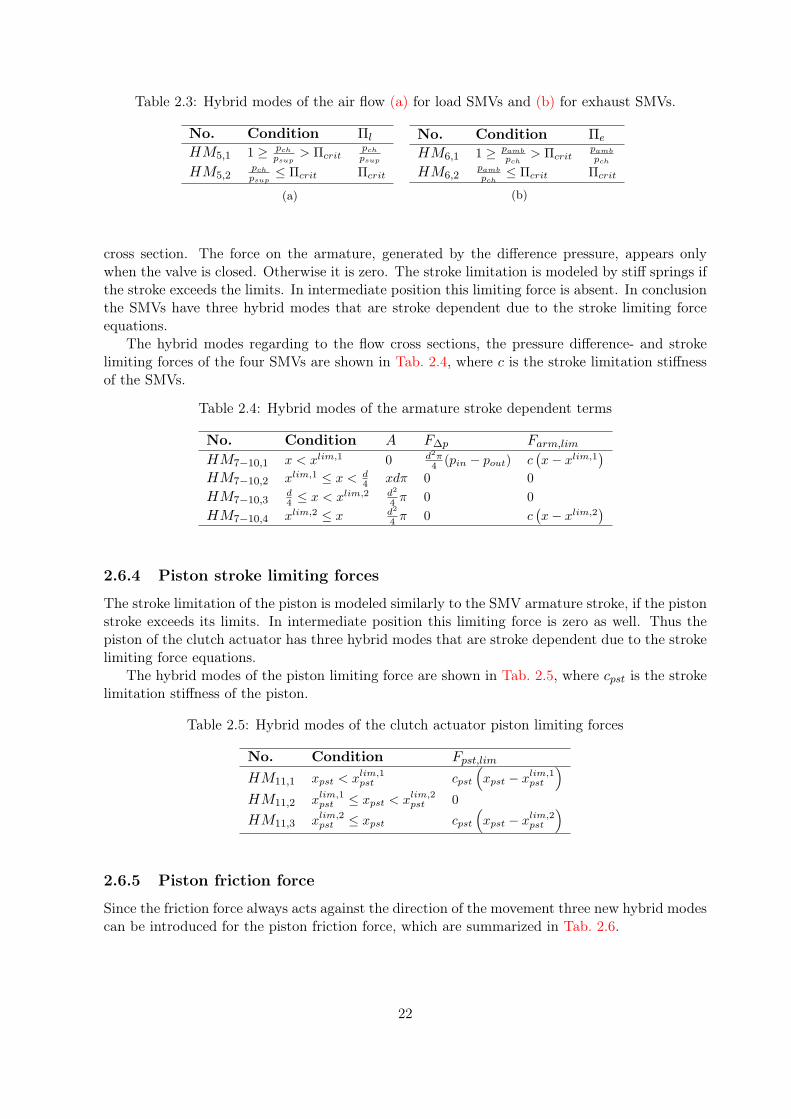
Table 2.3: Hybrid modes of the air flow (a) for load SMVs and (b) for exhaust SMVs.

No. Condition Πl

HM5,1 1 ≥ pch

psup> Πcrit

pch

psup

HM5,2pch

psup≤ Πcrit Πcrit

(a)

No. Condition Πe

HM6,1 1 ≥ pamb

pch> Πcrit

pamb

pch

HM6,2pamb

pch≤ Πcrit Πcrit

(b)

cross section. The force on the armature, generated by the difference pressure, appears onlywhen the valve is closed. Otherwise it is zero. The stroke limitation is modeled by stiff springs ifthe stroke exceeds the limits. In intermediate position this limiting force is absent. In conclusionthe SMVs have three hybrid modes that are stroke dependent due to the stroke limiting forceequations.

The hybrid modes regarding to the flow cross sections, the pressure difference- and strokelimiting forces of the four SMVs are shown in Tab. 2.4, where c is the stroke limitation stiffnessof the SMVs.

Table 2.4: Hybrid modes of the armature stroke dependent terms

No. Condition A F∆p Farm,lim

HM7−10,1 x < xlim,1 0 d2π4 (pin − pout) c

(x− xlim,1

)

HM7−10,2 xlim,1 ≤ x < d4 xdπ 0 0

HM7−10,3d4 ≤ x < xlim,2 d2

4 π 0 0

HM7−10,4 xlim,2 ≤ x d2

4 π 0 c(x− xlim,2

)

2.6.4 Piston stroke limiting forces

The stroke limitation of the piston is modeled similarly to the SMV armature stroke, if the pistonstroke exceeds its limits. In intermediate position this limiting force is zero as well. Thus thepiston of the clutch actuator has three hybrid modes that are stroke dependent due to the strokelimiting force equations.

The hybrid modes of the piston limiting force are shown in Tab. 2.5, where cpst is the strokelimitation stiffness of the piston.

Table 2.5: Hybrid modes of the clutch actuator piston limiting forces

No. Condition Fpst,lim

HM11,1 xpst < xlim,1pst cpst

(

xpst − xlim,1pst

)

HM11,2 xlim,1pst ≤ xpst < xlim,2

pst 0

HM11,3 xlim,2pst ≤ xpst cpst

(

xpst − xlim,2pst

)

2.6.5 Piston friction force

Since the friction force always acts against the direction of the movement three new hybrid modescan be introduced for the piston friction force, which are summarized in Tab. 2.6.

22

Table 2.6: Hybrid modes of the Friction forces

No. Condition Ffr

HM12,1 vpst < 0 −µpst (pch − pamb)Apst

HM12,2 vpst = 0 0

HM12,3 vpst > 0 µpst (pch − pamb)Apst

2.7 Model equations in state space form

One of the most widespread model representation for analysis and control design purposes isthe state space realization based on a set of coupled first-order differential algebraic equationsincluding a set of system variables in vector format [28]. Since this realization is not unique,many equivalent representations with the same dimension can be found, giving rise to the sameinput-output description of a given system.

Hence for the EPC model the following system variables are composed to retain the physicalmeaning of the variables. In order to distinguish the equations of the four SMVs the correspondingindices are used for their variables and parameters.

From the conservation equations the state vector is composed of their differential variablesas follows:

x = [ isl vsl xsl ibl vbl xbl ise vse xse ibe vbe xbe mch pch vpst xpst ]T . (2.46)

The uncontrollable inputs form the disturbance vector including the supply voltage, compressed(supply) air- pressure and temperature, ambient- pressure and temperature respectively:

d =[Usup psup Tsup pamb Tamb

]T. (2.47)

The control input vector includes the duty cycle of the PWM control signals:

u =[md,sl md,bl md,se md,be

]T. (2.48)

The measurable state variables and disturbances are formed as measured output including thecurrent of the SMVs, the chamber pressure, the piston position, the supply voltage and thesupply pressure:

y =[isl ibl ise ibe pch xpst Usup psup

]T. (2.49)

2.7.1 State equations

The following hybrid nonlinear state space form [29] of the DAEs of the model is considered:

dx(k)M0

dt= f

(k)M0

(

x(k)M0

, u(k)M0

, d(k)M0

)

, (2.50)

where k : Rn → N is a piece-wise constant switching function mapping from the state space toN. The integer set N is finite, i.e. N = 1, 2, . . . , n, where n =

∏12i=1 ni is the total number of

hybrid modes and ni is the number of the individual hybrid modes of a model element (n =3 × 3 × 3 × 3 × 2 × 2 × 4 × 4 × 4 × 4 × 3 × 3 = 746496). Moreover, the values of k can becomposed by the conditions defined in Tab. 2.2-2.6. The nonlinear state functions are written

23

as (the entries that depend on the hybrid modes are boxed, the meaning of the parameters canbe found in Tab. A.1 and the meaning of the variables can be found in the Nomenclature):

f(k)1,M0

= −vsl isl

(

Rsl −xsl

µ0 Aarmsl

)

µ0Aarmsl

+

(

Rsl −xsl

µ0 Aarmsl

)(

Usup −Rsl isl − upwssl

)

Nsl2 , (2.51)

f(k)2,M0

=

(Nsl isl)2

2

(

Rsl−xsl

µ0 Aarmsl

)21

µ0 Aarmsl

msl−ssl (xsl + xsl,0) + ksl vsl + F∆p,sl + F lim

sl

msl, (2.52)

f(k)3,M0

= vsl, (2.53)

f(k)4,M0

= −vbl ibl

(

Rbl −xbl

µ0 Aarmbl

)

µ0Aarmbl

+

(

Rbl −xbl

µ0 Aarmbl

)(

Usup −Rbl ibl − upwsbl

)

Nbl2 , (2.54)

f(k)5,M0

=

(Nbl ibl)2

2

(

Rbl−xbl

µ0 Aarmbl

)21

µ0 Aarmbl

mbl−sbl (xbl + xbl,0) + kbl vbl + F∆p,bl + F lim

bl

mbl, (2.55)

f(k)6,M0

= vbl, (2.56)

f(k)7,M0

= −vse ise

(

Rse −xse

µ0 Aarmse

)

µ0Aarmse

+

(

Rse −xse

µ0 Aarmse

)(

Usup −Rse ise − upwsse

)

Nse2 , (2.57)

f(k)8,M0

=

(Nse ise)2

2(

Rse−xse

µ0 Aarmse

)21

µ0 Aarmse

mse−sse (xse + xse,0) + kse vse + F∆p,se + F lim

se

mse, (2.58)

f(k)9,M0

= vse, (2.59)

f(k)10,M0

= −vbe ibe

(

Rbe −xbe

µ0 Aarmbe

)

µ0Aarmbe

+

(

Rbe −xbe

µ0 Aarmbe

)(

Usup −Rbe ibe − upwsbe

)

Nbe2 , (2.60)

f(k)11,M0

=

(Nbe ibe)2

2

(

Rbe−xbe

µ0 Aarmbe

)21

µ0 Aarmbe

mbe−sbe (xbe + xbe,0) + kbe vbe + F∆p,be + F lim

be

mbe, (2.61)

24

f(k)12,M0

= vbe, (2.62)

f(k)13,M0

=(

αsl Asl + αbl Abl

)

ξl −(

αse Ase + αbe Abe

)

ξe , (2.63)

f(k)14,M0

=κR

(

αsl Asl + αbl Abl

)

ξl Tsup

V dch + xpstApst

−κ pch

(

αse Ase + αbe Abe

)

ξe

mch−

−

(κ− 1) khtAht

(pch(V d

ch+xpstApst)mchR

− Tamb

)

V dch + xpstApst

−κ pch vpstApst

V dch + xpstApst

, (2.64)

f(k)15,M0

=(pch − pamb)Apst + shsp(xhsp0 − xpst)

mpst−

Ffr + vpstkpst + F limpst + Fl(xpst)

mpst, (2.65)

f(k)16,M0

= vpst, (2.66)

where

ξl =

√

2 κ

κ− 1

p2supRTsup

(

Πl

2κ − Πl

κ+1κ

)

and (2.67)

ξe =

√

2 κ

κ− 1

pchmch(V dch + xpstApst

)

(

Πe

2κ − Πe

κ+1κ

)

. (2.68)

2.7.2 Output equations

Since the output is linear with respect to the state vector, the measured output is written as thefollowing equation:

yM0= CM0

xM0+EM0

dM0, (2.69)

where the matrix CM0is determined by the intended application of the model, e.g. on purpose

to do simulations for verification CM0can be equal to the identity matrix to reach all the state

variables. As opposed to the simulation the instrumental conditions do not make it possibleto reach all the state variables thus for validation purposes the model output matrix has beenselected as the following way CM0

=< ci,j >, where c1,1 = c2,4 = c3,7 = c4,10 = c5,14 = c6,16 = 1and the remained elements are equal to zero:

CM0=

1 0 0 0 0 0 0 0 0 0 0 0 0 0 0 00 0 0 1 0 0 0 0 0 0 0 0 0 0 0 00 0 0 0 0 0 1 0 0 0 0 0 0 0 0 00 0 0 0 0 0 0 0 0 1 0 0 0 0 0 00 0 0 0 0 0 0 0 0 0 0 0 0 1 0 00 0 0 0 0 0 0 0 0 0 0 0 0 0 0 10 0 0 0 0 0 0 0 0 0 0 0 0 0 0 00 0 0 0 0 0 0 0 0 0 0 0 0 0 0 0

. (2.70)

25

The matrix EM0corresponds to the measured disturbances which are the Usup and psup,

hence it is written as follows:

EM0=

0 0 0 0 00 0 0 0 00 0 0 0 00 0 0 0 00 0 0 0 00 0 0 0 01 0 0 0 00 1 0 0 0

. (2.71)

The performance output is generated from the measured output by the following simpleequation:

zM0= [ 0 0 0 0 0 1 0 0 ]yM0

. (2.72)

2.8 Model verification and validation

The verification of the developed model is performed by extensive simulations usingMATLAB/SIMULINK model. The simulation results are compared to the real system behaviorsuch as trends-, operation domain- and relationship of the variables. These attributes above aregathered from operation experiences on the real system. To obtain the model solutions the stiffODE15s solver, with variable step size has been used, where the relative tolerance of the solverhas been set up to 10−8.

In the simulation calculations two typical operating cases have been considered. One of themhas been executed with load SMVs excitations only in order to see the activation effect of thesevalves on the chamber pressure. In this operating case, called disengagement, the pressure forceloads the disc spring, hence the pressure plate can separate from the friction disc. In the otherthe exhaust SMVs excitations have been investigated in order to see the activation effect of theexhaust SMVs on the chamber pressure. This operating case, when the pressure is decreased inthe chamber, is used for the engagement of the clutch.

The parameters, considered in simulation calculations, can be seen in Appendix A in Tab. A.1.The model parameters can be divided into three groups according to the knowledge and confi-dence of their values as known-, partially known and unknown parameters. Known parametersare physical constants from the thermo- and electro-dynamics and have well defined values. Par-tially known parameters are pre-specified or can be measured independently of the system bysimple, usually static methods. The unknown parameters should be identified using experimen-tal data from the real process. Because measured data contain measurement errors, the missingmodel parameters can only be estimated.

In [30] an electro-pneumatic protection valve model has been identified and it has beenfound that the unknown parameters, for which the model sensitivity is high, are the contractioncoefficients and the magnetic resistances of the SMVs. Hence, based on this result similar valuesare considered for these model parameters.

2.8.1 Disengagement process verification

This process has been simulated with constant disturbances, starting from the engaged state ofthe clutch mechanism (currentless valves and exhausted chamber). The initial state vector is as

26

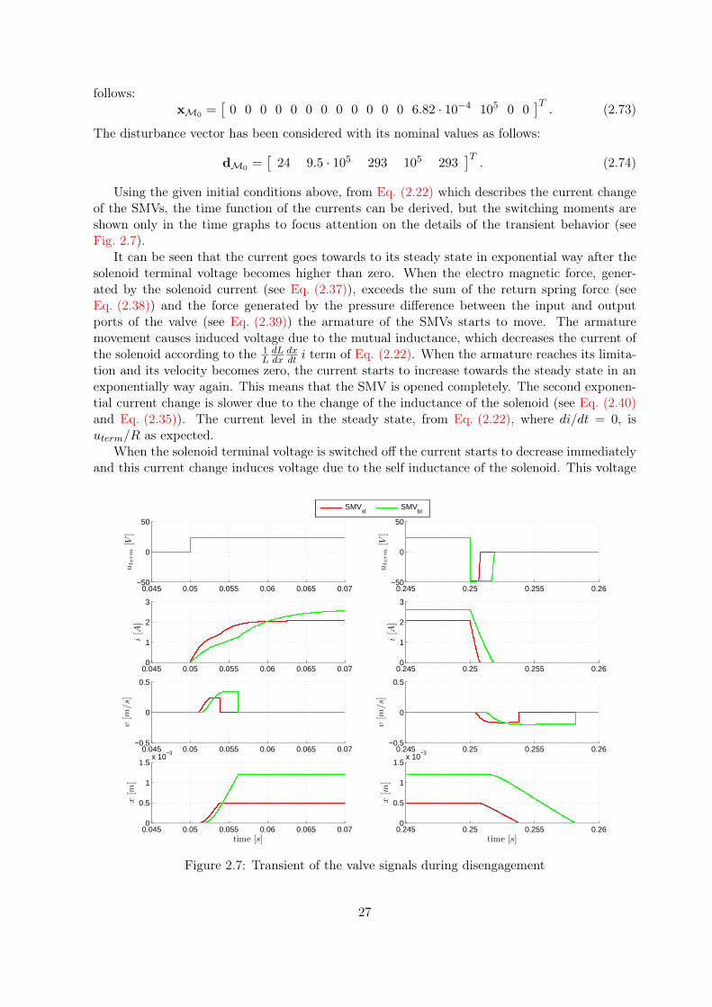
follows:xM0

=[0 0 0 0 0 0 0 0 0 0 0 0 6.82 · 10−4 105 0 0

]T. (2.73)

The disturbance vector has been considered with its nominal values as follows:

dM0=[24 9.5 · 105 293 105 293

]T. (2.74)

Using the given initial conditions above, from Eq. (2.22) which describes the current changeof the SMVs, the time function of the currents can be derived, but the switching moments areshown only in the time graphs to focus attention on the details of the transient behavior (seeFig. 2.7).

It can be seen that the current goes towards to its steady state in exponential way after thesolenoid terminal voltage becomes higher than zero. When the electro magnetic force, gener-ated by the solenoid current (see Eq. (2.37)), exceeds the sum of the return spring force (seeEq. (2.38)) and the force generated by the pressure difference between the input and outputports of the valve (see Eq. (2.39)) the armature of the SMVs starts to move. The armaturemovement causes induced voltage due to the mutual inductance, which decreases the current ofthe solenoid according to the 1

LdLdx

dxdt i term of Eq. (2.22). When the armature reaches its limita-

tion and its velocity becomes zero, the current starts to increase towards the steady state in anexponentially way again. This means that the SMV is opened completely. The second exponen-tial current change is slower due to the change of the inductance of the solenoid (see Eq. (2.40)and Eq. (2.35)). The current level in the steady state, from Eq. (2.22), where di/dt = 0, isuterm/R as expected.

When the solenoid terminal voltage is switched off the current starts to decrease immediatelyand this current change induces voltage due to the self inductance of the solenoid. This voltage

0.045 0.05 0.055 0.06 0.065 0.07−50

0

50

uterm

[V]

0.245 0.25 0.255 0.26−50

0

50

uterm

[V]

0.045 0.05 0.055 0.06 0.065 0.070

1

2

3

i[A

]

0.245 0.25 0.255 0.260

1

2

3

i[A

]

0.045 0.05 0.055 0.06 0.065 0.07−0.5

0

0.5

v[m

/s]

0.245 0.25 0.255 0.26−0.5

0

0.5

v[m

/s]

0.045 0.05 0.055 0.06 0.065 0.070

0.5

1

1.5x 10

−3

x[m

]

time [s]0.245 0.25 0.255 0.260

0.5

1

1.5x 10

−3

x[m

]

time [s]

SMVsl

SMVbl

Figure 2.7: Transient of the valve signals during disengagement

27

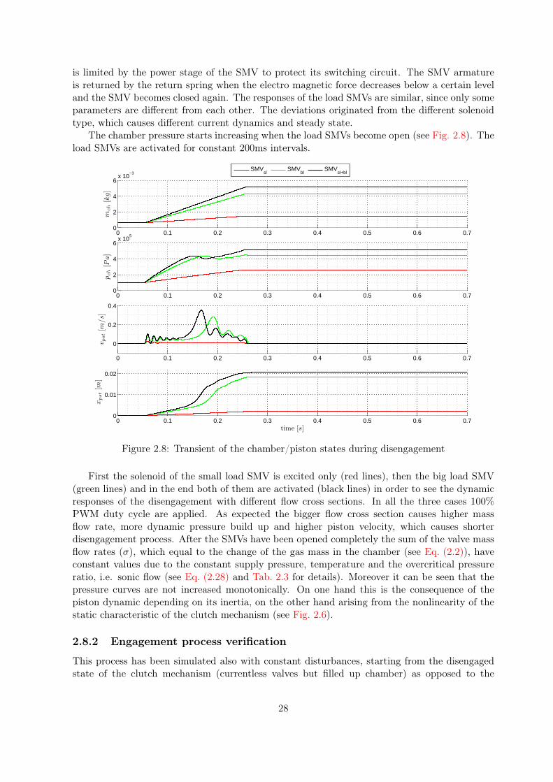
is limited by the power stage of the SMV to protect its switching circuit. The SMV armatureis returned by the return spring when the electro magnetic force decreases below a certain leveland the SMV becomes closed again. The responses of the load SMVs are similar, since only someparameters are different from each other. The deviations originated from the different solenoidtype, which causes different current dynamics and steady state.

The chamber pressure starts increasing when the load SMVs become open (see Fig. 2.8). Theload SMVs are activated for constant 200ms intervals.

0 0.1 0.2 0.3 0.4 0.5 0.6 0.70

2

4

6x 10

−3

mch

[kg]

0 0.1 0.2 0.3 0.4 0.5 0.6 0.70

2

4

6x 10

5

pch

[Pa]

0 0.1 0.2 0.3 0.4 0.5 0.6 0.7

0

0.2

0.4

v pst

[m/s]

0 0.1 0.2 0.3 0.4 0.5 0.6 0.70

0.01

0.02

xpst

[m]

time [s]

SMVsl

SMVbl

SMVsl+bl

Figure 2.8: Transient of the chamber/piston states during disengagement

First the solenoid of the small load SMV is excited only (red lines), then the big load SMV(green lines) and in the end both of them are activated (black lines) in order to see the dynamicresponses of the disengagement with different flow cross sections. In all the three cases 100%PWM duty cycle are applied. As expected the bigger flow cross section causes higher massflow rate, more dynamic pressure build up and higher piston velocity, which causes shorterdisengagement process. After the SMVs have been opened completely the sum of the valve massflow rates (σ), which equal to the change of the gas mass in the chamber (see Eq. (2.2)), haveconstant values due to the constant supply pressure, temperature and the overcritical pressureratio, i.e. sonic flow (see Eq. (2.28) and Tab. 2.3 for details). Moreover it can be seen that thepressure curves are not increased monotonically. On one hand this is the consequence of thepiston dynamic depending on its inertia, on the other hand arising from the nonlinearity of thestatic characteristic of the clutch mechanism (see Fig. 2.6).

2.8.2 Engagement process verification

This process has been simulated also with constant disturbances, starting from the disengagedstate of the clutch mechanism (currentless valves but filled up chamber) as opposed to the

28

previous case. The initial state vector is as:

xM0=[0 0 0 0 0 0 0 0 0 0 0 0 43.93 · 10−4 4 · 105 0 15.43 · 10−3

]T. (2.75)

The disturbance vector is considered to be the same as before.The responses of the exhaust and load SMVs are similar to each other (see Fig. 2.9).

0.045 0.05 0.055 0.06 0.065 0.07−50

0

50

uterm

[V]

0.845 0.85 0.855 0.86−50

0

50

uterm

[V]

0.045 0.05 0.055 0.06 0.065 0.070

1

2

3

i[A

]

0.845 0.85 0.855 0.860

1

2

3

i[A

]

0.045 0.05 0.055 0.06 0.065 0.07−0.5

0

0.5

v[m

/s]

0.845 0.85 0.855 0.86−0.5

0

0.5v

[m/s]

0.045 0.05 0.055 0.06 0.065 0.070

0.5

1

1.5x 10

−3

x[m

]

time [s]0.845 0.85 0.855 0.860

0.5

1

1.5x 10

−3

x[m

]

time [s]

SMVse

SMVbe

Figure 2.9: Transient of the valve signals during engagement

As expected, the chamber pressure starts to decrease when the exhaust SMVs become open(see Fig. 2.10). The exhaust SMVs are activated for constant 800ms intervals and for all thecases 100% PWM duty cycle has been applied. First the solenoid of the small exhaust SMV isexcited (blue lines), then the big exhaust SMV (magenta lines) and in the end both of them areactivated (black lines) in order to see the dynamic responses of the engagement with differentflow cross sections similarly as before.

Although the flow cross sections of the load and exhaust valves are equal, the engagementprocesses show slower dynamic piston movement compared to the disengagement, caused by theavailable mass flow rate. This is influenced by the pressure ratio differences (see Eq. (2.28))between the ambient-chamber and chamber-reservoir pressures. The pressure curves do notchange in a monotonic way, similarly to the disengagement process, due to compression effects.

2.8.3 Validation

In order to validate the model, the model output vector has been compared to measurements onthe real EPC system. The measurement set-up includes a measurement PC with data acquisitionunit that is connected to the measurement sensors. The data acquisition unit is able to measureanalogue-to-digital converted (ADC) channels and has digital I/O channels that can be used as

29

0 0.2 0.4 0.6 0.8 1 1.2 1.40

2

4

6x 10

−3

mch

[kg]

0 0.2 0.4 0.6 0.8 1 1.2 1.41

2

3

4

5x 10

5

pch

[Pa]

0 0.2 0.4 0.6 0.8 1 1.2 1.4−0.4

−0.2

0

v pst

[m/s]

0 0.2 0.4 0.6 0.8 1 1.2 1.40

0.01

0.02

xpst

[m]

time [s]

SMVse

SMVbe

SMVse+be

Figure 2.10: Transient of the chamber/piston states during engagement

control outputs to switching the power stages of the SMVs properly. The resolution of the ADCchannels is 14 bits and the sampling frequency can be set up to 20kHz.

The target is to control the real system by its input vector to execute predefined test sequencesand to measure all the characterizing signals which are available. Hence, all the members of theinput and the output vector are measured on the test bench, which introduces ten signals tothe measurement system that are as follows: uterm,sl, uterm,bl, uterm,se, uterm,be, isl, ibl, ise, ibe,pch and xpst. Note that, instead of the real inputs (md) the terminal voltage of the SMVs aremeasured, since they represent not only the presence or absence of the supply voltage betweenthe terminals of the SMVs but also show the brake down voltage (UBR) in the avalanche state.

To predict the behavior of the real system the disturbance variables should be known as well.From the five signals of the disturbance vector three can be considered as quasi-constant signals(Tsup, pamb and Tabm) that changes slowly, so these values are assumed to be constants (293K,105Pa and 293K). The remained (usup and psup) can change dynamically, so they should beacquired as well. The accuracy and the measurement range, according to the specification of thesensor suppliers, are seen in Tab. 2.7.

Table 2.7: Accuracy and range of measured signals

Signal u [V] i [A] p [Pa] x [m]

minima -60 0 0 0maxima 40 4 16× 105 0.04accuracy [%] ±1 ±1 ±1.6 ±2

For validation purpose the simulated test cases above are acquired on a real EPC bench. Thenan additional test case has been acquired that includes a real clutching procedure. Through these

30

the first six test cases investigate short term dynamic behavior with one excitation of differentSMV combination. The seventh one checks the long term dynamics with SMV excitation for areal clutching procedure.

The disengagement and engagement with various SMV combinations are presented below.The measured and the simulated signals are represented with continuous- and dashed lines re-spectively. The transient states of the SMVs in the switching moment are shown in see Fig. 2.11and Fig. 2.12.

0.045 0.05 0.055 0.06−50

−40

−30

−20

−10

0

10

20

30

uterm

[V]

SMVsl on

0.045 0.05 0.055 0.060

0.5

1

1.5

2

2.5

3

i[A

]

time [s]

0.248 0.25 0.252 0.254 0.256

SMVsl off

0.248 0.25 0.252 0.254 0.256time [s]

0.395 0.4 0.405 0.41

SMVbl

on

0.395 0.4 0.405 0.41time [s]

0.598 0.6 0.602 0.604 0.606

SMVbl

off

0.598 0.6 0.602 0.604 0.606time [s]

SMVmessl

SMVsimsl

SMVmesbl

SMVsimbl

SMVmesse

SMVsimse

SMVmesbe

SMVsimbe

Figure 2.11: Transient of the terminal voltages and currents during disengagement

The deviations in the SMV currents between the measurement and simulation caused by thesimplifying assumptions, in which the nonlinearity and the dynamics of the SMVs are neglectedand reduced respectively (see Assumptions A7, A10 and A11). In spite of the deviations betweenthe simulated and the measured currents in opening direction the valve opening times are closeto each other. This can be seen from the change of the current curve, as it has been described inthe verification above, where the armature of the valve reaches its stroke limit i.e. opened fully.In closing direction the currents have no major deviations, thus the closing times are close toeach other as well. The remained assumptions related to the model of the SMVs (AssumptionsA6, A12) have no significant influence on the SMV model accuracy. Since the resulted openingand closing time differences between the measurement and simulation have small impact on theremained part of the system, the simplification assumptions for the SMVs can be accepted.

In the next two graphs the pressure and the position signals are presented (see Fig. 2.13 andFig. 2.14).

The deviations between the measured and simulated pressure and piston position signals arecaused mainly by the simplifying assumptions (Assumption A18) in which, the clutch nonlinearforce characteristics is approximated with its empirical centre curve. The remained assumptionsfor the clutch mechanism (Assumption A15-A17 and A19) have no significant effect on the

31

1.095 1.1 1.105 1.11−50

−40

−30

−20

−10

0

10

20

30

uterm

[V]

SMVse

on

1.095 1.1 1.105 1.110

0.5

1

1.5

2

2.5

3

i[A

]

time [s]

1.898 1.9 1.902 1.904

SMVse

off

1.898 1.9 1.902 1.904time [s]

2.1 2.105 2.11

SMVbe

on

2.1 2.105 2.11time [s]

2.898 2.9 2.902 2.904 2.906

SMVbe

off

2.898 2.9 2.902 2.904 2.906time [s]

SMVmessl

SMVsimsl

SMVmesbl

SMVsimbl

SMVmesse

SMVsimse

SMVmesbe

SMVsimbe

Figure 2.12: Transient of the terminal voltages and currents during engagement

0 0.05 0.1 0.15 0.2 0.25 0.30

1

2

3

4

5

x 105

pch

[Pa]

0 0.05 0.1 0.15 0.2 0.25 0.30

0.005

0.01

0.015

0.02

xpst

[m]

time [s]

SMVmessl

SMVsimsl

SMVmesbl

SMVsimbl

SMVmessl+bl

SMVsimsl+bl

Figure 2.13: Transient of the pressure and position during disengagement

32

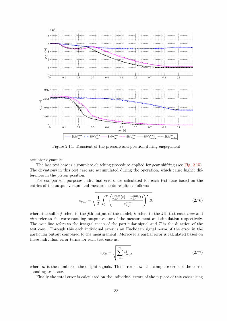
0 0.1 0.2 0.3 0.4 0.5 0.6 0.7 0.8 0.90

1

2

3

4

5

x 105

pch

[Pa]

0 0.1 0.2 0.3 0.4 0.5 0.6 0.7 0.8 0.90

0.005

0.01

0.015

0.02

xpst

[m]

time [s]

SMVmesse

SMVsimse

SMVmesbe

SMVsimbe

SMVmesse+be

SMVsimse+be

Figure 2.14: Transient of the pressure and position during engagement

actuator dynamics.The last test case is a complete clutching procedure applied for gear shifting (see Fig. 2.15).

The deviations in this test case are accumulated during the operation, which cause higher dif-ferences in the piston position.

For comparison purposes individual errors are calculated for each test case based on theentries of the output vectors and measurements results as follows:

ǫyk,j =

√√√√ 1

T

∫ T

0

(

ymesk,j (t)− ysimk,j (t)

ymesk,j

)2

dt, (2.76)

where the suffix j refers to the jth output of the model, k refers to the kth test case, mes andsim refer to the corresponding output vector of the measurement and simulation respectively.The over line refers to the integral mean of the particular signal and T is the duration of thetest case. Through this each individual error is an Euclidean signal norm of the error in theparticular output compared to the measurement. Moreover a partial error is calculated based onthese individual error terms for each test case as:

ǫP,k =

√√√√

m∑

j=1

ǫ2yk,j , (2.77)

where m is the number of the output signals. This error shows the complete error of the corre-sponding test case.

Finally the total error is calculated on the individual errors of the n piece of test cases using

33

0 0.2 0.4 0.6 0.8 1 1.2 1.4 1.6−50

0

50

uterm

[V]

0 0.2 0.4 0.6 0.8 1 1.2 1.4 1.60

1

2

3

i[A

]

SMVmessl

SMVsimsl

SMVmesbl

SMVsimbl

SMVmesse

SMVsimse

SMVmesbe

SMVsimbe

0 0.2 0.4 0.6 0.8 1 1.2 1.4 1.60

2

4

x 105

pch

[Pa]

pmes

ch psimch

0 0.2 0.4 0.6 0.8 1 1.2 1.4 1.60

0.005

0.01

xpst

[m]

time [s]

xmes

pst xsimpst

Figure 2.15: Real clutching procedure in case of gear shifting

the squared mean as follows:

ǫT =

√√√√

1

n

n∑

k=1

ǫ2P,k. (2.78)

Analyzing the individual errors (see Tab. 2.8), in the test case 1-6, it can be seen that thesmall SMVs have smaller current deviations than the big ones, moreover the big load SMV haslarger current deviations than the big exhaust SMV i.e.

ǫy1,1 ≈ ǫy3,1 ≈ ǫy4,3 ≈ ǫy6,3 < ǫy5,4 ≈ ǫy6,4 < ǫy2,2 ≈ ǫy3,2 (2.79)

It is the consequence of the unmodeled nonlinear magnetic behavior of the SMV material, whichnonlinearity depends on the magnitude of the applied current [31]. The magnitude distributionof the current deviations, in the seventh test case, is different. In this test case the deviationsdistribution has a relation with the switching number of the SMVs, since the steady state currenterrors are small.

Moreover the deviations between the measured and simulated pressure and position signals,on one hand, are caused by the SMV model deviations, on the other hand, are caused bythe reduced dynamics of the gas energy and the reduced dynamics of the piston momentum.Nevertheless, the total error in the validation is below the specified tolerance limit, thus themodel accuracy can be accepted, χMP5a-g are satisfied.

2.9 Summary

The multi-physical nature of the EPC is considered as a mixed thermodynamic, electro-magneticand mechanical system. The model of this system has been built and verified using a system-

34

Table 2.8: The modeling errors in case of nonlinear dynamic hybrid model

k Test case ǫyk,1[%] ǫyk,2

[%] ǫyk,3[%] ǫyk,4

[%] ǫyk,5[%] ǫyk,6

[%] ǫP[%] ǫT[%]

1 Diseng. 1 1.88 0.03 0.06 0.04 1.80 0.76 2.712 Diseng. 2 0.06 3.84 0.06 0.04 2.46 3.00 5.453 Diseng. 3 1.88 3.78 0.06 0.04 2.98 2.71 5.844 Eng. 1 0.06 0.03 1.58 0.04 0.78 1.16 2.11 4.32

5 Eng. 2 0.06 0.03 0.09 2.81 1.07 1.15 3.216 Eng. 3 0.06 0.03 1.83 2.45 0.83 1.09 3.357 Clutching 1.02 1.72 3.31 3.80 1.47 1.38 5.78

< χMP5a < χMP5b < χMP5c < χMP5d < χMP5e < χMP5f < χMP5g

atic modeling methodology. Moreover the effects of the simplifying assumptions on the model-accuracy and on the behavior have been verified and validated.

The model can be classified as a mechanistic, i.e. ”white box”. Although it contains empiricalpart, such as the disc spring characteristic, the mechanisms are evident in the model description.Therefore the most of the model variables and parameters retain its physical meaning (χMP1 :true). The model includes several parts that exhibit discrete-continuous behavior. There arefive independent groups of these parts as follows: power stage voltage drop, air flow terms, flowcross sections and stroke limiting force terms for the SMVs, stroke limiting force and frictionforce terms for the piston. Nevertheless the model based on cause-effect analysis instead ofconsidering probabilistic elements (χMP2 : true). The characteristics of the system volumes areconsidered with concentrated parameters, since there are no spatial variations and the materialsare homogeneous. This generally lead to simpler equation systems which are easier to solve asopposed to the distributed parameter case. The conservation equations for gas mass and energy,momentum and magnetic linkage are derived. These equations are composed for ten predefinedbalance volumes, where the characterizing extensive and intensive quantities are perfectly mixed.The conservation balance equations form a set of nonlinear ordinary DAEs and the algebraic partof the model contains all relationships to make the model complete. Hence, it has been shownthat the model is given by a set of differential-algebraic equations, namely state equations, whereall the algebraic equations can be substituted into the differential ones (χMP3 : true).

This differential-algebraic equation system can be represented in hybrid nonlinear state spacedescription by Eq. (2.50)-(2.69) with 16 state-, 4 input-, 5 disturbance- and 8 output variables(χMP4 : true). It has also been shown that the system output equations Eq. (2.69) are linearwith respect to the state vector and the disturbance input vector.

In conclusion the developed model is able to predict the dynamic behavior of the real systemwithin the accuracy required for dynamic simulation, and control validation purposes (χmax

MP5a-g <0.05).

Also worth mentioning that the developed model structure is valid for clutch systems appliedwith concentric and forked lever type electro-pneumatic clutch actuators as well, only the modelparameters differ from each other (see Fig. A.3).

35

Chapter 3

Systematic Model Simplification

Dynamic system models constructed for dynamic simulation purposes, where one of the modelinggoal is the high accuracy, are usually too detailed and complex for other applications e.g. formodel based control design. Moreover the integration of this kind of models into other onesfurther increases the complexity, which increases the computational time and the memory neededfor the simulation as well. Therefore, the model, which is systematically derived using e.g., theseven step model building procedure, reported in [15], should often be simplified by reducing itssize and complexity.

There is a well-known model reduction technique for linear time-invariant state-space modelsthat is based on controllability and observability indices, called grammians and on linear statetransformations to construct a balanced realization [32, 33]. Furthermore, this method is gener-alized for stable nonlinear systems [34, 35]. Unfortunately, these methods are purely black-box innature because the physical meaning of the state variables and parameters in the reduced modelis completely lost. As opposed to the above methods the model structure simplification tech-niques, reported in [36, 37] offer a gray-box alternative to model reduction for lumped dynamicmodels using the hierarchical structure of the model elements. A top-down way of traversingthe model elements using their hierarchy tree offers a systematic way of doing model reduction,which can be done more efficiently instead of using heuristics [16]. The above method is appliedin [38] to obtain a simplified model of a single protection valve in an electronic brake system,where the model elements to be left out are selected based on simulation experiments combinedwith engineering insight. This systematic model simplification procedure is applied to the dy-namic hybrid model of the EPC system to derive simplified models for simulation in which thecomputational time and the memory request are decreased, and for control design purpose, too.

This chapter describes the following items related to model simplification:

• Structure of the dynamic hybrid model

• Definition of the model simplification procedure

• Construction of the simplified nonlinear dynamic hybrid model for simulation purposes

• Construction of the simplified nonlinear dynamic model for control design purposes

3.1 Structure of the dynamic hybrid model

Before attempting to simplify a dynamic model, the hierarchy diagram and the variable structureof the model should be examined. The model elements can be organized into the followinghierarchical levels to get the hierarchy diagram of the model (see details in [15]): balance volume

36

level (top), balance equation level, terms in balance equations corresponding to the mechanisms,constitutive equations and parameters (bottom).

The hierarchy diagram of the detailed EPC model is shown in Fig. 3.2 where the lower levelsof the hierarchy are joined together. In the balance volume level ten balance volumes are found;one for each SMV armature, one for each SMV solenoid winding, one for the clutch chamber andone for the piston. The armature and solenoid balance volumes correspond to four valves hence;these terms and the corresponding ones are encircled by a dotted line and marked with ×4. Inthe balance equation level, which regards to mass, energy and momentum balances, 16 statevariables are presented. In the lowest level the transport mechanisms and the related parametersare collected. The simulations show that the momentum and energy balances, correspond toarmature and solenoid balance volumes (light red terms), have fast dynamics meanwhile, theheat transfer term, which corresponds to the energy balance of the chamber (light blue term),has slow dynamics comparing with the remained terms (light green). The mechanisms, whichintroduce hybrid behavior, are depicted by dashed lines.

The variable structure of a model can be represented with directed graph description (seethe details in [15]). In the variable structure graph of the EPC model (see Fig. 3.1) the variablesare in circles.

isl

ibl

ise

ibe

vsl

vbl

vse

vbe

xsl

xbl

xse

xbe

mch pch vpst xpst

md,sl

md,bl

md,se

md,be

Usup psup Tsup pamb Tamb

Power stage / valve subsystem Chamber / piston subsystem

Figure 3.1: Structure graph of the differential variables of the EPC model

Four of the boxed states are related to the four power stage / valves subsystem and theremained one for the chamber / piston subsystem. The four input variables are on left sideand the disturbance inputs are located at bottom. The edges that depend on hybrid terms aredepicted by dashed lines as well.

37

balance volume level

balance equation level

transport mechanismand constitutive level

Detailed nonlinear dynamic hybrid modelof the electro-pneumatic clutch

Pistonbalance volume

Chamberbalance volume

Armaturebalance volume

Solenoidbalance volume

Momentumbalance

vpst, xpst

Massbalance

mch

Energybalance

pch

Momentumbalance

vxx, xxx

Magnetic linkagebalance

ixx

Pressureterm

Apst, pamb

Springterm

chsp, xhsp0

Dampingterm

kpst

Limitingterm

xlim,1pst ,

xlim,2pst ,

c1,pst,

k1,pst,

c2,pst, k2,pst

Frictionterm

µpst, Apst,

pamb

Loadterm

Fload(xpst)

Convectiveterm

κ, R,

αxx, Axx,

V dch, Apst,

psup, Tsup

Heattransfer

term

κ, R, V dch,

Apst, kht,

Aht, Tamb

Enthalpyterm

κ, R,

αxx, Axx,

V dch, Apst,

psup, Tsup

Workterm

κ, V dch, Apst

Magneticterm

Axx, Nxx,

Rxx, µ0

Springterm

sxx, x0,xx,

Dampingterm

kxx

Limitingterm

xlim,1xx ,

xlim,2xx ,

c1,xx, k1,xx,

c2,xx, k2,xx

Sourceterm

md,xx,

Usup, UBR

Ohmicterm

Rxx, rDSon

Inductiveterm

Axx, Nxx,

Rxx, µ0

×4

Figure

3.2:H

ierarchicalstructure

ofthe

detailednonlinear

dynamic

hybridm

odel

38

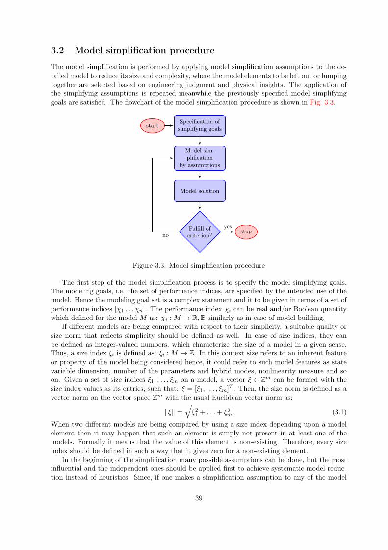
3.2 Model simplification procedure

The model simplification is performed by applying model simplification assumptions to the de-tailed model to reduce its size and complexity, where the model elements to be left out or lumpingtogether are selected based on engineering judgment and physical insights. The application ofthe simplifying assumptions is repeated meanwhile the previously specified model simplifyinggoals are satisfied. The flowchart of the model simplification procedure is shown in Fig. 3.3.

startSpecification ofsimplifying goals

Model sim-plification

by assumptions

Model solution

Fulfill ofcriterion?

stopyes

no

Figure 3.3: Model simplification procedure

The first step of the model simplification process is to specify the model simplifying goals.The modeling goals, i.e. the set of performance indices, are specified by the intended use of themodel. Hence the modeling goal set is a complex statement and it to be given in terms of a set ofperformance indices [χ1 . . . χn]. The performance index χi can be real and/or Boolean quantitywhich defined for the model M as: χi :M → R,B similarly as in case of model building.

If different models are being compared with respect to their simplicity, a suitable quality orsize norm that reflects simplicity should be defined as well. In case of size indices, they canbe defined as integer-valued numbers, which characterize the size of a model in a given sense.Thus, a size index ξi is defined as: ξi :M → Z. In this context size refers to an inherent featureor property of the model being considered hence, it could refer to such model features as statevariable dimension, number of the parameters and hybrid modes, nonlinearity measure and soon. Given a set of size indices ξ1, . . . , ξm on a model, a vector ξ ∈ Z

m can be formed with thesize index values as its entries, such that: ξ = [ξ1, . . . , ξm]T . Then, the size norm is defined as avector norm on the vector space Z

m with the usual Euclidean vector norm as:

‖ξ‖ =√

ξ21 + . . .+ ξ2m. (3.1)

When two different models are being compared by using a size index depending upon a modelelement then it may happen that such an element is simply not present in at least one of themodels. Formally it means that the value of this element is non-existing. Therefore, every sizeindex should be defined in such a way that it gives zero for a non-existing element.

In the beginning of the simplification many possible assumptions can be done, but the mostinfluential and the independent ones should be applied first to achieve systematic model reduc-tion instead of heuristics. Since, if one makes a simplification assumption to any of the model

39

elements then it influence all the other elements on the lower level(s) that are related to it.Hence, leaving out balance volume(s) from the model should be tried firstly and then leaving outthe unimportant balance equations and/or mechanisms and finally variable/parameter lumpingshould be considered.

In the next step the output response of the simplified model is derived by solving the simplifiedset of DAEs and the simplified model performance indices are determined accordingly. The testcases to be used are determined based on the desired use of the model and its operation domaincovering the most important dynamic behavior the system is able to produce.

Finally, in the decision making on one hand the model performance indices and on the otherhand the size indices are compared to the specified ones to decide whether the model fulfillsthe simplifying goals or not. If all the goals are fulfilled the simplifying procedure is terminatedotherwise jumps back to make further investigation on the model behavior to apply furtherassumptions or revise the assumptions that previously done to apply better ones.

3.3 Simplification results

In general, the simplified model should retain the major dynamic characteristics of the systemonly and omit all the details that are weakly represented in the outputs where the major dynamiccharacteristics depend on the intended use of the model.

3.3.1 Simplified nonlinear dynamic hybrid model for simulation purposes(M1)

The following properties, defined by performance (Px) and size (Sx) indices of the simplifiedEPC model (M1) are considered below to achieve the simplifying goals, which are in this casefast dynamic simulation with reduced computational effort to make it possible to integrate theEPC model into a complete driveline or a vehicle model.

M1P1. The model variables and parameters should preserve the physical meaning (χM1P1∈ B).

M1P2. The model should be capable of describing the dynamic behavior of the EPC systemwithin 5% deviation in the whole operation domain with respect to the chamber pressureand the piston position (χM1P2

∈ R, χmaxM1P2

= 0.05). This performance index iscalculated by the Euclidean norm as:

χM1P2=√

χ21,M1P2

+ χ22,M1P2

, (3.2)

where χ1,M1P2is the chamber pressure deviation and χ2,M1P2

is the piston positiondeviation. For computing χi,M1P2

an L2 error has been used to measure the devia-tions of the model response, based on the entries of the model output vectors and themeasurement results on the real system as follows:

χi,M1P2=

√√√√ 1

T

∫ T

0

(

yMeasi (t)− yM1

i (t)

yMeasi

)2

dt, (3.3)

where the suffix i refers to the ith output of the model, Meas and M1 refer to thecorresponding output vector of the measurement and simulation respectively. The overline refers to the integral mean of the particular signal and T is the duration of the testcase.

40

M1S1. The model size and complexity should be significantly reduced (ξM1S1∈ R). The size

index is also calculated by the Euclidean norm as:

ξM1S1=

√√√√

8∑

i=1

wiξ2i,M1S1, (3.4)

where ξi,M1S1are the number of the balance volumes (ξ1), state variables (ξ2), control

inputs (ξ3), disturbance inputs (ξ4), parameters (ξ5), hybrid terms (ξ6), relative degree(ξ7) and finally the relative computational time of the simulated time stretch (ξ8), i.e.the calculation time divided by the simulated time. Moreover, in order to achieve theweighted sum of the individual items numbers wi weights are used. The weights shouldreflect the different impact of the indices on the change of the model complexity.

To achieve the specified goals above via systematic model simplification the first step is tosimplifying the balance volumes then the balance equations and finally the transport mechanismsand constitutive equations. Hence, the following assumptions are done:

M1A1. Remove the power stage / valve subsystem dynamics from the model and apply idealvalves in which the opening and closing processes are instantaneous.

This assumption can be done since the power stage / valve subsystem has much faster dynam-ics than the remained model parts considered for position control of the piston. The dynamics ofthe power stage / valve subsystem is considered for the mass flow rate control (see details laterin Section 5.4). This assumption removes the ixx, vxx and xxx terms from the state vector, theUsup term from the disturbance inputs besides, avoid all the parameters related to the powerstage / valve subsystem except αxx and Axx.

M1A2. The thermodynamic processes in the chamber can be considered as isothermal insteadof polytropic.

This assumption can be done, as well, since the focused dynamical range of the modeledprocesses should cover the medium dynamic responses only while the air temperature convergesto the environment temperature with slow dynamics. In this way the temperature in the chambercan be considered with constant value. Thus, the isothermal model class can cover the requiredbehavior. One has to mention that this assumption eliminates the mch state since the chamberbalance equation is derived from the gas mass balance only and the gas energy balance equationis not needed anymore. Moreover, eliminates the Tsup disturbance input by using Tamb.

M1A3. The piston cannot reach its limitations during normal operation.

One of the extreme piston positions, corresponding of the completely exhausted chamber, isdetermined by the stiffness of the disc and helper springs without reaching the stroke limitation(xlim,1

pst ). Besides, the piston stroke is large enough to cover the working domain of the clutch

mechanism without reaching the other stroke limitation (xlim,2pst ). This assumption results that

the piston limiting term (F limpst ) can be left out of the model, which reduces the number of the

hybrid modes and eliminates the computational effort regarding the collisions with the strokelimiters.

M1A4. Subsonic flow in both of the intake and exhaust direction cannot be reached simultane-ously.

41

The necessary conditions for achieving subsonic flow in both of the two directions are fulfilled,when Πl > Πcrit and Πe > Πcrit, is pamb/psup > Π2

crit. But this condition has not been satisfiedsince it is out of the (disturbance) input constraints of the EPC (see the input constraints inSection 2.3).

M1A5. The friction force term (Ffr) can be approximated using sigmoid function as follows:

Ffr = µpst (pch − pamb)Apst

(2

1− e−ufrvpst− 1

)

, (3.5)

where ufr determines the friction force steepness at small velocities. This helps to solve thenumerical problems for eliminating the hybrid modes regarding the friction force.

M1A6. The cross sections and the contraction coefficients can be lumped together.

The new, i.e. effective, cross section terms are obtained as follows: Aeffxx = αxxAxx.

M1A7. For the sake of simplicity, the spring term shsp(xpst,0 − xpst) can be integrated into theFl(xpst) term.

Applying these assumptions above the state space description of the simplified model forsimulation purposes is obtained. From the simplified DAEs of the model the state vector iscomposed as follows:

xM1= [ pch vpst xpst ]T . (3.6)

The control input vector (uM1), that includes the duty cycle of the PWM control signals of

the SMVs, is not changed (see Eq. (2.48)), while the disturbance input vector includes only thecompressed air pressure, ambient- pressure and temperature respectively:

dM1=[psup pamb Tamb

]T. (3.7)

The output vector includes the chamber pressure, the piston position and the supply pressure:

yM1=[pch xpst psup

]T. (3.8)

The simplified state space model has the form of Eq. (2.50), as well, where the nonlinearstate functions are written as follows (the entries that depend on the hybrid modes are boxed,too):

f(k)1,M1

=R

(

md,sl Aeffsl +md,bl A

effbl

)

ξl Tamb

V dch + xpstApst

−

−R

(

md,se Aeffse +md,be A

effbe

)

ξe Tamb

V dch + xpstApst

−

−pch vpstApst

V dch + xpstApst

,

(3.9)

f(k)2,M1

=(pch − pamb)Apst − vpstkpst − Fl(xpst)

mpst−

−µpst(pch − pamb)Apst

(2

1−e−ufrvpst

− 1)

mpst,

(3.10)

f(k)3,M1

= vpst, (3.11)

42

where

ξl =

√

2 κ

κ− 1

p2supRTamb

(

Πl

2κ − Πl

κ+1κ

)

and (3.12)

ξe =

√

2 κ

κ− 1

p2chRTamb

(

Πe

2κ − Πe

κ+1κ

)

. (3.13)

The output equation has the form of Eq. (2.69), as well, where

CM1=

1 0 00 0 10 0 0

(3.14)

and the EM1matrix corresponds to the measured disturbance which is the psup, hence it is

written as follows:

EM1=

0 0 00 0 01 0 0

. (3.15)

The performance output is generated from the measured output by the following simpleequation:

zM1= [ 0 1 0 ]yM1

. (3.16)

The simulation result of the simplified model (M1) is shown in Fig. 3.4.

0

0.5

1

1.5

2

2.5

3

3.5

4

4.5x 10

5

pch

[Pa]

Measurement M0 M1 M2

0 0.2 0.4 0.6 0.8 1 1.20

2

4

6

8

10

12

14

xpst

[mm

]

time [s]

Figure 3.4: EPC measurement and simulation results in case of model M0, M1 and M2

43

Besides, the measurement on the real system and the response of the detailed model (M0)for the same inputs are shown, as well. The input signals are derived from a real clutching.The disengagement has been executed with maximal dynamics to reach the disengagement stateas quickly as possible. Then, the engagement has been started with fast dynamics as well toreach the touch point, where the pressure plate and the friction disc have been connected. Inthe clutching domain the stroke has been decreased slowly to increase the transmitted torquesmoothly. Finally, in the end of the engagement the engagement state has been set up withmaximal dynamics as well.

The most important results of this simplifying procedure are as follows. All the retainedsystem variables have preserved their physical meaning meanwhile, some model parameters (αxx

and Axx) have changed slightly their meaning (Aeffxx = αxxAxx) due to the lumping (χM1P1

=true). The pressure deviation of M1 comparing with M0 has been increased from 1.23% to2.38%, the position deviation has been increased from 2.63% to 3.43% and the total deviationhas been increased from 2.9% to 4.18% hence, the required accuracy has been fulfilled (χM1P2

<χmaxM1P2

).The number of the balance volumes for which the balance equations are applied has been

reduced from 10 to 2. The hierarchy structure of the simplified model is shown in Fig. 3.5where, the term which has hybrid behavior is depicted by dashed line. The number of the

balance volume level

balance equation level

transport mechanismand constitutive level

Simplified nonlinear dynamic modelfor simulation purposes

Pistonbalance volume

Chamberbalance volume

Momentumbalance

vpst, xpst

Massbalance

pch

Pressureterm

Apst, pamb

Dampingterm

kpst

Loadterm

Fload(xpst)

Frictionterm

µpst, Apst,

pamb, ufr

Convectiveterm

κ, R,

Aeffxx, V

dch,

Apst, psup,

Tamb, pamb

Figure 3.5: Hierarchical structure of the simplified nonlinear dynamic hybrid model for simulationpurposes

state variables has been reduced from 16 to 3, the control inputs have been unchanged underthis simplification process and the disturbance variables has been cut to 3 from the original 5.The variable structure graph of the simplified model is shown in Fig. 3.6. The number of theparameters has been reduced from 83 to 12 where the Fl (xpst) term, i.e. the center characteristicline of the clutch mechanism, has been considered as a third order polynomial [39]. The equationshave been simplified considerably by eliminating the power stage / valve subsystem and the gas

44

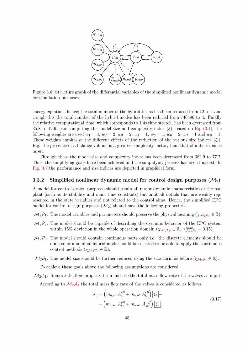
md,sl

md,bl

md,se

md,be

pch vpst xpst

psuppambTamb

Figure 3.6: Structure graph of the differential variables of the simplified nonlinear dynamic modelfor simulation purposes

energy equations hence; the total number of the hybrid terms has been reduced from 12 to 1 andtrough this the total number of the hybrid modes has been reduced from 746496 to 4. Finallythe relative computational time, which corresponds to 1.4s time stretch, has been decreased from35.8 to 12.6. For computing the model size and complexity index (ξ), based on Eq. (3.4), thefollowing weights are used w1 = 4, w2 = 2, w3 = 2, w4 = 1, w5 = 1, w6 = 2, w7 = 1 and w8 = 1.These weights emphasize the different effects of the reduction of the various size indices (ξi).E.g. the presence of a balance volume is a greater complexity factor, than that of a disturbanceinput.

Through these the model size and complexity index has been decreased from 382.9 to 77.7.Thus, the simplifying goals have been achieved and the simplifying process has been finished. InFig. 3.7 the performance and size indices are depicted in graphical form.

3.3.2 Simplified nonlinear dynamic model for control design purposes (M2)

A model for control design purposes should retain all major dynamic characteristics of the realplant (such as its stability and main time constants) but omit all details that are weakly rep-resented in the state variables and not related to the control aims. Hence, the simplified EPCmodel for control design purposes (M2) should have the following properties:

M2P1. The model variables and parameters should preserve the physical meaning (χM2P1∈ B).

M2P2. The model should be capable of describing the dynamic behavior of the EPC systemwithin 15% deviation in the whole operation domain (χM2P2

∈ R, χmaxM2P2

= 0.15).

M2P3. The model should contain continuous parts only i.e. the discrete elements should beomitted or a nominal hybrid mode should be selected to be able to apply the continuouscontrol methods (χM2P3

∈ B).

M2S1. The model size should be further reduced using the size norm as before (ξM2S1∈ R).

To achieve these goals above the following assumptions are considered:

M2A1. Remove the flow property term and use the total mass flow rate of the valves as input.

According to M2A1 the total mass flow rate of the valves is considered as follows:

σv =(

md,sl Aeffsl +md,bl A

effbl

)

ξl −

−(

md,se Aeffse +md,be A

effbe

)

ξe .(3.17)

45

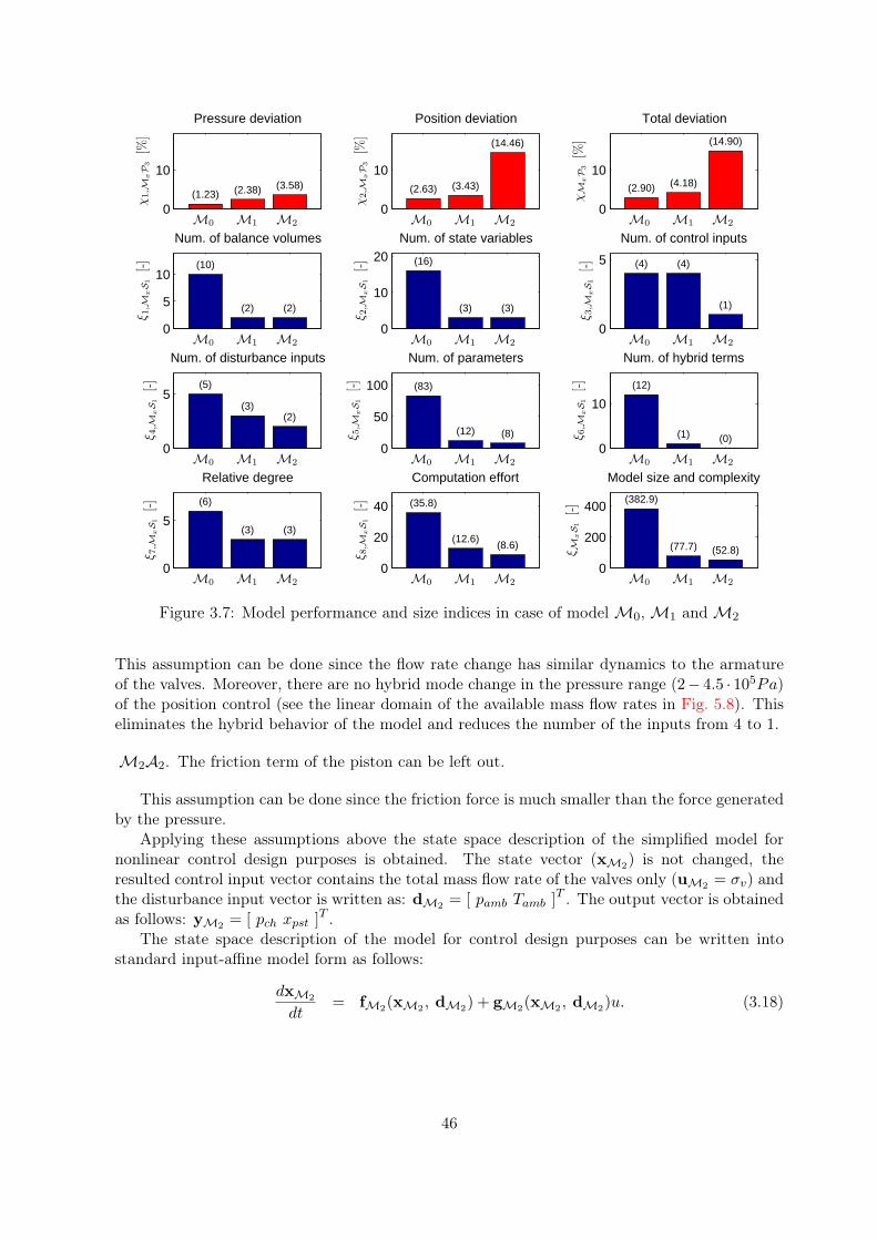
0

10

χ1,M

xP

3[%

]

M0 M1 M2

Pressure deviation

(1.23) (2.38) (3.58)

0

10

χ2,M

xP

3[%

]

M0 M1 M2

Position deviation

(2.63) (3.43)

(14.46)

0

10

χM

xP

3[%

]

M0 M1 M2

Total deviation

(2.90) (4.18)

(14.90)

0

5

10

ξ 1,M

xS1

[-]

M0 M1 M2

Num. of balance volumes

(10)

(2) (2)

0

10

20

ξ 2,M

xS1

[-]

M0 M1 M2

Num. of state variables

(16)

(3) (3)

0

5

ξ 3,M

xS1

[-]

M0 M1 M2

Num. of control inputs

(4) (4)

(1)

0

5

ξ 4,M

xS1

[-]

M0 M1 M2

Num. of disturbance inputs

(5)

(3)(2)

0

50

100

ξ 5,M

xS1

[-]

M0 M1 M2

Num. of parameters

(83)

(12) (8)

0

10

ξ 6,M

xS1

[-]

M0 M1 M2

Num. of hybrid terms

(12)

(1) (0)

0

5

ξ 7,M

xS1

[-]

M0 M1 M2

Relative degree

(6)

(3) (3)

0

20

40

ξ 8,M

xS1

[-]

M0 M1 M2

Computation effort

(35.8)

(12.6)(8.6)

0

200

400

ξ MxS1

[-]

M0 M1 M2

Model size and complexity

(382.9)

(77.7) (52.8)

Figure 3.7: Model performance and size indices in case of model M0, M1 and M2

This assumption can be done since the flow rate change has similar dynamics to the armatureof the valves. Moreover, there are no hybrid mode change in the pressure range (2− 4.5 · 105Pa)of the position control (see the linear domain of the available mass flow rates in Fig. 5.8). Thiseliminates the hybrid behavior of the model and reduces the number of the inputs from 4 to 1.

M2A2. The friction term of the piston can be left out.

This assumption can be done since the friction force is much smaller than the force generatedby the pressure.

Applying these assumptions above the state space description of the simplified model fornonlinear control design purposes is obtained. The state vector (xM2

) is not changed, theresulted control input vector contains the total mass flow rate of the valves only (uM2

= σv) andthe disturbance input vector is written as: dM2

= [ pamb Tamb ]T . The output vector is obtained

as follows: yM2= [ pch xpst ]

T .The state space description of the model for control design purposes can be written into

standard input-affine model form as follows:

dxM2

dt= fM2

(xM2, dM2

) + gM2(xM2

, dM2)u. (3.18)

46

The coordinate functions are written as follows:

f1,M2= −

pch vpstApst

V dch + xpstApst

, (3.19)

f2,M2=

(pch − pamb)Apst − vpstkpst − Fl(xpst)

mpst, (3.20)

f3,M2= vpst, (3.21)

g1,M2=

RTamb

V dch + xpstApst

, (3.22)

g2,M2= 0, (3.23)

g3,M2= 0. (3.24)

The measured output is written as the following linear equation:

yM2= CM2

xM2, (3.25)

where

CM2=

[1 0 00 0 1

]

. (3.26)

The performance output is generated from the measured output by the following simpleequation:

zM2= [ 0 1 ]yM2

. (3.27)

The simulation results of this simplified model (M2) are shown in Fig. 3.4, as well. It can beseen that the outputs of M2 have a deviation, which is mainly caused by the neglected friction.

The most important results of this simplifying procedure are as follows. All the retained modelvariables and parameters have preserved their physical meaning (χM2P1

= true). Since all thediscrete switching terms have been eliminated the model became continuous (χ M2P3

= true).The pressure deviation of M2 comparing with M1 has been increased from 2.38% to 3.58%,the position deviation has been increased from 3.43% to 14.46% and the total deviation hasbeen increased from 4.18% to 14.9% (see Fig. 3.7) nevertheless, the required accuracy has beenfulfilled (χM2P2

< χmaxM2P2

).The number of the balance volumes has been invariant under this simplification process (see

Fig. 3.7). The hierarchy structure of M2 is shown in Fig. 3.8. The number of the state variableshas been invariant as well while the control inputs have been reduced from 4 to 1, the disturbancevariables have been reduced from 3 to 2 and the number of the parameters has been reducedfrom 12 to 8. The variable structure graph of M2 is shown in Fig. 3.9. Finally the relativecomputational time, which corresponds to 1.4s time stretch has also been decreased further from12.6 to 8.6. Through these the M2 size and complexity index, using the same weights as before,has been decreased from 77.7 to 52.8. Thus, the simplifying goals have been achieved and thesimplifying process has been finished.

3.4 Summary

A systematic approach is applied in this chapter for model simplification using engineering judg-ment and physical insight to find model elements to be left out or simplified. The model sim-plification is performed by applying simplifying assumptions to the model, which are done in asystematic way using the hierarchy tree of the model. Moreover, performance and size indicesare used to decide whether the simplified models fulfill the predefined simplifying goals or not.

47

balance volume level

balance equation level

transport mechanismand constitutive level

Simplified nonlinear dynamic modelfor control purposes

Pistonbalance volume

Chamberbalance volume

Momentumbalance

vpst, xpst

Massbalance

pch

Pressureterm

Apst, pamb

Loadterm

Fload(xpst)

Dampingterm

kpst

Convectiveterm

σv, R,

V dch, Apst,

Tamb, pamb

Figure 3.8: Hierarchical structure of the simplified nonlinear dynamic model for control purposes

σv pch vpst xpst

pambTamb

Figure 3.9: Structure graph of the differential variables of the simplified model for control pur-poses

The approach is applied for simplifying the dynamic hybrid model of the EPC system thatwas originally developed from first engineering principles. Using this approach two simplifiedmodels are derived. One of them for fast dynamic simulation with reduced computational effortto make it possible to integrate the model into a complete driveline or a vehicle model. Theother for control design purposes in which all major dynamic characteristics of the real systemare retained and all details that are weakly represented in the state variables and not related tothe control aims are omitted.

As one might expect, the complexity of the models are decreased significantly e.g., the numberof the states reduced from 16 to 3. The output errors of the resulted models are increasedwith the model simplification, nevertheless they remained in the acceptable range. Hence thesimplification aims are satisfied with the resulted simplified models. Besides, the model classis changed from discrete-continuous to pure continuous in case of the control oriented model.Hence, the state equations of this model can be written into the standard input affine formwhich is suitable for control design purposes.

48

Chapter 4

Model analysis

A model based controller design usually requires information about the dynamic properties ofthe model that influences the applicable control significantly. This information is supplied by themodel analysis. In most cases the nonlinear model analysis is based on determining the followingthree basic dynamic properties of the model: controllability, observability and stability. If thereare additional preferences or requirements that determine the possible controller types, thisanalysis can be restricted or extended with other investigations.

A comprehensive description of the available methods regarding nonlinear system analysiscan be found in the following books [40, 41, 42, 43], while the linear system analysis is discussedin [44, 45]. A process control focused analysis of linear and nonlinear systems is presented in[46].

In this case the aim of the model analysis is to perform an exhaustive investigation to dealwith the key properties of the control oriented model and to cover the required dynamic propertiesrelevant to controller design.

The control oriented model is in standard nonlinear input-affine state-space form as:

dx

dt= f(x) +

m∑

i=1

gi(x)ui, (4.1)

where m is the number of the control inputs (see Eq. (3.18)-(3.24)).The output equations are written as follows:

yj = hj(x), j = 1, . . . , r, (4.2)

where r is the number of the outputs.From Eq. (3.25)-(3.27) the output function for the control oriented model is obtained as:

h(x) = xpst. (4.3)

The main topics of the model analysis covered in this chapter consists of the following items:

• Checking the basic properties of the control oriented model such as the controllability,observability and stability.

• Analysis relative degree and zero dynamics of the model to examine the internal behaviorof the system.

• Analysis of the model sensitivity with respect to parametric uncertainty and disturbancesignals.

49

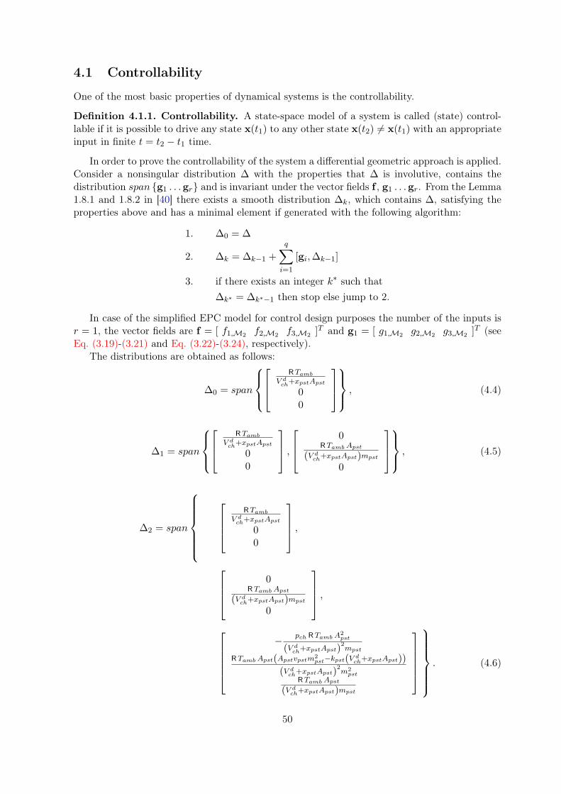
4.1 Controllability

One of the most basic properties of dynamical systems is the controllability.

Definition 4.1.1. Controllability. A state-space model of a system is called (state) control-lable if it is possible to drive any state x(t1) to any other state x(t2) 6= x(t1) with an appropriateinput in finite t = t2 − t1 time.

In order to prove the controllability of the system a differential geometric approach is applied.Consider a nonsingular distribution ∆ with the properties that ∆ is involutive, contains thedistribution span g1 . . .gr and is invariant under the vector fields f , g1 . . .gr. From the Lemma1.8.1 and 1.8.2 in [40] there exists a smooth distribution ∆k, which contains ∆, satisfying theproperties above and has a minimal element if generated with the following algorithm:

1. ∆0 = ∆

2. ∆k = ∆k−1 +

q∑

i=1

[gi,∆k−1]

3. if there exists an integer k∗ such that

∆k∗ = ∆k∗−1 then stop else jump to 2.

In case of the simplified EPC model for control design purposes the number of the inputs isr = 1, the vector fields are f = [ f1,M2

f2,M2f3,M2

]T and g1 = [ g1,M2g2,M2

g3,M2]T (see

Eq. (3.19)-(3.21) and Eq. (3.22)-(3.24), respectively).The distributions are obtained as follows:

∆0 = span

RTamb

V dch

+xpstApst

00

, (4.4)

∆1 = span

RTamb

V dch

+xpstApst

00

,

0RTamb Apst

(V dch

+xpstApst)mpst

0

, (4.5)

∆2 = span

RTamb

V dch

+xpstApst

00

,

0RTamb Apst

(V dch

+xpstApst)mpst

0

,

−pch RTamb A

2pst

(V dch

+xpstApst)2mpst

RTamb Apst(Apstvpstm2pst−kpst(V d

ch+xpstApst))(V d

ch+xpstApst)

2m2

pstRTamb Apst

(V dch

+xpstApst)mpst

. (4.6)

50

The ∆2 distribution spans the whole R3, since its elements are non-zero functions that are

linearly independent in any point of the state-space. This means that the system is controllableby the mass flow rate of the valves (σv) at any point of the state space.

4.2 Observability

The next basic properties of dynamical systems is the observability.

Definition 4.2.1. Observability. Given the inputs and the outputs of a system over a finitetime interval. If it is possible to determine the value of the states based on these values anda state-space system model in such a way that the functions of inputs and outputs and theirderivatives are used, then the system is called (state) observable.

In order to prove the observability of the system a differential geometric approach is appliedas well. Consider a nonsingular distribution ∆ again with the properties that ∆ is involutive,contained in the distribution (span dh(x)1 . . . dh(x)m)⊥ and is invariant under the vector fieldsf , g1 . . .gr, where dh(x)j is defined as the 1 × n row vector whose i-th element is the partialderivative of h(x)j with respect to xi. Since the existence of a nonsingilar distribution ∆ whichsatisfies the properties above implies and is implied by the existence of a codistribution Ω (namely∆⊥) with the properties that Ω is spanned by exact covectorfields, contains the codistributionspan dh(x)1 . . . dh(x)m and is invariant under the vector fields f , g1 . . .gr. From the Lemma1.9.1 and 1.9.2 in [40] there exists a smooth codistribution Ωk, which contains Ω, satisfying theproperties above and has a minimal element if generated with the following algorithm:

1. Ω0 = span dh(x)1 . . . dh(x)m

2. Ωk = Ωk−1 +

q∑

i=1

LfiΩk−1

3. if there exists an integer k∗ such that

Ωk∗ = Ωk∗−1 then stop else jump to 2.

For the EPC the codistributions are obtained as follows:

Ω0 = span[

0 0 1], (4.7)

Ω1 = span[

0 0 1],[0 1 0

], (4.8)

Ω2 = span[

0 0 1],[0 1 0

],[

Apst

mpst−

kpstmpst

−dFl(xpst)/dxpst

mpst

]

. (4.9)

The Ω2 codistribution spans the whole R3, since its elements are non-zero functions that are

linearly independent in any point of the state-space. This means that the system is observableby the performance output (xpst) at any point of the state-space.

Minimal models are known to be jointly reachable and detectable [40, 16]. Since the modelhas these properties, the model is minimal.

4.3 Stability

The third basic property of dynamical systems is stability. The most complete contribution tothe stability analysis of nonlinear dynamical systems is due to Lyapunov [47].

Lyapunov’s indirect or linearization method is concerned with the local stability of nonlinearsystems. It is a formalization of the intuition that a nonlinear system should behave similarly to

51

its linearized approximation for small ranges. Moreover, the global asymptotic stability propertyis implied by the local asymptotic stability in all the operation points as follows [43]:

• If the linearized system is strictly stable i.e, if all eigenvalues of A are strictly in the left-half complex plane, then the equilibrium point is asymptotically stable for the actualnonlinear system.

• If the linearized system is unstable i.e, if at least one eigenvalue of A is strictly inthe right-half complex plane, then the equilibrium point is unstable for the nonlinearsystem.

• If the linearized system is marginally stable i.e, all eigenvalues of A are in the left-half complex plane, but at least one of them is on the imaginary axis, then one cannotconclude anything from the linear approximation. The equilibrium point may be stable,asymptotically stable, or unstable for the nonlinear system.

Lyapunov’s direct method, along with the Barbashin-Krasovskii-LaSalle invariance principle[48, 49, 50], provide more powerful framework for analyzing the stability of nonlinear dynamicalsystems. In particular, Lyapunov’s direct method can provide local and global stability con-clusions of an equilibrium point of a nonlinear dynamical system if a smooth positive-definitefunction of the nonlinear system states (Lyapunov function) can be constructed for which itstime rate of change due to perturbations in a neighborhood of the system’s equilibrium is alwaysnegative or zero, with strict negative definiteness ensuring asymptotic stability. Alternatively,using the Barbashin-Krasovskii-LaSalle invariance principle the positive-definite condition onthe Lyapunov function as well as the strict negative- definiteness condition on the Lyapunovderivative can be relaxed while assuring asymptotic stability. In particular, if a smooth functiondefined on a compact invariant set with respect to the nonlinear dynamical system can be con-structed whose derivative along the system’s trajectories is negative semi-definite and no systemtrajectories can stay indefinitely at points where the function’s derivative identically vanishes,then the system’s equilibrium is asymptotically stable [51].

The definitions and theorems in terms of stability are given below [41, 43, 40, 46].The stability analysis is concerned with general differential equation in the form

x = f(x, t), x (x0) = x0, (4.10)

where x ∈ Rn and t ≥ 0. The system defined by Eq. (4.10) is said to be autonomous. Moreover,

it is assumed that f(x, t) is piecewise continuous with respect to t.

Definition 4.3.1. Equilibrium point. x∗ is said to be an equilibrium point of Eq. (4.10) iff(x∗, t) ≡ 0 for all t > 0.

It should be noted that x0 can be made an equilibrium point of Eq. (4.10) by translating theorigin to the equilibrium point x∗.

Definition 4.3.2. Stability in the sense of Lyapunov. The equilibrium point f(x∗, t) = 0

is called a stable equilibrium point of Eq. (4.10) if for all t0 ≥ 0 and ǫ > 0, there exist δ (t0, ǫ)such that

|x0| < δ (t0, ǫ) ⇒ |x(t)| < ǫ ∀t ≥ t0, (4.11)

where x(t) is the solution of Eq. (4.10) starting for x0 at t0.

Definition 4.3.3. Uniform stability. The equilibrium point f(x∗, t) = 0 is called a uniformlystable equilibrium point of Eq. (4.10) if in the preceding definition δ can be chosen independentof t0.

52

Definition 4.3.4. Asymptotic stability. The equilibrium point f(x∗, t) = 0 is an asymptoti-cally stable equilibrium point of Eq. (4.10) if

• f(x∗, t) = 0 is a stable equilibrium point of Eq. (4.10),

• f(x∗, t) = 0 is attractive, that is for all t0 ≥ 0 there exists a δ (t0) such that

|x0| < δ (t0, ǫ) ⇒ limt→∞

|x(t)| = 0. (4.12)

Definition 4.3.5. Uniform asymptotic stability. The equilibrium point f(x∗, t) = 0 is anuniformly asymptotically stable equilibrium point of Eq. (4.10) if

• f(x∗, t) = 0 is a uniformly stable equilibrium point of Eq. (4.10),

• The trajectory x(t) converges uniformly to 0, that is, there exists δ > 0 and a functionγ(τ,x0) : R+×R

n 7→ R+ such that limτ→∞

γ(τ,x0) = 0 for all x0 ∈ Bδ, where Bδ is a ball

of radius δ centered at the origin, and

|x0| < δ ⇒ |x(t)| ≤ γ(t− t0,x0) ∀t ≥ t0. (4.13)

The previous definitions are local, since they concern neighborhoods of the equilibrium point.Global asymptotic stability and global uniform asymptotic stability are defined as follows:

Definition 4.3.6. Global asymptotic stability. The equilibrium point f(x∗, t) = 0 is aglobally asymptotically stable equilibrium point of Eq. (4.10) if it is asymptotically stable andlimt→∞

x(t) = 0 for all x0 ∈ Rn.

Definition 4.3.7. Global uniform asymptotic stability. The equilibrium point f(x∗, t) = 0

is a globally, uniformly, asymptotically stable equilibrium point of Eq. (4.10) if it is globallyasymptotically stable and if in addition, the convergence to the origin of trajectories is uniformin time, that is to say that there is a function γ(τ,x0) : R+ × R

n 7→ R+ such that

|x(t)| ≤ γ(t− t0,x0) ∀t ≥ t0. (4.14)

Definition 4.3.8. Positive definite function. A scalar continuous function V (x) is said tobe locally positive definite if V (0) = 0 and, in a ball Bδ x 6= 0 ⇒ V (x) > 0. If V (0) = 0 andthe above property holds over the whole state space, then V (x) is said to be globally positivedefinite.

A few related concepts can be defined similarly, in a local or global sense, i.e., a functionV (x) is negative definite if −V (x) is positive definite; V (x) is positive semi-definite if V (0) = 0

and V (x) ≥ 0 for x 6= 0; V (x) is negative semi-definite if −V (x) is positive semi-definite. Theprefix ”semi” is used to reflect the possibility of V being equal to zero for (x) 6= 0.

Definition 4.3.9. Lyapunov function. If, in a ball Bδ, the function V (x) is positive definiteand has continuous partial derivatives, and if its time derivative along any state trajectory ofsystem Eq. (4.10) is negative semi-definite, i.e., V (x) ≤ 0 then V (x) is said to be a Lyapunovfunction for the system Eq. (4.10).

The relations between Lyapunov functions and the stability of systems are made precisein a number of theorems in Lyapunov’s direct method. Such theorems usually have local andglobal versions. The local versions are concerned with stability properties in the neighborhoodof equilibrium point and usually involve a locally positive definite function.

53

Theorem 4.3.1. Local stability. If, in a ball Bδ, there exists a scalar function V (x) withcontinuous first partial derivatives such that

• V (x) is positive definite (locally in Bδ)

• V (x) is negative semi-definite (locally in Bδ)

then the equilibrium point 0 is stable. If, actually, the derivative V (x) is locally negative definitein Bδ, then the stability is asymptotic.

The above theorem applies to the local analysis of stability. In order to assert global asymp-totic stability of a system, one might naturally expect that the ball Bδ in the above local theoremhas to be expanded to be the whole state-space. This is indeed necessary, but it is not enough. Anadditional condition on the function V (x) has to be satisfied: V (x) must be radially unbounded,i.e. V (x) → ∞ as |x| → ∞.

Theorem 4.3.2. Global stability. Assume that there exists a scalar function V (x) with con-tinuous first partial derivatives such that

• V (x) is positive definite

• V (x) is negative semi-definite

• V (x) → ∞ as |x| → ∞

then the equilibrium at the origin is globally stable. If, actually, the derivative V (x) is negativedefinite, then the stability is globally asymptotic.

Asymptotic stability of a system is usually a very important property to be determined.However, the theorems just described are often difficult to apply in order to assert this property.The reason is that it often happens that V (x), the derivative of the Lyapunov function candidate,is only negative semi-definite. In this kind of situation, it is still possible to draw conclusions onasymptotic stability, with the help of the powerful invariant set theorems, attributed to La’Salle.The central concept in these theorems is that of invariant set, a generalization of the concept ofequilibrium point.

Definition 4.3.10. Invariant set. A set G is an invariant set for a dynamic system if everysystem trajectory which starts from a point in G remains in G for all future time.

For instance, any equilibrium point is an invariant set. The domain of attraction of anequilibrium point is also an invariant set. A trivial invariant set is the whole state-space. For anautonomous system, any of the trajectories in state-space is an invariant set.

The invariant set theorems make it possible to extend the concept of Lyapunov function soas to describe convergence to dynamic behaviors when V (x), the derivative of the Lyapunovfunction candidate, is only negative semi-definite.

Theorem 4.3.3. Local invariant set theorem. Consider an autonomous system of the formEq. (4.10), with f(x) continuous, and let V (x) be a scalar function with continuous first partialderivatives. Assume that

• for some l > 0, the region Ωl defined by V (x) < l is bounded

• V (x) ≤ 0 for all x in Ωl

Let R be the set of all points within Ωl where V (x) = 0, and M be the largest invariant set inR. Then, every solution x(t) originating in Ωl tends to M as t→ ∞.

54

Corollary 4.3.1. Consider the autonomous system Eq. (4.10), with f(x) continuous, and letV (x) be a scalar function with continuous partial derivatives. Assume that in a certain neigh-borhood Ω of the origin

• V (x) is locally positive definite

• V (x) is negative semi-definite

• the set R defined by V (x) = 0 contains no trajectories of Eq. (4.10) other than thetrivial trajectory x ≡ 0

then, the equilibrium point 0 is asymptotically stable. Furthermore, the largest connected regionof the form Ωl (defined by V (x) < l) within Ω is a domain of attraction of the equilibrium point.

Indeed, the largest invariant set M in R then contains only the equilibrium point 0.The above invariant set theorem and its corollary can be simply extended to a global result,

by requiring the radial unboundedness of the scalar function V (x) rather than the existence ofa bounded Ωl.

Theorem 4.3.4. Global invariant set theorem. Consider an autonomous system of the formEq. (4.10), with f(x) continuous, and let V (x) be a scalar function with continuous first partialderivatives. Assume that

• V (x) is positive definite

• V (x) → ∞ as |x| → ∞

• V (x) ≤ 0 over the whole state-space

Let R be the set of all points where V (x) = 0, and M be the largest invariant set in R. Then,all solutions globally asymptotically converge to M as t→ ∞.

4.3.1 Stability analysis applying Lyapunov’s indirect method

A linear time-invariant (LTI) system (see the state space realization in Eq. (B.1)) is internallystable if and only if all the eigenvalues of the state matrix A have strictly negative real parts:

Re λi (A) < 0, ∀i. (4.15)

For this purpose the control oriented model has been linearized around a typical equilibriumstate. The linearization can be seen in Section B.1 of Appendix B.

In order to prove that all the eigenvalues of A have strictly negative real parts the Routh-Hurwitz stability criterion is used [52]. This method helps to determine whether all the roots ofthe characteristic polynomial of the linear system P (λ) = det (λI−A), i.e. the eigenvalues ofA, have negative real parts.

The general realization of the Routh-Hurwitz stability criterion is as follows [53]:

∆1 > 0, ∆2 > 0, . . . , ∆n > 0, (4.16)

where

∆k = det

a1 1 0 0 0 0 · · · 0a3 a2 a1 1 0 0 · · · 0a5 a4 a3 a2 a1 0 · · · 0...

......

......

.... . .

...a2k−1 a2k−2 a2k−3 a2k−4 a2k−5 a2k−6 · · · ak

. (4.17)

55

In case of the linearized model of the EPC system the characteristic polynomial is written asfollows:

P (λ) = λ3 + a1λ2 + a2λ+ a3, (4.18)

where

a1 =kpstmpst

, (4.19)

a2 =

ddxpst

Fl(x∗pst)

mpst+

p∗chA2pst

(V dch +Apstx∗pst

)mpst

and (4.20)

a3 = 0. (4.21)

From Eq. (4.16) and Eq. (4.17) the Routh-Hurwitz stability criterion for third order systemsis obtained as:

a1 > 0, (4.22)

a1a2 − a3 > 0 and (4.23)

(a1a2 − a3)a3 > 0. (4.24)

Since the kpst and mpst parameters for physical systems is always greater than zero, the firststability criterion defined by Eq. (4.22) for the EPC system is inherently satisfied.

The second criterion defined by Eq. (4.23) is written as follows:

d

dxpstFl(x

∗pst) +

p∗chA2pst

V dch +Apstx∗pst

> 0. (4.25)

The third criterion is obviously not satisfied since, from Eq. (4.18) and Eq. (4.21) one polemust be equal to zero. Hence, the analysis shows that the linearized model has a pole equal tozero and has two stable or unstable poles depending on its parameters and the equilibrium pointused for the linearization. Thus the linearized model can be marginally stable or unstable.

In case of a given EPC system the area of the piston (Apst) is fixed, but the dead volumeof the chamber (V d

ch) and the stiffness of the clutch spring (dFl(xpst)/dxpst) can vary duringthe lifetime of the system, hence these parameter changes should be considered in the design ofthe system. In Fig. 4.1 different equilibrium points are shown over the pressure-position planewith increasing dead volume on the third axis to demonstrate the parameter dependance of thestability. The unstable and marginally stable equilibrium points are depicted with red and blackpoints, respectively.

Consequently, the nonlinear system have locally unstable equilibrium points depending on itsparameters and have equilibrium points, which may be stable, asymptotically stable, or unstable.In order to conclude the stability of the EPC system further investigations are needed applyingLyapunov’s direct method.

4.3.2 Stability analysis applying Lyapunov’s direct method

The basic philosophy of Lyapunov’s direct method is the mathematical extension of a funda-mental physical observation: if the total energy of a system is continuously dissipated, then thesystem, whether linear or nonlinear, must eventually settle down to an equilibrium point. Thus,it may conclude the stability of a system by examining the variation of a single scalar function.

The Lyapunov function candidate is the total energy of the EPC system, namely,

V (x,d) =

∫

mpstvpstdxpst +

∫

(pch − pamb)dVch +

∫

Fl(xpst)dxpst. (4.26)

56

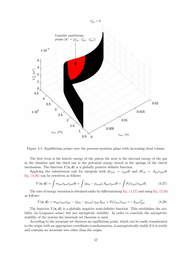
0

0.005

0.01

0.015

0.02

0.5

1

1.5

2

2.5

3

3.5

4

4.5

x 105

0

1

2

3

4

x 10−3

Vd ch

[m3]

v∗pst = 0

xpst [m]pch [Pa]

Unstable equilibriumpoints (x∗ = [p∗

ch , v∗pst , x

∗pst ])

Figure 4.1: Equilibrium points over the pressure-position plane with increasing dead volume

The first term is the kinetic energy of the piston the next is the internal energy of the gasin the chamber and the third one is the potential energy stored in the springs of the clutchmechanism. The function V (x,d) is a globally positive definite function.

Applying the substitution rule for integrals with dxpst = vpstdt and dVch = ApstvpstdtEq. (4.26) can be rewritten as follows:

V (x,d) =

∫

mpstvpstvpstdt+

∫

(pch − pamb)Apstvpstdt+

∫

Fl(xpst)vpstdt. (4.27)

The rate of energy variation is obtained easily by differentiating Eq. (4.27) and using Eq. (3.20)as follows:

V (x,d) = mpstvpstvpst − (pch − pamb) vpstApst + Fl(xpst)vpst = −kpstv2pst. (4.28)

The function V (x,d) is a globally negative semi-definite function. This establishes the sta-bility (in Lyapunov sense) but not asymptotic stability. In order to conclude the asymptoticstability of the system the invariant set theorem is used.

According to the invariant set theorem an equilibrium point, which can be easily transformedto the origin with an appropriate coordinate transformation, is asymptotically stable if it is stableand contains no invariant sets other than the origin.

57

If Eq. (4.25) is satisfied for the EPC system over the whole state-space then there are nounstable equilibrium points. Only a single equilibrium point exists along a trajectory, which isglobally asymptotically stable according to the invariant set theorem.

Since the convergence to the origin of trajectories of the EPC is uniform in time, i.e. thetrajectories are independent of t0, the system has the uniform property, too.

Thus the EPC system is globally uniformly asymptotically stable if the Eq. (4.25) is satisfiedotherwise, the equilibrium points where Eq. (4.25) is not satisfied are unstable and the remainedones are locally uniformly asymptotically stable.

4.4 Zero dynamics

The zero dynamics play an important role in the system’s asymptotic properties, since they havea great influence on the internal dynamics of the closed loop system. Consider a nonlinear systemwith r strictly less than n where r is the relative degree and n is the number of the states. Ifthe system is in normal form (see Eq. (B.7)) the zero dynamics corresponds to the dynamics ofthe n − r components of the state vector when input and initial conditions have been chosenin such a way as to constrain the output to remain identically zero. In order to rewrite theEPC model into normal form a coordinate transformation is applied (see details in Section B.2of Appendix B).

The SISO nonlinear system (Eq. (3.18)) is said to have relative degree r if

LgLkfh(x) = 0 for all x and all k < r − 1 and (4.29)

LgLr−1f h(x) 6= 0, (4.30)

where LgLkfh(x) is the repeated derivative of h(x) first along vector field f and then along vector

field g (see details in [40]).The control oriented model of EPC (Eq. (3.18)-(3.27)) has relative degree r = 3 as:

Lgh(x) = 0, (4.31)

LgLfh(x) = 0 and (4.32)

LgL2fh(x) =

RairTaird2pstπ

4(

V dch + xpst

d2pstπ

4

)

mpst

. (4.33)

Since the electro-pneumatic clutch model has a maximum relative degree r = n the zerodynamics are identically zero, hence it can be said that the zero dynamics is asymptoticallystable.

4.5 Sensitivity

In model based control system design sensitivity analysis can be used effectively to estimate thesystem robustness since, the parameters and disturbances have uncertainty, and they can evolvewith time as well, which can cause qualitative changes on the performance and/or on the systemstability [54, 55, 56].

For computing the sensitivity suppose that the nominal state equation f(t,x, λ) is continuousin (t,x, λ) and has continuous first partial derivatives with respect to x and λ for all (t,x, λ) ∈[t0, t1]× R

n × Rp, where λ is the vector of the changing parameters. Let λ0 be a nominal value

of λ, and suppose f(t,x, λ), with x(t0) = x0 has a unique solution x(t, λ0) over [t0, t1].

58

The continuous differentiability of f with respect to x and λ implies the additional propertythat the solution x(t, λ) is differentiable with respect to λ near λ0.

x(t, λ) = x0 +

∫ t

t0

f(τ,x(τ, λ), λ)dτ. (4.34)

Taking partial derivatives with respect to λ yields

xλ(t, λ) =

∫ t

t0

[∂f

∂x(τ,x(τ, λ), λ)xλ(τ, λ) +

∂f

∂λ(τ,x(τ, λ), λ)

]

dτ, (4.35)

where xλ(t, λ) = [∂x(t, λ)/∂λ] and [∂x0/∂λ] = 0 , since x0 is independent of λ. Differentiatingwith respect to t, it can be seen that xλ(t, λ) satisfies the differential equation

∂

∂txλ(t, λ) = A(t, λ)xλ(t, λ) +B(t, λ), xλ(t0, λ) = 0, (4.36)

where

A(t, λ) =∂f(t,x, λ)

∂x

∣∣∣∣x=x(t,λ)

, B(t, λ) =∂f(t,x, λ)

∂λ

∣∣∣∣x=x(t,λ)

. (4.37)

For λ sufficiently close to λ0, the matrices A(t, λ) and B(t, λ) are defined on [t0, t1]. Hence,xλ(t, λ) is defined on the same interval. At λ = λ0, the right-hand side of Eq. (4.36) dependsonly on the nominal solution x(t, λ0). Let S(t) = xλ(t, λ0); then S(t) is the unique solution ofthe equation

S(t) = A(t, λ0)S(t) +B(t, λ0), S(t0) = 0. (4.38)

The function S(t) is called the sensitivity function, and Eq. (4.38) is called the sensitivity equa-tion. Except for some trivial cases, this differential equation can not be solved analytically onlynumerically [42].

Hence, for the sensitivity analysis of the electro-pneumatic clutch model a disengagement andan engagement process have been carried out. To achieve a high dynamic actuation the maximalavailable mass flow rates are used in both directions.

The vector of the considered parameters and disturbance variables for sensitivity analysis iswritten as follows:

λ =[

Apst Tamb V dch kpst mpst pamb

]T. (4.39)

Then the normed sensitivities are calculated for all the parameters as follows:

sij =

√

1

T

∫ T

0(S(t))2dt

λixmaxj − xmin

j

, (4.40)

where λi is the i-th parameter, xmaxj and xmin

j are the maximum and minimum values of thej-th state and T is the time stretch of the simulation.

The sensitivity of the states regarding the model parameters and disturbance inputs areshown in Fig. 4.2. It can be seen that the states are the most sensitive to the change of the Apst

and less sensitive to the change of the kpst.

4.6 Summary

This chapter has dealt with the analysis of the control oriented EPC model. The main resultsof the model analysis are as follows:

59

0

10

20

30

40

50

60

70

80

90

100

Sen

siti

vity

[%]

Ap s t V dch

pa m b Ta m bmp s t kp s t

psensch

vsenspst xsens

pst

Figure 4.2: Sensitivity of the states regarding the model parameters

• The model satisfies the joint controllability and observability properties, hence it isminimal.

• The EPC system is globally uniformly asymptotically stable if the Eq. (4.25) is satisfiedotherwise, the equilibrium points where Eq. (4.25) is not satisfied are unstable and theremained ones are locally uniformly asymptotically stable.

• The zero dynamics is asymptotically stable, since the model has a maximum relativedegree r = n. Thus the system is locally asymptotically stabilizable and asymptoticoutput tracking is achievable with appropriate feedback.

• The sensitivity analysis shows that the changes of some model components have lowinfluence on the states meanwhile others have large ones. The model parameters anddisturbance inputs can be arranged to the following list according to the sensitivity ofthe states, regarding the change of these model components: Apst, V d

ch, pmab, Tamb, mpst

and kpst.

60

Chapter 5

Control design

This chapter is devoted to the design of a controller for the clutch control function of the EPCsystem.

First the requirements of the clutch control function are defined that determine the controlaims. Based on the control aims and the constraints, the controller structure is selected asan observer based feedforward/feedback type controller. It includes three blocks in form of astate observer supplying the unmeasurable states, a feedforward controller unit producing themass flow rate control and I/O linearization of the solenoid magnet valves, and a model basedfeedback controller unit that provides piston position control. The main tasks of the controllerdesign are the determination of the mentioned three blocks. For these blocks several approachesare considered and these are compared with each other. These tasks are based on the controloriented model developed and analyzed in the previous chapters. The obtained closed loopsare investigated by extensive simulation, bench- and vehicle tests to verify the properties of thedifferent control concepts. The results are then discussed and finally conclusions are drawn.

The main topics of the chapter are as follows:

• Specification of the control aims.

• Description of the control constraints on the input signal.

• Supplying assumptions on the disturbances.

• Determination of the controller structure based on the model analysis results, controlaims and the control constraints on the input signal.

• Designing feedforward controllers for mass flow rate control and for I/O linearization ofthe solenoid magnet valves.

• Designing model based feedback controllers for piston position control.

• Designing a state observer.

• Executing simulation, bench- and vehicle tests on the closed loop systems.

5.1 Requirements on the clutch control

The following control requirements are considered for the control of the clutch actuator:

R1. The control output should stabilize the real system in the whole operation domainconsidering the unmodelled dynamics, effect of the parametric uncertainties and distur-bances.

61

R2. The piston position should track the reference signal within 3% deviation, in the wholeoperation domain.

R3. The overshoots should not exceed 3%. Mainly the negative overshoots (positive errors)in the engagement direction should be attenuated which can provide additional load tothe engine or decrease the driving comfort.

R4. The steady state error, which is defined as the difference between the reference positionand the actual position of the piston in the limit as time goes to infinity, should bemaintained within 3% as well without input chattering.

R5. The step response settling time of the system should not exceed 200ms and 500mstowards the disengagement and engagement directions, respectively.

R6. The mass flow rate saturation of solenoid valves should be considered for the determi-nation of the control output.

R7. The number of solenoid valve actuation should be minimized, which is imposed by thelife cycle limits of the valves.

R8. The control output should be optimized for low air consumptions and through this fuelsaving, hence the load and exhaust valve openings at the same time are not allowed.

R9. The complexity of the control algorithm should be low enough to apply it in an em-bedded environment, where the clock rate of the applied single core processor is in therange of 40−50MHz and the available random access memory is lower than 16KByte.

The constraints regarding the inputs are the same as in case of model development (see inSection 2.3).

5.2 Controller structure

The system model implies that the controller should have a cascaded piston position / mass flowrate controller structure, where the position control part ensures the position tracking, stabilizingand disturbance rejection task and the mass flow rate control part allows to switch the on/offsolenoid valves properly. Moreover, the unmeasured state should be estimated by a state observerto feed both the position control and flow rate control parts.

The structure of the observer based cascaded control can be seen in Fig. 5.1, where d is thedisturbance vector, xref is the reference position, σv is the desired mass flow rate, uv is thevector of the valve commands, y is the output vector and x is the estimated state vector.

Positioncontrol

Flow ratecontrol

EPC

Observer

xref

d

σv uv y

x

Figure 5.1: Structure of the observer based feedforward/feedback control

62

Since the clutch is a safety critical part of the vehicle, the stability and the performance ofthe closed-loop system should be guaranteed considering the unmodelled dynamics, effects ofdisturbances and effects of parameter changes during the complete lifetime of the clutch. Onthe other hand, the complexity of the control algorithm should be low enough to apply it in anembedded environment, where the computation capacity and the available memory are highlylimited.

In order to find the most appropriate solution for the above purpose, different kind of controlmethods are examined and compared with each other to find a trade-off between performance,stability, robustness and complexity.

5.3 Piston position control

The first one of the proposed methods for position control is the linear quadratic (LQ) method.LQ optimal techniques are widely studied and applied since the 1960s. The advantages of thiscontroller are simple construction, easy implementation and low computing cost. Besides, itprovides an optimal feedback rule for a given cost function of the output and input energy. Thedetailed treatment of LQ optimal control can be found in the following textbooks [57, 58]. Inthe last decades the LQ control was introduced into several applications [59, 60, 61, 62, 63].

In order to achieve a nominal performance and meet robust stability specifications a H∞

synthesis is examined to take the unmodelled dynamics, effects of disturbances and parametricuncertainty of the plant into consideration. This way, the controller can be designed to providethe track of the predefined reference signal, which reduces the effects of the disturbances and theuncertainties on performances. The robust and optimal control theory are discussed in [64, 65].In the last decades the H∞ control was applied several applications, too [66, 67, 68, 69, 70].

The third examined control design method is the nonlinear type sliding mode control (SMC),which could achieve higher disturbance rejection performance and wider stability margin versusthe linear methods. Besides the disturbance rejection and stability, it provides a well defineddynamic behavior on a sliding surface, which is better suited to achieve the predefined dynamicrequirements. The detailed treatment of sliding mode control can be found in [43, 71, 72].Moreover, several papers have been published on the topic of sliding mode control of electro-pneumatic actuators [73, 74, 75, 76, 77, 78, 79].

The aim of the position control design is to find the most suitable approach, which providessatisfying position tracking performance, good disturbance rejection, wide stability margin andappropriate to embedded application.

5.3.1 Linear quadratic approach

The first proposed feedback control algorithm is the LQ servo control method, an extendedversion of the LQ control, which has full state feedback and can follow a reference signal [80, 81].The LQ provides an optimal feedback rule for a given cost function of the output and inputenergy, so the input energy can be considered for the control design. The LQ servo includesan additional artificial state with an integrator, which can ensure the tracking capability of thecontrol. For LQ servo control design, the system should be given in LTI form. The linearizationcan be seen in Section B.1 of Appendix B.

To achieve the optimal feedback rule, the associated performance index is written as follows:

J =

∫∞

0

(xTQx+ uTRu

)dt, (5.1)

where Q = QT ≥ 0 and R = RT > 0.

63

The goal is to construct a stabilizing linear state-feedback controller of the form: u = −Kx

that minimizes the performance index J .Besides stabilizing the actuator in a steady state, it should track a reference signal. In

consequence there is an error signal e, which is the deviation from the desired and currentactuator state. This error could be decreased to zero using a new state variable as follows:

z = e = xref − xp = xref −Cpx, (5.2)

where Cp selects the controlled states.The steady state of the new state equation is zero, which implies e = 0. Thus the augmented

system can be given by the following form:

[x

z

]

=

A︷ ︸︸ ︷[

A 0

−Cp 0

] [x

z

]

+

B1︷ ︸︸ ︷[B

0

]

u+

B2︷ ︸︸ ︷[

0

Ip

]

xref . (5.3)

Suppose that the augmented system(

A, B1

)

is stabilizable and the complete state of the

augmented plant can be accurately measured or estimated at all times and is available for feed-back. In this way the associated optimal control can be obtained as:

u = − [Kr Kz]

[x

z

]

; [Kr Kz] = R−1BT1P, (5.4)

where P ≥ 0 is the unique solution of the Control Algebraic Ricatti Equation (CARE) of

PA+ ATP−PB1R−1BT

1P+Q = 0. (5.5)

Thus the closed-loop augmented system in state space form is obtained as follows:[x

z

]

=

[A−BKr BKz

−Cp 0

] [x

z

]

+

[0

I

]

xref . (5.6)

The LQ servo block structure can be seen in Fig. 5.2, where G = C (sI−A)−1B corresponds

to the linearized model.

∫Kz G

Kr

Cp

xref z z u x

−−

Figure 5.2: LQ servo block structure

The LQ servo control has R and Q matrices, which are tunable parameters with appropriatedimensions. For the position control of the clutch actuator the reference signal is the pistonposition (xpst), hence the error e is the deviation from the desired and actual piston position.For the input weighting matrix R the identity matrix is used and the Q matrix contains the statevariable’s weights on the main diagonal and zeros elsewhere. These weights target to achievethe desired system dynamic behavior. Since the control signals are saturated, the error couldbecome high and the integrator winds up easily. In order the control signal remains in its nominalphysical range, the values of the Q matrix should be chosen carefully [82] or an appropriate antiwind up should be used (see details later).

64

5.3.2 H∞ approach with exact linearization

The second proposed control method is the H∞ approach. In this case exact linearization viastate feedback is used to take the nonlinearity of the system into consideration. The process ofthe exact linearization can be seen in Section B.3 of Appendix B.

Consider the closed-loop system which includes the feedback structure of the linearized modelG and controller K, and elements associated with the uncertainty models and performanceobjectives (see Fig. 5.3).

In the diagram, r is the reference, v is the control input, y is the output, n is the measurementnoise and ze is the deviation of the output from the desired one. The structure of the controller Kmay be partitioned into two parts: K = [Kr Ky], where Ky is the feedback part of the controllerand Kr is the pre-filter part [83].

Wcmd Kr G We

Wn

Wm

∆m

Try

Ky

r v

y

ze

n

−

e d

r

−

Figure 5.3: Closed loop interconnection structure

The required transfer function Try from the reference command in physical units to y isused to introduce a time domain specification into the design process. The Wcmd describes themagnitude and the frequency dependence of the reference command generated by the normalizedreference signal r. The model error is represented with multiplicative uncertainty at the plantinput by Wm and ∆m.

It is assumed that the transfer function Wm is known, and it reflects the uncertainty in themodel introduced by the unmodelled dynamics, the linearization and the error of the feedforwardpart. The transfer function ∆m is assumed to be stable and unknown with the norm condition,‖∆m‖ < 1 . In the diagram, e is the input of the perturbation and d is its output.

The weighting function We reflects the relative importance of the different frequency domainsin terms of tracking error. The weighting function Wn represents the impact of the differentfrequency domains in terms of sensor noise n.

Let the required transfer function from the reference to the piston position be the followingsecond-order system: Try = 1

τ2s2+2ζτs+1. The reference tracking should ideally be decoupled at

the output channels and must fulfill the requirements determined in the time domain. Thus theparameters of the Try transfer function are as follows: τ = 0.01 and ζ = 1.7, these yield an overdamped second-order behavior.

In order to meet the requirements for the tracking error, a We weighting function is applied,which reduces the steady state error below 2%: We = 5 ·103 s/10

2+1s+1 . It follows from the condition

that the transfer function from the reference signal to the position must be less than 1/We inthe H∞ norm sense i.e. less than 2 · 10−4m in steady state.

65

In general, the sensors are often accurate at low frequency and in steady state, but respondpoorly to frequency increase. Hence, it is assumed that the sensors noise is 1% in the frequencydomain of the actuator and increases above it, thus the weighting function of the sensors noiseare represented by: Wn = 10−5 s/10

2+1s/104+1

.Let the frequency weighting functions of the unmodelled dynamics are as follows: Wm =

5 s/102+1s/103+1

. These result that in the low frequency domain, the uncertainties are about 10% and,

in the upper frequency domain they are up to 100%.The reference signal r in case of manual transmission comes from the clutch pedal and in case

of automated mechanical transmission (AMT) comes from the transmission control unit. Thedriver can generate stick input reference commands with the clutch pedal up to a bandwidth ofabout 10Hz, but the transmission control unit generates unit steps as well. The magnitude ofthe reference in case of central release bearing is 10mm hence, the Wcmd = 10−2.

In order to derive the robust performance of a closed-loop system the uncertain structuredepicted in Fig. 5.3 has to be reformulated in LFT form to get the so called ∆ P K structure(see Fig. 5.4).

P

K

∆

rn

ed

v

ze

y

r

w

Figure 5.4: The ∆-P-K structure

The generalized plant model P with inputs [d, w, v], where w = [r, n] and outputs[e, ze, r, y], respectively, can be formalized as follows:

P =

0 0 0 Wm

WeG −WeTryWcmd 0 WeG

0 Wcmd 0 0−G 0 −Wn −G

. (5.7)

Using the weighting functions of the nominal performance and the robust stability specifica-tions, the optimal H∞ controller is designed. To find a controller that minimizes the transferfunction from w to ze, the hinfsyn MATLAB function is used. With the LMI-based synthesisapproach of the controller γ = 0.34 and controller of 9th order are resulted.

In order to analyze the performance and robustness requirements, the closed loop system isexpressed by the lower linear fractional transformation:

M = Fl(P,K) =

[M11 M12

M21 M22

]

. (5.8)

Then the robust stability (RS) is equivalent to: ‖M11‖∞ < 1, the nominal performance(NP) is achieved if the performance objective: ‖M22‖∞ < 1 is satisfied. Finally, the robustperformance (PR) is equivalent: ‖Fu(M,∆)‖

∞< 1.

66

The M11 and M22 transfer functions associated with transfer from d to e and transfer fromw = [r, n] to ze can be evaluated separately. The controlled system achieves RS, NP and RPas well. These results are represented with the singular value plots of the closed-loop system inFig. 5.5.

10−1

100

101

102

103

0

0.05

0.1

0.15

0.2

0.25

0.3

0.35

0.4

Frequency [rad/s]

Mag

nitu

de

RSNPRP

Figure 5.5: Singular values with full order controller regarding RS, NP and RP

Since the order of the resulted controller is high, the Hankel singular value based orderreduction procedure [64] is applied. With reduce MATLAB function a 5th and a 4th ordercontroller are derived. The singular value plots of the closed loop system with 9th order controllerand with reduced order controllers are compared. Then it found that, the 5th order one may fulfillthe requirements since, the characteristics of the singular values deviate only in low frequencydomain (see Fig. 5.6).

10−1

100

101

102

103

0

0.05

0.1

0.15

0.2

0.25

0.3

0.35

0.4

Frequency [rad/s]

Mag

nitu

de

9th order

5th order

4th order

Figure 5.6: Singular values with full and reduced order controllers

In order to handle the saturation a high-gain anti-windup [84] is applied. The anti-windupcompensation is provided by subtracting the difference between the actual and the saturated

67

physical control signals through a high-gain matrix X from the controller input. The implemen-tation is shown in Fig. 5.7.

K EPCu u

X

r e y

−

−

Figure 5.7: High-gain anti-windup structure

The limits of the control signal u, i.e. the available maximum and minimum mass flow rates,are dependent on the pressure ratio between the chamber and the supply or ambient pressure.Hence, the saturation limits are calculated according to Eq. (2.28). In case of the upper limit,Ain corresponds to the cross sections of the load valves, pin corresponds to the supply pressureand pout corresponds to the chamber pressure. While in case of the lower limit, Ain correspondsto the cross sections of the exhaust valves, pin corresponds to the chamber pressure and poutcorresponds to the ambient pressure [85].

5.3.3 Sliding mode control approach

Consider a single-input dynamic system of normal form:

x(n) = f(x) + g(x)u, (5.9)

where the scalar x is the output of interest, the scalar u is the control input andx = [x, x, . . . , xn−1]T is the state vector. In order to rewrite the EPC model into normal form acoordinate transformation is applied (see details in Section B.2 of Appendix B). The f(x) andg(x) coordinate functions are derived from Eq. (B.19) and Eq. (B.20) respectively. In Eq. (5.9)the function f(x) is not exactly known, but the extent of the inaccuracy on f(x) is upper boundedby a known continuous function of x; similarly, the control input function g(x) is not exactlyknown, but is of known sign and is bounded by a known, continuous functions of x.

The control problem is to get the state x to track a specific time varying state xd =[xd, xd, . . . , x

n−1d ]T in the presence of model imprecision on f(x) and g(x). For the tracking

task to achieve a finite control u, the initial desired state xd(0) must be such that

xd(0) = x(0). (5.10)

Let x = x− xd be the tracking error in variable x, and let

x = x− xd = [ x ˙x . . . x(n−1) ]T (5.11)

be the tracking error vector. Furthermore, let us define a time-varying surface S(t) in the state-space R

n by the scalar equation s(x, t) = 0, where

s(x, t) =

(d

dt+ λ

)(n−1)

x (5.12)

and λ is a strictly positive constant.

68

With initial condition Eq. (5.10), the problem of tracking x ≡ xd is equivalent to that ofremaining on the surface S(t) for all t > 0; indeed s = 0 represents a linear differential equationwhose unique solution is x ≡ 0. Thus, the problem of tracking the n-dimensional vector xd

can be reduced to that of keeping the scalar quantity s at zero. More precisely, the problemof tracking the n-dimensional vector xd can be effectively replaced by a 1st-order stabilizationproblem in s. Indeed, since from Eq. (5.12) the expression of s contains x(n−1), it is neededonly to differentiate s once for the input u to appear. Furthermore, bounds on s can be directlytranslated into bounds on the tracking error vector x, and therefore the scalar s represents atrue measure of tracking performance. Specifically, assuming that x(0) = 0, then

∀t ≥ 0, |s(t)| ≤ Φ =⇒ ∀t ≥ 0,∣∣∣x(i)(t)

∣∣∣ ≤ (2λ)i ǫ

i = 0, . . . , n− 1, (5.13)

where ǫ = Φ/λn−1.In the case of xd(0) 6= x(0), bounds of Eq. (5.13) are obtained asymptotically, i.e., within a

short time-constant (n − 1)/λ. Thus, an nth-order tracking problem is replaced by a 1st-orderstabilization problem, and is quantified with Eq. (5.13) the corresponding transformations ofperformance measures. The simplified, 1st-order problem of keeping the scalar s at zero can nowbe achieved by choosing the control law u of Eq. (5.9) such that outside of S(t)

1

2

d

dts2 ≤ −η |s| , (5.14)

where η is a strictly positive constant [43].Consider the model of the EPC in an appropriate coordinate system which guarantees that

the model is in form of Eq. (5.9). The system dynamics is not exactly known, but the modelerror is assumed to be bounded by some known function F = F (x) as follows:

|f − freal| ≤ F. (5.15)

In order for the system to track x(t) ≡ xd(t), a sliding surface (n = 3) s = 0 is definedaccording to Eq. (5.12), namely:

s =

(d

dt+ λ

)(2)

x = ¨x+ 2λ ˙x+ λ2x. (5.16)

Then

s =...x + 2λ¨x+ λ2 ˙x =

=...x −

...x d + 2λ¨x+ λ2 ˙x =

= f(x) + g(x)u−...x d + 2λ¨x+ λ2 ˙x. (5.17)

The best approximation ueq of a continuous control law that would achieve s = 0 is thus

ueq =−f(x) +

...x d − 2λ¨x− λ2 ˙x

g(x). (5.18)

In order to satisfy the sliding condition (Eq. (5.14)) despite uncertainty on the dynamics f ,an additional term (udr) is added to ueq, which is discontinuous across the surface s = 0 as:

uSMC = ueq + udr = ueq − k sgn(s), (5.19)

69

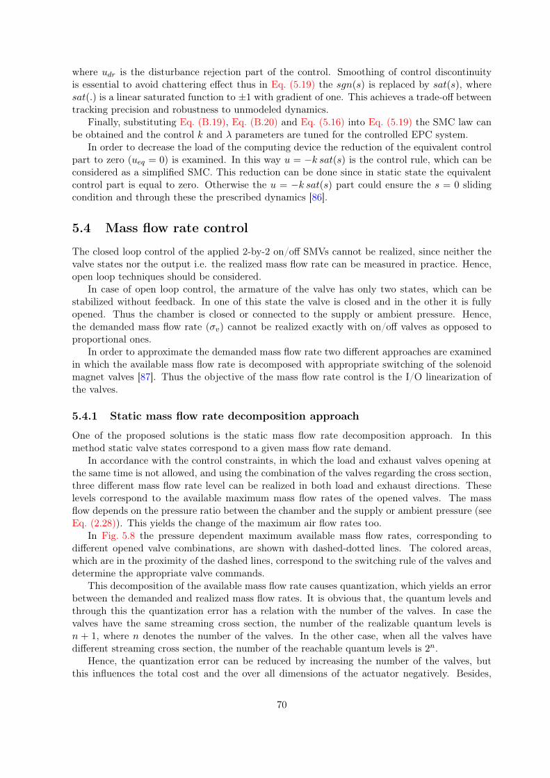
where udr is the disturbance rejection part of the control. Smoothing of control discontinuityis essential to avoid chattering effect thus in Eq. (5.19) the sgn(s) is replaced by sat(s), wheresat(.) is a linear saturated function to ±1 with gradient of one. This achieves a trade-off betweentracking precision and robustness to unmodeled dynamics.

Finally, substituting Eq. (B.19), Eq. (B.20) and Eq. (5.16) into Eq. (5.19) the SMC law canbe obtained and the control k and λ parameters are tuned for the controlled EPC system.

In order to decrease the load of the computing device the reduction of the equivalent controlpart to zero (ueq = 0) is examined. In this way u = −k sat(s) is the control rule, which can beconsidered as a simplified SMC. This reduction can be done since in static state the equivalentcontrol part is equal to zero. Otherwise the u = −k sat(s) part could ensure the s = 0 slidingcondition and through these the prescribed dynamics [86].

5.4 Mass flow rate control

The closed loop control of the applied 2-by-2 on/off SMVs cannot be realized, since neither thevalve states nor the output i.e. the realized mass flow rate can be measured in practice. Hence,open loop techniques should be considered.

In case of open loop control, the armature of the valve has only two states, which can bestabilized without feedback. In one of this state the valve is closed and in the other it is fullyopened. Thus the chamber is closed or connected to the supply or ambient pressure. Hence,the demanded mass flow rate (σv) cannot be realized exactly with on/off valves as opposed toproportional ones.

In order to approximate the demanded mass flow rate two different approaches are examinedin which the available mass flow rate is decomposed with appropriate switching of the solenoidmagnet valves [87]. Thus the objective of the mass flow rate control is the I/O linearization ofthe valves.

5.4.1 Static mass flow rate decomposition approach

One of the proposed solutions is the static mass flow rate decomposition approach. In thismethod static valve states correspond to a given mass flow rate demand.

In accordance with the control constraints, in which the load and exhaust valves opening atthe same time is not allowed, and using the combination of the valves regarding the cross section,three different mass flow rate level can be realized in both load and exhaust directions. Theselevels correspond to the available maximum mass flow rates of the opened valves. The massflow depends on the pressure ratio between the chamber and the supply or ambient pressure (seeEq. (2.28)). This yields the change of the maximum air flow rates too.

In Fig. 5.8 the pressure dependent maximum available mass flow rates, corresponding todifferent opened valve combinations, are shown with dashed-dotted lines. The colored areas,which are in the proximity of the dashed lines, correspond to the switching rule of the valves anddetermine the appropriate valve commands.

This decomposition of the available mass flow rate causes quantization, which yields an errorbetween the demanded and realized mass flow rates. It is obvious that, the quantum levels andthrough this the quantization error has a relation with the number of the valves. In case thevalves have the same streaming cross section, the number of the realizable quantum levels isn + 1, where n denotes the number of the valves. In the other case, when all the valves havedifferent streaming cross section, the number of the reachable quantum levels is 2n.

Hence, the quantization error can be reduced by increasing the number of the valves, butthis influences the total cost and the over all dimensions of the actuator negatively. Besides,

70

pch [Pa]

σdem

v[k

g/s

]

psuppamb 2 3 4 5 6 7 8 9

0

σmaxsl+bl

σmaxbl

σmaxsl

σmaxse+be

σmaxbe

σmaxse

0.005

0.01

−0.005

−0.01

−0.015

uslv = 1; ubl

v = 1; usev = 0; ube

v = 0

uslv = 0; ubl

v = 1; usev = 0; ube

v = 0

uslv = 1; ubl

v = 0; usev = 0; ube

v = 0

uslv = 0; ubl

v = 0; usev = 1; ube

v = 1

uslv = 0; ubl

v = 0; usev = 0; ube

v = 1

uslv = 0; ubl

v = 0; usev = 1; ube

v = 0

uslv = 0; ubl

v = 0; usev = 0; ube

v = 0

Figure 5.8: Available mass flow rates plotted against different chamber pressure

the update rate of the valve commands should be high enough in order to the keep a goodsystem controllability. But increasing the update rate of the valve commands yields increasingcomputation costs and reducing lifetime as well.

With this approach a trade-off must be taken between the number of the valves, the maximumlevel of the mass flow rate, the realizable accuracy and the update rate of the valve commands.

5.4.2 Dynamic mass flow rate decomposition approach

The other proposed solution is a dynamic mass flow rate decomposition approach, in whichdynamic valve states correspond to a given mass flow rate demand. In this approach a lowfrequency PWM method is used, where the switching frequency is low compared to the frequencyrequired for current control.

From the first mean value theorem for integration the mean mass flow rate (σT ) of a valveduring a period T is as follows:

σT =1

T

T∫

0

σ(t) dt. (5.20)

In case of an ideal switching valve, where the switching transients are instantaneous and the

71

realizable mass flow rates are zero and maximal (σ(t) ∈ 0, σm(t)), the mean mass flow rate fora given T period is written as follows:

σT =1

T

ts∫

0

σm(t) dt, (5.21)

where the switch duration ts, is the product of the smallest switching time step tq > 0 and thestep counter i hence, ts = i · tq. In case of constant σm(t) the mean mass flow rate is proportionalto the duty cycle (ts/T ) and it is written as follows: σT = ts/T · σm.

Considering successive valve activation, which means that an additional valve is activatedonly, when the previous one is opened fully, the realizable number of the mass flow rate quantumlevels, is q = n · tq/T + 1 in case of n valves.

In Fig. 5.9 the mass flow rates of an ideal on/off-, a proportional- and a real on/off valveare shown using t k−1

s and t ks switching times (continuous lines) and τ k−1s and τ k

s switchingtimes (dashed lines). It can be seen that the mean mass flow rate of the ideal on/off- and theproportional valves for T period are equal each other as opposed to the real on/off valve. Hence,the mean mass flow rate is not proportional to ts/T due to the valve nonlinearity. Thus, theappropriate switching time of a real on/off valve corresponding to a given mass flow rate shouldbe calculated in a different way.

(k−2)T (k−1)T kT

σ[k

g/s]

time [s]

ideal on/off proportional real on/off

tk−1s tk

s

τk−1s τk

s

σm

σts

T

στs

T

Figure 5.9: Mass flow rates of ideal, proportional and real valves

The switching dynamics of the real valve and through this the piecewise continuous massflow rate is dependent not only on the valve switching time, but on the valve state variables

72

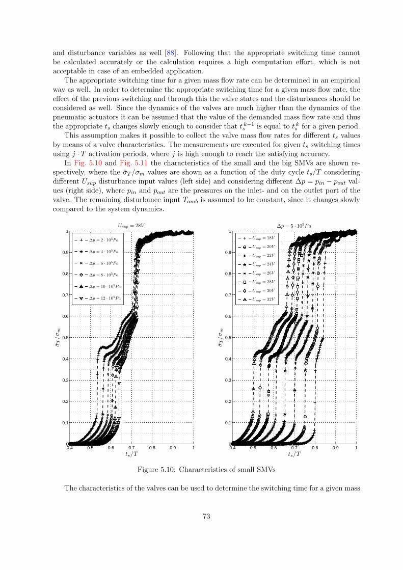
and disturbance variables as well [88]. Following that the appropriate switching time cannotbe calculated accurately or the calculation requires a high computation effort, which is notacceptable in case of an embedded application.

The appropriate switching time for a given mass flow rate can be determined in an empiricalway as well. In order to determine the appropriate switching time for a given mass flow rate, theeffect of the previous switching and through this the valve states and the disturbances should beconsidered as well. Since the dynamics of the valves are much higher than the dynamics of thepneumatic actuators it can be assumed that the value of the demanded mass flow rate and thusthe appropriate ts changes slowly enough to consider that t k−1

s is equal to t ks for a given period.This assumption makes it possible to collect the valve mass flow rates for different ts values

by means of a valve characteristics. The measurements are executed for given ts switching timesusing j · T activation periods, where j is high enough to reach the satisfying accuracy.

In Fig. 5.10 and Fig. 5.11 the characteristics of the small and the big SMVs are shown re-spectively, where the σT /σm values are shown as a function of the duty cycle ts/T consideringdifferent Usup disturbance input values (left side) and considering different ∆p = pin − pout val-ues (right side), where pin and pout are the pressures on the inlet- and on the outlet port of thevalve. The remaining disturbance input Tamb is assumed to be constant, since it changes slowlycompared to the system dynamics.

0.4 0.5 0.6 0.7 0.8 0.9 10

0.1

0.2

0.3

0.4

0.5

0.6

0.7

0.8

0.9

1

σT/σ

m

ts/T

Usup = 28V

∆p = 2 · 105Pa

∆p = 4 · 105Pa

∆p = 6 · 105Pa

∆p = 8 · 105Pa

∆p = 10 · 105Pa

∆p = 12 · 105Pa

0.4 0.5 0.6 0.7 0.8 0.9 10

0.1

0.2

0.3

0.4

0.5

0.6

0.7

0.8

0.9

1

σT/σ

m

ts/T

∆p = 5 · 105Pa

Usup = 18V

Usup = 20V

Usup = 22V

Usup = 24V

Usup = 26V

Usup = 28V

Usup = 30V

Usup = 32V

Figure 5.10: Characteristics of small SMVs

The characteristics of the valves can be used to determine the switching time for a given mass

73

0.4 0.5 0.6 0.7 0.8 0.9 10

0.1

0.2

0.3

0.4

0.5

0.6

0.7

0.8

0.9

1σ

T/σ

m

ts/T

Usup = 28V

∆p = 2 · 105Pa

∆p = 4 · 105Pa

∆p = 6 · 105Pa

∆p = 8 · 105Pa

∆p = 10 · 105Pa

∆p = 12 · 105Pa

0.4 0.5 0.6 0.7 0.8 0.9 10

0.1

0.2

0.3

0.4

0.5

0.6

0.7

0.8

0.9

1

σT/σ

m

ts/T

∆p = 5 · 105Pa

Usup = 18V

Usup = 20V

Usup = 22V

Usup = 24V

Usup = 26V

Usup = 28V

Usup = 30V

Usup = 32V

Figure 5.11: Characteristics of big SMVs

flow rate as follows:ts = T · f(σT /σm,∆p, Usup). (5.22)

Since the cross section of the big SMVs is much higher than the cross section of the smallones the big valve is not used alone. Instead, the small SMV switching is applied in the lowrange of the mass flow rate demand and if the mass flow rate demand is higher than the availablemaximum mass flow rate of the small SMV, the small SMV is opened fully and the big SMVswitching is applied additionally. Thus the big SMV switching without applying the small oneis not used.

To allow the calculation of the switching time for arbitrary mass flow rate demand anddisturbances, interpolation is used between the measured points. Moreover, the computationcost can be kept at a low level in case of using look-up tables and linear interpolation. Besides,the update rate of the valve commands can be decreased compared to the previous method,since the quantization error is decreased. This provides a method better suited for embeddedenvironment application.

5.5 State observer

During the development of an observer, on one hand, the estimation error and on the other handthe computational cost and the memory claim should be considered. Since these are conflicting

74

criteria, a trade-off between them should be found.The simplest way to estimate the velocity state is to apply the Euler finite differential method

on the position state. Through this the first derivative of the signal can be achieved, which isthe velocity. This approach offers low computational cost, but in presence of noise the estimatedvelocity becomes very noisy and unsuitable for feedback.

Since the system is highly nonlinear, linear observer design methods such as the Luenbergeror Kalman filtering neither can be used. Although many state estimation methods are elaboratedand applied for nonlinear systems, e.g. extended Kalman filtering [89], model based open loopstate observer [90] and feedback linearization based observer [91] these have problems with theapplication for the EPC model because the input of the model is not known exactly and themodel has parametric uncertainties as well.

This problem could be overcome with the H∞ filtering [92], which can handle both of theinput and the parameter uncertainties of the model, but the performance of the filter is decreasedsignificantly if the uncertainties are increased. Moreover, the computational cost of this estima-tion method does not allow its use in embedded application. Hence, an appropriate method,which does not require the model input and has low computational cost should be found.

High-gain observers play an important role in the design of output feedback control of feed-back linearizable systems. To illustrate this role without complications, let us consider the specialcase of a SISO nonlinear system which has a uniform relative degree equal to the dimension ofthe state vector. Such a system has no zero dynamics and can be transformed into the normalform (see details in [40]).

x = Ax+B [a (x)u+ b (x)]

y = Cx, (5.23)

where (A, B, C) are canonical form matrices which represent a chain of n integrators.Suppose u = ψ(x, t) is a state feedback control that meets the design objectives over a certain

domain. To implement this control using output feedback, an observer is used as follows:

˙x = Ax+B [a0 (x)ψ(x, t) + b0 (x)] +H (y −Cx) , (5.24)

where a0 (x) and b0 (x) are nominal models of the nonlinear functions a (x) and b (x) respectively,and the n × 1 matrix H is the observer gain. The output feedback control is taken as ψ(x, t).It is shown in [93, 94] that the output feedback control recovers the performance achieved understate feedback when the observer gain H is chosen as

H =[ α1

ǫ

α2

ǫ2. . .

αn

ǫn

]

, (5.25)

where ǫ is a small positive parameter and the positive constants αi are chosen such that the rootsof

sn + α1sn−1 + . . .+ αn−1s+ αn = 0 (5.26)

have negative real parts. This choice of H assigns the eigenvalues of (A − HC) at 1/ǫ timesthe roots of Eq. (5.26). It is shown in [93] that the estimation error will decay to O(ǫ) valuesafter a short transient period [0, T1(ǫ)] where T1(ǫ) tends to zero as ǫ tends to zero. Duringthis transient period, the estimate x may exhibit peaking behavior where the transient responsetakes impulsive-like form. This peaking phenomenon can be overcome by saturating the controlor the state estimates outside a compact region of interest.

The observer equation Eq. (5.24) is nonlinear due to the terms a0ψ and b0. Choosing thenominal functions a0, and b0 to be zero, which corresponds to uncertain a and b functions anduncertain inputs, results in a linear high-gain observer as follows:

˙x = Ax+H (y −Cx) . (5.27)

75

In this way the terms of the Eq. (5.23) obtained as follows:

A =

0 1 00 0 10 0 0

, B =

001

, C = [ 0 0 1 ] ,

a (x) = LgL2fh(x) and b (x) = L3

fh(x).

The a (x), b (x) and u parts can be left out, since a (x) and b (x) are highly nonlinear and haveuncertain parameters as well, moreover the input u is not known exactly as mentioned above.With this assumption the relation of the linear high-gain observer Eq. (5.27) can be realized.Hence, the transfer function from y to x is written as follows

G(s) = (sI−A+HC)−1H. (5.28)

Thus, for the EPC

G(s) =1

d (ǫs)

α1ǫ2s2 + α2ǫs+ α3

α2ǫs2 + α3sα3s

2

, (5.29)

where d (ǫs) = ǫ3s3 + α1ǫ2s2 + α2ǫs+ α3.

The parameters of the observer are chosen as follows: ǫ = 0.0025, α1 = 5, α2 = 2.5 andα3 = 1. With these parameters the system matrix in Eq. (5.28) is remained Hurwitz and thecut off frequency of the HGO becomes two decades higher than the cut off frequency of the EPClinearized models for different equilibrium points [95]. The magnitude and phase of the frequencyresponse of the HGO and the EPC linearized models are shown in Fig. 5.12.

5.6 Experimental results

The verification of the developed controls are performed by extensive simulations using theMATLAB/SIMULINK environment. Then the best control method is chosen to extend it withthe developed state observer and further tested on a real clutch bench. Finally, the performanceof the observer based feedforward/feedback control is demonstrated on a test vehicle.

The aim of the performance test is to demonstrate the behavior of the designed controllers.Thus, the system performance indexes correspond to the reference position tracking capabilityof the closed loop systems.

Two test sequences, which cover typical clutch applications, are chosen to examine the track-ing capability. First, two steps with 100% stroke are applied to derive the settling times, thenengagement test functions are used to get the settling times of the slipping phases and catchcritical overshoots.

Four different lengths of time are distinguished according to the starting and reaching strokesduring a step-response. The resulted time factors are the arithmetic mean of the correspondingmeasured times of the two steps. The starting and reaching strokes are noted in the factorssubscript (Txx−xx%).

Six engagement slopes are tested afterwards. Each of them starts from 100% stroke andjumps down immediately to 70%, 60%, 50%, 40%, 30% and 20% respectively, then followedby a linear ramp, which lasts 2s and descends 20% stroke during this stretch of time. Thetime duration of reaching a 5% environment of the demanded slope is measured separately foreach ramp (T1 − T6). Moreover, the critical overshoots, i.e. the positive errors in the clutchengagement domain, (s1 − s6) during the slopes are captured. The graphical interpretation ofthese performance indices are shown in Fig. 5.13.

76

−100

−50

0

50

yto

x

Mag

[dB

]

EPC HGO

−300

−200

−100

0

yto

x

Phase

[deg

]

0

20

40

60

yto

˙ x

Mag

[dB

]

−100

0

100

yto

˙ x

Phase

[deg

]

0

50

100

yto

¨ x

Mag

[dB

]

100

101

102

103

104

−100

0

100

200

yto

¨ x

Phase

[deg

]

Frequency [rad/s]

Figure 5.12: Magnitude and phase of the frequency response from y to x, ˙x and to ¨x

Besides the time factors and overshoots, the tracking errors are evaluated for both of the twosequences in L2 norm as:

|ǫ|2 =

√

1

T

∫ T

0

(xref (t)− xpst(t)

xref

)2

dt, (5.30)

where the overline refers to the integral mean of the reference signal and T is the duration of thetest case.

Finally the measure of the reference position tracking capability is defined by

χ =1

√∑18

i=1wiχ2i

, (5.31)

where χi corresponds to the performance indexes above (Txx, sx and |ǫ|2). Moreover, in order

77

0 0.2 0.4 0.6 0.8 1 1.2 1.4 1.6 1.8 20

20

40

60

80

100

xpst

[%]

time [s]

xref

xpst

xref − xpst

0 2 4 6 8 10 12 14 16 180

20

40

60

80

100

xpst

[%]

time [s]

T0−5%

T0−95%

T100−95%

T100−5%

T1

T2

T3

T4

T5

T6

s1

s2

s3

s4

s5

s6

Figure 5.13: Graphical interpretation of the performance indices

to achieve the weighted sum of the individual squared numbers wi weights are used (see detailslater).

5.6.1 Simulation test

To obtain the simulation results the stiff ODE15s solver with variable step size is used, where therelative tolerance of the solver is set up to 10−8. While the model runs at base sampling rate, theposition control is placed into an atomic subsystem, with 5ms fixed step size. In the preliminarytests 10ms update rate is considered also, but in this way the control loop has too much delayand cannot stabilize the system. Since the dynamics of the applied sensors are much higher thanthe dynamics of the EPC system the delay of the sensors are neglected. The parameter valuesconsidered in software-in-the-loop (SIL) tests, can be seen in Tab. A.1.

In the first step, the simplified model M2 is used as the controlled plant to achieve anappropriate environment for quick controller tuning. Hence, the feedback controls (LQ, SMC,H∞) are tested only.

After some trials a trade-off between the performance and the stability is taken for all thethree controls. The time graph of the step response test, in case of the M2 model, is shown inFig. 5.14, while the time graph of the engagement test is shown in Fig. 5.15.

78

0 1 2 3 4 5 6 7 8 9−0.02

0

0.02

σv

[kg/

s]

σmin, σmax

0 1 2 3 4 5 6 7 8 90

5x 10

5

pch

[Pa]

0 1 2 3 4 5 6 7 8 90

50

100

xpst

[%]

xref LQ H∞ SMC

0 1 2 3 4 5 6 7 8 9−5−3

0

35

ǫ[%

]

time [s]

Figure 5.14: Step responses with 100% stroke in case of simplified model

0 2 4 6 8 10 12 14 16 18−0.02

0

0.02

σv

[kg/

s]

σmin, σmax

0 2 4 6 8 10 12 14 16 180

5x 10

5

pch

[Pa]

0 2 4 6 8 10 12 14 16 180

50

100

xpst

[%]

xref LQ H∞ SMC

0 2 4 6 8 10 12 14 16 18−5−3

0

35

ǫ[%

]

time [s]

Figure 5.15: Clutch engagement test functions in case of simplified model

79

The performance indexes are gathered in Tab. 5.1. When calculating the reference positiontracking capability χ, the following weights are used: wi = 1 i = 1 . . . 4, 6 . . . 11 in case ofreaching times (Txx), wi = 0.75 i = 12 . . . 17 in case of overshoots (sx) and wi = 0.01 i = 5, 18in case of tracking errors (|ǫ|x).

From the tests it can be seen that the LQ control cannot fulfill the requirements regardingthe response times T1-T4. Hence, the LQ control is not appropriate for advanced clutch control.The SMC has the best performance during the SIL tests. Although the H∞ controller has alsoappropriate performance, it has not tested furthermore, since it has much larger computationalcost than the SMC. This comes on one hand from the feedback linearization and on the otherhand from the 5 th order nature.

In the second step, the SMC is tested using the detailed nonlinear dynamic hybrid modelM0 of the clutch system. In this case not only the position control, but the mass flow ratecontrol is integrated into the closed loop system.

In order to obtain the best solution, both the static and dynamic mass flow rate decompositionapproaches are tested. Moreover, in case of the static mass flow rate decomposition approachthe control system is tested not only with 5ms but with 1ms update rate as well, since theupdate rate has a high influence to the accuracy and the stability of the closed loop system. Inthe other case, the dynamic mass flow rate is run with 5ms update rate. This means that thedynamic mass flow rate controller can get the desired mass flow rate in every 5ms and providesthe appropriate opening time accordingly. The resolution of the opening time is 1µs.

The time graph of the step response test, in case of model M0, is shown in Fig. 5.16, whilethe time graph of the engagement test is shown in Fig. 5.17. In these tests SMC1 and SMC2

correspond to static mass flow rate decomposition with 5ms and 1ms update rate respectively,while SMC3 corresponds to dynamic mass flow rate decomposition with 5ms update rate. Theperformance indexes are gathered in Tab. 5.1 as well.

Table 5.1: Performance indices of step response and clutch slipping tests

Simplified model Detailed model Test b.

Nr. χi wi Spec. LQ H∞ SMC SMC1 SMC2 SMC3 SMC4 Unit

1 T0−95% 1 0.2 0.200 0.190 0.168 0.220 0.192 0.156 0.198 s

2 T100−95% 1 0.04 0.029 0.025 0.025 0.022 0.024 0.027 0.032 s

3 T0−5% 1 0.04 0.031 0.018 0.015 0.028 0.021 0.022 0.030 s

4 T100−5% 1 0.5 0.458 0.446 0.445 0.369 0.345 0.348 0.399 s

5 |ǫ|2

0.01 6 6.36 5.91 5.97 5.85 5.64 5.71 5.70 -

6 T1 1 0.1 0.161 0.080 0.062 0.059 0.057 0.057 0.042 s

7 T2 1 0.13 0.193 0.092 0.074 0.134 0.112 0.076 0.057 s

8 T3 1 0.15 0.217 0.099 0.086 0.146 0.122 0.125 0.067 s

9 T4 1 0.2 0.243 0.110 0.099 0.191 0.139 0.134 0.084 s

10 T5 1 0.3 0.268 0.146 0.145 0.274 0.182 0.184 0.116 s

11 T6 1 0.4 0.284 0.231 0.230 0.323 0.209 0.209 0.200 s

12 s1 0.75 3 0.0 0.0 0.1 2.4 2.0 0.3 1.8 %

13 s2 0.75 3 0.0 0.0 0.0 0.4 0.0 0.2 1.3 %

14 s3 0.75 3 0.0 0.0 0.0 0.0 0.0 0.0 1.4 %

15 s4 0.75 3 0.0 0.0 0.0 0.0 0.0 0.0 1.3 %

16 s5 0.75 3 0.0 0.0 0.0 0.0 0.0 0.0 0.3 %

17 s6 0.75 3 0.0 0.0 0.0 0.0 0.0 0.0 0.0 %

18 |ǫ|2

0.01 3 2.24 1.94 1.90 2.01 1.87 1.91 1.98 -

χ 0.16 0.99 1.16 1.18 0.44 0.53 1.18 0.38 -

80

0 1 2 3 4 5 6 7 8 9−0.02

0

0.02

σv

[kg/

s]

σmin, σmax

0 1 2 3 4 5 6 7 8 90

5x 10

5

pch

[Pa]

0 1 2 3 4 5 6 7 8 90

50

100

xpst

[%]

xref SMC1 SMC2 SMC3

0 1 2 3 4 5 6 7 8 9−5−3

0

35

ǫ[%

]

time [s]

Figure 5.16: Step responses with 100% stroke in case of detailed model

0 2 4 6 8 10 12 14 16 18−0.02

0

0.02

σv

[kg/

s]

σmin, σmax

0 2 4 6 8 10 12 14 16 180

5x 10

5

pch

[Pa]

0 2 4 6 8 10 12 14 16 180

50

100

xpst

[%]

xref SMC1 SMC2 SMC3

0 2 4 6 8 10 12 14 16 18−5−3

0

35

ǫ[%

]

time [s]

Figure 5.17: Clutch engagement test functions in case of detailed model

81

As can be seen from the results the SMC1 cannot fulfill the requirements, due to the stepresponse settling time and the accuracy. Although the SMC2 has better performance it requirestoo high update rate for embedded application. The SMC3 control has the best performancejust like in case of simplified model. Thus this control and through this the dynamic mass flowrate approach is proposed for further assessment in real environment.

5.6.2 Clutch bench test

In this phase the real actuator with the selected position and mass flow rate control is testedon a clutch test bench. In order to feed the controls with all the states the designed high-gainobserver is integrated into the control algorithm as well, marked as SMC4.

The layout of the test bench is shown in Fig. 5.18. For the HIL test an electro-pneumaticClutch Actuator Unit (CAU) with valve module and central release bearing is used.

Figure 5.18: Electro-pneumatic clutch system layout

The actuator is provided with a position sensor to measure the current position of the piston,which has a direct connection to the release bearing. Besides, a pressure sensor is connectedto the chamber to measure the current pressure. The CAU is supplied from an air reservoir,whose nominal pressure level is 9.5bar (abs). The supply voltage is set to 28V . An acquisitionPC is used to provide the reference signal for the Clutch Control Unit (CCU). Hence one getsan electro-pneumatically actuated Clutch-By-Wire system, which lets one to adjust the clutchposition/torque arbitrary. Thus the reference signal (xref ) is one of the input of the CCU.Besides, the CCU gets the current position (xpst), which is the feedback signal from the CAU.

The CCU has analogue-to-digital converters with 12bit resolution and has a 16bit fixed pointarithmetics, hence the effect of the quantization of the signal amplitude is not considerable. Thecontrol is run with 5ms update rate and has 1µs actuation time resolution similarly as in caseof simulation.

The CCU outputs are the control signal of the valves (uxxv ). The valves and the power stagesare integrated into the CAU. The actuator force acts against the load (Fl) and drives the ClutchMechanism (CM) to the demanded position.

During the HIL test the same test cases are used as before. The time graph of the stepresponse test in case of bench test, is shown in Fig. 5.19, while the time graph of the engagementtest is shown in Fig. 5.20. Moreover, the sliding surface and the state trajectory in the phaseplane during a step response is shown in Fig. 5.21. Starting from the initial condition, the statetrajectory reaches the sliding surface in a finite time, and then slides along the surface towards

82

0 1 2 3 4 5 6 7 8 9−0.02

0

0.02

σv

[kg/

s]

σmin, σmax

0 1 2 3 4 5 6 7 8 90

5x 10

5

pch

[Pa]

0 1 2 3 4 5 6 7 8 90

50

100

xpst

[%]

xref SMC4

0 1 2 3 4 5 6 7 8 9−5−3

0

35

ǫ[%

]

time [s]

Figure 5.19: Step responses with 100% stroke in case of test bench

0 2 4 6 8 10 12 14 16 18−0.02

0

0.02

σv

[kg/

s]

σmin, σmax

0 2 4 6 8 10 12 14 16 180

5x 10

5

pch

[Pa]

0 2 4 6 8 10 12 14 16 180

50

100

xpst

[%]

xref SMC4

0 2 4 6 8 10 12 14 16 18−5−3

0

35

ǫ[%

]

time [s]

Figure 5.20: Clutch engagement test functions in case of test bench

83

−0.01

−0.005

0

0.005

0.01

−1

−0.5

0

0.5

1−100

−50

0

50

100

x [m]˙x

[

ms

]

¨ x[

m s2

]

Sliding phase

Reaching phase

Sliding surface

Figure 5.21: The sliding surface and the state trajectory in the phase plane

xd exponentially, with a time-constant equal to 1/λ. The performance indexes are gathered inTab. 5.1 as well.

Although the amplitude of the sensor noise is up to 2% and thus it modifies the values of theovershoots the requirements regarding this factor are fulfilled. Furthermore, the time factors aresimilar to those of the SIL tests. Hence the control algorithm is appropriate for vehicle test.

5.6.3 Vehicle test

For the vehicle test a heavy duty truck, equipped with automated mechanical transmission, isused, hence the reference position comes from the transmission control unit. During the test thevehicle is not loaded so that the driver can better feel the effect of the clutch slipping.

Firstly, the attention is focused to the smooth launch of the vehicle, where a low dynamics,but very accurate position tracking is needed.

In the beginning of the test, the engine is off, the gear box is in neutral gear and the clutchis disengaged (see Fig. 5.22).

In the current test case, when the engine is started (at 0.8s), a touch point learning process isstarted immediately as well. In this phase, the stroke of the clutch actuator, regarding the touchpoint, where the pressure plate reaches the friction disc is determined. When the engine speed(ωe) reaches its idle value, the clutch is engaged immediately. Thus, the input shaft speed of thegearbox (ωg) is brought up to the engine speed (at 1.4s). Then the clutch is disengaged fullyto allow for a second engagement along a ramp (2.3s − 3.9s). When the clutch is disengaged,

84

0 5 10 15 20 250

T

t s[s

]

tsls tbl

stses tbe

s

0 5 10 15 20 250

2

4

6x 10

5

pch[P

a]

0 5 10 15 20 250

50

100

xpst

[%]

xref xpst

0 5 10 15 20 25−5−3

0

35

ǫ[%

]

0 5 10 15 20 250

1000

2000

ω[r

pm

]

time [s]

0 5 10 15 20 250

5

10

v[k

m/h]

ωg ωe v

Figure 5.22: Smooth launch of the vehicle

the input shaft speed starts to decrease till the clutch stroke reaches the touch point. At thetouch point, the gradient of the decrease is changed (at 3.8s), and then the input shaft speedstarts to increase. At the end of the touch point learning process, the learned stroke is checked.Hence, the input shaft speed increases again to reach the engine speed, and then the clutch isdisengaged in order to let input shaft speed drop. The clutch stroke is set to the newly learnedtouch point ( xpst = 40%) along a ramp as well (4.6s − 5.2s). When the stroke reaches it, thegradient of the input shaft speed is changed slightly. In order to find the touch point correctlya very accurate control is needed.

After the successful learning, a smooth vehicle launch is executed. The gearbox is shifted intoan appropriate gear (at 14.2s) and the clutch actuator is set to disengaged state (xpst = 65%).When the driver pushes the accelerator pedal, the reference position jumps immediately to thetouch point (at 19s). Then the clutch is engaged further to reach the appropriate transmittedtorque for the smooth vehicle launch. This phase is one of the most important parts in the clutchcontrol. Since, on one hand, the delay of the touch point reaching time causes unwanted increasein engine speed and through this higher friction disc wear. On the other hand, the overshootcan cause driveline oscillations and through this reduced driver comfort or can stall the engine

85

completely. When the vehicle is launched and the clutch slip is decreased to zero, the clutch isfully engaged (at 23.3s).

A dynamic vehicle launch and gear shifting processes are tested afterwards (see Fig. 5.23).In case of a dynamic start, the reference position jumps immediately to the touch point as well(at 0.8s). Then along a ramp an appropriate torque is set (1.1s − 1.7s). When the vehicle islaunched and the clutch slip is decreased to zero, the clutch is fully engaged again (at 2.6s).

0 2 4 6 8 10 12 14 16 18 200

T

t s[s

]

tsls tbl

stses tbe

s

0 2 4 6 8 10 12 14 16 18 200

2

4

6x 10

5

pch

[Pa]

0 2 4 6 8 10 12 14 16 18 200

50

100

xpst

[%]

xref xpst

0 2 4 6 8 10 12 14 16 18 20−5−3

0

35

ǫ[%

]

0 2 4 6 8 10 12 14 16 18 200

500

1000

1500

2000

ω[r

pm

]

time [s]

0 2 4 6 8 10 12 14 16 18 200

10

20

30

v[k

m/h]

ωg ωe v

Figure 5.23: Dynamic launch and gearshifting

The gearshifting is started with a rapid disengagement (at 6.4s) and with a controlled slipto engage (7s− 7.4s). At higher gears the reference is a step function only.

As seen from the measurement, the error is in the tolerance band (dashed lines). Only whenthe reference changed instantaneously, is the error out of this range. This is the consequence ofthe limited actuator dynamics. Hence, the accuracy of the closed loop system is acceptable.

There are no critical overshoots, the step response times are within the allowed range andthe driver feeling is satisfactory as well.

86

5.7 Summary

In this chapter an observer based feedforward/feedback control of an electro-pneumatic clutchsystem is developed using the previously designed detailed and simplified models of the system.

The control requirements and constraints are defined for the state of the art clutch systems.Using the simplified model, the controller structure is specified. In this cascaded structure thefeedback part corresponds to piston position control, meanwhile the feedforward part correspondsto mass flow rate control and ensures I/O linearization for the solenoid magnet valves.

During the control design different methods are examined for both parts. For piston positioncontrol linear quadratic servo, robust H∞ and nonlinear sliding mode control approaches aredeveloped. For mass flow rate control a static and a dynamic open loop mass flow rate decompo-sition are designed to achieve I/O linearized solenoid magnet valve behavior. Since the appliedcontrol methods require full state feedback, a state observer is designed as well based on thehigh-gain observer design method.

Hence, an LQ servo controller has been designed and tuned for the nonlinear dynamic controloriented model of EPC systems. Based on simulation results it has been found that this type ofcontroller cannot fulfill the dynamic requirements regarding electro-pneumatic clutch control.

A robust H∞ controller, with exact model linearization via state feedback has been designedand tuned afterwards for the nonlinear dynamic control oriented model of EPC systems. Based onsimulation results it has been found that this type of controller fulfills the dynamic requirements.However, this method cannot be applied in the target environment (single core processor 30 −40kHz and 512kilobyte RAM) due to its computational complexity.

A nonlinear type SMC controller has been designed and tuned for the nonlinear dynamiccontrol oriented model of EPC systems. In order to decrease the load of the computing devicethe reduction of the equivalent control part to zero (ueq = 0) is executed. Based on simulationresults it has been found that this type of controller fulfills the dynamic requirements.

The SMC with the dynamic mass flow rate control can fulfill the requirements in case ofsimulation with the detailed nonlinear dynamic hybrid model. For the bench tests the SMC andthe dynamic mass flow rate control is extended with the designed high-gain observer and it hasbeen shown that the requirements have been fulfilled in real environment. Vehicle tests havebeen executed with the designed high-gain observer based cascaded dynamic mass flow rate /sliding mode controller and it has been found that the system can fulfill the requirements andensures good driver comfort.

87

Chapter 6

Conclusions

The main contributions and the proposed theses of this work are summarized in the next sectionof the concluding chapter, then the publications related to this dissertation are listed and finally,the possible directions for further research are given.

6.1 Theses

The relevant chapter of the dissertation and the labels of the related publications (enumeratedin Section 6.2) are indicated in parenthesis.

1. Thesis Nonlinear dynamic hybrid model of electro-pneumatic clutch systems (Chapter 2)([P1])

The nonlinear dynamic hybrid model of electro-pneumatic clutch systems (M0) consideredas a mixed thermodynamical, mechanical and electro-magnetic system has been built andverified using a systematic modeling methodology. It has been shown that the model exhibitsthe following special properties:

i. The nonlinear dynamic hybrid model of electro-pneumatic clutch systems is given bya set of nonlinear ordinary differential-algebraic equations.

ii. It has been shown that the 16 state equations of the nonlinear hybrid dynamic modelcan be written into hybrid nonlinear state-space form.

dx(k)M0

dt= f

(k)M0

(

x(k)M0

, u(k)M0

, d(k)M0

)

,

where k : Rn → N is a piece-wise constant switching function mapping from the state-space to the finite integer set N = 1, 2, . . . 746496. The coordinate function dependsalso on the state vector xM0

, the control input vector uM0and the disturbance vector

dM0.

iii. The model output is linear with respect to the state and disturbance vectors as:

yM0= CM0

xM0+EM0

dM0,

where CM0and EM0

are constant matrices.

iv. It has been shown that the developed model structure is valid for clutch systems appliedwith concentric and forked lever type electro-pneumatic clutch actuators as well, onlythe values of model parameters differ from each other.

88

2. Thesis Simplification of the electro-pneumatic clutch model (Chapter 3)([P2])

A systematic model simplification method has been applied to the nonlinear dynamic hybridmodel of electro-pneumatic clutch systems to obtain a lower order model suitable for controldesign purposes (M2).

The obtained simplified model for control design purposes has the following properties:

i. The dimension of the state vector has been reduced from 16 to 3. The dimension of thecontrol input vector has been reduced from 4 to 1. The dimension of the disturbancevector has been cut to 2 from the original 5, while the output vector has been reducedfrom 8 to 2. The number of the parameters has been reduced from 83 to 8.

ii. All retained system variable entries have preserved their physical meaning.

iii. The discrete switching terms have been eliminated completely.

iv. The control oriented model has been rewritten into standard input affine state-spaceform as:

dxM2

dt= fM2

(xM2, dM2

) + gM2(xM2

, dM2)u.

The coordinate functions depend on the state vector xM2and the disturbance vector

dM2.

v. The retained disturbance variables are not measured thus the output equation is writ-ten as follow:

yM2= CM2

xM2,

where CM2is a constant matrix.

3. Thesis Dynamic properties of the control oriented electro-pneumatic clutch model(Chapter 4)([P3])

The dynamic properties of the control oriented electro-pneumatic clutch model has beenanalyzed. It has been shown that the model exhibits the following dynamic properties:

i. The control oriented model is jointly controllable and observable with the selectedinput and output, hence the model is minimal.

ii. The zero dynamics is asymptotically stable, since the model has a maximum relativedegree r = n.

iii. The control oriented model is uniformly globally asymptotically stable. The globalasymptotic stability depends on model parameters. The stability criterion is obtainedas follows:

d

dxpstFl(x

∗pst) +

p∗chA2pst

V dch +Apstx∗pst

> 0.

iv. The model parameters and disturbance inputs can be arranged to the following listaccording to the sensitivity of the states variables, regarding the change of these modelcomponents: Apst, V d

ch, pmab, Tamb, mpst and kpst.

4. Thesis Specification of the clutch control problem and design of an observer based cascadedfeedforward/feedback controller for electro-pneumatic clutch systems (Chapter 5)([P4],[P5],[P6],[P7],[P8],[P9],[Pa],[Pb])

The control requirements and constraints have been defined for the state of the art clutch

89

systems. Based on the system model an observer based cascaded mass flow rate / pistonposition controller structure has been developed, where the mass flow rate control part pro-vides I/O linearization for the applied on/off solenoid magnet valves and the position controlpart ensures the position tracking, stabilizing and disturbance rejection task. For the esti-mation of the unmeasured state a high-gain observer has been designed to feed both of theposition control and the flow rate control parts. The properties of the closed loop systemsinvestigated by simulation, bench- and vehicle tests have lead to the following observations:

i. A nonlinear type sliding mode controller has been designed and tuned for the nonlin-ear dynamic control oriented model of electro-pneumatic clutch systems. In order todecrease the load of the computing device the reduction of the equivalent control partto zero (ueq = 0) is executed. Based on simulation results it has been found that thesimplified sliding mode controller fulfills the dynamic requirements.

ii. The cascaded dynamic mass flow rate / simplified sliding mode position control canfulfill the requirements in case of simulation with the detailed nonlinear dynamic hybridmodel of electro-pneumatic clutch systems.

iii. For the bench tests the cascaded dynamic mass flow rate / simplified sliding modeposition control is further extended with the designed high-gain observer to get theobserver based feedforward/feedback control structure and it has been shown that therequirements have been fulfilled in real environment as well.

iv. Vehicle tests have been executed with the designed high-gain observer based cascadeddynamic mass flow rate / simplified sliding mode controller and it has been found thatthe system can fulfill the requirements and ensures good driver comfort.

6.2 Publications

6.2.1 Publications directly related to the thesis

[P1] B. Szimandl, H. Németh, Dynamic hybrid model of an electro-pneumatic clutch sys-tem, Mechatronics 23 (1) (2013) 21 – 36. doi:10.1016/j.mechatronics.2012.10.006.(1. Thesis)

[P2] B. Szimandl, H. Németh, Systematic model simplification procedure applied to an electro-pneumatic clutch model, Periodica Polytechnica Transportation Engineering 43 (1) (2014)35–47. doi:10.3311/PPtr.7467. (2. Thesis)

[P3] B. Szimandl, H. Németh, Analysis of an electro-pneumatic clutch model, VSDIA 2014 14thMini Conf. On Vehicle System Dynamics, Identification and Anomalies (3. Thesis)

[P4] B. Szimandl, H. Németh, Pneumatikus mágnesszelepek I/O linearizálása, A Jövő Járműve- Járműipari Innováció 5 (3,4) (2013) 14 – 22. (4. Thesis)

[P5] B. Szimandl, H. Németh, Optimal position control of an electro-pneumatic clutch sys-tem, in: Proceedings of the 11th International Symposium on Advanced Vehicle Control(AVEC’12), Seoul, Korea, 2012, pp. 1 – 6. (4. Thesis)

[P6] B. Szimandl, H. Németh, Robust servo control design for an electro-pneumatic clutchsystem using the H∞ method, in: Mechatronic and Embedded Systems and Applications(MESA), 2014 IEEE/ASME 10th International Conference on, 2014, pp. 1–6.doi:10.1109/MESA.2014.6935526. (4. Thesis)

90

[P7] B. Szimandl, H. Németh, Sliding Mode Position Control of an Electro-Pneumatic ClutchSystem, in: IFAC conf. System, Structure and Control, Vol. 5, Part 1, Grenoble, France,2013, pp. 707–712. doi:10.3182/20130204-3-FR-2033.00019. (4. Thesis)

[P8] B. Szimandl, H. Németh, Observer development for an electro-pneumatic clutch actuator,A Jövő Járműve - Járműipari Innováció 5 (1,2) (2014) 5 – 10. (4. Thesis)

[P9] B. Szimandl, H. Németh, Observer based feedforward/feedback control of an electro-pneumatic clutch system submitted to Control Engineering Practice. (4. Thesis)

6.2.2 Submitted patents

[Pa] B. Trencséni, L. Balogh, H. Németh, B. Szimandl, Method for controlling a clutch.(4. Thesis)

[Pb] B. Trencséni, L. Balogh, H. Németh, B. Szimandl, System and method for controlling aclutch. (4. Thesis)

6.2.3 Other publications

Publications not directly related to this thesis are the following:

[O1] B. Szimandl, H. Németh, Closed loop control of electro-pneumatic gearbox actuator, In:European Control Conference. Budapest, Hungary, 23.08.2009-26.08.2009. pp. 2554-2559.

[O2] B. Szimandl, H. Németh, Observer based closed loop control of electro-pneumatic gearboxactuator, In: FISITA World Automotive Congress 2010. Budapest, Hungary, 30.05.2010-04.06.2010. pp. 3051-3061.

[O3] B. Szimandl, L. Balogh, H. Németh, Electro-Mechanical Brake System Modelling In: I.Zobory (szerk.) VSDIA 2008 11th Mini Conference On Vehicle System Dynamics, Identi-fication and Anomalies. Budapest, Hungary, 10.11.2008-12.11.2008. pp. 435-442.

[O4] B. Szimandl, H. Németh, Parameter sensitivity analysis of energy swing based wheel brakesystem, In: I. Zobory (szerk.) VSDIA 2010 12th Mini Conference On Vehicle SystemDynamics, Identification and Anomalies. Budapest, Hungary, 08.11.2010-10.11.2010. pp.493-500.

[O5] Á. Bárdos, B. Szimandl, H. Németh, Feedforward LQ servo backpressure controller forengine exhaust throttles In: I. Zobory (szerk.) VSDIA 2014 15th Mini Conference OnVehicle System Dynamics, Identification and Anomalies. Budapest, Hungary, 10.11.2014-12.11.2014.

6.3 Directions for future research

The results presented in this thesis are planned to be extended. The extension targets first ofall the controller design and its improvement to cover a wider range of parameter uncertainty.The applied assumptions in case of dynamic hybrid model should be revised in order to furtherincrease the accuracy of this model. Moreover model parameter calibration/identification shouldbe considered in order to increase the accuracy of the developed models. In particular, thefollowing topics are planned for future research.

91

• Consideration of nonlinear model in case of magnetic relation. As the applied currentincreases the effect of the nonlinearity and the hysteresis of the magnetization curveincreases as well, thus this phenomenon should be included into the detailed modeldescription.

• In order to increase the accuracy of the models a detailed model parameter calibra-tion/identification should be executed using special test cases.

• Consideration of wider uncertainty range of the dead volume of the chamber (V dch) and

the stiffness of the clutch mechanism (∂Fl/∂xpst) in order the control system can fulfillthe requirements during the whole lifetime of the clutch.

• Based on Fig. 4.1 it seems that the system has pitchfork bifurcation, since the systemhas three equilibrium point along a trajectory for

d

dxpstFl(x

∗pst) +

p∗chA2pst

V dch +Apstx∗pst

< 0

and one ford

dxpstFl(x

∗pst) +

p∗chA2pst

V dch +Apstx∗pst

> 0.

In order to prove this conjecture an exhaustive bifurcation analysis is needed [96].

• Consideration of wider uncertainty range of SMV parameters. The production of theSMV has spread within a given tolerance limit and this causes parameter uncertainty.The parameter change of the SMV has a large effect on the mass flow rate control,therefore some sort of feedback or long time adaptation should be considered.

92

Bibliography

[1] L. Palkovics, A. Fries, Intelligent electronic systems in commercial vehiclesfor enhanced traffic safety, Vehicle System Dynamics 35 (4-5) (2001) 227–289.doi:10.1076/vesd.35.4.227.2044.

[2] G.-O. Kaasa, M. Takahashi, Adaptive Tracking Control of an Electro-PneumaticClutch Actuator, Modeling, Identification and Control 24 (4) (2003) 217–229.doi:10.4173/mic.2003.4.3.

[3] L. X. Jun, Z. C. Rui, L. H. Bin, Electronic Pneumatic Clutch Control of the Heavy Truckbased on Neural Network PID, in: Vehicular Electronics and Safety, 2006. ICVES 2006.IEEE International Conference on, 2006, pp. 232–235. doi:10.1109/ICVES.2006.371589.

[4] H. Li, L. Chen, A Fuzzy Immune PSD Control Approach to Pneumatic Clutch of HeavyTrucks, in: Fuzzy Systems and Knowledge Discovery, 2007. FSKD 2007. Fourth InternationalConference on, Vol. 2, 2007, pp. 534–539. doi:10.1109/FSKD.2007.35.

[5] H. Sande, T. Johansen, G.-O. Kaasa, S. Snare, C. Bratli, Switched backstepping control ofan electropneumatic clutch actuator using on/off valves, in: American Control Conference,2007. ACC ’07, 2007, pp. 76–81. doi:10.1109/ACC.2007.4282614.

[6] H. Langjord, T. Johansen, J. Hespanha, Switched control of an electropneumatic clutchactuator using on/off valves, in: American Control Conference, 2008, 2008, pp. 1513–1518.doi:10.1109/ACC.2008.4586706.

[7] H. Langjord, T. Johansen, C. Bratli, Dual-mode switched control of an electropneumaticclutch actuator with input restrictions, in: European Control Conference, 2009, 2009, pp.2085–2090.

[8] H. Langjord, T. Johansen, Dual-Mode Switched Control of an ElectropneumaticClutch Actuator, Mechatronics, IEEE/ASME Transactions on 15 (6) (2010) 969–981.doi:10.1109/TMECH.2009.2036172.

[9] A. Grancharova, T. Johansen, Explicit approximate model predictive control of con-strained nonlinear systems with quantized input, in: L. Magni, D. Raimondo, F. All-göwer (Eds.), Nonlinear Model Predictive Control, Vol. 384 of Lecture Notes inControl and Information Sciences, Springer Berlin Heidelberg, 2009, pp. 371–380.doi:10.1007/978-3-642-01094-1_30.

[10] A. Grancharova, T. Johansen, Explicit Model Predictive Control of an ElectropneumaticClutch Actuator Using On-Off Valves and Pulse-width Modulation, in: European ControlConference, 2009, 2009, pp. 4278–4283.

93

[11] A. Grancharova, T. Johansen, Design and Comparison of Explicit Model Predictive Con-trollers for an Electropneumatic Clutch Actuator Using On/Off Valves, Mechatronics,IEEE/ASME Transactions on 16 (4) (2011) 665–673. doi:10.1109/TMECH.2010.2049365.

[12] H. Németh, Nonlinear Modeling and Control for a Mechatronic Protection Valve, Ph.D.Theses, Budapest, Hungary, 2004.

[13] B. Förster, J. Lindner, K. Steinel, W. Stürmer, Kupplungssysteme für schwereNutzfahrzeuge, ATZ - Automobiltechnische Zeitschrift 106 (10) (2004) 878–887.doi:10.1007/BF03221661.

[14] B. Förster, K. Steinel, Kupplungsbetätigungssystem ConAct für Nutzfahrzeuge mit automa-tisierten Schaltgetrieben, ATZ - Automobiltechnische Zeitschrift 109 (2) (2007) 140–146.doi:10.1007/BF03221866.

[15] K. Hangos, I. Cameron, Process modelling and model analysis / K.M. Hangos, I.T. Cameron,Academic Press, San Diego, 2001.

[16] R. Lakner, K. Hangos, I. Cameron, On minimal models of process systems, Chemical Engi-neering Science 60 (4) (2005) 1127 – 1142. doi:10.1016/j.ces.2004.09.074.

[17] P. J. Mosterman, G. Biswas, A comprehensive methodology for building hybridmodels of physical systems, Artificial Intelligence 121 (1-2) (2000) 171 – 209.doi:10.1016/S0004-3702(00)00032-1.

[18] C. Wen, Modeling problems of hybrid event dynamic systems, Simulation Practice andTheory 6 (4) (1998) 413 – 422. doi:10.1016/S0928-4869(97)00014-1.

[19] M. Dogruel, M. A. Adli, Hybrid state approach for modelling electrical and me-chanical systems, Mathematical and Computer Modelling 41 (6-7) (2005) 759 – 771.doi:10.1016/j.mcm.2004.01.006.

[20] K. Hangos, I. Cameron, The formal representation of process system modelling assumptionsand their implications, Computers & Chemical Engineering 21, Supplement (0) (1997) S823– S828. doi:10.1016/S0098-1354(97)87604-1.

[21] K. Hangos, I. Cameron, A formal representation of assumptions in processmodelling, Computers & Chemical Engineering 25 (2-3) (2001) 237 – 255.doi:10.1016/S0098-1354(00)00649-9.

[22] K. Hangos, G. Szederkényi, Z. Tuza, The effect of model simplification assumptions on thedifferential index of lumped process models, Computers & Chemical Engineering 28 (1-2)(2004) 129 – 137. doi:10.1016/S0098-1354(03)00166-2.

[23] K. Hangos, Z. Tuza, Process model structure simplification, Computers & Chemical Engi-neering 23, Supplement (0) (1999) S343 – S346. doi:10.1016/S0098-1354(99)80084-2.

[24] H. Németh, P. Ailer, K. M. Hangos, Nonlinear modelling and model verification of a singleprotection valve, Periodica Polytechnica Ser. Transportation Eng. 30 (1-2) (2002) 69 – 96.

[25] R. D. Zucker, Fundamentals of gas dynamics, 2nd Edition, John Wiley & Sons Inc., NewJerse, 2002.

[26] D. F. Young, T. H. Okiishi, Fundamentals of fluid mechanics, 5th Edition, John Wiley &Sons Inc., New Jerse, 2006.

94

[27] K. Fischer, K. Shenai, Dynamics of power MOSFET switching under unclamped inductiveloading conditions, Electron Devices, IEEE Transactions on 43 (6) (1996) 1007 – 1015.doi:10.1109/16.502137.

[28] L. A. Zadeh, C. A. Desoer, Linear system theory; The state space approach, McGraw-HillNew York, 1963.

[29] M. Branicky, V. Borkar, S. Mitter, A unified framework for hybrid control: model andoptimal control theory, IEEE Transactions on Automatic Control 43 (1) (1998) 31–45.doi:10.1109/9.654885.

[30] H. Németh, L. Palkovics, K. M. Hangos, System identification of an electro-pneumaticprotection valve, Technical Report SCL-001/2003, Computer and Automation ResearchInstitute, Budapest, Hungary.

[31] H. H. Woodson, J. R. Melcher, Electromechanical Dynamics: Part I, John Wiley & SonsInc., 1968.

[32] A. Laub, M. Heath, C. Paige, R. Ward, Computation of system balancing transformationsand other applications of simultaneous diagonalization algorithms, IEEE Transactions onAutomatic Control 32 (1987) 115–122. doi:10.1109/TAC.1987.1104549.

[33] B. Moore, Principal component analysis in linear systems: Controllability, observabil-ity, and model reduction, IEEE Transactions on Automatic Control 26 (1981) 17–32.doi:10.1109/TAC.1981.1102568.

[34] J. Hahn, T. F. Edgar, An improved method for nonlinear model reduction using balancingof empirical gramians, Computers & Chemical Engineering 26 (10) (2002) 1379 – 1397.doi:10.1016/S0098-1354(02)00120-5.

[35] J. Hahn, T. F. Edgar, W. Marquardt, Controllability and observability covariance matricesfor the analysis and order reduction of stable nonlinear systems, Journal of Process Control13 (2) (2003) 115 – 127. doi:10.1016/S0959-1524(02)00024-0.

[36] R. Lakner, I. Cameron, K. Hangos, An assumption-driven case-specific model editor, Com-puters & Chemical Engineering 23 (Supplement 1) (1999) S695 – S698, european Sympo-sium on Computer Aided Process Engineering, Proceedings of the European Symposium.doi:10.1016/S0098-1354(99)80170-7.

[37] A. Leitold, K. M. Hangos, Z. Tuza, Structure simplification of dynamic process models,Journal of Process Control 12 (1) (2002) 69 – 83. doi:10.1016/S0959-1524(00)00062-7.

[38] H. Németh, L. Palkovics, K. M. Hangos, Unified model simplification procedure applied toa single protection valve, Control Engineering Practice 13 (3) (2005) 315 – 326, aerospaceIFAC 2002. doi:10.1016/j.conengprac.2004.03.013.

[39] Y. Hong, H.-W. Park, J.-W. Lee, D.-P. Hong, Simulation of clutch actuation system forcommercial vehicle, International Journal of Precision Engineering and Manufacturing 11 (6)(2010) 839–843. doi:10.1007/s12541-010-0101-5.

[40] A. Isidori, Nonlinear Control Systems, 3rd Edition, Springer-Verlag New York, Inc., Secau-cus, NJ, USA, 1995.

95

[41] S. Sastry, Nonlinear Systems: Analysis, Stability, and Control, Interdisciplinary AppliedMathematics, Springer New York, 1999. doi:10.1007/978-1-4757-3108-8.

[42] H. K. Khalil, Nonlinear Systems, 3rd Edition, Prentice Hall, 2002.

[43] J.-J. E. Slotine, W. Li, Applied Nonlinear Control, Prentice Hall, 1991.

[44] D. Cheng, Analysis of linear systems, Addison-Wesley series in electrical engineering,Addison-Wesley Pub. Co., 1959.

[45] S. Skogestad, I. Postlethwaite, Multivariable Feedback Control: Analysis and Design, JohnWiley & Sons, 2005.

[46] K. Hangos, J. Bokor, G. Szederkényi, Analysis and Control of Nonlinear Process Systems,Advanced Textbooks in Control and Signal Processing, Springer London, 2004.

[47] A. M. LYAPUNOV, The general problem of the stability of motion, International Journalof Control 55 (3) (1992) 531–534. doi:10.1080/00207179208934253.

[48] E. Barbashin, N. Krasovskii, On the stability of motion in the large, Dokl. Akad. Nauk.S.S.S.R. 86 (3) (1952) 453–456.

[49] N. N. Krasovskii, Problems of the theory of stability of motion, English translation: StanfordUniversity Press, Stanford, CA, 1963., 1959.

[50] J. LaSalle, Some extensions of Liapunov’s second method, IRE Transactions on CircuitTheory 86 (3) (1960) 520–527.

[51] V. Chellaboina, A. Leonessa, M. Haddad, Generalized lyapunov and invariant set theoremsfor nonlinear dynamical systems, in: American Control Conference, 1999. Proceedings ofthe 1999, Vol. 5, 1999, pp. 3028–3032. doi:10.1109/ACC.1999.782317.

[52] A. Hurwitz, Ueber die Bedingungen, unter welchen eine Gleichung nur Wurzeln mitnegativen reellen Theilen besitzt, Mathematische Annalen 46 (2) (1895) 273–284.doi:10.1007/BF01446812.

[53] I. S. Gradshteyn, I. M. Ryzhik, Analysis of linear systems §15.715 in Tables of Integrals,Series, and Products, 6th ed., Academic Press, 2000.

[54] F. Alonge, F. D’Ippolito, Design and sensitivity analysis of a reduced-order rotor flux optimalobserver for induction motor control, Control Engineering Practice 15 (12) (2007) 1508 –1519. doi:10.1016/j.conengprac.2007.02.011.

[55] I. Hiskens, Stability of hybrid system limit cycles: application to the compass gait bipedrobot, in: Decision and Control, 2001. Proceedings of the 40th IEEE Conference on, Vol. 1,2001, pp. 774–779 vol.1. doi:10.1109/.2001.980200.

[56] I. Hiskens, Trajectory approximation near the stability boundary, in: Circuits and Systems(ISCAS), Proceedings of 2010 IEEE International Symposium on, 30 2010-June 2, pp. 533–536. doi:10.1109/ISCAS.2010.5537559.

[57] B. D. O. Anderson, J. B. Moore, Optimal Control: Linear Quadratic Methods, CourierCorporation, 2007.

96

[58] H. Kwakernaak, R. Sivan, Linear Optimal Control Systems, John Wiley & Sons, Inc., NewYork, NY, USA, 1972.

[59] D. Hrovat, Survey of advanced suspension developments and related optimal control appli-cations, Automatica 33 (10) (1997) 1781 – 1817. doi:10.1016/S0005-1098(97)00101-5.

[60] Y. Li, X. Liu, G. Xing, Discrete-time LQ optimal control of satellite formations in ellip-tical orbits based on feedback linearization, Acta Astronautica 83 (0) (2013) 125 – 131.doi:10.1016/j.actaastro.2012.10.027.

[61] R. Zhang, R. Lu, Q. Jin, Multivariable design of improved linear quadratic regulation controlfor MIMO industrial processes, ISA Transactions Available online 18 April 2015 (2015) –doi:10.1016/j.isatra.2015.03.010.

[62] A. Liu, Y. Liang, S. Gao, J. Gao, Modified linear quadratic optimal control method andapplication in linear brushless direct current motor, in: Electrical Machines and Systems,2007. ICEMS. International Conference on, 2007, pp. 1829–1834.

[63] H. Wang, H. Zhang, X. Wang, Linear quadratic optimal control for continuous-time stochas-tic systems with single input-delay, in: Control and Decision Conference (CCDC), 2012 24thChinese, 2012, pp. 2821–2828. doi:10.1109/CCDC.2012.6244450.

[64] K. Zhou, J. C. Doyle, K. Glover, Robust and Optimal Control, Prentice-Hall, Inc., UpperSaddle River, NJ, USA, 1996.

[65] O. Sename, P. Gáspár, J. Bokor, Robust Control and Linear Parameter Varying approaches:Application to Vehicle Dynamics, Spinger, 2013. doi:10.1007/978-3-642-36110-4.

[66] J. J. Martinez, O. Sename, A. Voda, Modeling and robust control ofBlu-ray disc servo-mechanisms, Mechatronics 19 (5) (2009) 715 – 725.doi:10.1016/j.mechatronics.2009.02.006.

[67] A. Zin, O. Sename, P. Gáspár, L. Dugard, J. Bokor, Robust LPV-H∞ control for activesuspensions with performance adaptation in view of global chassis control, Vehicle SystemDynamics 46 (10) (2008) 889–912. doi:10.1080/00423110701684587.

[68] C. Poussot-Vassal, O. Sename, L. Dugard, P. Gáspár, Z. Szabó, J. Bokor, A new semi-activesuspension control strategy through LPV technique, Control Engineering Practice 16 (12)(2008) 1519 – 1534. doi:10.1016/j.conengprac.2008.05.002.

[69] M. Jung, K. Glover, U. Christen, Comparison of uncertainty parameterisations for H∞

robust control of turbocharged diesel engines, Control Engineering Practice 13 (1) (2005)15 – 25. doi:10.1016/j.conengprac.2003.12.018.

[70] G. Lee, K. You, T. Kang, K. J. Yoon, J. O. Lee, J. K. Park, Modeling and design of H-Infinity controller for piezoelectric actuator LIPCA, Journal of Bionic Engineering 7 (2)(2010) 168 – 174. doi:10.1016/S1672-6529(09)60198-0.

[71] V. I. Utkin, J. Guldner, J. Shi, Sliding mode control in electromechanical systems, TheTaylor & Francis systems and control book series, Taylor & Francis, London, Philadelphia,PA, 1999.

[72] C. Edwards, S. K. Spurgeon, Sliding Mode Control: Theory and Applications, Taylor &Francis systems and control book series, Taylor & Francis, London, 1998.

97

[73] A. Girin, F. Plestan, X. Brim, A. Glumineau, A 3rd order sliding mode controller based onintegral sliding mode for an electropneumatic system, in: Decision and Control, 2006 45thIEEE Conference on, 2006, pp. 1617–1622. doi:10.1109/CDC.2006.376778.

[74] A. Girin, F. Plestan, X. Brun, A. Glumineau, High-order sliding-mode controllers of an elec-tropneumatic actuator: Application to an aeronautic benchmark, Control Systems Technol-ogy, IEEE Transactions on 17 (3) (2009) 633–645. doi:10.1109/TCST.2008.2002950.

[75] A. Paul, J. Mishra, M. Radke, Reduced order sliding mode control for pneumaticactuator, Control Systems Technology, IEEE Transactions on 2 (3) (1994) 271–276.doi:10.1109/87.317984.

[76] S. Das, B. Bandyopadyay, A. Paul, P. Trivedi, Position control of pneumatic actuator usingsliding mode control in conjunction with robust exact differentiator, in: Control, Automa-tion, Robotics and Embedded Systems (CARE), 2013 International Conference on, 2013,pp. 1–6. doi:10.1109/CARE.2013.6733689.

[77] E. Barth, J. Zhang, M. Goldfarb, Sliding mode approach to PWM-controlled pneumaticsystems, in: American Control Conference, 2002. Proceedings of the 2002, Vol. 3, 2002, pp.2362–2367 vol.3. doi:10.1109/ACC.2002.1023995.

[78] S. Laghrouche, M. Smaoui, F. Plestan, Robust control of electropneumatic actuator by 3rd-order sliding mode, in: Decision and Control, 2004. CDC. 43rd IEEE Conference on, Vol. 4,2004, pp. 4375–4380. doi:10.1109/CDC.2004.1429439.

[79] T. Nguyen, J. Leavitt, F. Jabbari, J. Bobrow, Accurate sliding-mode control of pneumaticsystems using low-cost solenoid valves, Mechatronics, IEEE/ASME Transactions on 12 (2)(2007) 216–219. doi:10.1109/TMECH.2007.892821.

[80] J. L. Musgrave, Linear quadratic servo control of a reusable rocket engine, Journal of Guid-ance, Control, and Dynamics 15 (5) (1992) 1149–1154. doi:10.2514/3.20962.

[81] S. Weerasooriya, D. Phan, Discrete-time LQG/LTR design and modeling of a disk driveactuator tracking servo system, Industrial Electronics, IEEE Transactions on 42 (3) (1995)240–247. doi:10.1109/41.382134.

[82] B. Szimandl, H. Németh, Optimal position control of an electro-pneumatic clutch system, in:Proceedings of the 11th International Symposium on Advanced Vehicle Control (AVEC’12),Seoul, Korea, 2012, pp. 1 – 6.

[83] P. Gáspár, I. Szászi, Robust servo control design using identified models, in: 3rd IFACsymposium on robust control design. ROCOND 2000. Prague, 2000., IFAC, Prague, 2000,p. 6.

[84] M. V. Kothare, P. J. Campo, M. Morari, C. N. Nett, A unified frameworkfor the study of anti-windup designs, Automatica 30 (12) (1994) 1869 – 1883.doi:10.1016/0005-1098(94)90048-5.

[85] B. Szimandl, H. Németh, Robust servo control design for an electro-pneumatic clutchsystem using the H∞ method, in: Mechatronic and Embedded Systems and Appli-cations (MESA), 2014 IEEE/ASME 10th International Conference on, 2014, pp. 1–6.doi:10.1109/MESA.2014.6935526.

98

[86] B. Szimandl, H. Németh, Sliding Mode Position Control of an Electro-Pneumatic ClutchSystem, in: System, Structure and Control, Vol. 5, Part 1, Grenoble, France, 2013, pp.707–712. doi:10.3182/20130204-3-FR-2033.00019.

[87] B. Szimandl, H. Németh, Pneumatikus mágnesszelepek I/O linearizálása, A Jövő Járműve- Járműipari Innováció 5 (3,4) (2013) 14 – 22.

[88] B. Szimandl, H. Németh, Dynamic hybrid model of an electro-pneumatic clutch system,Mechatronics 23 (1) (2013) 21 – 36. doi:10.1016/j.mechatronics.2012.10.006.

[89] P. Bauer, J. Bokor, Development and hardware-in-the-loop testing of an Extended KalmanFilter for attitude estimation, in: Computational Intelligence and Informatics (CINTI), 201011th International Symposium on, 2010, pp. 57–62. doi:10.1109/CINTI.2010.5672274.

[90] B. Szimandl, H. Németh, Observer based closed loop control of electro-pneumatic gearboxactuator, in: FISITA, 2010, 2010, pp. 1–10.

[91] T. Szabo, M. Buchholz, K. Dietmayer, A feedback linearization based observer foran electropneumatic clutch actuated by on/off solenoid valves, in: Control Ap-plications (CCA), 2010 IEEE International Conference on, 2010, pp. 1445–1450.doi:10.1109/CCA.2010.5611125.

[92] P. Seiler, B. Vanek, J. Bokor, G. Balas, Robust H∞ filter design using frequencygridding, in: American Control Conference (ACC), 2011, 2011, pp. 1801–1806.doi:10.1109/ACC.2011.5990748.

[93] F. Esfandiari, H. K. Khalil, Output feedback stabilization of fully linearizable systems, In-ternational Journal of Control 56 (5) (1992) 1007–1037. doi:10.1080/00207179208934355.

[94] A. Saberi, P. Sannuti, Observer design for loop transfer recovery and for uncertaindynamical systems, Automatic Control, IEEE Transactions on 35 (8) (1990) 878–897.doi:10.1109/9.58497.

[95] B. Szimandl, H. Németh, Observer development for an electro-pneumatic clutch actuator,A Jövő Járműve - Járműipari Innováció 5 (1,2) (2014) 5 – 10.

[96] Y. Kuznetsov, Elements of applied bifurcation theory, Vol. 112, Springer Verlag, 2004.doi:10.1007/978-1-4757-3978-7.

99

Appendix A

Figures and Tables

Figure A.1: Friction disc, clutch mechanism and concentric clutch actuator from ZF SACHS

100

Figure A.2: Engine, gearbox and clutch system

Figure A.3: Clutch systems applied with forked lever- (left) and concentric type (right) EPCactuators

101

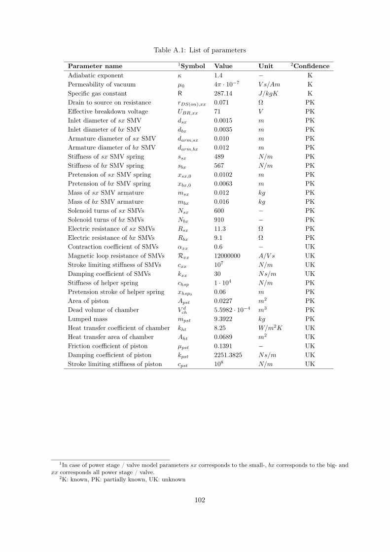
Table A.1: List of parameters

Parameter name 1Symbol Value Unit 2Confidence

Adiabatic exponent κ 1.4 − K

Permeability of vacuum µ0 4π · 10−7 V s/Am K

Specific gas constant R 287.14 J/kgK K

Drain to source on resistance rDS(on),xx 0.071 Ω PK

Effective breakdown voltage UBR,xx 71 V PK

Inlet diameter of sx SMV dsx 0.0015 m PK

Inlet diameter of bx SMV dbx 0.0035 m PK

Armature diameter of sx SMV darm,sx 0.010 m PK

Armature diameter of bx SMV darm,bx 0.012 m PK

Stiffness of sx SMV spring ssx 489 N/m PK

Stiffness of bx SMV spring sbx 567 N/m PK

Pretension of sx SMV spring xsx,0 0.0102 m PK

Pretension of bx SMV spring xbx,0 0.0063 m PK

Mass of sx SMV armature msx 0.012 kg PK

Mass of bx SMV armature mbx 0.016 kg PK

Solenoid turns of sx SMVs Nsx 600 − PK

Solenoid turns of bx SMVs Nbx 910 − PK

Electric resistance of sx SMVs Rsx 11.3 Ω PK

Electric resistance of bx SMVs Rbx 9.1 Ω PK

Contraction coefficient of SMVs αxx 0.6 − UK

Magnetic loop resistance of SMVs Rxx 12000000 A/V s UK

Stroke limiting stiffness of SMVs cxx 107 N/m UK

Damping coefficient of SMVs kxx 30 Ns/m UK

Stiffness of helper spring chsp 1 · 104 N/m PK

Pretension stroke of helper spring xhsp00.06 m PK

Area of piston Apst 0.0227 m2 PK

Dead volume of chamber V dch 5.5982 · 10−4 m3 PK

Lumped mass mpst 9.3922 kg PK

Heat transfer coefficient of chamber kht 8.25 W/m2K UK

Heat transfer area of chamber Aht 0.0689 m2 UK

Friction coefficient of piston µpst 0.1391 − UK

Damping coefficient of piston kpst 2251.3825 Ns/m UK

Stroke limiting stiffness of piston cpst 108 N/m UK

1In case of power stage / valve model parameters sx corresponds to the small-, bx corresponds to the big- andxx corresponds all power stage / valve.

2K: known, PK: partially known, UK: unknown

102

Appendix B

Model transformations

B.1 Linearization around a steady state point x∗

One of the possible ways, to achieve a linear model, is the linearization around a steady statepoint x∗, where x∗ contains the state variables values in a typical equilibrium state. In this waythe model description is in linear time-invariant (LTI) form as follows:

x(t) = Ax(t) +Bu(t)

y(t) = Cx(t) +Du(t),(B.1)

where x ∈ Rn, u ∈ R

r and y ∈ Rm.

The linearization is done by the Jacobian matrix of the system. The x∗ state is determined byexperimental results, where the clutch position reaches the engagement domain. In this domainthe driver is the most sensitive to the transmitted torque.

x∗ =[2.8987 · 105 0 6.071 · 10−3

]. (B.2)

Besides dFl(x∗pst)/dxpst = 2.4 · 104N/m is considered using the characteristics of the clutch

mechanism. With this the state- and input matrices are obtained as follows:

A =∂f (x,d)

∂x

∣∣∣∣x=x∗

=

=

0−p∗chApst

V dch

+Apstx∗pst

0

Apst

mpst−

kpstmpst

−d

dxpstFl(x

∗pst)

mpst

0 1 0

and

(B.3)

B =∂g (x,d)

∂u

∣∣∣∣x=x∗

=

RairTamb

V dch

+Apstx∗pst

0

0

, (B.4)

where A ∈ Rn×n and B ∈ R

n×r.The output matrices are formed as follows:

C =

[

1 0 0

0 0 1

]

and D =

[

0

0

]

, (B.5)

where C ∈ Rm×n and D ∈ R

m×r.

103

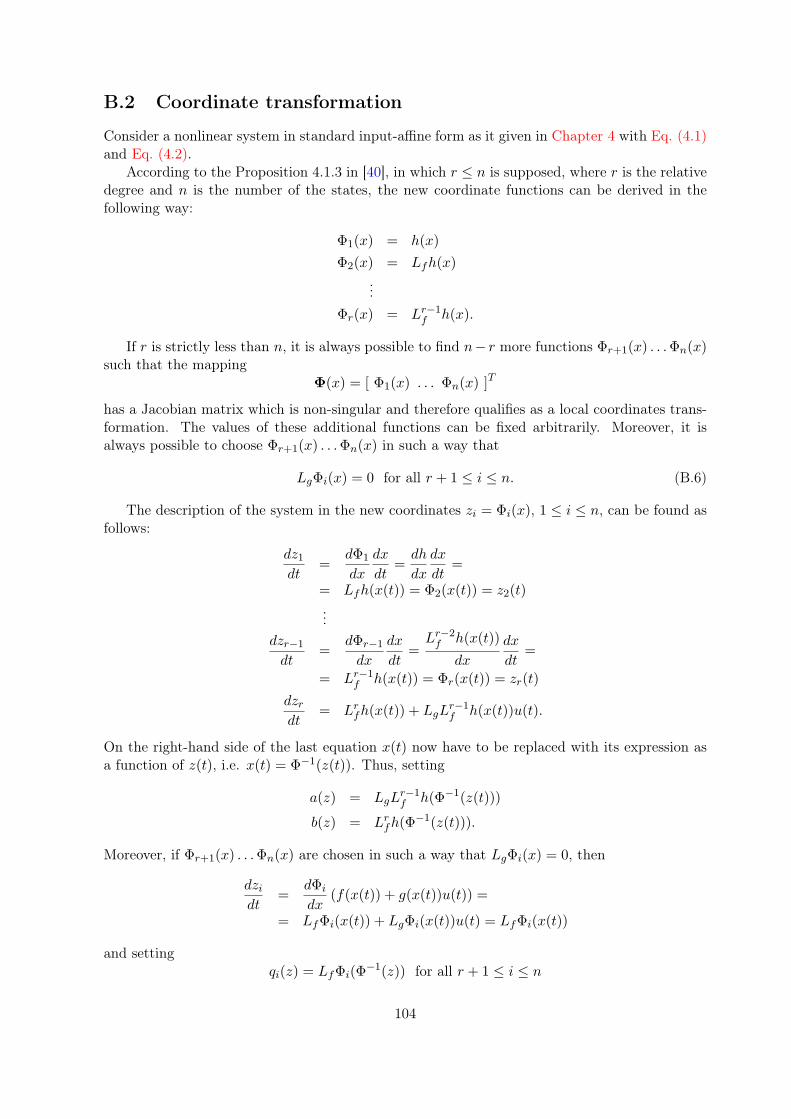
B.2 Coordinate transformation

Consider a nonlinear system in standard input-affine form as it given in Chapter 4 with Eq. (4.1)and Eq. (4.2).

According to the Proposition 4.1.3 in [40], in which r ≤ n is supposed, where r is the relativedegree and n is the number of the states, the new coordinate functions can be derived in thefollowing way:

Φ1(x) = h(x)

Φ2(x) = Lfh(x)

...

Φr(x) = Lr−1f h(x).

If r is strictly less than n, it is always possible to find n− r more functions Φr+1(x) . . .Φn(x)such that the mapping

Φ(x) = [ Φ1(x) . . . Φn(x) ]T

has a Jacobian matrix which is non-singular and therefore qualifies as a local coordinates trans-formation. The values of these additional functions can be fixed arbitrarily. Moreover, it isalways possible to choose Φr+1(x) . . .Φn(x) in such a way that

LgΦi(x) = 0 for all r + 1 ≤ i ≤ n. (B.6)

The description of the system in the new coordinates zi = Φi(x), 1 ≤ i ≤ n, can be found asfollows:

dz1dt

=dΦ1

dx

dx

dt=dh

dx

dx

dt=

= Lfh(x(t)) = Φ2(x(t)) = z2(t)

...

dzr−1

dt=

dΦr−1

dx

dx

dt=Lr−2f h(x(t))

dx

dx

dt=

= Lr−1f h(x(t)) = Φr(x(t)) = zr(t)

dzrdt

= Lrfh(x(t)) + LgL

r−1f h(x(t))u(t).

On the right-hand side of the last equation x(t) now have to be replaced with its expression asa function of z(t), i.e. x(t) = Φ−1(z(t)). Thus, setting

a(z) = LgLr−1f h(Φ−1(z(t)))

b(z) = Lrfh(Φ

−1(z(t))).

Moreover, if Φr+1(x) . . .Φn(x) are chosen in such a way that LgΦi(x) = 0, then

dzidt

=dΦi

dx(f(x(t)) + g(x(t))u(t)) =

= LfΦi(x(t)) + LgΦi(x(t))u(t) = LfΦi(x(t))

and settingqi(z) = LfΦi(Φ

−1(z)) for all r + 1 ≤ i ≤ n

104

then the state-space description of the system in the new coordinates can be obtained as follows:

z1 = z2

z2 = z3...

zr−1 = zr

zr = b(z) + a(z)u (B.7)

zr+1 = qr+1(z)

...

zn = qn(z).

This equations thus defined are said to be in normal form.In order to find the normal form of the EPC model the following coordinate functions are

chosen:

z1 = Φ1(x) = h(x) = xpst (B.8)

z2 = Φ2(x) = Lfh(x) = vpst (B.9)

z3 = Φ3(x) = L2fh(x) = f2 (x,d) = apst. (B.10)

These functions define a transformation z = Φ(x) whose Jacobian matrix

dΦ

dx=

0 0 1

0 1 0

Apst

mpst−

kpstmpst

−d

dxpstFl(xpst)

mpst

, (B.11)

which is non-singular for all x if−Apst/mpst 6= 0. (B.12)

This condition is satisfied inherently.The inverse transformation is given by

pch = pamb +z3mpst + kpstz2 + Fl(z1)

Apst(B.13)

vpst = z2 (B.14)

xpst = z1. (B.15)

In the new coordinates the system is described by

z1 = z2 (B.16)

z2 = z3 (B.17)

z3 = b(z) + a(z)σv, (B.18)

where the initial state of the system in the new coordinates z(0) = 0 and

b(z) = −z2

ddz1Fl(z1)

mpst−kpstz3mpst

− (B.19)

−Apst (mpstz3 +Apstpamb + kpstz2 + Fl(z1)) z2

(V dch + z1Apst

)mpst

a(z) =RairTairApst

(V dch + z1Apst

)mpst

. (B.20)

105

B.3 Exact linearization via state feedback

Consider a nonlinear system, which previously transformed into normal form and having relativedegree r = n, it can be transformed into a linear and controllable one by means of the feedbacklinearization. According to Remark 4.2.1 in [40], the two transformations are interchangeable,hence the feedback linearization can be expressed in the original coordinates as follows:

u =1

LgLn−1f h(x)

(−Ln

fh(x) + v). (B.21)

The coordinate transformation of the EPC model can be seen in Section B.2.Since the dimension of the EPC model n = 3, the third derivative along f is obtained as:

L3fh(x) = −

A2pstpchvpst

(V dch + xpstApst

)mpst

−

−kpst [Apst (pch − pamb)− kpstvpst − Fl(xpst)]

m2pst

−

−vpst

ddxpst

Fl(xpst)

mpst. (B.22)

The EPC model has relative degree r = n for the output function h(x) and in the newcoordinates, using Eq. (B.21), (4.33) and (B.22), it appears as:

z1

z2

z3

=

0 1 0

0 0 1

0 0 0

z1

z2

z3

+

0

0

1

[

v]

. (B.23)

The block diagram of the exact linearization via state feedback is shown in Fig. B.1.

u = 1α(x) (−β(x) + v)

x = f(x) + g(x)uy = h(x)

uv y

x

Figure B.1: Block diagram of the exact linearization via state feedback

106