observations of general relativity at strong and weak limits

arX

iv:1

411.

5860

v1 [

astr

o-ph

.CO

] 21

Nov

201

4 XXXX , 1–57 © De Gruyter YYYY

Observations of General Relativity at strongand weak limits

Gene G. Byrd, Arthur Chernin, Pekka Teerikorpi and Mauri Valtonen

Abstract. Einstein’s General Relativity theory has been tested in many ways during the lasthundred years as reviewed in this chapter. Two tests are discussed in detail in this article: theconcept of a zero gravity surface, the roots of which go back to Järnefelt, Einstein and Straus,and the no-hair theorem of black holes, first proposed by Israel, Carter and Hawking. Theformer tests the necessity of the cosmological constantΛ, the latter the concept of a spinningblack hole. The zero gravity surface is manifested most prominently in the motions of dwarfgalaxies around the Local Group of galaxies. The no-hair theorem is testable for the first timein the binary black hole system OJ287. These represent stringent tests at the limit of weakand strong gravitational fields, respectively. In this article we discuss the current observationalsituation and future possibilities.

Keywords.General Relativity, relativity observational tests, darkenergy, Local Group, Kahn–Woltjer, Coma Cluster of galaxies, black holes, quasars, OJ287.

AMS classification.83, 85.

1 Introduction

In his theory of General Relativity, Einstein (1916) concluded that matter causes cur-vature in the surrounding spacetime, and bodies react to this curvature in such a waythat there appears to be a gravitational attraction which causes acceleration. From thegeometry of spacetime, it is possible to calculate the orbits of bodies which are influ-enced by gravity. In flat spacetime the force-free motion happens on a straight line,but in a spacetime curved by mass/energy the force free motion can create practicallyclosed orbits as seen in the elliptical motion of a planet around the Sun.

The Einstein equations with the cosmological constantΛ (Einstein 1917) have theform:

Rµν −12Rgµν + Λgµν = −8πG

c4 Tµν . (1.1)

The Ricci tensorRµν and the Ricci scalarR are functions of the metric tensorgµν . Themetric tensor describes the geometry of the spacetime whilethe Ricci tensor and theRicci scalar measure its curvature. The energy momentum tensorTµν has the dominant

This work has been supported by The Finnish Society of Sciences and Letters and The Finnish Academyof Science and Letters.

http://arxiv.org/abs/1411.5860v1

2 G. G. Byrd, A. D. Chernin, P. Teerikorpi and M. J. Valtonen

componentT00 = ρMc2 whereρM is the matter density,G is the gravitational constantandc is the speed of light. See e.g. Byrd et al. (2007, 2012) for details.

In the presence of the cosmological constantΛ the metric of a spherically symmetricobject of massM is (Lemaître 1931, McVittie 1932, 1933)

ds2 = −(

1− 2GM

rc2 − Λr2

3

)

dt2 +

(

1− 2GM

rc2 − Λr2

3

)−1

dr2 (1.2)

+r2(dθ2 + sin2θdφ2), (1.3)

whereds is the line element of the 4-dimensional spacetime, andt, r, θ, φ are thespherical polar coordinates, centered on the body.

The deviation from the Minkowski “flat” metric is minimal when

r = RV =

(

3GM

Λc2

)1/3

. (1.4)

The surface defined by this radial distance from the center iscalled the zero gravitysurface, and it is the weak field limit of General Relativity in the presence of thecosmological constant. It becomes significant in the smallest scales of cosmologicalexpansion, such as in the Hubble flow around the Local Group ofgalaxies. Järnefelt(1933) was the first to derive Eq. 1.4 and the zero gravity surface is now understood toappear within the “vacuole” introduced by Einstein and Straus (1945, 1946) to describethe environments of bound mass concentrations in expandingspace. This weak fieldlimit is our first topic of testing General Relativity which we describe in detail.

The weak field is often also defined by (Psaltis 2008)

v/c ≪ 1, rs/r ≪ 1 (1.5)

while in case of a strong field we have

v/c ∼ 1, rs/r ∼ 1. (1.6)

Herev is the orbital speed or other characteristic velocity,r is the orbital radius orother characteristic length scale in the system andrs is the Schwarzschild radius of theprimary body of massM

rs =2GM

c2 . (1.7)

In the first weak field category belong e.g. the precession of Mercury’s orbit, bend-ing of light near the Sun, precession of a binary pulsar orbit, gravitational radiationfrom the binary pulsar, relativistic geodetic precession and the precession due to therelativistic Lense-Thirring effect. In the latter strong field category we have at present

Strong and Weak GR 3

only the binary black hole system OJ287, and hopefully in future other merging blackhole binaries. The strong field limit in OJ287 is our second detailed topic of testingGeneral Relativity.

Before these detailed discussions, we give a historical review of tests of GeneralRelativity. Historically, the first test case supporting General Relativity was the non-Newtonian precession of the major axis of the planet Mercury. In Newtonian theory, asmall object orbiting a concentrated spherically symmetric central body should retracethe same elliptical path repeatedly. In case of Mercury, themajor axis of its ellipticalorbit precesses slowly. The precession is mostly due to gravitation of other planets.However, the mathematician Urbain Le Verrier of Paris Observatory concluded, afterthe influence of other planets have been deducted, that therewas a remaining observedshift of 38

′′

/century in the perihelion of Mercury (Le Verrier 1859). He ascribed thisto an unknown planet inside Mercury’s orbit. This presumed planet was never founddespite extensive searches. The United States Naval Observatory’s Simon Newcomb(1895) recalculated the observed perihelion shift and obtained 41

′′ ± 2′′

/century (alsosee Hall 1894, Shapiro et al. 1976).

With General Relativity Einstein (1915) derived an additional precession term to beadded to the Newtonian precession. Einstein’s calculationgave a “post-Newtonian”(PN) force law which is almost but not quite the inverse square law proposed by New-ton. For the post-Newtonian case, in one orbit, the ellipsestraced by the two bodiesorbiting each other precess through an angle given by

∆φ =6πGM

c2a(1− e2)= 3π

rsa(1− e2)

, (1.8)

whereM is the total mass of the two bodies,a is the semi-major axis of the relativemotion ande is the eccentricity. When one of the bodies is much greater than the other,as in the Sun – Mercury system, the latter equality is useful since it scales the result tothe Schwarzschild radius of the primary body.

To calculate a numerical value for the relativistic perihelion shift ∆φ for Mercury,substitute the Schwarzschild radius for the Sun,rs = 2.96 km, the semi-major axisof Mercury’s orbita = 57.91 × 106 km, and itse = 0.2056 into Equation (1.8).Multiply the result by 206,265 to go from radians to arcsec and by 415, the number ofrevolutions per 100 years to obtain

∆φ = 43′′

(1.9)

per century. The agreement found in this early test of General Relativity gave greatconfidence in the theory. Today’s accuracy of testing General Relativity in the SolarSystem is at a level of 0.01%. Here the characteristic velocity isv/c ∼ 10−4, and weare dealing with weak fields.

Another more extreme and recent test of General Relativity is the radio pulsar PSR1913+16, a smaller member of a binary system of two neutron stars about 1/60 as far


from one another as Mercury is from the Sun. Using the semi-major axis of the binarya ∼ 1.95× 106 km, the total massM ∼ 2.83M⊙ and eccentricitye ∼ 0.617, we findthat in one year (1131 orbital revolutions) the periastron advances

∆φ ∼ 4.2. (1.10)

The orbital parameters result in a prediction for the rate ofloss of the orbital energyby gravitational radiation. It matches observations with the accuracy of 0.2% (Hulseand Taylor 1975, Taylor and Weisberg 1989, Damour and Taylor1991, Hulse 1994).In binary pulsars, where the most interesting object is the double pulsar PRS J0737-3039 with the perihelion advance of 16.9 per year (Lyne et al. 2004, Kramer et al.2006), we havev/c ∼ 2× 10−3. Here we are also testing General Relativity in weakfields, but including gravitational radiation.

The dragging of space around rotating bodies in General Relativity was proposedby Austrian physicists Joseph Lense and Hans Thirring (1918). By 2004 the Lense-Thirring effect was measured in space surrounding the rotating Earth. Following themotions of two Earth satellites LAGEOS I and II, a team lead byIgnazio Cuifolini ofUniversity of Lecce, Italy, and Erricos Pavlis of University of Maryland, found that theplanes of the orbits of the satellites have shifted by about two meters per year in thedirection of the Earth’s rotation due to dragging of space around the Earth (Cuifoliniand Pavlis 2004). The result is in agreement with the prediction of Lense and Thirringwithin the 10% accuracy of the experiment. The satellite Gravity Probe B, designedfor the measurement of space dragging confirmed these results in 2007 (Everitt et al.2011). The Gravity Probe B Lens-Thirring value is 0.04

′′

/yr in contrast to the muchlarger 6.6

′′

/yr for the geodetic precession of its 7,027 km, 97.65 minuteorbit aroundthe Earth.

Relativistic spin-orbit coupling may cause the PSR 1913+16pulsar’s spin axis toprecess (Damour and Ruffini 1974; Barker and O’Connell 1975a,b, Weisberg andTaylor 2005, Weisberg et al. 2010). This precession can result in changes in pulseshape as the pulsar-observer geometry changes. Under the assumption that relativisticprecession is occurring, these changes have been used to model the two-dimensionalstructure of the pulsar beam.

Another early convincing test of the General Theory of Relativity is the bending oflight rays which pass close to the Sun. Consider a photon passing by a massM withb as the minimum distance between the photon and the massM . The total deflectionfrom a straight line path is (Einstein 1911)

∆φ =4GM

c2b= 2

rsb

(1.11)

radians. For a light ray passing the surface of the Sun,rs = 2.96 km andb = 6.96×105

km. General Relativity gives

∆φ = 1.75′′

, (1.12)


in good agreement with observations. Today better measurements using radio sourcesagree with Einstein’s theory within 1% accuracy. A classical Newtonian calculationonly gives half the relativistic value. Bending of light provided the second early con-vincing test of the General Relativity theory (Eddington 1919, Dyson et al. 1920). Viathe deflection, stars close to the edge of the Sun appear to shift radially outward fromthe center of the Sun during a solar eclipse compared to a photograph of the same areasix months earlier.

In a remarkable extension of the classical test of relativity beyond using the Sun,deflection of light from background sources has been seen around massive objectsresulting in gravitational lensing, multiple images or strong distortions of the sources.The apparent source flux may also change. Multiple images of the quasar Q0957+561were detected in 1979 by a team led by Dennis Walsh of the University of Manchester(Walsh et al. 1979) using the 2.1 meter telescope of Kitt PeakNational Observatory.Nowadays gravitational lenses are detected frequently, and are used in astrophysicalstudies, in particular in estimating the relative amounts of dark matter in clusters ofgalaxies and matter’s importance relative to dark energy inthe universe.

One of the phenomena related to the elasticity of space is gravitational waves, smallchanges in the curvature of space which propagate in space with speed of light. Atthe moment, evidence for gravitational waves is indirect. The binary neutron star sys-tem PSR 1913+16 appears to emit gravitational waves. Observations show that thebinary system does lose energy which cannot be explained in other ways beside grav-itational wave emission. The loss rate of energy matches rather well what is expectedin the General Relativity. This coincidence is usually taken as proof that gravitationalwaves do exist, even though the radiation from PSR 1913+16 isnot presently directlymeasurable by gravitational wave antennas (Weisberg and Taylor 2005).

A promising case for both direct detection of gravitationalradiation and the study ofrelativistic spin-orbit coupling is the binary black hole system of quasar OJ287 to bediscussed later (Valtonen and Lehto 1997). Here one of the members is more massivethan a star by a factor of 1010. Thus gravitational wave emission from this sourceshould be very much more powerful than from the neutron starsof PSR 1913+16. Thenext generation of gravitational wave antennas should be able to directly confirm theemission of gravitational waves (Sun et al. 2011, Liu et al. 2012).

The curvature of spacetime around a rotating black hole was first calculated by theNew Zealand mathematician Roy Kerr (1963). By conservationof angular momen-tum, a black hole arising from a rotating body must also rotate. The rotation of theblack hole influences the surrounding spacetime even well beyond the black hole’sSchwarzschild radius.

The quadrupole moment of the spinning primary black hole in OJ287 has a mea-surable effect on the orbit of the secondary. In OJ287,v/c ∼ 0.25. Thus here we arecarrying out strong field tests of General Relativity. For example, it has been shownthat the loss of orbital energy from the system agrees with General Relativity with theaccuracy of 2% (Valtonen et al. 2010b). More importatly, we may test the no hair


theorems of black holes (Israel 1967, 1968, Carter 1970, Hawking 1971, 1972, seealso Misner, Thorne and Wheeler 1973) for the first time. Theyrelate the spin and themass of a black hole to its quadrupole moment in a unique way (see Section 5).

Based on General Relativity, Einstein (1917) proposed a model for a curved finite(but still boundless) universe. The cosmological constant, Λ, was specified so as toproduce a static universe with no origin in time. The evolving models of the universe,standard today, were derived by the Russian Alexander Friedmann in two papers in1922 and 1924. These papers, a turning point in the study of cosmology, remainedalmost unnoticed. In 1927 Belgian astronomer Georges Lemaître rediscovered thesemodels, now known as Friedmann universes.

Friedmann found a solution of the General Relativity equations which is more gen-eral than Einstein’s solution. The Friedmann solution includes the Einstein static solu-tion as a special case, where the cosmological constant is non-zero and related to thematter density so as to attain the gravity-antigravity balance. However, generally, thesolution puts no restrictions on the cosmological constant. It might be zero or nonzero,positive or negative, related or unrelated to the matter density. The solution dependsexplicitly on time. The universe is not static: it expands orcontracts as a whole.

Friedmann preferred expansion over contraction citing observational evidence sup-porting his choice in Slipher’s data of galaxies that are moving away from us. Fried-mann died in 1925 at the age of 37 before the Hubble discovery of the redshift distancerelation (Hubble 1929). We can thus regard the discovery of the Hubble expansion asa predictive verification of General Relativity.

After the discovery of the expansion of the universe, and other evidence for anorigin in time, the so called Big Bang, it became obvious thatΛ could not be as bigas Einstein had calculated for his static universe model. Itbecame common to assumethat Λ = 0. The ideas changed in the late 1990s when it became possibleto useextremely luminous standard candles, supernovae of type Ia, to estimate distances ofgalaxies whose redshiftsz are comparable to unity. In 1998-99 two groups discoveredthe non-zeroΛ, usually interpreted as an indication of cosmic vacuum or dark energy(Riess et al. 1998 and Perlmutter et al. 1999).

In General RelativityΛ is a constant, but it could be imagined in other theories thatΛ would depend on cosmic time. This is something that we can test at the weak fieldlimit of General Relativity. Local studies ofΛ, if they show that it has the same valuewhich is observed using distant supernovae, can in principle exclude many alternativemodels. This will be discussed in the following sections.

2 Weak limit: concept of zero gravity surface

In recent years it has become customary to move theΛ term from the left hand sideof Equation (1.1) to the right hand side. Then it may be viewedas a contribution tothe energy momentum tensor. The corresponding density is called the vacuum density


ρV , with the equation of state

ρV = −P/c2, (2.1)

whereP is the vacuum pressure. The value of the vacuum density is related toΛ by

Λ =8πGc2 ρV . (2.2)

Instead ofΛ it is common to state its normalized value

ΩΛ =c2Λ3H2

0

(2.3)

which is a dimensionless number of the order of unity.H0 is the Hubble constant.From the cosmological recession of distant galaxies using Ia supernovae, the analysisof the microwave background radiation (CMB) and by many other ways (see Section5), we find

ρV ≈ 7× 10−30gcm−3,ΩΛ ≈ 0.73. (2.4)

According to General Relativity, gravity depends on pressure as well as density: theeffective gravitating density

ρeff = ρ+ 3P/c2. (2.5)

It is negative for a vacuum:ρeff = −2ρV , and this leads to repulsion (“antigravity”).Hence the study of the antigravity in our neighbourhood, andon short scales in general,is an important test of General Relativity and its concept ofEinstein’sΛ-term in weakgravity conditions.

One way to study the local dark energy is via an outflow model (Chernin 2001;Chernin et al. 2006; Byrd et al. 2011) which describes expansion flows around localmasses. It was motivated by the observed picture of the LocalGroup with outflow-ing dwarf galaxies around it (van den Bergh 1999; Karachentsev et al. 2009). Themodel treats the dwarfs as "test particles" moving in the force field produced by thegravitating mass of the group and the possible dark energy background. A static andspherically symmetric gravitational potential is a rathergood approximation despite ofthe binary structure of the Local Group (Chernin et al. 2009).

2.1 A gravitating system within dark energy and the zero-gravity radius

Soon after the discovery of the universal acceleration fromobservations of distantsupernovae, researchers returned to the old question of Järnefelt, Einstein and Strausabout what happens to the spacetime around a mass concentration in an expandinguniverse and asked: at what distance from the Local Group do the gravity of its mass


and the antigravity of the dark energy balance each other (Chernin 2001, Baryshev etal. 2001)?

Treating a mass concentration as a point massM on the background of the anti-graviting dark energy, its gravity produces the radial force−GM/r2, wherer is thedistance from the group barycenter. The antigravity of the vacuum produces the radialforceG2ρV (4π/3)r3/r2 = (8π/3)ρV r. Here−2ρV is the effective gravitating den-sity of vacuum. Then the radial component of motion in this gravity/antigravity forcefield obeys the Newtonian equation

r = −GM/r2 + r/A2 , (2.6)

wherer is the distance of a particle to the barycenter of the mass concentration. Theconstant

A = [(8πG/3)ρV ]−1/2 (2.7)

is the characteristic vacuum time and has the value= 5 × 1017 s (or 16 Gyr) forρV = 7× 10−30 g cm−3.

Equation (2.6) shows that the gravity force (∝ 1/r2) dominates the antigravity force(∝ r) at short distances. At the "zero-gravity distance"

RV =(

GMA2)1/3= [(3/8π)(M/ρV )] (2.8)

the gravity and antigravity balance each other, and the acceleration is zero. At largerdistances,r > RV , antigravity dominates, and the acceleration is positive.For theLocal Group massM ≈ 4 × 1012M⊙ and the global dark energy density, the zero-gravity distance isRV ≈ 1.6 Mpc.

Equation (1.4) shows that we arrive at the same concept also in full General Rela-tivity.

If we try to calculate the zero-gravity radius around a pointin a homogenous dis-tribution, this radius will increase directly proportional to the radius of the consideredmatter sphere. So, one cannot ascribe physical significanceto the zero-gravity radiuswithin a fully uniform universe. But this is not true once some structure appears inthe universe. A density enhancement does not appear alone, but together with thezero-gravity sphere around it.

The zero-gravity sphere for a point massM has special significance in an expandinguniverse. A light test particle atr > RV experiences an acceleration outwards relativeto the point mass. If it has even a small recession velocity away fromM , it participatesin an accelerated expansion.

For an isolated system of two identical point massesM , the zero-gravity distance,where the two masses have zero-acceleration relative to their center-of-mass, is about1.26RV (Teerikorpi et al. 2005). If separated by a larger distance,the masses willexperience outward acceleration.


Figure 1. Approximate zero-gravity spheres around the Local Group (at the center) andtwo nearby galaxy groups. The radii have been calculated using the masses 2× 1012M⊙

for the LG and the M81/M82 Group and 7× 1012M⊙ for the CenA/M83 Group (theunderlying map presents the local environment up to about 5 Mpc as projected onto thesupergalactic plane is from Karachentsev et al. 2003).

These examples illustrate the general result that in vacuum-dominated expandingregions perturbations do not grow. They also lead one to consider the Einstein-Straus(1945) solution where any local region may be described as a spherical expanding"vacuole" embedded within the uniform distribution of matter (Chernin et al. 2006).

The metric inside the vacuole is static and the zero-gravityradius and the (present-time) Einstein-Straus vacuole radius are simply related:

RES(t0) = (2ρV /ρM )1/3RV . (2.9)

For instance, for the ratioρV /ρM = 0.7/0.3 one obtainsRES(t0) = 1.67RV . TheEinstein-Straus vacuole can be seen as the volume from whichgravitation has gatheredthe matter to form the central mass concentration.

Figure 1 shows the map of our local extragalactic environment up to about 5 Mpc,together with the approximate zero-gravity spheres drawn around the Local Group andtwo nearby galaxy groups. The spheres do not intersect. Thissuggests that the groupsare presently receding from each other with acceleration.

Using Eq. 2.8 one may calculate typical zero-gravity radii for different astronomicalsystems, for the standard value ofρV . For stars, star clusters, galaxies and tight binarygalaxies the zero-gravity radius is much larger than the size of the system which is


located deep in the gravity-dominated region. For galaxy groups and clusters,RV isnear or within the region where the outflow of galaxies beginsto be observed (about1.6 Mpc for the Local Group). It is especially on such scales where the system and itsclose neighborhood could shed light on the local density of dark energy. One is led toask what happens to the test particles (dwarf galaxies) thathave left the central regionof the system?

2.2 Dynamical structure of a gravitating system within dark energy

The particles move radially practically as predicted by theNewtonian equation of mo-tion (Eq. 2.6), where the forces are the gravity of the central mass and the antigravityof the dark energy. The first integral of this equation expresses the mechanical energyconservation:

12r2 = E − U(r) , (2.10)

whereE is the total mechanical energy of a particle (per unit mass) and U(r) is thepotential energy

U(r) = −GM

r− 1

2

( r

A

)2. (2.11)

Because of the vacuum, the trajectories withE < 0 are not necessarily finite. Suchbehavior of the potential has a clear analogue in General Relativity applied to the sameproblem.

The total energy of a particle that has escaped from the gravity potential well of thesystem must exceed the maximal value of the potential:

E > Umax = −32GM

RV. (2.12)

It is convenient to normalize the equations to the zero-gravity distanceRV and con-sider the Hubble diagram with normalized distance and velocity: x = r/RV andy = (V/HV)RV whereV is the radial velocity andHV is a constant to be discussedbelow (Teerikorpi et al. 2008). Then radially moving test particles will move alongcurves which depend only on the constant total mechanical energyE of the particle:

y = x(1+ 2x−3 − 2αx−2)1/2 . (2.13)

Hereα parameterizes the energy, so thatE = −αGM/RV . Each curve has a velocityminimum atx = 1, i.e. atr = RV .

The energy withα = 3/2 is the minimum energy which still allows a particleinitially below x = 1 to reach this zero-gravity border (and if the energy is slightlylarger) to continue to the vacuum-dominated regionx > 1, where it starts accelerating.In the ideal case one does not expect particles withx > 1 below this minimum velocitycurve.


Figure 2. Left panel: Different regions in the normalized Hubble diagram around apoint mass in the vacuum. In the region of bound orbits a dwarfgalaxy cannot moveinto the vacuum flow region unless it receives extra energy asa result of an interactionwith other galaxies. Right panel: The normalized Hubble diagram for the galaxies in theenvironments of the LG and M 81 groups, for the near standard vacuum density. Thevelocity-distance relation for the vacuum flow is shown. Thecurve for the lower limitvelocity is given below and abovex = 1; belowx = 1 its negative counterpart is shown.The members of the groups, refered to by “m” in the symbol list, are found within thesecurves. (Adapted from Teerikorpi et al. 2008).


Figure 2 (left panel) shows different regions in the normalized Hubble diagram. Be-low r = RV , we have indicated the positive minimum velocity curve and its negativesymmetric counterpart. This region defines the bound group:a galaxy will not escapebeyondRV unless it obtains sufficient energy from an interaction.

The diagonal linex = y gives the "vacuum" flow with the Hubble constantHV ,when dark energy is fully dominating. It is asymptotically approached by the out-flying particles beyondx = 1. This limit is described by de Sitter’s static solutionwhich has the metric of Eq. (1.2) withM = 0. The spacetime of de Sitter’s so-lution is determined by the vacuum alone, which is always static. It leads to thelinear velocity–distance law,V = r/A = HV r, with the constant expansion rateHV = (8πGρV /3)1/2:

HV = 61×(

ρV7× 10−30g/cm3

)1/2

km/s/Mpc. (2.14)

The normalized vacuum energy density depends onHV : ΩΛ = H2V/H

20 . The vacuum

Hubble timeTV = 1/HV exceeds the global Hubble time (= 1/H0) by the factor(1+ρM/ρV )

1/2 = (ΩΛ)−1/2 for a flat universe. In the standard modelTV = 16×109

yr and the age of the universe (13.7× 109 yr) is about 0.85TV .Figure 2 (right panel) shows a combined normalized Hubble diagram for the Local

Group, the nearby M81 group, and their environments. The M81group is at a distanceof about 4 Mpc. We have used in this diagram the mass 2× 1012M⊙ for both groups.The energy condition to overcome the potential well (E > −3/2GM/RV ) is notviolated in the relevant rangex = r/RV > 1.

3 On local detection of dark energy: the Local Group

One expects inward acceleration at distancesr < RV and outward acceleration atdistancesr > RV within the region where the point-mass model is adequate. However,such accelerations in the nearby velocity field around the Local Goup are very small(of the order of 0.001 cm/s/yr) and impossible to measure directly. We also cannotfollow a dwarf galaxy in its trajectory for millions of yearsin order to see the locationof the minimum velocity which defines theSeta zero-gravity distance.

The objects were likely expelled in the distant past within arather narrow timeinterval (e.g., Chernin et al. 2004). What we see now is a locus of points at differentdistances from the center and lying on different energy curves; they make the observedvelocity-distance relation.

3.1 The present-day local Hubble flow

The prediction for the present-day outflow of dwarf galaxiesnear the Local Group (orother galaxy systems) depends on the mass of the group, the flight time (< the age ofthe universe), and the local dark energy density.


Figure 3. Left panel: The location of test particles as injected from the mass centre(curves) after the flight timeT0 = 13.7 Gyr, for different masses (1× 1012M⊙, 2 ×1012M⊙, 4×1012M⊙). Here the standard model is used (local dark energy = globaldarkenergy). Right panel: The location of test particles after the flight timeT0 = 13.7 Gyr,for different masses. Here the Swiss cheese model is used (nolocal dark energy). Thedata points are for the Local Group. (Credit. J. Saarinen)

Peirani & de Freitas Pacheco (2008) derived the velocity-distance relation using theLemaître-Tolman model containing the cosmological constant, and compared this withthe model forΛ = 0, using the central mass and the Hubble constant as free parame-ters. Chernin et al. (2009) considered the total energy for different outflow velocitiesat a fixed distance, and then calculated the required time forthe test particle to fly fromnear the group’s center up to this distance. The locus of the points corresponding to aconstant age (≈ the age of the Universe) gave the expected relation.

Here we show some results from a modification of the above methods which easilyallows one to vary the values of the relevant parameters and to generalize the modelin various ways (Saarinen and Teerikorpi 2014). One generates particles close to thecenter of mass of the group and gives them a distribution of speeds. Then they areallowed to fly along the radial direction for a timeT , and their distances from thecenter and velocities are noted. The flight timeT , during which the integration of theequations of motion is performed, is at most the age of the standard Universe, 13.7Gyr.

When comparing the standardΛ CDM model, with its constant dark energy densityon all scales, it is relevant to consider the "Swiss cheese (SwCh) model", where theUniverse has the same age as the standard model, but where thedark energy density iszero on small scales. This model could correspond to the casewhere dark energy (oranalogous effects) operates on large scales only.

We plot some results together with the data on the local outflow around the LocalGroup from the Hubble diagram as derived by Karachentsev et al. (2009) from HSTobservations. The largest available distance is 3 Mpc.

Figure 3 shows the predicted distance–velocity curves for different masses in thestandard model (left panel) and for the SwCh model (right panel). It is seen that thelocation of the curve depends rather strongly on the adoptedmass. For instance, the


SwCh curve withM = 2× 1012M⊙ fits the LG data along the whole distance range.TheΛCDM model requiresM ≈ 4× 1012M⊙ for a good fit beyond the zero-gravitydistance.

Figure 3 shows the cases when the particles were ejected justafter the Big Bang.This case would correspond to a classical situation where the outflow around the cen-tral group is "primordial". In practice, the age of the groupand the outflowing dwarfgalaxies must be less than the age of the Universe, and the origin of the outflow maybe due to early interactions within the system, making galaxies escape from it (e.g.,Valtonen et al. 1993, Byrd et al. 1994, Chernin et al. 2004). The dark energy anti-gravity enhances the escape probability because it makes the particle potential energybarrier lower than in the presence of gravity only.

The calculations show clear differences between the two cases in the sense expected:theΛCDM curves are above the no-local-dark-energy curves and steeper, making thezero-velocity distance longer in the latter case, as already noted by Peirani & de FreitasPacheco (2008) and Chernin et al. (2009). However, in practice, the difference maybe difficult to detect. First, the observed distance – velocity relation is rather scattered.Second, the independently known mass of the Local Group is uncertain. Thirdly, themodel of the galaxy group and its evolution contains uncertain elements, including theexact ejection time.

3.2 Mass, dark energy density and the "lost gravity" effect

A general conclusion from the outflow data is that a low-mass Local Group (M ≤2× 1012M⊙) is associated with the case of no local dark energy, while a local densitynear the global dark energy density requires a higher mass,M ≈ 4× 1012M⊙. Thismutual dependence between the assumed mass and the derived dark energy density istypical for various local dynamical tests.

We may estimate conservative limits of local dark energy density ρloc as follows. Ifthe value ofRV were known from the velocity-distance diagram and the massM ofthe group is independently measured, the dark energy density may be estimated in theoutflow region:

ρlocρV

= (M

1.3× 1012M⊙)(

1.3MpcRV

)3. (3.1)

In fact, attempts to probe dark energy with nearby outflows were first made (e.g.,Chernin et al. 2006, 2007; Teerikorpi et al. 2008) by using Equation (3.1). Also herethe derived dark energy density depends directly on the assumed mass in addition tothe strong inverse dependence on the used zero gravity distance.

The size of the group is a strict lower limit toRV , giving an upper limit to the localdark energy densityρloc, for a fixed group mass. Hence, for the Local GroupRV > 1Mpc leads toρloc < 2.2ρV , for the massM = 2× 1012M⊙.

An upper limit forRV would give the interesting lower limit toρloc. One way tostudyRV would be to find the distanceRES, the Einstein-Straus radius where the local


Figure 4. Results on the very local density of dark energy from the Local Group and itsnear environment (adapted from Chernin et al. (2009).

outflow reaches the global Hubble rate of Eq. (2.14) (Teerikorpi and Chernin 2010).If there is no local dark energy, the outflow reaches the global expansion rate only

asymptotically in this idealized point mass model. However, assuming thatρloc = ρV ,one may expect the local flow to intersect the global Hubble relation at a distanceRES = 1.7RV . For instance, with the Local Group mass of(2 − 4) × 1012M⊙ andusing the global dark energy density, one calculatesRES = 1.7RV = 2.2− 2.6 Mpc.This range is indeed near the distance where the local expansion reaches the globalrate (Figure 3; see also Karachentsev et al. 2009).

Starting with the illustrative valueRES ≈ 2.6 Mpc, one may estimate thatRV ≈1.5 Mpc (Teerikorpi and Chernin 2010) and a lower limit for the dark energy densityaround the Local Group would beρloc/ρV ≥ 0.4 for the mass of 2× 1012M⊙. Thelimit is directly proportional to the adopted mass value.

In view of the uncertainties in using the outflow kinematics only, one should usein concert other independent methods for putting limits on the value of the local darkenergy density. Such include the Kahn-Woltjer method and the virial theorem, both ofwhich can be modified to take into account the "lost gravity" effect of dark energy (Chernin et al. 2009).

Kahn and Woltjer (1959) used a simple one-dimensional two body problem to de-scribe the relative motion of the Milky Way and M31 galaxies.The motion of thegalaxies was described as a bound system. The (currently) observed valuesr = 0.7Mpc andV = −120 km/s lead to a limit for the estimated binary mass:M >1× 1012M⊙. The mass isM ≈ 4.5× 1012M⊙, if the maximum separation was about4.4 Gyr ago, corresponding to 13.2 Gyr as the time since the two galaxies started to


separate from each other.With a minimal modification of the original method, the first integral of the equation

of motion (eq. (2.10)), in the presence of dark energy background, becomes:

12V 2 =

GM

r+

(

G4π3

)

ρV r2 +E. (3.2)

Now the total energy for a bound system embedded in the dark energy backgroundmust be smaller than an upper limit which depends on the mass and the dark energydensity:

E < −32GM3/2

[(

8π3

)

ρV

]1/3

. (3.3)

The limiting value corresponds to the case where the distance between the componentgalaxies could just reach the zero-gravity distance. Now the lower mass limit increasesto M > 3.2× 1012M⊙. Also the timing argument leads to an increased mass,M ≈5.3 × 1012M⊙ (Chernin et al. 2009; Binney & Tremaine 2008). On the other hand,dynamical activity during the formation and settling down of the Local Group tends toreduce “timing” mass by a large factor (Valtonen et al. 1993). Though the uncertaintydue to the various imperfectly known factors is rather large, the method suggests

M ∼ 4× 1012M⊙ (3.4)

for the Local Group. A local volume cosmological simulationwith this mass valueagrees nicely with observations (Garrison-Kimmel et al. 2013).

The classical virial theorem is a well-known way to determine the mass of a quasi-stationary gravitationally bound many-particle system. For a system within dark en-ergy, the virial theorem needs an extra term due to the contribution of the particle-darkenergy interaction to the total potential energy (Forman 1970; Jackson 1970). Whenpositive, the cosmological constant leads to a correction upwards for the mass esti-mates (Chernin et al. 2009) and one can show that the modified virial theorem shouldbe written, in terms of the total massM , a characteristic velocityV and a characteristicsizesR, as:

M = V 2R

G+

8π3ρV R

3 , (3.5)

where the second term on the right hand side is the correctiondue to the dark energy. Itis interestingly equal to the value of the effective (anti)gravitating mass of dark energywithin the sphere of radiusR. It is a measure of the lost-gravity effect, which can besignificant in galaxy groups. In the Local Group the correction term contributes about30 percent of the total mass.

Chernin et al. (2009) used the modified Kahn-Woltjer method together with theoutflow data to derive the mass of the Local Group and the localdark energy density,resulting inM = (3− 6) × 1012M⊙ andρloc/ρV = 0.8− 3.8. The virial estimatorwhich uses the mass and the velocity dispersion within the Local Group (Chernin etal. 2012) gaveρloc/ρV = 0.7− 2.8.


We present various Local Group results in Fig.4 where the horizontal axis gives theassumed local-to-global dark energy density and the vertical axis is the mass of the Lo-cal Group. A simpler version of this diagram appeared in Chernin et al. (2009), wherethe admissible range from the modified Kahn-Woltjer –methodwas shown, togetherwith the limiting straight lines corresponding to the upperand lower limit ofRV asestimated from the appearance of the outflow pattern. These defined the darkened areaas the possible range of the mass and the local dark energy density. The present Fig.4includes additional constraints:

1) The range of the virial mass based on van den Bergh’s (1999)resultMLG =2.3± 0.6M⊙ and using the correction term in the appendix to Chernin et al. (2009).

2) The location of the mass-to-luminosity ratioM/L = 100 (an upper limit forsmall groups) as the horizontal line, based on van den Bergh’s (1999) result thatMLG = 2.3× 1012M⊙ corresponds toM/L = 44, and

3) The lines corresponding to upper and lower limits toRV as inferred from the dis-tance range 2.2 – 3 Mpc where the local flow reaches the global Hubble rate and usingthe calculations in Teerikorpi & Chernin (2010). These limits may be less subjectivethan the original thick lines which were based on visual inspection of the flow pattern.

We see that the different constraints from the Local Group put the local dark energydensity into the rangeρloc/ρV = 0.5− 2.5.

The preceding discussion did not make any use of the prior knowledge of the dwarfgalaxy outflow. Dwarf galaxies are thrown out of the Local Group during its earlyassembly and later evolution. In cosmological N-body simulations where this processis seen, it is sometimes called a “back splash”. The “back splash” follows the normalrules of dynamical ejection in a potential well (Valtonen and Karttunen 2006). Thedwarf ejection times have a wide distribution, with a higherrate in the beginning.However, since the Local Group is dynamically young, as the two major galaxies havenot yet completed even one full orbit, the dwarf ejection rate has not yet declinedsignicantly.

The distribution of the ejection speedsP (V ) is a steeply declining function ofV .The probability that the escape velocity is in the intervalV, V + dV is

PdV ∼ V −4.5dV (3.6)

(Valtonen and Karttunen 2006, Eq. (11.33)). What it means that in practice all dwarfscross the zero gravity surface with a speed which is very close to zero (∼ 40 km/s).It has two consequences: the flow speed of dwarfs beyond the surface is very smooth,and the time spent by the dwarfs at the zero gravity sphere is long and consequentlywe find an accumulation of the flow at this boundary. This makesthe identification ofthe zero gravity radius simple. For the Local group

RV = 1.6± 0.1Mpc. (3.7)

The two main galaxies lose orbital energy from their relative motion every time agalaxy is ejected from the group. Therefore the Local Group timing argument (Kahn


and Woltjer 1959), when applied to the isolated pair, gives necessarily an overestimateof their combined mass. The ejections shorten the major axisof the relative orbit, andthus less mass is required to close the orbit. The importanceof this effect depends onthe total mass of the ejected galaxies. In the scenarios calculated by Valtonen et al.(1993) the effect is 5% in the universe of 14 billion yr in age.A greater reduction inthe “timing mass”, up to 25%, comes from the possibility thatthe rotation speed of theGalaxy is greater than the standard 220 km/s. On the other hand, the lost gravity effectwould tend to increase the “timing mass” by about 30%.

Therefore, all in all, the full N-body simulation model of Garrison-Kimmel et al.(2013), with Local Group mass ofM = 4× 1012 solar mass, appears to be an accept-able model of the Local Group and the surrounding flows. With these values we getΩΛ = 0.75, the value given on the first line of Table 1 (Section 5). Theone standarddeviation uncertainty may be estimated as±10%.

Another way to obtain the localΩΛ, is to take the measured values ofHV andH0

from observations, and calculate

ΩΛ = (HV

H0)2. (3.8)

Even though both quantities on the right hand side have associated uncertainties, weget usingHV = 59 km/s/Mpc andH0 = 70 km/s/Mpc, an estimateΩΛ = 0.71(Chernin 2013), again with the estimated one standard deviation uncertainty of±10%.This value is given on the second line of Table 1.

4 Dark energy in the Coma cluster of galaxies

In this Section, we extend our studies of the local dark energy effects from groupsof galaxies to clusters of galaxies and address the Coma cluster considering it as thelargest regular, nearly spherically-symmetrical, quasi-stationary gravitationally boundaggregation of dark matter and baryons embedded in the uniform background of darkenergy. Is antigravity produced by dark energy significant in the volume of the cluster?Does it affect the structure of the cluster? Can antigravityput limits on the major grossparameters of the system? In a search for answers to these questions, we will useand develop the general considerations on the local dark energy given in the sectionsabove.

4.1. Three masses of the cluster

The mass of the Coma cluster was first measured by Zwicky (1933,1937) decadesago. Using the virial theorem he found that it was 3×1014M⊙ when normalized to thepresently adopted value of the Hubble constantH0 = 70 km/s/Mpc which is used here.Later The & White (1986) found an order of magnitude larger value, 2×1015M⊙, witha modified version of the virial theorem. Hughes (1989, 1998)obtained a similar value


(1− 2)× 1015M⊙ with X-ray data under the assumption that the hot intergalactic gasin the cluster is in hydrostatic equilibrium. With a similarassumption, Colless (2002)reports the mass 4.4× 1014M⊙ inside the radius of 1.4 Mpc. A weak-lensing analysisgave the mass of 2.6 × 1015M⊙ (Kubo et al. 2007) within 4.8 Mpc radius. Gelleret al. (1999, 2011) examined the outskirts of the cluster with the use of the caustictechnique (Diaferio & Geller 1997, Diaferio 1999) and foundthe mass 2.4× 1015M⊙within the 14 Mpc radius. Taken at face value, it appears thatthe mass within 14 Mpcis smaller than the mass within 4.8 Mpc. Most probably, this is due to uncertaintiesin mass determination. Indeed, the 2σ error is 1.2× 1015M⊙ in Geller’s et al. (1999,2011) data, and within this uncertainty, the result does notcontradict the small-radiusdata.

Also one should note that the action of the central binary in the Coma cluster hasthe effect of ejecting galaxies from the cluster. It leads toan overestimate of the clustermass if virial theorem is used (Valtonen and Byrd 1979, Valtonen et al. 1985, Laine etal. 2004).

In each of the works mentioned here, the measured mass is treated as the matter(dark matter and baryons) mass of the cluster at various clustercentric distances. How-ever, the presence of dark energy in the volume of the clustermodifies this treatment,since dark energy makes its specific contribution to the massof the system. Thiscontribution is naturally measured by effective gravitating mass of dark energy in thevolume of the cluster at various clustercentric distancesR (Eq. 3.5):

MV (R) =4π3ρV effR

3 = −8π3ρV R

3 = −0.85× 1012[R

1Mpc]3M⊙. (4.1)

For the largest radiusR = 14 Mpc we have:

MV = −2.3× 1015M⊙, R = 14 Mpc. (4.2)

The total gravitating mass within the radiusR is the sum

MG(R) = MM (R) +MV (R), (4.3)

whereMM (R) is the matter (dark matter and baryons) mass of the cluster inside thesame radiusR. It is this massMG(R) that is only available for astronomical mea-surements via gravity (with virial, lensing, caustic, etc.methods). Because of this, weidentify the gravitating massMG(R) with the observational masses quoted above forvarious clustrocentric radii. In particular, the gravitating mass for the largest radiusR = 14 Mpc in the Coma cluster is this:

MG(R) = MV (R) +MM (R) = 2.4× 1015M⊙. (4.4)

Then the matter massMM at the same radius

MM (R) = MG(R)−MV (R) = 4.7× 1015M⊙. (4.5)


We see that the value of the matter massMM at R = 14 Mpc obtained with thepresence of dark energy is a factor of (almost) two larger than that in the traditionaltreatment. This implies that the antigravity effects of dark energy are strong at largeradii of the Coma cluster.

4.2. Matter mass profile

In the spherically symmetric approximation, the cluster matter massMM (R) may begiven in the form:

MM (R) = 4π∫

ρ(R)R2dR, (4.6)

whereρ(R) is the matter density at the radiusR. According to the widely used NFWdensity profile (Navarro et al. 1997)

ρ =4ρs

RRs

(1+ RRs

)2, (4.7)

whereρs = ρ(Rs) andRs are constant parameters. At small radii,R << Rs, thematter density goes to infinity,ρ ∝ 1/R asR goes to zero. At large distances,R >>Rs, the density slope isρ ∝ 1/R3. With this profile, the matter mass profile is

MM (R) = 16πρsR3s[ln(1+R/Rs)−

R/Rs

1+R/Rs]. (4.8)

To find the parametersρs andRs, we may use the small-radii data (as quated above):M1 = 4.4× 1014M⊙ atR1 = 1.4 Mpc,M2 = 2.6× 1015M⊙ atR2 = 4.8 Mpc. Atthese radii, the gravitating masses are practically equal to the matter masses there. Thevalues ofM1, R1 andM2, R2 lead to two logarithmic equations for the two parametersof the profile, which can easily be solved:Rs = 4.7 Mpc, ρs = 1.8×10−28 g/cm3.Then we find the matter mass withinR = 14 Mpc,

MM ≃ 8.7× 1015 M⊙, (4.9)

to be considerably larger (over 70%) than given by our estimation above.Another popular density profile (Hernquist 1990) is

ρ(R) ∝ 1R(R+ α)3 . (4.10)

Its small-radius behavior is the same as in the NFW profile:ρ → ∞, asR goes tozero. The slope at large radii is different:ρ ∝ 1/R4. The corresponding mass profileis

MM (R) = M0[R

R+ α]2. (4.11)


The parametersM0 andα can be found from the same data as above onM1, R1 andM2, R2: M0 = 1.4 × 1016 M⊙, α = 6.4 Mpc, giving another value for the masswithin 14 Mpc:

MM = 6.6× 1015M⊙, R = 14 Mpc. (4.12)

Now the difference from our estimated figure is about 40%.In a search for a most suitable mass profile for the Coma cluster, we may try the

following simple new relation:

MM (R) = M∗[R

R+R∗]3. (4.13)

This mass profile comes from the density profile:

ρ(R) =3

4πM∗R∗(R+R∗)

−4. (4.14)

The density goes to a constant asR goes to zero; at large radii,ρ ∝ 1/R4, as inHernquist’s profile.

The parametersM∗ andR∗ are found again from the data for the radii of 1.4 and4.8 Mpc: M∗ = 8.7 × 1015 M⊙, R∗ = 2.4 Mpc. The new profile leads to a lowermatter mass at 14 Mpc:

MM = 5.4× 1015M⊙, R = 14Mpc, (4.15)

which is equal to our estimate above within 15% accuracy.

4.3. Upper limits and beyond

It is obvious that a system of galaxies can be gravitationally bound only if gravity dom-inates over antigravity in its volume. In terms of the characteristic masses introducedabove, this condition may be given in the form:

MM (R) ≥ |MV(R)|. (4.16)

The condition is naturally met in the interior of the system.But the dark energy mass|MV(R)| increases with the radius asR3, while the matter mass increases slower inall the three versions of the matter mass profileMM (R) discussed above. As a result,an absolute upper limit arises from this condition to the total size and the total mattermass of the cluster. For the new matter mass profile introduced above one has:

Rmax = 20 Mpc, Mmax = 6.2× 1015M⊙. (4.17)

These upper limits are consistent with the theory of large-scale structure formationthat claims the range 2× 1015 < M < 1016M⊙ for the most massive bound objects inthe Universe (Holz & Perlmutter 2012, Busha et al. 2005).


For comparison, the two traditional matter profiles mentioned above lead to some-what larger values of the size and mass:

Rmax = 25 Mpc, Mmax = 1.5× 1016M⊙ (NFW), (4.18)

Rmax = 22 Mpc, Mmax = 9.1× 1015M⊙ (Hernquist). (4.19)

Generally, the limit conditionMG(Rmax) = |MV (Rmax)| leads to the relation be-tween the upper mass limit and the upper size limit:

Rmax = (3Mmax

8πρV)1/3. (4.20)

The relation shows that the upper size limit is identical to the zero-gravity radius in-troduced in Section 1:Rmax = RV.

Studies of nearby systems like the Local Group and the Virgo and Fornax clusters(Karachentsev et al. 2003, Chernin 2008, Chernin et al. 2003, 2007, 2010, 2012a,b,2013, Chernin 2013, Hartwick 2011) show that their sizes areindeed near the corre-sponding zero-gravity radii, so that each of the systems occupies practically all thevolume of its gravity-domination region (R ≤ RV). These examples suggest that theComa cluster may have the maximal possible size and its totalmatter mass may be nearthe maximal possible value. If this is the case, the mean matter density in the systemis expressed in terms of the dark energy density and does not depend on the densityprofile (Merafina et al. 2012; Bisnovatyi-Kogan and Chernin 2012, Bisnovatyi-Koganand Merafina 2013):

〈ρM〉 = MM4π3 R3

V

= 2ρV . (4.21)

Another theoretical prediction may be made about the environment of the Comacluster at the dark energy domination areaR > RV . Earlier studies have shownthat outflows of galaxies exist around the Local group and some other groups andclusters of galaxies. We may assume that such an outflow may beobserved aroundthe Coma cluster as well at the distanceR > RV ≃ 20 Mpc from its center. Theoutflow is expected to have quasi-regular kinematical structure with the nearly linearvelocity-distance relation. The galaxies in the outflow have been ejected by dynamicalinteractions in the cluster center (Saarinen and Valtonen 1985, Byrd et al. 2007).

These theoretical predictions may be tested in current and future astronomical ob-servations of the Coma cluster and its environment. The nextgeneration of groundbased and space telescopes should be able to resolve individual stars in the galaxiesof the Coma cluster, and allow us to construct a three-dimensional map of the clustertogether with the radial velocities of each galaxy. We may then be able to separate the“warm” inflow of galaxies in the outskirts of the cluster fromthe “cool” outflow, andto determine the position of the zero-gravity radius experimentally.


5 Testing the constancy ofΛ

The concept of dark energy (or more specifically Einstein’s cosmological constant)has become a routine factor in global cosmology on Gpc scales. We have shown abovethat it is also relevant in the local extragalactic universe. In the local weak gravityconditions the antigravity effect of dark energy becomes measurable and has to beincluded in dynamical studies performed in galaxy group andcluster scales of a fewMpc. In general, extragalactic mass determinations shouldinclude a correction termdue to the ’lost gravity’ effect caused by dark energy. Here we briefly mention a fewother applications.

The Hubble outflow is one factor in explaining the well-knownredshift anomalyin local galaxy group data via a selection effect (Byrd and Valtonen 1985, Valtonenand Byrd 1986, Niemi and Valtonen 2009). This asymmetry between redshifts andblueshifts of group members can be seen as a signature of local dark energy (Byrd etal. 2011).

The zero-gravity radius is an important quantity, which hasexisted (with roughly thesame value) since the formation of a mass concentration in the expanding universe. Itdefines a natural upper limit to the size of a gravitationallybound system, allowing oneto give an upper limit to the cosmic gravitating matter density in the form of galaxysystems. For the local universe this was discussed by Chernin et al. (2012b).

The measurement of the local value of the density of dark energy is naturally veryimportant for our understanding of the nature of dark energy. Is it really constant on allscales and at all times, as suggested by the original conceptof Einstein’s cosmologicalconstant?

After the initial period of rediscovery of the cosmologicalconstantΛ in 1998-1999,there has been been a large amount of activity in trying to determine the exact valueof the constant, and to study its possible dependence on redshift (Frieman et al. 2008,Blanchard 2010, Weinberg et al. 2013). As we stated before, in General RelativityΛis an absolute constant.

Tables 1-4 list a sample ofΩΛ found in the literature from year 2005 onwards to-gether with the one standard deviation error limits. The values cluster aroundΩΛ =0.73 with a standard deviation of 0.044. This is somewhat smaller than the typical errorin individual measurements. Only the cosmic microwave background (CMB) modelsgive a significantly better accuracy, but in this case one maysuspect hidden systematicerrors due to foreground corrections (Whitbourn et al. 2014). Within the error bounds,ΩΛ is constant over the redshift range that can be studied. Notethat the CMB modelvalues have been placed at redshiftz = 3 since the higher redshift universe does notaffect the derivedΩΛ significantly. TheΩΛ values obtained at the weak limit are thesame as the cosmological determinations within errors.


6 Strong limit: Spinning black holes and no-hair theorem

There is plenty of evidence in support of the existence of black holes having massesin the range from a fewM⊙ to a few 1010M⊙ (see A. Fabian elsewhere in this book).However, to be sure that these objects are indeed the singularities predicted by GeneralRelativity, we have to ascertain that at least in one case thespacetime around thesuspected black hole satisfies the no-hair theorems. The black hole no-hair theoremsstate that an electrically neutral rotating black hole in GRis completely described byits massM and its angular momentumS . This implies that the multipole moments,required to specify the external metric of a black hole, are fully expressible in termsof M andS. It is important to note that the no-hair theorems apply onlyin GeneralRelativity, and thus they are a powerful discriminator between General Relativity andvarious alternative theories of gravitation that have beensuggested (Will 2006, Yunesand Siemens 2013, Gair et al. 2013).

A practical test was suggested by Thorne and Hartle (1985) and Thorne et al. (1986).In this test the quadrupole momentQ of the spinning body is measured. If the spin ofthe body isS and its mass isM , we determine the value ofq in

Q = −qS2

Mc2 . (6.1)

For true black holesq = 1, and for neutron stars and other possible bosonic structuresq > 2 (Wex and Kopeikin 1999, Will 2008). In terms of the Kerr parameterχ and thedimensionless quadrupole parameterq2 the same equation reads

q2 = −qχ2, (6.2)

whereq2 = c4Q/G2 M3 andχ = c S/GM2.An ideal test of the no-hair theorem is to have a test particlein orbit around a spin-

ning black hole, and to follow its orbit. Fortunately, thereexists such a system innature. The BL Lacertae object OJ287 is a binary black hole ofvery large mass ratio,and it gives well defined signals during its orbit. These signals can be used to extractdetailed information on the nature of the orbit, and in particular, to find the value ofthe parameterq in this system.

The optical light curve of this quasar displays periodicities of 11.8 and 55 years(Sillanpää et al. 1988, Valtonen et al. 2006), as well as a∼ 50-day period of outbursts(Pihajoki et al. 2013). A model which explains these cycles,as well as a wealth ofother information on OJ287 is discussed in the next section.

One of the pieces of information that we are able to find out is the spin of the primaryblack hole,χ1 = 0.25±0.04. The timing of the next outburst at the beginning of 2016should help to improve the accuracy ofχ to about±5%. The mass of the primary isalready determined with the accuracy of±1% which means that at least in principlewe could reach the accuracy of±10% in measuringq (Valtonen et al. 2011a).

There exist a number of other proposals to test the black holeno-hair theorems.The scenarios include the radio timing of eccentric millisecond binary pulsars which


1880 1900 1920 1940 1960 1980 2000 2020Julian Year (J2000.0)

11

12

13

14

15

16

17

18

19

V-ba

nd m

agnitude

Figure 5. The observation of the brightness of OJ287 from late 1800’s until today.

orbit an extreme Kerr black hole (Wex and Kopeikin 1999). Such systems are yet tobe discovered. Also one may use several stars orbiting the massive Galactic center(Sgr A*) black hole at milliarcsec distances, if such stars are discovered and they arefollowed by infrared telescopes of the future, capable of doing astrometry at∼ 10µarcseconds level (Will 2008). Observations of gravitational waves from mergers ofsupermassive black holes, when they become possible some decades from now, mayalso be used to test the theorems (Barack and Cutler 2007).

The imaging of accretion flow around Sgr A*, when it becomes possible, may allowthe testing of no-hair theorems. The test relies on the argument that a bright emissionring characterizing the flow image will be elliptical and asymmetric if the theoremsare violated (Broderick et al. 2013). Finally, quasiperiodic oscillations, relativisticallybroadened iron lines, continuum spectrum and X-ray polarization in the accretion disksurrounding a spinning black hole may also be used as a probe of the no-hair theorems(Johannsen and Psaltis 2010a, 2010b, 2011, 2013, Bambi and Barausse 2011a, 2011b,Bambi 2012a, 2012b, 2012c, 2013, Krawczynski 2012).

It is expected that some of these tests should be possible by the middle of the nextdecade. Generally, there may be some difficulty due to the potential degeneracy be-


tween erraneous accretion physics close to the last stable orbit, which itself is notfully understood, and deviations from General Relativity (Broderick et al. 2013). Incontrast, the test in OJ287 has already been done, and there are good prospects of im-proving the accuracy to±10% later in this decade. It does not depend on the accretionphysics so close to the black hole. In what follows, we brieflysummarize the currentknowledge of the OJ287 system and the present constraints onthe value ofq.

7 OJ287 binary system

The identification of the OJ287 system as a likely binary was made already in 1980’s,but since the mean period of the system is as long as 12 yr, it has taken a quarter of cen-tury to find convincing proof that we are indeed dealing with abinary system (Valtonen2008, Valtonen et al. 2008a, 2008b). The primary evidence for a binary system comesfrom the optical light curve. By good fortune, the quasar OJ287 was photographedaccidentally since 1890’s, well before its discovery in 1968 as an extragalactic object.The pre-1968 observations are generally referred to as “historical” light curve points.The light curve of over one hundred years (Figure 5) shows a pair of outbursts at∼ 12yr intervals. The two brightness peaks in a pair are separated by 1 - 2 yrs.

The system is not strictly periodic, but there is a simple mathematical rule whichgives all major outbursts of the optical light curve record.To define the rule, take aKeplerian orbit and demand that an outburst is produced at a constant phase angle andat the opposite phase angle. Due to the nature of Keplerian orbits, this rule cannotbe written in a closed mathematical form, but the outburst times are easily calculatedfrom it. According to this rule two outburst peaks arise per period. By choosing anoptimal value of eccentricity (which turns out to bee ∼ 0.7) and by allowing thesemimajor axis of the orbital ellipse to precess in forward direction at an optimal rate(which turns out to be∆φ ∼ 39per period), the whole historical and modern outburstrecord of OJ287 is well reproduced.

The type of model that follows from this rule is immediately obvious. It consists ofa small black hole in orbit around a massive black hole. The secondary impacts theaccretion disk of the primary twice during each full orbit (Figure 6). The two impactsproduce the two flares that are observed 1 - 2 years apart, and the flares are repeated inevery orbital cycle. However, because of relativistic precession, the pattern of flares isnot exactly periodic. It is this fact that allows the determination of the precession rate,and from there the mass of the primary in a straightforward way. Note that it is notnecessary to know the inclination of the secondary black hole orbit nor the orientationof the system relative to the observer in order to carry out these calculations.

The orbit that follows from the observed mathematical rule can be solved as soonas 5 flares are observed. Five flares have four intervals of time as input parameters,and the solution gives four parameters of the orbit uniquely: primary massm1, orbiteccentritye, precession rate∆φ, and the phase angleφ0 at a given moment of time.There does not need to be any solution at all if the basic modelis not correct. However,


Figure 6. An illustration of the OJ287 binary system. The jets are not shown, but theymay be taken to lie along the rotation axis of the accretion disk. The two black holes arenot resolved in current observations; the required resolution is∼ 10µarcsec. However,the model explainsall observations from radio to X-rays and the time variability of thesedata.


-1

0

1

2

3

4

5

6

7

10 12 14 16 18 20 22 24 26 28 30

flux

- 5.

8 m

Jy

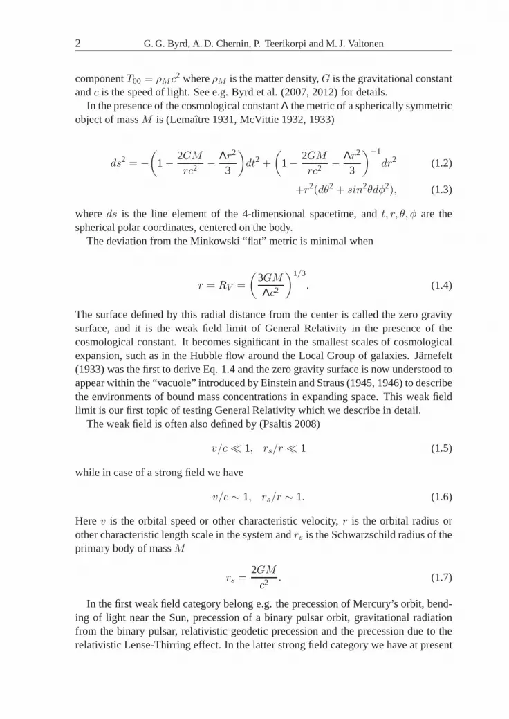
day in 2007 September (UT)

’OJdaily_flux’’05theory’

Figure 7. The optical light curve of OJ287 during the 2007 September outburst. Onlylow polarization (less than 10%) data points are shown. The dashed line is the theoreticalfit. The arrow points to September 13.0, the predicted time oforigin of the rapid fluxrise.

Lehto and Valtonen (1996) found a solution from five flares which already proved thecase in the first approximation.

At a deeper level one has to consider the astrophysical processes that generate theflares. The flares start very suddenly, with the rise time of only about one day (Figure7). This fact alone excludes many possibilities that one might be otherwise tempted toconsider: Doppler boosting variation from a turning jet or increased accretion rate dueto varying tidal force. The timescales associated with these processes are months toyears quite independent of a detailed model. It turns out that the base level of emissionof OJ287, which is synchrotron radiation from the jet, is affected by both of thesemechanisms. The Doppler boosting variation accounts for the 55 year cycle (Valtonenand Pihajoki 2013) while the varying tides change the base level in a 11.8 year cycle(Sundelius et al. 1997). Also the∼ 50 day cyclic component is due to tides (Figure8), but via a density wave at the innermost stable orbit of theprimary accretion disk(Pihajoki et al. 2013).

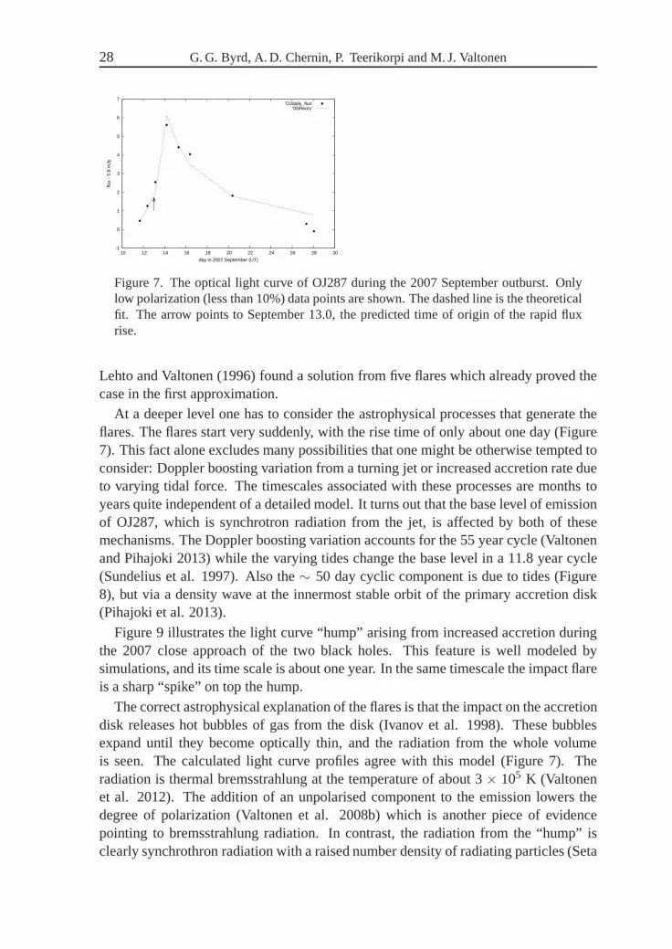
Figure 9 illustrates the light curve “hump” arising from increased accretion duringthe 2007 close approach of the two black holes. This feature is well modeled bysimulations, and its time scale is about one year. In the sametimescale the impact flareis a sharp “spike” on top the hump.

The correct astrophysical explanation of the flares is that the impact on the accretiondisk releases hot bubbles of gas from the disk (Ivanov et al. 1998). These bubblesexpand until they become optically thin, and the radiation from the whole volumeis seen. The calculated light curve profiles agree with this model (Figure 7). Theradiation is thermal bremsstrahlung at the temperature of about 3× 105 K (Valtonenet al. 2012). The addition of an unpolarised component to theemission lowers thedegree of polarization (Valtonen et al. 2008b) which is another piece of evidencepointing to bremsstrahlung radiation. In contrast, the radiation from the “hump” isclearly synchrothron radiation with a raised number density of radiating particles (Seta


1

2

3

4

5

6

7

300 400 500 600 700 800 900

mJy

Day

period 51.5 d

rms error 0.57 mJy

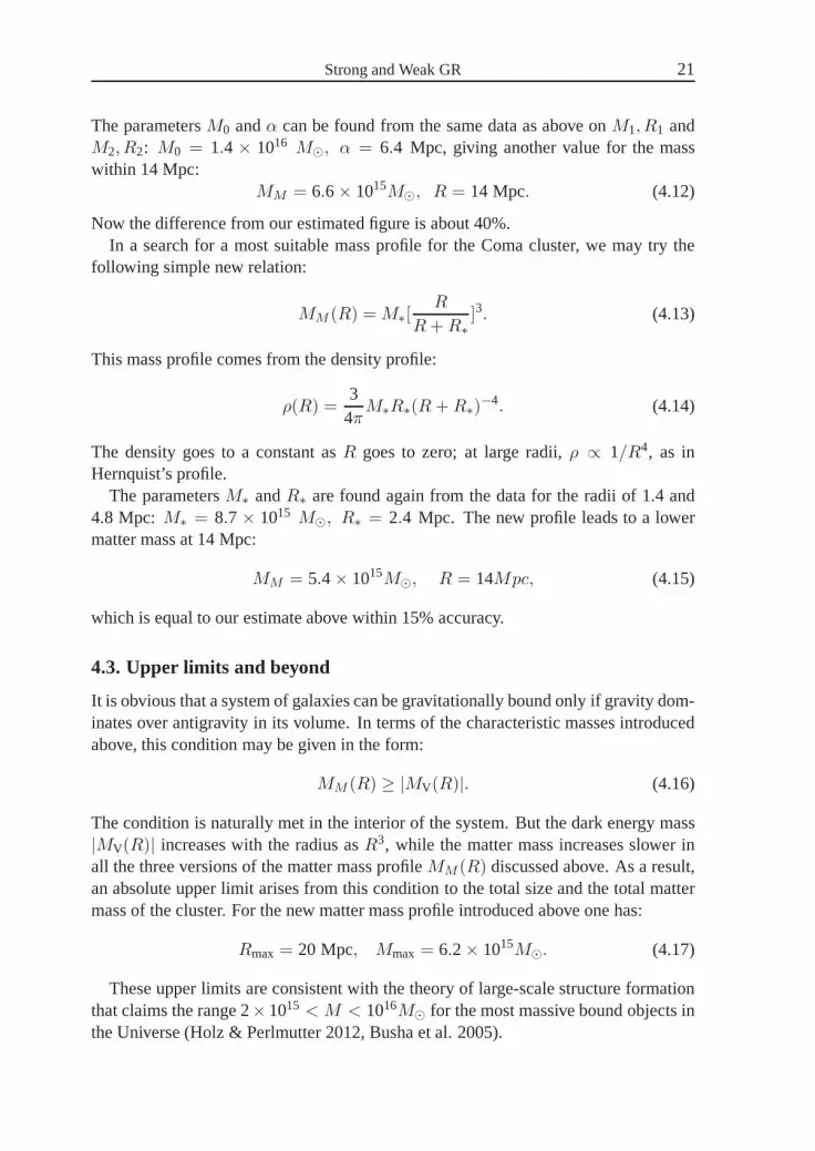
amplitude 1.14 mJyOJ287 2004-2006

Figure 8. The optical light curve of OJ287 during 2004-2006,using 10 day averages(squares). The 2005 impact flare is excluded. The three starsare points which are notused in the periodicity fit. The best fit for the remaing data isa 51.5 day period. Ifinterpreted as the half-period of the innermost stable orbit, this impliesχ1 = 0.25.

0

2

4

6

8

10

12

2006 2006.5 2007 2007.5 2008 2008.5

V-f

lux,

mJy

time, yr

low polarization flux in OJ287

Figure 9. The optical light curve of OJ287 during 2006-2008.Only low polarization(less than 10%) data points are shown.


et al. 2009). OJ287 is the only quasar which is known to have bremsstrahlung flares,and as such these flares give a unique set of signals to be used in orbit determination.

What is more important, the model is able to predict future outbursts. The predictionfor the latest outburst was 2007 September 13 (Valtonen 2007, 2008a), accurate to oneday, leaving little doubt about the capability of the model (see Figure 7; the predictedtime refers in this case to the start of the rapid flux rise.) The 2007 September 13outburst was an observational challenge, as the source was visible only for a shortperiod of time in the morning sky just before the sunrise. Therefore a coordinatedeffort was made starting with observations in Japan, then moving to China, and finallyto central and western Europe. The campaign was a success andfinally proved thecase for the binary model (Valtonen et al. 2008b).

We see from Figure 7 that the observed flux rise coincides within 6 hours with theexpected time. The accuracy is about the same with which we were able to predict thereturn of Halley’s comet in 1986!

The astrophysical model introduces a new unknown parameter, the thickness of theaccretion disk. For a given accretion rate which is determined from the brightness ofthe quasar (considering the likely Doppler boosting factor), the thickness is a functionof viscosity in the standardα disk theory of Shakura and Sunyaev (1973) and in itsextension to magnetic disks by Sakimoto and Corotini (1981). The value of the vis-cosity coefficientα ∼ 0.3 is rather typical for other accreting systems (King et al.2007). Different values ofα lead to different delay times between the disk impactand the optical flare. The delay can be calculated exactly except for a constant factor;this factor is an extra parameter in the model. The problem remains mathematicallywell defined. In fact, using only 6 outbursts as fixed points inthe orbit, it is possibleto solve the four orbital parameters plus the time delay parameter (in effectα) in thefirst approximation (Valtonen 2007). The success of this model in predicting the 2007outburst was encouraging.

The future optical light curve of OJ287 was predicted from 1996 to 2030 by Sun-delius et al. (1997); they published the expected optical flux of OJ287 for everytwo-week interval between 1900 and 2030. During the first fifteen years OJ287 hasfollowed the prediction with amazing accuracy, producing five outbursts at expectedtimes, of expected light curve profile and size. It is extremely unlikely that such acoincidence should have happened by chance: these optical flux variations alone haveexcluded alternative models such as quasiperiodic oscillations in an accretion disk atthe 5σ confidence level (Valtonen et al. 2011b).

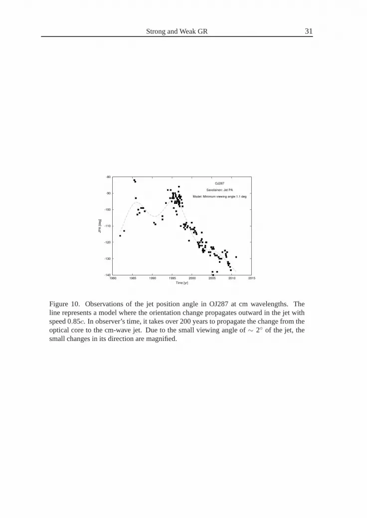
OJ287 is unresolved in optical, but in radio and X-ray wavelengths we observe along jet. The radio jet has been observed since early 1980’s and its orientation showsinteresting, but in no way simple 12 year cycles. In Figure 10we show the positionangle (PA) observations of the jet as a function of time (Valtonen and Wiik 2012). Theline follows a model where the binary shakes the accretion disk gravitationally. Thisshaking is transmitted to the jet. With suitably chosen parameters the binary actionexplains not only the cm-wave observations of Figure 10, butalso quite different mm-


Figure 10. Observations of the jet position angle in OJ287 atcm wavelengths. Theline represents a model where the orientation change propagates outward in the jet withspeed 0.85c. In observer’s time, it takes over 200 years to propagate thechange from theoptical core to the cm-wave jet. Due to the small viewing angle of∼ 2 of the jet, thesmall changes in its direction are magnified.


wave jet wobble, in addition to the changes in the optical polarization angle (Valtonenand Pihajoki 2013). All these phenomena occur in the jet, farfrom the primary sitesof action, and thus they cannot be used for high precision determination of the orbit.

The orbital parameters may be determined from the basic binary model withoutfurther knowledge of the orbit solution. The precession rate may be estimated bytaking the ratio of the two dominant variability frequencies in the optical light curve,averaged over one month to minimize the effects of the impactflares on the analysis. Ifone of the frequencies (11.8 yr) relates to the orbital period while the other frequency(55 yr) arises from precession (Valtonen et al. 2006), then their ratio will tell whatfraction of the angleπ the major axis of the orbit precesses per period. Due to thesymmetry of the accretion disk relative to its midplane, theprecessional effects shouldrepeat themselves after rotation by 180. Therefore the precession rate per orbitalperiod should be 11.8× 180/55= 38.6. Once the precession rate is known, we get agood first estimate for the mass of the primarym1 ∼ 1.8 · 1010M⊙.

The secondary mass was determined by Lehto and Valtonen (1996), m2 = 1.44 ·108M⊙, when adjusted to the ’current’ Hubble constant of 70 km/s/Mpc and to the5.6 mJy outburst strength, as observed in 2007. The mass value is based on the as-trophysics of the impact and the strength of the maximum signal (Ivanov et al. 1998,Valtonen et al. 2012). A large mass ratio is necessary for thestability of the accretiondisk. The primary black hole needs to be at least∼ 130 times more massive than thesecondary (Valtonen et al. 2012). The values ofm1 andm2 satisfy this requirement.

The moderately high eccentricitye ∼ 0.7 is expected at a certain stage of inspiralof binary black holes of large mass ratio (Baumgardt et al. 2006, Matsubayashi etal. 2007, Iwasawa et al. 2011). Dynamical interaction with the stars of the galacticnucleus drives the eccentricity toe ∼ 0.99 before the gravitational radiation takes overin the evolution of the binary major axis. When the binary is at the evolutionary stagewhere OJ287 is now, the eccentricity has dropped toe ∼ 0.7.

The value ofχ1 may be determined from the period of the innermost stable orbit.The best determination for this period is 103± 4 days which corresponds toχ1 =0.25± 0.04.

The first two columns of Table 5 summarize the parameters determined by astro-physics of the binary black hole system. No information on the outburst timing hasbeen used in the astrophysical model.

8 Modeling with Post Newtonian methods

The Post Newtonian approximation to General Relativity provides the equations ofmotion of a compact binary as corrections to the Newtonian equations of motion inpowers of(v/c)2 ∼ GM/(c2r), wherev, M , andr are the characteristic orbital ve-locity, the total mass, and the typical orbital separation of the binary, respectively. Theapproximation may be extended to different orders. The terminology 2PN, for exam-ple, refers to corrections to Newtonian dynamics in powers of (v/c)4. Valtonen et al.


(2010a) use the 2.5PN and Valtonen et al. (2011a) 3PN-accurate orbital dynamics thatincludes the leading order general relativistic, classical spin-orbit and radiation reac-tion effects for describing the evolution of a binary black hole (Kidder 1995). Thefollowing differential equations describe the relative acceleration of the binary and theprecessional motion for the spin of the primary black hole at2.5PN order:

x ≡ d2x

dt2= x0 + x1PN + xSO + xQ

+x2PN + x2.5PN , (8.1)

ds1

dt= ΩSO × s1 , (8.2)

wherex = x1 − x2 stands for the center-of-mass relative separation vector betweenthe black holes with massesm1 andm2 andx0 represents the Newtonian accelerationgiven by

x0 = −Gm

r3 x , (8.3)

m = m1 + m2 andr = |x|. Kerr parameterχ1 and the unit vectors1 define thespin of the primary black hole by the relationS1 = Gm2

1 χ1 s1/c andχ1 is allowed totake values between 0 and 1 in general relativity.ΩSO provides the spin precessionalfrequency due to spin-orbit coupling. The PN contributionsoccurring at the conser-vative 1PN, 2PN and the reactive 2.5PN orders, denoted by ¨x1PN , x2PN andx2.5PN ,respectively, are non-spin by nature. The explicit expressions for these contributions,suitable for describing the binary black hole dynamics, are(Mora and Will 2004)

x1PN = −Gmc2 r2

n[

−2(2+ η)Gmr (8.4)

+(1+ 3η)v2 − 32ηr

2]

− 2(2− η)rv

,

x2PN = −Gmc4 r2

n

[

34(12+ 29η)

(

Gmr

)2(8.5)

+η(3− 4η)v4 + 158 η(1− 3η)r4

−32η(3− 4η)v2r2 − 1

2η(13− 4η)(Gmr ) v2 (8.6)

−(2+ 25η + 2η2)(Gmr ) r2

]

−12rv

[

η(15+ 4η)v2 − (4+ 41η + 8η2)(Gmr )

−3η(3+ 2η)r2]

,


(8.7)

x2.5PN = 815

G2m2ηc5r3

[

9v2 + 17Gmr

]

rn (8.8)

−[

3v2 + 9Gmr

]

v

,

where the vectors ˆn andv are defined to be ˆn ≡ x/r andv ≡ dx/dt, respectively,while r ≡ dr/dt = n · v, v ≡ |v| and the symmetric mass ratioη = m1 m2/m

2.The leading order spin-orbit contributions to ¨x, appearing at 1.5PN order (Barker

and O’Connell 1975a), read

xSO = Gmr2

(

Gmc3 r

)

(

1+√

1−4η4

)

(8.9)

χ1

[

12 [s1 · (n× v)]

]

n

+

[

(

9+ 3√

1− 4η)

r

]

(n× s1)

−[

7+√

1− 4η

]

(v × s1)

,

while

ΩSO =

(

Gmη

2c2 r2

)(

7+√

1− 4η

1+√

1− 4η

)

(n× v) . (8.10)

(8.11)

Finally, the quadrupole-monopole interaction term ¨xQ, entering at the 2PN order(Barker and O’Connell 1975a), reads

xQ = −q χ21

3G3 m21m

2c4 r4

[

5(n · s1)2 − 1

]

n

−2(n · s1)s1

, (8.12)

where the parameterq, whose value is 1 in general relativity, is introduced to test theblack hole ‘no-hair’ theorems (Will 2008).

It turns out that adding the 3PN contributions tod2x/dt2, are not necessary; their

influence falls within error limits of the OJ287 problem. It has been important to verifythat the PN series converges rapidly enough to ingore the terms of order higher than2.5PN. Similarly, the terms related to the spin of the secondary turn out be negligle in


-10

-8

-6

-4

-2

0

2

4

6

0 200 400 600 800 1000 1200

degr

ees

years

Sx

Sy

Ω /100

Figure 11. The circulation of the ascending node (Ω) of the orbit (straight line) in thecoordinate system in which the initial spin vectors1 points to the direction of the z-axis.The quantities plotted areΩ/100 in degrees and the symbolssx andsy correspond to thex andy components of the spin-direction vectors1 in degrees..

the OJ287 problem (Valtonen et al. 2011a). The precessionalmotion for the spin ofthe primary black hole is 2PN accurate in our calculations.

The main consequence of including the leading order spin-orbit interactions to thedynamics of a binary black hole is that it forces the orbital plane to precess. The orbitalangular momentum vector, characterising the orbital plane, precesses around the spinof the primary in such a way that the angle between the orbitalplane and the spin vectors1 remains almost constant (roughly within±0.5 in the model). The spin-vector itselfprecesses drawing a cone with an opening angle of about 8 degrees (see Figure 11).

The precessional period for both the orbital plane and the spin of the binary, pro-vided by|ΩSO|, is about 1300 years for the orbital parameters of OJ287. Thepreces-sion cone axis coincides with the mean accretion disk axis. It is reasonable to expectsuch a situation due to the Bardeen-Petterson effect (Kumarand Pringle 1985). Be-cause the time scale of the Bardeen-Petterson effect is muchlonger than the black holespin precession time scale (Lodato and Pringle 2006), the disk axis is not able to followthe rapid precession of the primary spin axis.

The orbit solutions currently involvenine accurately timed outbursts as listed inTable 6. The orbit solutions provide a unique set of parameters (Table 5, column 3).Recently also the tenth outburst from 1906 has been added (Hudec et al. 2013). In thiscase there are only limits for the timing; the main influence of including the 1906 datais to bringχ1 to ∼ 0.23, somewhat below the range given in Table 5. Note that theeccenticitye is defined as

rarp

=1+ e

1− e, (8.13)

wherera andrp are the apocenter and pericenter distances in the orbit, respectively.


The instantaneous eccentricity varies during a relativistic binary orbit; in this way weget a definite number that resembles the eccentricity of a Keplerian orbit.

Because we are using 8 time intervals to fit 8 parameters, the fit has no degrees offreedom. The tolerance limits of Table 5 are a consequence ofhaving a tolerance inthe fixed points of the outburst times (Table 6). The no-hair parameterq is the eigthparameter which of course should beq = 1 if General Relativity is correct.

As part of the solution we obtain the list of all past and future outburst times withtheir uncertainties. For example, the well recognized outbursts in 1959, 1971 and 1994are timed at 1959.213±0.002, 1971.1265±0.002 and 1994.6085±0.005, respectively.In all these cases data are missing at the crucial time of expected rapid flux rise, andthus these predictions cannot be verified at present.

It is remarkable that the two sets of parameters in second andthird columns ofTable 1 agree so closely. If the basic model were not correct,there would be no reasonfor this agreement. Also, the mere fact that an orbit solution exists at all is a strongargument for the model.

Let us now turn our attention to the expected future outbursts in OJ287. We expectthree more outbursts during the next two decades, occuring in 2016, 2019 and 2022.The 2016 outburst should be an easy one to detect, as it comes in January of that year.Its timing is spin-sensitive; the exact date will give us a good spin value from thefollowing formula:

χ1 = 0.25− 0.5× (t− 2016.0). (8.14)

Heret is the time of the beginning of the outburst in years. The expected accuracyis 0.005 units inχ1. The dependence onq is secondary, and thus the 2016 outbursttiming is of no use by itself for the testing of the no-hair theorem.

The value ofq is currently best determined by the 1995 outburst. There wasanintensive monitoring campaign of OJ287 (called OJ94) during this outburst season, butunfortunately there exists a gap in these observations justat the crucial time (Valtonen1996, Figure 12). It may still be possible that there are measurements somewherewhich are not recorded in the OJ94 campaign light curve, and which would be valuablein narrowing downq even from these data. The line in Figure 12 is drawn using thewell observed 2007 outburst as a template to compare with 1995. It is should be notedthat even a few more measurements of 1995 could narrow down the range ofq.

The 2019 outburst timing is also sensitive to theq:

q = 1.0− 1.2× (t− t0), (8.15)

wheret is time of the beginning of the outburst (in days) andt0 is 2019 July 14,11:19 UT. The expected accuracy for theq determination is 0.15 units, i.e. optimallythe accuracy of the no-hair theorem test is doubled in comparison with the presentuncertainty. Observing OJ287 during the rising flux of the 2019 outburst, from July14 to July 17, is a challenge for ground based observers. Thisis because the angular


-0.5

0

0.5

1

1.5

2

-1 -0.5 0 0.5 1 1.5 2

Vflu

x -

2.18

Day - Julian Day 2450026.65

Beginning of the 1995 outburstat 1995.843

Figure 12. The observations of OJ287 during 4 - 7 November 1995, transformed tooptical V-band. Overlaid is the theoretical light curve profile, corresponding toq = 1.The zero point of the time axis is at 3:36 UT of 1995, November 5. The peak flux of 5.1mJy above the base level was predicted for November 8 (Lehto and Valtonen 1996), butthere were no observations to confirm it. The data on November9 and later suggest thatthe outburst maximum was probably missed.

distance between the Sun and OJ287 is only about 19 degrees atthe beginning ofthe event, and goes down to about 16 degrees by the time of the peak flux on July17. T. Pursimo has measured OJ287 at the Nordic Optical telescope on 2007 July 12(Valtonen et al. 2009) which demonstrates that the July measurements should alsobe feasible in 2019. Space observations would also be usefulin order to study theoutburst over a wider spectral range. The 2022 outburst is scheduled practically atthe same time of year as the 2019 outburst. Obviously it wouldalso be of interestto observe this event as it would tie down the parameters of the general model morenarrowly. However, it will not give any further informationon q.

9 OJ287 results at the strong field limit

The binary black hole in OJ287 is modeled to contain a spinning primary black holewith an accretion disk and a spinning or non-spinning secondary black hole. UsingPN-accurate dynamics, relevant for such a system, we infer that the primary blackhole should spin approximately at one quarter of the maximumspin rate allowed ingeneral relativity. In addition, the ‘no-hair theorems’ ofblack holes (Misner et al.1973) are supported by the model, although the testing is possible only to a limitedprecision. The solutions concentrate aroundq = 1.0 with one standard deviation of0.3 units. These results are achieved with the help of new data on historical outburstsas well as using the most recent outburst light curves together with the timing modelfor OJ287 outbursts (Valtonen et al. 2007).

Further, a polar orbit is assumed. Any other high inclination model would give us


the same timing results. Sundelius et al. (1997) carried outsimulations with a numberof different inclinations between the disk and the orbit, and found that the inclinationmakes no difference. This is not surprising since the impacts occur along the line ofnodes, and the timing of the impacts is not a function of the impact angle. We havetried varying the spin angle relative to the disk, and found that within reasonable limits(we considered inclinations up to 10) the results do not change. Again this is whatis expected since the line of nodes circulates slowly in comparison with the orbitalangular motion.

The reason why we would expect at least approximate alignment between the blackhole spin and the disk spin is the Bardeen - Petterson effect which tends to align thetwo spins. However, the alignment time scale is much slower (about 107 yr, Lodato& Pringle 2006) than the spin precession time, and thus the disk does not follow theblack hole spin exactly but only on average.

In this scenario, we have a unique solution and also a unique prediction for the nextOJ287 outburst, expected in 2016. We should then be able to judge the correctnessof the present solution. Note that an outburst is not expected in 2016 in any simpleextrapolation from past observations, as it is well before the average 12 yr cycle isdue, and thus it is a sensitive test of the general model as well as a test for the spin ofthe primary black hole. The observations of the 2019 outburst will then improve theaccuracy of the ’no-hair’ theorem test by a factor of two, to the level of 15%.

There are at least 5 additional outbursts in the historical record which have not yetbeen been accurately observed. If new data of these outbursts are found it will openup the possibility of improving the model and improving thataccuracy of the no-hairtheorem test to the level of 10%. Searches of plate archives are recommended for thispurpose.

10 Summary and Conclusions on General Relativity at weakand strong field limits

We have discussed the amazing range of validity of General Relativity from tests fromthe weak to strong field limits. The weak field corresponds to speeds much less thanthat of light or distances much larger than the Schwarzschild radius of the primary bodyof an orbiting pair. In weak field tests, we briefly reviewed the precession of Mercury’sorbit, bending of light near the Sun, precession of a binary pulsar orbit, gravitationalradiation from the binary pulsar, relativistic geodetic precession and the precession dueto the relativistic Lense-Thirring effect. In all these cases General Relativity accountsfor the observations but, the cosmological constant (manifested as dark energy) is notsignificant.

However, the existence of dark energy in General Relativitycan be tested in theweak field limit. Einstein (1917) proposed a cosmological constant specified to pro-duce a static universe. Evolving models of the universe werederived by Alexander


Friedmann (1922, 1924) and Georges Lemaitre (1927). The Einstein static solutionis a special case, where the cosmological constant is related to the matter density togive gravity-antigravity balance. In general there are no theoretical restrictions on thecosmological constant. The universe expands or contracts as a whole. The Hubble dis-covery of the redshift distance relation (Hubble 1929) can be regarded as a predictiveverification of General Relativity.

After the discovery of the Big Bang, it seemed that the cosmological constant couldnot be as big as Einstein required for a static universe. It was subsequently commonlyassumed to be zero. However, when supernovae of type Ia were used to estimatedistances of galaxies whose redshiftsz ∼ 1, a positive cosmological constant wasindicated (Riess et al. 1998 and Perlmutter et al. 1999).

We describe in detail how to test the existence of dark energyat the weak field limitof General Relativity via an outflow model in groups and clusters of galaxies (Chernin2001; Chernin et al. 2006; Byrd et al. 2011). The Local Group has been found to haveoutflowing dwarf galaxies around it (van den Bergh 1999; Karachentsev et al. 2009).The dwarfs’ motion indicates not only the gravitational mass of the group but also thedark energy background (Chernin et al. 2009). Studies the Virgo and Fornax clustersand even rich clusters like Coma (Karachentsev et al. 2003, Chernin 2008, Chernin etal. 2006, 2007, 2010, 2012a,b, Chernin 2013) show similar structure.

There has been been a large amount of effort to determine the value of the cosmolog-ical constant, and its possible dependence on redshift or, equivalently, time (Friemanet al. 2008, Blanchard 2010, Weinberg et al. 2013). In the literature from year 2005onwards, values cluster aroundΩΛ = 0.73 with a standard deviation of 0.044, the typi-cal error in individual measurements. Only the cosmic microwave background (CMB)models give a significantly better accuracy, but even in thiscase one may suspect hid-den systematic errors due to foreground corrections (Whitbourn et al. 2014). In ouranalysis of the literature including nearby groups and clusters, within the error limits,Λ appears to be a constant over the redshift range from cosmological to Local Groupoutflows, an impressive validation.

The strong field corresponds to speeds comparable to that of light or distances com-parable to the Schwarzschild radius of the primary body of a pair. An important strongfield test is to be sure that black holes are indeed the singularities predicted in GeneralRelativity. We have to ascertain that at least in one case thespacetime around a sus-pected black hole satisfies the no-hair theorems which statethat an electrically neutralrotating black hole in General Relativity is completely described by its mass,M , andits angular momentum,S, implying that the multipole moments, required to specifythe external metric are fully expressible in terms ofM andS. No-hair theorems applyonly in General Relativity, and thus are a powerful eliminator of various alternativetheories of gravitation (Will 2006, Yunes and Siemens 2013,Gair et al. 2013).

An ideal test of the no-hair theorem is to have a test particlein orbit around a spin-ning black hole. We have described results for one such system, the BL Lacertae objectOJ287, a binary black hole of very large mass ratio. OJ287 gives outbursts during the


secondary’s periodic orbital disk crossings of an accretion disk around the more mas-sive member. The timing of the repeating outbursts gives theorbit and the primary’squadrupole parameter. Post-Newtonian dynamics, necessary for such a system, im-plies that the primary black hole should spin at about one quarter of the maximum spinrate allowed in General Relativity. The ’no-hair theorems’of black holes (Misner etal. 1973) are supported by the model but with a limited precision at present (Valtonenet al. 2011a). Observations of predicted 2016 and 2019 outbursts and collection ofdata on more past outbursts should improve the accuracy of the ’no-hair’ theorem test.This extreme test at the strong field limit supports General Relativity.

Acknowledgments. We note that Bruce Barker (who died in 1988 at the age of 54)was a co-author of two important theoretical papers testingGeneral Relativity in ex-treme binary systems like those discussed here. He was a friend and colleague of M.V. and G. B. at the University of Alabama.

Bibliography

[1] A. Einstein, Die Grundlage der allgemeinen Relativitätstheorie,Annalen der Physik, 354(1916), 769–822.

[2] A. Einstein, Kosmologische Betrachtungen zur allgemeinen Relativitätstheorie,Sitzungs-berichte der Königlich Preussischen Akademie der Wissenschaften (Berlin), (1917), 142–152.

[3] G.G. Byrd, A.D. Chernin and M.J. Valtonen,Cosmology: Foundations and Frontiers,Moscow, URSS (2007).

[4] G. Byrd, A. D. Chernin, P. Teerikorpi and M. Valtonen,Paths to Dark Energy, De Gruyter,(2012).

[5] G. Lemaître, The expanding universe,Monthly Notices of the Royal Astronomical Society,91 (1931), 490–501.

[6] G.C. McVittie, Condensations in an expanding universe,Monthly Notices of the RoyalAstronomical Society, 92 (1932), 500–518.

[7] G.C. McVittie, The mass-particle in an expanding universe,Monthly Notices of the RoyalAstronomical Society, 93 (1933), 325–339.

[8] G. Järnefelt, Über die Bewegung eines Massenpunktes in einem Raum mit zentralsym-metrischer Massen- und Druckverteilung,Zeitschrift für Astrophysik, 7 (1933), 326–327.

[9] A. Einstein and E. G. Straus, The Influence of the Expansion of Space on the GravitationFields Surrounding the Individual Stars,Reviews of Modern Physics, 17 (1945), 120–124.

[10] A. Einstein and E.G. Straus, Corrections and Additional Remarks to our Paper: TheInfluence of the Expansion of Space on the Gravitation FieldsSurrounding the IndividualStars,Reviews of Modern Physics, 18 (1946), 148–149.

[11] D. Psaltis, Probes and Tests of Strong-Field Gravity with Observations in the Electro-magnetic Spectrum,Living Reviews in Relativity, 11 (2008), 9:1–9:61.


[12] U. Le Verrier, Lettre de M. Le Verrier à M. Faye sur la theorie de Mercure et sur lemouvement du perihelie de cette planeteComptes rendus hebdomadaires des seances del’Academie des sciences (Paris), 49 (1859), 379–383.

[13] S. Newcomb,The elements of the four inner planets and the fundamental constants,(Washington, D. C., U. S. Govt. Office, 1895).

[14] A. Hall, A suggestion in the theory of Mercury,Astron. J., 14 (1894), 49–51.

[15] I. I. Shapiro, C. C. Counselman III and R. W. King, Verification of the principle of equiv-alence for massive bodies,Phys. Rev. Lett., 36 (1976), 555–558.

[16] A. Einstein, Erklärung der Perihelbewegung des Merkuraus der allgemeinen Relativität-stheorieSitz. Preuss. Akad. Wiss., 11 (1915), 831–839.

[17] R. A. Hulse and J. H. Taylor, Discovery of a pulsar in a binary system,Astrophys. J., 195(1975), L51–L53.

[18] J. H. Taylor and J. M. Weisberg, Further experimental tests of relativistic gravity usingthe binary pulsar PSR 1913 + 16,Astrophys. J., 345(1989), 434–450.

[19] T. Damour and J. H. Taylor, On the orbital period change of the binary pulsarPSR1913+16,Astrophys. J., 366(1991), 501–511.

[20] R. A. Hulse, The discovery of the binary pulsar,Rev. Mod. Phys., 66 (1994), 699–710.

[21] A. G. Lyne et al., A Double–Pulsar System: A Rare Laboratory for Relativistic Gravityand Plasma Physics,Science, 303(2004), 1153–1157.

[22] M. Kramer et al., Tests of General Relativity from Timing the Double Pulsar,Science,314(2006), 97–102.

[23] J. Lense and H. Thirring, Über den Einfluss der Eigenrotation der Zentralkörper aufdie Bewegung der Planeten und Monde nach der Einsteinschen Gravitationstheorie.Physikalische Zeitschrift, 19 (1918), 156–163.

[24] I. Cuifolini and E. C. Pavlis, A confirmation of the general relativistic prediction of theLense-Thirring effect,Nature, 431(2004), 958–960.

[25] C. W. F. Everitt et al., Gravity Probe B: Final Results ofa Space Experiment to TestGeneral Relativity,Physical Review Letters, 106(2011), 221101-1–221101-5

[26] T. Damour and R. Ruffini, Certain new verifications of general relativity made possible bythe discovery of a pulsar belonging to a binary system,Acad. Sci. Paris Comptes RendusSer. Sci. Math., 279(1974), 971–973.

[27] B. M. Barker and R. F. O’Connell, Gravitational two-body problem with arbitrary masses,spins, and quadrupole moments,Physical Review D, 12 (1975a), 329–335.

[28] B. M. Barker and R. F. O’Connell, Relativistic effects in the binary pulsar PSR 1913+16,Astrophys.J.Lett., 199(1975b), L25–L26.

[29] J. M. Weisberg and J. H. Taylor, 2005, The Relativistic Binary Pulsar B1913+16: ThirtyYears of Observations and Analysis,Binary Radio Pulsar, ASP Conference Series, Editors:F. A. Rasio and I. H. Stairs, 328(2005), 25–31.


[30] J. M. Weisberg, D. J. Nice and J. H. Taylor, 2010, âAIJTiming Measurements of theRelativistic Binary Pulsar B1913+16 âAI Astrophys.J., 722(2010), 1030–1034.

[31] A. Einstein, Über den Einfluss der Schwerkraft auf die Ausbreitung des LichtesAnnalender Physik, 340(1911), 898–908.

[32] A. S. Eddington, The total eclipse of May 29 and the influence of gravitation on light,Observatory, 42 (1919), 119–122.

[33] F. W. Dyson, A. S. Eddington and C. R. Davidson, C., A Determination of the Deflectionof Light by the Sun’s Gravitational Field, from Observations Made at the Total Eclipseof May 29, 1919,Philosophical Transactions of the Royal Society of London.Series A,Containing Papers of a Mathematical or Physical Character, 220(1920), 291–333.

[34] D. Walsh, R. F. Carswell and R. J. Weymann, 0957 + 561 A, B âAS twin quasistellarobjects or gravitational lens,Nature, 279(1979), 381-384.

[35] M. J. Valtonen and H. J. Lehto, Outbursts in OJ 287: A New Test for the General Theoryof Relativity,Astrophysical Journal Letters, 481(1997), L5–L7.

[36] Y.-T. Sun, J.-Y. Liu, J.-Z. Liu, Y.-L. Ai, M. Zhou and E.-L. Qiao, A Research on theGravitational Wave Radiation of OJ 287,Chinese Astronomy and Astrophysics, Volume35 (2011), 123–132.

[37] J. Liu, Y. Zhang, H. Zhang, Y. Sun and N. Wang, Determining gravitational wave radia-tion from close galaxy pairs using a binary population synthesis approach,Astronomy andAstrophysics, Volume540(2012), A67:1–A67:6.

[38] R. P. Kerr, Gravitational Field of a Spinning Mass as an Example of Algebraically SpecialMetrics,Physical Review Letters, 11 (1963), 237–238.

[39] M. J. Valtonen et al., Measuring black hole spin in OJ287, Celestial Mech. and DynamicalAstr., 106(2010b), 235–243.

[40] W. Israel, Event horizons in static vacuum spacetimes,Phys.Rev.164(1967), 1776–1779.

[41] W. Israel, Event horizons in static electrovac spacetimes,Commun. Math.Phys.8 (1968),245–260.

[42] B. Carter, An axisymmetric black hole has only two degrees of freedom,Phys.Rev.Lett.26 (1970), 331–333.

[43] S. W. Hawking, Gravitational radiation from collidingblack holes,Phys.Rev.Lett.26(1971), 1344–1346.

[44] S. W. Hawking, Black holes in general relativity,Commun.Math.Phys.25 (1972), 152–166.

[45] C. W. Misner, K. S. Thorne and J. A. Wheeler,Gravitation(W.H.Freeman & Sons, SanFrancisco, p. 876, 1973).

[46] A. A. Friedmann, Über die Krümmung des Raumes,Zeitschrift für Physik, 10 (1922),377–386.

[47] A. A. Friedmann, Über die Möglichkeit einer Welt mit konstanter negativer Krümmungdes Raumes,Zeitschrift für Physik, 21, 326–332.


[48] G. Lemaitre, Un Univers homogene de masse constante et de rayon croissant rendantcompte de la vitesse radiale des nebuleuses extra-galactiques,Annales de la Societe Sci-entifique de Bruxelles, A47 (1927), 49–59.

[49] E. Hubble, A Relation between Distance and Radial Velocity among Extra-Galactic Neb-ulae,Proceedings of the National Academy of Sciences of the United States of America,15 (1929), 168–173.

[50] A. G. Riess et al., Observational evidence from supernovae for an accelerating universeand a cosmological constant,Astron. J., 116(1998) 1009–1038.

[51] S. Perlmutter et al., Measurements of Omega and Lambda from 42 High-Redshift Super-novae,Astrophys. J., 517(1999), 565–586.

[52] A.D. Chernin, Reviews of topical problems: Cosmic vacuum, Physics Uspekhi, 44(2001), 1099–1118.

[53] A.D. Chernin, P. Teerikorpi and Yu.V. Baryshev, Non-Friedmann cosmology for the Lo-cal Universe, significance of the universal Hubble constant, and short-distance indicatorsof dark energy,Astronomy and Astrophysics, 456(2006), 13–21.

[54] S. van den Bergh, The local group of galaxies,Astronomy and Astrophysics Review, 9(1999), 273–318.

[55] I. D. Karachentsev, O. G. Kashibadze, D. I. Makarov and R. B. Tully, The Hubble flowaround the Local Group,Monthly Notices of the Royal Astronomical Society, 393(2009),1265–1274.

[56] A.D. Chernin et al., Local dark matter and dark energy asestimated on a scale of 1 Mpcin a self-consistent way,Astronomy and Astrophysics, 507(2009), 1271–1276.

[57] Yu.V. Baryshev, A.D. Chernin and P. Teerikorpi, The cold local Hubble flow as a signa-ture of dark energy,Astronomy and Astrophysics, 378(2001), 729–734.

[58] P. Teerikorpi, A.D. Chernin and Yu.V. Baryshev, The quiescent Hubble flow, local darkenergy tests, and pairwise velocity dispersion in aΩ = 1 universe,Astronomy and Astro-physics, 440(2005), 791–797.

[59] I.D. Karachentsev et al., Local galaxy flows within 5 Mpc, Astronomy and Astrophysics,398(2003), 479–491.

[60] P. Teerikorpi, A.D. Chernin, I.D. Karachentsev and M.J. Valtonen, Dark energy in theenvironments of the Local Group, the M 81 group, and the CenA group: the normalizedHubble diagram,Astronomy and Astrophysics, 483(2008), 383–387.

[61] A.D. Chernin et al., The very local Hubble flow: Computersimulations of dynamicalhistory,Astronomy and Astrophysics, 415(2004), 19–25.

[62] S. Peirani and J.A. de Freitas Pacheco, Dynamics of nearby groups of galaxies: the roleof the cosmological constant,Astronomy and Astrophysics, 488(2008), 845–851.

[63] J. Saarinen and P. Teerikorpi,arXiv: 1402.0950(2013).

[64] M.J. Valtonen, G.G. Byrd, M.L. McCall and K.A. Innanen,A revised history of the LocalGroup and a generalized method of timing,Astronomical Journal, 105(1993), 886–893.


[65] G. Byrd, M. Valtonen, M. McCall and K. Innanen, Orbits ofthe Magellanic Clouds andLeo I in local group history,Astronomical Journal, 107(1994), 2055–2059.

[66] A.D. Chernin et al., Local dark energy: HST evidence from the vicinity of the M81/M82galaxy group,Astrophysics, 50 (2007), 405–415.

[67] P. Teerikorpi and A.D. Chernin, The Hubble diagram for asystem within dark energy: thelocation of the zero-gravity radius and the global Hubble rate,Astronomy and Astrophysics,516(2010), A93:1–A93:4.

[68] F.D. Kahn and L. Woltjer, Intergalactic Matter and the Galaxy, Astrophysical Journal,130(1959), 705–717.

[69] J. Binney and S. Tremaine,Galactic Dynamics: Second Edition, Princeton UniversityPress, Princeton, NJ USA, (2008).

[70] S. Garrison-Kimmel, M. Boylan-Kolchin, J. Bullock andK. Lee, ELVIS: Exploring theLocal Volume in Simulations,arXiv: 1310.6746(2013).

[71] W.R. Forman, A Reduction of the Mass Deficit in Clusters of Galaxies by Means of aNegative Cosmological Constant,Astrophysical Journal, 159(1970), p.719–722.

[72] J.C. Jackson, The dynamics of clusters of galaxies in universes with non-zero cosmo-logical constant, and the virial theorem mass discrepancy,Monthly Notices of the RoyalAstronomical Society, 148(1970), 249–260.

[73] A.D. Chernin et al., Virial estimator for dark energy,Gravitation and Cosmology, 18(2012), 1–5.

[74] M. Valtonen and H. Karttunen,The Three-Body Problem, Cambridge University Press,Cambridge (2006).

[75] A.D. Chernin, Dark energy in the nearby Universe: HST data, nonlinear theory, andcomputer simulations,Physics-Uspekhi, 56 (2013), 704.

[76] F. Zwicky, Die Rotverschiebung von extragalaktischenNebeln,Helvetica Physica Acta,6 (1933), 110–127.

[77] F. Zwicky, On the Masses of Nebulae and of Clusters of Nebulae,Astrophysical Journal,86 (1937), p.217-246.

[78] L.S. The and S.D.M. White, The mass of the Coma cluster,Astronomical Journal, 92(1986), 1248–1253.

[79] J.P. Hughes, The mass of the Coma Cluster - Combined X-ray and optical results,Astro-physical Journal, 337(1989), 21–33.

[80] J.P. Hughes, Untangling Coma Berenices: A New Vision ofan Old Cluster,Proceedingsof the meeting held in Marseilles, June 17-20, 1997, Eds.: Mazure, A., Casoli F., Durret F., Gerbal D., Word Scientific, p 175 (1998).

[81] M. Colless, The 2dF Galaxy Redshift Survey, inEncyclopedia of Astronomy and Astro-physics, P.Murdin, ed., Bristol: Institute of Physics Publishing,UK, article 5485 (2002).

[82] J.M. Kubo et al., The Mass of the Coma Cluster from Weak Lensing in the Sloan DigitalSky Survey,The Astrophysical Journal, 671(2007), 1466–1470.


[83] M.J. Valtonen and G.G. Byrd, A binary model for the Coma cluster of galaxies,Astro-physical Journal, 230(1979), 655–666.

[84] M.J. Valtonen, K.A. Innanen, T.-Y. Huang and S. Saarinen, No missing mass in clustersof galaxies?,Astronomy and Astrophysics, 143(1985), 182–187.

[85] S. Laine, J.-Q. Zheng and M.J. Valtonen, Improved Models for the Evolution of the ComaCluster of Galaxies,Astronomical Journal, 127(2004), 765–770.

[86] A. Diaferio and M.J. Geller, Infall Regions of Galaxy Clusters,Astrophysical Journal,481, 633–643.

[87] A. Diaferio, Mass estimation in the outer regions of galaxy clusters,Monthly Notices ofRoyal Astronomical Society, 309(1999), 610–622.

[88] M.J. Geller, A. Diaferio and M.J. Kurtz, The Mass Profileof the Coma Galaxy Cluster,The Astrophysical Journal, 517(1999), L23–L26.

[89] M.J. Geller, A. Diaferio and M.J. Kurtz, Mapping the Universe: The 2010 Russell Lec-ture,The Astronomical Journal, 142(2011), 133:1–133:7.

[90] J.F. Navarro, C.S. Frenk and S.D.M. White, A Universal Density Profile from Hierarchi-cal Clustering,Astrophysical Journal, 490(1997), 493–508.

[91] L. Hernquist, An analytical model for spherical galaxies and bulges,Astrophysical Jour-nal, 356(1990), 359–364.

[92] D.E. Holz and S. Perlmutter, The Most Massive Objects inthe Universe,The Astrophys-ical Journal Letters, 755(2012), L36:1–L36:4.

[93] M.T. Busha, A.E. Evrard, F.C. Adams and R.H. Wechsler, The ultimate halo mass in aΛCDM universe,Monthly Notices of the Royal Astronomical Society: Letters, Volume363(2005), L11–L15.

[94] I.D. Karachentsev, A.D. Chernin and P. Teerikorpi, TheHubble Flow: Why Does theCosmological Expansion Preserve Its Kinematical Identityfrom a Few Mpc Distance tothe Observation Horizon?,Astrophysics (English translation of Astrofizika), 46 (2003),399–414.

[95] A.D. Chernin, Physics of our days: Dark energy and universal antigravitation,PhysicsUspekhi, 51 (2008), 253–282.

[96] A.D. Chernin, P. Teerikorpi and Yu.V. Baryshev, Why is the Hubble flow so quiet?Ad-vances in Space Research, 31 (2003), 459–467.

[97] A.D. Chernin et al., Dark energy domination in the Virgocentric flow,Astronomy andAstrophysics, 520(2010), A104:1–A104:7.

[98] A.D. Chernin et al., Dark energy in six nearby galaxy flows: Synthetic phase diagramsand self-similarity,Astronomy Reports, 56 (2012a), 653–663.

[99] A.D. Chernin et al., Dark energy and extended dark matter halos,Astronomy and Astro-physics, 539(2012b), A4:1–A4:6.

[100] A.D. Chernin, G.S. Bisnovatyi-Kogan, P. Teerikorpi,M.J. Valtonen, G.G. Byrd andM. Merafina, Dark energy and the structure of the Coma clusterof galaxies,Astronomyand Astrophysics, 553(2013), A101:1–A101:4.


[101] F.D.A. Hartwick, The Velocity Field around Groups of Galaxies,The AstronomicalJournal, 141(2011), 198:1–198:5.

[102] M. Merafina, G.S. Bisnovatyi-Kogan and S.O. Tarasov, Abrief analysis of self-gravitating polytropic models with a non-zero cosmological constant,Astronomy and As-trophysics, 541(2012), A84:1–A84:5.

[103] G.S. Bisnovatyi-Kogan and A.D. Chernin, Dark energy and key physical parameters ofclusters of galaxies,Astrophysics and Space Science, 338(2012), 337–343.

[104] G.S. Bisnovatyi-Kogan and M. Merafina, Galactic cluster winds in presence of a darkenergy,Monthly Notices of the Royal Astronomical Society, 434(2013), 3628–3632.

[105] S.Saarinen and M.J. Valtonen, Simulations of clusters of galaxies with massive cores,Astronomy and Astrophysics, 153(1985), 130–138.

[106] G.G. Byrd and M.J. Valtonen, Origin of redshift differentials in galaxy groups,Astro-physical Journal, 289(1985), 535–539.

[107] M.J. Valtonen and G.G. Byrd, Redshift asymmetries in systems of galaxies and themissing mass,Astrophysical Journal, 303(1986), 523–534.

[108] S.-M. Niemi and M. Valtonen, The origin of redshift asymmetries: how ÎZCDM ex-plains anomalous redshift,Astronomy and Astrophysics, 494(2009), 857–865.

[109] J.A. Frieman, M.S. Turner and D. Huterer, Dark Energy and the Accelerating Universe,Annual Review of Astronomy and Astrophysics, 46 (2008), 385–432.

[110] A. Blanchard, Evidence for the fifth element. Astrophysical status of dark energy,As-tronomy and Astrophysics Review, 18 (2010), 595–645.

[111] D.H. Weinberg et al., Observational probes of cosmic acceleration,Physics Reports,530(2013), 87–255.

[112] J.R. Whitbourn, T. Shanks and U. Sawangwit, Testing WMAP data via Planck radio andSZ catalogues,Monthly Notices of the Royal Astronomical Society, 437(2014), 622–640.

[113] A.D. Chernin, Dark Energy in Systems of Galaxies,JETP Letters, 98 (2013), 394–407.

[114] R. Mohayaee and R.B. Tully, The Cosmological Mean Density and Its Local VariationsProbed by Peculiar Velocities,Astrophys. J., 635(2005), L113–L116.

[115] Y.-Z. Ma and D. Scott, Cosmic bulk flows on 50h−1 Mpc scales: a Bayesian hyper-parameter method and multishell likelihood analysis,Monthly Notices of the Royal Astro-nomical Society, 428(2013), 2017–2028.

[116] A. Nusser and M. Davis, The Cosmological Bulk Flow: Consistency withΛCDM andz ∼ 0 Constraints onσ8 andγ, The Astrophysical Journal, 736(2011), 93:1–93:9.

[117] C.-G. Park and C. Park, Power Spectrum of Cosmic Momentum Field Measured fromthe SFI Galaxy Sample,Astrophys. J., 637(2006), 1–11.

[118] M. Kowalski et al., Improved Cosmological Constraints from New, Old, and CombinedSupernova Data Sets,Astrophys. J., 686(2008), 749–778.

[119] J.P. Henry, A.E. Evrard, H. Hoekstra, A. Babul and A. Mahdavi, The X-Ray ClusterNormalization of the Matter Power Spectrum,Astrophysical J., 691(2009), 1307–1321.


[120] F. Beutler et al., The 6dF Galaxy Survey:z ≈ 0 measurements of the growth rate andσ8, Monthly Notices of the Royal Astronomical Society, 423(2012), 3430–3444.

[121] J.L. Tinker et al., The Cosmological Constraints fromGalaxy Clustering and the Mass-to-number Ratio of Galaxy Clusters,Astrophys. J., 745(2012), 16:1–16:22.

[122] V. Simha and S. Cole, Cosmological constraints from applying SHAM to rescaled cos-mological simulations ,Monthly Notices of the Royal Astronomical Society, 436 (2013),1142–1151.

[123] M. Cacciato, F.C. van den Bosch, S. More, H. Mo and X. Yang, Cosmological con-straints from a combination of galaxy clustering and lensing - III. Application to SDSSdata,Monthly Notices of the Royal Astronomical Society, 430(2013), 767–786.

[124] S. Cole et al., The 2dF Galaxy Redshift Survey: power-spectrum analysis of the finaldata set and cosmological implications,Monthly Notices of the Royal Astronomical Soci-ety, 362(2005), 505–534.

[125] A.G. Sanchez et al., Cosmological parameters from cosmic microwave backgroundmeasurements and the final 2dF Galaxy Redshift Survey power spectrum,Monthly No-tices of the Royal Astronomical Society, 366(2006), 189–207.

[126] M. Hicken et al., Improved Dark Energy Constraints from ∼ 100 New CfA SupernovaType Ia Light Curves,The Astrophysical Journal, 700(2009), 1097–1140.

[127] E. Rozo et al., Cosmological Constraints from the Sloan Digital Sky Survey maxBCGCluster Catalog,Astrophysical J., 708(2010), 645–660.

[128] H. Lampeitl et al., First-year Sloan Digital Sky Survey-II supernova results: consistencyand constraints with other intermediate-redshift data sets, Monthly Notices of the RoyalAstronomical Society, 401(2010), 2331–2342.

[129] A. Hajian et al., Measuring the thermal Sunyaev-Zel’dovich effect through the crosscorrelation of Planck and WMAP maps with ROSAT galaxy cluster catalogs,Journal ofCosmology and Astroparticle Physics, 11 (2013), 064:1–064:30.

[130] C. Blake et al., The WiggleZ Dark Energy Survey: measuring the cosmic expansionhistory using the Alcock-Paczynski test and distant supernovae,Monthly Notices of theRoyal Astronomical Society, 418(2011a), 1725–1735.

[131] R. Kessler et al., First-Year Sloan Digital Sky Survey-II Supernova Results: HubbleDiagram and Cosmological Parameters,Astrophysical J. Supplement, 185(2009), 32–84.

[132] W.L. Percival et al., Baryon acoustic oscillations inthe Sloan Digital Sky Survey DataRelease 7 galaxy sample,Monthly Notices of the Royal Astronomical Society, 401(2010),2148–2168.

[133] A. Cabre and E. Gaztañaga, Clustering of luminous red galaxies - II. Small-scaleredshift-space distortions,Monthly Notices of the Royal Astronomical Society, 396(2009),1119–1131.

[134] S. Cao, G. Covone, and Z.-H. Zhu, Testing the Dark Energy with Gravitational LensingStatistics,Astrophys. J., 755(2012), 31:1–31:13.

[135] A. Rest et al., Cosmological Constraints from Measurements of Type Ia Supernovae dis-covered during the first 1.5 years of the Pan-STARRS1 Survey,arXiv:, 1310.3828(2013).


[136] S.H. Suyu et al., Two Accurate Time-delay Distances from Strong Lensing: Implica-tions for Cosmology,Astrophys.J., 766(2013), 70:1–70:19.

[137] A. Mantz, S.W. Allen, D. Rapetti and H. Ebeling, The observed growth of massivegalaxy clusters - I. Statistical methods and cosmological constraints,Monthly Notices ofthe Royal Astronomical Society, 406, (2010), 1759–1772.

[138] A. Vikhlinin et al., Chandra Cluster Cosmology Project III: Cosmological ParameterConstraints,Astrophys. J., 692(2009), 1060–1074.

[139] H. Campbell et al., Cosmology with Photometrically Classified Type Ia Supernovaefrom the SDSS-II Supernova Survey,Astrophys. J., 763(2013), 88:1–88:28.

[140] S. Ho, C. Hirata, N. Padmanabhan, U. Seljak and N. Bahcall, Correlation of CMB withlarge-scale structure. I. Integrated Sachs-Wolfe tomography and cosmological implica-tions,Physical Review D, 78 (2008), 043519:1–043519:35.

[141] A. Del Popolo, V. Costa and G. Lanzafame, Improvementsin the X-ray luminosityfunction and constraints on the cosmological parameters from X-ray luminous clusters,Astronomy and Astrophysics, 514(2010), A80:1–A80:8.

[142] Q.-J. Zhang and Y.-L. Wu, Dark Energy and Hubble Constant From the Latest SNe Ia,BAO and SGL,arXiv: 0905.1234(2009).

[143] B.A. Reid et al., Cosmological constraints from the clustering of the Sloan Digital SkySurvey DR7 luminous red galaxies,Monthly Notices of the Royal Astronomical Society,404(2010), 60–85.

[144] A.G. Sanchez, M. Crocce, A. Cabre, C.M. Baugh and E. Gaztañaga, Cosmologicalparameter constraints from SDSS luminous red galaxies: a new treatment of large-scaleclustering,Monthly Notices of the Royal Astronomical Society, 400(2009), 1643–1664.

[145] K.T. Mehta, A.J. Cuesta, X. Xu, D.J. Eisenstein and N. Padmanabhan, A 2 per centdistance to z = 0.35 by reconstructing baryon acoustic oscillations - III. Cosmologicalmeasurements and interpretation,Monthly Notices of the Royal Astronomical Society, 427(2012), 2168–2179.

[146] M. Tegmark et al., Cosmological constraints from the SDSS luminous red galaxies,Physical Review D, 74 (2006), 123507:1–123507:36.

[147] D.J. Eisenstein et al., Detection of the Baryon Acoustic Peak in the Large-Scale Cor-relation Function of SDSS Luminous Red Galaxies,Astrophysical Journal, 633 (2005),560–574.

[148] T. Okumura et al., Large-Scale Anisotropic Correlation Function of SDSS LuminousRed Galaxies,Astrophys. J., 676(2008), 889–898.

[149] J.E. Taylor et al., Measuring the Geometry of the Universe from Weak GravitationalLensing behind Galaxy Groups in the HST COSMOS Survey,Astrophys. J., 749 (2012),127:1–127:12.

[150] S.W. Allen et al., Improved constraints on dark energyfrom Chandra X-ray observationsof the largest relaxed galaxy clusters,Monthly Notices of the Royal Astronomical Society,383(2008), 879–896.


[151] R. Mandelbaum et al., Cosmological parameter constraints from galaxy-galaxy lensingand galaxy clustering with the SDSS DR7,Monthly Notices of the Royal AstronomicalSociety, 432(2013), 1544–1575.

[152] A. Cabre, E. Gaztañaga, M. Manera, P. Fosalba and F. Castander, Cross-correlation ofWilkinson Microwave Anisotropy Probe third-year data and the Sloan Digital Sky SurveyDR4 galaxy survey: new evidence for dark energy,Monthly Notices of the Royal Astro-nomical Society: Letters, 372(2006), L23–L27.

[153] C. Blake et al., The WiggleZ Dark Energy Survey: mapping the distance-redshift rela-tion with baryon acoustic oscillations,Monthly Notices of the Royal Astronomical Society,418(2011b), 1707–1724.

[154] W.L. Freedman et al., The Carnegie Supernova Project:First Near-Infrared HubbleDiagram toz ∼ 0.7, Astrophysical Journal, 704(2009), 1036–1058.

[155] W.M. Wood-Vasey et al., Observational Constraints onthe Nature of Dark Energy: FirstCosmological Results from the ESSENCE Supernova Survey,Astrophysical Journal, 666(2007), 694–715.

[156] M. Sullivan et al., SNLS3: Constraints on Dark Energy Combining the SupernovaLegacy Survey Three-year Data with Other Probes,Astrophys. J., 737 (2011), 102:1–102:19.

[157] K.M. Wilson, G. Chen and B. Ratra, Supernova Ia and Galaxy Cluster Gas Mass Frac-tion Constraints on Dark Energy,Modern Physics Letters A, 21 (2006), 219–2204.

[158] M. Oguri et al., The Sloan Digital Sky Survey Quasar Lens Search. VI. Constraints onDark Energy and the Evolution of Massive Galaxies,Astron. J., 143(2012), 120:1–120:14.

[159] G. Hinshaw et al., Nine-year Wilkinson Microwave Anisotropy Probe (WMAP) Obser-vations: Cosmological Parameter Results,Astrophys. J. Suppl., 208(2013), 19:1–19:25.

[160] S. Cao, and Z.-H. Zhu, Constraints on cosmological models from lens redshift data,Astronomy and Astrophysics, 538(2012), A43:1–A43:7.

[161] L.D. Ferramacho, A. Blanchard and Y. Zolnierowski, Constraints on CDM cosmologyfrom galaxy power spectrum, CMB and SNIa evolution,Astronomy and Astrophysics, 499(2009), 21–29.

[162] A. Clocchiatti et al., Hubble Space Telescope and Ground-based Observations of TypeIa Supernovae at Redshift 0.5: Cosmological Implications,Astrophysical Journal, 642(2006), 1–21.

[163] D. Parkinson et al., The WiggleZ Dark Energy Survey: Final data release and cosmo-logical results,Physical Review D, 86 (2012), 103518:1– 103518:23.

[164] L. Samushia et al., The clustering of galaxies in the SDSS-III DR9 Baryon Oscilla-tion Spectroscopic Survey: testing deviations from Lambdaand general relativity usinganisotropic clustering of galaxies,Monthly Notices of the Royal Astronomical Society, 429(2013), 1514–1528.

[165] E.M. Huff et al., Seeing in the dark – II. Cosmic shear inthe Sloan Digital Sky Survey,arXiv:1112.3143(2011), 1–23.


[166] A. Del Popolo, Constraints on the cosmological parameters by means of the clustersmass function,Memorie della Societa Astronomica Italiana, 81 (2010), 157–162.

[167] N.P. Ross et al., The 2dF-SDSS LRG and QSO Survey: the LRG 2-point correlationfunction and redshift-space distortions,Monthly Notices of the Royal Astronomical Soci-ety, 381(2007), 573–588.

[168] C. Blake et al., The WiggleZ Dark Energy Survey: small-scale clustering of Lyman-break galaxies at z < 1,Monthly Notices of the Royal Astronomical Society, 395 (2009),240–254.

[169] E. Gaztañaga, Dark Energy from the milimeter sky,Revista Mexicana de Astronomia yAstrofisica (Serie de Conferencias), 24 (2005), 40–44.

[170] P. Astier et al., The Supernova Legacy Survey: measurement ofΩM ,ΩΛ andw fromthe first year data set,Astronomy and Astrophysics, 447(2006), 31–48.

[171] B.A. Reid et al., The clustering of galaxies in the SDSS-III Baryon Oscillation Spec-troscopic Survey: measurements of the growth of structure and expansion rate at z =0.57 from anisotropic clustering,Monthly Notices of the Royal Astronomical Society, 426(2012), 2719–2737.

[172] C.-H. Chuang et al., The clustering of galaxies in the SDSS-III Baryon Oscillation Spec-troscopic Survey: single-probe measurements and the strong power off (z)σ8(z) on con-straining dark energy,Monthly Notices of the Royal Astronomical Society, 433 (2013),3559–3571.

[173] G.-B. Zhao et al., The clustering of galaxies in the SDSS-III Baryon Oscillation Spec-troscopic Survey: weighing the neutrino mass using the galaxy power spectrum of theCMASS sample,Monthly Notices of the Royal Astronomical Society, 436 (2013), 2038–2053.

[174] L. Anderson et al., The clustering of galaxies in the SDSS-III Baryon Oscillation Spec-troscopic Survey: baryon acoustic oscillations in the DataRelease 9 spectroscopic galaxysample,Monthly Notices of the Royal Astronomical Society, 427(2012), 3435–3467.

[175] Y. Chen, C.-Q. Geng, S. Cao, Y.-M. Huang and Z.-H. Zhu, Constraints on the inversepower-law scalar field dark energy model from strong gravitational lensing data and up-dated Hubble parameter measurements,arXiv: 1312.1443(2013).

[176] O. Farooq and B. Ratra, Hubble Parameter Measurement Constraints on the Cosmolog-ical Deceleration-Acceleration Transition Redshift,Astrophys. J. Lett., 766(2013), L7:1–L7:4.

[177] J. Guy et al., The Supernova Legacy Survey 3-year sample: Type Ia supernovae photo-metric distances and cosmological constraints,Astronomy and Astrophysics, 523 (2010),A7:1–A7:34.

[178] A. Feoli, L. Mancini, V. Rillo and M. Grasso, Cosmological constraints from super-nova data set with corrected redshift,Journal of Physics: Conference Series, 354(2012),012005:1–012005:10.

[179] A. Conley et al., Supernova Constraints and Systematic Uncertainties from the FirstThree Years of the Supernova Legacy Survey,Astrophys. J. Supplement, 192(2011), 1:1–1:29.


[180] G.E. Addison, G. Hinshaw and M. Halpern, Cosmologicalconstraints from baryonacoustic oscillations and clustering of large-scale structure,Monthly Notices of the RoyalAstronomical Society, 436(2013), 1674–1683.

[181] M. Ganeshalingam, W. Li and A.V. Filippenko, Constraints on dark energy with theLOSS SN Ia sample,Monthly Notices of the Royal Astronomical Society, 433 (2013),2240–2258.

[182] H. Lin et al., The SDSS Co-add: Cosmic Shear Measurement, Astrophys. J., 761(2012),15:1–15:15.

[183] S. Carneiro, C. Pigozzo, H.A. Borges and J.S. Alcaniz,Supernova constraints on decay-ing vacuum cosmology,Physical Review D, 74 (2006), 023532:1–023532:7.

[184] T.M. Davis et al., Scrutinizing Exotic Cosmological Models Using ESSENCE Super-nova Data Combined with Other Cosmological Probes,Astrophys. J., 666 (2007), 716–725.

[185] M. Sereno and D. Paraficz, Hubble constant and dark energy inferred from free-formdetermined time delay distances,Monthly Notices of the Royal Astronomical Society, 437(2014), 600–605.

[186] C. Heymans et al., CFHTLenS tomographic weak lensing cosmological parameter con-straints: Mitigating the impact of intrinsic galaxy alignments,Monthly Notices of the RoyalAstronomical Society, 432(2013), 2433–2453.

[187] U. Seljak et al., Cosmological parameter analysis including SDSS Ly alpha forest andgalaxy bias: Constraints on the primordial spectrum of fluctuations, neutrino mass, anddark energy,Physical Review D, 71 (2005), 103515:1–103515:21.

[188] W.L. Freedman et al., Carnegie Hubble Program: A Mid-infrared Calibration of theHubble Constant,Astrophysical Journal, 758(2012), 24:1–24:10.

[189] B.A. Benson et al., Cosmological Constraints from Sunyaev-Zel’dovich-selected Clus-ters with X-Ray Observations in the First 178deg2 of the South Pole Telescope Survey,Astrophysical J., 763(2013), 147:1–147:21.

[190] M.C. March, R. Trotta, P. Berkes, G.D. Starkman and P.M. Vaudrevange, Improvedconstraints on cosmological parameters from Type Ia supernova data,Monthly Notices ofthe Royal Astronomical Society, 418(2011), 2308–2329.

[191] J. Benjamin et al., Cosmological constraints from the100-deg2 weak-lensing survey,Monthly Notices of the Royal Astronomical Society, 381(2007), 702–712.

[192] S. Ettori et al., The cluster gas mass fraction as a cosmological probe: a revised study,Astronomy and Astrophysics, 501(2009), 61–73.

[193] T. Giannantonio et al., Combined analysis of the integrated Sachs-Wolfe effect and cos-mological implications,Physical Review D, 77 (2008), 123520:1–123520:24.

[194] Y. Chen and B. Ratra, Hubble parameter data constraints on dark energy,Physics LettersB, 703(2011), 406–411.

[195] E. Semboloni et al., Cosmic shear analysis with CFHTLSdeep data,Astronomy andAstrophysics, 452(2006), 51–61.


[196] L. Fu et al., Very weak lensing in the CFHTLS wide: cosmology from cosmic shear inthe linear regime,Astronomy and Astrophysics, 479(2008), 9–25.

[197] H.K. Jassal, J.S. Bagla and T. Padmanabhan, Understanding the origin of CMB con-straints on dark energy,Monthly Notices of the Royal Astronomical Society, 405 (2010),2639–2650.

[198] C. Firmani, V. Avila-Reese, G. Ghisellini and G. Ghirlanda, The Hubble diagram ex-tended toz ≫ 1: the gamma-ray properties of gamma-ray bursts confirm the Lambdacold dark matter model,Monthly Notices of the Royal Astronomical Society: Letters, 372(2006), L28–L32.

[199] S. Basilakos and M. Plionis, Breaking theσ8 − Ωm Degeneracy Using the Clusteringof High-z X-ray Active Galactic Nuclei,Astrophys.J.Lett., 714(2010), L185–L189.

[200] N. Suzuki et al., The Hubble Space Telescope Cluster Supernova Survey. V. Improvingthe Dark-energy Constraints above z > 1 and Building an Early-type-hosted SupernovaSample,Astrophys. J., 746(2012), 85:1–85:24.

[201] J.-J. Wei, X.-F Wu, and F. Melia, The Gamma-Ray Burst Hubble Diagram and Its Im-plications for Cosmology,Astrophysical J., 772(2013), 43:1–43:11.

[202] M. Lopez-Corredoira, Alcock-Paczynski cosmological test,arXiv: 1312.0003(2013).

[203] N. Suzuki et al., The Hubble Space Telescope Cluster Supernova Survey. V. Improvingthe Dark-energy Constraints above z > 1 and Building an Early-type-hosted SupernovaSample,Astrophys. J., 746(2012), 85:1–85:24.

[204] J. da Angela et al., The 2dF QSO Redshift Survey- XV. Correlation analysis of redshift-space distortions,Monthly Notices of the Royal Astronomical Society, 360(2005a), 1040–1054.

[205] J. da Angela et al., The 2dF-SDSS LRG and QSO survey: QSOclustering and the L-zdegeneracy,Monthly Notices of the Royal Astronomical Society, 383(2008), 565–580.

[206] Y. Kodama et al., Gamma-ray bursts in 1.8 < z < 5.6 suggest that the time variation ofthe dark energy is small,Monthly Notices of the Royal Astronomical Society: Letters, 391(2008), L1–L4.

[207] R. Tsutsui et al., Constraints onw0 andwa of dark energy from high-redshift gamma-raybursts,Monthly Notices of the Royal Astronomical Society: Letters, 394(2009), L31–L35.

[208] N.G. Busca et al., Baryon acoustic oscillations in theLyα forest of BOSS quasars,Astronomy and Astrophysics, 552(2013, A96:1–A96:18.

[209] V.C. Busti, R.C. Santos and J.A.S. Lima, Constrainingthe dark energy and smoothnessparameter with type Ia supernovae and gamma-ray bursts,Physical Review D, 85 (2012),103503:1–103503:7.

[210] J. da Angela, P.J. Outram and T. Shanks, Constraining beta(z) andΩ0m from redshift-

space distortions inz ∼ 3 galaxy surveys,Monthly Notices of the Royal AstronomicalSociety, 361(2005b), 879–886.

[211] J. Dunkley et al., Five-Year Wilkinson Microwave Anisotropy Probe Observations:Likelihoods and Parameters from the WMAP Data,Astrophysical J. Supplement, 180(2009), 306–329.


[212] Planck Collaboration; P.A.R. Ade et al., Planck 2013 results. XVI. Cosmological pa-rameters,arXiv: 1303.5076(2013).

[213] C.L. Bennett et al., Nine-year Wilkinson Microwave Anisotropy Probe (WMAP) Ob-servations: Final Maps and Results,Astrophysical Journal Supplement, 208(2013), 20:1–20:54.

[214] D.N. Spergel et al., Three-Year Wilkinson Microwave Anisotropy Probe (WMAP) Ob-servations: Implications for Cosmology,Astrophysical Journal Supplement Series, 170(2007), 377–408.

[215] C.L. Reichardt et al., High-Resolution CMB Power Spectrum from the CompleteACBAR Data Set,Astrophys. J., 694(2009), 1200–1219.

[216] E. Komatsu et al., Five-Year Wilkinson Microwave Anisotropy Probe Observations:Cosmological Interpretation,Astrophys. J. Suppl., 180(2009), 330–376.

[217] E. Komatsu et al., Seven-year Wilkinson Microwave Anisotropy Probe (WMAP) Ob-servations: Cosmological Interpretation,Astrophysical J. Suppl., 192(2011), 18:1–18:47.

[218] Y. Wang, Model-independent distance measurements from gamma-ray bursts and con-straints on dark energy,Physical Review D, 78 (2008), 123532:1–123532:8.

[219] N. Liang, W.K. Xiao, Y. Liu and S.N. Zhang, A Cosmology-Independent Calibrationof Gamma-Ray Burst Luminosity Relations and the Hubble Diagram, Astrophys.J., 685(2008), 354–360.

[220] B.E. Schaefer, The Hubble Diagram to Redshift > 6 from 69 Gamma-Ray Bursts,As-trophys. J., 660(2007), 16–46.

[221] B.D. Sherwin et al., Evidence for Dark Energy from the Cosmic Microwave BackgroundAlone Using the Atacama Cosmology Telescope Lensing Measurements,Physical ReviewLetters, 107(2011), 021302:1–021302:5.

[222] D. Pietrobon, A. Balbi and D. Marinucci, Integrated Sachs-Wolfe effect from the crosscorrelation of WMAP 3year and the NRAO VLA sky survey data: New results and con-straints on dark energy,Physical Review D, 74 (2006), 043524:1–043524:9.

[223] D. Spergel, R. Flauger and R. Hlozek, Planck Data Reconsidered,arXiv: 1312.3313(2013), 1–15.

[224] J.L. Sievers et al., The Atacama Cosmology Telescope:cosmological parameters fromthree seasons of data,Journal of Cosmology and Astroparticle Physics, 10 (2013), 060:1–060:26.

[225] D. Larson et al., Seven-year Wilkinson Microwave Anisotropy Probe (WMAP) Obser-vations: Power Spectra and WMAP-derived Parameters,Astrophysical Journal Supple-ment, 192(2011), 16:1–16:19.

[226] C. M. Will, The Confrontation between General Relativity and Experiment,Living Re-views in Relativity, 9 (2006), 3:1–3:100.

[227] N. Yunes and X. Siemens, Gravitational-Wave Tests of General Relativity with Ground-Based Detectors and Pulsar-Timing Arrays,Living Reviews in Relativity, 16 (2019), 9:1–9:124.


[228] J. R. Gair, M. Vallisneri, S. L. Larson and J. G. Baker, Testing General Relativity withLow-Frequency, Space-Based Gravitational-Wave Detectors,Living Reviews in Relativity,16 (2013) 7:1–7:109.

[229] K. S. Thorne and J. B. Hartle, Laws of motion and precession for black holes and otherbodies,Rev.Mod.Phys.D, 31 (1985), 1815–1837.

[230] K. S. Thorne, R. M. Price and D. A. Macdonald,Black Holes: The Membrane Paradigm,(Yale Univ. Press, New Haven, 1986).

[231] N. Wex and S. M. Kopeikin, Frame dragging and other precessional effects in blackhole pulsar binaries,Astrophys.J., 514(1999), 388–401

[232] C. M. Will, Testing the general relativistic “no-hair” theorems using the Galactic Centerblack hole Sagittarius A*,Astrophys.J., 674(2008), L25–L28.

[233] A. Sillanpää, S. Haarala, M. J. Valtonen, B. Sundeliusand G. G. Byrd, OJ287 – Binarypair of supermassive black holes,Astrophys.J., 325(1988), 628-634.

[234] M. J. Valtonen et al., Predicting the next outbursts ofOJ287 in 2006-2010,Astrophys.J.,646(2006), 36-48.

[235] P. Pihajoki, M. Valtonen and S. Ciprini, Short time-scale periodicity in OJ287,Mon.Not.RAS, 434(2013), 3122–3129.

[236] M. J. Valtonen, S. Mikkola, H. J. Lehto, A. Gopakumar, R. Hudec and J. Polednikova,Testing the Black Hole No-hair Theorem with OJ287,Astrophys.J., 742(2011a), 22–33.

[237] L. Barack and C. Cutler, Using LISA extreme-mass-ratio inspiral sources to test off-Kerr deviations in the geometry of massive black holes,Physical Review D, 75 (2007),042003:1–042003:11.

[238] A.E. Broderick, T. Johannsen, A. Loeb and D. Psaltis, Testing the No-Hair Theoremwith Event Horizon Telescope Observations of Sagittarius A*, arXiv: 1311.5564(2013)

[239] T. Johannsen and D. Psaltis, Testing the No-hair Theorem with Observations in the Elec-tromagnetic Spectrum. I. Properties of a Quasi-Kerr Spacetime,Astrophys.J., 716(2010a),187–197.

[240] T. Johannsen and D. Psaltis, Testing the No-hair Theorem with Observations in theElectromagnetic Spectrum. II. Black Hole Images,Astrophys.J., 718(2010b), 446–454.

[241] T. Johannsen and D. Psaltis, Testing the No-hair Theorem with Observations in theElectromagnetic Spectrum. III. Quasi-periodic Variability, Astrophys.J., 726 (2011), 11–20.

[242] T. Johannsen and D. Psaltis, Testing the No-hair Theorem with Observations in theElectromagnetic Spectrum. IV. Relativistically Broadened Iron Lines,Astrophys.J., 773(2013), 57–65.

[243] C. Bambi and E. Barausse, Final stages of accretion onto non-Kerr compact objects,Physical Review D, 84 (2011), 084034:1–084034:13.

[244] C. Bambi and E. Barausse, Constraining the QuadrupoleMoment of Stellar-mass BlackHole Candidates with the Continuum Fitting Method,The Astrophysical Journal, 731(2011b), 121:1–121:12.


[245] C. Bambi, Towards the use of the most massive black holecandidates in active galac-tic nuclei to test the Kerr paradigm,Physical Review D, vol. 85 (2012a), 043001:1–043001:11.

[246] C. Bambi, A Code to Compute the Emission of Thin Accretion Disks in Non-KerrSpacetimes and Test the Nature of Black Hole Candidates,The Astrophysical Journal,Volume761(2012b), 174:1–174:9.

[247] C. Bambi, Probing the space-time geometry around black hole candidates with theresonance models for high-frequency QPOs and comparison with the continuum-fittingmethod,Journal of Cosmology and Astroparticle Physics, 09 (2012c), 014:1–014:17.

[248] C. Bambi, Testing the space-time geometry around black hole candidates with the anal-ysis of the broad Kα iron line,Physical Review D, 87 (2013), 023007:1–023007:12.

[249] H. Krawczynski, Tests of General Relativity in the Strong-gravity Regime Based onX-Ray Spectropolarimetric Observations of Black Holes in X-Ray Binaries,The Astro-physical Journal, 754(2012), 133:1–133:12.

[250] M. J. Valtonen, M. Kidger, H. Lehto and G. Poyner, The structure of the Octo-ber/November 2005 outburst in OJ287 and the precessing binary black hole model,As-tronomy and Astrophysics, 477(2008a), 407–412.

[251] M. J. Valtonen, OJ287: a binary black hole system,Rev. Mex. Astron. y Astrofis. (Ser.Conf., The Nuclear Region, Host Galaxy and Environment of Active Galaxies, Huatulco,Mexico, April 18–20, 2007), 32 (2008), 22–24.

[252] M. J. Valtonen et al., A massive binary black-hole system in OJ287 and a test of generalrelativity, Nature, 452(2008b), 851–853.

[253] H. J. Lehto and M. J. Valtonen, OJ287 outburst structure and a binary black hole model,Astrophys.J., 460(1996), 207–213.

[254] M. J. Valtonen and P. Pihajoki, A helical jet model for OJ287,Astronomy and Astro-physics, 557(2013), A28:1–A38:5.

[255] B. Sundelius, M. Wahde, H. J. Lehto and M. J. Valtonen, Anumerical simulation of thebrightness variations of OJ287,Astrophys.J., 484(1997), 180–185.

[256] P. B. Ivanov, I. V. Igumenshchev and I. D. Novikov, Hydrodynamics of Black Hole-Accretion Disk Collision,Astrophys.J., 507(1998), 131–144.

[257] M. J. Valtonen, S. Ciprini and H. J. Lehto, On the massesof OJ287 black holes,Mon.Not.RAS, 427(2012), 77–83.

[258] M. J. Valtonen, New orbit solutions for the precessingbinary black hole model ofOJ287,Astrophys.J., 659(2007), 1074–1081.

[259] N. I. Shakura and R. A. Sunyaev, Black holes in binary systems. Observational appear-ance,Astronomy and Astrophysics, 24 (1973), 337–355.

[260] P. J. Sakimoto and F. V. Corotini, Accretion disk models for QSOs and active galacticnuclei - The role of magnetic viscosity,Astrophys.J., 247(1981), 19–31.

[261] A. R. King, J. E. Pringle and M. Livio, Accretion disc viscosity: how big is alpha?,Mon.Not.RAS, 376(2007), 1740–1746.


[262] M. J. Valtonen, H. J. Lehto, L. O. Takalo and A. Sillanpää, Testing the 1995 BinaryBlack Hole Model of OJ287,Astrophys.J., 729(2011b), 33–38.

[263] M. J. Valtonen and K. Wiik, Optical polarization angleand VLBI jet direction in thebinary black hole model of OJ287,Mon.Not.RAS, 421(2012), 1861–1867.

[264] H. Baumgardt, A. Gualandris and S. Portegies Zwart, Ejection of hypervelocity starsfrom the Galactic Centre by intermediate-mass black holes,Mon.Not.RAS, 372 (2006),174–182.

[265] T. Matsubayashi, J. Makino and T. Ebisuzaki, Orbital evolution of an IMBH in theGalactic Nucleus with a Massive Central Black Hole,Astrophys.J., 656(2007), 879–896.

[266] M. Iwasawa, S. An, T. Matsubayashi, Y. Funato and J. Makino, Eccentric Evolution ofSupermassive Black Hole Binaries,Astrophys.J.(Lett.), 731(2011), L9–L13.

[267] M. J. Valtonen et al., Measuring the Spin of the PrimaryBlack Hole in OJ287,Astro-phys.J., 709(2010a), 725–732.

[268] L. E. Kidder, Coalescing binary systems of compact objects to (post)5/2-Newtonianorder. V. Spin effects,Physical Review D, 52 (1995), 821–847.

[269] T. Mora and C. M. Will, Post-Newtonian diagnostic of quasiequilibrium binary config-urations of compact objects,Physical Review D, 69 (2004), 104021:1–104021:25.

[270] S. Kumar and J. E. Pringle, Twisted accretion discs - The Bardeen-Petterson effect,Mon.Not.RAS, 213(1985), 435–442.

[271] G. Lodato and J. E. Pringle, The evolution of misaligned accretion discs and spinningblack holes,Mon.Not.RAS, 368(2006), 1196–1208.

[272] R. Hudec, M. Basta, P. Pihajoki and M. Valtonen, The historical 1900 and 1913 out-bursts of the binary blazar candidate OJ287,Astronomy and Astrophysics, 559 (2013),A20:1–A20:9.

[273] M. J. Valtonen, The OJ287 binary model and the expectedoutburst in November 1995,Tuorla Obs.Rep. (Workshop on Two Years of Intensive Monitoring of OJ287 and 3C66A,Oxford, England, September 11–14, 1995), 176(1996), 64–72.

[274] M. J. Valtonen et al., Tidally Induced Outbursts in OJ 287 during 2005-2008,Astro-phys.J., 698(2009), 781–785.

Author information

Gene G. Byrd, University of Alabama, Tuscaloosa, AL, 35487-0324, USA.E-mail:[email protected]

Arthur Chernin, Sternberg Astronomical Institute, MoscowUniversity, 119899, Moscow,Russia.E-mail:[email protected]


Pekka Teerikorpi, Tuorla Observatory, Department of Physics and Astronomy, University ofTurku, 21500, Piikkiö, Finland.E-mail:[email protected]

Mauri Valtonen, FINCA, University of Turku, FI-21500 Piikkiö, Finland.E-mail:[email protected]


Table 1.ΩΛ determinations at different redshifts.

Redshift ΩΛ Uncertainty Reference

0 0.75 0.07 this work

0 0.71 0.07 Chernin (2013)

0 0.76 0.07 Karachentsev et al. (2009)

0.005 0.78 0.08 Mohayaee and Tully (2005)

0.01 0.70 0.14 Ma and Scott (2013)

0.01 0.76 0.13 Nusser and Davis (2011)

0.01 0.71 0.10 Park and Park (2006)

0.05 0.71 0.05 Kowalski et al. (2008)

0.06 0.68 0.10 Henry et al. (2009)

0.07 0.75 0.02 Beutler et al. (2012)

0.1 0.71 0.03 Tinker et al. (2012)

0.1 0.71 0.03 Simha and Cole (2013)

0.1 0.72 0.03 Cacciato et al. (2013)

0.1 0.76 0.02 Cole et al. (2005)

0.1 0.78 0.02 Sanchez et al. (2006)

0.16 0.72 0.08 Hicken et al. (2009)

0.2 0.72 0.07 Rozo et al. (2010)

0.2 0.78 0.08 Lampeitl et al. (2010)

0.2 0.72 0.02 Hajian et al. (2013)

0.22 0.72 0.05 Blake et al. (2011a)

0.23 0.73 0.03 Kessler et al. (2009)

0.275 0.71 0.02 Percival et al. (2010)

0.3 0.75 0.05 Cabre and Caztañaga (2009)

0.3 0.75 0.07 Cao et al. (2012)

0.3 0.80 0.15 Rest et al. (2013)

0.3 0.75 0.10 Suyu et al. (2013)

0.3 0.78 0.06 Mantz et al. (2010)

0.3 0.75 0.08 Vikhlinin et al. (2009)

0.3 0.76 0.06 Campbell et al. (2013)

0.3 0.75 0.06 Ho et al. (2008)

0.3 0.73 0.02 Del Popolo et al. (2010)

0.35 0.64 0.12 Zhang and Wu (2009)

0.35 0.72 0.04 Reid et al. (2010)

0.35 0.74 0.02 Sanchez et al. (2009)

0.35 0.72 0.02 Mehta et al. (2012)

0.35 0.76 0.04 Tegmark et al. (2006)

0.35 0.73 0.04 Eisenstein et al. (2005)


Table 2.ΩΛ table continued


0.36 0.77 0.05 Okumura et al. (2008)

0.4 0.85 0.08 Taylor et al. (2012)

0.4 0.72 0.06 Allen et al. (2008)

0.4 0.73 0.04 Mandelbaum et al. (2013)

0.4 0.82 0.03 Cabre et al. (2006)

0.4 0.71 0.09 Blake et al. (2011b)

0.4 0.76 0.20 Freedman et al. (2009)

0.41 0.71 0.07 Blake et al. (2010)

0.43 0.73 0.04 Wood-Vasey et al. (2007)

0.45 0.85 0.15 Sullivan et al. (2011)

0.48 0.73 0.15 Wilson et al. (2006)

0.5 0.79 0.12 Oguri et al. (2012)

0.5 0.72 0.03 Hinshaw et al. (2013)

0.5 0.85 0.15 Cao and Zhu (2012)

0.5 0.74 0.04 Ferramacho et al. (2009)

0.5 0.71 0.06 Clocchiatti et al. (2006)

0.5 0.71 0.02 Parkinson et al. (2012)

0.5 0.72 0.02 Samushia et al. (2013)

0.52 0.75 0.10 Huff et al. (2011)

0.55 0.75 0.10 Del Popolo (2010)

0.55 0.70 0.15 Ross et al. (2007)

0.55 0.73 0.04 Blake et al. (2009)

0.5 0.70 0.10 Caztañaga (2005)

0.55 0.73 0.04 Astier et al. (2006)

0.57 0.74 0.05 Reid et al. (2012)

0.57 0.74 0.04 Chuang et al. (2013)

0.57 0.72 0.03 Zhao et al. (2013)

0.57 0.71 0.02 Anderson et al. (2012)

0.57 0.72 0.04 Chen et al. (2013)

0.59 0.70 0.20 Farooq and Ratra (2013)

0.6 0.69 0.13 Blake et al. (2011a)

0.6 0.79 0.10 Guy et al. (2010)

0.6 0.61 0.05 Feoli et al. (2012)

0.6 0.75 0.10 Conley et al. (2011)

0.6 0.70 0.04 Addison et al. (2013)

0.6 0.64 0.12 Ganeshalingam et al. (2013)

0.6 0.76 0.05 Lin et al. (2011)




0.6 0.68 0.05 Carneiro et al. (2006)

0.65 0.73 0.04 Davis et al. (2007)

0.66 0.71 0.02 Sereno and Paraficz (2014)

0.7 0.84 0.10 Heymans et al. (2013)

0.7 0.72 0.02 Seljak et al. (2005)

0.7 0.75 0.02 Freedman et al. (2012)

0.75 0.75 0.07 Benson et al. (2013)

0.75 0.73 0.02 March et al. (2011)

0.78 0.78 0.09 Blake et al. (2011a)

0.78 0.76 0.15 Benjamin et al. (2007)

0.80 0.65 0.10 Ettori et al. (2009)

0.80 0.73 0.10 Giannantonio et al. (2008)

0.88 0.72 0.08 Chen and Ratra (2011)

0.9 0.68 0.08 Semboloni et al. (2006)

0.95 0.75 0.05 Fu et al. (2008)

1.0 0.73 0.05 Jassal et al. (2010)

1.0 0.73 0.03 Firmani et al. (2006)

1.0 0.76 0.06 Basilakos and Plionis (2010)

1.02 0.73 0.02 Suzuki et al. (2012)

1.3 0.75 0.06 Wei et al. (2013)

1.3 0.76 0.09 Lopez-Corredoira (2013)

1.3 0.73 0.02 Suzuki et al. (2012)

1.4 0.65 0.15 da Angela et al. (2005a)

1.5 0.75 0.08 da Angela et al. (2008)

1.6 0.63 0.13 Kodama et al. (2008)

1.6 0.64 0.10 Tsutsui et al. (2009)

2.3 0.75 0.10 Busca et al. (2013)

2.5 0.73 0.06 Busti et al. (2012)

3 0.65 0.20 Da Angela et al. (2005b)

3 0.75 0.03 Dunkley et al. (2009)

3 0.69 0.02 The Planck Collaboration: Ade et al. (2013)

3 0.72 0.03 Bennett et al. (2013)

3 0.76 0.02 Spergel et al. (2007)

3 0.74 0.03 Reichardt et al. (2009)

3 0.73 0.02 Komatsu et al. (2009)

3 0.73 0.02 Komatsu et al. (2011)

3 0.75 0.12 Wang (2008)




3 0.75 0.05 Liang et al. (2008)

3 0.73 0.12 Schaefer (2007)

3 0.61 0.14 Sherwin et al. (2011)

3 0.65 0.15 Pietrobon et al. (2006)

3 0.70 0.02 Spergel et al. (2013)

3 0.65 0.10 Sievers et al. (2013)

3 0.74 0.02 Larson et al. (2011)

Table 5. Solution parameters.

Parameter Astrophysics Orbit

∆φ 38.6± 1.0 39.1± 0.1

m1 (1.8± 0.1) · 1010M⊙ (1.84± 0.01) · 1010M⊙

m2 (1.4± 0.4) · 108M⊙ (1.46± 0.1) · 108M⊙

χ1 0.25± 0.04 0.28± 0.03

φ0 56.0 ± 4.0 56.3 ± 1.0

e 0.7± 0.03 0.70± 0.001

α 0.3± 0.2 0.3± 0.1

q – 1.0± 0.3

Table 6. Outburst times with estimated uncertainties. These are starting times of theoutbursts.

Time uncertainty

1912.970 ± 0.010

1947.282 ± 0.0005

1957.080 ± 0.020

1972.94 ± 0.005

1982.964 ± 0.0005

1984.130 ± 0.002

1995.843 ± 0.0005

2005.745 ± 0.005

2007.692 ± 0.0005

observations of general relativity at strong and weak limits

Documents