arX

iv:0

806.

0630

v1 [

astr

o-ph

] 3

Jun

200

8Accepted for publication in ApJPreprint typeset using LATEX style emulateapj v. 08/22/09

OBSERVABILITY OF THE GENERAL RELATIVISTIC PRECESSION OF PERIASTRA IN EXOPLANETS

Andres Jordan1,2,3 and Gaspar A. Bakos1,4

Accepted for publication in ApJ

ABSTRACT

The general relativistic precession rate of periastra in close-in exoplanets can be orders of magnitudelarger than the magnitude of the same effect for Mercury. The realization that some of the close-inexoplanets have significant eccentricities raises the possibility that this precession might be detectable.We explore in this work the observability of the periastra precession using radial velocity and transitlight curve observations. Our analysis is independent of the source of precession, which can also havesignificant contributions due to additional planets and tidal deformations. We find that precessionof the periastra of the magnitude expected from general relativity can be detectable in timescales of. 10 years with current observational capabilities by measuring the change in the primary transitduration or in the time difference between primary and secondary transits. Radial velocity curvesalone would be able to detect this precession for super-massive, close-in exoplanets orbiting inactivestars if they have ∼ 100 datapoints at each of two epochs separated by ∼ 20 years. We show thatthe contribution to the precession by tidal deformations may dominate the total precession in caseswhere the relativistic precession is detectable. Studies of transit durations with Kepler might need totake into account effects arising from the general relativistic and tidal induced precession of periastrafor systems containing close-in, eccentric exoplanets. Such studies may be able to detect additionalplanets with masses comparable to that of Earth by detecting secular variations in the transit durationinduced by the changing longitude of periastron.

Subject headings: celestial mechanics — planetary systems

1. INTRODUCTION

Following the discovery of an extra-solar planet around the solar type star 51 Pegasi (Mayor & Queloz 1995) there hasbeen rapid progress in the detection and characterization of extra-solar planetary systems. The very early discoverieshave shattered our view on planetary systems, as certain systems exhibited short periods (51 Peg), high eccentricities(e.g. 70 Virginis b, Marcy & Butler 1996), and massive planetary companions (e.g. Tau Boo b, Butler et al. 1997).

Interestingly, systems with all these properties combined (i.e. massive planets with short periods, small semi-majoraxes, high eccentricities) have been also discovered (e.g., HAT-P-2b, XO-3b; Bakos et al. 2007; Johns-Krull et al.2008). The high eccentricities are somewhat surprising, as hot Jupiters with short periods are generally expected tobe circularized in timescales shorter than the lifetime of the system if the parameter Q, inversely proportional to theplanet’s tidal dissipation rate, is assumed to be similar to that inferred for Jupiter (Goldreich & Soter 1966; Rasio et al.1996).

By virtue of their small semi-major axes and high eccentricities, the longitude of periastron ω of some of the newlydiscovered systems are expected to precess due to General Relativistic (GR) effects at rates of degrees per century.This is orders of magnitude larger than the same effect observed in Mercury in our Solar System (43′′/century), whichoffered one of the cornerstone tests of GR. Furthermore, the massive, close-in eccentric planets induce significant reflexmotion of the host star, therefore enhancing the detectability of the precession directly via radial velocities.

In this work we explore the observability of the precession of the longitude of periastron with the magnitude expectedfrom GR in exoplanets using radial velocity and transit timing observations. We also consider in this work the periastraprecession due to planetary perturbers and tidal deformations, which can have contributions comparable or greaterthan that of GR. Previous works (Miralda-Escude 2002; Heyl & Gladman 2007) have explored some aspects of the workpresented here in the context of using timing observations to detect terrestrial mass planets. We refer the reader toindependent work by Pal & Kocsis (2008) that also explores the measurable effects of the periastra precession inducedby GR.

2. EXPECTED PRECESSION OF PERIASTRA

Before continuing let us fix our notation. In what follows a will denote the semi-major axis of the Keplerian orbitof the planet-star separation, e its eccentricity, P its period, ω its longitude of periastron, M⋆ and R⋆ the mass andradius of the host star, respectively, and n ≡ (GMtot/a3)1/2 is the Keplerian mean motion (orbital angular frequency),

1 Harvard-Smithsonian Center for Astrophysics, 60 Garden St., Cambridge, MA 02138; ajordan@cfa.harvard.edu,gbakos@cfa.harvard.edu.

2 Clay Fellow.3 Departamento de Astronomıa y Astrofısica, Pontificia Universidad Catolica de Chile, Casilla 306, Santiago 22, Chile.4 NSF Postdoctoral Fellow.

2 GR PRECESSION IN EXOPLANETS

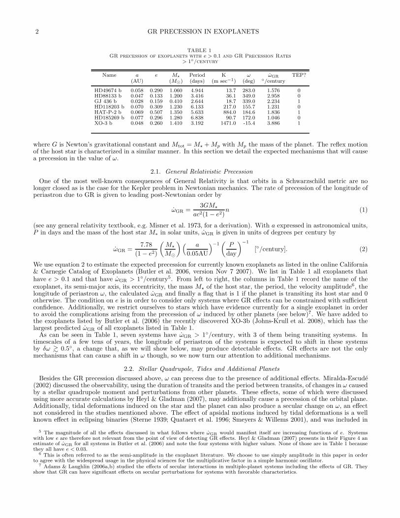
TABLE 1GR precession of exoplanets with e > 0.1 and GR Precession Rates

> 1◦/century

Name a e M⋆ Period K ω ωGR TEP?(AU) (M⊙) (days) (m sec−1) (deg) ◦/century

HD49674 b 0.058 0.290 1.060 4.944 13.7 283.0 1.576 0HD88133 b 0.047 0.133 1.200 3.416 36.1 349.0 2.958 0GJ 436 b 0.028 0.159 0.410 2.644 18.7 339.0 2.234 1HD118203 b 0.070 0.309 1.230 6.133 217.0 155.7 1.231 0HAT-P-2 b 0.069 0.507 1.350 5.633 884.0 184.6 1.836 1HD185269 b 0.077 0.296 1.280 6.838 90.7 172.0 1.046 0XO-3 b 0.048 0.260 1.410 3.192 1471.0 -15.4 3.886 1

where G is Newton’s gravitational constant and Mtot = M⋆ + Mp with Mp the mass of the planet. The reflex motionof the host star is characterized in a similar manner. In this section we detail the expected mechanisms that will causea precession in the value of ω.

2.1. General Relativistic Precession

One of the most well-known consequences of General Relativity is that orbits in a Schwarzschild metric are nolonger closed as is the case for the Kepler problem in Newtonian mechanics. The rate of precession of the longitude ofperiastron due to GR is given to leading post-Newtonian order by

ωGR =3GM⋆

ac2(1 − e2)n (1)

(see any general relativity textbook, e.g. Misner et al. 1973, for a derivation). With a expressed in astronomical units,P in days and the mass of the host star M∗ in solar units, ωGR is given in units of degrees per century by

ωGR =7.78

(1 − e2)

(

M⋆

M⊙

)

( a

0.05AU

)−1(

P

day

)−1

[◦/century]. (2)

We use equation 2 to estimate the expected precession for currently known exoplanets as listed in the online California& Carnegie Catalog of Exoplanets (Butler et al. 2006, version Nov 7 2007). We list in Table 1 all exoplanets thathave e > 0.1 and that have ωGR > 1◦/century5. From left to right, the columns in Table 1 record the name of theexoplanet, its semi-major axis, its eccentricity, the mass M⋆ of the host star, the period, the velocity amplitude6, thelongitude of periastron ω, the calculated ωGR and finally a flag that is 1 if the planet is transiting its host star and 0otherwise. The condition on e is in order to consider only systems where GR effects can be constrained with sufficientconfidence. Additionally, we restrict ourselves to stars which have evidence currently for a single exoplanet in orderto avoid the complications arising from the precession of ω induced by other planets (see below)7. We have added tothe exoplanets listed by Butler et al. (2006) the recently discovered XO-3b (Johns-Krull et al. 2008), which has thelargest predicted ωGR of all exoplanets listed in Table 1.

As can be seen in Table 1, seven systems have ωGR > 1◦/century, with 3 of them being transiting systems. Intimescales of a few tens of years, the longitude of periastron of the systems is expected to shift in these systemsby δω & 0.5◦, a change that, as we will show below, may produce detectable effects. GR effects are not the onlymechanisms that can cause a shift in ω though, so we now turn our attention to additional mechanisms.

2.2. Stellar Quadrupole, Tides and Additional Planets

Besides the GR precession discussed above, ω can precess due to the presence of additional effects. Miralda-Escude(2002) discussed the observability, using the duration of transits and the period between transits, of changes in ω causedby a stellar quadrupole moment and perturbations from other planets. These effects, some of which were discussedusing more accurate calculations by Heyl & Gladman (2007), may additionally cause a precession of the orbital plane.Additionally, tidal deformations induced on the star and the planet can also produce a secular change on ω, an effectnot considered in the studies mentioned above. The effect of apsidal motions induced by tidal deformations is a wellknown effect in eclipsing binaries (Sterne 1939; Quataert et al. 1996; Smeyers & Willems 2001), and was included in

5 The magnitude of all the effects discussed in what follows where ωGR would manifest itself are increasing functions of e. Systemswith low e are therefore not relevant from the point of view of detecting GR effects. Heyl & Gladman (2007) presents in their Figure 4 anestimate of ωGR for all systems in Butler et al. (2006) and note the four systems with higher values. None of those are in Table 1 becausethey all have e < 0.03.

6 This is often referred to as the semi-amplitude in the exoplanet literature. We choose to use simply amplitude in this paper in orderto agree with the widespread usage in the physical sciences for the multiplicative factor in a simple harmonic oscillator.

7 Adams & Laughlin (2006a,b) studied the effects of secular interactions in multiple-planet systems including the effects of GR. Theyshow that GR can have significant effects on secular perturbations for systems with favorable characteristics.

JORDAN & BAKOS 3

the analysis of the planetary system around HD 83443 by Wu & Goldreich (2002). Tidal deformations can produce asignificant amount of precession in close-in exoplanets and should therefore be taken into account.

The precession caused by a stellar quadrupole moment is given to second order in e and first order in (R∗/a)2 by

ωquad ≈ 3J2R2⋆

2a2n, (3)

where J2 is the quadrupole moment (Murray & Dermott 1999). In units of degree/century this expression reads

ωquad ≈ 0.17

(

P

day

)−1(J2

10−6

)(

R⋆

R⊙

)2( a

0.05AU

)−2

[◦/century]. (4)

It is clear from this equation that for values of J2 . 10−6 similar to that of the Sun (Pireaux & Rozelot 2003) thevalue of ωquad is smaller than the value of ω expected from GR (see also Miralda-Escude 2002). We will thereforeassume in what follows that ωquad is always negligible in comparison with ωGR.

The tidal deformations induced on the star and the planet by each other will lead to a change in the longitudeof periastron which is given, under the approximation that the objects can instantaneously adjust their equilibriumshapes to the tidal force and considering up to second order harmonic distortions, by

ωtide ≈15f(e)

a5

(

k2,sMpR5⋆

M⋆+

k2,pM⋆R5p

Mp

)

n, (5)

where f(e) ≡ (1 − e2)−5[1 + (3/2)e2 + (1/8)e4], and k2,s, k2,p are the apsidal motion constants for the star and planetrespectively, which depend on the mass concentration of the tidally deformed bodies (Sterne 1939). For stars we expectk2,s . 0.01 (Claret & Gimenez 1992), while for giant planets we expect k2,p ≈ 0.25 if we assume that their structurecan be roughly described by a polytrope of index n ≈ 1 (Hubbard 1984). For the extreme case of a sphere of uniformmass density, the apsidal motion constant takes the value k2 = 0.75 (e.g., Smeyers & Willems 2001). We see fromEquation 5 that for close-in hot Jupiters the term containing k2,p will dominate, and that the effect of tides on ωincreases very rapidly with decreasing a. In units of degree/century equation 5 gives

ωtide ≈ 1.6f(e)T(

P

day

)−1(k2,p

0.1

)

( a

0.05AU

)−5(

Rp

RJ

)5(MJ

Mp

)(

M⋆

M⊙

)

[◦/century], (6)

where we have introduced T ≡ 1 + (R⋆/Rp)5(Mp/M⋆)

2(k2,s/k2,p), which is ≈ 1 for the case of a close-in Jupiter.Assuming that k2,p ∼ 0.1, e . 0.5, Mp ∼ MJ , M⋆ ∼ M⊙, R⋆ ∼ R⊙ and Rp ∼ RJ it follows that ωtide is of comparablemagnitude as ωGR.

The precession of the periastra caused by a second planet, which we dub a “perturber”, is given to first order in eand lowest order in (a/a2) by

ωperturber ≈3M2a

3

4M⋆a32

n (7)

(Murray & Dermott 1999; Miralda-Escude 2002), where M2 is the mass of the second planet and a2 the semi-majoraxis of its orbit. In terms of deg/century this expression reads

ωperturber ≈ 29.6

(

P

day

)−1(a

a2

)3(M⋆

M⊙

)−1(M2

M⊕

)

[◦/century]. (8)

For a perturber with a2 = 2a and and a mass similar to Earth orbiting a solar-mass star, we get that ωperturber ∼3 × 10−7n or ωperturber ∼ 0.7 deg/century for a P = 5 days planet. This is comparable to the precession expectedfrom GR and therefore any detected precession of the longitude of periastron will be that of GR plus the possibleaddition of any perturber planet present in the system and the effects of tidal deformations (and generally a negligiblecontribution from the stellar quadrupole).

In what follows we will discuss the observability of changes in ω using radial velocity and transit observations. Asjust shown, any precession is expected to arise by GR, the effect of additional planets or tidal deformations. Thediscussion that follows addresses the detectability of changes in ω independent of their origin.

3. OBSERVABILITY OF PERIASTRA PRECESSION IN EXTRA-SOLAR PLANETS

3.1. Radial Velocities

The radial velocity of a star including the reflex motion due to a planetary component is given by

vr(t) = v0 + K[cos(ω + f(t − t0)) + e cos(ω)], (9)

where v0 is the systemic velocity, t0 the time coordinate zeropoint, f the true anomaly and K is the velocity amplitudewhich is related to the orbital elements and the masses by

K =

(

2πG

P

)1/3Mp sin i

Mtot, (10)

4 GR PRECESSION IN EXOPLANETS

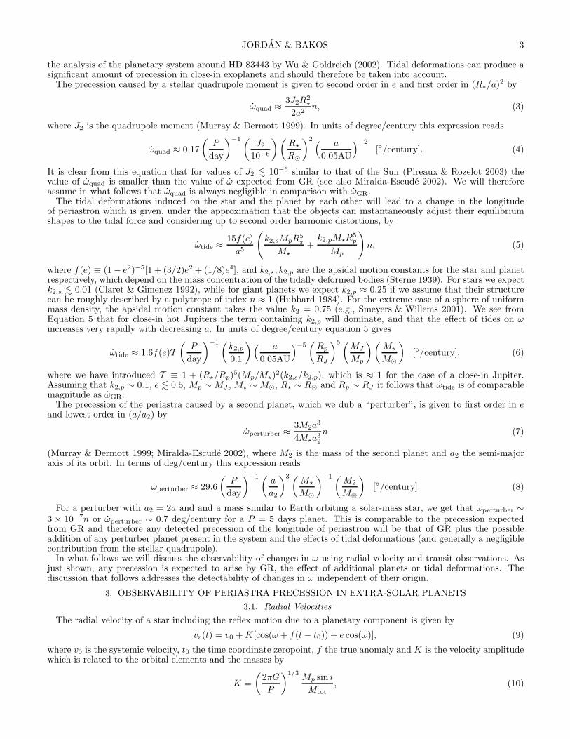
TABLE 2Results of Radial Velocity Curves Fit

Simulations for Nobs = 100, σobs = 2m/sec and σjitter = 4 m/sec

K e σω α20

(m sec−1) (deg) (deg/century)

100 0.10 3.77 80.010100 0.20 1.85 39.204100 0.30 1.29 27.457100 0.40 1.05 22.249100 0.50 0.95 20.253100 0.60 0.86 18.1591000 0.10 0.38 8.0591000 0.20 0.19 4.1061000 0.30 0.13 2.7681000 0.40 0.10 2.1821000 0.50 0.09 1.9591000 0.60 0.08 1.790

where i is the orbit inclination. Fitting for the observed radial velocities of a star will give then direct estimates ofv0, t0, K, e, P and ω.

Our aim in this section is to determine if ω can be constrained tightly enough in timescales of tens of years or lessin order to detect changes in ω of the magnitude produced by GR in those time-spans. In order to do this we havesimulated data and then fit it with a model of the form given by equation 9 a total of 1000 times. We then recoverthe best-fit values of ω in all simulations and use that to estimate the probability distribution φ(ω) expected undergiven assumptions.

The systemic velocity v0 and t0 are just zero-points that we set to 0 in all our simulations, where we also set thetime units such that P = 1 (note though that we do fit for all these quantities so that their effect on the fit propagatesto the uncertainties of ω). By trying several values of ω we have verified that the probability distributions recovereddo not depend strongly on the particular value of ω, which we therefore fix for all simulations at an arbitrary valueω0 = 135◦. This leaves us with just two parameters to vary, namely e and K.

Given e and K we generate Nobs data-points with times ti uniformly distributed8 within a period and then we addto each time a random number of periods between 0 and 20. For transiting exoplanets the observations would have tobe taken uniformly in time intervals excluding the transit. We then get the observed radial velocity from equation 9as

vr(ti) = K[cos(ω0 + f(ti)) + e cos(ω0)] + G(0, σtot) (11)

where G(0, σtot) is a random Gaussian deviate with mean 0 and standard deviation σtot. The latter quantity is obtainedas σ2

tot = σ2obs +σ2

jitter, where σobs is the random uncertainty for each measurement and σjitter is the noise arising fromstellar jitter. Given the form of equation 9 a Fisher matrix analysis implies that the uncertainty in the longitude ofperiastron, σω satisfies the following scaling

σω ∝ N−1/2obs σtotK

−1. (12)

This scaling allows us to perform a set of fiducial simulations for several values of e and use the results to scale toparameters relevant to a given situation of interest. We note that the simulations we performed verify that the scalinginferred from a Fisher matrix analysis is accurate. In order to measure the longitude of periastron ω with a reasonabledegree of certainty the system clearly needs to have a significant amount of eccentricity. We restrict ourselves tosystems with e ≥ 0.1 and we simulate systems with e = 0.1, 0.2, 0.3, 0.4, 0.5, 0.6.

For σobs we assume a typical high-precision measurement with σobs = 2 m sec−1. For the stellar jitter, we performour fiducial simulations for a typical jitter of σjitter = 4 m sec−1 (Wright 2005; Butler et al. 2006). The limitationsimposed by active stars and/or different precision on the radial velocity measurements on the recovery of ωGR can beexplored by using the scaling of σω with higher assumed values of σjitter and/or σobs. Even though Equation 12 rendersmultiple values of K redundant, we choose to present results for two values of K for illustrative purposes, namelyK = 100 m sec−1 and K = 1000 m sec−1. The former corresponds roughly to Jupiter-mass exoplanets and is fairlyrepresentative of currently known systems (Butler et al. 2006)9, while the latter corresponds to super-massive planetswhich as we will see are the class of systems which would allow the detection of ωGR with radial velocities. Finally, wedo our fiducial simulations for Nobs = 100, a value not atypical for well-sampled radial velocity curves available today.

The results of the simulations are summarized in Table 2. From left to right, the columns in this Table record theassumed radial velocity amplitude K, the system eccentricity e, the expected uncertainty in the longitude of periastron

8 We ignore in our simulations the Rossiter-McLaughlin effect for the case of transiting planets (Rossiter 1924; McLaughlin 1924;Queloz et al. 2000).

9 See also http://www.exoplanet.eu .

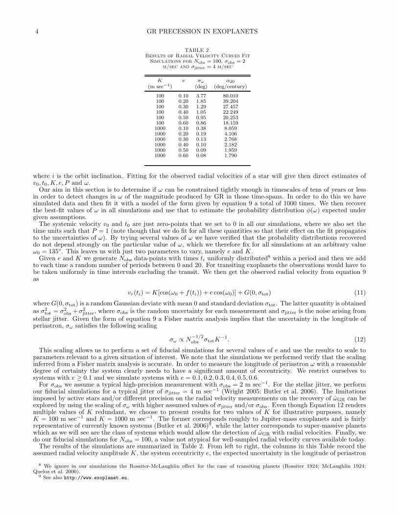
JORDAN & BAKOS 5

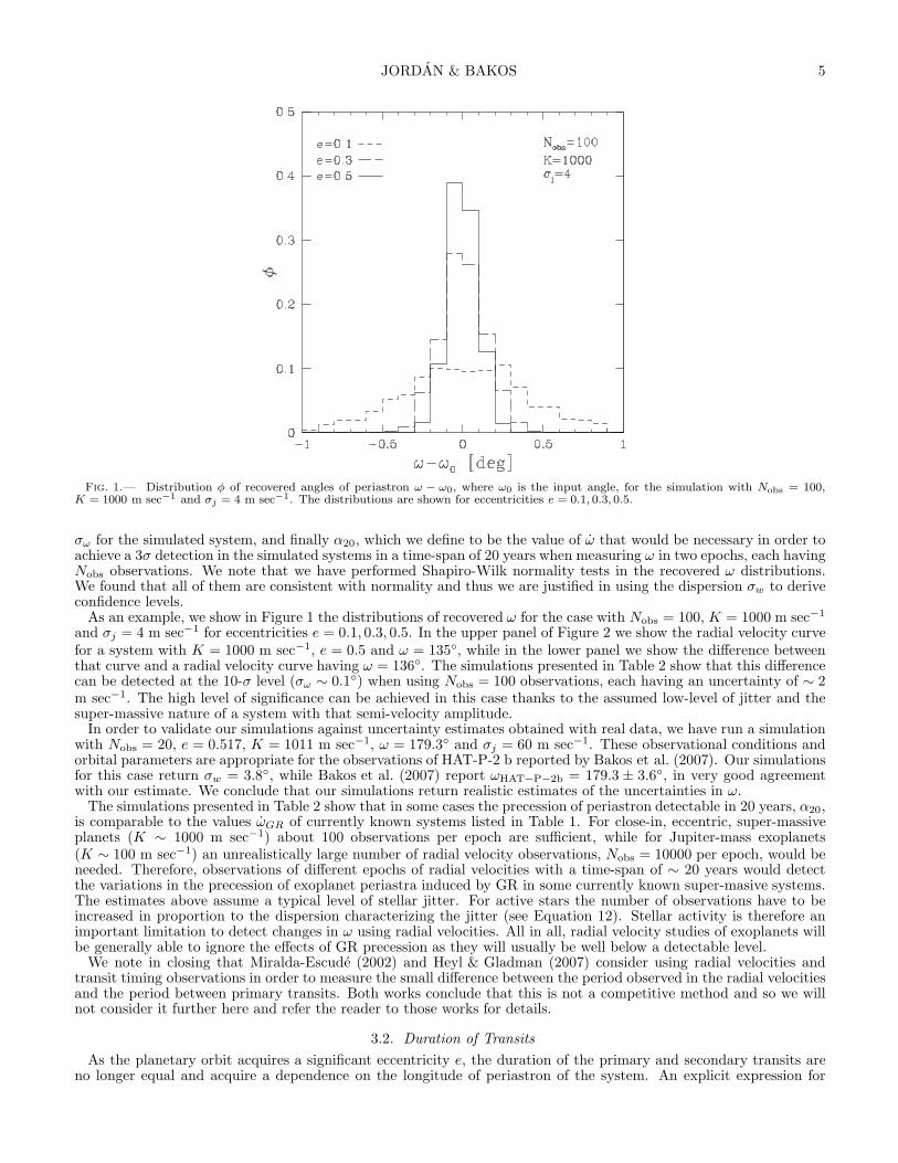
Fig. 1.— Distribution φ of recovered angles of periastron ω − ω0, where ω0 is the input angle, for the simulation with Nobs = 100,K = 1000 m sec−1 and σj = 4 m sec−1. The distributions are shown for eccentricities e = 0.1, 0.3, 0.5.

σω for the simulated system, and finally α20, which we define to be the value of ω that would be necessary in order toachieve a 3σ detection in the simulated systems in a time-span of 20 years when measuring ω in two epochs, each havingNobs observations. We note that we have performed Shapiro-Wilk normality tests in the recovered ω distributions.We found that all of them are consistent with normality and thus we are justified in using the dispersion σw to deriveconfidence levels.

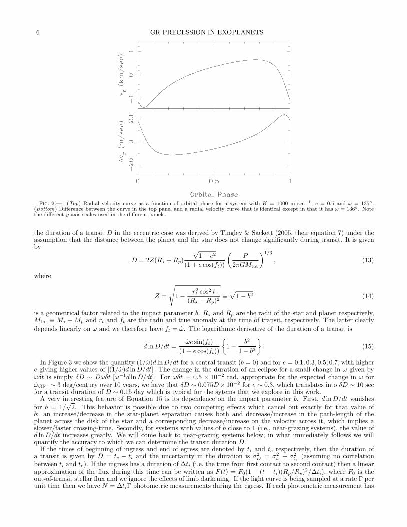
As an example, we show in Figure 1 the distributions of recovered ω for the case with Nobs = 100, K = 1000 m sec−1

and σj = 4 m sec−1 for eccentricities e = 0.1, 0.3, 0.5. In the upper panel of Figure 2 we show the radial velocity curvefor a system with K = 1000 m sec−1, e = 0.5 and ω = 135◦, while in the lower panel we show the difference betweenthat curve and a radial velocity curve having ω = 136◦. The simulations presented in Table 2 show that this differencecan be detected at the 10-σ level (σω ∼ 0.1◦) when using Nobs = 100 observations, each having an uncertainty of ∼ 2m sec−1. The high level of significance can be achieved in this case thanks to the assumed low-level of jitter and thesuper-massive nature of a system with that semi-velocity amplitude.

In order to validate our simulations against uncertainty estimates obtained with real data, we have run a simulationwith Nobs = 20, e = 0.517, K = 1011 m sec−1, ω = 179.3◦ and σj = 60 m sec−1. These observational conditions andorbital parameters are appropriate for the observations of HAT-P-2 b reported by Bakos et al. (2007). Our simulationsfor this case return σw = 3.8◦, while Bakos et al. (2007) report ωHAT−P−2b = 179.3 ± 3.6◦, in very good agreementwith our estimate. We conclude that our simulations return realistic estimates of the uncertainties in ω.

The simulations presented in Table 2 show that in some cases the precession of periastron detectable in 20 years, α20,is comparable to the values ωGR of currently known systems listed in Table 1. For close-in, eccentric, super-massiveplanets (K ∼ 1000 m sec−1) about 100 observations per epoch are sufficient, while for Jupiter-mass exoplanets(K ∼ 100 m sec−1) an unrealistically large number of radial velocity observations, Nobs = 10000 per epoch, would beneeded. Therefore, observations of different epochs of radial velocities with a time-span of ∼ 20 years would detectthe variations in the precession of exoplanet periastra induced by GR in some currently known super-masive systems.The estimates above assume a typical level of stellar jitter. For active stars the number of observations have to beincreased in proportion to the dispersion characterizing the jitter (see Equation 12). Stellar activity is therefore animportant limitation to detect changes in ω using radial velocities. All in all, radial velocity studies of exoplanets willbe generally able to ignore the effects of GR precession as they will usually be well below a detectable level.

We note in closing that Miralda-Escude (2002) and Heyl & Gladman (2007) consider using radial velocities andtransit timing observations in order to measure the small difference between the period observed in the radial velocitiesand the period between primary transits. Both works conclude that this is not a competitive method and so we willnot consider it further here and refer the reader to those works for details.

3.2. Duration of Transits

As the planetary orbit acquires a significant eccentricity e, the duration of the primary and secondary transits areno longer equal and acquire a dependence on the longitude of periastron of the system. An explicit expression for

6 GR PRECESSION IN EXOPLANETS

Fig. 2.— (Top) Radial velocity curve as a function of orbital phase for a system with K = 1000 m sec−1, e = 0.5 and ω = 135◦.(Bottom) Difference between the curve in the top panel and a radial velocity curve that is identical except in that it has ω = 136◦. Notethe different y-axis scales used in the different panels.

the duration of a transit D in the eccentric case was derived by Tingley & Sackett (2005, their equation 7) under theassumption that the distance between the planet and the star does not change significantly during transit. It is givenby

D = 2Z(R⋆ + Rp)

√1 − e2

(1 + e cos(ft))

(

P

2πGMtot

)1/3

, (13)

where

Z =

√

1 − r2t cos2 i

(R⋆ + Rp)2≡√

1 − b2 (14)

is a geometrical factor related to the impact parameter b. R⋆ and Rp are the radii of the star and planet respectively,Mtot ≡ M⋆ + Mp and rt and ft are the radii and true anomaly at the time of transit, respectively. The latter clearly

depends linearly on ω and we therefore have ft = ω. The logarithmic derivative of the duration of a transit is

d lnD/dt =ωe sin(ft)

(1 + e cos(ft))

{

1 − b2

1 − b2

}

. (15)

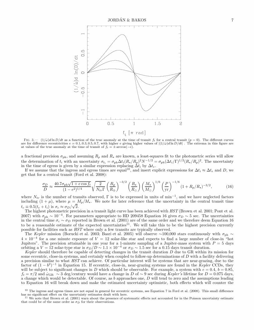
In Figure 3 we show the quantity (1/ω)d lnD/dt for a central transit (b = 0) and for e = 0.1, 0.3, 0.5, 0.7, with highere giving higher values of |(1/ω)d lnD/dt|. The change in the duration of an eclipse for a small change in ω given byωδt is simply δD ∼ Dωδt [ω−1d lnD/dt]. For ωδt ∼ 0.5 × 10−2 rad, appropriate for the expected change in ω forωGR ∼ 3 deg/century over 10 years, we have that δD ∼ 0.075D× 10−2 for e ∼ 0.3, which translates into δD ∼ 10 secfor a transit duration of D ∼ 0.15 day which is typical for the sytems that we explore in this work.

A very interesting feature of Equation 15 is its dependence on the impact parameter b. First, d lnD/dt vanishes

for b = 1/√

2. This behavior is possible due to two competing effects which cancel out exactly for that value ofb: an increase/decrease in the star-planet separation causes both and decrease/increase in the path-length of theplanet across the disk of the star and a corresponding decrease/increase on the velocity across it, which implies aslower/faster crossing-time. Secondly, for systems with values of b close to 1 (i.e., near-grazing systems), the value ofd lnD/dt increases greatly. We will come back to near-grazing systems below; in what immediately follows we willquantify the accuracy to which we can determine the transit duration D.

If the times of beginning of ingress and end of egress are denoted by ti and te respectively, then the duration ofa transit is given by D = te − ti and the uncertainty in the duration is σ2

D = σ2ti

+ σ2te

(assuming no correlationbetween ti and te). If the ingress has a duration of ∆ti (i.e. the time from first contact to second contact) then a linearapproximation of the flux during this time can be written as F (t) = F0(1 − (t − ti)(Rp/R⋆)

2/∆ti), where F0 is theout-of-transit stellar flux and we ignore the effects of limb darkening. If the light curve is being sampled at a rate Γ perunit time then we have N = ∆tiΓ photometric measurements during the egress. If each photometric measurement has

JORDAN & BAKOS 7

Fig. 3.— (1/ω)d lnD/dt as a function of the true anomaly at the time of transit ft for a central transit (p = 0). The different curvesare for difference eccentricities e = 0.1, 0.3, 0.5, 0.7, with higher e giving higher values of |(1/ω)d ln D/dt| . The extrema in this figure areat values of the true anomaly at the time of transit of ft = ± arccos(−e).

a fractional precision σph, and assuming Rp and R⋆ are known, a least-squares fit to the photometric series will allow

the determination of ti with an uncertainty σti= σph∆ti(R⋆/Rp)

2N−1/2 = σph(∆ti/Γ)1/2(R⋆/Rp)2. The uncertainty

in the time of egress is given by a similar expression replacing ∆ti by ∆te.If we assume that the ingress and egress times are equal10, and insert explicit expressions for ∆ti ≈ ∆te and D, we

get that for a central transit (Ford et al. 2008):

σD

D≈ 40.7σph

√1 + e cos ft

(1 − e2)1/4

√

2

NtrΓ

(

Rp

R⊕

)−3/2 (R⋆

R⊙

)(

M⋆

M⊙

)1/6 (P

yr

)−1/6

(1 + Rp/R⋆)−3/2, (16)

where Ntr is the number of transits observed, Γ is to be expressed in units of min−1, and we have neglected factorsincluding (1 + µ), where µ = Mp/M⋆. We note for later reference that the uncertainty in the central transit time

tc ≡ 0.5(te + ti) is σc ≈ σD/√

2.The highest photometric precision in a transit light curve has been achieved with HST (Brown et al. 2001; Pont et al.

2007) with σph ∼ 10−4. For parameters appropriate to HD 209458 Equation 16 gives σD ∼ 5 sec. The uncertaintiesin the central time σc ∼ σD reported in Brown et al. (2001) are of the same order and we therefore deem Equation 16to be a reasonable estimate of the expected uncertainties11. We will take this to be the highest precision currentlypossible for facilities such as HST where only a few transits are typically observed.

The Kepler mission (Borucki et al. 2003; Basri et al. 2005) will observe ∼100,000 stars continuously with σph ∼4 × 10−4 for a one minute exposure of V = 12 solar-like star and expects to find a large number of close-in “hotJupiters”. The precision attainable in one year for a 1-minute sampling of a Jupiter-mass system with P = 5 daysorbiting a V = 12 solar-type star is σD/D ∼ 1.1 × 10−4 or σD ∼ 1.5 sec for a 0.15 days transit duration.

Kepler should therefore be capable of detecting changes in the transit duration D due to GR within its mission forsome eccentric, close-in systems, and certainly when coupled to follow-up determinations of D with a facility deliveringa precision similar to what HST can achieve. Of particular interest will be systems that are near-grazing, due to thefactor of (1 − b2)−1 in Equation 15. If eccentric, close-in, near-grazing systems are found in the Kepler CCDs, theywill be subject to significant changes in D which should be observable. For example, a system with e = 0.4, b = 0.85,ft = π/2 and ωGR ∼ 3 deg/century would have a change in D of ∼ 9 sec during Kepler’s lifetime for D = 0.075 days,a change which would be detectable. Of course, as b approaches one, D will tend to zero and the assumptions leadingto Equation 16 will break down and make the estimated uncertainty optimistic, both effects which will counter the

10 The ingress and egress times are not equal in general for eccentric systems, see Equation 7 in Ford et al. (2008). This small differencehas no significant effect on the uncertainty estimates dealt with here.

11 We note that Brown et al. (2001) warn about the presence of systematic effects not accounted for in the Poisson uncertainty estimatethat could be of the same order as σD for their observations.

8 GR PRECESSION IN EXOPLANETS

corresponding increase of d lnD/dt.

3.3. Period Between Transits

As already noted by Miralda-Escude (2002) and Heyl & Gladman (2007), as the longitude of periastron changes, theperiod between transits Pt will change as well. Periods are the quantities that are measured with the greatest precision,usually with uncertainties on the order of seconds from ground-based observations (e.g., the average uncertainty forHATNet planets discovered to date is 4.5 seconds).

To first order in e the derivative of the transit period is given by

Pt = 4πe

(

ωGR

n

)2

sin(Mt) (17)

where Mt is the mean anomaly at transit (Miralda-Escude 2002) and is related to the true anomaly at transit ft tofirst order in e by Mt = ft − 2e sinft. For e = 0.1, a 5 day period, and ωGR = 3 deg/century, the root mean squarevalue of dPt/dt over all possible Mt values is ∼ 10−12, which translates into a period change of ∼ 2 × 10−4 sec in 10

years. The period can be determined to a precision ∼ σcN−3/2tr or σDN−1

tr 2−1/2 using the expression for σD above12.Assuming the parameters for Kepler as above (V = 12 star, P = 5 day period) the precision achievable during 1 yearis ∼ 0.013 sec.

Based on the numbers above we conclude that measuring significant changes in the transiting period in . 10 yearstimescales is not feasible. Our conclusions are in broad agreement with the analysis presented in Miralda-Escude(2002) and Heyl & Gladman (2007), who conclude that thousands of transits need to be observed with high precisionin order to detect significant variations in Pt. As there is no existing or planned facility that will allow to observethis amount of transits with the required photometric precision we conclude that measurements of Pt will not besignificantly affected by changes in ω of the magnitudes expected to arise from GR or from the secular changes due toa perturber.

3.4. Time Between Primary and Secondary Transit

In the case where the exoplanet is transiting it may be possible to observe not only the primary transit, i.e. the transitwhere the exoplanet obscures the host star, but also the occultation, when the host star blocks thermal emission andreflected light from the exoplanet (e.g., Charbonneau et al. 2005). If the time of the primary eclipse is given by t1 andthat of the secondary by t2, the time difference between the two as compared to half a period P , ∆t ≡ t2 − t1 − 0.5P ,depends mostly on the eccentricity e and the angle of periastron ω. Indeed, an accurate expression that neglects termsproportional to cot2 i where i is the inclination angle and is therefore exact for central transits, is given by

∆t =P

π

(

e cos(ω)√

1 − e2

(1 − (e sin ω)2)+ arctan

(

e cosω√1 − e2

)

)

(18)

(Sterne 1940). Combined with radial velocities this time difference offers an additional constrain on e and ω, and inprinciple a measurement of ∆t combined with a measurement of the difference in the duration of the secondary andprimary eclipses can be used to solve for e and ω directly (see discussion in Charbonneau et al. 2005). We note thatHeyl & Gladman (2007, their §4.2) also consider secondary transit timings as a means to measure changes in ω. Whiletheir discussion is based on first order expansions in e instead of using the exact expression above and is phrased indifferent terms, it is based ultimately on the same measurable quantity we discuss here. 13

Equation 18 does not include light travel time contributions, i.e. it neglects the time it takes for light to travelaccross the system. This time is given for a central transit by

∆t,LT =2a(1 − e2)

c[1 − (e cos ft)2], (19)

where ft is the true anomaly at the time of primary transit. In this section we will be interested in changes in ∆tdue to changes in ω. It is easy to see from the expressions above that d∆t,LT /dω ≪ d∆t/dω (ignoring the pointswhere they are both zero). Therefore, changes in the time difference between primary and secondary transits will bedominated by changes in ∆t and we can safely ignore light travel time effects in what follows.

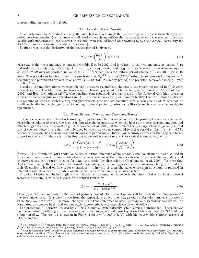
The precession of periastra caused by GR will change ω systematically, while leaving e unchanged. Therefore ∆thas the potential of offering a direct measurement of changes in ω. We use Equation 18 to calculate (1/P )d∆t/dω asa function of ω. The result is shown in in Figure 4 for e = 0.1, 0.3, 0.5, 0.7, with higher e yielding larger extrema of|(1/P )d∆t/dω|.

12 The scaling N−3/2 follows from describing the central transit times as ti = t0 + Pi, with i = 1, . . . , Ntr and determining P using aχ2 fit. The variance in the derived P is (see, e.g., Gould 2003) σ2

P ≈ (3/N3)σ2c + O(N−4).

13 Heyl & Gladman (2007) consider the time difference between successive primary transits (∆t0) and successive secondary (∆tπ) transits,following their notation. This difference can be expressed as ∆t0 − ∆tπ ≈ −(d∆t/dω)δω, where ∆t is the quantity defined in Equation 18and δω is the change in ω in one orbit.

JORDAN & BAKOS 9

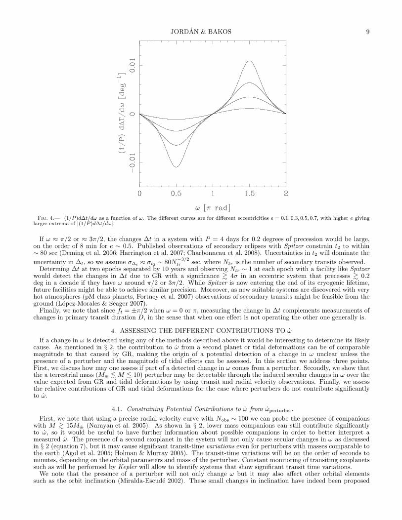
Fig. 4.— (1/P )d∆t/dω as a function of ω. The different curves are for different eccentricities e = 0.1, 0.3, 0.5, 0.7, with higher e givinglarger extrema of |(1/P )d∆t/dω|.

If ω ≈ π/2 or ≈ 3π/2, the changes ∆t in a system with P = 4 days for 0.2 degrees of precession would be large,on the order of 8 min for e ∼ 0.5. Published observations of secondary eclipses with Spitzer constrain t2 to within∼ 80 sec (Deming et al. 2006; Harrington et al. 2007; Charbonneau et al. 2008). Uncertainties in t2 will dominate the

uncertainty in ∆t, so we assume σ∆t≈ σt2 ∼ 80N

−3/2tr sec, where Ntr is the number of secondary transits observed.

Determing ∆t at two epochs separated by 10 years and observing Ntr ∼ 1 at each epoch with a facility like Spitzerwould detect the changes in ∆t due to GR with a significance & 4σ in an eccentric system that precesses & 0.2deg in a decade if they have ω around π/2 or 3π/2. While Spitzer is now entering the end of its cryogenic lifetime,future facilities might be able to achieve similar precision. Moreover, as new suitable systems are discovered with veryhot atmospheres (pM class planets, Fortney et al. 2007) observations of secondary transits might be feasible from theground (Lopez-Morales & Seager 2007).

Finally, we note that since ft = ±π/2 when ω = 0 or π, measuring the change in ∆t complements measurements ofchanges in primary transit duration D, in the sense that when one effect is not operating the other one generally is.

4. ASSESSING THE DIFFERENT CONTRIBUTIONS TO ω

If a change in ω is detected using any of the methods described above it would be interesting to determine its likelycause. As mentioned in § 2, the contribution to ω from a second planet or tidal deformations can be of comparablemagnitude to that caused by GR, making the origin of a potential detection of a change in ω unclear unless thepresence of a perturber and the magnitude of tidal effects can be assessed. In this section we address three points.First, we discuss how may one assess if part of a detected change in ω comes from a perturber. Secondly, we show thatthe a terrestrial mass (M⊕ . M . 10) perturber may be detectable through the induced secular changes in ω over thevalue expected from GR and tidal deformations by using transit and radial velocity observations. Finally, we assessthe relative contributions of GR and tidal deformations for the case where perturbers do not contribute significantlyto ω.

4.1. Constraining Potential Contributions to ω from ωperturber.

First, we note that using a precise radial velocity curve with Nobs ∼ 100 we can probe the presence of companionswith M & 15M⊕ (Narayan et al. 2005). As shown in § 2, lower mass companions can still contribute significantlyto ω, so it would be useful to have further information about possible companions in order to better interpret ameasured ω. The presence of a second exoplanet in the system will not only cause secular changes in ω as discussedin § 2 (equation 7), but it may cause significant transit-time variations even for perturbers with masses comparable tothe earth (Agol et al. 2005; Holman & Murray 2005). The transit-time variations will be on the order of seconds tominutes, depending on the orbital parameters and mass of the perturber. Constant monitoring of transiting exoplanetssuch as will be performed by Kepler will allow to identify systems that show significant transit time variations.

We note that the presence of a perturber will not only change ω but it may also affect other orbital elementssuch as the orbit inclination (Miralda-Escude 2002). These small changes in inclination have indeed been proposed

10 GR PRECESSION IN EXOPLANETS

as a method of detecting terrestrial mass companions in near-grazing transit systems which are especially sensitiveto them (Ribas et al. 2008). Following the formalism presented in §6 of Murray & Dermott (1999) we expect thatsecular changes to e by a perturber satisfy |de/dt| . (3/16)n(a/a2)

3(M2/M⋆)e2, where a2, e2 and M2 are the orbitalsemi-major axies, eccentricity and mass of the perturber respectively. For e2 = 0.1, a2 = 2a and M2 = 3 × 10−6M⋆

we have that de/dt . 4 × 10−6 yr−1 for a system with P = 4 days. This is too small for changes in e to be detectedwith radial velocities in scales of tens of years and so we conclude that secular changes in eccentricities induced byperturbers will in general not be useful to infer the presence of perturbers.

Summarizing, the best way to try to constrain contributions of ωperturber to a detected change in ω is to considertransiting systems posessing extensive photometric monitoring, allowing to probe the existence of transit time varia-tions. For near-grazing systems, the same photometric monitoring would additionally allow to probe for small changesin i due to a perturber.

4.2. Using Secular Variations in ω to Detect Terrestrial Mass Planets.

A very interesting possibility raised by the secular variation in ω induced by a “perturber” is to use these variations inorder to infer the presence of terrestrial mass planets. This possibility was studied by Miralda-Escude (2002) and thenfollowed-up by Heyl & Gladman (2007). Secular variations in ω, especially through their effect on transit durations(§ 3.2), can offer an interesting complement to transit time variations as a means of detecting terrestrial mass planetsin the upcoming Kepler mission.

As we have seen in § 2, the precession due to GR and tidal deformations can be of comparable magnitude to thatinduced by a terrestrial mass perturber. It is germane to ask then to what extent will the uncertainty in the expectedvalue of ωGR and ωtide limit the detectability of a perturber.

We start by considering ωGR . The fractional uncertainty in ωGR is given by (σ(ωGR )/ωGR )2 = (σ(M⋆)/M⋆)2 +

(σ(a)/a)2 + (σ(P )/P )2 + 4e2(σ(e)/(1 − e2))2, where we have ignored correlations. The fractional uncertainty in Pis generally negligible, while the other quantities can be typically of the order of a few percent. We will thereforeassume that σ(ωGR )/ωGR ∼ 10%. It follows that to detect an excess precession caused by a perturber we need atleast that ωperturber − ωGR & 0.3ωGR . It is easy to see that if ωperturber & ωGR and ωperturber is itself detectable, i.e.ωperturber > 3σω, where σω is the uncertainty in the measured ω, then the uncertainty in the expected ωGR will notspoil the significance of the detection. Using the equations presented in § 2 we get that

ωperturber

ωGR=

3.8

(1 − e2)

(

M⊙

M⋆

)2(a

a2

)3( a

0.05AU

)

(

M2

M⊕

)

. (20)

It is clear from this expression that for typical values of M⋆ ∼ M⊙, a ∼ 0.05 AU, e . 0.5 there will be values of a2

for which we have ωperturber > ωGR and for which the uncertainty in the expected precession from GR will not be alimiting factor in detecting terrestrial mass perturbers.

We consider now ωtide. The fractional uncertainty considering all parameters excepting k2,p and T and ignoringcorrelations is (σ(ωtide)/ωtide)

2 = (σ(P )/P )2 + (5σ(Rp/a)/(Rp/a))2 + (σ(Mp/M⋆)/(Mp/M⋆))2 + (f ′(e)σ(e)/f(e))2.

We have expressed this in terms of the ratios Mp/M⋆ and Rp/a as these quantities are more robustly determinedobservationally. As was the case above, the uncertainties in the variables can be typically a few percent and wetherefore assume that σ(ωtide)/ωtide ∼ 10%. Using the equations presented in § 2 we get that

ωperturber

ωtide=

1.85

T f(e)k2,p

(

M⊙

M⋆

)2(a

a2

)3( a

0.05AU

)5(

RJ

Rp

)5(Mp

MJ

)(

M2

M⊕

)

. (21)

In the case of ωtide we cannot measure the apsidal motion constant k2. As discussed in § 2, the value of k2 for a giantplanet is expected to be close to the extreme value of a uniform sphere, so we can conservatively assume k2,p = 0.75,a value that maximizes the expected ωtide. For a close-in Jupiter we have T ≈ 1. Using these values and followingthe same reasoning as for ωGR , it is clear from the expression above that for typical values of M⋆ ∼ M⊙, a ∼ 0.05AU, e . 0.5, Rp ∼ RJ , Mp ∼ MJ , there will be values of a2 for which we have ωperturber > ωtide and for whichthe uncertainty in the expected precession arising from tidal deformations will not be a limiting factor in detectingterrestrial mass perturbers. Note that due to the strong dependence on a, tides may become a limiting factor for veryclose-in systems.

We consider now the detectability of ωperturber with Kepler using the change in the transit duration D. As discussedin § 3.2, a 1-minute sampling of a Jupiter-mass system with Kepler for a P = 5 days planet orbiting a V = 12solar-type star will achieve a precision of σD ∼ 1.5 sec for a 0.15 days transit duration. We therefore set a changeof 6 sec over 4 years to constitute a detectable δD for this system, which translates into a detectable ω of ωdetect =6/(D∆t(ω−1d lnD/dt)), where ∆t = 4 years and we assume a central transit (see Equation 15).

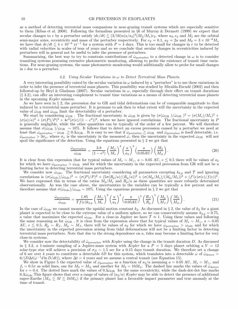
We show in Figure 5 the expected value of ωperturber as a function of a2/a assuming a = 0.05 AU, M⋆ = M⊙, andft = 0.5π as solid lines, one for M2 = M⊕ and another for M2 = 10M⊕. The dashed line marks the values of ωdetect

for e = 0.4. The dotted lines mark the values of 0.3ωGR for the same eccentricity, while the dash-dot-dot line marks0.3ωtide This figure shows that over a range of values of (a2/a) Kepler may be able to detect the presence of additionalsuper-Earths (M⊕ . M . 10M⊕) if the primary planet has a favorable impact parameter and true anomaly at thetime of transit.

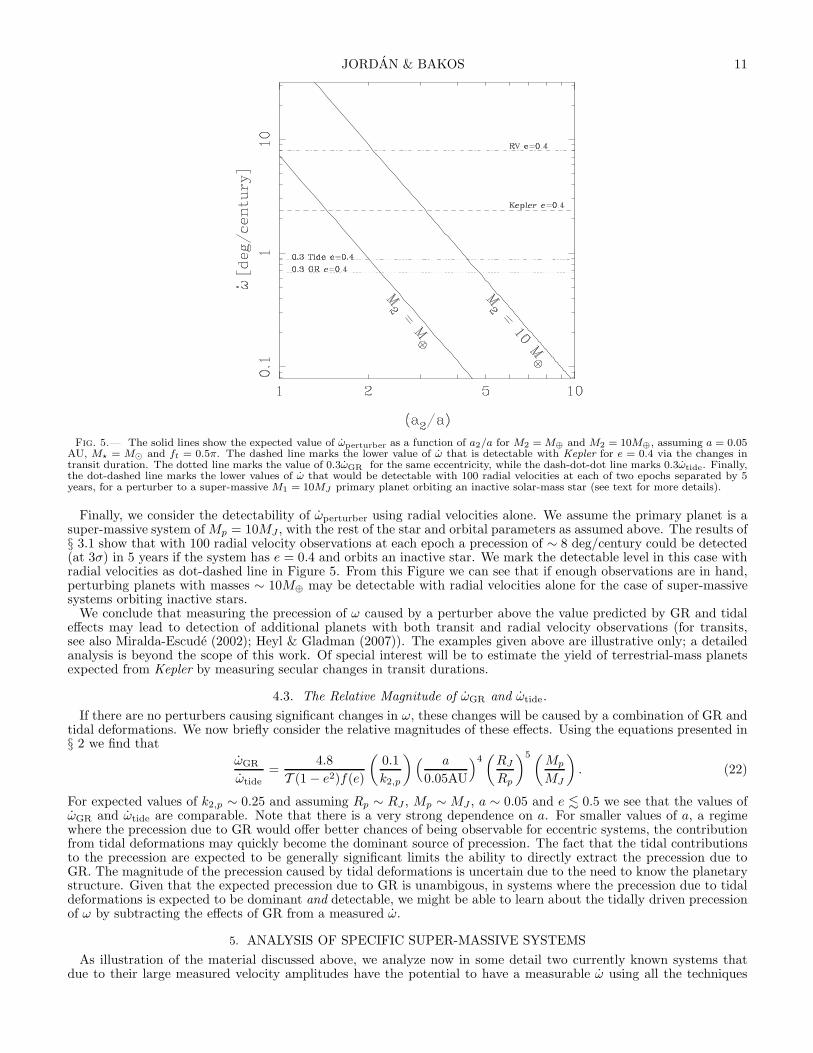
JORDAN & BAKOS 11

Fig. 5.— The solid lines show the expected value of ωperturber as a function of a2/a for M2 = M⊕ and M2 = 10M⊕, assuming a = 0.05AU, M⋆ = M⊙ and ft = 0.5π. The dashed line marks the lower value of ω that is detectable with Kepler for e = 0.4 via the changes intransit duration. The dotted line marks the value of 0.3ωGR for the same eccentricity, while the dash-dot-dot line marks 0.3ωtide. Finally,the dot-dashed line marks the lower values of ω that would be detectable with 100 radial velocities at each of two epochs separated by 5years, for a perturber to a super-massive M1 = 10MJ primary planet orbiting an inactive solar-mass star (see text for more details).

Finally, we consider the detectability of ωperturber using radial velocities alone. We assume the primary planet is asuper-massive system of Mp = 10MJ , with the rest of the star and orbital parameters as assumed above. The results of§ 3.1 show that with 100 radial velocity observations at each epoch a precession of ∼ 8 deg/century could be detected(at 3σ) in 5 years if the system has e = 0.4 and orbits an inactive star. We mark the detectable level in this case withradial velocities as dot-dashed line in Figure 5. From this Figure we can see that if enough observations are in hand,perturbing planets with masses ∼ 10M⊕ may be detectable with radial velocities alone for the case of super-massivesystems orbiting inactive stars.

We conclude that measuring the precession of ω caused by a perturber above the value predicted by GR and tidaleffects may lead to detection of additional planets with both transit and radial velocity observations (for transits,see also Miralda-Escude (2002); Heyl & Gladman (2007)). The examples given above are illustrative only; a detailedanalysis is beyond the scope of this work. Of special interest will be to estimate the yield of terrestrial-mass planetsexpected from Kepler by measuring secular changes in transit durations.

4.3. The Relative Magnitude of ωGR and ωtide.

If there are no perturbers causing significant changes in ω, these changes will be caused by a combination of GR andtidal deformations. We now briefly consider the relative magnitudes of these effects. Using the equations presented in§ 2 we find that

ωGR

ωtide=

4.8

T (1 − e2)f(e)

(

0.1

k2,p

)

( a

0.05AU

)4(

RJ

Rp

)5(Mp

MJ

)

. (22)

For expected values of k2,p ∼ 0.25 and assuming Rp ∼ RJ , Mp ∼ MJ , a ∼ 0.05 and e . 0.5 we see that the values ofωGR and ωtide are comparable. Note that there is a very strong dependence on a. For smaller values of a, a regimewhere the precession due to GR would offer better chances of being observable for eccentric systems, the contributionfrom tidal deformations may quickly become the dominant source of precession. The fact that the tidal contributionsto the precession are expected to be generally significant limits the ability to directly extract the precession due toGR. The magnitude of the precession caused by tidal deformations is uncertain due to the need to know the planetarystructure. Given that the expected precession due to GR is unambigous, in systems where the precession due to tidaldeformations is expected to be dominant and detectable, we might be able to learn about the tidally driven precessionof ω by subtracting the effects of GR from a measured ω.

5. ANALYSIS OF SPECIFIC SUPER-MASSIVE SYSTEMS

As illustration of the material discussed above, we analyze now in some detail two currently known systems thatdue to their large measured velocity amplitudes have the potential to have a measurable ω using all the techniques

12 GR PRECESSION IN EXOPLANETS

presented above: HAT-P-2 b (Bakos et al. 2007; Loeillet et al. 2008) and XO-3 b (Johns-Krull et al. 2008).

5.1. HAT-P-2 b

HAT-P-2 b is an especially interesting system due to its very high eccentricity, high mass of ≈ 9MJ and close orbit(a = 0.0677 AU) to its host star. As shown in Table 1 its value of ωGR is ∼ 2◦/century, while the expected value ofωtide is ∼ 0.25 deg/century assuming k2,p = 0.25. Unfortunately it has a high level of stellar jitter, with estimatesranging from 17 m sec−1 to 60 m sec−1 (Bakos et al. 2007; Loeillet et al. 2008). So even though this system has K ∼1000 m sec−1 it would require an unrealistically large number of observations (∼ 104) per epoch in order to make itsexpected ωGR detectable with radial velocities.

The value of ω derived for HAT-P-2 b is 1.05π and we therefore would not expect to see significant variations inthe time between primary and secondary transits in case the secondary transit was observed (see Figure 4). Withω = 1.05π the true anomaly at the time of transit will be ft ≈ 0.45π, or 1.55π. Given that the impact parameter isb ≈ 0 we get from Equation 15 that |d ln D/dt| ∼ 1.67× 10−2 century−1. Using the fact that D = 0.15 days we expectthen a change of ∼ 21 sec in D over 10 years due to GR. This difference could be readily detected with high precisionphotometric observations that determine D to within a few seconds such as is possible with HST. The observationscurrently available constrain D only to within ∼ 3 mins (Bakos et al. 2007), and so no first epoch suitable to measuringchanges in D is yet in hand.

5.2. XO-3 b

As shown in Table 1 XO-3 b has the largest predicted ωGR of all currently known exoplanets with e > 0.1. Whileits eccentricity is not as high as that of HAT-P-2 b, it is more massive and orbits closer to its host star XO-3 (alsoknown as GSC 03727-01064). Asuming k2,p = 0.25, the expected value of ωtide is ∼ 11 deg/century, about three timesas much as the contribution from GR.

In order to assess the detectability of ω with radial velocities for XO-3 b we need to know σjitter, but unfortunatelythe precision of the radial velocity measurements presented in Johns-Krull et al. (2008) is too coarse to allow a deter-mination of this quantity (σobs & 100 m sec−1). Based on the spectral type F5V and v sin i = 18.5 ± 0.2 km sec−1

of XO-3 b (Johns-Krull et al. 2008) we can expect it to have a rather high value of stellar jitter σjitter & 30 m sec−1

(Saar et al. 1998). Therefore, and just as is the case for HAT-P-2 b, we do not expect ω to be detectable with radialvelocity observations due to the expected jitter.

The value of ω derived for XO-3 b is consistent with 0 and we therefore would not expect to see variations in thetime between primary and secondary transits in case the secondary transit was observed (see Figure 4). As ω ≈ 0, thetrue anomaly at the time of transit will be ft ≈ π/2 or 3π/2. Given that the impact parameter is b ≈ 0.8 we get fromEquation 15 that |d lnD/dt| ∼ 3.56 × 10−2 century−1. Using the fact that D = 0.14 days we expect then a change of∼ 43 sec in D over 10 years. Just as is the case for HAT-P-2 b, this could be detectable with determinations of D towithin a few seconds and there is no suitable first epoch yet in hand.

6. CONCLUSIONS

In this work we have studied the observability of the precession of periastra caused by general relativity in exoplanets.We additionally consider the precession caused by tidal deformations and planetary perturbers, which can produce aprecession of comparable or greater magnitude. We consider radial velocities and transit light curve observations andconclude that for some methods precessions of the magnitude expected from GR will be detectable in timescales of∼ 10 years or less for some close-in, eccentric systems. In more detail, we find that:

1. For transiting systems, precession of periastra of the magnitude expected from GR will manifest itself throughdetectable changes in the duration of primary transit (§3.2) or through the change in the time between primaryand secondary transits (§3.4) in timescales of . 10 years. The two methods are most effective at different valuesof the true anomaly. A determination of the primary transit duration time to ∼ a few seconds and that of thesecondary to ∼ a minute will lead to measurable effects. The effects of GR and tidal deformations might needto be included in the analysis of Kepler data for eccentric, close-in systems. The transit duration of near-grazingsystems will be particulary sensitive to changes in ω.

2. Radial velocity observations alone would be able to detect changes in the longitude of periastron of the magnitudeexpected from GR effects only for eccentric super-massive (K ∼ 1000 m sec−1) exoplanets orbiting close to ahost star with a low-level of stellar jitter (§3.1). For the detection to be statistically significant, on the order of100 precise radial velocity observations are needed at each of two epochs separated by ∼ 20 years.

3. Measurements of the change over time of the period between primary transits is not currently a method that willlead to a detection of changes in ω of the magnitude expected from GR (§3.3). Previous works have shown thatmeasuring the small difference between the radial velocity period and that of transits are not sensitive enoughto lead to detectable changes due to GR.

In order to contrast any detected change in the transit duration (§3.2) or the time between primary and secondary(§3.4) to the predictions of a given mechanism one needs to know the eccentricity and longitude of periastron of the

JORDAN & BAKOS 13

systems, for which radial velocities are needed (although not necessarily of the precision required to directly detectchanges in ω with them14). Conversely, photometric monitoring of primary transits are useful in order to elucidate thenature of a detected change in ω by probing for the presence of transit time variations. The presence of the latter wouldimply that at least part of any observed changes in ω could have been produced by additional planetary companions(§4).

Precession of periastra caused by planetary perturbers and the effects of tidal deformations can be of comparablemagnitude to that caused by GR (§2.2). The effects of tidal deformations on the precession of periastra in particularmay be of the same magnitude or dominate the total ω in the regime where the GR effects are detectable (§4.3). Whilethis limits the ability to directly extract the precession due to GR given the uncertainty in the expected precession fromtides, it might allow to study the tidally induced precession by considering the residual precession after subtractingthe effects of GR. The latter possibility is particularly attractive in systems where the tidally induced precessionmay dominate the signal. We note that even without considering the confusing effects of tidal contributions to theprecession, a measurement of ωGR as described in this work would not be competitive in terms of precision with binarypulsar studies (see, e.g., Will 2006, for a review ) and would therefore not offer new tests of GR.

The upcoming Kepler mission expects to find a large number of massive planets transiting close to their host stars(Borucki et al. 2003), some of which will certainly have significant eccentricities. Furthermore, systems observed byKepler will be extensively monitored for variations in their transiting time periods in order to search for terrestrial-mass planets using transit-time variations. We have shown that modeling of the transit time durations and furthercharacterization of close-in, eccentric systems might need to take into account the effects of GR and tidal deformationsas they will become detectable on timescales comparable to the 4-year lifetime of the mission, and certainly on follow-up studies after the mission ends. We have also shown that planetary companions with super-Earth masses may bedetectable by Kepler by the change in transit durations they induce (§ 4.2). Additionally, well sampled radial velocitycurves spanning & 5 years may also be able to detect companions with super-earth massses by measuring a change inω over the expected GR value for the case of super-massive, close-in systems orbiting inactive stars (§ 4.2).

We would like to thank the anonymous referee for helpful suggestions and Dan Fabrycky and Andras Pal for usefuldiscussions. G.B. acknowledges support provided by the National Science Foundation through grant AST-0702843.

REFERENCES

Adams, F. C., & Laughlin, G. 2006a, ApJ, 649, 992—. 2006b, ApJ, 649, 1004Agol, E., Steffen, J., Sari, R., & Clarkson, W. 2005, MNRAS,

359, 567

Bakos, G. A., Kovacs, G., Torres, G., Fischer, D. A., Latham,D. W., Noyes, R. W., Sasselov, D. D., Mazeh, T., Shporer, A.,Butler, R. P., Stefanik, R. P., Fernandez, J. M., Sozzetti, A.,Pal, A., Johnson, J., Marcy, G. W., Winn, J. N., Sipocz, B.,Lazar, J., Papp, I., & Sari, P. 2007, ApJ, 670, 826

Basri, G., Borucki, W. J., & Koch, D. 2005, New AstronomyReview, 49, 478

Borucki, W. J., Koch, D. G., Basri, G. B., Caldwell, D. A.,Caldwell, J. F., Cochran, W. D., Devore, E., Dunham, E. W.,Geary, J. C., Gilliland, R. L., Gould, A., Jenkins, J. M.,Kondo, Y., Latham, D. W., & Lissauer, J. J. 2003, inAstronomical Society of the Pacific Conference Series, Vol. 294,Scientific Frontiers in Research on Extrasolar Planets, ed.D. Deming & S. Seager, 427–440

Brown, T. M., Charbonneau, D., Gilliland, R. L., Noyes, R. W.,& Burrows, A. 2001, ApJ, 552, 699

Butler, R. P., Marcy, G. W., Williams, E., Hauser, H., & Shirts,P. 1997, ApJ, 474, L115

Butler, R. P., Wright, J. T., Marcy, G. W., Fischer, D. A., Vogt,S. S., Tinney, C. G., Jones, H. R. A., Carter, B. D., Johnson,J. A., McCarthy, C., & Penny, A. J. 2006, ApJ, 646, 505

Charbonneau, D., Allen, L. E., Megeath, S. T., Torres, G.,Alonso, R., Brown, T. M., Gilliland, R. L., Latham, D. W.,Mandushev, G., O’Donovan, F. T., & Sozzetti, A. 2005, ApJ,626, 523

Charbonneau, D., Knutson, H. A., Barman, T., Allen, L. E.,Mayor, M., Megeath, S. T., Queloz, D., & Udry, S. 2008, ArXive-prints arXiv:0802.0845

Claret, A., & Gimenez, A. 1992, A&AS, 96, 255Deming, D., Harrington, J., Seager, S., & Richardson, L. J. 2006,

ApJ, 644, 560Ford, E. B., Quinn, S. N., & Veras, D. 2008, ApJ, 678, 1407Fortney, J. J., Lodders, K., Marley, M. S., & Freedman, R. S.

2007, ArXiv e-prints arXiv:0710.2558Goldreich, P., & Soter, S. 1966, Icarus, 5, 375Gould, A. 2003, ArXiv Astrophysics e-prints astro-ph/0310577Harrington, J., Luszcz, S., Seager, S., Deming, D., & Richardson,

L. J. 2007, Nature, 447, 691Heyl, J. S., & Gladman, B. J. 2007, MNRAS, 377, 1511

Holman, M. J., & Murray, N. W. 2005, Science, 307, 1288Hubbard, W. B. 1984, Planetary interiors (New York, Van

Nostrand Reinhold Co., 1984, 343 p.)

Johns-Krull, C. M., McCullough, P. R., Burke, C. J., Valenti,J. A., Janes, K. A., Heasley, J. N., Prato, L., Bissinger, R.,Fleenor, M., Foote, C. N., Garcia-Melendo, E., Gary, B. L.,Howell, P. J., Mallia, F., Masi, G., & Vanmunster, T. 2008,ApJ, 677, 657

Loeillet, B., Shporer, A., Bouchy, F., Pont, F., Mazeh, T., Beuzit,J. L., Boisse, I., Bonfils, X., da Silva, R., Delfosse, X., Desort,M., Ecuvillon, A., Forveille, T., Galland, F., Gallenne, A.,Hebrard, G., Lagrange, A.-M., Lovis, C., Mayor, M., Moutou,C., Pepe, F., Perrier, C., Queloz, D., Segransan, D., Sivan,J. P., Santos, N. C., Tsodikovich, Y., Udry, S., &Vidal-Madjar, A. 2008, A&A, 481, 529

Lopez-Morales, M., & Seager, S. 2007, ApJ, 667, L191Marcy, G. W., & Butler, R. P. 1996, ApJ, 464, L147+Mayor, M., & Queloz, D. 1995, Nature, 378, 355McLaughlin, D. B. 1924, ApJ, 60, 22Miralda-Escude, J. 2002, ApJ, 564, 1019Misner, C. W., Thorne, K. S., & Wheeler, J. A. 1973, Gravitation

(San Francisco: W.H. Freeman and Co., 1973)Murray, C. D., & Dermott, S. F. 1999, Solar system dynamics

(Cambridge: Cambridge University Press, 1999)Narayan, R., Cumming, A., & Lin, D. N. C. 2005, ApJ, 620, 1002Pal, A., & Kocsis, B. 2008, MNRAS, in pressPireaux, S., & Rozelot, J.-P. 2003, Ap&SS, 284, 1159Pont, F., Gilliland, R. L., Moutou, C., Charbonneau, D., Bouchy,

F., Brown, T. M., Mayor, M., Queloz, D., Santos, N., & Udry,S. 2007, A&A, 476, 1347

Quataert, E. J., Kumar, P., & Ao, C. O. 1996, ApJ, 463, 284Queloz, D., Eggenberger, A., Mayor, M., Perrier, C., Beuzit,

J. L., Naef, D., Sivan, J. P., & Udry, S. 2000, A&A, 359, L13Rasio, F. A., Tout, C. A., Lubow, S. H., & Livio, M. 1996, ApJ,

470, 1187Ribas, I., Font-Ribera, A., & Beaulieu, J.-P. 2008, ApJ, 677, L59Rossiter, R. A. 1924, ApJ, 60, 15Saar, S. H., Butler, R. P., & Marcy, G. W. 1998, ApJ, 498, L153+Smeyers, P., & Willems, B. 2001, A&A, 373, 173Sterne, T. E. 1939, MNRAS, 99, 451—. 1940, Proceedings of the National Academy of Science, 26, 36Tingley, B., & Sackett, P. D. 2005, ApJ, 627, 1011Will, C. M. 2006, Living Reviews in Relativity, 9Wright, J. T. 2005, PASP, 117, 657Wu, Y., & Goldreich, P. 2002, ApJ, 564, 1024

14 GR PRECESSION IN EXOPLANETS

14 The eccentricity can be constrained using transit information alone, see Ford et al. (2008)