object matching in disjoint cameras using a color transfer approach

ABSTRACT OF THESIS

OBJECT MATCHING IN DISJOINT CAMERASUSING A COLOR TRANSFER APPROACH

Object appearance models are a consequence of illumination, viewing direction, cam-era intrinsics, and other conditions that are specific to a particular camera. As aresult, a model acquired in one view is often inappropriate for use in other viewpoints.In this work we treat this appearance model distortion between two non-overlappingcameras as one in which some unknown color transfer function warps a known appear-ance model from one view to another. We demonstrate how to recover this functionin the case where the distortion function is approximated as general affine and objectappearance is represented as a mixture of Gaussians. Appearance models are broughtinto correspondence by searching for a bijection function that best minimizes an en-tropic metric for model dissimilarity. These correspondences lead to a solution for thetransfer function that brings the parameters of the models into alignment in the UVchromaticity plane. Finally, a set of these transfer functions acquired from a collec-tion of object pairs are generalized to a single camera-pair-specific transfer functionvia robust fitting. We demonstrate the method in the context of a video surveillancenetwork and show that recognition of subjects in disjoint views can be significantlyimproved using the new color transfer approach.

KEYWORDS: Computer Vision, Wide-Area Multi-Camera Surveillance Network, Ob-ject Matching, Color, Appearance Model

Copyright c© Kideog Jeong 2006

Kideog Jeong

November 27th, 2006


By

Kideog Jeong

Director of Thesis

Director of Graduate Studies

RULES FOR THE USE OF DISSERTATIONS

Unpublished dissertations submitted for the Doctor’s degree and deposited in theUniversity of Kentucky Library are as a rule open for inspection, but are to be usedonly with due regard to the rights of the authors. Bibliographical references maybe noted, but quotations or summaries of parts may be published only with thepermission of the author, and with the usual scholarly acknowledgements.

Extensive copying or publication of the dissertation in whole or in part also requiresthe consent of the Dean of the Graduate School of the University of Kentucky.

A library that borrows this dissertation for use by its patrons is expected to securethe signature of each user.

Name Date

THESIS

Kideog Jeong

The Graduate School

University of Kentucky

2006


THESIS

A thesis submitted in partial fulfillment of therequirements for the degree of Master of Science in the

College of Engineeringat the University of Kentucky

By

Kideog Jeong

Lexington, Kentucky

Director: Dr. Christopher Jaynes, Associate Professor of Computer

Science

Lexington, Kentucky

2006


ACKNOWLEDGEMENTS

First, I would like to especially thank my advisor, Professor Christopher Jaynes with-

out whom this thesis would not exist. I am grateful to him for his constant encour-

agement and guidance through teaching, research and writing required to bring this

thesis to completion. My first opportunity to have interests to the area of computer

vision was his great class titled as “Situated Computing” that helped to make com-

puter vision fun for me. In research, he has lots of great ideas regarding wide-area

multi-camera systems. This thesis work has been done as part of the ambient virtual

assistant (AVA) that he proposed. I will be forever in his debt of the support and

encouragement that he has provided me throughout my graduate career.

My appreciation goes to my other committee members as well. I thank Dr. Amit

Kale for technical discussions on this thesis and precious advice on computer vision

research in general. He put a stress on the importance of statistical inference and

introduced me to many helpful articles related to illumination invariant vision. I also

thank Dr. Sen-ching “Samson” Cheung for kindly accepting the role of the committee.

He introduced me to new knowledge on probabilistic graphical models that are playing

an increasingly important role in diverse areas such as communication, bioinformatics,

computer vision, neuroscience, and economics. Thanks to all of you not just for being

on my committee but for all of your guidance and assistance.

I owe a great deal to the members of the Metaverse Computer Vision lab and the

staffs of the UK visualization center in many ways. Especially, I thank Nathaniel

Sanders and the many other researchers for sharing their hard worked computer

programs such as EasyCamera, multi-camera image grabber and so forth.

Lastly, to my wife, Eun-Joo Lee and my parents: thank you for your patience,

support, and all the other things that make it so worthwhile to have this thesis.

iii

Table of Contents

Acknowledgements iii

Table of Contents iv

List of Tables v

List of Figures vi

List of Files i

1 Introduction 11.1 Problem Description and Methodology . . . . . . . . . . . . . . . . . 51.2 Assumptions . . . . . . . . . . . . . . . . . . . . . . . . . . . . . . . . 61.3 Contributions . . . . . . . . . . . . . . . . . . . . . . . . . . . . . . . 7

2 Technical Details 92.1 Component-wise similarity metric using bijective mapping in chro-

maticity space . . . . . . . . . . . . . . . . . . . . . . . . . . . . . . . 102.2 Estimating the parameters of color transfer function . . . . . . . . . . 132.3 Refining the color transfer function . . . . . . . . . . . . . . . . . . . 16

3 Experimental results 193.1 Multi-camera dataset . . . . . . . . . . . . . . . . . . . . . . . . . . . 193.2 Object pixel classification . . . . . . . . . . . . . . . . . . . . . . . . 213.3 Direct comparison to other techniques . . . . . . . . . . . . . . . . . 24

4 Discussion 28

5 Conclusions and Future Work 325.1 Future Work . . . . . . . . . . . . . . . . . . . . . . . . . . . . . . . . 32

Bibliography 33

Vita 37

iv

List of Tables

1.1 Comparison of the technical components used Javed et al. [29] and our method. 5

3.1 Confusion matrix for all eight subjects seen throughout the experiment.Table contains true positive rates without applying the appropriatecolor transfer functions. . . . . . . . . . . . . . . . . . . . . . . . . . 20

3.2 Confusion matrix for all eight subjects observed in the experimentwhen using the derived color transfer functions. Table shows true pos-itive rates for each subject. The use of color transfer functions leadsto an overall improvement of over 50%. . . . . . . . . . . . . . . . . . 21

v

List of Figures

1.1 The same subject observed in two views (a-b), is illuminated differ-ently with different camera intrinsics, and under different pose in asurveillance network. This leads to a change in chromaticity samplesmeasured on the moving object. (c-d). This deformation should betaken into account to support persistent object tracking in multipleviews. . . . . . . . . . . . . . . . . . . . . . . . . . . . . . . . . . . . 2

2.1 Assignment of model component correspondence is important to ac-curate transfer function estimation. Two models are plotted on thesame chromaticity plane. (a) Straightforward pair-wise similarity met-ric using Ψ1 can lead to a false bijective map (γa(i) = (2, 1, 3)) whenD(Θ, Θ, γa) ≤ D(Θ, Θ, γb) where γb(i) = (1, 2, 3) is considered to betrue bijective map. (b) This is avoided by utilizing characteristics ofthe chromaticity plane where the achromatic locus acts as the polar ori-gin. The relative entropy between each proposed correspondence andan achromatic distribution (θC) at this point is taken into account (seeText). (c) Relative orientation with respect to the achromatic locusresolves ambiguities arising from two models whose relative distancesto θC are uniform. . . . . . . . . . . . . . . . . . . . . . . . . . . . . . 11

3.1 A typical camera transition from camera 3 to camera 5 shown inimages (a) and (b) respectively. (c) Classification result when all pixelsin motion from camera 5 are compared directly to appearance modelderived in camera 3. White pixels correspond to chromaticity sampleswithin a Mahalanobis distance of less than 1.5. (d) By first applyingthe color transfer function from camera 3 to camera 5, classificationresults improve dramatically. . . . . . . . . . . . . . . . . . . . . . . . 22

3.2 Result of two views of subject F under dramatically different illumi-nation conditions. Subject F’s transition is shown in (a) and (b). (c)and (d) display enlarged sections of chromaticity samples of the sub-ject shown in (a) and (b) respectively. Note that the different axisscales are used for clarity. Solid ellipses represent the components ofthe color model. In (d), dotted ellipses depict the recovered deforma-tion parameters of the model shown in (c). (e) and (f) are the pixelclassification result without/with transforming the model in view (a)respectively. . . . . . . . . . . . . . . . . . . . . . . . . . . . . . . . . 23

3.3 Performance comparison of object different matching methods as com-pared to the approach introduced here. Graph shows the true positiverates (y axis) versus the number of objects (x axis). The solid anddashed curves denote with/without the RGB diagonal color correction(CC) respectively. CTF stands for the color transfer function method. 26

3.4 The Φ error measure between each object and itself (based on ground-truth information) across all cameras with and without the color trans-fer function. . . . . . . . . . . . . . . . . . . . . . . . . . . . . . . . . 27

vi

List of Files

jeong.pdf

i

Chapter 1

Introduction

Persistent tracking of moving objects through multiple cameras is a challenging prob-

lem. This problem is made more difficult by sparse camera networks that cover large

geographic areas with diverse imaging conditions. A primary challenge is that ex-

tracted appearance models, captured in one camera, are coupled with the specific

spectral response of each sensor, characteristics of the local illumination conditions,

viewing direction, and other confounding factors. The result is that appearance mod-

els acquired in one view are not generalizable to other cameras.

Fig. 1.1 depicts the problem for two cameras observing the same moving object

in disjoint views and shows how the distribution of chromaticity measured for all

pixels on the object throughout the video sequence are distorted from one view to the

next. This color distortion function encompasses the factors that lead to inconsistent

appearance between any two cameras. It is appropriate to ask if this color distortion

can be recovered from samples such as the one in Figure 1.1 and then taken into

account to improve object matching.

In this work we treat this appearance model distortion between two non-overlapping

cameras as one in which some unknown function, h, warps a known appearance model,

Θ from one view to another. This is a high-dimensional function (see [32] for an ex-

ploration of the dimensionality of image change under more constrained illumination

effects) and cannot be represented in the simple 2D UV-plane. However, approxima-

tions to this function will allow it to be estimated and then corrected. In this work,

we explore to what extent this is possible.

Our approach, then, is to estimate this unknown function for any pair of cameras

for a particular choice of appearance model by observing transitions of objects as

1

(a) (b)

(c) (d)

Figure 1.1: The same subject observed in two views (a-b), is illuminated differentlywith different camera intrinsics, and under different pose in a surveillance network.This leads to a change in chromaticity samples measured on the moving object. (c-d).This deformation should be taken into account to support persistent object trackingin multiple views.

they move between two views in uncontrolled conditions. It is assumed that the

conditions under which this function is estimated remain fixed when the function is

then applied to objects for recognition. For example, cameras remain stationary and

the illumination conditions at each camera do not change.

Rather seeking an h that models the complex physical sources of color appearance

between two views, we select a parameterization of h that is capable of capturing the

class of distortions that a model will undergo. A tradeoff between complexity of

this color transfer function and its ability to capture expected color variability exists.

This tradeoff has impact on both learning the model and the computational costs in

applying the model at run-time. Here we explore a model that can be learned and

2

then applied in real-time and is capable of capturing a large percentage of appearance

variation for individuals moving through a surveillance network.

Given our emphasis on non-overlapping cameras, results in cooperative multi-

camera tracking cannot be easily applied to this domain. Traditionally, different

appearance models have been used to complement spatial tracking in more than one

camera [16], or increase tracking robustness through occlusions [3]. However, these

methods are focused on cameras with overlapping fields of view. Furthermore, work

that studies how changes in illumination can be characterized in a low-dimensional

space and perhaps compensated [32] require approximate knowledge of the three-

dimensional surface under observation and is inappropriate for the tracking domain

where no such a priori object model is available.

Our approach [13] is complementary of other work that is focused on consistent

tracking across non-overlapping fields of view. For example Rahimi et al. [4] introduce

the use of spatial-temporal constraints to consistently track objects between disjoint

views by explicitly estimating the spatial relationship between several cameras. Alter-

natively, Kang et al. [14] use a pan-tilt-zoom camera to maintain persistent tracking

of objects as they leave the field of view of stationary cameras to avoid assumptions

about constant velocity. In fact, this work is motivated by the need to augment these

results with the ability to predict appearance change in the different cameras.

In response to this need, several researchers [35, 34] have been proposed methods

that deal with object matching between non-overlapping cameras using image edges

as object features under an assumption that the edge maps of two vehicles are already

aligned for use of vehicle matching. The results of this method are quite promising

and are applicable to multi-camera traffic analysis and flow-prediction. However, in

practice extracted edges of two images of the same vehicle may be quite different

when the images are taken under different illumination conditions, different viewing

angles, and other confounding factors. As a result, the feature-based approach may

3

not extend to general surveillance scenarios. Moreover, edge-based methods can be

instable when applied to deformable objects such as people.

Other researchers have explored how to address color and intensity changes across

disjoint views. Porikli et al. [10] attenuates color differences by utilizing a similarity

metric that is somewhat invariant to changes in global illumination. Javed et al. [29]

have used a low dimensional subspace method for a brightness transfer function via

principal component analysis (PCA) on a set of known intensity mappings obtained

from object observation samples, under some linearity assumptions of the transfer

function and independence of the color channels. To increase accuracy, their match-

ing scheme is then combined with additional space-time cues from known camera

topologies. However, there are some drawbacks to the subspace based transfer func-

tion. One drawback would be that the choice of subspace dimensionality may affects

the accuracy of matching. Moreover, since the intensity-based models are inherently

sensitive to small changes in illumination [25], the linear subspace based transfer func-

tion which is a static representation have to be rebuilt to incorporate new intensity

mappings as imaging conditions change.

We develop a method that operates on chromaticity samples to increase the tem-

poral stability of the transfer function between any camera pair. Furthermore, the

approaches proposed by [10, 29] are quite different than the work here that explicitly

constructs a model of the expected color transfer between views. We emphasize the

importance of learning a transfer function that is specific to the appearance model in

question (rather than the entire space) to reduce the dimensionality of the model to

be learned.

It should be pointed out that our work [13] is similar in spirit to Javed et al. [29]

but there also exist several important distinctions in the technical components used

by the two approaches. A comparison of the technical components are presented in

Table 1.1.

4

Table 1.1: Comparison of the technical components used Javed et al. [29] and our method.

Method Feature space Representation Transfer function Independence ofmodel the color channels

Javed et al. [29] Intensity 1D histogram Linear subspace YesOur approach [13] Chromaticity 2D GMM Affine transformation No

1.1 Problem Description and Methodology

Consider two stationary cameras ca and cb with non-overlapping fields of view and

differing illumination conditions. A set of foreground color samples are acquired by

tracking objects in motion. As the object moves through the scene (UV chromaticity

samples are extracted from the YUV color space and each channel is represented by

one byte in the range of [0, 255].). Tracking can be accomplished using any number of

methods [6, 2, 31]. In this work, we use the foreground tracking algorithm by [22, 31]

that is capable of generating few false positives and eliminates moving shadows at

real-time rates. Although the framework can be extended to support other para-

metric models, a Gaussian mixture model (GMM) that represents the probability

distribution of the chromaticity of pixels on the object in all tracked frames is fit

to the observed foreground samples. The choice of the GMM is motivated by its

common use within the community for color-blob tracking and foreground region

modeling [16, 7, 37, 28]. In addition, parametric models had important advantages

over non-parametric representations such as a histogram of kernel (Parzen window)

in that they are compact and require fewer learning parameters.

As an object leaves the view of the camera, the acquired GMM model is transmit-

ted to a server along with a unique identifier for further processing. This unmatched

object is then compared to other unmatched models previously observed by the net-

work. If correspondence is available, the two disjoint appearance models are provided

as input into the algorithm that computes the color transfer between the two cameras.

5

These training pairs can be generated via other sources of information such as RFID

or by running a multi-view matching algorithm that, given enough time, will produce

these matches with low probability for false positives.

We approximate the unknown transfer function, h, with a general affine trans-

formation. The use of an affine model was inspired by work in colorimetic modeling

for both CRTs and other color devices [21, 15, 17] and our results justify this choice

(see Chapter 3). Estimation of this transfer function proceeds in three steps. First,

given the two GMM models, their different components (means and covariances of

each mode) must be assigned correspondence. Secondly, the two models, now in cor-

respondence, are used to compute the affine deformation that will bring them into

alignment. Finally, a camera-pair specific transfer function that can generalize to

other objects at run time is derived. This leads to a set of pairwise functions that

can be used to predict appearance changes as subjects move through the network.

1.2 Assumptions

The approach relies on several assumptions of varying complexity. The robustness of

the system with respect to degradation of violation of these assumption is studied in

the experimental results chapter. In fact, removing one or more of these assumptions

can motivate future work in the area.

Perhaps the most important assumption is that the color distribution on an object

is somewhat isotropic. This assumption allows us to operate in an uncalibrated

manner between the cameras. For example, cameras can be deployed over a wide

area (throughout an office environment in our studies) without need for geometric

registration which is very difficult to recover when view frustums do not overlap [4].

This assumption typically holds but can be a problem for subjects who are wearing

shirts with significant color markings on their back, for example.

In addition, we assume that subjects do not exhibit significant self-shadowing.

6

This is often not a problem in indoor environments but strong self-shadows can cor-

rupt color measurements when the object is directly illuminated by strong sunlight.

When color measurements fail due to self-shadowing or non-isotropic color distribu-

tions, our system detects the color match candidate as an outlier and discard it from

learning processing. In this way, the approach is somewhat tolerant to these types

of conditions. However, automatic detection and removal self-shadows from moving

objects to build invariant color models is an important and interesting problem.

We assume the color model acquired for a moving subject is invariant with respect

to its position in the camera frame. This location-independent assumptions implies

that we seek to derive a color transfer function that general to an entire camera pair

and not pixels (or subregions) within the pair. Extensions to the framework can

potentially incorporate more accurate transfer models that relate different regions

within camera pairs (for example, a shadowed region in camera A to an unshadowed

region in camera B).

Finally, we do not seek to color calibrate each camera in the network indepen-

dently. This is the focus of a significant research effort that has produced results we

can exploit here [23, 24]. Instead, we simply assume that each camera’s saturation

parameters are hand adjusted beforehand to maximize the response among the three

color channels while observing a color target.

1.3 Contributions

The contributions of this work [13] is primarily a study of a low computational color

transfer function that can be applied to real-time persistent tracking of moving objects

in the multi-camera surveillance networks that cover large geographic areas with

diverse imaging conditions.

In particular the contributions of the thesis can be listed as follows:

1. A novel color transfer approach to robust object matching across disjoint cam-

7

eras.

2. An efficient estimation of the color transfer function

(a) Bijective mapping scheme in the chromaticity space between distored ap-

pearance models, of which each models the foreground distribution of a

particular camera.

(b) A robust refining process of the function parameters.

3. A low computational color transfer function that can be applied to real-time

persistent tracking in a network of non-overlapping cameras.

4. Extensive performance evaluations of the proposed method in the context of

multi-camera surveillance network and comparisons to other color correction/calibration

approaches under varying complexity.


8

Chapter 2

Technical Details

Given a set of chromaticity samples of a tracked object X = {x1, . . . ,xn} and an

initial model estimate Θinit, we iteratively fit the parameters of a Gaussian mixture

model Θ that maximizes the probability of p(X|Θ) using the EM algorithm [1], where

Θ = {ωi, µi, Σi}ki=1 are the parameters of k, d-dimensional Gaussians. We denote the

weight of component i as ωi > 0 so that∑k

i=1 ωi = 1, mean vectors as µi ∈ <d and

covariance matrices as Σi ∈ <d×d.

The number of mixture components should accommodate the major color distribu-

tions of the object as well as potential appearance variation due to changes in lighting

throughout the tracking sequence. To achieve this goal, we sort the k Gaussian com-

ponents returned by the EM algorithm in a decreasing order by ωi/det(Σi), select

only the top m components that represent the dominant colors of the object, and

then normalize the weights so that∑m

i=1 ωi = 1. This technique is quite well known

and has been used to model appearance in a number of different domains [33, 6].

We now generalize the individual (and independent) color models to the case where

a pair of corresponding models of the same object are derived from two different

views. Given the models, Θ = {θi = (ωi, µi, Σi) | 1 ≤ i ≤ m} and Θ = {θi =

(ωi, µi, Σi) | 1 ≤ i ≤ m}, correspondence between the constituent model components

must be established in order to recover the color transfer function between them. Of

course, recovering correspondence between model components is difficult because the

observed models have already been distorted due to illumination, viewing parameters,

and sensor response differences. We formulate the problem of corresponding the model

components as one of finding a bijective map γ that minimizes some similarity metric

9

D:

γ = arg minΓ

[D

(Θ, Θ, γj

)], (2.1)

where Γ = {γj | 1 ≤ j ≤ m!} is the set of all possible bijection functions (i.e. each

γj : S → S, where S = {1, . . . ,m}). Although the specifics of model component

similarity metrics are described in the next Sections, the general form of D is the

log-sum inequality [38]. This form computes the model-wise dissimilarity according

to bijection function γ for a specific definition of component similarity Ψ:

D(Θ, Θ, γ

)def=

m∑i=1

ωi

[Ψ

(θi‖θγ(i)

)+ log

ωi

ωγ(i)

]. (2.2)

Ψ, then, is a similarity metric for each model component correspondences (assigned

during bijective mapping) that will be described in the next Section.

2.1 Component-wise similarity metric using bijec-

tive mapping in chromaticity space

In this section, we describe the component-wise similarity metric, Ψ, that forms the

basis for both assigning correspondence and computing model similarity. Secondly,

we will also detail an algorithm for computing a bijection function γ between any two

models known to have arisen from the same object.

We denote δ as the dissimilarity metric between any two components θ and θ given

by the relative entropy, also called known as the Kullback-Leibler divergence [36, 9]:

δ(θ‖θ

)=

1

2

[log

|Σ||Σ|

− d + trace(Σ−1Σ

)+

(µ− µ

)>Σ−1

(µ− µ

)](2.3)

An intuitive metric then, is a symmetrized entropy between the two model com-

ponents:

Ψ1

(θi‖θγ(i)

)= δ

(θi‖θγ(i)

)+ δ

(θγ(i)‖θi

). (2.4)

Given this metric, a bijective map, γ, can be discovered via brute-force search of

all m! possible permutations using the Ψ1 metric. In the case that the number of

10

components is relatively low, the computational cost of this approach may not be

an issue. However, it becomes inefficient as the number of components increases (the

time complexity of a tighter upper bound is o(mm) given by Stirling’s approximation).

Moreover, this approach has significant potential for yielding a false bijection function.

As depicted in Fig. 2.1, when the two components, θ2 and θ1, are geometrically

aligned, the model-wise distance (in terms of D) with the false map, γa, can be

smaller than or equal to that with the true map, γb.

(a) (b) (c)

Figure 2.1: Assignment of model component correspondence is important to accuratetransfer function estimation. Two models are plotted on the same chromaticity plane.(a) Straightforward pair-wise similarity metric using Ψ1 can lead to a false bijectivemap (γa(i) = (2, 1, 3)) when D(Θ, Θ, γa) ≤ D(Θ, Θ, γb) where γb(i) = (1, 2, 3) is con-sidered to be true bijective map. (b) This is avoided by utilizing characteristics of thechromaticity plane where the achromatic locus acts as the polar origin. The relativeentropy between each proposed correspondence and an achromatic distribution (θC)at this point is taken into account (see Text). (c) Relative orientation with respectto the achromatic locus resolves ambiguities arising from two models whose relativedistances to θC are uniform.

A new metric that takes into account the importance that the achromatic locus

plays in color space [21, 15] is needed. When color measurements are represented in

polar coordinates, this point is the pole in the chromatic plane and distances between

different color models must be made with respect to this polar coordinate system.

The spectral composition of lights that appear achromatic has been of long-standing

interest in colorimetry and color vision theory and our work is inspired by successful

11

approaches [21, 15, 17] using achromatic adjustment to discover the colorimetric re-

lationship between color spaces. We therefore introduce an intermediate component

θC whose parameters are (ω = 1m

, µ = (127, 127), Σ = I). This represents an impulse

function, located at the achromatic locus against which all components can now be

compared.

Given this intermediate component, an efficient algorithm to compute an appro-

priate bijection function γ between a pair of models that will be plugged into a new

component similarity metric Ψ2 can now be defined. Firstly, the similarity between

the m components of an appearance model Θ with respect to the intermediate com-

ponent is computed as di = Ψ1 (θi‖θC) for 1 ≤ i ≤ m. Components are then sorted

in increasing order by di and let A = (a1, . . . , am) be the sequence of the ordered

indices. For the corresponding appearance model Θ in the second view, the sequence

of the ordered indices, B = (b1, . . . , bm), can be similarly obtained by first computing

Ψ1

(θj‖θC

)for 1 ≤ j ≤ m and sorting them in increasing order.

The sorting steps lead to a rank ordering of potential bijections. However, we

need to take into account the case depicted in Fig. 2.1(c) that several components are

equidistant in the polar plane. This can be disambiguated via their angular separation

by computing the angular distance between the component means (written as a vector

in the polar plane). Thus we subsort the components in the second view using an

angular metric, cos−1(

µai ·µj

|µai ||µj |

)for all 1 ≤ j ≤ m. In other words, Ψ1

(θj‖θC

)term

is the primary sort field and the angular term is the secondary sort field that acts to

disambiguate cases where color modes lie on the same radius from polar origin. Finally

we obtain the subsorted sequence of the ordered indices of B, B′ = (b′1, . . . , b′m).

As a result, the globally best bijection function γ is then constructed with the

mappings of ai and its corresponding γ(ai) = b′j for all i. Intuitively, this algorithm

gives priority to the color components closest to the achromatic locus and smallest

angular distance, and assigns these components a match from the second model before

12

assigning matches to components that are more distant from the polar origin.

Given the computed bijection function γ above, a new component similarity met-

ric, Ψ2, written in terms of Ψ1 can now be defined as:

Ψ2

(θi‖θγ(i)

)= Ψ1

(θi‖θC

)+ Ψ1

(θγ(i)‖θC

). (2.5)

The first and second terms of Eq. (2.5) are the entropic distances between each

component to the new intermediate component. Note that this is a similarity metric

using the Kullback-Leibler divergence on the mixture of Gaussian model components

and is not applied directly to the underlying intensity or color distributions.

This complete matching assignment γ and the component similarity metric Ψ2

are then used with Eq. (2.2) to define D which will be used to check global model

consistency as described in Eq. (2.12) as well as to compute distortions among models

directly.

We now must discover a color transfer function that maximizes this color simi-

larity metric. The color transfer function operates on the model parameters and is

dependent on the camera used to derive the color models. This process is discussed

in the following section.

2.2 Estimating the parameters of color transfer

function

Given a pair of appearance models arising from the same object seen in two different

cameras, (Θ, Θ) and the correspondence mapping between their components, γ, we

write a functional form of the relationship between the components with respect to

the function h with unknown parameters T as:

Θ ≈ hT(Θ). (2.6)

A global transform between two models is computing using only those components

that are close to the polar origin. This region of color space has been shown to be

13

important in understanding the effect of illumination changes on color since the loci of

achromatic points establishes equivalent chromatic appearances in the chromaticity

space [21, 15, 17, 18].

Given the bijection function γ, and our definition of model similarity, D, a model

component pair that minimized D is selected:

a = arg mini

[Ψ2

(θi‖θγ(i)

)](2.7)

for all i = 1, . . . ,m, where m is the number of components that represent the dominant

colors of the object. It should be noted that although all model components are used

in the computation of γ, at this stage we only operate on these particular component

pairs. This may seem counterintuitive but allows us to utilize all the information in

the model to accurately assign the bijection function while retaining the robustness

of using color modes that are closest to the achromatic points. These corresponding

model components are far more reliable in a learning process that can be biased when

using outlying color components.

The selected component pair (θa, θγ(a)) is used to extract the parameters of the

color transfer function T by corresponding the component means,

µγ(a) = Aµa + t, (2.8)

and covariances,

Σγ(a) = AΣaA>, (2.9)

where A ∈ <d×d is the affine matrix, and t ∈ <d is the translation vector in the polar

plane.

In order to reduce the complexity in solving the quadratic equation given in

Eq. (2.9), we introduce whitening transformation matrices W and W that can be

obtained by performing an eigenvalue decomposition on each covariance matrix Σa

and Σγ(a):

W = ED−1/2E>and W = ED−1/2E>,

14

where E and E are the orthogonal matrices of eigenvectors, and D and D are the

real diagonal matrices of its eigenvalues.

By multiplying W−1 and W, we get a solution A for the affine parameters:

A = W−1W (2.10)

such that Σγ(a) = AΣaA>. This can be simply proved by substituting the solution

in Eq. (2.10) into Eq. (2.9):

A︷︸︸︷ED1/2E>ED−1/2E>

Σa︷︸︸︷EDE>

A>︷︸︸︷ED−1/2E>ED1/2E>

= ED1/2D1/2E> = EDE> = Σγ(a) (2.11)

since E>ED−1/2E>EDE>ED−1/2E>E = I.

Note that unlike the general image alignment domain where the rotational am-

biguity in determining affine parameters arises, our goal can simply be solved by

exploiting the rotation matrix by the decomposition of the covariance matrix. That

is, the direction of the covariance axes does not impact the similarity of the two co-

variance matrices. In this aligned space, one can still rotate one Gaussian with respect

to another without problem because of the rotational symmetry in the aligned space.

This is true because the orthogonal matrices, E and E represent rotation angles

with respect to the standard basis, the rotational component of the affine matrix A

can be determined by multiplying the inverse of the second orthogonal matrix E by

the first orthogonal matrix E. Again, thinking geometrically, each ellipse is defined by

the parameters of the covariance matrix can firstly be aligned with the chromaticity

coordinate axes by the inverse of the second orthogonal matrix and then be rotated

by the first orthogonal matrix.

The translation parameters, t, are then computed simply by substituting A into

Eq. (2.8). Finally, the parameters of the color transfer function between the two color

models T are given by T = [A|t].

15

We now evaluate if the parameter set T obtained from a particular object cor-

respondence should be retained and used to estimate a global, camera-specific affine

transform. This step is important and can increase the robustness of the transforma-

tion estimate when foreground pixels are detected in error, local occlusions, or sparse

samples lead to an estimate of T that is inconsistent. Since the affine transformation

is a map T : <n → <n that is the composition of an invertible linear map, we can

write the global transformation error Φ as a symmetric metric:

Φ(hT, Θ, Θ, γ) =

[1

2

(D

(hT(Θ), Θ, γ

)2

+D(Θ, hT−1(Θ), γ

)2)]1/2

. (2.12)

If the global error is below some threshold, τ , (for the results shown here, τ was set

to 1.2), T is then accepted as a member of the parameter collection T to be used to

estimate a camera-pair-specific color transfer model. If the resulting error exceeds τ ,

then it is discarded. This procedure is to eliminate the model correspondence from

the learned transitions, in cases where objects transition observations are degenerate

(i.e. tracking fails significantly in one view.) or our assumptions (see Section 1.2)

are violated. In practice, this is quite rare and generally a transition model can be

acquired quickly from few observations.

2.3 Refining the color transfer function

Given a set of model-specific affine deformations corresponding to a single camera

pair in the surveillance network, these are now combined into a single color transfer

function that can then be used to map general appearance models in one camera to

their expected values in the next. The robust Least Median of Squares technique [30]

is used to derive a camera-pair specific transfer function, T, from a collection of

appearance model correspondences: G = {(Θi, Θi) | i = 1, . . . ,M} taken from a pair

of views (ca, cb) as well as the corresponding collection of the color transfer function

parameters between the two color models T = {Tj | j = 1, . . . , N}.

16

The initial estimate of T, T0, is the transfer function that minimizes the medians

of the squared residuals over all i models and j transformations:

T0 = arg minTj

[mediani

(Φ

(hTj

, Θi, Θi, γi

))](2.13)

where Φ is the error function defined in Eq. (2.12). Simultaneously, an inlier set,

Ginliers, with respect to this median is determined by computing the transformation

error εi = Φ(hT0 , Θi, Θi, γi) and comparing it to a threshold τ , for all i.

The iteration step begins with the affine distortion corresponding to each model

contained in the inlier set Ginliers indexed by i, written as, T′i. These different models

are linearly combined with unknown weights to derive the final camera-to-camera

color transfer function:

T =N∑

i=1

αiT′i (2.14)

where N is the cardinality of Ginliers and αi are the weighting coefficients. This

weighting is necessary to give more weight to transfer functions which yield smaller

transformation error, and consequently more likely to be representative of the un-

derlying camera-pair color transfer. The weighting coefficients are normalized by the

sum of the transformation errors:

αi =

{αiPN

i=1 αiif

∑Ni=1 εi 6= 0

1N

if∑N

i=1 εi = 0(2.15)

and αi is defined as:

αi =

1N

if∑N

i=1 εi = 0 or∑Ni=1 εi = εi (6= 0)

N if∑N

i=1 εi = εj (6= 0, i 6= j)

1− εiPNi=1 εi

otherwise.

(2.16)

At each iteration, the color transfer function, T, is re-estimated and used to re-

compute the transformation error εi = Φ(hT, Θi, Θi, γi), for all i. Processing halts

when the total transformation error:∑N

i=1 εi stops decreasing. Typically, the process

17

requires fewer than ten iterations and is quite efficient and discovering the optimal

transfer function with ε. The result is a color function estimate that is robust to the

presence of outliers, since we ignore the magnitudes of the largest residuals in G.

Although a global and optimal transfer function may be valuable, the iterative

approach we utilize has advantages in that it is robust with respect to a large number

of outliers and can be coupled with any robust technique. Furthermore, the method

can incrementally learn an updated color transfer function as new observations are

available. This is important in a video surveillance context where color transfer

functions are likely to become obsolete over time (i.e. as lights are turned on and off)

but new color model samples via tracked subjects are readily available.


18

Chapter 3

Experimental results

In this section we demonstrate how the acquired color transfer function can be utilized

in a wide-area video surveillance network to improve baseline appearance matching

techniques. In particular, we study how the accuracy of the system under real-

world imaging conditions including uncontrolled lighting and subjects wearing normal

clothing. The technique is compared to other color correction/calibration approaches

of varying complexity.

3.1 Multi-camera dataset

In the experimental setup, nine non-overlapping cameras from the “Terrascope”

dataset [5], were used. These cameras were deployed in an indoor office environment

under dramatically different illumination conditions (i.e. strong light from windows,

fluorescent lights, and dark rooms lit by desk lamps) and various viewing conditions

to capture subjects as they move from room to room throughout the space.

The dataset, consisting of eight individuals moving through the camera network,

was divided into training and validation sequences. Each sequence was approximately

three minutes long and contains video captured from all nine cameras. Initially, color

transfer functions for all (9×8)/2 pairs were computed using the method described in

this paper. The training sequence contained four different individuals whose ground-

truth transitions between cameras are part of the dataset were provided as input to

the algorithm.

In order to study the utility of these color transfer functions, a second video

surveillance sequence from the same camera network was captured and used as val-

idation. Here the goal is to correctly identify subjects as they transition from one

19

camera to the next both with and without the trained color transfer functions. Eight

difference subjects were used for validation who were seen in all nine camera views

over the span of 10 minutes. At the end of processing, the similarity between the

stored models is measured as:

s = arg minj

[Φ

(hT, Θ, Θj, γj

)], (3.1)

and the nearest model, s, (in terms of Φ) is labeled as a match. This matching

process is performed with application of the color transfer function and without for

comparison.

Table 3.1 depicts the object confusion matrix for all eight subjects when applying

the similarity measure without the benefit of the corresponding color transfer function.

Element i, j where column and row are indexed by i and j respectively in each Table

represents the number of times subject i was recognized as subject j in another

camera. Each subject’s true positive rate is computed by dividing the value at (i, i)

by the total number of times that the subject i appeared and is reported in the last

column of the Table.

Table 3.1: Confusion matrix for all eight subjects seen throughout the experiment.Table contains true positive rates without applying the appropriate color transferfunctions.

From \ To A B C D E F G H %

A 12 5 6 52B 5 10 5 3 43C 6 9 5 4 37D 6 4 9 3 5 4 29E 3 5 2 5 4 2 24F 1 5 2 4 5 4 19G 6 2 6 7 2 30H 4 4 5 7 35

Mean 34

The color transfer functions were then used to improve recognition rates across

the different cameras. Let Θa and Θb be an incoming appearance model sent from

20

camera a and a model sent from camera b stored in the central server respectively.

The corresponding transfer function, Tab, is then be chosen accordingly to be applied

to map model Θa to the model space of camera b and vice versa by using Eq. (3.1).

Table 3.2 shows the confusion matrix for all eight subjects when the transfer functions

are used.

Table 3.2: Confusion matrix for all eight subjects observed in the experiment whenusing the derived color transfer functions. Table shows true positive rates for eachsubject. The use of color transfer functions leads to an overall improvement of over50%.

From \ To A B C D E F G H %

A 19 1 3 83B 22 1 96C 24 100D 4 24 1 2 77E 2 1 1 16 1 76F 17 2 2 81G 3 3 17 74H 1 1 21 91

Mean 85

The mean recognition rate when using the new color transfer functions grows from

34% to 85%. The results demonstrate that the color transfer models can support the

recognition of subject transfer between disjoint views even when using a relatively

simple color matching scheme.

Obviously more sophisticated object recognition schemes can improve these re-

sults somewhat, however, any color-based appearance models will be degraded by the

diverse imaging conditions and the poor results here are unsurprising but can serve

as baseline to study improvement using the color transfer functions.

3.2 Object pixel classification

The color transfer functions were then tested to show the pixel classification rates

of objects across the different cameras. Fig. 3.2 shows a typical camera transition

21

(a) (b)

(c) (d)

Figure 3.1: A typical camera transition from camera 3 to camera 5 shown in images(a) and (b) respectively. (c) Classification result when all pixels in motion fromcamera 5 are compared directly to appearance model derived in camera 3. Whitepixels correspond to chromaticity samples within a Mahalanobis distance of less than1.5. (d) By first applying the color transfer function from camera 3 to camera 5,classification results improve dramatically.

event for subject B. The dramatically different illumination and pose leads to pixel

classification results (Fig. 3.2(c)) of only 29% if the appearance model from Fig. 3.2(a)

is directly applied to the pixels in Fig. 3.2(b). A significant improvement (Fig. 3.2(d))

to 84% true positives results when the appearance model is first transformed using

the color transfer function.

Fig. 3.2 shows why recognition and classification rates improve significantly when

using the color transfer functions. Two views of the same subject lead to dramatically

different color models (of three components each), shown in Fig. 3.2(c) and (d). Using

the recovered deformation parameters, model in Fig. 3.2(c) is aligned with the model

from the view of Fig. 3.2(b) (shown in Fig. 3.2(d)). Geometrically the mean µ gives

center of ellipse and the semi-axes are√

λi vi where vi are orthogonal eigenvectors of

22

covariance Σ with eigenvalues λi, for all i columns. Classification results both without

applying the color transfer model and applying the model are shown in Fig. 3.2(e)

and Fig. 3.2(f) respectively.

(a) (b)

(c) (d)

(e) (f)

Figure 3.2: Result of two views of subject F under dramatically different illumina-tion conditions. Subject F’s transition is shown in (a) and (b). (c) and (d) displayenlarged sections of chromaticity samples of the subject shown in (a) and (b) respec-tively. Note that the different axis scales are used for clarity. Solid ellipses representthe components of the color model. In (d), dotted ellipses depict the recovered defor-mation parameters of the model shown in (c). (e) and (f) are the pixel classificationresult without/with transforming the model in view (a) respectively.

23

3.3 Direct comparison to other techniques

The technique was directly compared against color histogram-based techniques as well

as object matching with and without applying the color transfer function. By varying

these different approaches slightly, six different baseline object matching schemes

that involve different levels of color matching complexity, were generated. These

baseline techniques were then compared against the method proposed here. For these

experiments, 190 object models were used.

For each baseline variation, we additionally apply an RGB diagonal color correc-

tion to the raw pixel values. In order to obtain each channel scale factor between

a camera pair, we first compute the mean values of each channel of object’s pixel

values that were tracked in each camera view. With known ground-truth matching

information of each object, we stack the mean values of all objects from one camera

to the other into a measurement matrix M as follows:

M =

x1 −x′1

......

xn −x′n

(3.2)

where the x and x′ are the mean channel values of each object and n is the total

number of objects observed for a given camera pair. Each channel ratio between the

camera pair is the solution of a least squares problem, whose solution can be found

using SVD, taking the last column vector of the right orthogonal matrix of M and

normalizing the column vector by dividing it by its last component.

For the color histogram methods, we have tested two different color spaces. The

first is a 3-dimensional histogram that is built from the RGB values corrected by

the RGB diagonal color corrections model and the second is a 2-dimensional his-

togram corresponding to the UV chromaticity values transformed from the RGB

values corrected by the RGB diagonal color correction model. From our experiments,

the 2-dimensional UV color histogram performed better than the 3-dimensional RGB

color histogram in terms of the space and time complexities as well as matching

24

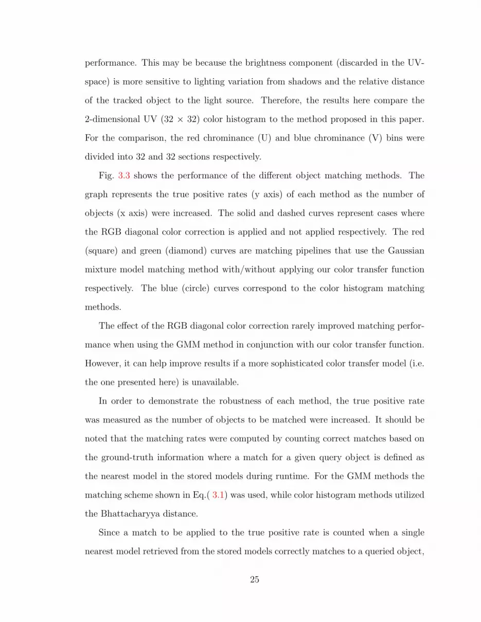
performance. This may be because the brightness component (discarded in the UV-

space) is more sensitive to lighting variation from shadows and the relative distance

of the tracked object to the light source. Therefore, the results here compare the

2-dimensional UV (32 × 32) color histogram to the method proposed in this paper.

For the comparison, the red chrominance (U) and blue chrominance (V) bins were

divided into 32 and 32 sections respectively.

Fig. 3.3 shows the performance of the different object matching methods. The

graph represents the true positive rates (y axis) of each method as the number of

objects (x axis) were increased. The solid and dashed curves represent cases where

the RGB diagonal color correction is applied and not applied respectively. The red

(square) and green (diamond) curves are matching pipelines that use the Gaussian

mixture model matching method with/without applying our color transfer function

respectively. The blue (circle) curves correspond to the color histogram matching

methods.

The effect of the RGB diagonal color correction rarely improved matching perfor-

mance when using the GMM method in conjunction with our color transfer function.

However, it can help improve results if a more sophisticated color transfer model (i.e.

the one presented here) is unavailable.

In order to demonstrate the robustness of each method, the true positive rate

was measured as the number of objects to be matched were increased. It should be

noted that the matching rates were computed by counting correct matches based on

the ground-truth information where a match for a given query object is defined as

the nearest model in the stored models during runtime. For the GMM methods the

matching scheme shown in Eq.( 3.1) was used, while color histogram methods utilized

the Bhattacharyya distance.

Since a match to be applied to the true positive rate is counted when a single

nearest model retrieved from the stored models correctly matches to a queried object,

25

Figure 3.3: Performance comparison of object different matching methods as com-pared to the approach introduced here. Graph shows the true positive rates (yaxis) versus the number of objects (x axis). The solid and dashed curves denotewith/without the RGB diagonal color correction (CC) respectively. CTF stands forthe color transfer function method.

it is not surprising that the true positive rates are decreasing relatively fast as the

number of objects are added in the model database. However, one would hope that a

recognition scheme that utilizes color transfer should still perform well as the number

of objects in the database becomes large.

It can be seen that matching methods using the color histogram showed better

performance when only the number of objects are small but as the number of increases

in the object model database the methods started breaking down. On the other hand,

the GMM methods using the color transfer function was resilient from the event of

increasing the number of objects. Quantitatively, the true positive rates of our method

was more than 11% higher than the more straightforward color histogram matching

methods, while average performance degradation rate of our method and the color

histogram were measured as 1.87% and 3.25% respectively. This means that the color

26

transfer method is almost half as affected from as a color histogram matching scheme

as the number of objects are increased.

Finally, we studied the separability of the objects in the database using the color

transfer measure and a the GMM matching scheme. Overall, the method should

be capable of reducing the appearance differences measured by similarity distance.

In order to measure this, the Φ distance between each object and itself across all

cameras was measured using the ground-truth object transition information provided

by the dataset. Fig. 3.4 plots the mean Φ distance computed for each object with

and without the color transfer.

Figure 3.4: The Φ error measure between each object and itself (based on ground-truth information) across all cameras with and without the color transfer function.


27

Chapter 4

Discussion

Most existing computational color constancy algorithms attempt to recover chro-

maticity information about the illumination in an input scene for which the only

known information is the sensor responses for each point (or color patch) in that

scene. In contrast to the color constancy work, our goal was to show how well the

color transfer method would do on an typical vision task, namely, consistent object

tracking in non-overlapping multi-camera video surveillance. In the multi-camera

video surveillance, the sensor response for point or patch is not generally known in

advance, rather it must be recovered by extracting pixels on the object as it moves

from one view to the next. Furthermore, change of object pose, size, and spectral

reflectance are likely as the object is observed in different cameras. These problems

make it nearly impossible to reliable correspond single color patches from the same

point on the object across views. We have shown that, instead of utilizing a color

calibration method that requires these correspondences, a more general model of color

transfer that relates the entire extracted color model in each view is feasible.

Due to the complexity of the problem and domain constraints, it is difficult to

directly compare the new approach to existing techniques that may require direct

pixel color correspondence. However, a few comments about similar methods and our

results can be made. In important and recent work, Javed et al. [29] have proposed

a brightness transfer function that is acquired across multiple non-overlapping views,

and run detailed experiments in three different multi-camera scenarios. The validity

of their subspace based method was demonstrated by using appearance combined with

supplements of known camera topology where the space-time information of entry and

exit locations, exit velocity and inter-camera time interval are available in prior. We

28

summarize their matching results of the three video scenarios for schemes they used.

The space-time scheme achieved a matching rate of 83%, 93% and 88%. When only

the brightness transfer function subspace was used, 88%, 90% and 81% were obtained.

As expected, the joint scheme showed the best results of 94%, 100% and 96%. These

performance results are similar to the ones achieved by the method proposed here.

However, the tracking schemes are quite different in that known camera topology

information was exploited in the maximum a posteriori estimation framework. This

can be a considerable advantage in order to increase the accuracies in tracking but is

quite constraining in a typical large-scale video surveillance network. However, it is

clear from the results that both the appearance and space-time models are important

sources of information as the tracking results improve significantly when both the

models are used jointly.

Other work [11] presents a novel solution to the inter-camera color calibration

problem, which is very important for multi-camera systems. This work considers

radiometric properties using a non-parametric function to model color distortion for

pair-wise camera combinations. A correlation matrix is computed from three 1-D

color histograms, and the model function is obtained from a minimum cost path

traced within the matrix. The first experiments was conducted with several synthe-

sized image pairs. Each pair consists of a reference image and a distorted version of its

illumination histogram. The histogram distortions were random, non-linear and non-

parametric. After the cross-correlation matrix and the model function are computed,

the histogram of the distorted image accordingly is transformed to obtained the illu-

mination corrected image. The improvement was substantial even though histogram

operations are invariant to spatial transformations but unfortunately the results were

not reported quantitatively. In a second experiment, images were acquired under dif-

ferent lighting conditions. Since each image was taken at a different time, there are

appearance mismatches in addition to the lighting and the camera difference. They

29

computed the aggregated cross-correlation matrices for each color channel from 150

pairs. It would be interesting to apply this technique to the challenging domain of

video surveillance and directly compare recognition rates (and degradation) to the

proposed approach. In particular, correlation between models (or histograms) must

to yield separability between objects in the database even as models are degraded.

There is a significant amount of work related to understanding the physics of

light change and determining how to predict and correct these changes. Much of

this work cannot be directly compared to our method because it requires point-wise

correspondence. However, some techniques utilize a diagonal transfer model[26, 12] of

illumination change that can be acquired under the same conditions as the work here.

The diagonal model simply describes the effect of moving from one scene illuminant to

another by scaling the R, G, and B channels via independent scale factors. These scale

factors can be written as the elements of a diagonal matrix. Previous work [20, 19] has

shown that the diagonal model works with the particular type of sensors which have

relatively narrow band and non-overlapping sensitivity functions under typical scene

illumination. One thus might claim that a simpler approach that relates RGB space

(as opposed to our UV approach) is linear and simple to compute. This is simply

not the case in the multi-camera video surveillance. As addressed factors above, it

is non-trivial to find corresponding pixel locations of the same object that will be

the cue to estimate the change in illumination. Moreover it is well known from the

illumination cone work of Belhumeur and Kriegman [27] to except for the case of a

planar object seen by a fixed camera and illuminated by point light sources at infinity,

RGB values of the object seen under different illuminations cannot be modeled by a

simple diagonal scaling.

The approach using a log chromaticity domain by Berwick and Lee [8] has the

advantage that it implies invariance under pure rotation. While we acknowledge if a

single cluster is centered at the origin this approach is useful, this work has shown

30

that object appearance in the UV space under different imaging conditions cannot be

modeled by a simple rotation. Rather, the appearance model of the object includes

multiple clusters as well as scaling. In this case, transformation to the log-polar

domain does not yield a rotational matching scheme.


31

Chapter 5

Conclusions and Future Work

In this work, a technique that estimates the unknown color transfer function between

pairs of disjoint cameras was introduced. Object appearance model correspondences,

generated as a subject moves throughout a surveillance network are provided as in-

put to a robust estimation procedure. Transfer functions are then able to predict

appearance change from one camera to the next and have been shown to increase

recognition capabilities of even simple object matching schemes to above 80% in an

indoor multi-camera network.

The technique was compared to a variety of baseline approaches of varying com-

plexity and was shown to outperform them. In particular, the technique degrades

more slowly than competing techniques as the number of objects to be matched

across views is increased. Although the method cannot be directly compared to sev-

eral state-of-the-art approaches in color calibration, either because these methods

require different operational conditions, or data is simply not available. Many of the

more related techniques were discussed in the context of our performance studies and

advantages and disadvantages of each technique was discussed.

5.1 Future Work

We have demonstrated the validity of the technique using color (rather than intensity)

to achieve matching stability of the recovered models. However, the method still relies

on several assumptions of varying complexity. Violation of these assumptions can lead

to degrade the robustness of the method. Future work as extensions to the current

method can be motivated by removing one or more of these assumptions.

Automatic detection and removal algorithms of self-shadows and non-isotropically

32

colored objects would be important in order to obtain more consistent appearance

models across difference camera views

Although we have emphasized the importance of using color to achieve stability

of the recovered models over time, changes in illuminate color, relative pose of the

cameras to the scene, or intrinsics, will require re-estimation of color transfer functions

online. (for example, sudden illumination changes caused by turning on and off lights,

adding lights, or clouds occluding sunlight). As future work, we are exploring online

incremental learning methods of the functions that will make this feasible.


33

Bibliography

[1] A.Dempster, N.Laird, and D.Rubin. Maximum-likelihood from incomplete datavia the em algorithm. J. Royal Statist. Soc. Series B 39, 1977.

[2] A.Elgammal, R.Duraiswami, D.Harwood, and L.Davis. Background and fore-ground modeling using nonparametric kernel density for visual surveillance. InProc. the IEEE, 2002.

[3] A.Mittal and L.Davis. Unified multi-camera detection and tracking using region-matching. In Proc. IEEE Workshop on Multi-Object Tracking, 2001.

[4] A.Rahimi, B.Dunagan, and T.Darrell. Simultaneous calibration and trackingwith a network of non-overlapping sensors. In Proc. Computer Vision and Pat-tern Recognition, volume 1, pages I–187– I–194, Jun 2004.

[5] C.Jaynes, A.Kale, N.Sanders, and E.Grossmann. The terrascope dataset: Ascripted multi-camera indoor video surveillance dataset with ground-truth. InProc. the IEEE Workshop on VS PETS, October 2005.

[6] C.Stauffer, W.Eric, and L.Grimson. Learning patterns of activity using real-timetracking. IEEE Trans. on Pattern Analysis and Machine Intelligence, 2000.

[7] C.Wren, A.Azarbayejani, T.Darrell, and A.Pentland. Pfinder: Real-time trackingof the human body. IEEE Trans. on Pattern Analysis and Machine Intelligence,1997.

[8] D.Berwick and S.Lee. A chromaticity space for specularity-, illumination color-and illumination pose-invariant 3-d object recognition. In ICCV, pages 165–170,1998.

[9] D.H.Johnson and G.Orsak. Relation of signal set choice to the performanceof optimal non-gaussian detectors. IEEE Trans. Comm., 41(9):1319–1328, Sep1993.

[10] F.M.Porikli and A.Divakaran. Multi-camera calibration, object tracking andquery generation. In Proc. IEEE International Conference on Multimedia andExpo (ICME), volume 1, pages 653–656, Jul 2003.

[11] F.Porikli. Inter-camera color calibration using cross-correlation model function.In Proc. IEEE Int. Conf. on Image Processing, 2003.

34

[12] G.D.Finlayson, B.Schiele, and J.L.Crowley. Comprehensive colour image nor-malization. In Proc. European Conference on Computer Vision, Jul 1998.

[13] Kideog Jeong and C.Jaynes. Object matching in disjoint cameras using a colortransfer approach. To Appear in Machine Vision and Applications Journal, 2006.

[14] J.Kang, I.Cohen, and G.Medioni. Persistent objects tracking across multiple nonoverlapping cameras. In Proc. IEEE wacv-motion 2005, volume 2 No.2, 2005.

[15] J.M.Speigle and D.H.Brainard. Predicting color from gray: The relationshipbetween achromatic adjustment and asymmetric matching. J. Opt. Soc. Am. A,16, No.10:2370–2376, Oct 1999.

[16] J.Orwell, P.Remagnino, and G.A.Jones. Multi-camera color tracking. In Proc.the Second IEEE Workshop on Visual Surveillance, 1999.

[17] J.S.Werner and B.E.Schefrin. Loci of achromatic points throughtout the lifespan. J. Opt. Soc. Am. A, 10, No.7:1509–1516, Jul 1993.

[18] J.Walraven and J.S.Werner. The invariance of unique white; a possible implica-tion for normalizing cone action spectra. Vision Res., 31:2185–2193, 1991.

[19] K.Barnard, L.Martin, A.Coath, and B.Funt. A comparison of color constancyalgorithms. part one: Methodology and experiments with synthesized data. IEEETransactions in Image Processing, 11(9):972–984, 2002.

[20] K.Barnard, V.Cardei, and B.Funt. A comparison of color constancy algorithms.part two: Experiments with image data. IEEE Transactions in Image Processing,11(9):985–996, 2002.

[21] K.Bauml. Color appearance: Effects of illuminant changes under different surfacecollections. J. Opt. Soc. Am. A, 11, No.2:531–542, Feb 1994.

[22] K.Jeong and C.Jaynes. Moving shadow detection using a combined geometricand color classification approach. In IEEE MOTION, 2005.

[23] M.D.Grossberg and S.K.Nayar. Determining the camera response from images:What is knowable? IEEE Transactions on Pattern Analysis and Machine Intel-ligence, 25(11):1455–1467, Nov 2003.

[24] M.Grossberg and S.K.Nayar. Modeling the space of camera response functions.IEEE Transactions on Pattern Analysis and Machine Intelligence, 26(10):1272–1282, Oct 2004.

[25] M.J.Swain and D.H.Ballard. Color indexing. International Journal of ComputerVision, 7:11–32, 1991.

[26] M.S.Drew, J.Wei, and Z.Li. Illumination-invariant color object recognition viacompressed chromaticity histograms of color-channel-normalized images. InComputer Vision, 1998. Sixth International Conference, pages 533–540, Jan1998.

35

[27] N.Belhumeur and D.Kriegman. What is the set of images of an object under allpossible illumination conditions? Int. Journal of Computer Vision, 28(3):245–260, 1998.

[28] N.Sanders and C.Jaynes. Class-specific color camera calibration with applicationto object recognition. In IEEE WACV, 2005.

[29] O.Javed, K.Shafique, and M.Shah. Appearance modeling for tracking in multiplenon-overlapping cameras. In Proc. IEEE International Conference on ComputerVision and Pattern Recognition (CVPR), pages 20–26, Jun 2005.

[30] P.J.Rousseeuw and A.M.Leroy. Robust Regression and Outlier Detection. JohnWiley and Sons, New York, 1987.

[31] Q.Xiong and C.Jaynes. Multi-resolution background modeling of dynamic scenesusing weighted match filters. In Proc. the ACM 2nd international workshop onVideo surveillance & sensor networks (VSSN ’04), pages 88–96, New York, NY,USA, 2004. ACM Press.

[32] R.Basri and D.W.Jacobs. Lambertian reflectance and linear subspaces. IEEETrans. on Pattern Analysis and Machine Intelligence, 25 no. 2:218–233, Feb 2003.

[33] R.Gross, J.Yang, and A.Waibel. Growing gaussian mixture models for poseinvariant face recognition. In Proc. the 15th International Conference on PatternRecognition, volume 1, pages 1088 – 1091, Sep 2000.

[34] Ying Shan, Harpreet S. Sawhney, and Rakesh Kumar. Vehicle identificationbetween non-overlapping cameras without direct feature matching. iccv, 1:378–385, 2005.

[35] Ying Shan, Harpreet S. Sawhney, and Rakesh (Teddy) Kumar. Unsupervisedlearning of discriminative edge measures for vehicle matching between non-overlapping cameras. cvpr, 1:894–901, 2005.

[36] S.Kullback and R.A.Leibler. On information and sufficiency. Annals of Mathe-matical Statistics, 22(1):79–86, March 1951.

[37] S.McKenna, Y.Raja, and S.Gong. Tracking colour objects using adaptive mixturemodels. Image and Vision Computing, pages 225–231, 1999.

[38] T.M.Cover and J.A.Thomas. Elements of Information Theory. Wiley, New York,1991.

36

VitaKideog Jeong

Background

• Date of Birth: February 28th, 1971

• Place of Birth: Busan (or Pusan), South Korea

Education

• Bachelor of Science in Computer Science, Chongju University, Chongju, SouthKorea, 1994

Professional Experience

• September 2004 - Present. Research Assistant, Metaverse Lab, Center for Vi-sualization and Virtual Environments.

• January 2003 - May 2004. Teaching Assistant, Department of Computer Sci-ence, University of Kentucky.

• January 1997 - June 2002. SAP R/3 Basis Engineer, TriGem Information Con-sulting, Inc.

• January 1994 - January 1997. Oracle Database Application Developer, TriGemComputer, Inc. (www.trigem.co.kr)

Publications

• K. Jeong and C. Jaynes, “Object Matching in Disjoint Cameras using a ColorTransfer Approach,” To Appear in Machine Vision and Applications Journal,2006, Springer Berlin Heidelberg, ISSN: 0932-8092

• K. Jeong and C. Jaynes, “Moving Shadow Detection using a Combined Geomet-ric and Color Classification Approach,” IEEE Workshop on Motion and VideoComputing (WACV/MOTION’05), Breckenridge, CO, January 5-7 2005.


37

object matching in disjoint cameras using a color transfer approach

Documents