nwt: towards natural audio-to-video generation with ... - arxiv
TRANSCRIPT

NWT: Towards natural audio-to-video generationwith representation learning
Rayhane MamaCash App Labs
Marc S. TyndelCash App Labs
Hashiam KadhimCash App Labs
Cole CliffordCash App Labs
Ragavan ThurairatnamCash App Labs
Abstract
In this work we introduce NWT, an expressive speech-to-video model. Unlikeapproaches that use domain-specific intermediate representations such as pose key-points, NWT learns its own latent representations, with minimal assumptions aboutthe audio and video content. To this end, we propose a novel discrete variationalautoencoder with adversarial loss, dVAE-Adv, which learns a new discrete latentrepresentation we call Memcodes. Memcodes are straightforward to implement,require no additional loss terms, are stable to train compared with other approaches,and show evidence of interpretability. To predict on the Memcode space, we usean autoregressive encoder-decoder model conditioned on audio. Additionally, ourmodel can control latent attributes in the generated video that are not annotated inthe data. We train NWT on clips from HBO’s Last Week Tonight with John Oliver.NWT consistently scores above other approaches in Mean Opinion Score (MOS) ontests of overall video naturalness, facial naturalness and expressiveness, and lipsyncquality. This work sets a strong baseline for generalized audio-to-video synthesis.Samples are available at https://next-week-tonight.github.io/NWT/.
1 Introduction
Video generation in deep learning is a challenging domain that lags behind other areas of syntheticmedia. Recent years have seen incredible generative modeling demonstrations in a variety of taskssuch as speech synthesis [20, 24], image generation [11, 44, 48], and natural language text generation[10]. While there have been interesting recent video synthesis works such as DVD-GAN [14], trainedon a diverse dataset to produce unconstrained video clips, video generation tasks with a specificgenerative goal have thus far mostly been accomplished in highly engineered or limited ways.
There are a number of existing approaches to generating video of a talking person from speechinput. To our knowledge, all previous approaches make use of either an engineered intermediaterepresentation such as pose keypoints, or real reference frames as part of the synthesis input, or both.
Speech2vid in 2017 was the first work to use raw audio data to generate a talking head, modifyingframes from a reference image or video [13]. Another work the same year called “SynthesizingObama” demonstrated substantially better perceptual quality, trained on a single subject [52]. It usesa network to predict lip shape, which is used to synthesize mouth shapes, which are recomposedinto video frames using reference frames. Another work, Neural Voice Puppetry aims to be quickly
Preprint. Under review.
arX
iv:2
106.
0428
3v1
[cs
.SD
] 8
Jun
202
1

adaptable to multiple subjects with a few minutes of additional video data [53]. It accomplishes this byusing a non-subject specific 3D face model as an intermediate representation, followed by a renderingnetwork that can be quickly tuned to produce subject-specific video. Published in 2020, Wav2Lip putsemphasis on being content-neutral; using reference frames it can produce compelling lipsync resultson unseen video [43]. This also allows it to include hand movement and body movement. Anotherapproach, Speech2Video (not to be confused with the similarly named Speech2vid mentioned above)uses pose as its intermediate representation and a labelled pose dictionary for each subject [37].
Engineered intermediate representations have the problem of constraining the output space. Thevideo rendering stage must make many assumptions from face keypoints, a representation with lowinformation content, in order to construct expressive motion. Small differences in facial expressioncan communicate highly significant expressive distinctions [41], resulting in important expressivevariations being represented with very little change in most intermediate representations of a face. Asa result, even if those differences are actually highly correlated with learned features from the audioinput, the video rendering stage must accomplish the difficult task of detecting them from a weaksignal.
Models that make use of reference frames, on the other hand, need manual selection of referencecontent in order for gestures and expression to match the audio. Most models that use referenceframes cannot know if, say, an eyebrow raise should not accompany a particular segment of speech.Speech2Video addresses this problem by allowing the model to select from a dictionary of labelledposes. This improves audio-video cohesion but requires extensive data preparation and results inexpressive range that can be limited by the scope of the reference dictionary.
Taking inspiration from recent advances in representation learning [5, 55], we took the approach ofseparating audio-to-video synthesis into two stages. Critically, unlike approaches that use engineeredspaces, we employ a fully learned intermediate representation, requiring minimal assumptions aboutwhat information is most important for reconstructing video. We train on one subject, John Oliver, butour data include clips spanning years of his show with noticeable variation in camera setup, lighting,clothing, hair, seating position, and age.
To accomplish this, we introduce the following contributions:
• a novel variational discrete autoencoder model, dVAE-Adv, including:
– a new discrete latent structure, Memcodes, whose elements are sampled from a combi-nation of multinomials.
– a training loss function for variational autoencoders (VAEs) that avoids averagingtendencies, or “blur”.
• an autoregressive sequence-to-sequence model that generates video from speech using theMemcode video space learned by the dVAE-Adv model.
Because NWT makes minimal assumptions about what should be captured in its intermediaterepresentation, it is capable of learning subtle expressive behaviors that might be lost in engineeredrepresentations. And because we do not use reference video frames as input, NWT renders full framesfrom scratch, meaning all gestures and motion are inferred from speech. NWT is also capable ofcontrolling labelled and unlabelled abstract properties of the output. The result1 is strikingly naturalfully synthesized video.
2 Method
Our approach aims to create a generalizable audio-to-video synthesis model that assumes little aboutthe content of either domain. Since autoregressive generative models have shown success in manydomains [10, 48, 54], we propose training an autoregressive video generator conditioned on eachclip’s corresponding audio. However, training such a model directly on pixels quickly results inscaling issues that constrain model size and video length. Additionally, autoregressive models trainedwith likelihood maximization on the pixel domain tend to dedicate a portion of their parameters tolearning high frequency details that are perceptually less important than low frequency structure.
1https://next-week-tonight.github.io/NWT/
2

(a) dVAE-Adv
(b) Prior autoregressive model
Figure 1: (a) dVAE-Adv architecture. The model creates a set of queries using its encoder, which doa lookup from a discrete embedding space (memory). The decoder builds its outputs from only theretrieved vectors. (b) Prior autoregressive model architecture. Dashed arrows denote sampling.
To address these two problems, we take inspiration from the representation learning ideas in VQ-VAE[55] and split our approach into two independently trained models:
• dVAE-Adv - A novel discrete variational autoencoder with an adversarial loss that com-presses video frames from 256 × 224 to a 16 × 14 latent space. We call each resultinglatent grid element a Memcode. Despite each Memcode carrying the information of about768 elements in the pixel domain, we do not see a significant perceptual degradation in thevisual quality of the reconstruction as shown in Section 3.6.
• Prior autogressive model - An encoder-decoder audio-to-video Memcode prediction modelthat autoregressively samples from the categorical distribution over the discrete representa-tion. Since this model operates on the Memcode space, memory requirements are low andthe network can avoid overspending parameters on high frequency artifacts.
Comparable approaches have been used in image [44, 45], audio [55], and video [57, 61] generation.
2.1 dVAE-Adv model
First, we train the dVAE-Adv model with a latent Memcode space of 16 × 14 video frames. Thismodel is trained on the video domain only, ignoring audio.
2.1.1 Attention as a multinomial discretization function
Sampling from a multinomial distribution is not differentiable, which prior works have addressedin a number of ways. Some approaches have used a Gumbel-softmax relaxation to graduallypush a softmax distribution towards a categorical one as temperature decreases [3, 23, 39]. Otherdiscretization schemes rely on a nearest neighbor selection coupled with a straight-through gradientestimator [6, 45, 55]. While Gumbel-softmax relaxation requires delicate tuning of temperatureannealing parameters, nearest neighbor selection requires the addition of both a vector quantizationobjective and a commitment loss.
We propose a new discretization technique with a gradient heuristic that learns a combination ofmultinomial distributions without requiring extra loss terms or tuning of temperature parameters.
We start by using the Gumbel-max trick to sample from a softmax distribution [30, 38]. The softmaxis defined by a vector of logits χ, over our model’s embedding codebook of size N :
α̃ = argmaxi∈{1,...,N}
(Smax (χ+G)) (1)
where G is the Gumbel noise and Smax is the softmax function.
Since argmax is not differentiable, we apply a straight-through gradient estimation. We find that thisapproximation works well in practice and is easy to implement in deep learning frameworks. Weprovide, in Algorithm 1, a simple gradient stopping trick to implement our trainable sampling.
Although we could write (1) without the softmax function, it is necessary during training to maintaingradient stability. The softmax can be omitted in inference.
3
In Appendix B.1.5, we justify our design choice to use the Gumbel-max trick over performing naturalsampling from the softmax distribution coupled with a straight-through gradient estimation.
We compute the log-probabilities χ as a content-based similarity measure between the encoder’soutputs and the model’s latent codebook. We base this similarity metric on the scaled dot-productattention where the queries Q are the projected encoder’s outputs, and the keys K and values V arelinear projections of the discrete codebook [56].
We thus define our entire discretization layer as:
HardAttn(Q,K, V ) = eα̃V (2)
α̃ = argmaxi∈{1,...,N}
(α) ; α = Smax
(QKT
√dK
+G
)(3)
where eα̃ is the standard basis vector in RN (one hot encoding of α̃).
Since we want each code to consist of multiple multinomial samples, we use multi-headed attentionin our discretization layer [56]. This yields three benefits over a single softmax distribution:
• The structure enables Nh permutations per Memcode where h is the number of heads,allowing a large discrete space using a small codebook size.
• Similar to multivariate Gaussian latents with a diagonal covariance matrix, multi-headmultinomial sampling can learn interpretable high level representations of inputs (see A.1).
• It enables a distance measure between Memcode values, and we find the Hamming distanceto be well correlated with loss (see A.2).
2.1.2 Learning
We start by defining the objective of dVAE-Adv as minimizing the negative evidence lower bound(ELBO) of the marginal likelihood of the data [18, 28]:
LELBO(x) = Ez∼qφ(z|x)
[− log pθ(x|z)] + βDKL(qφ(z|x)||p(z)) (4)
− log p(x) ≤ LELBO(x) (5)
where qφ(z|x) and pθ(x|z) denote the variational encoder and decoder respectively. β is the KL-annealing loss weight that we find important to tune on video data [8], although ELBO is only definedfor β = 1.
In practice, training VAEs to minimize the negative ELBO alone typically yields models that predictaverages over high-frequency details of data. This tendency results in blurry output images forimage generation tasks [21, 44], overly smoothed videos for video generation tasks [62], and muffledaudio for audio generation tasks [33]. Autoregressive decoders have been used to mitigate this issue[12], but predicting outputs one element at a time is slow, especially in the video domain. Anotherapproach, inverse autoregressive flows, requires very deep models and an intricate training setup [29].
To overcome the high frequency averaging problem, we propose training dVAE-Adv with the additionof a Wasserstein adversarial loss term [2]. Letting Dc be critic c of C from the set of critics Sc, wedefine the adversarial loss of dVAE-Adv as:
Lgan =∑c∈SC
Ez∼qφ(z|x)
[−Dc(pθ(x|z))] (6)
Additionally, we replace the expected negative log likelihood from (4) with a reconstruction errorexpressed inside the critics, in a similar way to Larsen et al. [35]:
Lrecon =∑c∈SC
∑l∈SLc
Ez∼qφ(z|x)
[− log pθ(D
lc(x)|z)
](7)
4
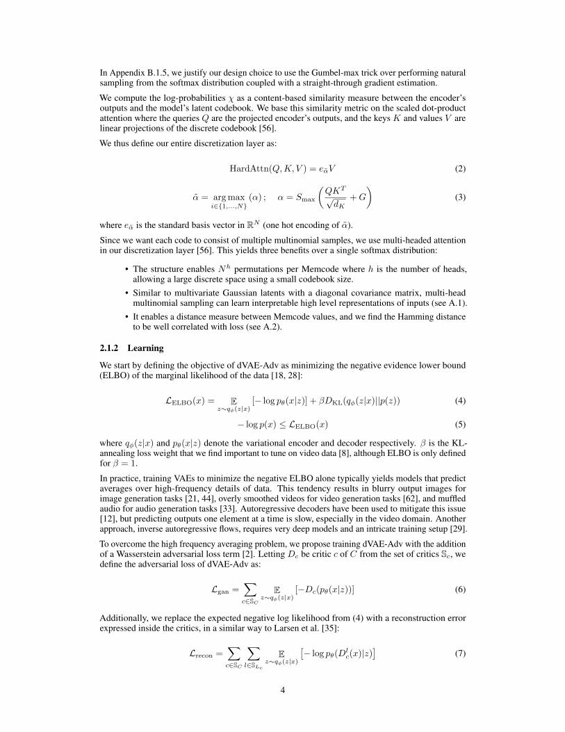
Algorithm 1 Differentiable multinomial sampling
Input: A vector of logits χ, a softmax function Smax, a uniform distribution U , a onehot functiononehot, an argmax function argmax, a stop gradient function SGOutput: vector of one-hot weights α̃u ∼ U(0, 1)G← − log(− log(u))α← Smax(χ+G)α̃← onehot(argmax(α))α̃← SG(α̃− α) + α
where Dlc(x) denotes the hidden representation of the lth layer of critic c from the set of layers SLc
of size Lc for critic c. This minimizes the feature matching loss between the critics’ feature mapsfor the targets and generator outputs [33]. It is also similar to Hou et al. [19], but does not require apretrained VGGNet to compute the feature maps [50].
We evaluate our reconstruction loss under the Laplace distribution resulting in a simple L1 lossand we assume the prior p(z) to be uniform over the latent categories. We train all of dVAE-Adv’sgenerator model parameters (θ and φ) with the final loss function:
Lgen = Lrecon + γLgan + βDKL (qφ(z|x)||p(z)) (8)
where γ is used to weight the contribution of the adversarial loss compared to the reconstruction loss.
Finally, we train our set of critics on the improved Wasserstein GAN loss [16]:
Ladv =∑c∈SC
(E
z∼qφ(z|x)[Dc(pθ(x|z))]− E
x∼Pr[Dc(x)] + λ E
x̂∼Px̂
[(‖∇x̂Dc(x̂)‖2 − 1)
2])
(9)
where x̂ is sampled uniformly along straight lines between real samples from data distribution Pr andgenerated samples from generator distribution pθ(x|z). We implicitly define this distribution as Px̂.We present an overview of the training procedure in Appendix C.1.
Our approach is similar to VAE-GAN [35], but VAE-GAN does an additional decoding step on zp,sampled from prior p(z). There, the goal is generating realistic video from the uniform prior. Thisslows down training and is unnecessary for our task since we are not looking to sample from p(z).
Furthermore, training the decoder on samples from the prior encourages it to generate videos thatfool the critics, but not necessarily faithfully reconstruct the input videos [35]. We expect that thiswould adversely impact lipsync performance in our downstream task and we found the realism versusreconstruction trade-off to be fully controllable by γ without the need for an extra decoding step.
2.1.3 Architecture
Figure 1a depicts an overview of the dVAE-Adv architecture. The encoder starts with spatialdownsampling of the frames independently, followed by temporal feature extraction, whose outputsquery a multi-headed hard attention block. The attention block outputs become the inputs to thedecoder, which is a mirror of the encoder, using 2D nearest neighbour upsampling. dVAE-Adv alsoincludes critic models with different parameters, including 3D models (temporal coherence) and 2Dmodels (independent frame quality). A detailed explanation of the dVAE-Adv architecture can befound in Appendix B.1.
2.1.4 Attention as a memory-augmentation
dVAE-Adv can be viewed as a memory-augmented network [15] where the embedding codebook isa trainable external memory table that stores key information about the data. During training, themodel extracts and memorizes key data features. During inference, the input data guides the memorylookup from the embedding table. It is possible to frame our work as a special case of van den Oordet al. [55] where the similarity metric is learnable instead of nearest neighbors. Our model is also a
5
special case of Lample et al. [34], Wang et al. [58] where our memory read is discrete, resulting inour attention heads learning more separable characteristics about the inputs (see Appendix A.1).
2.2 Prior autoregressive model
In this section, we train an autoregressive conditional model pψ(z|y) to generate video Memcodesfrom audio y (Figure 1b). We freeze the dVAE-Adv model’s weights in order to train the priorautoregressive model. Throughout this work, we use Mel spectrograms as our audio representation[49], a common approach in speech-related learning tasks, but other audio representations shouldalso work.
2.2.1 Learning
To create video Memcode targets for the prior autoregressive model, we sample once from themultinomial modeled by the dVAE-Adv encoder qφ(z|x) for each clip 2. As the number of samplesgrows, this becomes equivalent to using the softmax distribution probabilities as soft targets.
The prior autoregressive model is trained in a supervised fashion to minimize the KL divergencebetween qφ(z|x) and pψ(z|y). Since all of dVAE-Adv’s parameters are frozen during this phase andthe latent targets z are only sampled once, minimizing the KL divergence is equivalent to minimizingthe cross entropy between z and the prior model’s predictions.
2.2.2 Architecture
We suggest training prior models with two different autoregressive strategies:
• Frame level AR (FAR): Autoregressively predict video frames, one frame at a time. Themodel makes 16× 14× h predictions each decoding step. This mix of autoregressive andparallel behaviour enables real time inference speed on GPUs.
• Memcode level AR (MAR): Autoregressively predict one element of the Memcode videoframe at a time. The model makes h predictions on every decoding step. This model can beperceived as a fully AR model from the perspective of predicting one image patch at a time.
A third strategy, head level AR (HAR), meaning autoregressively predicting each head of eachMemcode (one prediction per step) is computationally slow and we did not explore it at this time.
All of these models are convolutional [32] encoder-decoder models. Despite their successes in otherdomains [10, 44, 56, 61], we hypothesize that transformers would not provide substantial benefitin our case: transformers excel at learning long term relationships but need more memory to do so,which is not ideal under our hardware constraints.
The architecture (Figure 1b) consists of three components: an audio encoder that analyses audiospectrogram inputs, a video decoder which autoregressively predicts elements one by one (frames forFAR, Memcodes for MAR), and a variational latent encoder that creates a highly compressed, fixedsize, multivariate Gaussian latent style representation zl of the target Memcodes. The latent encoderenables the model to learn characteristics of the target that are poorly correlated with the audio input.Appendix B.2 contains a more detailed explanation of the architecture and latent style representation.
3 Experiments and results
3.1 Dataset
Our dataset consists of cleaned video samples of Last Week Tonight with John Oliver (LWT). Thetotal dataset consists of 33.4 hours of video, collected from 215 episodes and split into 16127 videoclips of an average length 7.46 seconds, interpolated to 30 FPS. See Appendix D for more detailsincluding the collection and cleaning process.
2We found sampling from qφ(z|x) yielded more dynamic results than simply picking the argmax.
6

Table 1: Mean Opinion Score (MOS) evaluations with 95% confidence intervals computed from thet-distribution. NWT X Samp stands for style sampling on X type model, while NWT X CONDstands for style copying on X type model (style sampling and copying explained in Section 3.5)
Model Overall Naturalness Face Naturalness Lipsync Accuracy
Talking Face – 1.419± 0.052 –Wav2Lip + GAN – – 2.058± 0.070
NWT FAR Samp 2.402± 0.077 3.570± 0.090 3.662± 0.074NWT FAR Cond 2.481± 0.079 3.622± 0.087 3.666± 0.076NWT MAR Samp 2.835± 0.075 3.915± 0.079 3.872± 0.071NWT MAR Cond 2.837± 0.078 3.960± 0.079 3.883± 0.068
Ground Truth 4.798± 0.026 4.802± 0.027 4.787± 0.023
3.2 Model details
Among related previous work in talking human video generation, only LumièreNet [25] andSpeech2Video [37] generate all pixels of the output video without any reference frames as in-put. However, LumièreNet uses body heatmaps that omit intra-facial information, and Speech2Videorequires a large human-labelled dictionary of reference poses mapped to vocabulary, which we do nothave for our data. Since these issues prevent us from performing direct comparisons using the samedata, we compare our general audio-to-video model with two models for specific tasks: Wav2Lip[43] and “Audio-driven Talking Face Video Generation” [64] which we refer to as Talking Face. Forfairness, we design separate metrics when comparing each of these models, explained in 3.3.
We train dVAE-Adv with Adam optimizer [27] for 150, 000 steps with a batch size of 16 videos eachcontaining 30 frames distributed across 16 NVIDIA A100 40GB GPUs. We found that the model isable to generate arbitrary video length without quality decay during inference. More details and thedVAE-Adv model parameters are in Appendix C.2.1
We train our prior autoregressive models with Adam optimizer for 250, 000 steps with a batch size of64 distributed across 8 NVIDIA A100 GPUs. Each sample is limited to 32 frames during training.For a more detailed description including model parameters, see Appendix C.2.2.
For the Talking Face model, we fine-tune the memory-augmented GAN version of Talking Face asinstructed in its documentation on our LWT dataset. We use training and inference parameters asrecommended in the authors’ codebase. To avoid discrepancy between the training and inferencedistributions, we ensure the reference videos and test audio are sourced from the same episode.
For the Wav2Lip model, we tried both the zero-shot approach using pre-trained models and trainingfrom scratch on our dataset, and found the former, specifically the pre-trained model with an adversary,was better. Similarly to Talking Face, we select a random training sample from the same episode asthe test audio input to use as the reference input.
3.3 Evaluation
We conducted three separate subjective mean opinion score (MOS) experiments. In the first ex-periment, participants were instructed to rate the overall naturalness of the generated clip; in thesecond, to specifically rate the face’s naturalness and expressiveness; and in the third, to rate thenaturalness and accuracy of the lipsync. The bottom half of videos were removed for the latter two sothat participants focus on the face and mouth. Table 1 shows comparisons between our models andrelevant baselines. In the first experiment, we compare NWT with ground truth videos. In the second,we compare NWT with Talking Face [64] and the ground truth videos. In the last experiment, wecompare NWT with Wav2Lip + GAN [43], as well as ground truth videos. Details about our MOSsetup are in Appendix E.
As seen in Table 1, our end-to-end models, which are not explicitly trained for the lipsync task,outperform the Wav2Lip + GAN lipsync model. By manually inspecting generated samples fromboth models, we find that NWT generates more natural and smooth mouth movements. Wav2Lip +
7
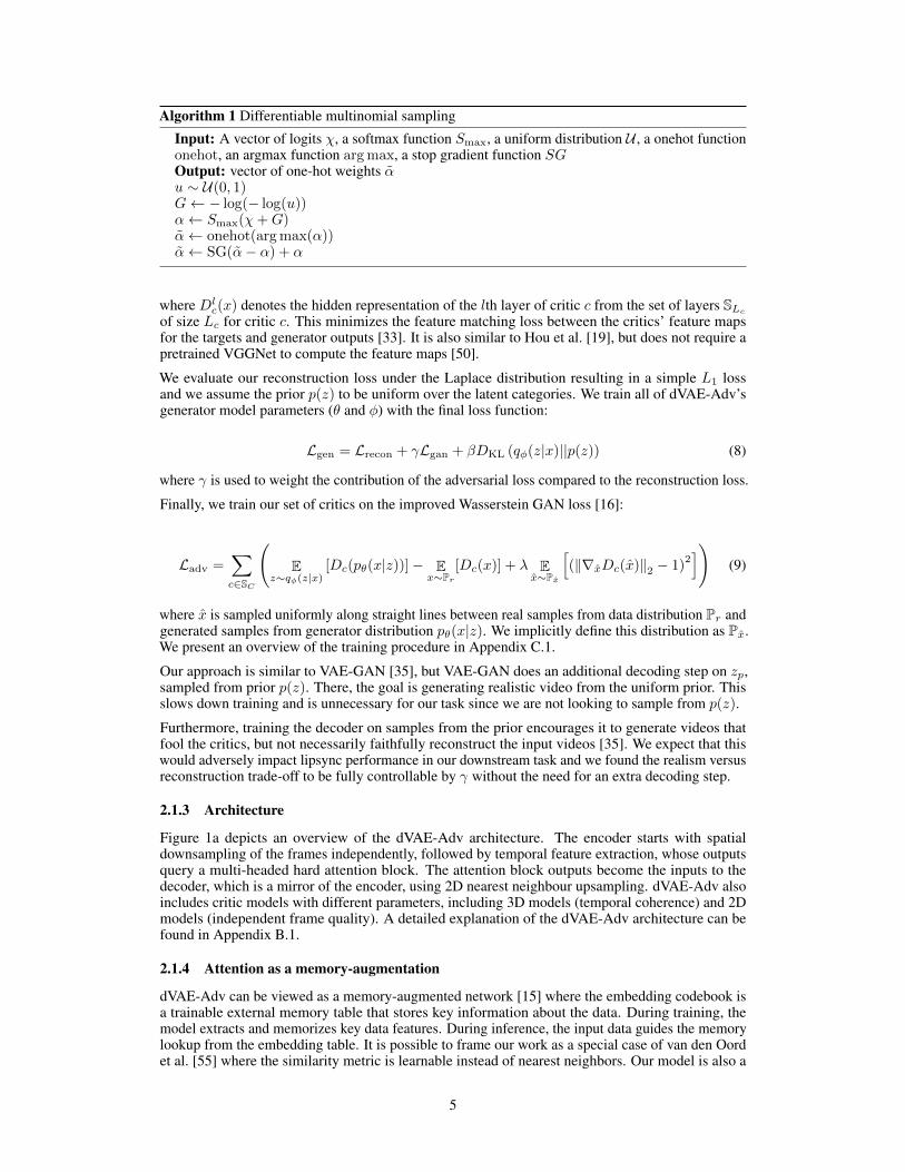
Table 2: Compression rate comparison of different video compression systems on our test data usingstructural similarity index measure (SSIM) [59]. The Mem16 model has a latent space of 16× 14and the Mem8 model has a latent space of 8× 7. Each Memcode contains 24 bits of information.
Model Data size (GB) Relative compression to h264 Frame SSIM
h264 0.289 1× 0.9452
dVAE-Adv Mem16 0.223 1.30× 0.9499dVAE-Adv Mem16 + RLE 0.146 1.98× 0.9499dVAE-Adv Mem8 0.112 2.58× 0.9412dVAE-Adv Mem8 + RLE 0.072 4.01× 0.9412
Uncompressed 57.83 – 1.0
GAN’s quality can drop when there is greater movement of the subject’s head in the reference video,and from time to time the mouth detection fails resulting in bad outputs. NWT does not suffer fromthese issues since the full video is generated from scratch.
NWT also significantly outperforms the Talking Face model, which struggles to correctly render anatural face on volatile reference heads. In contrast, our method generates a large variety of facialexpressions that pair naturally with the input audio. We demonstrate in Samples Section S1 that NWTgenerates facial expressions and body language that are tightly connected to tone of speech.
The overall naturalness MOS experiment shows that, despite our model being a strong baseline fornatural human audio-to-video generation, there is still a sizable gap between real videos and ourmodel. This is likely due to NWT’s shortcomings in rendering Oliver’s hands and gestures. Ourinterpretation of this limitation is that Oliver has a wide variety of gestures that have relatively weakercorrelations with speech audio features (compared to lip position and head movement), and the datasize is too small to learn this well. We expect our model would perform better in this regard if trainedon less emotive and dynamic subjects than John Oliver.
Finally, MAR models perform better than FAR models in terms of MOS, which is likely due to theadditional stability that MAR models have over FAR. We show quality comparisons of generatedvideos from these models in samples section S4 and we show the training and inference speeds ofeach model in Appendix C.3.
3.4 Episode control
As the data contain 215 episodes varying in camera setup, lighting, clothing, hair, position, and age,we propose a hierarchical episode embedding for both dVAE-Adv and the prior autoregressive model,similar to speaker embeddings in multi-speaker text-to-speech models [51, 54] (Appendix B.3).
We show in Samples Section S2 that we can generate video clips from different episodes given thesame audio input. In these examples, the episode embedding of dVAE-Adv alone mainly changesglobal color filters, while the combination of episode embeddings from both models perform acomplete episode translation. We hypothesize this behaviour would generalize to multi-actor datasets.
3.5 Style control
In this section, we examine the properties of the unsupervisedly learned style latent representationszl, and demonstrate how they control features that weakly depend on audio (Samples Section S3).
To understand the effect of the style latent vectors, we randomly sampled an initial vector from theprior p(zl). We then manually change one variate from the latent vector and analyze the results. Weshow that some variates control human-interpretable features, such as camera angles or the presenceof side overlay boxes from the show.
We further demonstrate that we can provide an optional video reference input xr to the model toguide the style of the output video. We sample zl from the posterior q(zl|zr) where zr is sampledfrom the posterior qφ(zr|xr) (see B.2). We show that, for an audio input that is different from theaudio of the reference xr, the model copies relevant abstract traits from xr in the generated sample.
8

3.6 Video Compression
A byproduct of this work is neural video compression. Memcodes act as an efficient representationof video data that lies within the distribution of the training data. In Table 2 we compare dVAE-Advmodels with two downsampling rates to the more general industry standard compression algorithmh264 [60] applied on our test set. We find that dVAE-Adv models can achieve higher compressionrates than h264 for comparable reconstruction quality measured by mean frame SSIM [59].
With argmax sampling, we find that most Memcode heads tend not to change between adjacentframes. We can therefore use a lossless run length encoding (RLE) on the latent video representations.dVAE-Adv + RLE models achieve 2× and 4× more compression relative to h264 respectively for16× 14 and 8× 7 latent space dimensions. Both models exhibit comparable SSIM metrics. We showperceptual comparisons of these compression methods in section S5.
4 Applications and broader impact
There are countless exciting applications to flexible video synthesis. It could provide ways to createhyper-realistic show hosts who can be localised to different languages. It presents a new approachto generating dynamic human-like characters in video games. If this approach can be extended toperform a language translation task, it provides a path towards automated sign language interpreting.
However, like many emerging technologies, there are potential nefarious uses that warrant seriousattention. Synthetic media can enable the creation of content deliberately designed to mislead ordeceive. Risk mitigation work has mostly been in synthetic media detection [1, 7, 47]. While NWT ismore general than face swapping or lipsync techniques, we believe similar detection approaches canprove effective and that it is important for research to take place while these technologies are new.
5 Future work
A clear subsequent direction for NWT is training larger models on much bigger datasets consisting ofmany subjects. The ability of our model to handle the diverse varieties of individual subjects suggeststhis flexibility is likely possible. Another idea to explore is replacing the episode embedding with acloning component, enabling the model to mimic a particular episode given a frame or partial image.This could further be extended to models that can imitate speakers or contexts unseen during training.
It would also be interesting to apply our techniques to non-video domains, such as audio generationor image generation tasks. We would also like to explore disentanglement between Memcode heads,or ideas such as hierarchical Memcodes.
6 Conclusion
We describe NWT, a new approach for synthesizing realistic, expressive video from audio. Weintroduced a new discrete autoencoder, dVAE-Adv, highlighting the multi-headed structure of itslatent space which we term Memcodes. We showed that this approach, which avoids implicitbias regarding the contents of video or audio in its architecture, significantly outperforms previousspecialized approaches to lipsync and face generation tasks in subjective evaluation tests, while alsoclustering many latent features without supervision. We evaluated our model on several generationcontrol tasks, demonstrating that we can vary episodes and recording setup independently fromspeech. Our model would also be easy to link to existing text-to-speech models, which would enableend-to-end text-to-video generation.
Our work sets a new standard for expressiveness in talking human video synthesis and shows potentialfor more general applications in the future.
Acknowledgments and Disclosure of Funding
The authors would like to thank Alex Krizhevsky for his mentorship and insightful discussions. Theauthors also thank Alyssa Kuhnert, Aydin Polat, Joe Palermo, Pippin Lee, Stephen Piron, and VinceWong for feedback and support.
9
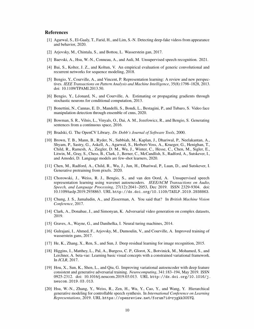
References[1] Agarwal, S., El-Gaaly, T., Farid, H., and Lim, S.-N. Detecting deep-fake videos from appearance
and behavior, 2020.
[2] Arjovsky, M., Chintala, S., and Bottou, L. Wasserstein gan, 2017.
[3] Baevski, A., Hsu, W.-N., Conneau, A., and Auli, M. Unsupervised speech recognition. 2021.
[4] Bai, S., Kolter, J. Z., and Koltun, V. An empirical evaluation of generic convolutional andrecurrent networks for sequence modeling, 2018.
[5] Bengio, Y., Courville, A., and Vincent, P. Representation learning: A review and new perspec-tives. IEEE Transactions on Pattern Analysis and Machine Intelligence, 35(8):1798–1828, 2013.doi: 10.1109/TPAMI.2013.50.
[6] Bengio, Y., Léonard, N., and Courville, A. Estimating or propagating gradients throughstochastic neurons for conditional computation, 2013.
[7] Bonettini, N., Cannas, E. D., Mandelli, S., Bondi, L., Bestagini, P., and Tubaro, S. Video facemanipulation detection through ensemble of cnns, 2020.
[8] Bowman, S. R., Vilnis, L., Vinyals, O., Dai, A. M., Jozefowicz, R., and Bengio, S. Generatingsentences from a continuous space, 2016.
[9] Bradski, G. The OpenCV Library. Dr. Dobb’s Journal of Software Tools, 2000.
[10] Brown, T. B., Mann, B., Ryder, N., Subbiah, M., Kaplan, J., Dhariwal, P., Neelakantan, A.,Shyam, P., Sastry, G., Askell, A., Agarwal, S., Herbert-Voss, A., Krueger, G., Henighan, T.,Child, R., Ramesh, A., Ziegler, D. M., Wu, J., Winter, C., Hesse, C., Chen, M., Sigler, E.,Litwin, M., Gray, S., Chess, B., Clark, J., Berner, C., McCandlish, S., Radford, A., Sutskever, I.,and Amodei, D. Language models are few-shot learners, 2020.
[11] Chen, M., Radford, A., Child, R., Wu, J., Jun, H., Dhariwal, P., Luan, D., and Sutskever, I.Generative pretraining from pixels. 2020.
[12] Chorowski, J., Weiss, R. J., Bengio, S., and van den Oord, A. Unsupervised speechrepresentation learning using wavenet autoencoders. IEEE/ACM Transactions on Audio,Speech, and Language Processing, 27(12):2041–2053, Dec 2019. ISSN 2329-9304. doi:10.1109/taslp.2019.2938863. URL http://dx.doi.org/10.1109/TASLP.2019.2938863.
[13] Chung, J. S., Jamaludin, A., and Zisserman, A. You said that? In British Machine VisionConference, 2017.
[14] Clark, A., Donahue, J., and Simonyan, K. Adversarial video generation on complex datasets,2019.
[15] Graves, A., Wayne, G., and Danihelka, I. Neural turing machines, 2014.
[16] Gulrajani, I., Ahmed, F., Arjovsky, M., Dumoulin, V., and Courville, A. Improved training ofwasserstein gans, 2017.
[17] He, K., Zhang, X., Ren, S., and Sun, J. Deep residual learning for image recognition, 2015.
[18] Higgins, I., Matthey, L., Pal, A., Burgess, C. P., Glorot, X., Botvinick, M., Mohamed, S., andLerchner, A. beta-vae: Learning basic visual concepts with a constrained variational framework.In ICLR, 2017.
[19] Hou, X., Sun, K., Shen, L., and Qiu, G. Improving variational autoencoder with deep featureconsistent and generative adversarial training. Neurocomputing, 341:183–194, May 2019. ISSN0925-2312. doi: 10.1016/j.neucom.2019.03.013. URL http://dx.doi.org/10.1016/j.neucom.2019.03.013.
[20] Hsu, W.-N., Zhang, Y., Weiss, R., Zen, H., Wu, Y., Cao, Y., and Wang, Y. Hierarchicalgenerative modeling for controllable speech synthesis. In International Conference on LearningRepresentations, 2019. URL https://openreview.net/forum?id=rygkk305YQ.
10

[21] Huang, H., li, z., He, R., Sun, Z., and Tan, T. Introvae: Introspective variational autoencodersfor photographic image synthesis. In Bengio, S., Wallach, H., Larochelle, H., Grauman,K., Cesa-Bianchi, N., and Garnett, R. (eds.), Advances in Neural Information ProcessingSystems, volume 31. Curran Associates, Inc., 2018. URL https://proceedings.neurips.cc/paper/2018/file/093f65e080a295f8076b1c5722a46aa2-Paper.pdf.
[22] Isola, P., Zhu, J.-Y., Zhou, T., and Efros, A. A. Image-to-image translation with conditionaladversarial networks, 2018.
[23] Jang, E., Gu, S., and Poole, B. Categorical reparameterization with gumbel-softmax, 2017.
[24] Jia, Y., Zen, H., Shen, J., Zhang, Y., and Wu, Y. Png BERT: augmented BERT on phonemesand graphemes for neural TTS. CoRR, abs/2103.15060, 2021. URL https://arxiv.org/abs/2103.15060.
[25] Kim, B. and Ganapathi, V. Lumièrenet: Lecture video synthesis from audio. CoRR,abs/1907.02253, 2019. URL http://arxiv.org/abs/1907.02253.
[26] Kim, Y., Wiseman, S., Miller, A. C., Sontag, D., and Rush, A. M. Semi-amortized variationalautoencoders, 2018.
[27] Kingma, D. P. and Ba, J. Adam: A method for stochastic optimization. In Bengio, Y. andLeCun, Y. (eds.), 3rd International Conference on Learning Representations, ICLR 2015,San Diego, CA, USA, May 7-9, 2015, Conference Track Proceedings, 2015. URL http://arxiv.org/abs/1412.6980.
[28] Kingma, D. P. and Welling, M. Auto-encoding variational bayes. In 2nd International Con-ference on Learning Representations, ICLR 2014, Banff, AB, Canada, April 14-16, 2014,Conference Track Proceedings, 2014.
[29] Kingma, D. P., Salimans, T., Jozefowicz, R., Chen, X., Sutskever, I., and Welling, M. Improvingvariational inference with inverse autoregressive flow, 2017.
[30] Kool, W., van Hoof, H., and Welling, M. Stochastic beams and where to find them: Thegumbel-top-k trick for sampling sequences without replacement, 2019.
[31] Krizhevsky, A. and Hinton, G. E. Using very deep autoencoders for content-based image re-trieval. In ESANN, 2011. URL http://dblp.uni-trier.de/db/conf/esann/esann2011.html#KrizhevskyH11.
[32] Krizhevsky, A., Sutskever, I., and Hinton, G. E. Imagenet classification with deep con-volutional neural networks. In Pereira, F., Burges, C. J. C., Bottou, L., and Weinberger,K. Q. (eds.), Advances in Neural Information Processing Systems, volume 25. CurranAssociates, Inc., 2012. URL https://proceedings.neurips.cc/paper/2012/file/c399862d3b9d6b76c8436e924a68c45b-Paper.pdf.
[33] Kumar, K., Kumar, R., de Boissiere, T., Gestin, L., Teoh, W. Z., Sotelo, J., de Brebisson,A., Bengio, Y., and Courville, A. Melgan: Generative adversarial networks for conditionalwaveform synthesis, 2019.
[34] Lample, G., Sablayrolles, A., Ranzato, M., Denoyer, L., and Jégou, H. Large memory layerswith product keys, 2019.
[35] Larsen, A. B. L., Sønderby, S. K., Larochelle, H., and Winther, O. Autoencoding beyond pixelsusing a learned similarity metric, 2016.
[36] LeCun, Y. and Cortes, C. MNIST handwritten digit database. 2010. URL http://yann.lecun.com/exdb/mnist/.
[37] Liao, M., Zhang, S., Wang, P., Zhu, H., Zuo, X., and Yang, R. Speech2video synthesis with 3dskeleton regularization and expressive body poses, 2020.
[38] Maddison, C. J., Tarlow, D., and Minka, T. A∗ sampling. In Ghahramani, Z., Welling, M.,Cortes, C., Lawrence, N., and Weinberger, K. Q. (eds.), Advances in Neural InformationProcessing Systems, volume 27. Curran Associates, Inc., 2014.
11
[39] Maddison, C. J., Mnih, A., and Teh, Y. W. The concrete distribution: A continuous relaxationof discrete random variables, 2017.
[40] Odena, A., Dumoulin, V., and Olah, C. Deconvolution and checkerboard artifacts. Distill, 2016.doi: 10.23915/distill.00003. URL http://distill.pub/2016/deconv-checkerboard.
[41] Olszanowski, M., Pochwatko, G., Kuklinski, K., Scibor-Rylski, M., Lewinski, P., and Ohme,R. K. Warsaw set of emotional facial expression pictures: a validation study of facial displayphotographs. Frontiers in Psychology, 5:1516, 2015. ISSN 1664-1078. doi: 10.3389/fpsyg.2014.01516. URL https://www.frontiersin.org/article/10.3389/fpsyg.2014.01516.
[42] Paine, T. L., Khorrami, P., Chang, S., Zhang, Y., Ramachandran, P., Hasegawa-Johnson, M. A.,and Huang, T. S. Fast wavenet generation algorithm, 2016.
[43] Prajwal, K. R., Mukhopadhyay, R., Namboodiri, V. P., and Jawahar, C. A lip sync expert is allyou need for speech to lip generation in the wild. Proceedings of the 28th ACM InternationalConference on Multimedia, Oct 2020. doi: 10.1145/3394171.3413532. URL http://dx.doi.org/10.1145/3394171.3413532.
[44] Ramesh, A., Pavlov, M., Goh, G., Gray, S., Voss, C., Radford, A., Chen, M., and Sutskever, I.Zero-shot text-to-image generation, 2021.
[45] Razavi, A., van den Oord, A., and Vinyals, O. Generating diverse high-fidelity images withvq-vae-2, 2019.
[46] Ribeiro, F., Florêncio, D., Zhang, C., and Seltzer, M. Crowdmos: An approach for crowdsourc-ing mean opinion score studies. In 2011 IEEE International Conference on Acoustics, Speechand Signal Processing (ICASSP), pp. 2416–2419, 2011. doi: 10.1109/ICASSP.2011.5946971.
[47] Rössler, A., Cozzolino, D., Verdoliva, L., Riess, C., Thies, J., and Nießner, M. Faceforensics++:Learning to detect manipulated facial images, 2019.
[48] Salimans, T., Karpathy, A., Chen, X., and Kingma, D. P. Pixelcnn++: Improving the pixelcnnwith discretized logistic mixture likelihood and other modifications, 2017.
[49] Shen, J., Pang, R., Weiss, R. J., Schuster, M., Jaitly, N., Yang, Z., Chen, Z., Zhang, Y., Wang, Y.,Skerry-Ryan, R., Saurous, R. A., Agiomyrgiannakis, Y., and Wu, Y. Natural tts synthesis byconditioning wavenet on mel spectrogram predictions, 2018.
[50] Simonyan, K. and Zisserman, A. Very deep convolutional networks for large-scale imagerecognition, 2015.
[51] Skerry-Ryan, R., Battenberg, E., Xiao, Y., Wang, Y., Stanton, D., Shor, J., Weiss, R. J., Clark,R., and Saurous, R. A. Towards end-to-end prosody transfer for expressive speech synthesiswith tacotron, 2018.
[52] Suwajanakorn, S., Seitz, S. M., and Kemelmacher-Shlizerman, I. Synthesizing obama: Learninglip sync from audio. ACM Trans. Graph., 36(4), July 2017. ISSN 0730-0301. doi: 10.1145/3072959.3073640. URL https://doi.org/10.1145/3072959.3073640.
[53] Thies, J., Elgharib, M. A., Tewari, A., Theobalt, C., and Nießner, M. Neural voice puppetry:Audio-driven facial reenactment. In ECCV, 2020.
[54] van den Oord, A., Dieleman, S., Zen, H., Simonyan, K., Vinyals, O., Graves, A., Kalchbrenner,N., Senior, A., and Kavukcuoglu, K. Wavenet: A generative model for raw audio, 2016.
[55] van den Oord, A., Vinyals, O., and Kavukcuoglu, K. Neural discrete representation learning,2018.
[56] Vaswani, A., Shazeer, N., Parmar, N., Uszkoreit, J., Jones, L., Gomez, A. N., Kaiser, L., andPolosukhin, I. Attention is all you need, 2017.
[57] Walker, J., Razavi, A., and van den Oord, A. Predicting video with vqvae, 2021.
12

[58] Wang, Y., Stanton, D., Zhang, Y., Skerry-Ryan, R., Battenberg, E., Shor, J., Xiao, Y., Ren, F.,Jia, Y., and Saurous, R. A. Style tokens: Unsupervised style modeling, control and transfer inend-to-end speech synthesis, 2018.
[59] Wang, Z., Bovik, A., Sheikh, H., and Simoncelli, E. Image quality assessment: from errorvisibility to structural similarity. IEEE Transactions on Image Processing, 13(4):600–612, 2004.doi: 10.1109/TIP.2003.819861.
[60] Wiegand, T., Sullivan, G., Bjontegaard, G., and Luthra, A. Overview of the h.264/avc videocoding standard. IEEE Transactions on Circuits and Systems for Video Technology, 13(7):560–576, 2003. doi: 10.1109/TCSVT.2003.815165.
[61] Wu, C., Huang, L., Zhang, Q., Li, B., Ji, L., Yang, F., Sapiro, G., and Duan, N. Godiva:Generating open-domain videos from natural descriptions, 2021.
[62] Yan, W., Zhang, Y., Abbeel, P., and Srinivas, A. Videogpt: Video generation using vq-vae andtransformers, 2021.
[63] Yang, Z., Hu, Z., Salakhutdinov, R., and Berg-Kirkpatrick, T. Improved variational autoencodersfor text modeling using dilated convolutions, 2017.
[64] Yi, R., Ye, Z., Zhang, J., Bao, H., and Liu, Y.-J. Audio-driven talking face video generationwith learning-based personalized head pose, 2020.
13

(a) Total possible generations
(b) Latent space occupancy
Figure 2: In both subfigures, the x-axis defines the codebook values of head 1 and the y-axis definesthe codebook values of head 2. (a) shows all possible samples the MNIST dVAE-Adv can generate.Since the total latent space is much smaller than the dataset size, the model has to encode minimalinformation about the images along each head. These features can be related to the digit id or otherspecific style related to it such as rotation or boldness. (b) shows the Memcode combinations allocatedfor all MNIST images (with overlap). We find that the MNIST dVAE-Adv occupies most of theMemcode space almost uniformly. The digit color code also shows that some categories, both onheads 1 and 2, learn strong biases about the digit id. Some columns only encode the digit 0 forexample.
A Exploratory Memcode analysis
In this appendix, we suggest simple and interpretable experiments on the dVAE-Adv Memcodediscretization space to gain insight into what it learns. We conduct these experiments on the MNISTdataset [36] since the images are small and we can make a latent space of a single Memcode.Additionally, it is easier to interpret observations on images than videos.
A.1 Interpretable representation
We propose to study the behavior of the latent multi-headed discrete space. It is trivial to notice that asingle-headed discrete space lacks internal structure per Memcode, so we will use two or more headsfor all experiments.
We start by training a 2-headed dVAE-Adv to reconstruct MNIST with a codebook size of 46. Theencoder-decoder parameters are selected to downsample the MNIST images to 1× 1. This is done tosimplify analysis.
We show images generated by setting all possible 462 permutations of the Memcode space in aconverged model in Figure 2a. We observe that the model learns interpretable representations thatcan be split by multiple factors such as digit id, rotation degree or boldness. These representationshowever are not entirely disjoint from each other. A perfectly disentangled representation wouldhave each row (or column) of Figure 2a have one and only one digit id, or a distinguishable stylisticelement such as boldness, for example. We leave the exploration of ways to train Memcode spaceswith fully disentangled heads for future work.
14
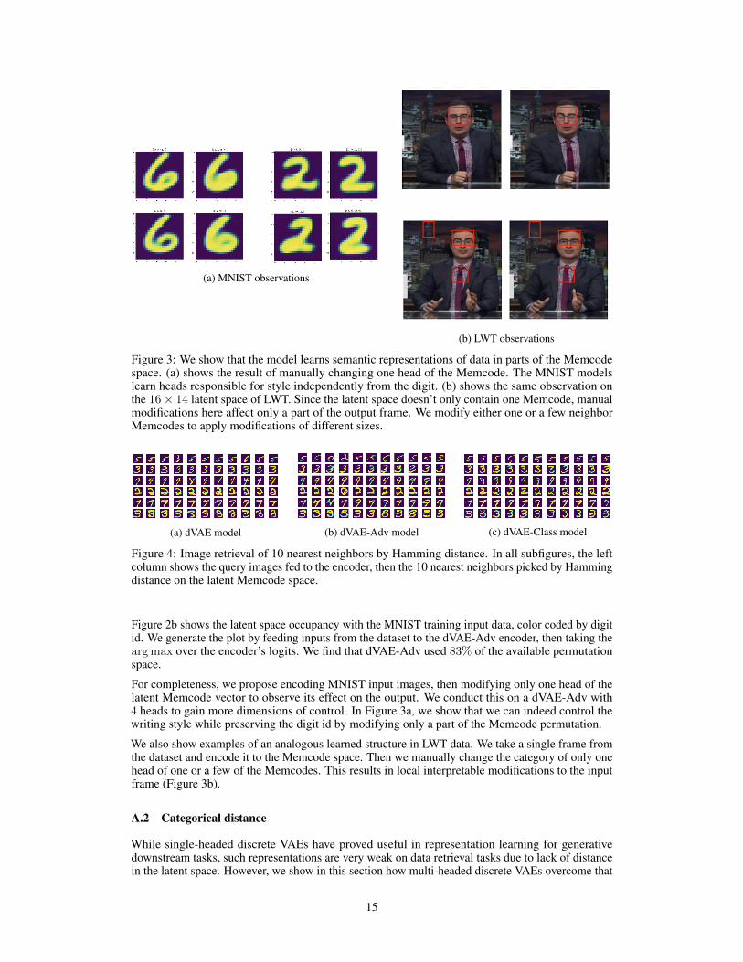
(a) MNIST observations
(b) LWT observations
Figure 3: We show that the model learns semantic representations of data in parts of the Memcodespace. (a) shows the result of manually changing one head of the Memcode. The MNIST modelslearn heads responsible for style independently from the digit. (b) shows the same observation onthe 16× 14 latent space of LWT. Since the latent space doesn’t only contain one Memcode, manualmodifications here affect only a part of the output frame. We modify either one or a few neighborMemcodes to apply modifications of different sizes.
(a) dVAE model (b) dVAE-Adv model (c) dVAE-Class model
Figure 4: Image retrieval of 10 nearest neighbors by Hamming distance. In all subfigures, the leftcolumn shows the query images fed to the encoder, then the 10 nearest neighbors picked by Hammingdistance on the latent Memcode space.
Figure 2b shows the latent space occupancy with the MNIST training input data, color coded by digitid. We generate the plot by feeding inputs from the dataset to the dVAE-Adv encoder, then taking theargmax over the encoder’s logits. We find that dVAE-Adv used 83% of the available permutationspace.
For completeness, we propose encoding MNIST input images, then modifying only one head of thelatent Memcode vector to observe its effect on the output. We conduct this on a dVAE-Adv with4 heads to gain more dimensions of control. In Figure 3a, we show that we can indeed control thewriting style while preserving the digit id by modifying only a part of the Memcode permutation.
We also show examples of an analogous learned structure in LWT data. We take a single frame fromthe dataset and encode it to the Memcode space. Then we manually change the category of only onehead of one or a few of the Memcodes. This results in local interpretable modifications to the inputframe (Figure 3b).
A.2 Categorical distance
While single-headed discrete VAEs have proved useful in representation learning for generativedownstream tasks, such representations are very weak on data retrieval tasks due to lack of distancein the latent space. However, we show in this section how multi-headed discrete VAEs overcome that
15

problem by implicitly learning a distance that is highly correlated to the loss function used to trainthe VAE.
We define the distance computed between two Memcodes z1 and z2 as the Hamming distance:
Lham =1
h
h−1∑i=0
(z1i 6= z2i) (10)
Two Memcodes are considered closer if they have more heads in common. This does not assume thatall data samples with similar features share the same heads, but that samples which do share headsshould have definable characteristics in common in the pixel space. The same distance was also usedin content-based image retrieval with binary autoencoders [31].
Since the Hamming distance’s resolution depends on the number of heads, we train dVAE-Adv onMNIST with a latent space of 1 × 1, a codebook of size N = 2 and 11 heads (total number ofpermutations 211).
To build an intuition around what the Hamming distance represents in practice, we propose feeding aset of inputs to dVAE-Adv’s encoder and doing argmax sampling on its probabilities for every image.We then compute Lham against every other sample in the data and we plot the nearest neighbors byHamming distance in ascending order.
Figure 4a shows the results of nearest neighbors selection on our models trained with the ELBO lossfrom (4). We notice that the model clusters samples together based on image similarity on the pixelspace. i.e, digits that occupy the same regions in the pixel domain tend to be clustered together in theMemcode domain. This may be due to images having similar degrees of rotation, similar boldness oreven similar digits. To quantify the extent to which this metric groups digits together, we compute thezero-shot Hamming distance nearest neighbor classification and get a 75.3% accuracy on the test set.
We then train the same model using the generator loss from (8) where Lrecon is computed acrossall but the output layer of the critic. We show the results in Figure 4b. We observe that this modelclusters the images less by their similarity on the pixel domain, and more by their likelihood to sharefeatures. i.e, the generator clusters images by their similarity on the critic’s feature maps. Since digitsshare features between each other, we find that this model’s clustering still does not correlate with thedigits ids perfectly, which is confirmed by a 76.9% accuracy by zero-shot Hamming distance nearestneighbor classification.
Finally, we propose modifying the critic from dVAE-Adv to also play the role of a digit classifier. Wecall this full model dVAE-Class. To do so, we add a second output layer to the critic and add a digitclassification cross entropy to (9). We note that both critic output layers use the same activations fromthe penultimate layer as input. We also only optimize Lrecon on the penultimate layer’s activations.We assume that a digit classifier discards sample specific information and only keeps digit id relevantinformation in the penultimate layer. We show the results of this model in Figure 4c.
In contrast to previous experiments, dVAE-Class clearly clusters the images by digit id and much lessby other sample specific features. This is also reflected in a 94.7% accuracy by zero-shot Hammingdistance nearest neighbor classification, compared to 97.3% accuracy by the critic classifier. Weachieve very similar results by training the generator on the penultimate layer’s activations of apre-trained MNIST classifier, without use of a critic.
These observations encourage us to use a multi-headed categorical distribution over the latent spaceon generation tasks, since wrongly predicting one of the heads should still generate an output thatis close to the target, where the distance depends on the dVAE loss function. We believe that thisdistance property could also be useful in other clustering tasks where one can design the loss functionto create specific data clusters.
16

B Model architectures
B.1 dVAE-Adv
A variational autoencoder trained to compress and reconstruct videos.
B.1.1 Encoder
The dVAE-Adv encoder starts by spatially downsampling the input video on each frame independentlyusing 2D residual blocks [17] followed by a strided convolution [4]. If the number of filters changesin the residual block, we use a shortcut 1× 1 conv in the residual branch. After extracting the spatialfeature maps for each frame, we compute the temporal feature maps across frames using a temporalblock consisting of a stack of 3D convolutions. We found the temporal block necessary to removeflicker and prevent jitteriness. A large temporal receptive field was not necessary in our experiments.Note that we do not compress the video clip along the time dimension.
B.1.2 Hard attention discretization layer
The encoder outputs (temporal feature maps) are used as the query sequence Q for the multi-headhard attention block. The keys K and values V sequences are separate linear projections of anembedding space e ∈ RN×D where D is the dimensionality of the embedding codebook. Themulti-head hard attention block looks up the embedding table h times (the number of attention heads)for each Memcode. The attention is computed independently between each element of the queriessequence Q, and is computed against all rows of the embedding space e.
B.1.3 Decoder
The output of the multi-head hard attention is used as the decoder input. The decoder is a mirroredversion of the encoder. We first compute the temporal feature maps using a similar architecture to theencoder’s temporal block. To output in the original video resolution, we use a 2D nearest neighborupsampling layer [40] followed by residual blocks that operate on each frame independently. Thereconstructed spatial feature maps are then passed to a tanh output layer for the final pixel values.
B.1.4 Critics
For the critics, we design each model as a Markovian window-based adversary (analogous to imagepatches [22, 33]) consisting of a sequence of strided convolutional layers. We ensure that critics havedifferent strides and receptive fields to capture multi-scale information about the videos. We alsofound it beneficial to make some of the critics operate only spatially to improve independent framequality. In all our experiments, we compute Lrecon on all but the output layers of the critics.
B.1.5 Gradient approximation
While the Memcode discretization using Gumbel-max trick as presented in (1) is equivalent to anatural sampling from the multinomial distribution (z ∼ Smax(χ)), the gradient flow during backpropagation is almost always different:
∂Smax(χ)
∂φ6= ∂Smax(χ+G)
∂φ(11)
since
∂Smax(χ)
∂φ=∂Smax(χ)
∂χ
∂χ
∂φ(12)
and
∂Smax(χ+G)
∂φ=∂Smax(χ+G)
∂(χ+G)
∂(χ+G)
∂χ︸ ︷︷ ︸=1
∂χ
∂φ=∂Smax(χ+G)
∂(χ+G)
∂χ
∂φ(13)
17

Figure 5: (Left) Softmax distribution over logits χ. (center) The same softmax distribution after theaddition of gumbel noise G. (right) Sampled z by either multinomial sampling from z ∼ Smax(χ) orargmax(Smax(χ+G)). The sample z is more likely to be sampled from Smax(χ+G) than fromSmax(χ).
where φ are the dVAE-Adv encoder parameters and the Gumbel noise G is almost always differentfrom the zero-vector 0.
We expect the model to be more stable to train when the gradient approximation is more representativeof the forward pass. From that perspective, a gradient approximation that maximizes the likelihoodof a latent z being sampled from the softmax distribution is more stable to train.
In categorical distributions, the argmax sampling guarantees maximum likelihood, which makes theGumbel-trick all the more interesting since the straight-through gradient estimation only bypasses theargmax function, instead of the whole sampling operation. This ensures that our gradients, whichdepends on the Gumbel noise, are more representative of the forward pass (Figure 5).
Empirically, we found that models trained with the Gumbel-max trick explained in (1) are more stableand converge to slightly better optimums in comparison to sampling from the softmax distribution.The former models are also less prone to gradient explosions that cause the latent space to collapse,even when trained with small batch sizes.
B.2 Prior autoregressive model
A prior autoregressive model which predicts video Memcodes from audio (Figure 1b).
B.2.1 Audio encoder
The audio encoder uses a sequence of convolutional layers to analyze the audio spectrogram inputsand extract useful features for the video generation task. These feature maps are then upsampledspatially using nearest neighbor upsampling and spatially connected layers. We found this upsamplingstrategy to be more stable than simply tiling the audio feature maps over the spatial dimensions.
Spatially connected layers are similar to 2D locally connected layers in space dimensions, but shareweights on the time dimension. In contrast to simple 3D convolutions, spatially connected layersbenefit from space location awareness. In practice, it is very easy to implement this layer as a patchextraction convolution with a non-trainable eye matrix kernel followed by a matrix multiplication.Such an implementation makes this layer almost as fast as a convolutions while having location awareparameters. Empirically, spatially connected layers yielded more dynamic yet more stable resultsthan a simple tile or a convolution upsample.
B.2.2 Style encoder
Similarly to Hsu et al. [20], we found it useful to include a variational latent encoder q(zl|z) thatcreates a compressed, fixed size, multivariate Gaussian latent representation of the target Memcodes.The style encoder uses a stack of convolutions to extract useful style feature maps from the targetMemcodes. To create a fixed size vector from variable length videos, we use a global average poolinglayer to aggregate the convolution feature maps. Including this variational encoder enables the modelto unsupervisedly learn a latent representation zl encoding global characteristics of the output videosthat do not correlate well with the audio input. We upsample zl using a similar approach describedabove for upsampling audio feature maps.
18
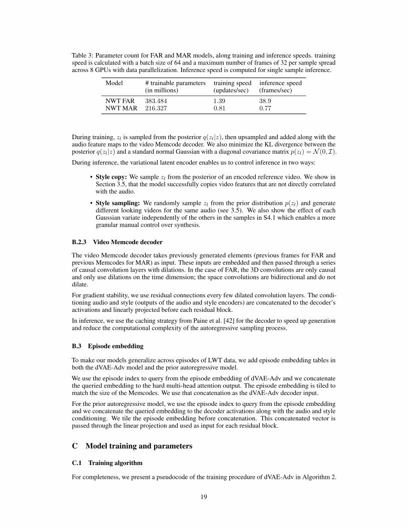
Table 3: Parameter count for FAR and MAR models, along training and inference speeds. trainingspeed is calculated with a batch size of 64 and a maximum number of frames of 32 per sample spreadacross 8 GPUs with data parallelization. Inference speed is computed for single sample inference.
Model # trainable parameters(in millions)
training speed(updates/sec)
inference speed(frames/sec)
NWT FAR 383.484 1.39 38.9NWT MAR 216.327 0.81 0.77
During training, zl is sampled from the posterior q(zl|z), then upsampled and added along with theaudio feature maps to the video Memcode decoder. We also minimize the KL divergence between theposterior q(zl|z) and a standard normal Gaussian with a diagonal covariance matrix p(zl) = N (0, I).During inference, the variational latent encoder enables us to control inference in two ways:
• Style copy: We sample zl from the posterior of an encoded reference video. We show inSection 3.5, that the model successfully copies video features that are not directly correlatedwith the audio.
• Style sampling: We randomly sample zl from the prior distribution p(zl) and generatedifferent looking videos for the same audio (see 3.5). We also show the effect of eachGaussian variate independently of the others in the samples in S4.1 which enables a moregranular manual control over synthesis.
B.2.3 Video Memcode decoder
The video Memcode decoder takes previously generated elements (previous frames for FAR andprevious Memcodes for MAR) as input. These inputs are embedded and then passed through a seriesof causal convolution layers with dilations. In the case of FAR, the 3D convolutions are only causaland only use dilations on the time dimension; the space convolutions are bidirectional and do notdilate.
For gradient stability, we use residual connections every few dilated convolution layers. The condi-tioning audio and style (outputs of the audio and style encoders) are concatenated to the decoder’sactivations and linearly projected before each residual block.
In inference, we use the caching strategy from Paine et al. [42] for the decoder to speed up generationand reduce the computational complexity of the autoregressive sampling process.
B.3 Episode embedding
To make our models generalize across episodes of LWT data, we add episode embedding tables inboth the dVAE-Adv model and the prior autoregressive model.
We use the episode index to query from the episode embedding of dVAE-Adv and we concatenatethe queried embedding to the hard multi-head attention output. The episode embedding is tiled tomatch the size of the Memcodes. We use that concatenation as the dVAE-Adv decoder input.
For the prior autoregressive model, we use the episode index to query from the episode embeddingand we concatenate the queried embedding to the decoder activations along with the audio and styleconditioning. We tile the episode embedding before concatenation. This concatenated vector ispassed through the linear projection and used as input for each residual block.
C Model training and parameters
C.1 Training algorithm
For completeness, we present a pseudocode of the training procedure of dVAE-Adv in Algorithm 2.
19
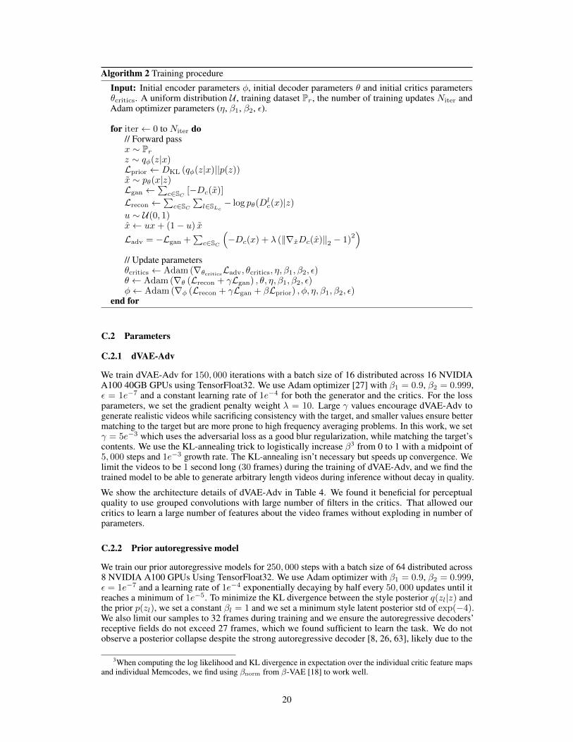
Algorithm 2 Training procedure
Input: Initial encoder parameters φ, initial decoder parameters θ and initial critics parametersθcritics. A uniform distribution U , training dataset Pr, the number of training updates Niter andAdam optimizer parameters (η, β1, β2, ε).
for iter← 0 to Niter do// Forward passx ∼ Prz ∼ qφ(z|x)Lprior ← DKL (qφ(z|x)||p(z))x̃ ∼ pθ(x|z)Lgan ←
∑c∈SC [−Dc(x̃)]
Lrecon ←∑c∈SC
∑l∈SLc
− log pθ(Dlc(x)|z)
u ∼ U(0, 1)x̂← ux+ (1− u) x̃Ladv = −Lgan +
∑c∈SC
(−Dc(x) + λ (‖∇x̂Dc(x̂)‖2 − 1)
2)
// Update parametersθcritics ← Adam (∇θcriticsLadv, θcritics, η, β1, β2, ε)θ ← Adam (∇θ (Lrecon + γLgan) , θ, η, β1, β2, ε)φ← Adam (∇φ (Lrecon + γLgan + βLprior) , φ, η, β1, β2, ε)
end for
C.2 Parameters
C.2.1 dVAE-Adv
We train dVAE-Adv for 150, 000 iterations with a batch size of 16 distributed across 16 NVIDIAA100 40GB GPUs using TensorFloat32. We use Adam optimizer [27] with β1 = 0.9, β2 = 0.999,ε = 1e−7 and a constant learning rate of 1e−4 for both the generator and the critics. For the lossparameters, we set the gradient penalty weight λ = 10. Large γ values encourage dVAE-Adv togenerate realistic videos while sacrificing consistency with the target, and smaller values ensure bettermatching to the target but are more prone to high frequency averaging problems. In this work, we setγ = 5e−3 which uses the adversarial loss as a good blur regularization, while matching the target’scontents. We use the KL-annealing trick to logistically increase β3 from 0 to 1 with a midpoint of5, 000 steps and 1e−3 growth rate. The KL-annealing isn’t necessary but speeds up convergence. Welimit the videos to be 1 second long (30 frames) during the training of dVAE-Adv, and we find thetrained model to be able to generate arbitrary length videos during inference without decay in quality.
We show the architecture details of dVAE-Adv in Table 4. We found it beneficial for perceptualquality to use grouped convolutions with large number of filters in the critics. That allowed ourcritics to learn a large number of features about the video frames without exploding in number ofparameters.
C.2.2 Prior autoregressive model
We train our prior autoregressive models for 250, 000 steps with a batch size of 64 distributed across8 NVIDIA A100 GPUs Using TensorFloat32. We use Adam optimizer with β1 = 0.9, β2 = 0.999,ε = 1e−7 and a learning rate of 1e−4 exponentially decaying by half every 50, 000 updates until itreaches a minimum of 1e−5. To minimize the KL divergence between the style posterior q(zl|z) andthe prior p(zl), we set a constant βl = 1 and we set a minimum style latent posterior std of exp(−4).We also limit our samples to 32 frames during training and we ensure the autoregressive decoders’receptive fields do not exceed 27 frames, which we found sufficient to learn the task. We do notobserve a posterior collapse despite the strong autoregressive decoder [8, 26, 63], likely due to the
3When computing the log likelihood and KL divergence in expectation over the individual critic feature mapsand individual Memcodes, we find using βnorm from β-VAE [18] to work well.
20
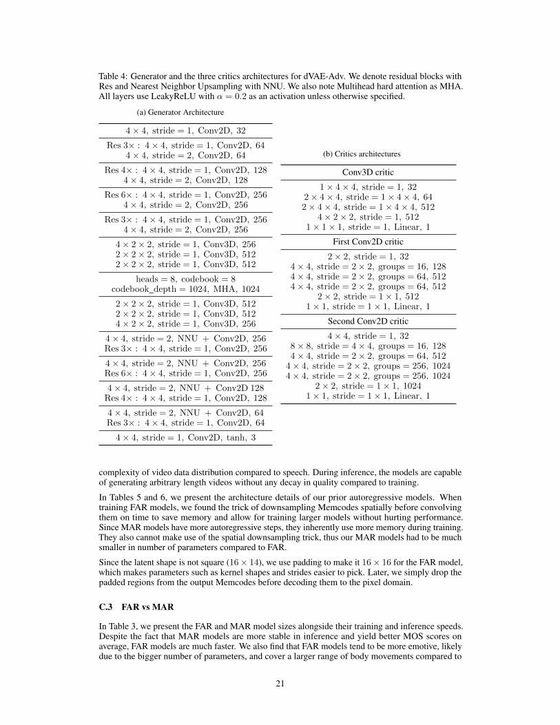
Table 4: Generator and the three critics architectures for dVAE-Adv. We denote residual blocks withRes and Nearest Neighbor Upsampling with NNU. We also note Multihead hard attention as MHA.All layers use LeakyReLU with α = 0.2 as an activation unless otherwise specified.
(a) Generator Architecture
4× 4, stride = 1, Conv2D, 32
Res 3× : 4× 4, stride = 1, Conv2D, 644× 4, stride = 2, Conv2D, 64
Res 4× : 4× 4, stride = 1, Conv2D, 1284× 4, stride = 2, Conv2D, 128
Res 6× : 4× 4, stride = 1, Conv2D, 2564× 4, stride = 2, Conv2D, 256
Res 3× : 4× 4, stride = 1, Conv2D, 2564× 4, stride = 2, Conv2D, 256
4× 2× 2, stride = 1, Conv3D, 2562× 2× 2, stride = 1, Conv3D, 5122× 2× 2, stride = 1, Conv3D, 512
heads = 8, codebook = 8codebook_depth = 1024, MHA, 1024
2× 2× 2, stride = 1, Conv3D, 5122× 2× 2, stride = 1, Conv3D, 5124× 2× 2, stride = 1, Conv3D, 256
4× 4, stride = 2, NNU + Conv2D, 256Res 3× : 4× 4, stride = 1, Conv2D, 256
4× 4, stride = 2, NNU + Conv2D, 256Res 6× : 4× 4, stride = 1, Conv2D, 256
4× 4, stride = 2, NNU + Conv2D 128Res 4× : 4× 4, stride = 1, Conv2D, 128
4× 4, stride = 2, NNU + Conv2D, 64Res 3× : 4× 4, stride = 1, Conv2D, 64
4× 4, stride = 1, Conv2D, tanh, 3
(b) Critics architectures
Conv3D critic
1× 4× 4, stride = 1, 322× 4× 4, stride = 1× 4× 4, 642× 4× 4, stride = 1× 4× 4, 512
4× 2× 2, stride = 1, 5121× 1× 1, stride = 1, Linear, 1
First Conv2D critic
2× 2, stride = 1, 324× 4, stride = 2× 2, groups = 16, 1284× 4, stride = 2× 2, groups = 64, 5124× 4, stride = 2× 2, groups = 64, 512
2× 2, stride = 1× 1, 5121× 1, stride = 1× 1, Linear, 1
Second Conv2D critic
4× 4, stride = 1, 328× 8, stride = 4× 4, groups = 16, 1284× 4, stride = 2× 2, groups = 64, 5124× 4, stride = 2× 2, groups = 256, 10244× 4, stride = 2× 2, groups = 256, 1024
2× 2, stride = 1× 1, 10241× 1, stride = 1× 1, Linear, 1
complexity of video data distribution compared to speech. During inference, the models are capableof generating arbitrary length videos without any decay in quality compared to training.
In Tables 5 and 6, we present the architecture details of our prior autoregressive models. Whentraining FAR models, we found the trick of downsampling Memcodes spatially before convolvingthem on time to save memory and allow for training larger models without hurting performance.Since MAR models have more autoregressive steps, they inherently use more memory during training.They also cannot make use of the spatial downsampling trick, thus our MAR models had to be muchsmaller in number of parameters compared to FAR.
Since the latent shape is not square (16× 14), we use padding to make it 16× 16 for the FAR model,which makes parameters such as kernel shapes and strides easier to pick. Later, we simply drop thepadded regions from the output Memcodes before decoding them to the pixel domain.
C.3 FAR vs MAR
In Table 3, we present the FAR and MAR model sizes alongside their training and inference speeds.Despite the fact that MAR models are more stable in inference and yield better MOS scores onaverage, FAR models are much faster. We also find that FAR models tend to be more emotive, likelydue to the bigger number of parameters, and cover a larger range of body movements compared to
21
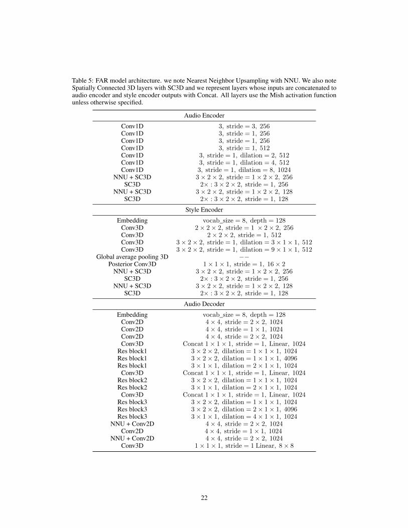
Table 5: FAR model architecture. we note Nearest Neighbor Upsampling with NNU. We also noteSpatially Connected 3D layers with SC3D and we represent layers whose inputs are concatenated toaudio encoder and style encoder outputs with Concat. All layers use the Mish activation functionunless otherwise specified.
Audio Encoder
Conv1D 3, stride = 3, 256Conv1D 3, stride = 1, 256Conv1D 3, stride = 1, 256Conv1D 3, stride = 1, 512Conv1D 3, stride = 1, dilation = 2, 512Conv1D 3, stride = 1, dilation = 4, 512Conv1D 3, stride = 1, dilation = 8, 1024
NNU + SC3D 3× 2× 2, stride = 1× 2× 2, 256SC3D 2× : 3× 2× 2, stride = 1, 256
NNU + SC3D 3× 2× 2, stride = 1× 2× 2, 128SC3D 2× : 3× 2× 2, stride = 1, 128
Style Encoder
Embedding vocab_size = 8, depth = 128Conv3D 2× 2× 2, stride = 1 × 2× 2, 256Conv3D 2× 2× 2, stride = 1, 512Conv3D 3× 2× 2, stride = 1, dilation = 3× 1× 1, 512Conv3D 3× 2× 2, stride = 1, dilation = 9× 1× 1, 512
Global average pooling 3D −−Posterior Conv3D 1× 1× 1, stride = 1, 16× 2
NNU + SC3D 3× 2× 2, stride = 1× 2× 2, 256SC3D 2× : 3× 2× 2, stride = 1, 256
NNU + SC3D 3× 2× 2, stride = 1× 2× 2, 128SC3D 2× : 3× 2× 2, stride = 1, 128
Audio Decoder
Embedding vocab_size = 8, depth = 128Conv2D 4× 4, stride = 2× 2, 1024Conv2D 4× 4, stride = 1× 1, 1024Conv2D 4× 4, stride = 2× 2, 1024Conv3D Concat 1× 1× 1, stride = 1, Linear, 1024
Res block1 3× 2× 2, dilation = 1× 1× 1, 1024Res block1 3× 2× 2, dilation = 1× 1× 1, 4096Res block1 3× 1× 1, dilation = 2× 1× 1, 1024
Conv3D Concat 1× 1× 1, stride = 1, Linear, 1024Res block2 3× 2× 2, dilation = 1× 1× 1, 1024Res block2 3× 1× 1, dilation = 2× 1× 1, 1024
Conv3D Concat 1× 1× 1, stride = 1, Linear, 1024Res block3 3× 2× 2, dilation = 1× 1× 1, 1024Res block3 3× 2× 2, dilation = 2× 1× 1, 4096Res block3 3× 1× 1, dilation = 4× 1× 1, 1024
NNU + Conv2D 4× 4, stride = 2× 2, 1024Conv2D 4× 4, stride = 1× 1, 1024
NNU + Conv2D 4× 4, stride = 2× 2, 1024Conv3D 1× 1× 1, stride = 1 Linear, 8× 8
22
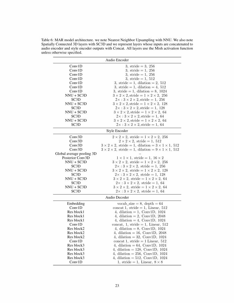
Table 6: MAR model architecture. we note Nearest Neighbor Upsampling with NNU. We also noteSpatially Connected 3D layers with SC3D and we represent layers whose inputs are concatenated toaudio encoder and style encoder outputs with Concat. All layers use the Mish activation functionunless otherwise specified.
Audio Encoder
Conv1D 3, stride = 3, 256Conv1D 3, stride = 1, 256Conv1D 3, stride = 1, 256Conv1D 3, stride = 1, 512Conv1D 3, stride = 1, dilation = 2, 512Conv1D 3, stride = 1, dilation = 4, 512Conv1D 3, stride = 1, dilation = 8, 1024
NNU + SC3D 3× 2× 2, stride = 1× 2× 2, 256SC3D 2× : 3× 2× 2, stride = 1, 256
NNU + SC3D 3× 2× 2, stride = 1× 2× 2, 128SC3D 2× : 3× 2× 2, stride = 1, 128
NNU + SC3D 3× 2× 2, stride = 1× 2× 2, 64SC3D 2× : 3× 2× 2, stride = 1, 64
NNU + SC3D 3× 2× 2, stride = 1× 2× 2, 64SC3D 2× : 3× 2× 2, stride = 1, 64
Style Encoder
Conv3D 2× 2× 2, stride = 1× 2× 2, 256Conv3D 2× 2× 2, stride = 1, 512Conv3D 3× 2× 2, stride = 1, dilation = 3× 1× 1, 512Conv3D 3× 2× 2, stride = 1, dilation = 9× 1× 1, 512
Global average pooling 3D –Posterior Conv3D 1× 1× 1, stride = 1, 16× 2
NNU + SC3D 3× 2× 2, stride = 1× 2× 2, 256SC3D 2× : 3× 2× 2, stride = 1, 256
NNU + SC3D 3× 2× 2, stride = 1× 2× 2, 128SC3D 2× : 3× 2× 2, stride = 1, 128
NNU + SC3D 3× 2× 2, stride = 1× 2× 2, 64SC3D 2× : 3× 2× 2, stride = 1, 64
NNU + SC3D 3× 2× 2, stride = 1× 2× 2, 64SC3D 2× : 3× 2× 2, stride = 1, 64
Audio Decoder
Embedding vocab_size = 8, depth = 64Conv1D concat 1, stride = 1, Linear, 512
Res block1 4, dilation = 1, Conv1D, 1024Res block1 4, dilation = 2, Conv1D, 2048Res block1 4, dilation = 4, Conv1D, 1024
Conv1D concat, 1, stride = 1, Linear, 512Res block2 4, dilation = 8, Conv1D, 1024Res block2 4, dilation = 16, Conv1D, 2048Res block2 4, dilation = 32, Conv1D, 1024
Conv1D concat 1, stride = 1 Linear, 512Res block3 4, dilation = 64, Conv1D, 1024Res block3 4, dilation = 128, Conv1D, 1024Res block3 4, dilation = 256, Conv1D, 1024Res block3 4, dilation = 512, Conv1D, 1024
Conv1D 1, stride = 1, Linear, 8× 8
23

MAR. We find it useful to have both models for different use cases; where FAR is usable in real timeinference, MAR would be a better choice on large scale slow video inference.
D Data preparation
We prepared our dataset by the following procedure:
1. download videos using youtube-dl given a list of 219 video URLs, all sourced fromthe official Last Week Tonight channel on YouTube: https://www.youtube.com/user/LastWeekTonight.
2. split episodes using H.264 codec key frames as boundaries, which divides videos intosegments of a maximum of 8.37 seconds using ffmpeg:
$ ffmpeg −y − i $INPUT_FILEPATH \− acodec copy − f segment − segmen t_ t ime 4 \−vcodec copy − r e s e t _ t i m e s t a m p s 1 −map 0 \$OUTPUT_FILEPATH
3. crop videos from 507 to 1130 left to right, and 0 to 712 bottom to top.4. for every clip greater than 2 seconds, trim 0.25 seconds from the beginning and end, resulting
in a maximum clip duration of 7.87 seconds5. manually review to remove clips where any of the following occur
• subject is not in frame• subject is holding objects• there are person(s) other than subject visible• there are intruding overlays inserted in post production• there is a title screen transition• subject is not sitting at desk, e.g. standing or conducting an interview
6. To protect our models from trying to learn the seemingly random side overlays in the videos,we apply an algorithmic heuristic to mask them using the following OpenCV [9] functions.The following is applied to each frame in every video of the dataset:(a) convert frame to grayscale
gray_image = cv2.cvtColor(color_image, cv2.COLOR_BGR2GRAY)(b) binarize the frame
binarized_image = cv2.threshold(gray_image, 185, 255, 0)[1](c) find contours
contours = cv2.findContours(binarized_image, cv2.RETR_EXTERNAL,cv2.CHAIN_APPROX_SIMPLE)[0]
(d) for each contour, find the bounding rectanglex, y, w, h = cv2.boundingRect(contour)
(e) for each bounding rectangle, if the area is greater than 4000 pixels, smaller than 100000pixels, has a height greater than 80 pixels, and the top left corner of the bounding boxeither within 20 pixels from the left hand side of the frame, or starts more than 550pixels from the top of the frame, then this bounding box is used to overlay the originalframe with a white rectangle.
7. using moviepy, scale clips to 256 × 224 and interpolate to 30 frames per second (FPS),preserving duration (downloaded data contains a mix of frame rates including 30000
1001 and 30FPS).
8. extract audio from video clips, interpolating to a sample rate of 24000, convert to mono andgenerate Mel spectrograms using the parameters in Table 7.
9. Scale video pixels to a range of [−1, 1] with min-max scaling: x = x127.5 − 1
10. split into train, validation, and test sets stratified by episodes with ratios of approximately90%, 5%, and 5% respectively.
24
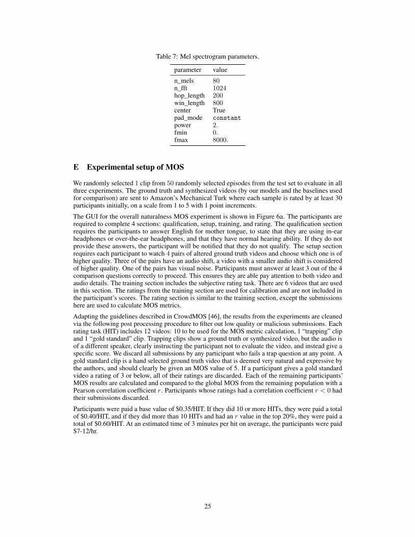
Table 7: Mel spectrogram parameters.
parameter value
n_mels 80n_fft 1024hop_length 200win_length 800center Truepad_mode constantpower 2.fmin 0.fmax 8000.
E Experimental setup of MOS
We randomly selected 1 clip from 50 randomly selected episodes from the test set to evaluate in allthree experiments. The ground truth and synthesized videos (by our models and the baselines usedfor comparison) are sent to Amazon’s Mechanical Turk where each sample is rated by at least 30participants initially, on a scale from 1 to 5 with 1 point increments.
The GUI for the overall naturalness MOS experiment is shown in Figure 6a. The participants arerequired to complete 4 sections: qualification, setup, training, and rating. The qualification sectionrequires the participants to answer English for mother tongue, to state that they are using in-earheadphones or over-the-ear headphones, and that they have normal hearing ability. If they do notprovide these answers, the participant will be notified that they do not qualify. The setup sectionrequires each participant to watch 4 pairs of altered ground truth videos and choose which one is ofhigher quality. Three of the pairs have an audio shift, a video with a smaller audio shift is consideredof higher quality. One of the pairs has visual noise. Participants must answer at least 3 out of the 4comparison questions correctly to proceed. This ensures they are able pay attention to both video andaudio details. The training section includes the subjective rating task. There are 6 videos that are usedin this section. The ratings from the training section are used for calibration and are not included inthe participant’s scores. The rating section is similar to the training section, except the submissionshere are used to calculate MOS metrics.
Adapting the guidelines described in CrowdMOS [46], the results from the experiments are cleanedvia the following post processing procedure to filter out low quality or malicious submissions. Eachrating task (HIT) includes 12 videos: 10 to be used for the MOS metric calculation, 1 “trapping” clipand 1 “gold standard” clip. Trapping clips show a ground truth or synthesized video, but the audio isof a different speaker, clearly instructing the participant not to evaluate the video, and instead give aspecific score. We discard all submissions by any participant who fails a trap question at any point. Agold standard clip is a hand selected ground truth video that is deemed very natural and expressive bythe authors, and should clearly be given an MOS value of 5. If a participant gives a gold standardvideo a rating of 3 or below, all of their ratings are discarded. Each of the remaining participants’MOS results are calculated and compared to the global MOS from the remaining population with aPearson correlation coefficient r. Participants whose ratings had a correlation coefficient r < 0 hadtheir submissions discarded.
Participants were paid a base value of $0.35/HIT. If they did 10 or more HITs, they were paid a totalof $0.40/HIT, and if they did more than 10 HITs and had an r value in the top 20%, they were paid atotal of $0.60/HIT. At an estimated time of 3 minutes per hit on average, the participants were paid$7-12/hr.
25

(a) Instructions
26

(b) Qualification
27
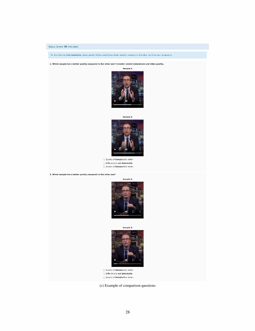
(c) Example of comparison questions
28

(d) Periodic training
29

(e) Ratings page example
Figure 6: Mechanical Turk GUI screenshots
30