numerical resolution of the boundary integral equations for elastic scattering by a plane crack
TRANSCRIPT
INTERNATIONAL JOURNAL FOR NUMERICAL METHODS IN ENGINEERING, VOL. 38, 2347-2371 (1995)
NUMERICAL RESOLUTION OF THE BOUNDARY INTEGRAL EQUATIONS FOR ELASTIC
SCATTERING BY A PLANE CRACK
CARLOS ALVES
CMAP, Ecole Polytechnique, 91 128 Palaiseau, France and Instituto Superior Ticnico, Av. Rovisco Pais, 1096 Lisboa, Portugal
TUONGHADUONG
CMAP, Ecole Polytechnique, 91 128 Palaiseau; France and Universite de Technologie de Compit?gne, 60206 Compiegne, France
SUMMARY The problem of wave scattering by a plane crack is solved, either in the case of acoustic waves or in the case of elastic waves incidence using the boundary integral equation method. A collocation method is often used to solve that equation, but here we will use a variational method, first writing the problem of Fourier variables, and then writing the associated integrals in the sesquilinear form with weak singularity kernels. This representation is used in the numerical approach, made with a finite element method in the surface of the crack. Numerical tests were made with circular and elliptical cracks, but this method can be extended to other shapes, with the same convergence profiles. Extensive results are given concerning the crack opening displacement, the scattering cross-section, the back-scattered amplitude and far-field patterns.
KEY WORDS: acoustic; elastic; scattering; crack; integral equations
0. INTRODUCTION
Three-dimensional scattering of acoustic and elastic waves by cracks is an effective problem in non-destructive testing of materials. This problem has been treated numerically by several authors in the second half of this century, namely the early works of Bouwkamp' and Jones' for the acoustic case, and later the work of Ma1 (e.g. Reference 3) for the elastic case. Different approaches have been made, for instances, the use of Fourier expansions has permitted to obtain some exact analytical solutions for some particular cases, and in more recent works the main tool is the associated boundary integral equation (BIE) for the crack opening displacement (COD). However, this BIE has two clear difficulties, it is a first kind Fredholm integral equation, and it has a hypersingular integral. In the synthetic work of Martin and Wickham4 we can see that the previous techniques to deal with these problems transform the BIE into a more treatable second kind integral equation or to a Neumann's series problem. Regularization techniques to calculate the hypersingular integral have also been more recently investigated (e.g. References 5 and 6). Another way to deal with the singularities appearing in the BIE is to use a variational formulation for the integral equation. The method indicated by Nedelec, permits to transform hypersingular integrals to weak singular ones (cf. Reference 7-9). In the case of a plane crack, Ha Duong' used
CCC 0029-59811951142347-25 0 1995 by John Wiley & Sons, Ltd.
Received 23 February 1994 Revised 13 June 1994
2348 C. ALVES AND T. H. DUONG
the partial Fourier transform to prove the coerciveness of the sesquilinear form in a suitable Sobolev space, which assures a good behaviour of the associated numerical problem, using boundary finite element methods. This approach has a higher cost in the calculation of double integrals, which is balanced by a high stability and by an inferior need of thinner triangulations, if we compare it with the other works which lead to collocation methods in solving the associated numerical problem of the BIE (cf. References 5, 11, 12, etc.). The approach taken here is tested numerically for a plane crack not necessarily of simple shape, presenting corners or cusps.
This work is divided in two distinct parts, the first one considering the acoustic problem, and the other one concerning the elastic case. A brief introduction of the mathematical problem is made in both cases, and further details are presented in Reference 10. In the elastic case, the deduction of an explicit representation of the sesquilinear form is new, and provides the numerical approach that follows. The numerical treatment of this problems in the acoustic case was presented in the master degree thesis of Alves.I3 In the elastic case, due to the presence of new kernels and the vectorial structure of the problem, some changes were improved.
We also introduce several numerical tests, validating our method by comparison with previous works and by presentation of convergence tests. The classical case of normal incident waves in the penny-shaped crack is analysed, but also the cases of oblique incidence in other different shapes, as ellipses, squares or even cardioids, in which we can see that the existence of a singular cusp does not affect our convergence profiles.
1. ACOUSTIC WAVES
1.1. Description of the problem
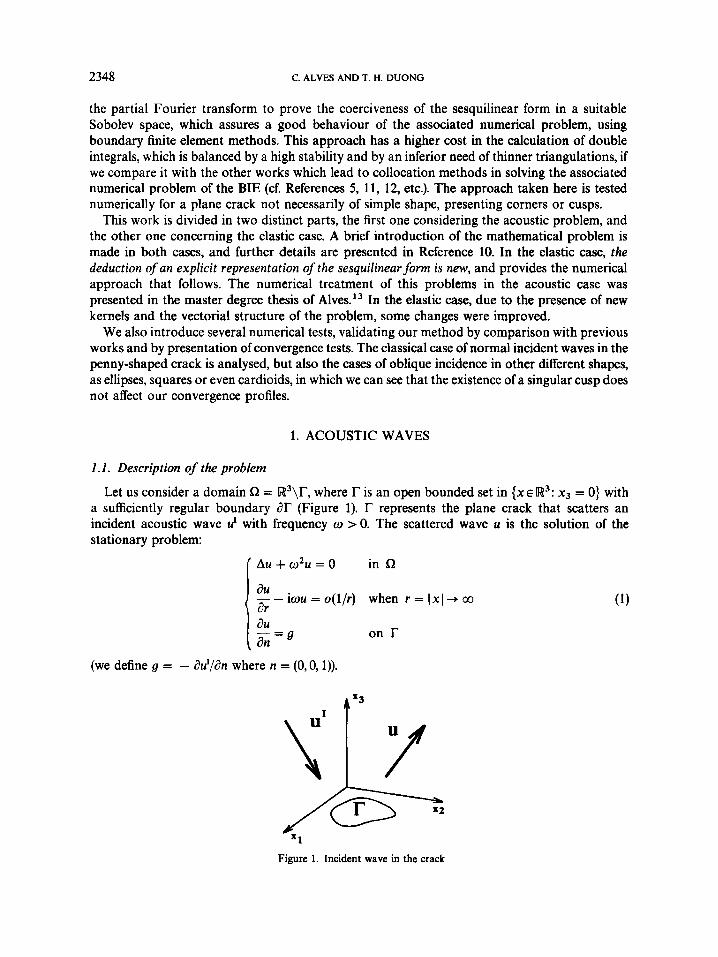
Let us consider a domain R = R3\T, where r is an open bounded set in {x E R3: x3 = 0} with a sufficiently regular boundary 8r (Figure 1). represents the plane crack that scatters an incident acoustic wave u' with frequency w > O . The scattered wave u is the solution of the stationary problem:
(we define g = ; -
A u + 0 2 u = 0 in R
iou = o(l/r) when r = 1x1 + 00
&'/an where n = (0, 0,l)).
Figure 1. Incident wave in the crack
PLANE CRACK 2349
Our solution can be written as a double-layer potential
where cp is the crack opening displacement (COD), cp( y) = u - ( y ) - u+ ( y ) = [u( y ) ] ( y E r) and G, is the Green function C,(x) = eialxl/4nlxj.
Introducing the operator
our problem is reduced to the boundary integral equation (BIE):
D q = g o n r (2)
However, this BIE involves hypersingular kernels, because a2G,/an,any = O(l / r3) ( x + 0). Considering the partial Fourier transform 94(<’) = Jp2~(x’)e-’~’’”’dx’, we can see that D has a simple expression in terms of Fourier variables, and we will be able to write a variational formulation of the problem. Introduce the functional Sobolev space H;b’(T) = {cp E H’’’(T): p - 1 / 2 q ~ L 2 ( r ) } where p denotes a positive, regular function on r, equivalent to the distance of a point in r to the boundary ar, its topology being defined by the norm
the sequilinear form b(cp, 4) = (Dcp, as
defined with duality brackets on H A f ( r ) can be written
where T(5) = - iiZ,(<) and Z,(o = + ,/m. It was shown in Reference 10 that this form of b is coercive, thus the variational problem
is well-posed for g E (HA62 (r))’, and the unique solution of the BIE (2) is the same of (3). It is worth noting that, if 4p E H#r) is continuous then cp = 0 of d r . This is the edge condition prescribed by Jones, solving the penny-shaped crack problem. Below, we will use this condition in the approximation of this Sobolev space.
1.2. Numerical approach
To deal with the numerical problem by the finite element method, an explicit representation of the sesquilinear form is needed. We can write the sesquilinear form b with weakly singular integrals (cf. Reference 9):
2350 C. ALVES AND T. H. DUONG
The approximation of this double integral with singular kernel is the main point of this paragraph. We begin by a regular triangulation f l h of rh (a polygonal set that approximates r 3 rh):
rh= u T T€.Th
where T are triangles defined by nodes aiEr (i = 1,. . . , N). We can now introduce the finite-dimensional space
Vh = { ( p h E C ( i + ) : (Phl,EP1 V T E f l h and q h = o in r \ r h } which approximates H;h2(r).
It can be easily seen that vh c H g ( r ) : Take one function P h E vh. We have ( P h E C ( r ) and (Ph piecewise H', so that fphEH'(r) c H1l2(r).
where y(x) is the closest point to x in d r , and pi(x) is the first degree polynomial equal to q,, in Ti. The integrals are singular only if the triangles Ti have points in the boundary of r, but in that case, for x sufficiently close to y(x) E X, we have
and we conclude that P - ' / ~ ( P , , E L2(r), then ( P I E ff;h2(r). V,, defined by
Bi(ai) = 6, (i, j = 1 , . . . , n) form a basis of the space V h . Our discrete variational problem leads us to the linear system [Bij] [qi] = [ I i ] , i , j = 1,. . . , n where
Let us consider n to be the number of interior nodes. Thus, the functions
n n
q ' E f d€ri
where C( T, V) = curl& T. curlBj, and
The singular kernels demand careful calculations on the integrals:
(i) I f T and U are non-adjacent triangles we can use a numerical formula for both integrations in (4) Using Gaussian point p i and weights Gi on the referential triangle f, and A = FTx + dT the affine transform of T onto f (FT represents a 2 x 2 matrix and dT a two-dimensional vector), we get
(ii) If T and U are adjacent or identical triangles, we use an analytical calculation for one integration and a numerical olte for the other. If we add and subtract 1/4n)x - yl in the Green function, we are led to one integral with non-singular kernel, which can be approximated by a numerical procedure, and to another one which can be evaluated by the
PLANE CRACK 2351
analytical calculus of the following integrals:
dy (k = 1,2). 1 xk - y k dy and I " = I r -
To evaluate this integrals, we divide the triangle Tin three subtriangles Al (I = 1,2,3) with an interior point as vertex (the Gaussian point in the numerical integration), then the value of the integral in each subtriangle is easier to calculate with polar co-ordinates in that point.
(a) Zo was already calculated in Reference 15:
e = e 3 1' ~ 1 dx = [p(log p + log(tg 8 + d m ) ) ] * , I X - Y l e = -e2
where p is the distance of the Gaussian point to the opposite edge, and 02, O3 are the angles made by the other edges with the height.
(b) To calculate Z l (or I , ) we apply the divergence theorem
IT div(v) dx = laT n, . v da, with v = [' 0 "1 E H(div, r)
(where Ei are the edges)
Tedious calculations lead us to (similar expressions for El, E z ) :
h, l x - yldo, = tIBI2a(log(M1 + Pl) - log(M0 + Po) + MIPI - MOP01
where Mi = ,/- with
T1 B 1 + B , fl= (Tl - Y, T2 - Tl) , a = IT1 - - I 2 2 - f l , 2 B = T 2 -
r o = 3 , r 1 = 7 IT2 - TlI' I T2 - Tl I (Ti = vertices of T )
1.3. Triangulation of simple cracks
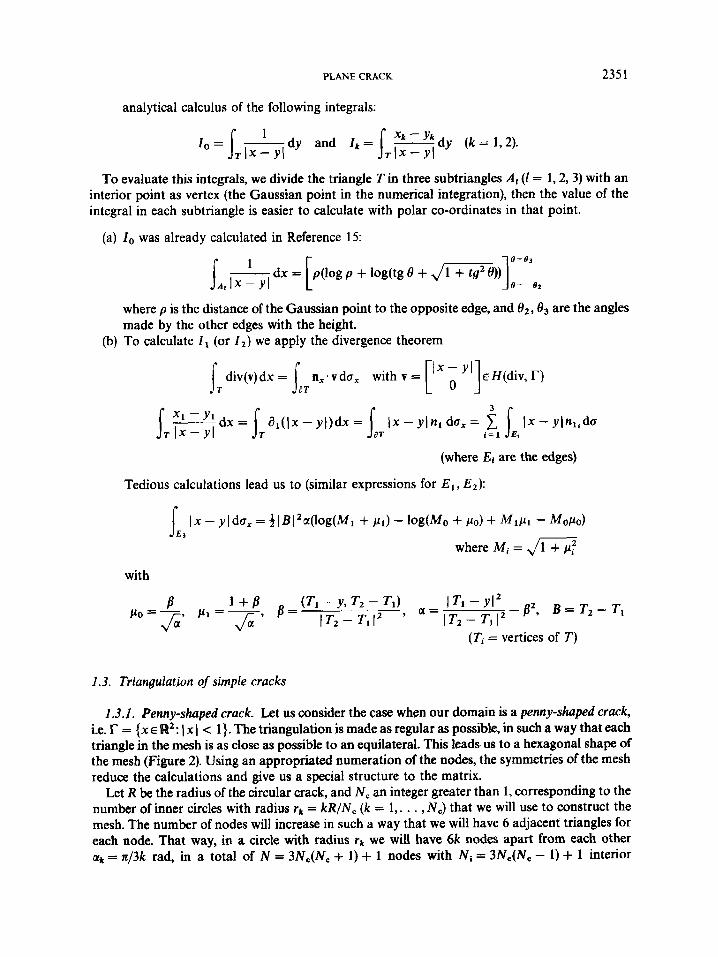
1.3.1. Penny-shaped crack. Let us consider the case when our domain is a penny-shaped crack, i.e. r = (x E 88': I x I < l}. The triangulation is made as regular as possible, in such a way that each triangle in the mesh is as close as possible to an equilateral. This leads us to a hexagonal shape of the mesh (Figure 2). Using an appropriated numeration of the nodes, the symmetries of the mesh reduce the calculations and give us a special structure ta the matrix.
Let R be the radius of the circular crack, and N , an integer greater than 1, corresponding to the number of inner circles with radius rk = k R / N , ( k = 1,. . . , N,) that we will use to construct the mesh. The number of nodes will increase in such a way that we will have 6 adjacent triangles for each node. That way, in a circle with radius rk we will have 6k nodes apart from each other ctk = n/3k rad, in a total of N = 3N,(N, + 1) + 1 nodes with Ni = 3N,(Nc - 1) + 1 interior
2352 C. ALVES AND T. H. DUONG
24 23
32 33
Figure 2. Penny-shaped crack-triangulation and numeration of the nodes with Ni = 19 ( N = 37)
nodes and N , = 6N: finite elements (Figure 2):
N, 2 3 4 5 6 7 8 Ni 7 19 37 61 91 127 169 N 19 37 61 91 127 169 217 N , 24 54 96 150 216 294 384
Let
1 cos u sin u - sinu cosu Q(4 = [
be an orthogonal rotation matrix, and 4(i) the indexes such that aq(i) = Q(k7r/3) a'. It is easy to see that we have Bij = Bq(i )q( j ) :
Consider 1 = Qx, then &x) := /3oQ'(Z) = fi(x). As Q is unitary, V,B(1) = V,p(x)Q':
curl, Pi(n). curly flj( j j ) = curl pi(x) * curl pj( y )
then
PLANE CRACK
As a consequence, our matrix will have the following Toeplitz structure:
2353
Ak are blocks M x M ( k = 1,. . . ,6), u0 is a block 1 x 1 and the ak are block M x 1. We use this fact to reduce the computation time of the matrix entries.
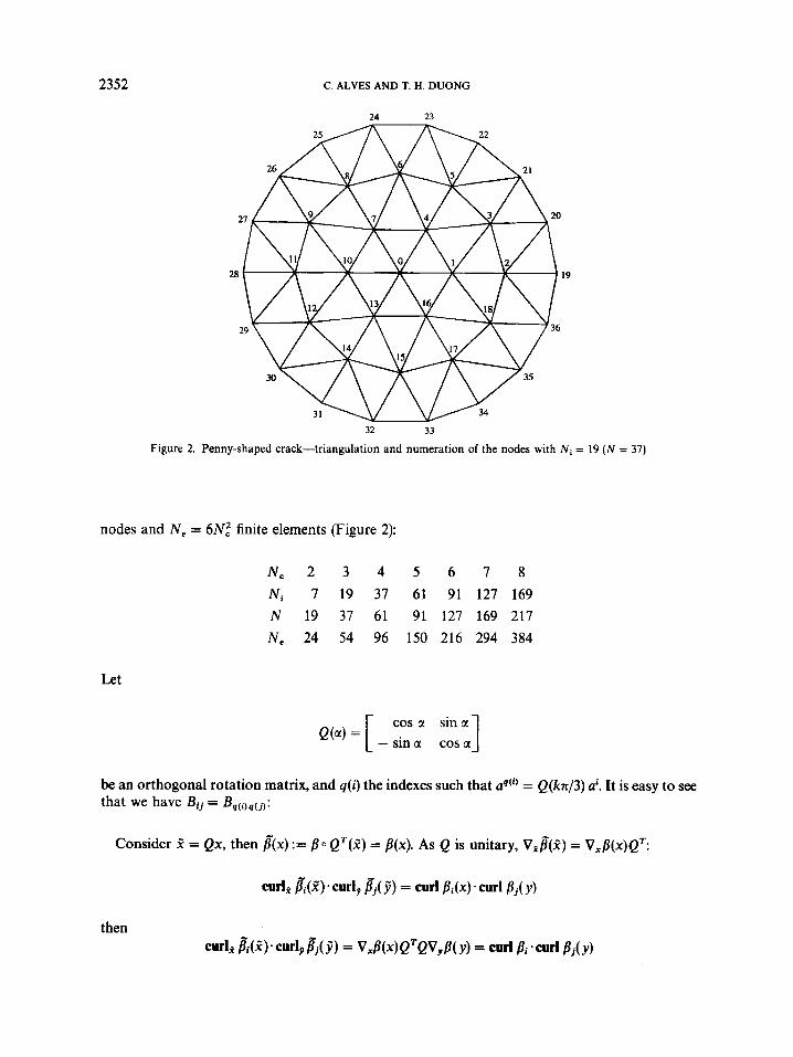
1.3.2. Elliptical and star-shaped cracks. The triangulation procedure used in the case of the penny-shaped cracks, can be extended to some other star-shaped cracks. In fact, if we consider a convenient interior point (a, b) E r, and the border X described by a parameter function y, such that
y : [ 0 , 2 n [ + [ w 2 , y(t)=(R,(t)cost +a,R2(t)s int + b )
is sufficiently regular, we are able to create inner figures
y k ( t ) = - R , ( t ) cos t + a, - R2( t ) sin t + b ) k Gc N c
in which we will put the nodes, again n/3k rad apart from each other. The mesh obtained this way, for domains other than the circle, is not the best, but the simple construction procedure allow us to use the same code in many different cracks. We show in Figure 3 some examples of this meshes.
57
Ca rdioid Square Figure 3. Triangulation procedure for other cracks, namely, a cardioid and a rectangular crack
2354 C. ALVES AND T. H. DUONG
We will be specially interested in the ellptical cracks, when R1 and R2 are constant functions, since there are results in the literature obtained for this particular kind of shapes.
1.4. Numerical tests
Let us first consider any crack scattering the incident wave:
u'(x) = eimP.x (x E R3)
where p = (sin 0,,, 0, cos 0,) is the incident wave direction. In the acoustic case, the scattering cross-section can be defined as C = II U / I $(dB1) where U is the amplitude when r -, cc (far-field), and 8B1 represents the unit sphere:
eior
U ( X ) = - r U t)( 1 + (I(:)) and U(q) =
It can be easily shown that Z = ( - l/w) Im Irg(x)@(x)dax = (440) Im o ( p ) which is the scattered power theorem, connecting the scattering cross-section and the far-field in the incidence direction.
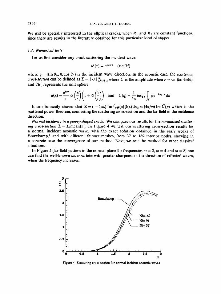
Normal incidence in a penny-shaped crack. We compare our results for the normalized scatter- ing cross-section e = X/mean(T). In Figure 4 we test our scattering cross-section results for a normal incident acoustic wave, with the exact solution obtained in the early works of Bouwkamp,' and with different thinner meshes, from 37 to 169 interior nodes, showing in a concrete case the convergence of our method. Next, we test the method for other classical situations.
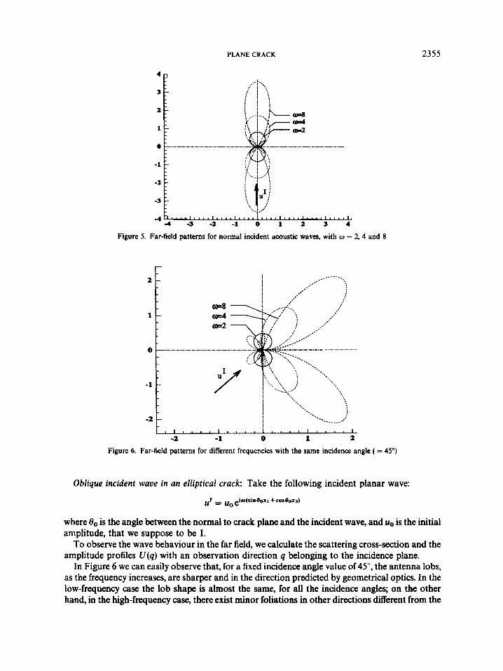
In Figure 5 (far-field pattern in the normal plane for frequencies w = 2, w = 4 and w = 8) one can find the well-known antenna lobs with greater sharpness in the direction of reflected waves, when the frequency increases.
2.5 -
2 -
1.5 -
1 -
l o , , , l * , , , l , , . , ] 0 0.5 1 1.5 2 2.5 3
W
Figure 4. Scattering cross-section for normal incident acoustic waves
PLANE CRACK 2355
Figure 5. 4 a -a -1 o 1 a 3 4
Far-field patterns for normal incident acoustic waves, with o =
r-
2, 4 and 8
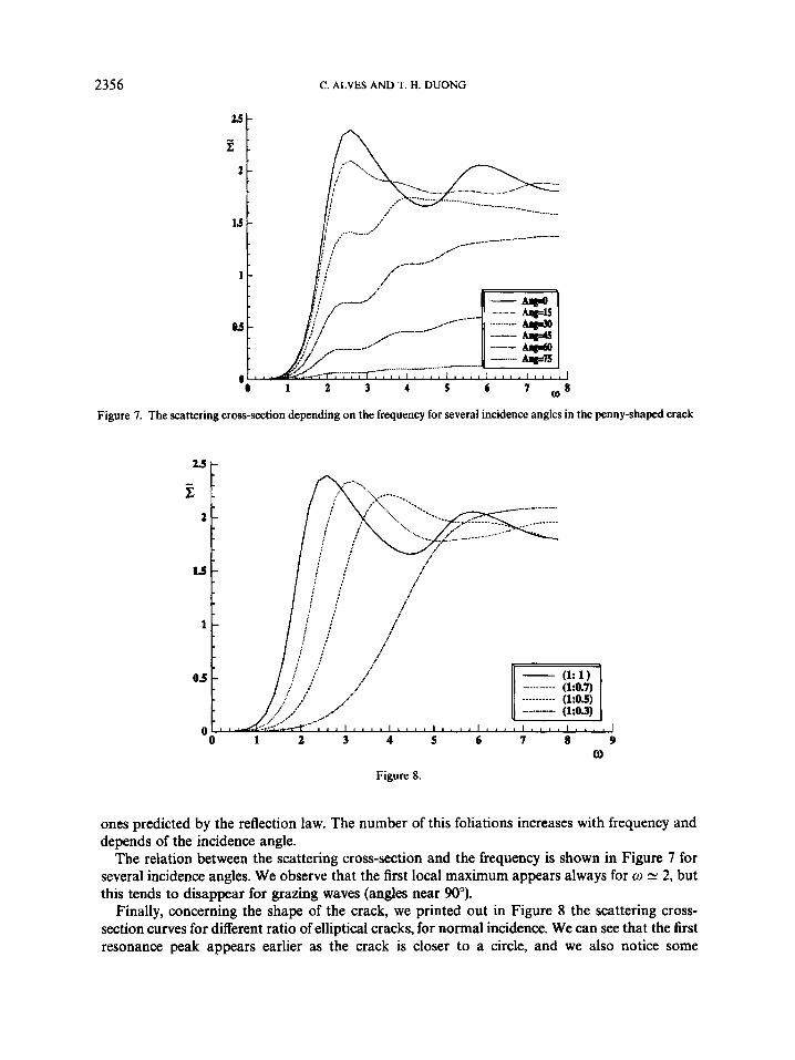
-2 -1 0 1 2
Figure 6. Far-field patterns for different frequencies with the same incidence angle ( = 45")
Oblique incident wave in an elliptical crack: Take the following incident planar wave:
uI = ug eiru(sinOoxl +COS&JXJ)
where O0 is the angle between the normal to crack plane and the incident wave, and uo is the initial amplitude, that we suppose to be 1.
To observe the wave behaviour in the far field, we calculate the scattering cross-section and the amplitude profiles U(q) with an observation direction q belonging to the incidence plane.
In Figure 6 we can easily observe that, for a fixed incidence angle value of 45", the antenna lobs, as the frequency increases, are sharper and in the direction predicted by geometrical optics. In the low-frequency case the lob shape is almost the same, for all the incidence angles; on the other hand, in the high-frequency case, there exist minor foliations in other directions different from the
2356 C. ALVES AND T. H. DUONG
E 2
_ _ . - - - - 1.5
1
0 a 1 2 3 4 6
Figure 7. The scattering cross-section depending on the frequency for several incidence angles in the penny-shaped crack
2.5 l-
0
Figure 8.
ones predicted by the reflection law. The number of this foliations increases with frequency and depends of the incidence angle.
The relation between the scattering cross-section and the frequency is shown in Figure 7 for several incidence angles. We observe that the first local maximum appears always for w N 2, but this tends to disappear for grazing waves (angles near 90O).
Finally, concerning the shape of the crack, we printed out in Figure 8 the scattering cross- section curves for different ratio of elliptical cracks, for normal incidence. We can see that the first resonance peak appears earlier as the crack is closer to a circle, and we also notice some
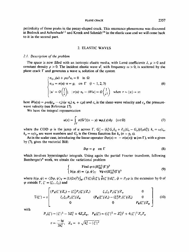
PLANE CRACK 2357
periodicity of those peaks in the penny-shaped crack. This resonance phenomena was discussed in Budreck and Achenbach“ and Krenk and SchmidtI6 in the elastic case and we will come back to it in the second part.
2. ELASTIC WAVES
2.1. Description of the problem
The space is now filled with an isotropic elastic media, with Lame coefficients 1, p > 0 and constant density p > 0. The incident elastic wave u’, with frequency o > 0, is scattered by the plane crack r and generates a wave u, solution of the system
o ~ ~ , ~ ( u ) + pw2ui = 0 in R ui3 = a(u)-n = gi on r ( i = 1,2,3)
here Wu(x) = po((c, - cs) (u 1 n,) n, + c,u) and c, is the shear-wave velocity and cp the pressure- wave velocity (see Reference 17).
We have the integral representation
where the COD cp is the jump of u across r, Gj = (k;G,ai j + di j (G, - G,))/(pk?); k, = w/cs, k , = o/cp are wave numbers and G, is the Green function for k, (2 = p, s).
As in the scalar case, introducing the linear operator Dcp(x) = - a(u(x))-n (on r), with u given by (7), gives the vectorial BIE:
D q = g o n r (8)
which involves hypersingular integrals. Using again the partial Fourier transform, following Bamberger’s’ work, we obtain the variational problem
with
2358 C. ALVES AND T. H. DUONG
It was proved in Reference 10 that the problem (8) is well-posed and that the solutions of (8) and (9) are equivalent.
2.2. Explicit representation of the sesquilinear form
To continue with a numerical approach, one needs an explicit representation of the integrals in the sesquilinear form. The orthogonal vectors of C3, u1 = ( - it2, i t l , 0), uz = (it1, i t2, O), u3 = (0, 0, l ) are eigenvectors of the matrix (10) associated with the eigenvalues
PR PR A3 = v -.
ZS ZP A1 = vk:Zn, A 2 = u -,
Due to the shape of the matrix T, we can obviously decompose the problem (9) into two simpler problems. We have
(W)& $1 = (7-Yt')@, $7 + 7 - 3 ( t t M 3 5 3
here writing q' = (Ql, &) and q3 f Q3. Solving (9) is now equivalent to solving the two problems
1 T3(5)43(5r)53(<')drl = 43(51)$3(5f)d5f (the anti-plane problem) (l la) OZ J W
(T'(<)+'(r), &'(tf))dc = (#(<'),$(t'))d<' (the in-plane problem) (llb) 1
02 Jw First we solve the problem concerning the third component, that is (lla). We show below that
the variational problem (lla) can be written such that all singularities in the kernels of the integrals will be weak:
Find (P~EH:~,(~): V+3EHkkZ(T)
- & I G,(k - y)(P3(x)ll/3(y)dxdy r r
+ !!! J j k,2 r r - G,)(x - y)curlr (~3(x)*curlr$~(y)dxdy
+ 4p sr sr ( G k D p - Gk.) (x - y) curb (P 3 (x) . curb $3 ( y) dx dy
where A' stands for the 2-D Laplacian in the plane of the crack. We can see by an induction argument that A(1 x I k , = k2 I x I k - 2 (k E Z, x E RZ), this yields
A f (eimlxl) - =- eimlxl ( 1 i o -.)
44x1 44x1 1x1' 1x1
and
PLANE CRACK 2359
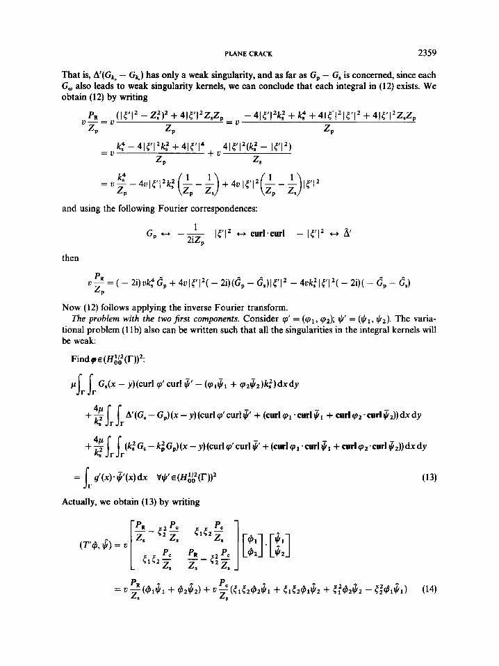
That is, A(G5 - Gk) has only a weak singularity, and as far as G, - G, is concerned, since each G, also leads to weak singularity kernels, we can conclude that each integral in (12) exists. We obtain (12) by writing
PR (1C;’I2 - Z,’)2 + 4)<’J2ZsZp - 41(’l2k,2 + k: + 41t‘121(’12 + 4)<’)2ZsZp u - = u = U
ZP ZP ZP
Z P Z S
k$ - 41t’12kf + 41t’I4 + u41t’12(kf - lr‘I2) = u
and using the following Fourier correspondences:
then
PR ZP
u - = ( - 2i)ukf6, + 4ult’I2( - 2i)(GP - 6s)lt’12 - 4uk,21t’I2( - 2i)( - GP - 6,)
Now (12) follows applying the inverse Fourier transform. The problem with the two Jirst components. Consider cp’ = (ql, q2); +I = ( + 1 , ~j~). The varia-
tional problem (1 lb) also can be written such that all the singularities in the integral kernels will be weak:
Find (rE(H;f(r))’:
pjr jr Gs(x - y)(curl cp‘curl$‘ - (cp1$1 + cp2&)k,Z)dxdy
+ !!!
+$jrlr(k,’G,-k:Gp)(x - y)(curlcp‘curl$’ +(curlcpl *curl$l +c~rlcp~-curl$~))dxdy
A(Gs - G,) (x - y) (curl cp’ curl $’ + (curl cpl - curl 6 + curl cp2 - curl G2)) dx dy k,’ r r
= Jr g’(x)-$‘(x)dx vyE(H;&2(r))2
Actually, we obtain (13) by writing
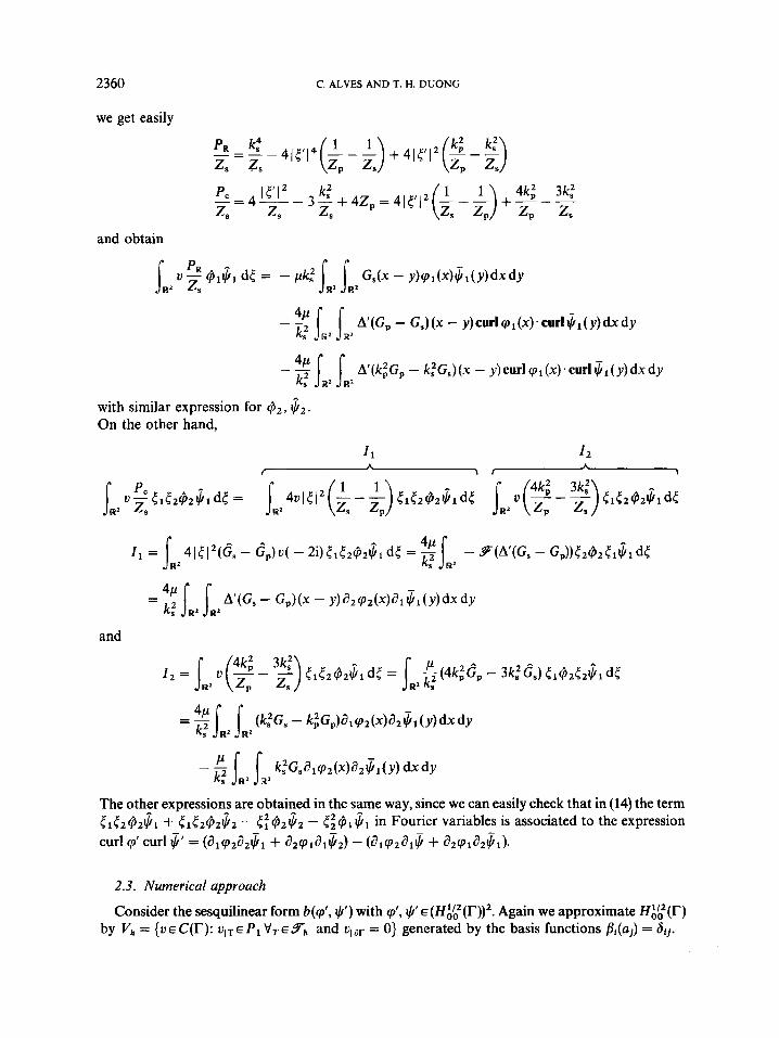
2360
we get easily
C. ALVES AND T. H. DUONG
and obtain
JR2 J GS(x - y)rp,(x)Gl(y)dxdy R'
A(Gp - G,) (x - y ) curl cp (x) . curl ( y) dx dy
A'(kiGp - k:G,)(x - y)curlql(x).curl$,(y)dxdy
with similar expression for &, S2. On the other hand,
L r L f \
and
The other expressions are obtained in the same way, since we can easily check that in (14) the term <1t2@2$1 + 51<2@z$2 - 5:@z$2 - tg@l$l in Fourier variables is associated to the expression curl rp'curl$' = (alrp2a2$1 + a z r p A G 2 ) - (alrp246 + a t ( P d 2 $ 1 ) .
2.3. Numerical approach
Consider the sesquilinear form b(rp', $') with rp', @ E ( H ; f ( r ) ) ' . Again we approximate HtbZ(I') by V,, = (uEC(T): u l T ~ P l VTekTh and UlJr = 0} generated by the basis functions /&(aj) = dij.
PLANE CRACK
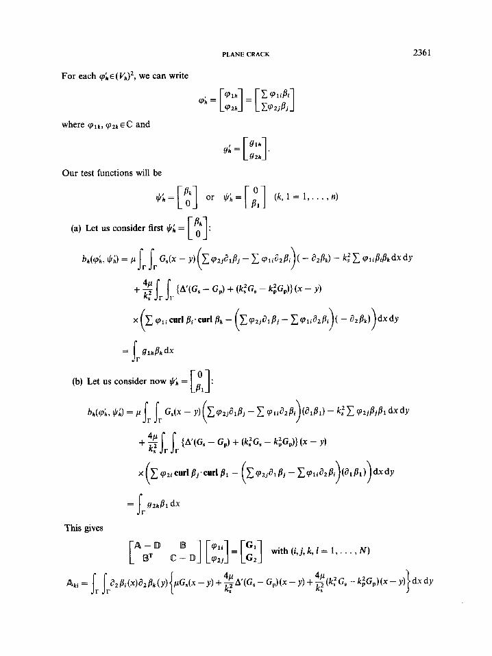
For each q; E (Vh)’, we can write
236 1
Our test functions will be
This gives
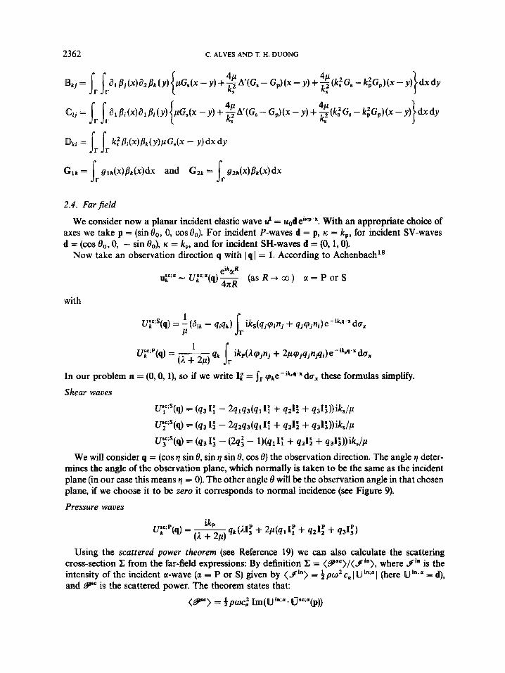
2362 C. ALVES AND T. H. DUONG
2.4. Far field
We consider now a planar incident elastic wave u' = uodeirp.x. With an appropriate choice of axes we take p = (sin d o , 0, cos O0). For incident P-waves d = p, ic = k,, for incident SV-waves d = (cos 8,,, 0, - sin O0), K = k,, and for incident SH-waves d = (0, 1,O).
Now take an observation direction q with lq( = 1. According to Achenbach" eikaR
"y N Q"'"(q) - (asR+oo) a = P o r S 4zR
with
1 uys(q) = -(8ik - q i q k ) iks(qjqinj -t- qj(pjni)e-'k~q'xda,
P lr (A + 2 P ) 4' I ikp(Aqjnj + 2pqjqjnfli)e-'kfl'" do,
us"' P 1 k ' (q) = ___
In our problem n = (O,O, l), so if we write 1; = jr qke-'k*q'Xdo, these formulas simplify.
Shear waves
q%) = (q3I; - 2qlq3(qlI; + q21; + q3I;NikJP
UYS(q) = (43 1; - 24*q3(41It + 4213 + qJI;))iks/P
q S ( q ) = (431; - (24: - l)(qlI; + 421; + 431WkJP We will consider q = (cos q sin 8, sin q sin 0, cos 8) the observation direction. The angle q deter-
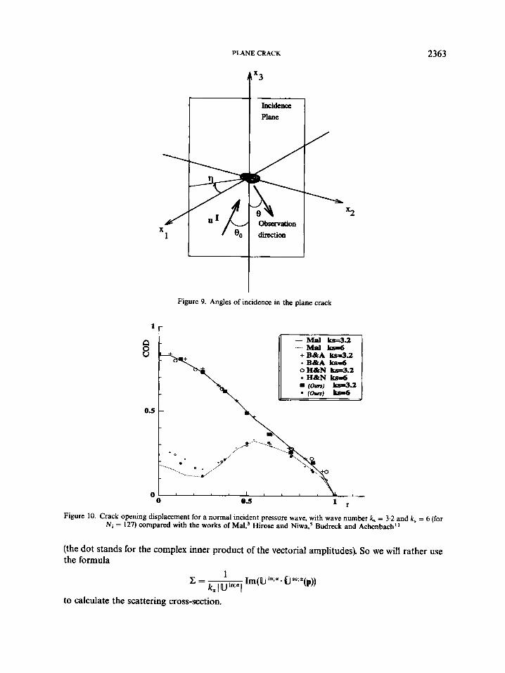
mines the angle of the observation plane, which normally is taken to be the same as the incident plane (in our case this means q = 0). The other angle 8 will be the observation angle in that chosen plane, if we choose it to be zero it corresponds to normal incidence (see Figure 9).
Pressure waves
Using the scattered power theorem (see Reference 19) we can also calculate the scattering cross-section I; from the far-field expressions: By definition I; = (8")/(9'"), where f'" is the intensity of the incident a-wave (a = P or S) given by (3'") = 4 PO' c, I U *";' I (here U'"*' = d), and Pc is the scattered power. The theorem states that:
(9") = fpmc,2 Im(U'";"- Use;'@))
PLANE CRACK 2363
Figure 9. Angles of incidence in the plane crack
1 -
._..__ Mp1
+B&A W . 2 + B&A Lsd oH&N ksd.2 oH&N ksr6
n - 8
0.5 -
0 I , , ,
' r 0 0.5
Figure 10. Crack opening displacement for a normal incident pressure wave, with wave number k, = 3.2 and k. = 6 (for Ni = 127) compared with the works of Mal? Hirose and Niwa,' Budreck and Achenbach"
(the dot stands for the complex inner product of the vectorial amplitudes). So we will rather use the formula
to calculate the scattering cross-section.
2364 C. ALVES AND T. H. DUONG
2.5. Numerical tests.
Tests have been made in order to compare our work with previous ones. This comparison is only possible in special cases of shapes, since the previous works have always been applied to simplified cracks, namely the penny-shaped crack or elliptical cracks. We will focus our comparison in the works of Krenk and Schmidt,16 Martin and Wickham4 and Budreck and Achenbach."
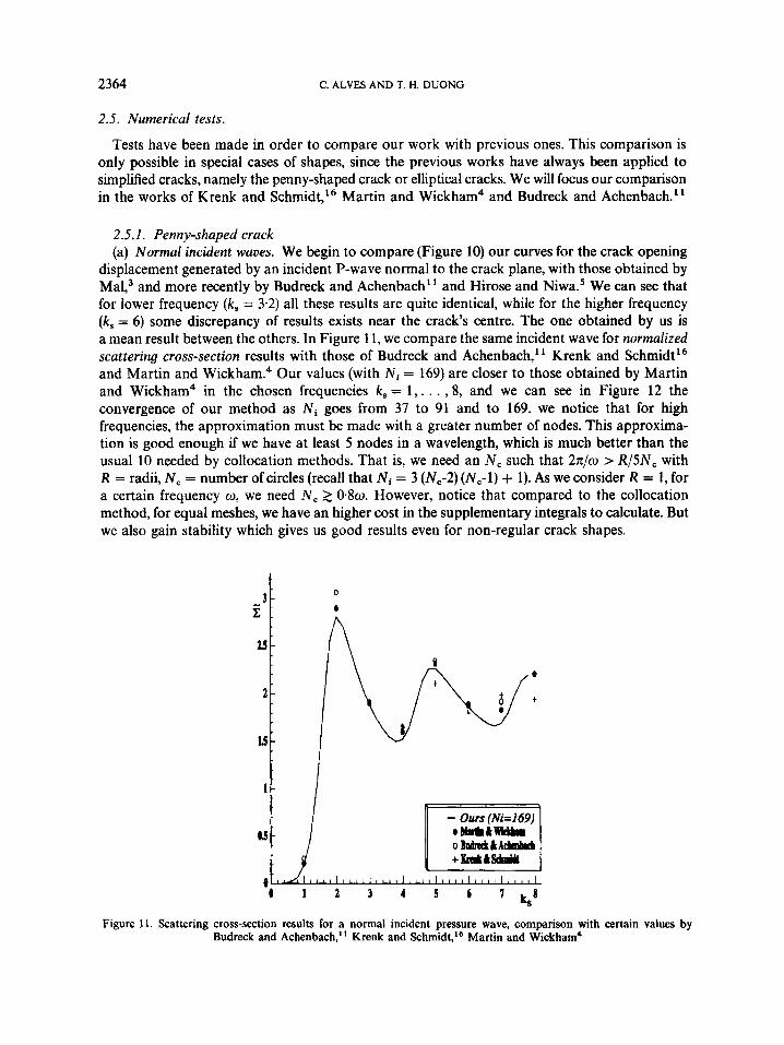
2.5.1. Penny-shaped crack (a) Normal incident waves. We begin to compare (Figure 10) our curves for the crack opening
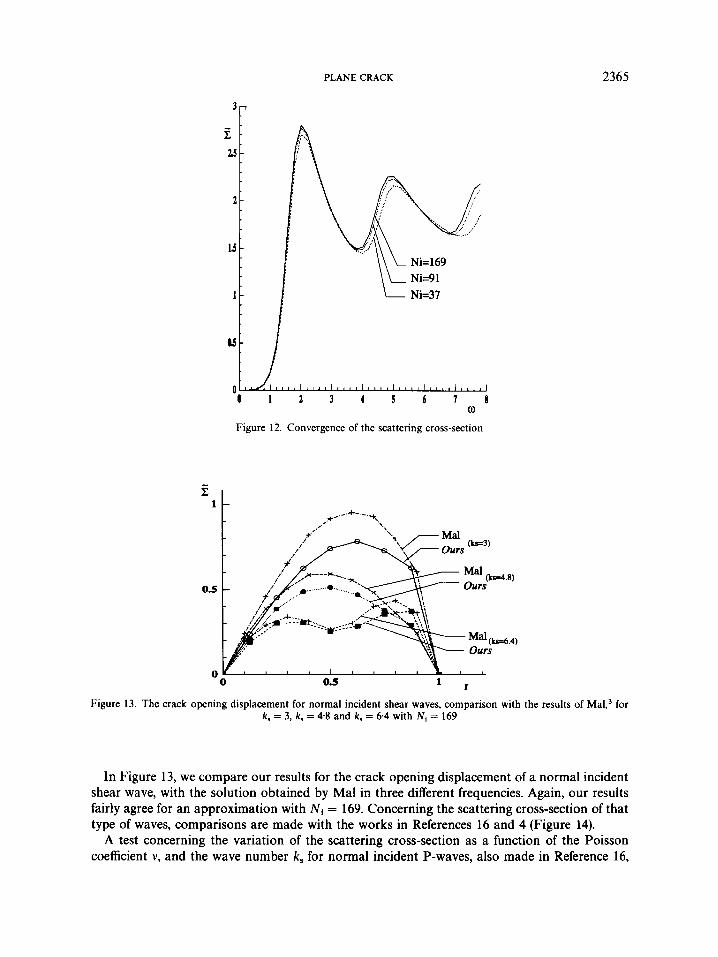
displacement generated by an incident P-wave normal to the crack plane, with those obtained by Mal,3 and more recently by Budreck and Achenbach" and Hirose and Niwa.' We can see that for lower frequency (k, = 3.2) all these results are quite identical, while for the higher frequency (k , = 6) some discrepancy of results exists near the crack's centre. The one obtained by us is a mean result between the others. In Figure 11, we compare the same incident wave for normalized scattering cross-section results with those of Budreck and Achenbach,' ' Krenk and Schmidt16 and Martin and Wickham? Our values (with N i = 169) are closer to those obtained by Martin and Wickham4 in the chosen frequencies k, = 1 , . . . , 8 , and we can see in Figure 12 the convergence of our method as N i goes from 37 to 91 and to 169. we notice that for high frequencies, the approximation must be made with a greater number of nodes. This approxima- tion is good enough if we have at least 5 nodes in a wavelength, which is much better than the usual 10 needed by collocation methods. That is, we need an N , such that 2z/w > R / 5 N , with R = radii, N, = number of circles (recall that Ni = 3 (N,-2) (Nc-l) + 1). As we consider R = 1, for a certain frequency o, we need N , 2 0.80. However, notice that compared to the collocation method, for equal meshes, we have an higher cost in the supplementary integrals to calculate. But we also gain stability which gives us good results even for non-regular crack shapes.
t - 3 - z ; w -
2 -
u-
0
0
- Ours (Ni=169) :I, , , , , , , , , , I , , , , pjiEJ b 1 1 2 3 4 5 1 I Q
Figure 1 1 . Scattering cross-section results for a normal incident pressure wave, comparison with certain values by Budreck and Achenbach," Krenk and Schmidt,I6 Martin and Wickham4
PLANE CRACK 2365
z . ts-
2 -
1s -
1-
0
Figure 12. Convergence of the scattering cross-section
0.5
0 I 0 0.5 ' r
Figure 13. The crack opening displacement for normal incident shear waves, comparison with the results of for k, = 3, k, = 4.8 and k, = 6 4 with Ni = 169
In Figure 13, we compare our results for the crack opening displacement of a normal incident shear wave, with the solution obtained by Ma1 in three different frequencies. Again, our results fairly agree for an approximation with Ni = 169. Concerning the scattering cross-section of that type of waves, comparisons are made with the works in References 16 and 4 (Figure 14).
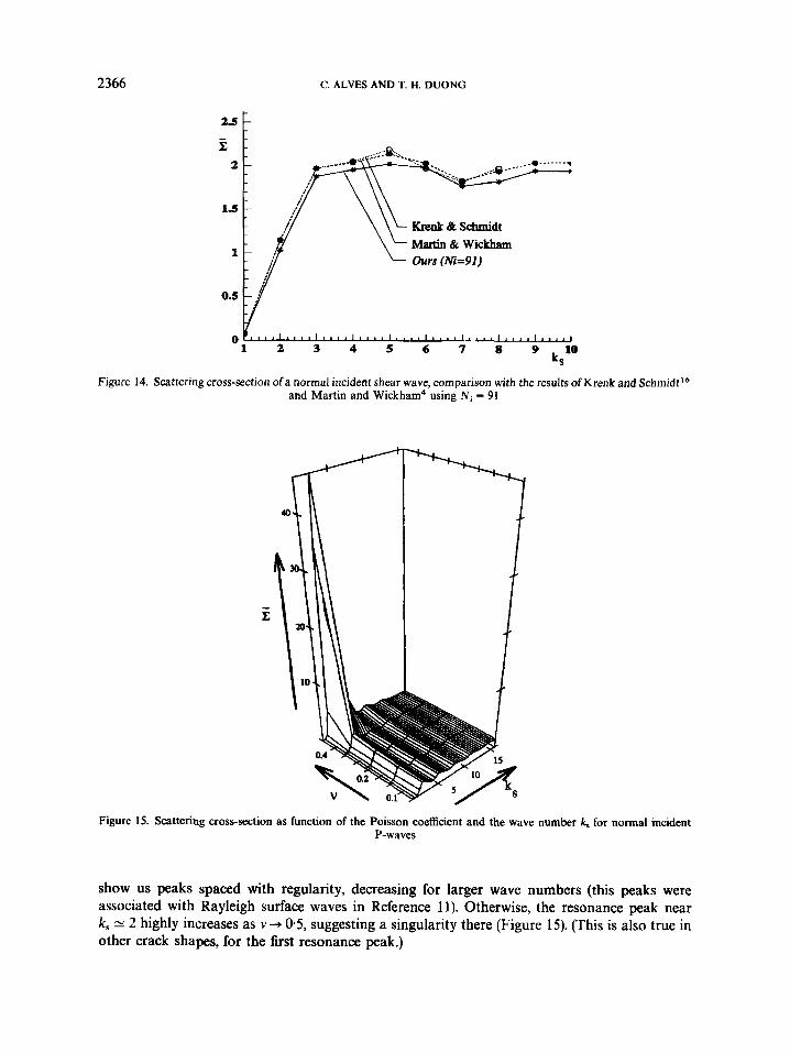
A test concerning the variation of the scattering cross-section as a function of the Poisson coefficient v, and the wave number k, for normal incident P-waves, also made in Reference 16,
2366
2.5 - -
C. ALVES AND T. H. DUONG
L -
Figure 15. Scattering cross-section as function of the Poisson coefficient and the wave number k, for normal incident P-waves
show us peaks spaced with regularity, decreasing for larger wave numbers (this peaks were associated with Rayleigh surface waves in Reference 11). Otherwise, the resonance peak near k, 2: 2 highly increases as v + 0.5, suggesting a singularity there (Figure 15). (This is also true in other crack shapes, for the first resonance peak.)
PLANE CRACK 2367
1-
z -
05- p Krcnk & Schmidt
Oblique Incident W-wave
Wdegrees)
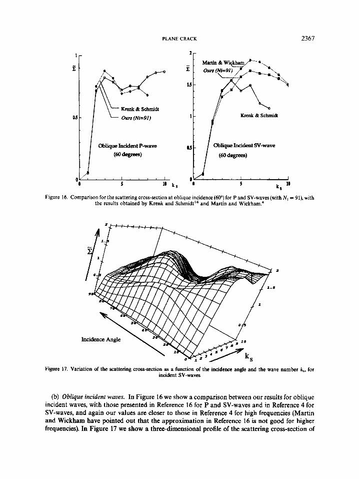
Figure 16. Comparison for the scattering cross-section at oblique incidence (60") for P and SV-waves (with Ni = 91), with the results obtained by Krenk and SchmidtI6 and Martin and Wi~kham.~
3
Incidence Angle
Figure 17. Variation of the scattering cross-section as a function of the incidence angle and the wave number k,, for incident SV-waves
(b) Oblique incident waves. In Figure 16 we show a comparison between our results for oblique incident waves, with those presented in Reference 16 for P and SV-waves and in Reference 4 for SV-waves, and again our values are closer to those in Reference 4 for high frequencies (Martin and Wickham have pointed out that the approximation in Reference 16 is not good for higher frequencies). In Figure 17 we show a three-dimensional profile of the scattering cross-section of
2368 C. ALVES AND T. H. DUONG
t
Incident SV-wave (elastic medium: steel) or,= 10)
, L # , l , , , n l , , , . l
Incidence Angle
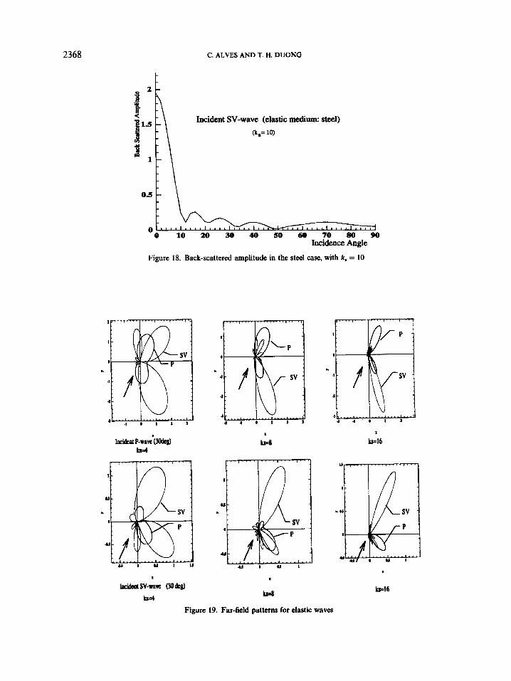
Figure 18. Back-scattered amplitude in the steel case, with k, = 10
0 1 0 2 @ 3 0 4 0 5 0 6 0 7 0 8 0 9 0
b 1 6
Figure 19. Far-field patterns for elastic waves
PLANE CRACK 2369
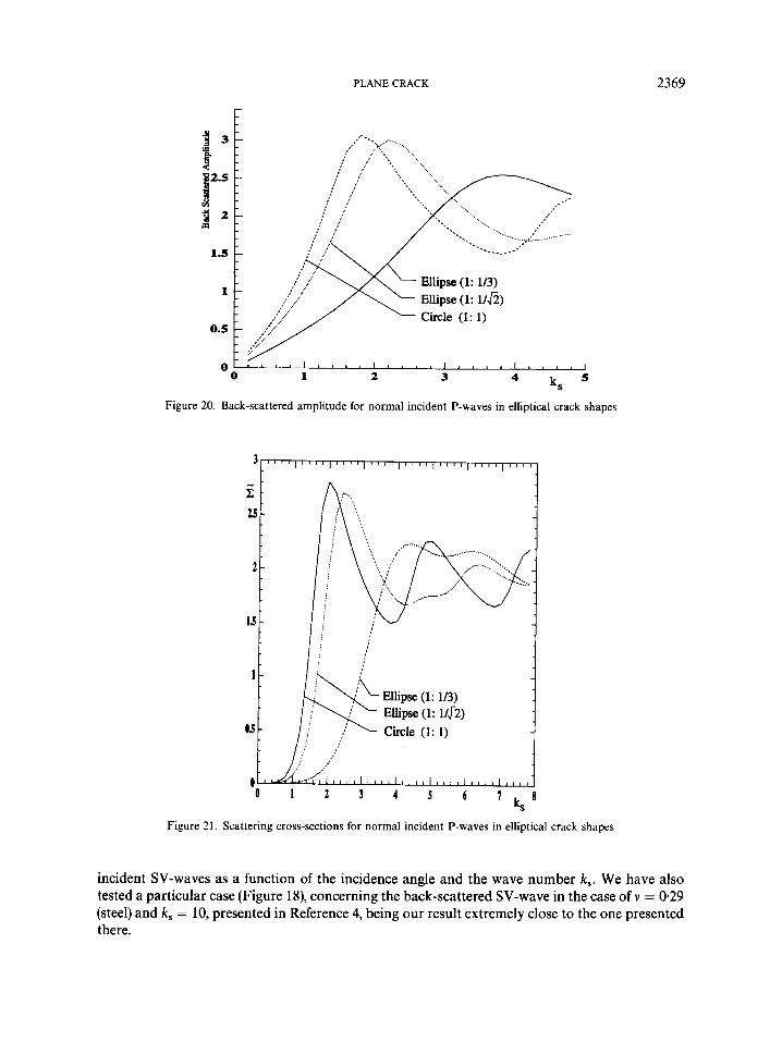
Figure 20. Back-scattered amplitude for normal incident P-waves in elliptical crack shapes
A - . r t z - 25-
2 -
Ellipse (1: 1/3) EIIipse (1: 1/J2)
05 Circle (1: 1) -
1
’ 0 1 2 3 4 5 6
Figure 21. Scattering cross-sections for normal incident P-waves in elliptical crack shapes
incident SV-waves as a function of the incidence angle and the wave number k,. We have also tested a particular case (Figure 18), concerning the back-scattered SV-wave in the case of v = 0.29 (steel) and k , = 10, presented in Reference 4, being our result extremely close to the one presented there.
2370 C. ALVES AND T. H. DUONG
- z : 2 5 -
2 -
Is-
1 -
as- I - Normal Incident P-wave - O6 1 2 3 4 5 6
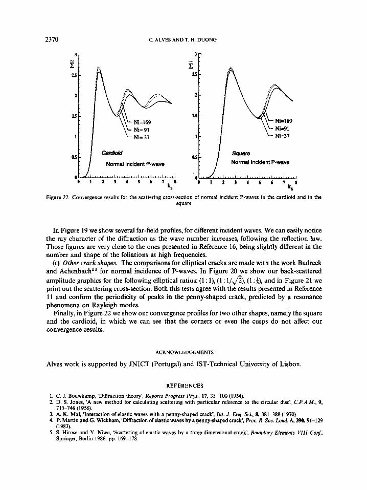
Figure 22. Convergence results for the scattering cross-section of normal incident P-waves in the cardioid and in the square
In Figure 19 we show several far-field profiles, for different incident waves. We can easily notice the ray character of the diffraction as the wave number increases, following the reflection law. Those figures are very close to the ones presented in Reference 16, being slightly different in the number and shape of the foliations at high frequencies.
(c) Other crack shapes. The comparisons for elliptical cracks are made with the work Budreck and Achenbach” for normal incidence of P-waves. In Figure 20 we show our back-scattered amplitude graphics for the following elliptical ratios: (1 : l), (1 : 1/*), (1 :+), and in Figure 21 we print out the scattering cross-section. Both this tests agree with the results presented in Reference 11 and confirm the periodicity of peaks in the penny-shaped crack, predicted by a resonance phenomena on Rayleigh modes.
Finally, in Figure 22 we show our convergence profiles for two other shapes, namely the square and the cardioid, in which we can see that the corners or even the cusps do not affect our convergence results.
ACKNOWLEDGEMENTS
Alves work is supported by JNICT (Portugal) and IST-Technical University of Lisbon.
REFERENCES
1. C. J. Bouwkamp, ‘Diffraction theory’, Reports Progress Phys., 17, 35-100 (1954). 2. D. S. Jones, ‘A new method for calculating scattering with particular reference to the circular disc’, C.P.A.M., 9,
3. A. K. Mal, ‘Interaction of elastic waves with a penny-shaped crack‘, Int. J . Eng. Sci., 8, 381-388 (1970). 4. P. Martin and G. Wickham, ‘Diffraction of elastic waves by a penny-shaped crack‘, Proc. R. Soc. Lond. A, 390,91-129
5. S. Hirose and Y. Niwa, ‘Scattering of elastic waves by a three-dimensional crack’, Boundary Elements VIII Con$,
713-746 (1956).
(1983).
Springer, Berlin 1986, pp. 169-178.
PLANE CRACK 237 1
6. N. Nishimura and S. Kobayashi, ‘Regularised boundary integral method for elastodynamic crack problem’, Cornput.
7. J. C. Nedilec, ‘Curved finite element method for the solution of integral singular equations on surfaces in R”, Comput.
8. A. Bamberger, ‘Approximation de la diffraction d’ondes elastiques (I)’, in Nonlinear Partial Differential Equations and
9. M. A. Hamdi, ‘Une formulation variationnelle par equations integrales pour la resolution de l’equation #Helm-holtz
10. T. Ha Duong, ‘On the boundary integral equations for the crack opening displacement of flat cracks’, Integr. Eq. Oper.
11. D. Budreck and J. Achenbach, ‘Scattering from threedimensional planar cracks by the boundary integral equation
12. W. Lin and L. Keer, ‘Scattering by a planar three-dimensional crack, J. Acoust. SOC. Am., 82, 1442-1448 (1987). 13. C. J. S. Alves, ‘Estudo Matematico e Numeric0 da Difracclo de Ondas Elasticas em Fissuras Planas por um Metodo
14. J. L. Lions and E. Magenes, Non-Homogeneous Boundary Value Problems and Applications, Springer, Berlin, 1972. 15. T. Ha Duong, Thbe de Docteur Ps Sciences, Universite Paris V1, 1987. 16. S. Krenk and H. Schmidt, ‘Elastic wave scattering by a circular crack, Phil. Trans. R. Soc. A, 308, 167-198 (1982). 17. V. D. Kupradze, T. G. Gegelia, M. 0. Basheleishvili and T. V. Burchuladze, Three Dimensional Problems of the
18. J. D. Achenbach, A. K. Gautesen and H. McMaken, ‘Ray methods for waves in elastic solids’, Monog. and Studies in
19. P. J. Barratt and W. D. Collins, ‘The scattering cross section of an obstacle in an elastic solid for plane harmonic
Mech., 4, 319-328 (1989).
Methods Appl. Mech. Eng., 8, 61-80 (1976).
their Applications, Pitman, London, 1984, pp. 48-95.
avec des conditions aux limites mixtes’, CRAS ser. II, 292, 17-20 (1981).
Theory, 15, 426-453 (1992).
method’, J. Appl. Mech., 55, 405-41 1 (1988).
de Equac6es Integrais’, Master Thesis, Universidade de Lisboa, Lisbon, 1992.
Mathematical Theory of Elasticity and Thermoelasticity, North Holland, Amsterdam, 1979.
Mathematics, Vol. 14, Pitman, London, 1982.
waves’, Proc. Camb. Phil. Soc., 61, 969-981 (1965).