northern prairie wetlands and climate change

Northern Prairie Wetlands and Climate Change

Bruce V. Millett1, W. Carter Johnson2, and Richard A. Voldseth3

Departments of Geography1 and Horticulture, Forestry, Landscape, and Parks2

South Dakota State University

Brookings, South Dakota 57007 USA

and

USDA Forest Service3

North Central Research Station

Forest Science Laboratory

Grand Rapids, MN 55744-3399 USA

2

ABSTRACT

The Prairie Pothole Region (PPR) of North America contains millions of wetlands

that provide abundant ecological services that are highly sensitive to climate change. We

explored the broad spatial and temporal patterns across the PPR between climate and

wetland water levels and vegetation by “moving” a wetland model (WETSIM 3.1) among

18 stations with 95-year weather records. Ecoregions were used as the spatial framework

to select weather stations and to compare and contrast model outputs. A critical

component to WETSIM 3.1 was an accurate digital elevation model (DEM) for the

wetland basin. Spatial analysis was performed on model outputs in ArcGIS. Simulations

suggest that optimum wetland conditions would shift under a drier climate from the

center of the PPR (Dakotas and southeastern Saskatchewan) to the wetter eastern and

northern fringes, areas currently less productive and where most wetlands have been

drained.

3

1.0 INTRODUCTION

1.1 Study Area

The Prairie Pothole Region (PPR) of North America covers approximately

715,000 km2 (Euliss et al. 1999), 770,000 km2 (Dahl 1993) or 875,902 km2 (Millett

2004) (Figure 1). It is bounded on the south and southwest by the limits of the

Laurentide ice sheet of the Wisconsinan glaciation and on the west by the ice-marginal

Missouri River. The northern limit of the PPR is the southern boundary of the Canadian

boreal forests of Alberta, Saskatchewan, and Manitoba, and the eastern limit is the

prairie-deciduous forest transition zone. This transition zone shifts eastward when climate

conditions become dry and westward when conditions become wetter (Anderson 1983).

Figure 1. Prairie Pothole Region (PPR) shaded in gray (Omernik 1987, 1995).

4

These wetlands were formed during the Pleistocene Epoch, approximately 18,000

years ago. The mid-continental ice sheets retreated and left behind water filled

depressions called potholes, kettle holes, or sloughs scattered across the landscape. These

prairie wetlands support numerous waterfowl and aquatic plant species. The fossil pollen

record indicates that vegetation of the Great Plains of North America also has undergone

dramatic changes since the Late Pleistocene (Wells 1970).

There are millions of basins within the PPR. Cowardin et al. (1995) estimated that

about 3.1 million wetland basins occur in MN, MT, ND and SD; estimated mean

wetland-basin sizes were 2.7 ha in MN, 1.2 ha in MT, 0.6 ha in ND, and 1.1 ha in SD.

The number of wetlands with water varies from year to year, depending primarily on the

amount of precipitation and runoff. The Canadian Prairie Provinces have between 2 and 7

million wetlands. May pond long-term averages (1961-2001) showed Alberta with

728,000, Manitoba with 1,992,000, and Saskatchewan with 687,000 basins that resulted

in a total of 3.4 million wetlands (Wilkins et al. 2002).

The wetlands of the glaciated prairies of the north central United States and south

central Canada are highly sensitive to weather extremes and changes in climate (Poiani et

al. 1991, Halsey et al. 1997, Hurd et al. 1999, LaBaugh et al. 1996, Meyer et al. 1999,

Fritz et al. 2000, Johnson et al. 2005).

Previous studies focused on a semi-permanent wetland at one location (Poiani et

al. 1991, 1993a, 1993b, 1995, 1996). They developed and used the model WETland

SIMulation (WETSIM) to simulate the vegetation and hydrology in semi-permanent

prairie wetlands. Their results indicated that warmer temperatures, similar to those

5

predicted by various climate models, caused drier conditions, despite increases in

precipitation. The overall result was less open water and greater emergent cover in nine

out of ten climate scenarios. When the cover ratio became unbalanced, either toward

more open water periods or emergent vegetation, productivity of waterfowl declined

(Weller and Spatcher 1965).

This research used a revised version of the simulation model WETland

SIMulation (WETSIM) 3.1, weather data, and analyzed model outputs using Geographic

Information Systems (GIS) to better understand the spatial and temporal sensitivity of

PPR wetlands to climate variability.

1.2 OBLECTIVES

Objective 1. Build accurate Digital Elevation Model (DEM).

An accurate DEM was required for wetland model simulations. A DEM for

bathymetry of Wetland P1 and the surrounding topography of the Cottonwood Lake

study area was created from elevation point data files and required numerous

modifications. The DEM for wetland P1 basin was constructed using the Topogrid model

included in ESRI in ArcGIS 8.1 software. Topogrid generates a hydrologically correct

grid of elevation from point, line and polygon coverages.

Objective 2. Divide the PPR into Ecoregions.

A geographic classification system was sought to define the patterns of ecological

variation across the PPR. Tansley (1935) coined the word "ecosystem" to capture the

regional array of biological and physical forces shaping organisms in nature. The

ecoregion concept is one of the most important in landscape ecology, both for

management and understanding ecological components (Omernik and Bailey 1997,

6

Omernik 1995). Ecological regions are identified through the analysis of the patterns and

the composition of biotic and abiotic phenomena that affect or reflect the differences in

ecosystem quality and integrity (Omernik 1987 and 1995). These often include geology,

hydrology, vegetation, climate, soils, land use, wildlife, and physiography. The relative

importance of each characteristic varies from one ecological region to another regardless

of the hierarchical level (Omernik 1987).

Objective 3. Characterize the historic climate of ecoregions and identify long-term

climate trends across ecoregions.

Weather station data were used to characterize the climate of PPR ecoregions and

for WETSIM 3.1 modeling experiments. Criteria for selecting stations included: their

length of record, and geographic location within an ecoregion. It was important to select

weather stations with long and complete records to accurately represent the weather

throughout the twentieth century. Stations were geographically selected to encompass the

widest range of climatic variation within an ecoregion. Historic normal climate variation

among ecoregions within the PPR was determined from weather station data.

Precipitation and temperature trends were determined from the appropriate 95-year

record from each station.

Objective 4. Develop and use WETSIM 3.1 model outputs in GIS to map areas of

optimum wetland conditions derived from historic and modified climate model

simulations.

The effect of historic and modified climate scenarios on wetland hydrology and

vegetation dynamics was evaluated through simulation of WETSIM 3.1 for the wetland

P1 basin moved among weather stations. Cover ratio and return time were used in

7

WETSIM 3.1 to compare model results across the PPR. The cover ratio is the proportion

of open water to vegetation cover for a wetland. The return time is the length of time for

a wetland to return to a specific phase of the cover cycle.

2.0 DATA AND METHODS

2.1 Brief Description of WETland SIMulation (WETSIM) 3.1

WETSIM 3.1 is a next generation hydrologic model based on WETSIM 2.0

(Poiani and Johnson 1991, 1993a, 1993b, Poiani et al 1995 and 1996). It is a

deterministic model based on watershed and wetland processes. These include watershed

surface processes, watershed groundwater, wetland surface processes, and wetland

vegetation dynamics. The model uses daily precipitation and temperature to calculate

daily wetland water balance, estimate wetland stage, and simulate wetland vegetation

from May through September. Model simulations used weather station data for each

ecoregion. Model parameters that varied geographically among weather stations were

maximum temperature, minimum temperature, precipitation, initial starting volume, and

latitude.

The WETSIM 3.1 vegetation sub-model calculated spatial distribution of

vegetation cover types and open water in the wetland. A grid of uniform cells represented

the wetland and upland margin. Cell size for initial model simulations was 25 m2. The

elevation data used in the hydrology sub-model were applied to simulate vegetation

dynamics. Calibration stage levels were provided by Tom Winter, USGS.

8

The approach used in this study was to “move” the P1 model wetland to each of

the 18 weather stations to examine the effect of climate variation on wetland processes.

In effect, this approach “excised” the P1 watershed and all of its characteristics (soils,

topography, upland vegetation) and subjected it to the full range of PPR climates.

Cover ratio and return time were two indices developed for the WETSIM 3.1

output to determine optimum wetland conditions. Wetland cover ratio conditions were

divided into three categories; closed marsh phase (0 to 25 percent open water), hemi-

marsh phase (>25 to <75 percent open water), and open-water phase (>75 percent open

water). The return time represents the length of time for a wetland to return to a specific

phase of the cover cycle. This value was determined by the number of times the model

wetland completed the cover cycle during the 95-year simulations at each weather

station.

2.2 Prairie Wetland Ecoregion Boundary Delineation

The method used to delineate ecoregions was based on the premise that ecological

regions can be identified through the analysis of patterns of biotic and abiotic phenomena

that reflect differences in ecosystem quality and integrity (Wilken 1986, Omernik 1987,

1995). Level I and Level II divide the North American continent into 15 and 51 regions,

respectively. At Level III, the continental United States contains 98 regions (United

States Environmental Protection Agency [USEPA] 1996). Level IV regions are more

detailed ecoregions for state level applications; Level V regions are the most detailed and

used for landscape-level or local-level projects.

9

Canada uses a similar hierarchical approach for delineating ecoregions. It has 15

ecozones, 53 terrestrial ecoprovinces, 194 ecoregions, and 1021 ecodistricts (Marshall

and Schut 1999). The prairie ecozone delineates the Canadian portion of the PPR. In

1991 a collaborative project was undertaken by a number of federal agencies in

cooperation with provincial and territorial governments, all under the auspices of the

Ecological Stratification Working Group. The working group focused on three priority

levels of stratification: ecozones, ecoregions, and ecodistricts (Ecological Stratification

Working Group 1996). The Canadian ecoregions tended to be more finely defined than

the U.S. ecoregions at the same level. The prairie ecozone was divided into nine

ecoregions.

A relatively small number of ecoregions was sought because the analysis planned

for each ecoregion required a large amount of climate data. The US Level IV ecoregions

and Canadian ecodistricts provided the most detail with 198 subregions (Figure 2A).

Some of these could be merged at the US-Canadian border. However, due to the large

number of divisions, it was impractical for the scope of this project to use this many

subdivisions. The Level III ecoregions provided only four large ecoregions, referred to as

the Lake Agassiz Plain, Mixed Grassland, Moist Mixed Grassland, and Western Corn

Belt Plains. In addition these were a few small regions near the Cypress Hills that border

Alberta and Saskatchewan and the isolated peaks near the foothills of the Rocky

Mountains (Figure 2B). Since these relatively small areas were not to be a focus of this

study, they were incorporated into the much larger ecoregion that surrounded them.

Further subdivision was still sought to show more physiographic detail within the PPR.

Two more ecoregions were defined. The first was an important physical feature called the

10

B C

PRAIRIE POTHOLE REGIONECOREGIONS

A

Figure 2 A. PPR US Level IV ecoregions and Canadian ecodistricts form 358 subregions. B. PPR Level III ecoregions are the Lake Agassiz Plain, Mixed Grassland, Moist Mixed Grassland, and Western Corn Belt Plains. C. Modified version of PPR ecoregions with the Prairie Coteau and Aspen Parkland added to the Level III ecoregions. 2.3 Weather Station Data Selection and Preparation

Prairie Coteau located in eastern South Dakota and southwestern Minnesota. The second

division was the Canadian Aspen Forests and Parklands, which forms an arc along the

northern portion of the PPR (Figure 2C). This ecoregion represents the transition between

the boreal forest to the north and the grasslands to the south. It is characterized by aspen,

oak groves, mixed tall shrubs, and grasslands.

11

Three weather stations were selected to characterize the climate of each

ecoregion, comprising 18 total stations. These stations were chosen based on their

longevity of record, geographic location within each ecoregion, and completeness of

record. Records of 95 years were desired to encompass the widest range of climatic

variation. For example, most ecoregions in the PPR have a north-south orientation, thus

weather stations were selected from northern, central, and southern locations to represent

this environmental gradient. A GIS database for the PPR was created to facilitate weather

station selection. The database contained station latitude, longitude, elevation, and the

start and end data collection dates. The widest separation of stations was sought to

provide the most complete representation for the ecoregion, while maintaining those

stations with long records. Weather stations with at least some temperature and

precipitation data prior to 1932 are highlighted in yellow (Figure 3). All weather stations

had at least some breaks in their period of record. Some stations collected only partial

weather data such as temperature and then collected precipitation many years later. Other

stations may have collected data only seasonally with little or no data during the winter

months. Another common problem involved long gaps in the data record. These were

stations where collection was interrupted for several months or years before recording

resumed. Missing data were replaced by extrapolating from three nearby stations where

possible. Occasionally one or two stations were used for extrapolation when there were

no stations nearby with data during the missing data period. It was more common to find

only one nearby station during the early part of the twentieth century because there were

fewer stations collecting data.

12

Figure 3. Weather stations with data records prior to 1932 are highlighted in yellow.

The large climate datasets were managed using Microsoft EXCEL and ArcView

software. They were reduced to three variables: daily precipitation, maximum daily

temperature, and minimum daily temperature. Missing records, in the actual columns

were designated as –99999, and replaced with estimated values. Data files were checked

for outliers. After all the –99999 (missing data) and erroneous data were replaced with

the estimated values, the table was exported to a tab delimited text file. Files from some

of these weather stations exceeded 100 years but it was more desirable to trim these

datasets to 95 years so they were all of equal size.

13

The input format for WETSIM 3.1 required columns for years, months, days,

precipitation, minimum daily temperature, and maximum daily temperature. The United

States weather station temperatures were then converted in Excel to degrees Celsius and

precipitation records were converted to millimeters. Each of the 18 weather stations had

34,699 records for the 95 years of daily weather data. The total number of records for

daily precipitation, maximum daily temperature, and minimum daily temperature resulted

in 104,097 records for each weather station. The total for all elements and stations was

1,873,746 records to use as inputs to WETSIM 3.1 and to use in the analysis of weather

trends.

2.4 Digital Elevation Model (DEM)

2.4.1 Point Data Preparation

The semi-permanent wetland chosen to model was the Wetland P1 located at the

Cottonwood Lake study area, Stutsman County, North Dakota (Figure 4). A DEM for

bathymetry of Wetland P1and the surrounding topography of the Cottonwood Lake study

area was created in the following way. Elevation point data files were provided by Tom

Winter (U. S. Geological Survey). These raw data files required numerous modifications

before they could be used in GIS applications. Normally the first step would involve

converting the format of the .dig files into ARC/INFO coverage’s, but this could not be

accomplished because each file contained points that were in a Cartesian coordinate

system and there were no geographic coordinates to use for a reference. This meant that

each point was positioned correctly in relation to the other points but the points needed to

be transformed into a geographic coordinate system.

14

There were 117 small files containing 87,031 points. These small files of

elevation point data were put together into a single large file. Point data were extracted

from the files and put into a Microsoft EXCEL file. The data entered into EXCEL

consisted of the X coordinate, Y coordinate, Z value (elevation), and unique

identification number for each point. Data were added until they reached the limit of

EXCEL’s row capacity of 65,000. Another EXCEL file was created for the remaining

points. The EXCEL files were then saved as tab delimited text files. These text files were

imported into ArcView assigning the X and Y coordinates appropriately. The file was

then converted into a shapefile and then into ARC/INFO coverage.

Elevation contours were interpolated from the point data and overlaid onto a

Digital Raster Graphic (DRG) and a Digital Orthophoto Quadrangle (DOQ). A DRG is a

scanned image of a U.S. Geological Survey (USGS) standard series topographic map,

including all map collar information. The image inside the map neatline is georeferenced

to the surface of the earth and fit to the Universal Transverse Mercator projection. A

DOQ is a uniform-scale aerial photograph. It is georeferenced and is able to serve as a

base map on which other map information may be overlaid. The DRG and DOQ were

used as a visual reference to position the survey contours. Positioning the contours

required numerous trial and error steps until a best fit was found. Once this step was

completed a point file was then geographically registered in Universal Transverse

Mercator (UTM) North American Datum 1983. These data were then used to construct

the DEM.

15

P8

P2

P1

P6

P4/P5

P7

P9

T2

P3

T3T1

T5

T6T4

5

573

570

56

564558

552

555

564

564

567

570

564

564

576

5

561

570564

564

573

561

570

558567

558

558

5 70

558

570

558

561

561

561

564

561

558

576

567

561

567579

567

579

564570

567

567

567

567

55 8

Elevation551 - 552552 - 554554 - 555555 - 557557 - 559559 - 560560 - 562562 - 563563 - 565565 - 566566 - 568568 - 570570 - 571571 - 573573 - 574574 - 576576 - 577577 - 579579 - 581581 - 582No Data

WETLANDS

50 0 50 100 150 200 Meters

N

EW

S

Cottonwood LakeStudy AreaP1 Wetland

#

Figure 4. Cottonwood Lake study area is located in Stutsman County, North Dakota. Wetland P1 is located in the south-central portion of the study area.

2.4.2 DEM Construction

The PPR is a difficult area to map for hydrological purposes because many areas

do not have a functional surface drainage network. The landscape is dotted with small

depressions that require very detailed elevation surveys. Some of these water-filled

16

depressions may or may not be hydrologically connected at the surface. In many

instances these wetlands have subsurface connections via the water table.

The DEM for wetland P1 basin was constructed using the Topogrid model

included in ESRI in ArcGIS 8.1 software. Topogrid generates a hydrologically correct

grid of elevation from point, line and polygon coverages. The Topogrid command is an

interpolation method specifically designed for the creation of hydrologically correct

digital elevation models (DEMs) from comparatively small, but well selected elevation

and stream coverages. It is based upon the ANUDEM program developed by Michael

Hutchinson (1988, 1989).

Construction of a DEM was needed to support the vegetation dynamics portion of

the WETSIM 3.1 model. A 5x5-meter grid was created for the P1 wetland basin using

Topogrid. The program imposes a global drainage condition that automatically removes

most errors in the data. However, the DEM required numerous modifications, these

included the removal of spurious peaks and sinks. There were several topographic

anomalies within the bottom of the basin that resulted from limited bathymetric data.

Points were added to adjust the elevation values and to remove problematic peaks and

sinks.

2.4.3 Watershed delineation

Drainage boundaries may be delineated manually from a topographic map,

digitized from Digital Raster Graphic map (DRG), or determined through the use of

raster data from Digital Elevation Models. An early version of Arc Hydro tools for

ArcView 3.3 was used to derive several data sets to describe the drainage patterns of the

17

watershed from the P1 semi-permanent wetland DEM. Raster analysis was performed to

generate data on flow direction, flow accumulation, stream definition, stream

segmentation, and watershed delineation.

Three wetlands are contained in the P1 semi-permanent watershed: P1, T1, and

T3. T1 and T3 wetlands coalesce with P1 at high stage levels. Temporary wetland T1

along with semi-permanent wetland P1 form a single wetland when the water level is

above an elevation of 558.5 meters or when water depth exceeds 0.8 meters. This study

used the combined watersheds of T1 and P1 as the base watershed. There were two pour

points used to determine two watersheds. A pour point is the point at which water flows

out of an area. It is the lowest point along the boundary of a drainage basin. The first pour

point was used to calculate the P1 semi-permanent wetland and T1 temporary wetland

watershed. A second pour point was positioned between T3 temporary wetland and P1

semi-permanent wetland. At an elevation 559.65 meters or at water depth of

approximately 1.65 meters the ponds coalesce. The location of the pour points was

determined by creating contour lines from the DEM and finding the lowest elevation that

would allow for water to escape in the event that the basin were to fill with water. The

area of the watershed for P1 semi-permanent wetland is 163,383 m2 and the T3 watershed

is 57,866 m2 (Figure 5).

18

Figure 5. P1 and T3 watershed areas.

3.0 RESULTS

3.1 Ecoregion Delineation

The classification process resulted in six modified level III ecoregions (Figure 6).

The Canadian Aspen Forests and Parklands ecoregion extends in a broad arc from

southwestern Manitoba, northwestward through Saskatchewan to its northern limit in

central Alberta. The parkland is a transitional region between the boreal forest to the

north and the grasslands to the south. The Central Tall Grasslands was once covered with

19

Figure 6. Six ecoregions and 18 selected weather stations for the PPR.

tallgrass prairie; more than 75 percent of the region is now used for cropland agriculture

and much of the remainder is in forage for livestock. The landscape varies from nearly

level to gently rolling glaciated till plains and hilly loess plains. The Northern Mixed

Grasslands comprises the northern extension of open grasslands in the Interior Plains of

Canada and extends southward into the Dakotas. The Northern Short Grasslands is a

semiarid grassland ecoregion in southwestern Saskatchewan, southeastern Alberta,

northern Montana and central Dakotas. The Northern Tall Grasslands was formed by

Glacial Lake Agassiz. It produced an extremely flat landscape with beds of lake

sediments on top of glacial till. In the U.S. this region is known as the Red River Valley

and in Canada it is called the Lake Manitoba Plain. The Prairie Coteau is the result of

stagnant glacial ice melting beneath a sediment layer. The hummocky landscape has

20

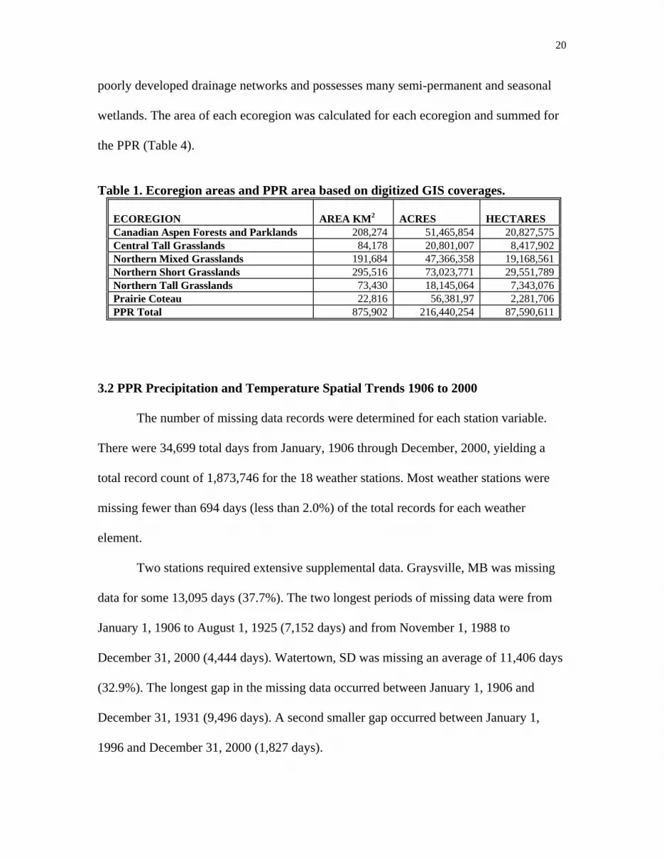
poorly developed drainage networks and possesses many semi-permanent and seasonal

wetlands. The area of each ecoregion was calculated for each ecoregion and summed for

the PPR (Table 4).

Table 1. Ecoregion areas and PPR area based on digitized GIS coverages.

ECOREGION AREA KM2 ACRES HECTARES Canadian Aspen Forests and Parklands 208,274 51,465,854 20,827,575Central Tall Grasslands 84,178 20,801,007 8,417,902Northern Mixed Grasslands 191,684 47,366,358 19,168,561Northern Short Grasslands 295,516 73,023,771 29,551,789Northern Tall Grasslands 73,430 18,145,064 7,343,076Prairie Coteau 22,816 56,381,97 2,281,706PPR Total 875,902 216,440,254 87,590,611

3.2 PPR Precipitation and Temperature Spatial Trends 1906 to 2000

The number of missing data records were determined for each station variable.

There were 34,699 total days from January, 1906 through December, 2000, yielding a

total record count of 1,873,746 for the 18 weather stations. Most weather stations were

missing fewer than 694 days (less than 2.0%) of the total records for each weather

element.

Two stations required extensive supplemental data. Graysville, MB was missing

data for some 13,095 days (37.7%). The two longest periods of missing data were from

January 1, 1906 to August 1, 1925 (7,152 days) and from November 1, 1988 to

December 31, 2000 (4,444 days). Watertown, SD was missing an average of 11,406 days

(32.9%). The longest gap in the missing data occurred between January 1, 1906 and

December 31, 1931 (9,496 days). A second smaller gap occurred between January 1,

1996 and December 31, 2000 (1,827 days).

21

Precipitation and temperature trends varied across the PPR (Figure 7). Three areas

that became drier occurred in the northwestern, central, and southeastern portion of the

PPR. Areas of increased precipitation surrounded these drier regions. Precipitation at

eastern stations tended to increase more than western stations. The statistical results

indicated that the areas on the map ranging from green to lighter blue were not

statistically significant. Dark blue indicated areas with the greatest increases in

precipitation and were statistically significant.

The greatest increase in minimum temperatures occurred in the central and

northern portions of the PPR (Figure 7). Maximum temperature increased in the west

central and northeastern portions of the PPR. Cooling occurred in the southern and very

western PPR. Northern stations tended to warm more than southern stations for both

minimum and maximum temperatures. Statistical analysis indicated that the mid

spectrum colors (Figure 7) for temperatures (green-light yellow range) were not

statistically significant. However, the bolder colors (blue and bright yellow – red) were

significant.

22

Figure 7. Historic precipitation, minimum and maximum daily temperature trends for the Prairie Pothole Region from 1906-2001. Graphs illustrate longitudinal gradient for precipitation trend and latitudinal gradient for minimum and maximum temperature trends.

23

3.3 Optimum Wetland

Historic and climate change simulations were mapped and shaded to show areas

with >30% hemi-marsh conditions and the occurrence of at least one return time during

the 95-year period. These conditions represented optimum wetland conditions (Figure 8).

Prairie Pothole Region Optimum Wetland Conditions

HISTORIC

Figure 8. Shaded areas represent at least one return time and hemi-marsh conditions occurring greater than 30% of the 95-year period from 1906 to 2000. Results are based on six weather stations: Algona, IA, Crookston, MN, Medicine Hat, AB, Minot, ND, Muenster, SK, and Watertown, SD. Hemi-marsh conditions were classified as >25% and <75% vegetation cover.

Optimum wetland conditions shifted geographically as climate was varied. The

historic simulation showed that at least a portion of all six ecoregions experienced

24

optimum wetland conditions during the 95-year simulations. The temperature +3oC

simulation shifted optimum conditions northward and eastward and eliminated the

optimum conditions in the Northern Mixed Grasslands, Northern Short Grasslands, and

almost all of the Canadian Aspen Forests and Parklands (Figure 9).


TEMPERATURE +3C


The precipitation -20%/ temperature +3oC simulation posed the greatest threat to

optimum semi-permanent wetland conditions. The southern Central Tall Grasslands was

the only area of the PPR to exhibit optimum conditions (Figure 10).

25


PRECIPITATION -20% TEMPERATURE +3C


Future climate changes will affect wetlands in two fundamental ways: the number

of functioning wetlands within most ecoregions will decline and the geographic location

of optimum wetlands will shift. Wetland simulations in this study indicated that the

Northern Short Grasslands were the most vulnerable portion of the PPR to increases in

temperature. Semi-permanent wetlands in this ecoregion have historically functioned on

the margin, and any increase in temperature would result in decreases in water levels and

increases in vegetation cover. The central portion of the PPR is currently the most

26

ecologically diverse and productive. Model simulations indicate that this area could shift

eastward and northward with warmer temperatures, although precipitation increases

would offset this shift. The least vulnerable areas were the eastern and southeastern

portions of the PPR. These areas currently have stable wetlands. Warmer temperatures

would tend to improve wetland conditions. Wetlands in this region currently function

more like lakes.

Prairie wetlands have been shown to be very sensitive to climate change. They

have also proven their ability to adapt to the wide variety of weather extremes that occur

within the PPR. As climate continues to change the boundaries of the PPR and its

associated ecoregions will to shift to new locations. The shift in optimum wetland

conditions will reduce the number of existing prairie wetlands. Semi-permanent wetlands

functioning on the margins of the PPR would be the most vulnerable to climate change.

Wetlands in the western portion of the PPR would be more vulnerable to warming

temperatures and lower rainfall. This study showed that only a small portion of the PPR

would benefit from warming temperatures and lower rainfall.

27

ACKNOWLEDGMENTS

This research was supported by grants from the U. S. Environmental Protection Agency

(Habitat and Biological Diversity Research Program) and the U. S. Geological Survey

(Biological Resources Division’s Global Change Research Program). Rosemary Carroll

and John Tracy of the Desert Research Institute in Reno, NV provided groundwater

equations for wetland P1. Tom Winter of the U. S. Geological Survey generously

provided water level and topographic data for wetland P1. We acknowledge the

pioneering work of Karen Poiani of The Nature Conservancy in prairie wetland

modeling, and George Swanson of the Northern Prairie Wildlife Research Center and

Tom Winter for their vision in establishing a long-term monitoring program at

Cottonwood Lake. Twentieth century weather data were collected from the National

Climate Data Center (NCDC), National Oceanic and Atmospheric Administration

(NOAA), U.S. Department of Commerce and the Environment Canada (EC) Manitoba

and Arctic.

28

REFERENCES

Anderson, R. C. 1983. The Eastern Prairie-Forest Transition: An Overview. In: Brewer,

Richard, ed. Proceedings, 8th North American Prairie Conference; 1982 August

1-4; Kalamazoo, MI. Kalamazoo, MI: Western Michigan University, Department

of Biology: 86-92.

Cowardin, L. M., Terry L. Shaffer, and Phillip M. Arnold. 1995. Evaluations of duck

habitat and estimation of duck population sizes with a remote-sensing-based

system. National Biological Service, Biological Science Report 2. Jamestown,

ND: Northern Prairie Wildlife Research Center Home Page.

http://www.npwrc.usgs.gov/resource/othrdata/duckhab/duckhab.htm

(Version 16JUL97).

Dahl, T. E., 1993. Wetland drainage and restoration potential in the Lake Thompson

watershed, South Dakota, USA. In Towards the Wise Use of Wetlands. Ed. Davis,

T. J. <http://www.ramsar.org/lib/lib_wise.htm#cs15 > (21 December 2005).

Ecological Stratification Working Group. 1996. A National Ecological Framework for

Canada. Agriculture and Agri-Food Canada, Research Branch, Centre for Land

and Biological Resources Research and Environment Canada, State of

Environment Directorate, Ottawa/Hull. 125pp. And Map at scale 1:7.5 million.

Pdf copy available from </cansis/publications/ecostrat/intro.html>

Euliss, N. H., Jr., D. M. Mushet, and D. A. Wrubleski. 1999. Wetlands of the Prairie

Pothole Region: Invertebrate Species Composition, Ecology, and Management.

Pp. 471-514 in D. P. Batzer, R. B. Rader and S. A. Wissinger, eds. Invertebrates

29

in Freshwater Wetlands of North America: Ecology and Management, Chapter

21. John Wiley & Sons, New York. Jamestown, ND: Northern Prairie Wildlife

Research Center Home Page.

http://www.npwrc.usgs.gov/resource/1999/pothole/pothole.htm (Version

02SEP99).

Fritz, S. C., E. Ito, Z. Yu, K. R. Laird, and D. Engstrom. 2000. Hydrologic variation in

the northern Great Plains during the last two milennia. Quaternary Research.

53: 175-184.

Halsey, L., D. Vitt, and S. Zoltai. 1997. Climatic and physiographic controls on wetland

type and distribution in Manitoba, Canada. Wetlands. 17:2 243-262.

Hurd, B., N. Leary, R. Jones, and J. Smith. Relative vulnerability of water resources to

climate change. 1999. Journal of the American Water Resources Association.

35:6 1399-1409.

Hutchinson, M. F. 1988. Calculation of hydrologically sound digital elevation models.

Third International Symposium on Spatial Data Handling, Sydney. Columbus,

Ohio: International Geographical Union.

_____. 1989. A new procedure for gridding elevation and stream line data with automatic

removal of spurious pits. Journal of Hydrology.106, 211-232.

Johnson, W. C., B. V. Millett, T. Gilmanov, R. A. Voldseth, G. R. Guntenspergen, and D.

E. Naugle. 2005. Vulnerability of northern prairie wetlands to climate change.

Bioscience. 55:10 863-872.

Labaugh, J. W., T. C. Winter, G. A. Swanson, D. O. Rosenberry, R. D. Nelson, and N. H.

Euliss Jr. 1996. Changes in atmospheric circulation patterns affect mid-continent

30

wetlands sensitive to climate. Limnology and Oceanography. 41:15 864-870.

Marshall I. B. and P. H. Schut. 1999. A National Ecological Framework for Canada –

Overview. A cooperative product by Ecosystems Science Directorate,

Environment Canada and Research Branch, Agriculture and Agri-Food Canada.

http://sis.agr.gc.ca/cansis/nsdb/ecostrat/intro.html.

Meyer, J. L., M. J. Sale, P. J. Mulholland, and N. L. Poff. 1999. Impacts of climate

change on aquatic ecosystem functioning and health. Journal of the American

Water Resources Association. 35:6 1373-1386.

Millett, B. V. 2004. Vulnerability of Northern Prairie Wetlands to Climate Change.

Ph.D. Dissertation. South Dakota State University. Brookings, SD.

Omernik, J. M. 1987. Ecoregions of the Conterminous United States. Annals of the

Association of American Geographers. 77(1): 118-125.

_____. 1995. Ecoregions: A framework for environmental management. In: Biological

Assessment and Criteria: Tools for Water Resource Planning and Decision

Making. W. Davis and T. Simon (eds.). Chelsea, MI: Lewis Publishers.

Poiani, K. A., and W.C. Johnson. 1991. Global warming and prairie wetlands: Potential

consequences for waterfowl habitat. BioScience 41(9): 611-618.

Poiani, K. A., and W. C. Johnson, 1993a. Potential effects of climate change in a semi-

permanent prairie wetland. Climatic Change 24: 213-232.

Poiani, K. A., and W. C. Johnson. 1993b. A spatial simulation model of hydrology and

vegetation dynamics in semi-permanent prairie wetlands. Ecological Applications

3: 279-293.

Poiani, K. A., W. C. Johnson, and T.G.F. Kittel. 1995. Sensitivity of a prairie wetland to

31

increased temperature and seasonal precipitation changes. Water Resources

Bulletin 31:2 283-294.

Poiani, K. A., W. C. Johnson, G. A. Swanson, and T. C. Winter. 1996. Climate change

and northern prairie wetlands: simulations of long-term dynamics. Limnology and

Oceanography 41:5 871-881.

Tansley, A. G. 1935. The use and abuse of vegetational concepts and terms. Ecology

16: 284-307.

U.S. Environmental Protection Agency (USEPA). 1996. Level III Ecoregions of the

Continental United States (revision of Omernik, 1987). Corvallis, Oregon, U.S.

Environmental Protection Agency - National Health and Environmental Effects

Research Laboratory Map M- 1, various scales.

Weller, M. W. and C. E. Spatcher. 1965. Role of Habitat in the Distribution and

Abundance of Marsh Birds. Iowa State University. Agric. & Home Econ. Exp.

Sta. Spec. Rep. No. 43. 31.

Wells, P. V. 1970. Postglacial vegetational history of the Great Plains. Science. 167:

1574-1582.

Wiken, E. B. 1986. Terrestrial Ecozones of Canada. Ecological Land Classification,

Series No. 19. Environment Canada. Hull, Quebec. 26pp. + map.

Wilkens, K. A. and M. C. Otto. 2002. Trends in Duck Breeding Populations, 1955-2002.

U.S. Fish and Wildlife Service, Division of Migratory Bird Management.

Administrative Report. Jul 3.

northern prairie wetlands and climate change

Documents