nonoptimality of the friedman rule with capital income taxation

ALBERTO PETRUCCI

Nonoptimality of the Friedman Rule with Capital

Income Taxation

This paper studies the efficient taxation of money and factor income inintertemporal optimizing growth models with infinite horizons, transactioncosts technologies, and flexible prices. Second-best optimality calls for apositive inflation tax and a nonzero capital income tax when there are re-strictions on taxation of production factors or profits/rents. Our cases ofnonoptimality of the Friedman rule—which differ from those of Mulliganand Sala-i-Martin (1997) and extend substantially those of Schmitt-Groheand Uribe (2004a)—follow from the violation of the Diamond and Mirrlees(1971) principle on production efficiency.

JEL codes: E31, E52, E61, E63, O41Keywords: optimal inflation tax, factor taxation, transaction costs technology,

second-best analysis, capital accumulation.

SHOULD MONEY BE exempted from taxation? Initially, two con-trasting answers were given to this question. One was provided by Friedman (1969),who claimed, from a normative standpoint, that the inflation tax—the nominal interestrate—should be brought to zero when lump-sum taxes are available. Money shouldbe tax free because the marginal private cost of holding money (i.e., the nominalinterest rate) should be equated to the marginal social cost of money, which is zeroas money is costless to produce. The Friedman rule is a first-best monetary policyprescription obtained in a partial equilibrium setup.

A second answer was given, in a different direction, by Phelps (1973). On the basisof the Ramsey (1927) optimal differential-tax analysis, Phelps argued that whenlump-sum taxes are not available and a prescribed amount of revenue has to be raisedby using distortionary taxes, it is socially optimal to tax money—that is, to set apositive nominal interest rate—in addition to all other goods.

This paper was written when I was visiting Nuffield College, Oxford University. I thank Steve Nickellfor the hospitality. Moreover, I am grateful to Ned Phelps and Michael Woodford for fruitful discussions,and to Pierpaolo Benigno, Joseph Zeira, two anonymous referees, and one editor of the journal, KennethWest, for constructive comments and valuable suggestions.

ALBERTO PETRUCCI is at the Department of Economics, LUISS University, Italy (E-mail:[email protected]).

Received April 7, 2009; and accepted in revised form April 23, 2010.

Journal of Money, Credit and Banking, Vol. 43, No. 1 (February 2011)C© 2011 The Ohio State University

164 : MONEY, CREDIT AND BANKING

Economics scholars have widely studied the issue of the optimal inflation tax, sincethe appearance of the Friedman (1969) and Phelps (1973) seminal contributions.1

Some recent articles, based on dynamic general equilibrium analyses, show that theoptimality of the Friedman rule is a general result because it is also satisfied ina second-best world when distortionary income or consumption taxes are used tofinance an exogenous flow of government spending. This is demonstrated in infinite-lived models with endogenous labor–leisure choices and flexible prices, for example,by Kimbrough (1986), Guidotti and Vegh (1993), Chari, Christiano, and Kehoe(1996), Correia and Teles (1996, 1999), and De Fiore and Teles (2003). Kimbroughobtains that the optimal monetary policy is the Friedman rule when the shopping-time technology is constant returns to scale. Correia and Teles (1996) generalize thezero inflation tax result to any homogeneous transaction costs technology. Chari,Christiano, and Kehoe show that such a policy rule holds in three monetary models—the cash-in-advance model, the money in the utility function model and the shopping-time cost model—when conditions on separability and homotheticity of preferencesare satisfied.

Two justifications have been provided for the optimality of the zero inflation tax ina world with distortionary taxes. One is based on the Diamond and Mirrlees (1971)principle of production efficiency.2 According to this principle, when the productionfunction is constant returns to scale, intermediate goods should be exempted fromtaxation as taxes are to be levied only on final goods. As money is an intermediateinput in economies with a transaction technology, the optimal inflation tax has tobe zero to preserve production efficiency. If money enters the utility function andpreferences are homothetic in money and consumption as well as separable in leisure,the Friedman “full liquidity” rule is satisfied because such an economy is equivalent toone with a transactions technology. When the cash–credit goods model is considered,the Friedman rule derives from the Atkinson and Stiglitz (1972) principle of uniformtaxation of all types of consumption goods (which derives from the intermediategoods result). A second justification follows from the assumption that money is a freegood.3 Also in a second-best world (like in the first-best case considered by Friedman1969), it is the zero marginal cost of producing money that implies a zero opportunitycost of holding money, that is, zero inflation tax, to guarantee efficiency.

Chamley (1985), Faig (1988), Woodford (1990), Guidotti and Vegh (1993),Mulligan and Sala-i-Martin (1997), and Schmitt-Grohe and Uribe (2004a) discusstheoretical cases in which the zero seignorage result is nonoptimal. In a representativeagent model of capital formation, Chamley (1985) argues that the optimal dynamictax configuration is one in which money and labor taxes should finance govern-ment expenditure. Mulligan and Sala-i-Martin (1997) show that the optimality of the

1. See Woodford (1990) and Kocherlakota (2005) for comparative analyses of the state of knowledgein different moments.

2. See, for example, Kimbrough (1986), Chari, Christiano, and Kehoe (1996), and Chari and Kehoe(1999).

3. See Correia and Teles (1996, 1999) and De Fiore and Teles (2003).

ALBERTO PETRUCCI : 165

Friedman rule is fragile as its validity, far from being general, strictly depends onspecific assumptions on the utility functions and/or the shopping-time technology.Schmitt-Grohe and Uribe (2004a) find that the consideration of firms with marketpower may invalidate the optimality of the zero seignorage result in a stochasticmodel with pecuniary shopping costs and no capital; in particular, they show thatsuch a rule is invalid if dividends cannot be taxed at the optimal 100% rate.4

In this paper, I investigate the question of the optimal inflation tax through infinitelylived models of capital formation with flexible prices and distortionary capital andlabor income taxes. A shopping-time model with a homogeneous transaction costtechnology (which generally supports the Friedman rule in standard neoclassicalsetups) is employed purposefully.

I characterize cases, new in the literature, in which it is optimal to tax money inaddition to factors of production to finance a fixed stream of public spending. ThePhelps (1973) prescription on the second-best monetary policy is valid when thereare restrictions on taxation, that is, when there are factors of production, monopolyprofits or rents that cannot be taxed optimally. Limitations on tax setting imply thatthe social planner has to take into account further constraints (in addition to theimplementability and feasibility constraints) when choosing the Ramsey allocation.I show that in general the hypotheses that violate the Friedman rule also lead tothe nonoptimality of the Judd (1985) and Chamley (1986) result on the zero capitalincome taxation.

In economies in which firms have market power or there are decreasing returns toscale in the reproducible factors, for example, the optimality of the zero inflation taxis valid if either capital and profits/rents are taxed at the same optimally chosen rate orprofits/rents are taxed at the 100% rate. If profits are taxed less than capital income,the normative analysis suggests that collecting some revenue from seignorage isoptimal. These findings generalize and extend the result of Schmitt-Grohe and Uribe(2004a).

The optimality of the zero inflation tax is denied because the Diamond and Mirrlees(1971) principle of tax exemption of intermediate goods—which also supports thezero capital income tax result—is violated. This observation is consistent with Stiglitzand Dasgupta (1971) and Munk (1980), who argue that production efficiency isundermined by the existence of profits or the impossibility of setting taxation at anoptimal level for some goods.5

Finally, as a particular case, I show that the consideration of exogenous governmenttransfers received by consumers results in a positive optimal inflation tax and a zerooptimal capital income tax. This result stems from the fact that government transfers

4. The implications of other environmental conditions for the Friedman rule—-like, for example,overlapping-generations demographics, agent heterogeneity, and price rigidity—have been studied, amongothers, by Abel (1987), Schmitt-Grohe and Uribe (2004b), Bhattacharya, Haslag, and Martin (2005), Lagosand Wright (2005), and Correia, Nicolini, and Teles (2008).

5. In the analysis of optimal capital taxation, the role of restrictions on the set of the available taxinstruments is studied by Jones, Manuelli, and Rossi (1993, 1997) and Correia (1996).


have to be expressed in terms of consumption relative prices when included in theimplementability constraint.

The paper is structured as follows. Section 1 investigates the optimal monetarypolicy in a perfectly competitive economy when it is not possible to tax some inputs.Section 2 presents a monetary model with monopolistically competitive firms andanalyzes the normative properties of money and factor income taxation. Section 3examines the optimal inflation tax in competitive economies with profits/rents andfixed government transfers. Section 4 concludes.

1. PERFECT COMPETITION AND TAX RESTRICTIONS

1.1 The Model

Consider a monetary economy, defined in continuous time, in which there areinfinite-lived consumers and perfectly competitive firms. In this economy, output isproduced by using physical capital k, labor l, and a third factor of production z thatcannot be taxed or subsidized. The supply of z is elastic.

The production technology is given by y = F(k, l, z), which is regular in aneoclassical sense and linearly homogeneous in the three inputs. Maximum profitrequires that factors of production are paid their marginal products:

Fk(k, l, z) = r, (1a)

Fl(k, l, z) = w, (1b)

Fz(k, l, z) = v, (1c)

where r is the real rental on capital, w is the real wage, and v is the price (in realterms) of z.

Consumers, whose number remains constant over time, maximize the integralutility ∫ ∞

0U (c, x, s)e−ρt dt, (2)

where c is consumption, x is leisure, s = z − z, z is the exogenous endowment ofz, and ρ is the fixed rate of time preference. The instantaneous utility function U (·) isstrictly increasing and concave in its arguments. c, x , and s are assumed to be normalgoods.

Transactions required for consumption need time. Money balances facilitate trans-actions by reducing the amount of shopping time e. The amount of time employed intransactions is described by the technology

e = T (c, m) = chq(m

c

), (3)

where m = Mp denotes real money balances, M the nominal money stock and p

the output price. T (·), which is homogeneous of degree h � 0 in c and m, satisfies the


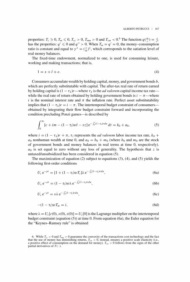
properties: Tc � 0, Tm � 0, Tcc > 0, Tmm > 0 and Tcm < 0.6 The function q( mc ) = e

ch

has the properties: q ′ � 0 and q ′′ > 0. When Tm = q ′ = 0, the money–consumptionratio is constant and equal to γ ∗ = ( c

m )∗, which corresponds to the satiation level ofreal money balances.

The fixed-time endowment, normalized to one, is used for consuming leisure,working and making transactions; that is,

1 = x + l + e. (4)

Consumers accumulate wealth by holding capital, money, and government bonds b,which are perfectly substitutable with capital. The after-tax real rate of return earnedby holding capital is (1 − τ k)r—where τ k is the ad valorem capital income tax rate—while the real rate of return obtained by holding government bonds is i − π—wherei is the nominal interest rate and π the inflation rate. Perfect asset substitutabilityimplies that (1 − τ k)r = i − π . The intertemporal budget constraint of consumers—obtained by integrating their flow budget constraint forward and incorporating thecondition precluding Ponzi games—is described by∫ ∞

0[c + im − (1 − τl)wl − vz] e− ∫ t

0 (1−τk )rdu dt = k0 + a0, (5)

where i = (1 − τ k)r + π , τ l represents the ad valorem labor income tax rate, k0 +a0 nonhuman wealth at time 0, and a0 = b0 + m0 (where b0 and m0 are the stockof government bonds and money balances in real terms at time 0, respectively).a0 is set equal to zero without any loss of generality. The hypothesis that z isuntaxed/unsubsidized has been considered in equation (5).

The maximization of equation (2) subject to equations (3), (4), and (5) yields thefollowing first-order conditions

Uc e−ρt = [1 + (1 − τl )wTc]λ e− ∫ t0 (1−τk )rdu, (6a)

Ux e−ρt = (1 − τl)wλ e− ∫ t0 (1−τk )rdu, (6b)

Us e−ρt = vλ e− ∫ t0 (1−τk )rdu, (6c)

−(1 − τl )wTm = i, (6d)

where λ = Uc[c(0), x(0), s(0)] = Uc[0] is the Lagrange multiplier on the intertemporalbudget constraint (equation (5)) at time 0. From equation (6a), the Euler equation forthe “Keynes–Ramsey rule” is obtained

6. While Tcc > 0 and Tmm > 0 guarantee the convexity of the transactions cost technology and the factthat the use of money has diminishing returns, Tcm < 0, instead, ensures a positive scale elasticity (i.e.,a positive effect of consumption on the demand for money). Tcm < 0 follows from the signs of the otherpartial derivatives of T ( · ).


ρ − d

dtln

{Uc

[1 + (1 − τl)wTc]

}= (1 − τk)r. (6e)

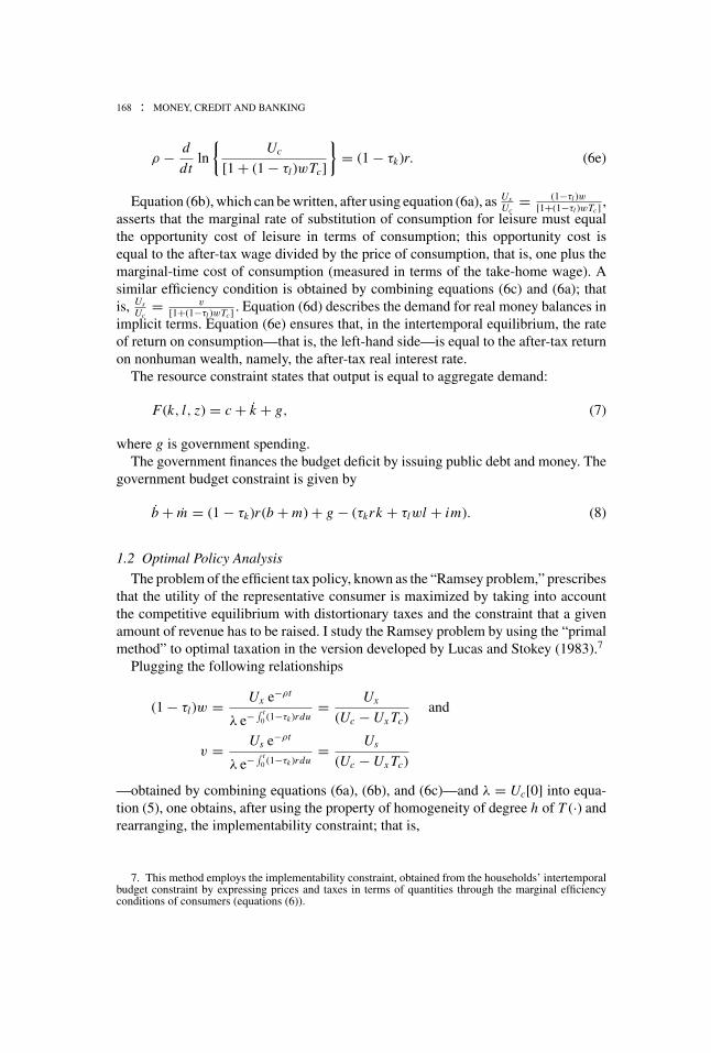
Equation (6b), which can be written, after using equation (6a), as UxUc

= (1−τl )w[1+(1−τl )wTc] ,

asserts that the marginal rate of substitution of consumption for leisure must equalthe opportunity cost of leisure in terms of consumption; this opportunity cost isequal to the after-tax wage divided by the price of consumption, that is, one plus themarginal-time cost of consumption (measured in terms of the take-home wage). Asimilar efficiency condition is obtained by combining equations (6c) and (6a); thatis, Us

Uc= v

[1+(1−τl )wTc] . Equation (6d) describes the demand for real money balances inimplicit terms. Equation (6e) ensures that, in the intertemporal equilibrium, the rateof return on consumption—that is, the left-hand side—is equal to the after-tax returnon nonhuman wealth, namely, the after-tax real interest rate.

The resource constraint states that output is equal to aggregate demand:

F(k, l, z) = c + k + g, (7)

where g is government spending.The government finances the budget deficit by issuing public debt and money. The

government budget constraint is given by

b + m = (1 − τk)r (b + m) + g − (τkrk + τlwl + im). (8)

1.2 Optimal Policy Analysis

The problem of the efficient tax policy, known as the “Ramsey problem,” prescribesthat the utility of the representative consumer is maximized by taking into accountthe competitive equilibrium with distortionary taxes and the constraint that a givenamount of revenue has to be raised. I study the Ramsey problem by using the “primalmethod” to optimal taxation in the version developed by Lucas and Stokey (1983).7

Plugging the following relationships

(1 − τl)w = Ux e−ρt

λ e− ∫ t0 (1−τk )rdu

= Ux

(Uc − Ux Tc)and

v = Us e−ρt


= Us

(Uc − Ux Tc)

—obtained by combining equations (6a), (6b), and (6c)—and λ = Uc[0] into equa-tion (5), one obtains, after using the property of homogeneity of degree h of T (·) andrearranging, the implementability constraint; that is,

7. This method employs the implementability constraint, obtained from the households’ intertemporalbudget constraint by expressing prices and taxes in terms of quantities through the marginal efficiencyconditions of consumers (equations (6)).


∫ ∞

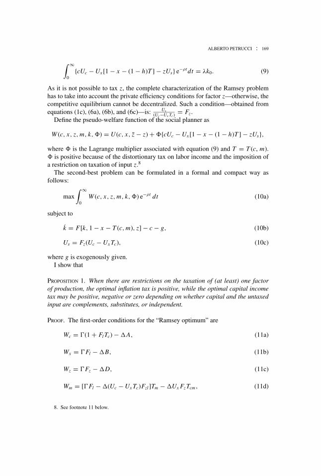
0{cUc − Ux [1 − x − (1 − h)T ] − zUs} e−ρt dt = λk0. (9)

As it is not possible to tax z, the complete characterization of the Ramsey problemhas to take into account the private efficiency conditions for factor z—otherwise, thecompetitive equilibrium cannot be decentralized. Such a condition—obtained fromequations (1c), (6a), (6b), and (6c)—is: Us

(Uc−Ux Tc) = Fz .Define the pseudo-welfare function of the social planner as

W (c, x, z, m, k,�) = U (c, x, z − z) + �{cUc − Ux [1 − x − (1 − h)T ] − zUs},

where � is the Lagrange multiplier associated with equation (9) and T = T (c, m).� is positive because of the distortionary tax on labor income and the imposition ofa restriction on taxation of input z.8

The second-best problem can be formulated in a formal and compact way asfollows:

max∫ ∞

0W (c, x, z, m, k,�) e−ρt dt (10a)

subject to

k = F[k, 1 − x − T (c, m), z] − c − g, (10b)

Us = Fz(Uc − Ux Tc), (10c)

where g is exogenously given.I show that

PROPOSITION 1. When there are restrictions on the taxation of (at least) one factorof production, the optimal inflation tax is positive, while the optimal capital incometax may be positive, negative or zero depending on whether capital and the untaxedinput are complements, substitutes, or independent.

PROOF. The first-order conditions for the “Ramsey optimum” are

Wc = �(1 + Fl Tc) − A, (11a)

Wx = �Fl − B, (11b)

Wz = �Fz − D, (11c)

Wm = [�Fl − (Uc − Ux Tc)Fzl]Tm − Ux FzTcm, (11d)

8. See footnote 11 below.


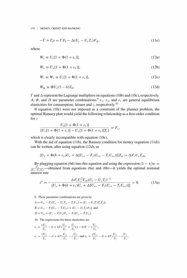
−� + �ρ = �Fk − (Uc − Ux Tc)Fzk, (11e)

where

Wc ≡ Uc[1 + �(1 + εc)], (12a)

Wx ≡ Ux [1 + �(1 + εx )], (12b)

Wz ≡ Ws ≡ Us[1 + �(1 + εs)], (12c)

Wm ≡ �Ux (1 − h)Tm . (12d)

� and represent the Lagrange multipliers on equations (10b) and (10c), respectively.A, B, and D are parameter combinations.9 εc, εx, and εs are general equilibriumelasticities for consumption, leisure and z, respectively.10

If equation (10c) were not imposed as a constraint of the planner problem, theoptimal Ramsey plan would yield the following relationship as a first-order conditionfor z

Us[1 + �(1 + εs)]

{Uc[1 + �(1 + εc)] − Ux [1 + �(1 + εx )]Tc} = Fz,

which is clearly incompatible with equation (10c).With the aid of equation (11b), the Ramsey condition for money (equation (11d))

can be written, after using equation (12d), as

{Ux + �(h + εx )Ux + [Usx − Fz(Ucx − TcUxx )]}Tm = FzUx Tcm .

By plugging equation (6d) into this equation and using the expression (1 − τl )w =Ux

(Uc−Ux Tc) —obtained from equations (6a) and (6b)—it yields the optimal nominalinterest rate

i∗ = − FzU 2x Tcm(Uc − Ux Tc)−1

{Ux + �(h + εx )Ux + [Usx − Fz(Ucx − TcUxx )]} > 0. (13a)

9. These parameter combinations are given by

A = Usc − Fz(Ucc − UxTcc − TcUxc) + (Uc − UxTc)Tc Fzl];

B = Usx − Fz(Ucx − TcUxx) + (Uc − UxTc)Fzl]; and

D = Uss + (Uc − TcUx)Fzz − Fz(Ucs − TcUxs).

10. The expressions for these elasticities are

εc = cUcc

Uc

− (l + hT )Uxc

Uc

+ Ux

Uc

(1 − h)Tc − zUsc

Uc

;

εx = cUcx

Ux− (l + hT )

Uxx

Ux− z

Usx

Ux; and εs = cUcs

Us− (l + hT )

Uxs

Us− z

Uss

Us.


As Tcm < 0, and and the denominator of equation (13a) are positive, the optimalmonetary policy is the Phelps (1973) rule, thus making it necessary to set a positiveinflation tax. This anti-Friedman result derives from the impossibility of taxing zoptimally, that is, > 0.

In the long run, by substituting the “modified golden rule,” derived from equa-tion (6e)—that is, ρ = (1 − τ k)Fk—into equation (11e), the optimal capital incometax rate is obtained; this is given by

τ ∗k =

�

(Uc − Ux Tc)Fzk

Fk≷ 0. (13b)

It is optimal to tax (subsidize) capital income if capital and the untaxed input areEdgeworth complementary (substitutable)—that is, Fzk > ( < ) 0. If k and z areindependent—that is, Fzk = 0—the Chamley–Judd result (i.e., τ ∗

k = 0) is obtained.The optimal labor tax rate—derived by contrasting the optimal conditions for the

private and Ramsey problems regarding c and x—is given by

τ ∗l = [UcUx�(εx − εc) + (Uc B − Ux A)]

(Uc − Ux Tc)(Wx + B). (13c)

τ ∗l is positive for plausible parameter values.11 �

When there are limitations on factor taxation, efficiency requires to raise revenuesby taxing money in addition to incomes from taxable inputs. Our results would remainvalid if z were taxed, but not at an optimal rate.

In a context in which the tax code is not sufficiently rich, the inflation tax representsan indirect way of taxing the untaxable inputs.12 If there were no restrictions on thetaxation of factor z, that is, = 0, the optimal taxes on money and capital incomewould both be zero.

The economic ratio of this optimal tax configuration is imputable to the invalidityof the Diamond and Mirrlees (1971) intermediate good result when there are lim-itations to the optimal tax setting, as has been demonstrated by Munk (1980). Themechanical motivation of our results, instead, is based on the fact that when additionalconstraints have to be imposed on the Ramsey problem, a second partial derivative

11. The optimal labor tax can be equivalently expressed as

τ ∗l = [(Uc − Ux Tc)(Wc + A) − Uc�]

Tc(Uc − Ux Tc)(Wx + B). (13c′)

From equation (13c), we get, after using equation (13c′), the following expression for �

� = (Uc − Ux Tc)(Wc + A) − Uc� + Tc(Ux A − Uc B)

UcUx Tc(εx − εc)> 0,

where εx > εc if a plausible utility function U (·) is considered.12. A similar result is found by Nicolini (1998) in a model with tax evasion.


of the transactions technology enters the first-order condition of the planner problemfor real money balances.

The simplest application of Proposition 1 is obtained when there are only twoinputs, labor and capital, and two tax instruments, that is, inflation and capital incometaxes. In this case, I get:

PROPOSITION 2. In an infinite-lived monetary model with elastic labor–leisure choices,Ramsey optimality prescribes positive taxation of money and capital if labor cannotbe taxed.

PROOF. The optimal condition for real money balances, obtained from equation (13a),implies a positive inflation tax. The Ramsey plan for the capital tax rate, once com-bined with the private efficiency condition (6e), yields equation (13b) with Flk thatnow replaces Fzk; thus, τ ∗

k > 0 as Flk > 0, because the production function is linearlyhomogeneous in k and l. �

2. MONOPOLISTIC COMPETITION AND TAXATION OF PROFITS

2.1 The Model

In this section, I turn my attention to the implications of product market power onthe optimality of the Friedman rule. For simplicity, I abandon the consideration of athird factor of production that cannot be taxed and focus on capital and labor alone.

Consider an infinitely lived monetary economy in which there are product mar-ket imperfections.13 The consideration of firms with market power is based on thesupply-side of the Benhabib and Farmer (1994) analysis. There are two sectors inthe economy: a final good sector, which is perfectly competitive, and an intermediategood sector, which is monopolistically competitive. The perfectly competitive sectorproduces a unique final good by using differentiated intermediate goods. The im-perfectly competitive sector, instead, produces intermediate goods by using physicalcapital and labor.

The final good y is produced by using the production function

y =(∫ 1

0y1−μ

i di

) 11−μ

, (14)

where yi represents the i th intermediate good, and i is continuous in the interval[0, 1]; μ ε [0, 1) is the reciprocal of the elasticity of substitution among intermediateinputs. Final good producing firms maximize profits by choosing the optimal quantityof each intermediate good. The first-order condition for profit maximization yieldsthe following input demand

13. The role of monopolistic competition for the validity of the Friedman rule has been investigatedby Schmitt-Grohe and Uribe (2004a), whose analysis is extended here to include endogenous capitalformation, as well as capital income and profit taxation.


pi

p=

(yi

y

)−μ

, (15)

where pi is the price of the i th intermediate good and p the price of the final good.Because the final sector is perfectly competitive, firms’ profits should be zero. This

requires that p = (∫ 1

0 pμ−1μ

i di)μ

μ−1 .

The technology used in the intermediate goods sector is given by

yi = F(ki , li ), (16)

where ki and li represent capital and labor used for producing intermediate good i th,respectively. F(·) satisfies the neoclassical properties of regularity and is constantreturns to scale.

If I use equation (15), the i th firm’s profit in the intermediate sector (measured interms of the final good) can be expressed as �i = yμy1−μ

i − wli − rki , where r isthe real rental on capital and w the real wage. The i th intermediate good producermaximizes �i by taking into account the production function (16). The first-orderconditions for his/her problem are

(1 − μ)yμy−μ

i Fki (ki , li ) = r, (17a)

(1 − μ)yμy−μ

i Fli (ki , li ) = w. (17b)

μ measures the degree of product market imperfections; if the market power of firmsis zero (i.e., μ = 0), the competitive case will be obtained.

I consider a situation of symmetric equilibrium in which ki = k, li = l, pi = p, andyi = y. In this situation, the real rental on capital and the real wage are given by

(1 − μ)Fk(k, l) = r, (17a′)

(1 − μ)Fl(k, l) = w. (17b′)

Profits in the intermediate good sector profits are positive and equal to � =μF(k, l).

The utility function of consumers, defined over the infinite time span, is∫ ∞

0U (c, x)e−ρt dt, (18)

where U (·) satisfies the usual properties of regularity.The transaction costs technology and the time allocation constraint are given by

equations (3) and (4), respectively. The consumers’ intertemporal budget constraintis


∫ ∞

0[c + im − (1 − τl )wl − (1 − ατk)�] e− ∫ t

0 (1−τk )rdu dt = k0, (19)

where α is a parameter taking values of either 0 or 1, and the value of governmentbonds and real money balances at t = 0 have been set equal to zero.

Dividends � enter equation (19) as consumers are the owners of firms. As profitsexert only income effects, their separate optimal taxation would prescribe a confisca-tory 100% rate. Because such an optimal taxation of profits is not feasible in practice,I consider two alternative regimes of profit taxation: one in which profits are untaxedand one in which they are taxed at the same rate as capital income. These two polarregimes can be captured through the dummy α. If α = 0, profits are tax free and onlythe capital income tax rate is chosen optimally; if, instead, α = 1, there is a commontax rate for capital income and profits, which is set optimally.14

Consumers maximize equation (18) subject to equations (3), (4), and (19). Thefirst-order conditions for the consumer problem are given by equations (6), with theexception of equation (6c), which now does not apply.

The feasibility constraint is given by equation (7), when y = F(k, l) is used.

2.2 Second-Best Problem and the Ramsey Plan

The Ramsey problem has to be devised in such a way as to realize the possibilitythat capital income and profits are taxed at the same rate.

By employing (1 − τl)w = Ux e−ρt


= Uxξ

—where ξ = (Uc − UxTc)—and λ =Uc[0], the implementability constraint can be expressed as∫ ∞

0{cUc − Ux [1 − x − (1 − h)T ] − (1 − ατk)�ξ} e−ρt dt = λk0. (20)

The efficient second-best tax structure is found by maximizing the utility functional(18) subject to the implementability constraint (20), the feasibility constraint (7) withF(k, l), and the Euler equation (6e), once the transaction technology (equation (3)), thetime allocation constraint (4), and the firms’ demand for capital (17a′) are taken intoaccount. The additional constraint (6e) is considered as τ k enters the implementabilityconstraint when profits are subject to taxation (i.e., α �= 0). Equation (6e) can bewritten as ξ = ξ [ρ − (1 − τk)r ] because, by using equations (6a) and (6b), it can beeasily shown that Uc

[1+(1−τl )wTc] = (Uc − Ux Tc) ≡ ξ .Now the Ramsey problem can be expressed as

max∫ ∞

0W (c, x, m, k, τk,�) e−ρt dt (21a)

subject to

k = F(k, 1 − x − T ) − c − g, (21b)

14. Note that the confiscatory taxation of profits can be obtained when α = 1τk

.


ξ = ξ [ρ − (1 − τk)(1 − μ)Fk], (21c)

ξ = (Uc − Ux Tc), (21d)

where

W (c, x, m, k, τk,�) = U (c, x) + �{cUc − Ux [1 − x − (1 − h)T ] − (1 − ατk)�ξ},

� > 0 is the Lagrange multiplier associated with equation (20), � = μF(k, l), andT = T (c, m).

My findings can be synthesized as follows

PROPOSITION 3. In a monopolistically competitive monetary model of capital forma-tion, in which the confiscatory taxation of profits is not practicable, the efficient taxstructure requires to tax labor and money, and to subsidize capital if profits cannotbe taxed. If capital income and profits are taxed equally, optimality calls for positivecapital and labor tax rates and a zero inflation tax.

PROOF. The first-order conditions for the Ramsey problem are

Wc = �(1 + Fl Tc) − �ξ (1 − τk)(1 − μ)Fkl Tc + (Ucc − Ux Tcc − TcUxc), (22a)

Wx = �Fl − �ξ (1 − τk)(1 − μ)Fkl + (Ucx − TcUxx ), (22b)

Wm = [�Fl − �ξ (1 − τk)(1 − μ)Fkl]Tm − Ux Tcm, (22c)

−� + �ρ = −�ξ (1 − ατk)�k + �Fk − �ξ (1 − τk)(1 − μ)Fkk, (22d)

−� + ρ� = −�(1 − ατk)� + �[ρ − (1 − τk)(1 − μ)Fk] + , (22e)

� = − α��

(1 − μ)Fk, (22f)

where

Wc ≡ Uc[1 + �(1 + ηc)] + �ξ (1 − ατk)�l Tc, (23a)

Wx ≡ Ux [1 + �(1 + ηx )] + �ξ (1 − ατk)�l, (23b)

Wm ≡ �[Ux (1 − h) + ξ (1 − ατk)�l]Tm, (23c)


with �j = μFj for j = k, l. �, �, and are Lagrange multipliers on equations (21b),(21c), and (21d), respectively; ηc and ηx represent general equilibrium elasticities forconsumption and leisure, respectively.15

In the steady state equilibrium, it can be easily obtained, by combining equa-tion (22e) and (22f), that = (1 − α)�μF . The optimal condition for real moneybalances (22c) can be expressed—after using equations (22b), (23), and the previousexpression for —as

{Ux [1 + �(ηx + h)] − (1 − α)��(Ucx − TcUxx )} Tm = (1 − α)��Ux Tcm .

By using equation (6c), the optimal nominal interest rate is

i∗ = − (1 − α)��U 2x Tcm(Uc − Ux Tc)−1

{Ux [1 + �(ηx + h)] − (1 − α)��(Ucx − TcUxx )} � 0. (24a)

Second-best optimality requires that i∗ > 0 if α = 0. Therefore, when profits aretaxed less than capital income (α < 1), the optimal monetary policy satisfies thePhelps (1973) rule. If, instead, capital income and profits are taxed at the same rate(i.e., α = 1), the Friedman rule is optimal.

The joint use of equations (17a′) and (6e) implies that, in the steady state,(1 − τ k)(1 − μ)Fk = ρ. Employing this equation together with equations (22d)and (22f) yields the following optimal capital income tax rate

τ ∗k = −

μ

[� − �ξ

(1 − α

F Fkk

F2k

)][�(1 − μ) + α�μξ

(1 − F Fkk

F2k

)] . (24b)

The sign of the optimal capital income tax is ambiguous. If α = 0, τ ∗k < 0 as � −

�ξ = ξ + �(Ucηc − UxηxTc) > 0. In this case, capital taxation alleviates thedistortionary role of market imperfections as suggested by Judd (2002). If insteadα = 1, τ ∗

k > 0 because the profit tax rate, constrained to be equal to the capital incometax rate, exerts only income effects.

The efficient labor income tax rate—derived by combining equations (6a), (6b),(22a), and (22b)—is given by

15. These elasticities are defined as

ηc = cUcc

Uc

− (l + hT )Uxc

Uc

+ Ux

Uc

(1 − h)Tc; and

ηx = cUcx

Ux− (l + hT )

Uxx

Ux.


τ ∗l =

(Wx − B)[(1 − μ)Uc + μUx Tc] + (1 − μ)

(Uc

Tc− Ux

)E − Ux (Wc − A)

[(1 − μ)(Uc − Ux Tc)(Wx − B + E/Tc)],

(24c)

where A, B and E are combinations of parameters.16 The existence of positive profits,that can be either taxed or untaxed, has no substantial implications for the optimallabor tax rate, which is plausibly positive. �

These results are to be ascribed to the good market imperfections, which imply thatpositive profits appear in the intertemporal budget constraint of consumers. Since �

and Tc are elements of the pseudo-welfare function of the social planner—by means ofthe implementability constraint (20)—Tcm < 0 enters directly the first-order conditionof the Ramsey problem for m, thus invalidating the Friedman “full liquidity” rule.

These findings generalize and extend the result of Schmitt-Grohe and Uribe (2004a)by showing that the zero inflation tax may be optimal also when profit taxation isnonconfiscatory. Here, what is new (in addition to the endogeneity of capital and theuse of capital taxation), and to some extent surprising, is that the Friedman rule isvalid if capital and profits are taxed at the same rate (α = 1). To be satisfied, the “fullliquidity rule” needs a flexible choice of the tax instrument on profits and capital.

Note that the violation of the Friedman rule is satisfied when α < 1 and � > 0 (i.e.,μ > 0) hold. In this case, the inflation tax constitutes an indirect way of taxing profits.The optimal taxation of profits at the same rate as capital income (i.e., α = 1) resultsin the validity of the zero inflation tax result; the same result is true when profits (i.e.,μ = 0) are absent.17 If instead μ = 0 and hence � = 0, the burden of taxation isborne by labor taxation alone because i∗ = 0 and τ ∗

k = 0. Moreover, the zero inflationtax result would be invalid if monopoly profits were taxed at a nonoptimal rate. Thisis because in such a case after-tax profits still enter the implementability constraint(20)—with a tax rate that is parametrically given—and their partial derivatives affectthe first-order conditions of the Ramsey problem (21).

Once again, the crucial factor for the invalidity of the Friedman rule is the existenceof restrictions on the set of fiscal instruments that can be optimally used. Now theDiamond and Mirrlees (1971) principle has become invalid because of positive profitsas shown by Stiglitz and Dasgupta (1971). With regard to the mechanics of the results,I can observe that the existence of monopolistic profits that are not optimally taxedor not taxed at the same rate as capital implies a change in the way in which thetransaction costs technology and its derivatives (i.e., the ultimate cause of the validityof the Friedman rule) enter the implementability constraint.

16. They are given by the expressions: A = (Ucc − Ux Tcc − TcUxc); B = (Ucx − TcUxx ); and E =�ξ (1 − τk )(1 − μ)Fkl Tc.

17. The Friedman rule would also be satisfied if monopoly profits were taxed at a confiscatory rate(i.e., α = 1

τk).


3. EXTENSIONS OF THE ANALYSIS

In this section, I discuss other cases of invalidity of the zero inflation tax result inperfectly competitive economies peopled by immortal agents facing homogeneoustransaction technologies. These new cases are obtained when there are either decreas-ing returns to scale in the reproducible inputs or exogenous government transfers.In particular, I analyze an economy with productive public goods, one with a fixedinput, and one with constant public transfers.

3.1 An Economy with Productive Public Goods

Consider a perfectly competitive monetary economy in which the governmentspends for a productive public good, g, that cannot be sold to firms. Productive publicspending, which is exogenosuly given, is financed through distortionary taxes onmoney and factor incomes. Suppose—as in Jones, Manuelli and Rossi (1993)—thatthe production function—that is, y = F(k, l, g)—is linearly homogeneous in capital,labor and g. The presence of the productive public good implies that there are positiveprofits, given by � = gFg.18

Profits enter the intertemporal budget constraint of consumers. Let us suppose thatprofits are either untaxed or taxed at the same rate as capital income. Therefore, theconsumer intertemporal budget constraint is still given by equation (19), when � =gFg.

The optimal tax structure is described by

PROPOSITION 4. In an immortal monetary model of capital accumulation with pro-ductive government spending—that cannot be sold to firms—and decreasing returnsto scale with respect to the reproducible inputs, second-best efficiency prescribestaxation of money and labor. Capital can be taxed or subsidized or left tax free de-pending on whether capital and productive public spending are complementary orsubstitutable or independent.

PROOF. See Petrucci (2008). �

3.2 An Economy with a Fixed Input

Consider a monetary economy with perfect competition and an exogenously giveninput, like, for example, land. The production function is given by the constant returnsto scale technology y = F(k, l, z). The firm demand for land is given by Fz(k, l,z) = v, where v is the real land reward. Land is inelastically supplied and fully usedin production. Therefore, its total amount can be normalized to one.

18. In the technological hypotheses considered here, the optimal capital tax rate differs from zero asshown by Jones, Manuelli, and Rossi (1993). If F(k, l, g) were homogeneous of degree one in k and lalone, profits as well as the optimal tax rate on capital income would be zero; see Judd (1999).


Land is at the same time a factor of production and an asset. If I denote the priceof land in real terms by q, qz will indicate the land value, that is, the amount ofnonhuman wealth devoted to land. Assuming that assets are perfectly substitutable,I have under perfect foresight: r = v

q + qq . If this condition is substituted in the

consumers’ flow budget constraint, an intertemporal budget constraint equivalent toequation (19) is obtained, after integrating forward and imposing the no Ponzi gamecondition. Profits are now replaced by land rents, that is, � = v(k, l) = Fz(k, l). Tworegimes for taxing pure rents are contemplated: tax exemption of rents and taxationof rents at the same rate as capital income.

I have that

PROPOSITION 5. In a monetary economy with an inelastically supplied input, settingthe tax on rent to zero implies the optimality of a positive inflation tax. If rents aretaxed at the same rate as capital income, the optimal inflation tax is zero. Capitaltaxation is governed by the Edgeworth complementarity/substitutability relationshipsbetween capital and the fixed factor.


3.3 An Economy with Exogenous Government Transfers

Consider a perfectly competitive economy with two inputs, labor and capital, andlump-sum transfers distributed by the government to consumers; these transfers—denoted by n once expressed in terms of the numeraire—are exogenously given.As these transfers are not fixed, once specified in terms of consumption, the relativeprices (and in particular the nominal interest rate) affect household disposable incomethrough a channel that has not been considered before. The intertemporal budgetconstraint of consumers in this two-factor economy is given by equation (5) if nreplaces vz, while the implementability constraint is given by equation (9) if (Uc −Ux Tc )n replaces zUs.

In this case, I have the following normative results.

PROPOSITION 6. When exogenous government transfers are considered in a standardmonetary model with a homogeneous transactions technology, the optimal taxes onmoney and labor are positive, while the optimal capital income tax is zero.


4. CONCLUDING REMARKS

Since the study of Phelps (1973) the question of the optimal inflation tax has beeninvestigated by applying Ramsey’s second-best analysis. Phelps (1973) demonstrates


the optimality of collecting revenues from seignorage, thus invalidating the Friedman(1969) zero inflation tax rule.

By applying the Ramsey approach to dynamic settings, some recent papers haveinstead obtained, although with some dissonance, the optimality of the Friedman rulein models with distortionary taxes. Among the dissonant contributions, Mulligan andSala-i-Martin (1997) emphasize that the validity of the Friedman rule is a matter offunctional forms for tastes and the shopping-time technology, while Schmitt-Groheand Uribe (2004a) argue that when there are product market imperfections, such arule is satisfied if and only if monopoly profits are taxed at a confiscatory rate.

In the optimal inflation tax literature developed so far, the consideration of anendogenous capital stock has been quite infrequent, while that of capital incometaxation is totally absent. In this article, on the contrary, I have adopted a broader per-spective by considering capital formation as well as capital and labor income taxationto explore the proposition that the optimal inflation tax is zero. I have discovered theexistence of a connection between the Friedman rule and the Chamley–Judd resulton the optimality of zero capital income tax as they have similar theoretical justifica-tions. In intertemporal optimizing models of capital formation with infinite horizonsand transactions technology, the Friedman rule is in general nonoptimal when thesecond-best capital tax rate is nonzero.

The paper has demonstrated the optimality of a positive inflation tax when thereare limitations on taxation of production factors or profits/rents. The nonoptimalityof the Friedman rule derives from the invalidity of the Diamond and Mirrlees (1971)principle.

The synopsis of the results of the paper is as follows:

(1) Perfect competition with restrictions on factor taxationWhen taxation of one factor of production is restricted, the optimal inflationtax is positive, while the optimal capital income tax may be positive, negativeor zero depending on whether capital and the untaxed input are complements,substitutes, or independent.

(2) Monopolistic competition with restrictions on profit taxationIn an economy with monopolistic firms, when profits cannot be taxed at aconfiscatory rate, the efficient tax structure requires the taxation of labor andmoney, and the subsidization of capital if profits cannot be taxed. If capitalincome and profits are taxed equally, optimality calls for positive capital andlabor tax rates and a zero inflation tax.

(3) Perfect competition and decreasing returns to scale with tax restrictions(i) An economy with productive public goods

In a model of capital accumulation with productive government spending anddecreasing returns to scale with respect to the reproducible inputs, second-best efficiency prescribes taxation of money and labor. Capital can be taxedor subsidized or left tax free depending on whether capital and productivepublic spending are complementary or substitutable or independent.

(ii) An economy with a fixed input


In a monetary economy with an inelastically supplied input, setting the taxon rent to zero implies the optimality of a positive inflation tax. If rentsare taxed at the same rate as capital income, the optimal inflation tax iszero. Capital taxation is governed by the complementarity/substitutabilityrelationships between capital and the fixed factor.

(4) Perfect competition with fixed government transfersWhen the government distributes exogenous transfers to consumers, the optimaltaxes on money and labor are positive, while the optimal capital income tax iszero.

To conclude, I have discovered, from a mechanical standpoint, that the optimality ofthe Friedman rule in models with shopping-time costs fails when: (i) partial derivativesof the transaction costs technology enter the implementability constraint and hencethe planner’s pseudo-welfare function and (ii) there are additional constraints facedby the social planner, which private agents do not face, involving partial derivativesof the transaction technology. These conditions are parallel to those established byJones, Manuelli and Rossi (1997, pp. 105–6) for the optimality of the zero capitalincome tax.

LITERATURE CITED

Abel, Andrew B. (1987) “Optimal Monetary Growth.” Journal of Monetary Economics, 19,37–50.

Atkinson, Anthony B., and Joseph E. Stiglitz. (1972) “The Structure of Indirect Taxation andEconomic Efficiency.” Journal of Public Economics, 1, 97–119.

Benhabib, Jess, and Roger E.A. Farmer. (1994) “Indeterminacy and Increasing Returns.”Journal of Economic Theory, 63, 19–41.

Bhattacharya, Joydeep, Joseph H. Haslag, and Antoine Martin. (2005) “Heterogeneity, Redis-tribution, and the Friedman Rule.” International Economic Review, 46, 437–54.

Chamley, Christophe. (1985) “On a Simple Rule for the Optimal Inflation Rate in Second BestTaxation.” Journal of Public Economics, 26, 35–50.

Chamley, Christophe. (1986) “Optimal Taxation of Capital Income in General Equilibriumwith Infinite Lives.” Econometrica, 54, 607–22.

Chari, Varadarajan V., Lawrence J. Christiano, and Patrick J. Kehoe. (1996) “Optimality of theFriedman Rule in Economies with Distorting Taxes.” Journal of Monetary Economics, 37,203–23.

Chari, Varadarajan V., and Patrick J. Kehoe. (1999) “Optimal Fiscal and Monetary Policy.” InHandbook of Macroeconomics, edited by John B. Taylor and Michael Woodford, Vol. 1C,pp. 1671–1745. Amsterdam: Elsevier Science.

Correia, Isabel H. (1996) “Should Capital Income Be Taxed in the Steady State?” Journal ofPublic Economics, 60, 147–51.

Correia, Isabel H., Juan-Pablo Nicolini, and Pedro Teles. (2008) “Optimal Fiscal and MonetaryPolicy: Equivalence Results.” Journal of Political Economy, 116, 141–70.


Correia, Isabel H., and Pedro Teles. (1996) “Is the Friedman Rule Optimal When Money Is anIntermediate Good?” Journal of Monetary Economics, 38, 223–44.

Correia, Isabel H., and Pedro Teles. (1999) “The Optimal Inflation Tax.” Review of EconomicDynamics, 2, 325–46.

De Fiore, Fiorella, and Pedro Teles. (2003) “The Optimal Mix of Taxes on Money, Consumptionand Income.” Journal of Monetary Economics, 50, 871–87.

Diamond, Peter A., and James A. Mirrlees. (1971) “Optimal Taxation and Public ProductionI: Production Efficiency” and “Optimal Taxation and Public Production II: Tax Rules.”American Economic Review, 61, 8–27, 261–78.

Faig, Miguel. (1988) “Characterization of the Optimal Tax on Money When It Functions as aMedium of Exchange.” Journal of Monetary Economics, 22, 137–48.

Friedman, Milton. (1969) “The Optimum Quantity of Money.” In The Optimum Quantity ofMoney and Other Essays, edited by Milton Friedman, pp. 1–50. Chicago: Aldine.

Guidotti, Pablo, and Carlos A. Vegh. (1993) “The Optimal Inflation Tax When Money ReducesTransactions Costs: A Reconsideration.” Journal of Monetary Economics, 31, 189–205.

Guo, Jang-Ting, and Kevin J. Lansing. (1999) “Optimal Taxation of Capital Income withImperfectly Competitive Product Markets.” Journal of Economic Dynamics and Control,23, 967–95.

Jones, Larry E., Rodolfo E. Manuelli, and Peter E. Rossi. (1993) “On the Optimal Taxation ofCapital Income.” NBER Working Paper No. 4525.

Jones, Larry E., Rodolfo E. Manuelli, and Peter E. Rossi. (1997) “On the Optimal Taxation ofCapital Income.” Journal of Economic Theory, 73, 93–117.

Judd, Kenneth L. (1985) “Redistributive Taxation in a Simple Perfect Foresight Model.”Journal of Public Economics, 28, 59–83.

Judd, Kenneth L. (1999) “Optimal Taxation and Spending in General Equilibrium CompetitiveGrowth Models.” Journal of Public Economics, 71, 1–26.

Kimbrough, Kent P. (1986) “The Optimum Quantity of Money Rule in the Theory of PublicFinance.” Journal of Monetary Economics, 18, 277–84.

Kocherlakota, Narayana R. (2005) “Optimal Monetary Policy: What We Know and What WeDon’t Know.” Federal Reserve Bank of Minneapolis Quarterly Review, 29, 10–19.

Lagos, Ricardo, and Randall Wright. (2005) “A Unified Framework for Monetary Theory andPolicy Analysis.” Journal of Political Economy, 113, 463–84.

Lucas, Robert E., and Nancy L. Stokey. (1983) “Optimal Fiscal and Monetary Policy in anEconomy without Capital.” Journal of Monetary Economics, 12, 55–93.

Mulligan, Casey B., and Xavier Sala i-Martin. (1997) “The Optimum Quantity of Money:Theory and Evidence.” Journal of Money, Credit, and Banking, 29, 687–715.

Munk, Knud J. (1980) “Optimal Taxation with Some Non-Taxable Commodities.” Review ofEconomic Studies, 47, 755–65.

Nicolini, Juan-Pablo. (1998) “Tax Evasion and the Optimal Inflation Tax.” Journal of Devel-opment Economics, 55, 215–32.

Petrucci, Alberto. (2008) “Nonoptimality of the Friedman Rule with Capital Income Taxation.”Nuffield College Working Paper, Oxford University.

Phelps, Edmund S. (1973) “Inflation in the Theory of Public Finance.” Swedish Journal ofEconomics, 75, 67–82.


Ramsey, Frank P. (1927) “A Contribution to the Theory of Taxation.” Economic Journal, 37,47–61.

Schmitt-Grohe, Stephanie, and Martin Uribe. (2004a) “Optimal Fiscal and Monetary Policyunder Imperfect Competition.” Journal of Macroeconomics, 26, 183–209.

Schmitt-Grohe, Stephanie, and Martin Uribe. (2004b) “Optimal Fiscal and Monetary Policyunder Sticky Prices.” Journal of Economic Theory, 114, 198–230.

Stiglitz, Joseph E., and Partha Dasgupta. (1971) “Differential Taxation, Public Goods andEconomic Efficiency.” Review of Economic Studies, 38, 151–74.

Woodford, Michael. (1990) “The Optimum Quantity of Money.” In Handbook of MonetaryEconomics, edited by Friedman Benjamin and Frank H. Hahn, Vol. 2, pp. 1067–1152.Amsterdam: North-Holland.

nonoptimality of the friedman rule with capital income taxation

Documents