non-hamiltonian modeling of squeezing and thermal disorder in driven oscillators
TRANSCRIPT
arX
iv:1
411.
7369
v2 [
quan
t-ph
] 8
Jan
201
5
Non-Hamiltonian modeling of squeezing and thermal disorder in driven oscillators
Sashwin Sewran,1, ∗ Konstantin G. Zloshchastiev,1, † and Alessandro Sergi1, 2, ‡
1 School of Chemistry and Physics, University of KwaZulu-Natal inPietermaritzburg, Private Bag X01, Scottsville 3209, South Africa
2KwaZulu-Natal Node, National Institute for Theoretical Physics (NITheP), South Africa(Dated: Received: 26 November 2014 [arXiv])
Recently, model systems with quadratic Hamiltonians and time-dependent interactions were stud-ied by Briegel and Popescu and by Galve et al in order to consider the possibility of both quantumrefrigeration in enzymes [Proc. R. Soc. 469 20110290 (2013)] and entanglement in the high tem-perature limit [Phys. Rev. Lett. 105 180501 (2010); Phys. Rev. A 81 062117 (2010)]. Followingthis line of research, we studied a model comprising two quantum harmonic oscillators driven by atime-dependent harmonic coupling. Such a system was embedded in a thermal bath represented intwo different ways. In one case, the bath was composed of a finite but great number of indepen-dent harmonic oscillators with an Ohmic spectral density. In the other case, the bath was moreefficiently defined in terms of a single oscillator coupled to a non-Hamiltonian thermostat. In bothcases, we simulated the effect of the thermal disorder on the generation of the squeezed states inthe two-oscillators relevant system. We found that, in our model, the thermal disorder of the bathdetermines the presence of a threshold temperature, for the generation of squeezed states, equal toT = 311.13 K. Such a threshold is estimated to be within temperatures where chemical reactionsand biological activity comfortably take place.
PACS numbers: 42.50.Dv, 05.30.-d, 07.05.Tp, 74.40.GhMathematics Subject Classification (2000): 82C10, 81S30, 00A72, 37N20Keywords: Quantum State Squeezing, Thermal Disorder, Quantum Dynamics, Wigner Function
1. INTRODUCTION
The idea that quantum mechanics plays a fundamentalrole in the functioning of living matter is both old and il-lustrious [1]. This concept has been recently revived bothby researchers in the field of quantum information the-ory [2] and by the steady accumulation of experimentalevidence supporting the relevance of high-temperaturequantum effects in organic molecules and biological sys-tems [3–6]. Moreover, it has been suggested that time-dependent couplings might lead to intra-molecular refrig-eration in enzymes [7] so that low temperatures, wherethe magnitude of quantum effects is greater, can bereached with a well-defined mechanism.
What is more relevant to the present work is that non-equilibrium conditions might enhance quantum dynam-ical effects in biological and condensed matter systems.For instance, quantum resonances have been found toraise the critical temperature of superfluid condensationby means of a mechanism similar to that provided bythe Feshbach resonance in ultra cold gases [8]. By anal-ogy, resonances have also been proposed to be relevant inhigh-temperature superconductors [9] and in living mat-ter [10]. Moreover, recent theoretical studies on modelsystems driven out of equilibrium [11–14] have supportedthe persistence of quantum entanglement [15, 16] at hightemperatures.
∗Electronic address: [email protected]†Electronic address: [email protected]‡Electronic address: [email protected]
The usual approach to the dynamics of open quan-tum systems is realized through master equations [17]or path integrals [18], for example. Non-harmonic andnon-Markovian dynamics prove to be a tough problemwhen attacked with these theoretical tools. In the presentwork, instead, we use the Wigner representation [19–21]of quantum mechanics and the generalization of tech-niques originally stemming frommolecular dynamics sim-ulations [22, 23]. In this work, such techniques are em-ployed to investigate the generation of squeezing [24, 25]at high temperature under non-equilibrium conditions.Our study is performed on a model of two harmonic os-cillators (representing two modes of an otherwise gen-eral condensed matter system) embedded in a dissipativebath. The oscillators are coupled in a time-dependentfashion in order to mimic the action of an external driving(which might also be caused by some unspecified confor-mational rearrangement of the bath) while the dissipativebath has been formulated in two alternative ways (whichprovide equivalent results in our simulations). In thefirst case, the bath is specified in terms of a finite num-ber of independent harmonic oscillators with an Ohmicspectral density. In the second case, the bath is real-ized through a single harmonic oscillator coupled to anon-Hamiltonian thermostat (i.e., a Nose-Hoover Chainthermostat [26]). Such a non-Hamiltonian thermostat isdefined in terms of two free parameters, mη1
and mη2,
which play the role of fictitious masses. We observedthat, for the model studied, the agreement between theresults (obtained by means of the two different represen-tations of the bath) is achieved within the range of values0.96 ≤ mη1
= mη2≤ 1.04.
It is known that when the environment is formed by
2
a single bath there can be decoherence-free degrees offreedom [27–29]. Hence, a single bath can be expectedto lead more easily to the preservation of quantum ef-fects in general. Nevertheless, there are circumstances inwhich a single bath is exactly what is required by thephysical situation. For example, when the relevant sys-tem is formed by a localized mode (in a somewhat smallmolecule) which is not under the influence of thermo-dynamic gradients, the modeling of the environment bymeans of a single bath appears to be physically sound. Inany case, it is worth mentioning that the computationalscheme presented in this work can be easily generalizedto describe multiple dissipative baths. Indeed, within apartial Wigner representation this has already been donein Ref. [30].Squeezed states have widespread applications, espe-
cially in experiments which are limited by quantumnoise[25]. The control of quantum fluctuations can beused to limit the sensitivity in quantum experiments.Some of these applications can be found in condensedmatter [31–33], in spectroscopy [34], in quantum informa-tion [35] and in gravitational wave detection [36]. Veryoften, squeezed states are the concern of quantum op-tics where the quadratic degrees of freedom are photons.However, in a condensed matter system, one still hasquadratic degrees of freedom, given by phonons, so thatthe theory of squeezing in quantum optics can be trans-lated to quantum condensed matter systems.If squeezing could be present at high temperatures
within biological macromolecules, one could speculateabout its role in the passage of a substrate through anion channel: the reduction (squeezing) of the amplitudeof the fluctuation of the substrate’s position might favorits passage through the channel. The squeezing of thefluctuations of only specific molecules (selectivity) mightarise from the resonance between the substrate’s molec-ular vibrations and the phonons characterizing the chan-nel (in analogy with what has been proposed in Ref. [37]concerning odor sensing). However, the above examplewill only be left as speculative motivation driving thepresent work, which is solely concerned with the mod-eling of thermal disorder in the squeezing of molecularvibrations. To this end, we adopt the Wigner represen-tation of quantum mechanics [19–21] and simulate nu-merically the quantum non-equilibrium statistics of ourmodel. For our quadratic Hamiltonian, quantum dynam-ics can be represented in terms of the classical evolu-tion of a swarm of trajectories with a quantum statistical
weight, which is determined by the chosen thermal initialconditions. Quantum averages are, therefore, calculatedin phase space, as in standard molecular dynamics sim-ulations [22, 23]. The generation of squeezed states ismonitored through the threshold values of the average ofsuitable dynamical properties [24, 25]. The dependenceof the generated amount of squeezing on the tempera-ture of the environment is investigated. It is found in ourmodel that there is a temperature threshold for squeezedstates generation. The temperature and the time scaleat which such a threshold is located are in the rangewhere the dynamics and chemical reactions in biologicalsystems occur.
The interest of the this work is twofold. Firstly, itis a methodological study aiming at verifying the effec-tiveness of simulation techniques (based on the Wignerrepresentation of quantum mechanics) when calculatingtime-dependent effects in open quantum systems. Atpresent, such techniques are not commonly used whenstudying open quantum systems. However, they promisea somewhat straightforward extension to non-harmoniccouplings and non-Markovian dynamics. Secondly, wefind that our model, under the conditions adopted for thecalculation in the present study, confirms that quantumsqueezing can be present at temperatures of relevance forbiological functioning.
This paper is structured in the following way. In Sec. 2we sketch the Wigner representation of quantum mechan-ics and its use in conjunction with temperature controlthrough a Nose-Hoover Chain non-Hamiltonian thermo-stat. In Sec. 3 we introduce our model, together with thedifferent ways we represent its dissipative environment.The algorithm for sampling the initial conditions, propa-gating the classical-like trajectories (which represent thequantum evolution of the Wigner function), and the waywe monitor the formation of squeezed states in the sim-ulation are illustrated in Sec. 4. Numerical results arediscussed in Sec. 5. Finally, our conclusions and perspec-tives are presented in Sec. 6.
2. WIGNER REPRESENTATION
The Wigner function, expressed in the position basis,is defined as a specific integral transform of the densitymatrix [19–21] ρ(t) of the system under study:
W (r, p, t) =1
(2π~)Nf
∫ +∞
−∞
dNf ye−ipy~
⟨
r +y
2
∣
∣
∣ρ(t)
∣
∣
∣r − y
2
⟩
, (1)
where Nf is the number of degrees of freedom and a mul-tidimensional notation is adopted, so that (r, p, y) stands
for (ri, pi, yi), with i = 1, ..., Nf . Using the Wigner rep-

3
resentation, quantum statistical averages are calculatedas
〈χ〉 =
∫ +∞
−∞
∫ +∞
−∞
W (r, p)χW (r, p)dNf rdNf p , (2)
where χW (r, p) is the Wigner representation of the quan-tum operator χ; such a representation is obtained by con-sidering an integral transform equal to those in Eq. (1)but without the pre-factor (2π~)−Nf . Since in generalthe Wigner function can have negative values because ofquantum interference [38], it is interpreted as a quasi-probability distribution function [19–21, 38, 39].
One of the advantages provided by the use of theWigner representation of quantum mechanics is that theequation of motion of the density matrix,
∂ρ
∂t= − i
~
[
H, ρ]
, (3)
is mapped onto the classical Liouville equation forW (q, p, t) when the Hamiltonian operator H of the sys-tem is quadratic. To see this, one can consider theHamiltonian operator of system comprising of N har-monic modes:
H =
N∑
n=1
(
1
2mP 2n +
1
2mω2
nR2n
)
. (4)
Here Pn, Rn and ωn are the momentum operator, posi-tion operator and frequency of mode n respectively. Forsimplicity, each mode is given equal mass m.The Wigner representation of the equation of motion (3)is, in general,
∂W (q, p, t)
∂t=
2
~HW sin
[
~
2
(←−∂
∂r
−→∂
∂p−←−∂
∂p
−→∂
∂r
)]
W (q, p, t).
(5)The Wigner-transformed Hamiltonian HW is obtainedfrom the quantum operator in Eq. (4) with the substi-
tution Pn → pn, Rn → rn, for n = 1, ..., N . However,since the Hamiltonian only contains quadratic terms inboth position and momentum, the Wigner equation ofmotion (5) reduces to the classical Liouville equation
∂W (q, p, t)
∂t=
(
∂HW
∂r
−→∂
∂p− ∂HW
∂p
−→∂
∂r
)
W (q, p, t). (6)
Equation (6) has a purely classical appearance whereasall quantum effects arise from the initial conditions.When the initial state of the N -oscillator system ispositive-definite (as in the case of a thermal state),Eq. (6) makes it possible to simulate the quantum dy-namics of a purely harmonic system via classical meth-ods.
In Ref. [40] it was shown how the quantum evolutionin the Wigner representation can be generalized in order
to control the thermal fluctuations of the phase spacecoordinates (r, p). This was achieved upon introducinga generalization of the Moyal bracket [41] that extendedthe Nose-Hoover thermostat [42, 43] to quantum Wignerphase space. Similarly, it was shown in [40] how to applythe so-called Nose-Hoover Chain (NHC) thermostat [26]to Wigner dynamics in order to achieve a proper tem-perature control for stiff oscillators. In the following, wewill briefly sketch the theory by specializing it to har-monic systems. However, since the Wigner NHC methodis not common in the theory of open quantum systems,we provide a somewhat extended introduction in Ap-pendix A. In order to introduce the Wigner NHC dynam-ics for harmonic systems, one can consider the Wigner-transformed Hamiltonian HW , introduce four additionalfictitious variables and define an extended Hamiltonianas
HNHC = HW +p2η1
2mη1
+p2η2
2mη2
+ gkBTextη1 + kBTextη2,
(7)where (η1, η2, pη1
, pη2) denote the fictitious variables with
masses mη1and mη2
, respectively. The symbol g denotesthe number of degrees of freedom to which the NHCthermostat is attached, kB is the Boltzmann constantand Text is the absolute temperature of the bath. Thephase space point of the extended system is defined asx = (r, η1, η2, p, pη1
, pη2) . Introducing the antisymmet-
ric matrix BNHC,
BNHC =
0 0 0 1 0 00 0 0 0 1 00 0 0 0 0 1−1 0 0 0 −p 00 −1 0 p 0 −pη1
0 0 −1 0 pη10
, (8)
it is possible to express the NHC equations of motionas [44–46]
xj = BNHCjk
∂HNHC
∂xk
, (9)
where the Einstein notation of summing over repeatedindices has been used. Hence, as shown in [40], in orderto achieve temperature control, Eq. (6) must be replacedby
∂W (x, t)
∂t= −∂W (x, t)
∂xj
BNHCjk
∂HNHC
∂xk
(10)
in the extended phase space. Equation (10) is calledthe Wigner NHC equation of motion. It also containsquantum-corrections over the fictitious NHC variables(η1, η2, pη1
, pη2). However, its was shown in Ref. [40] that
a classical limit on the dynamics of such variables can betaken in order to avoid spurious quantum effects and rep-resent only the thermal fluctuation of the environment.Further details can be found in Appendix A.
4
3. MODEL SYSTEM
In this work, we simulated a model comprising a rel-evant system and an environment. The relevant systemis given by two coupled quantum harmonic oscillators.The environment was represented in two different ways,which will be described in Secs. 3.1 and 3.2. Here, wefirst introduce the relevant system.
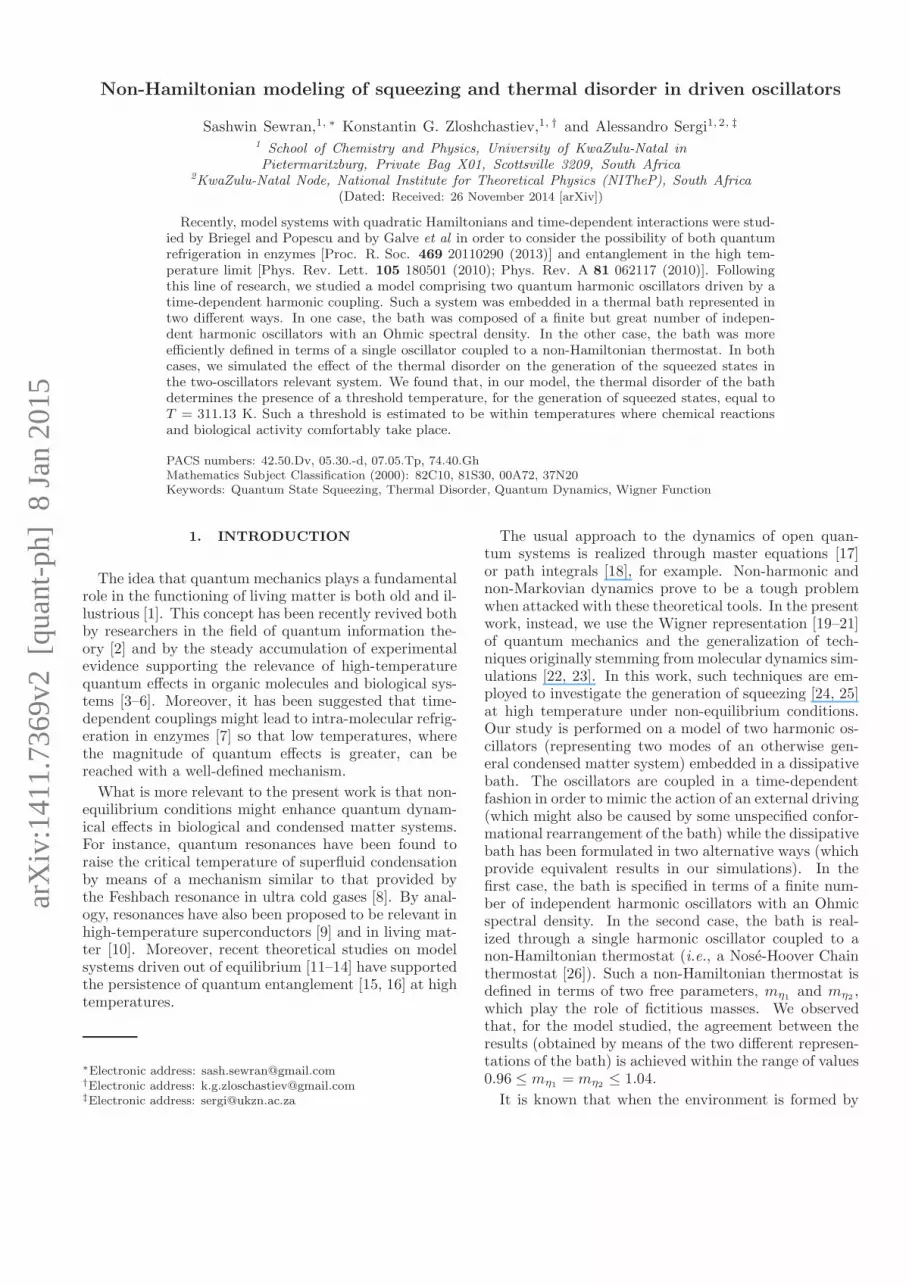
FIG. 1: Instability region (shaded area) in the parametricspace of the model (11), namely, in terms of values of (ω/ωd)
2
(horizontal axis) versus (ω0/ωd)2. The values reported on the
axes are in dimensionless units.
In the relevant system the coupling between the oscilla-tors is oscillatory, time-dependent and quadratic. In theWigner representation, the Hamiltonian of the system is
HS =p212m
+p222m
+mω2
2
(
q21 + q22)
+mω2(t)
2(q2 − q1)
2,
(11)where ω is the proper frequency of the oscillators, ω =√
K/m, and ω(t) is the time-dependent frequency of thecoupling between the oscillators
ω(t) ≡√
K(t)/m = ω0 sin (ωdt) . (12)
Here p1 and p2 are the momenta of the oscillators, m isthe mass of both oscillators, q1 and q2 are the displace-ment of the oscillators from their equilibrium positions,K is the spring constant of both oscillators, ω0 is theamplitude frequency of the coupling, ωd is the drivingfrequency and K(t) is the coupling function between theoscillators.
In Refs. [11] and [47] analytical solutions to similarmodels have been found. However, our system differs inthe time dependence of the coupling between the oscil-
lators. On a classical level our model can be treated interms of the Mathieu functions and using the Floquettheorem [48]. Using the notation defined in Appendix B(and assuming ωc ≡ ωd, where ωc is the frequency char-acterizing the spectral density of the bath introduced inSec. 3.1), we obtain the following equations of motion
d2Q′1
dt′2+
ω2
ω2d
Q′1 = 0 , (13)
d2Q′2
dt′2+
[
ω2 + ω20
ω2d
− ω20
ω2d
cos (2t′)
]
Q′2 = 0 , (14)
where Q′1 = (q′1 + q′2)/
√2 and Q′
2 = (q′1− q′2)/√2 are the
dimensionless center-of-mass and relative displacementcoordinates, respectively. While the solution of Eq. (13)is simply a linear combination of sine and cosine func-tions, Eq. (14) is the Mathieu equation and possessesmore complex features. In particular, for certain valuesof its parameters, it develops dynamical instabilities, seeFig. 1. Such parameters values must be avoided whendoing the numerical simulations in the quantum case.
3.1. Ohmic bath
In order to represent dissipative effects, the relevantsystem described by the HamiltonianHS was coupled, viaa bilinear coupling, to a bath of N independent harmonicoscillators with an Ohmic spectral density [49]. The totalHamiltonian is
HNB = HS +HB +HSB (15)
where
HB =
N∑
j=1
(
P 2j
2mj
+1
2mjΩ
2jR
2j
)
, (16)
HSB = −2∑
α=1
N∑
j=1
qαcjRj . (17)
The parameters in Eqs. (16) and (17) are defined as
Ωj = −ωc ln
(
1− jω0
ωc
)
(18)
ω0 =ωc
N
[
1− exp
(
−ωmax
ωc
)]
(19)
cj =√
ξ~ω0mjΩj . (20)
The frequency ωmax in Eq. (19) is a cut-off frequency usedin the numerical representation of the spectral density.The value of ωmax used in the calculations reported inthis work is given in Sec. 4. Each oscillator in the bathhas a different frequency, Ωj . The definition of Ωj , ω0 andcj is chosen in such a way to represent an infinite bath ofoscillators with Ohmic spectral density [49] in terms of
5
discrete mode of oscillations [50–52]. The parameters ξand ωc characterize the spectral density of the bath. TheKondo parameter, ξ, is a measure of the strength of thecoupling between the relevant system and the bath.
0
0.5
1
1.5
2
2.5
3
0 50 100 150 200 250
Nor
mal
mod
e va
rianc
es
Time
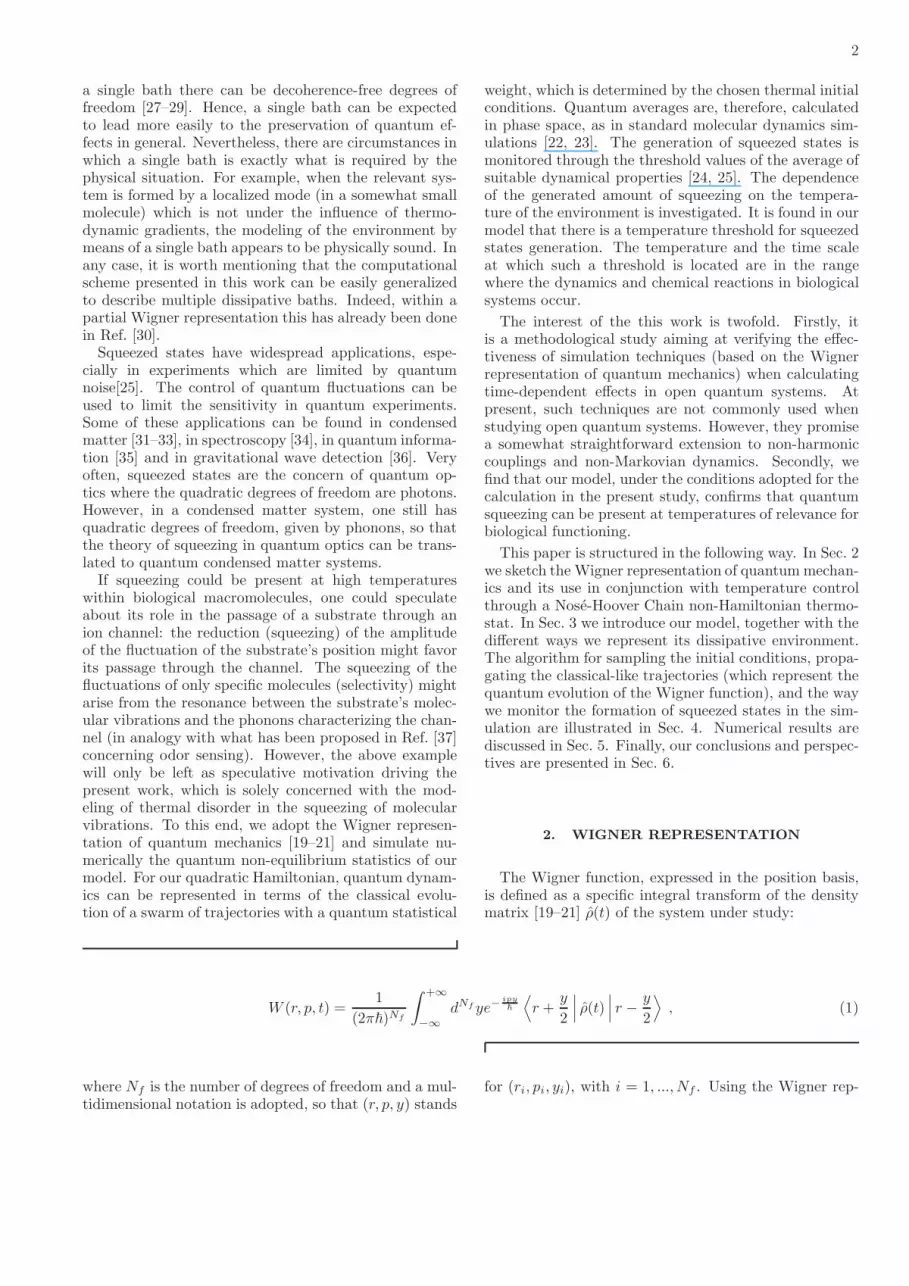
FIG. 2: Variance of the position and momentum coordinateof each normal mode, where the relevant system is attachedto a harmonic bath. The shaded square, circle, triangle anddiamond points represent the variances of R1, R2, P1 and P2
respectively. Solid lines, connecting the numerically calcu-lated points, have been drawn to guide the eye. Dimension-less parameters used in this simulation: m = 1.0, K = 1.25,ω0 = 2.50, ωd = 0.45, ξ = 0.007 and Text = 1.0. The valuesreported on the axes are also in dimensionless units.
3.2. NHC representation of the bath
We adopted a second technique to represent the dissi-pative environment in which the relevant driven systemis embedded. In particular, we considered a single os-cillator bilinearly coupled to the relevant system and wethermalized it by means of a Nose-Hoover Chain [26, 40].Such a technique (and similar ones [53, 54]) allows one toreduce drastically the computational time by represent-ing the thermal environment with a minimal number ofdegrees of freedom. In this case, the total Hamiltonian is
HNHC = HS +H1B +H1
SB +HTH , (21)
H1B =
P 21
2m1
+1
2MΩ2
1R21 , (22)
H1SB = −c1R1 (q1 + q2) , (23)
HTH =P 2η1
2mη1
+P 2η2
2mη2
+ kBTextη1 + kBTextη2 .(24)
Here P1 and R1 are the phase space variables of the bathoscillator having mass m1 and frequency Ω1. The bathand driven system are bilinearly coupled. The fictitiousNose variables are indicated by η1 and η2 while Pη1
andPη2
are their associate momenta. The fictitious Nose vari-
ables have massesmη1andmη2
, respectively. The symbolkB denotes the Boltzmann constant while Text indicatesthe absolute temperature of the bath. As explained withmore detail in Appendix A, the coupling to the fictitiousthermostat variables (η1, η2, pη1
, pη2) is realized through
the non-Hamiltonian equation of motion. In the classi-cal case, such equations are written in compact form inEq. (9) or in explicit form in Eqs. (A1-A6). In the quan-tum case, the coupling is given through Eq. (10). Thequantum-classical approximation of Eq. (10), which sup-presses the spurious quantum effects over the fictitiousNHC variables, is instead given in Eq. (A10). Equa-tion (A10) is the one used for the NHC representationof the bath in this work.
0.4
0.45
0.5
0.55
0.6
0.65
0.7
0.75
0.8
0.85
0.9
0 50 100 150 200 250
<(∆
R2)
2 >
Time
0.45
0.55
0.65
0.75
0.85
0 5 10 15 20
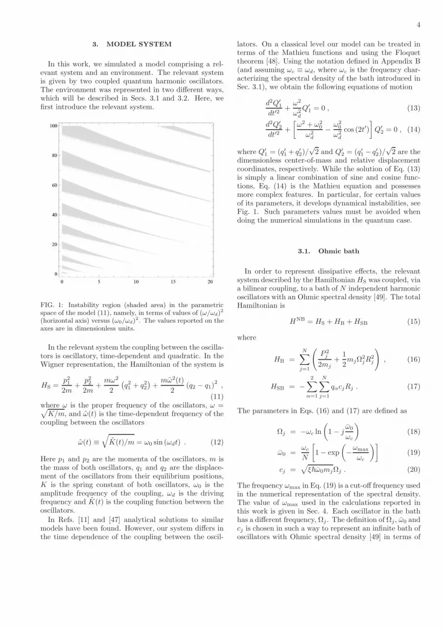
FIG. 3: Variance of the position coordinate of normal mode2, R2, where the relevant system is attached to a harmonicbath. A horizontal line at 〈(∆R2)
2〉=0.5 shows the theoreticalthreshold value for squeezed state generation. The inset showsthe short time simulation of the variance of R2, representedby solid circles. A solid line, connecting the numerically cal-culated points, has been drawn to guide the eye. Dimension-less parameters used in this simulation: m = 1.0, K = 1.25,ω0 = 2.50, ωd = 0.45, ξ = 0.007 and Text = 1.0. The valuesreported on the axes are also in dimensionless units.
4. SIMULATION DETAILS
The algorithm used to integrate the equations of mo-tion in all our simulations is based on the symmetricTrotter factorization of the propagator [55, 56]. When weconsidered the NHC thermostat to represent the thermalbath, we also incorporated the Yoshida scheme [57] withthree iterations and a multiple time-step procedure withthree iterations, following the approach of Ref. [55]. Inthe simulations, we set as initial conditions for the NHCvariables η1 = 0, η2 = 0, pη1
= 0 and pη2= 1.0.
At t = 0 it is assumed that the system is at thermalequilibrium with no time-dependent driving. The drivingacts for t > 0. In this case, the Wigner function of the

6
total system is positive definite and can be representedas a collection of points that are propagated accordingto Eq. (6), when the bath is represented by means of Noscillators with an Ohmic spectral density, or accordingto Eq. (10), when using the NHC bath.
In order to sample the initial configuration of the rel-evant system, it is useful to introduce normal coordi-nates [58]:
q1 =1√2(q1 + q2) , (25)
q2 =1√2(q1 − q2) , (26)
p1 =1√2(p1 + p2) , (27)
p2 =1√2(p1 − p2) , (28)
so that the Hamiltonian HS in Eq. (11) can be writtenas
HNM =2∑
k=1
(
p2k2m
+1
2mω2
kq2k
)
, (29)
where ωk (k = 1, 2) are the normal mode frequencies.The symbol q1 represents the motion of the centre of massof the system, while q2 represents the relative displace-ments of the oscillators. The normal mode frequencies ofeach mode are
ω1 =
√
K
m, (30)
ω2(t) =
√
K + 2K(t)
m. (31)
The initial conditions of the system are sampled from theWigner function [20]:
WS =
2∏
k=1
1
π~tanh
(
~ωk
2β
)
exp
(
− p2k2σ2
pk
)
exp
(
− q2k2σ2
qk
)
(32)where
σpk=
[
2
~mωk
tanh
(
~ωk
2β
)]− 1
2
, (33)
σqk =
[
2mωk
~tanh
(
~ωk
2β
)]− 1
2
. (34)
In the high temperature limit (T →∞, β → 0), theWigner distribution function in Eq. (32) reduces to theclassical canonical distribution function, Z−1 exp[−βHS].Hence, simply by changing the sampling of the initial con-ditions of the system, we can study the difference betweenthe classical and the quantum behavior of the system.
At t = 0, the Ohmic bath is also assumed to be at
thermal equilibrium with initial Wigner function equalto
WB =
N∏
k=1
1
π~tanh
(
~Ωk
2β
)
exp
(
− P 2k
2σ2Pk
)
exp
(
− R2k
2σ2Rk
)
(35)where
σPk=
[
2
~mΩk
tanh
(
~Ωk
2β
)]− 1
2
(36)
σRk=
[
2mΩk
~tanh
(
~Ωk
2β
)]− 1
2
. (37)
So that the initial Wigner function for the total systemis W = WS ×WB.When using the NHC representation of the bath, WB
in Eq. (35) reduces to W 1B (which is obtained considering
N = 1) while the initial condition of the NHC fictitious
variables are taken as∏2
n=1 δ(pηn−p0ηn
)δ(ηn−η0n), where(η0n, p
0ηn), n = 1, 2, are some arbitrary fixed values. In
such a case, the total initial Wigner function is W =WS ×W 1
B ×∏2
n=1 δ(pηn− p0ηn
)δ(ηn − η0n).Considering two arbitrary quantum operators, a and
b, satisfying the commutation relation [a, b] = ic, it isknown that there is a squeezed state if [24]
⟨
(∆aW)2⟩
<1
2|〈cW〉| or
⟨
(∆bW)2⟩
<1
2|〈cW〉| , (38)
where aW, bW and cW are the Wigner representation of
a, b and c, respectively, and ∆aW = aW − 〈aW〉. In thecase the normal mode coordinates, Eqs. (25-28), their
commutation relations are[
ˆqj , ˆpk
]
= i~δjk, j, k = 1, 2.
In dimensionless coordinates, the conditions of squeezingcan be written as
⟨
(∆qk)2⟩
<1
2or
⟨
(∆pk)2⟩
<1
2. (39)
Equation (39) provides a threshold for state squeezing.Upon defining χk = q2k − 〈qk〉2 or χk = p2k − 〈pk〉2 fork = 1, 2, one can use Eq. (2) in order to assess statesqueezing. The squeezed states can be visualized uponconstructing the marginal distribution functions of eachnormal mode from the numerical evolution of the totalWigner function.
5. NUMERICAL RESULTS
In all simulations we considered an integration timestep dt = 0.01, a number of molecular dynamics stepsNS = 25000, and a number of Monte Carlo steps NMC =10000. Unless stated otherwise, the results are reportedin dimensionless coordinates and scaled units. We per-formed simulations considering three different cases. Thefirst concerns the study of the driven oscillators without

7
the coupling to an external bath. The second deals withthe driven oscillators bi-linearly coupled to an Ohmicbath. The third concerns the driven oscillators coupled toa dissipative bath constituted by a single harmonic oscil-lator thermalized though a Nose-Hoover Chain. We didnot find any appreciable numerical difference between theresults obtained with the Ohmic bath or with the singleharmonic oscillator thermalized though a NHC thermo-stat.
In order to check our calculation scheme, we ran aseries of simulations without taking into account dissi-pative effects. Instead, we focused on the dynamics ofthe two coupled oscillators with the Hamiltonian givenin Eq. (11). The stability of the numerical algorithmwas tested by calculating the average value of the energywhen considering ω = ω0 (which amounts to switching offthe time-dependent coupling) in Eq. (11). Such an aver-age value was found to be conserved in one part over tenthousand. Upon reintroducing the time-dependent fre-quency in Eq. (11), we also verified that a squeezed stateis generated. Starting from a thermal state, the varianceof the position and momentum of each normal mode co-ordinate was calculated. The variance of the position ofnormal mode 2 was found to be below the threshold forsqueezing while the variance of the momentum of normalmode 2 increases simultaneously (in agreement with theHeisenberg uncertainty principle). This indicated thata squeezed state for the position coordinate of normalmode 2 had been generated.
0.4
0.5
0.6
0.7
0.8
0.9
1
0 50 100 150 200 250
<(∆
R2)
2 >
Time
0.46
0.48
0.5
0.52
0.54
160 180 200 220 240
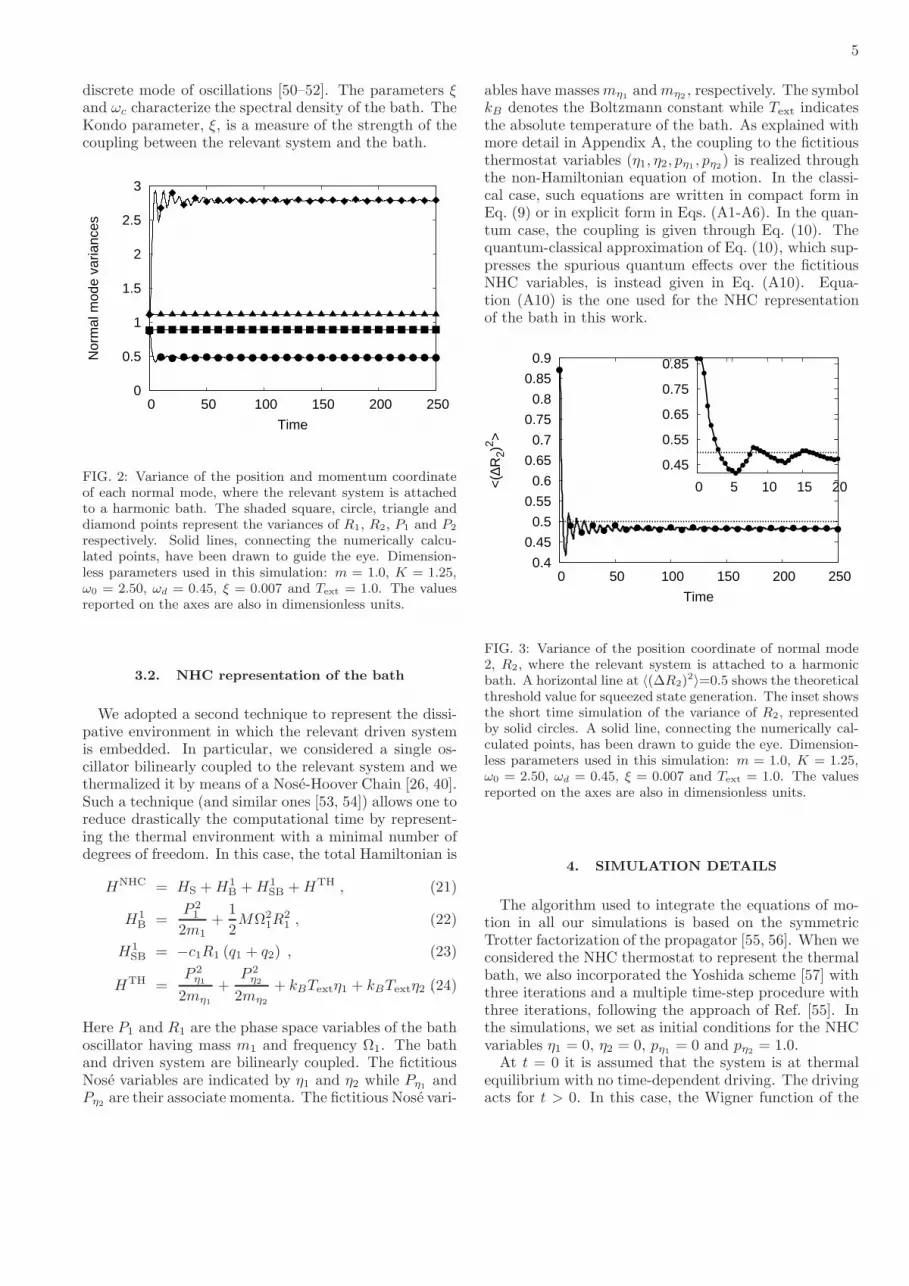
FIG. 4: Variance of normal mode coordinate R2, with threedifferent temperatures of the bath. The square, circle, andtriangle points are for temperatures of the bath 1.0, 1.037and 1.06, respectively. The inset shows the same curves inthe long-time region in order to better appreciate their differ-ences. Solid lines, connecting the numerically obtained points,have been drawn to guide the eye. Moreover, a horizontalline at 〈(∆R2)
2〉=0.5 shows the theoretical threshold value forsqueezed state generation. Dimensionless parameters used inthis simulation: m = 1.0, K = 1.25, ω0 = 2.50, ωd = 0.45,and ξ = 0.007. The values reported on the axes are also indimensionless units.
In order to account for dissipative effects and study theinfluence of a thermal bath on squeezed state generation,we used two methods that, as expected [53, 54], providednumerically indistinguishable results. In the first ap-proach, we used a bath of N = 200 harmonic oscillators,bi-linearly coupled to the system of driven oscillators. Ithas been shown that such a discrete representation ofthe Ohmic bath is in agreement with linear response the-ory [51, 52]. The Hamiltonian of this system is given inEq. (15). In the second approach, we represented thebath by means of a single oscillator coupled to a NHCthermostat. In this second case, the Hamiltonian of thesystem is given in Eq. (21). The values of the fictitiousmasses mη1
and mη2control the dynamics of the ther-
mostat, which in turn simulates the thermal bath. Suchmasses are tunable parameters that can be adjusted inorder to obtain an optimal agreement between the calcu-lations with N = 200 and no thermostat and those withN = 1 with the thermostat. In the calculations reportedin this work, we set mη1
= mη2= 1.0 (in dimensionless
units). We also observed that, for the model studied,the agreement between the results (obtained by means ofthe two different representations of the bath) is achievedwithin the range of values 0.96 ≤ mη1
= mη2≤ 1.04 of
the fictitious masses.
All calculations were performed using ωc = 1.0 andωmax = 3.0. Both weak and strong coupling strengths tothe bath (ξ = 0.007, 0.3) were studied. We observed thatthe coupling strengths influenced the behavior of normalmode 1 while normal mode 2 remained almost invari-ant. Figure 2 shows the variance of each normal modecoordinate. The variance of the coordinates of normalmode 1 maintain a constant value even when the driv-ing is switched on between the oscillators. However, weobserve a decrease in the variance of the position andan increase in the variance of the momentum of normalmode 2, respectively. This arises from the form of thenormal mode frequencies in Eqs. (30) and (31): only thefrequency of normal mode 2 is time-dependent, while thefrequency of normal mode 1 has a constant value. In Fig.3 we have plotted the theoretical threshold for squeezingas defined in Eq. (39). The variance of the position ofnormal mode 2 is clearly below such a threshold. Thisshows that the driven oscillators can make a transitionfrom a thermal to a squeezed state, as expected. Theinset in Fig. 3 shows the dynamics over a short time in-terval of the variance of the position of normal mode 2.The variance goes below the squeezing threshold after atime interval ∆t = 3.2 and remains below such a thresh-old for the rest of its time evolution. We can concludethat the generation of a squeezed state is fast in com-parison to the natural dynamics of the system. At timet = 0, the marginal distribution functions of both normalmodes are symmetrical and have a circular uncertaintydomain [59]. After the driving is turned on, the marginaldistribution function of normal mode 1 maintains its ini-tial features, while the marginal distribution function ofnormal mode 2 becomes asymmetrical with an elliptical

8
uncertainty domain.We also studied the influence of the temperature on
the degree of squeezing of the normal modes. In partic-ular, we have performed simulations for various valuesof the temperature ranging from 0.95 to 1.06 (and usedan increment of 0.01). In Figure 4, the results of threedifferent bath temperatures (Text=1.0, 1.037, and 1.06)are shown. The value of Text=1.037 provides a reliableestimate of the threshold temperature for the creation ofsqueezed states in our model, i.e., above this temperatureno squeezing is produced by the time-dependent dynam-ics. As a matter of fact, we verified that for Text=1.038we did not observe any squeezing. Below Text=1.037,for the various temperatures calculated, we have alwaysobserved the creation of squeezed states in our model.
6. CONCLUSIONS AND PERSPECTIVES
We studied the generation of squeezed states inducedby time-dependent quadratic coupling between two har-monic oscillators embedded in a dissipative environment.The latter was represented in two different ways thatprovided numerically indistinguishable results. In oneapproach, we used a bath of N = 200 harmonic oscil-lators with an Ohmic spectral density; in the other ap-proach, we used a single harmonic oscillator whose tem-perature was controlled through a Nose-Hoover Chainnon-Hamiltonian thermostat. The quantum equationsof motion were mapped onto a classical-like formalismthrough the Wigner representation and integrated nu-merically by means of standard molecular dynamics tech-niques. The systems studied are relevant in order tomodel the dynamics of molecular phonons (for example)in condensed matter.Upon varying the controlled temperature of the bath
in our calculations, we studied the effect of thermal dis-order on the generation of squeezing. It was found thatthere is a threshold temperature of the bath below whichsqueezing is still present. In dimensionless coordinates,this temperature is Text = 1.037. The non-Hamiltonianthermostat is defined in terms of two free parameters,mη1
and mη2, which play the role of fictitious masses.
We observed that, for the model studied, the agreementbetween the results (obtained by means of the two dif-ferent representations of the bath) is achieved within therange of values 0.96 ≤ mη1
= mη2≤ 1.04.
If we assume a value of the frequency ωc = 3.93× 10¹³
Hz we can convert to dimensionful coordinates and findthat such a temperature has the value Text = 311.13 K.According to this, the quantum of excitation ~ωc assumesthe value of 4.14 ×10⁻²¹ J, which is exactly equal to thevalue of kBT at room temperature (Text=300 K corre-sponding to Text = 1.0 in dimensionless coordinates).With the above value of ωc, we found two interestingresults. One is that the time spanned by the simulatedtrajectories is of the same order of magnitude as thatof molecular oscillations (≈ 1012 s). The second is that
the frequency of vibration of the relevant oscillators is ofthe order of the terahertz, as it is expected for molecularfunctional dynamics in biological systems [60]. Hence,our numerical study supports the possibility of havingobservable quantum effects at temperatures that are rel-evant for biological functions. As suggested by variousauthors [8, 11–14], such a counterintuitive occurrence ismade possible by the non-equilibrium conditions arisingin the dynamics of coupled molecular systems. In thiswork and elsewhere [8, 11–14], such complex situationshave been modeled through phononic modes with a time-dependent coupling. However, through a suitable modi-fication of the Wigner trajectory method, the techniquesillustrated in this paper promise a somewhat straight-forward extension to non-harmonic couplings and non-Markovian dynamics.
Acknowledgments
A. S. is grateful to Professor Salvatore Savasta forthe interesting discussions that motivated the presentwork. This research was supported through the IncentiveFunding for Rated Researchers by the National ResearchFoundation of South Africa. Besides, S. S. acknowledgesa Ph.D. bursary from the National Institute of Theoret-ical Physics (NITheP) in South Africa.
Appendix A: Wigner NHC equations of motion
Let us consider the Hamiltonian in Eq. (7) and theantisymmetric matrix in Eq. (8). The non-Hamiltonianequations on motion (9) are written explicitly as
r =p
m, (A1)
η1 =pη1
mη1
, (A2)
η2 =pη2
mη2
, (A3)
p = −∂V
∂r− pη1
mη1
p , (A4)
pη1=
p2
m− gkBT −
pη2
mη2
pη1, (A5)
pη2=
p2η1
m− kBT . (A6)
The Liouville operator for NHC dynamics is
LNHC = BNHCij
∂HNHC
∂xi
∂
∂xi
=p
m
∂
∂r+
pη1
mη1
∂
∂η1+
pη2
mη2
∂
∂η2
9
+
(
−∂V
∂r− pη1
mη1
p
)
∂
∂p
+
(
p2
m− gkBT
)
∂
∂pη
+
(
p2η1
m− kBT
)
∂
∂pη2
. (A7)
The above equations allow one to define NHC dynam-ics in classical phase space. The coupling between thethermostat momentum pη1
and the physical coordinatesp is not realized through the extended Hamiltonian inEq. (7). Instead, it is achieved through Eq. (A4). Under
the assumption of ergodicity, it can be proven that theNHC equations of motion (A1-A6) generate the canon-ical distribution function for the physical coordinates(r, p) [26, 44].
As originally explained in Ref. [40], the matrix formof the generalized Wigner bracket given in Eq. 10 canbe used to define NHC equations of motion in quantumphase space. Defining the phase space compressibility as
κ = (∂jBNHCji )∂iH
NHC , (A8)
the Wigner NHC equation can be written as
∂tW = −iLNHCW − κW +∑
n=3,5,7,...
1
n!
(
i~
2
)n−1
HNHC[←−∂iBNHC
ij
−→∂j +
←−∂i(∂jBN
ij)]n
fW , (A9)
where the Nose Liouville operator is defined as in Eq. (A7) andW = W (r, p, η1, η2, pη1, pη2
, t) is the Wigner distributionfunction in the extended NHC quantum phase space. To zeroth order in ~ the Nose-Wigner equations of motioncoincide with the classical equations of motion. Higher powers of ~ provide the quantum corrections to the dynamics.The quantum correction terms were considered in more detail in Ref. [40]. However, one is not really interested in thequantum behavior of the fictitious variables: they are there only to enforce the canonical distribution and representa thermal environment. Moreover, the mass mη1
is typically taken to be much greater than m in order to not modify
the dynamical properties of the system. As a result, one finds a small expansion parameter µ =√
m/mη1<< 1 that
can be used to take the classical limit over the (η1, η2, pη1, pη2
) fictitious variables. In such a way, in place of the fullquantum equation (A9) one obtains
∂tW = −(
iLNHC + κ)
W +∑
n=3,5,7,...
1
n!
(
i~
2
)n−1
V(←−∂ r
−→∂p
)n
W. (A10)
Equation (A10) defines a quantum-classical NHC dynamics according to which the (r, p) coordinates are evolvedquantum-mechanically while the (η1, η2, pη1
, pη2) are evolved classically. As proven in Ref. [40], the weak coupling
between the two sets of coordinates generates a canonical distribution function to zero order in ~.
Appendix B: Converting equations to dimensionless
form
It is convenient to introduce the following dimension-less variables:
q′i = qi
√
mωc
~, p′i =
pi√mEc
, (B1)
R′j = Rj
√
mjωc
~, P ′
j =Pj
√
mjEc
, (B2)
R′1 = R1
√
m1ωc
~, P ′
1 =P1√m1Ec
, (B3)
P ′η1
=Pη1
√
mη1Ec
, P ′η2
=Pη2
√
mη2Ec
, (B4)
t′ = ωct, H ′ =H
Ec
, T ′ =kBT
Ec
, (B5)
and
ω′(t′) =ω(t)
ωc
= ω′0 sin (ω
′dt
′) , (B6)
ω′ =ω
ωc
, ω′0 =
ω0
ωc
, ω′d =
ωd
ωc
, (B7)
ω′0 =
ω0
ωc
=1
N[1− exp (−ω′
max)] , (B8)
Ω′j =
Ωj
ωc
= − ln (1− jω′0) , (B9)
ω′max =
ωmax
ωc
, Ω′1 =
Ω1
ωc
, (B10)
and
c′j =cj
ωc
√
mmjΩjωc
=
√
ξ~ω′0Ω
′j
mωc
, (B11)

10
c′1 =c1
ωc
√mm1Ω1ωc
=
√
ξ~ω′0Ω
′1
mωc
, (B12)
where Ec = ~ωc and the indices i and j run from 1 to 2and from 1 to N , respectively. Also, the Hamiltonian Hand temperature T can carry any subscripts as prescribedby a model. Unless stated otherwise, all these definitionsare valid throughout the paper. Using them, the mainequations of the above-mentioned three models can bewritten as follows.The dimensionless Hamiltonian of the model in
Eq. (11) takes the form
H ′S =
p′212
+p′222
+ω′2
2
(
q′21 + q′22)
+ω′2(t)
2(q′2 − q′1)
2,
(B13)and the equations of motion for the dimensionless phase-space coordinates (q′1, q
′2, p
′1, p
′2) can be written as
dq′1dt′
= p′1, (B14)
dq′2dt′
= p′2, (B15)
dp′1dt′
= −ω′2q′1 + ω′2(t′) (q′2 − q′1) , (B16)
dp′2dt′
= −ω′2q′2 − ω′2(t′) (q′2 − q′1) . (B17)
As long as for this model the value ωc does not appear inthe Hamiltonian or elsewhere, for actual computationsone could naturally assume ωc ≡ κωd, where κ is anynatural number, for example.The dimensionless Hamiltonian of the model defined
in Eqs. (15-17) can be written as
H ′NB =
p′212
+p′222
+ω′2
2q′21 +
ω′2
2q′22
+ω′2(t)
2
(
q′22 − q′21)
+N∑
j=1
(
P ′2j
2+
1
2Ω′2
j R′2j
)
− (q′1 + q′2)
N∑
j=1
c′jR′j , (B18)
and the equations of motion for the dimensionless phase-space coordinates
(
q′1, q′2, R
′j , p
′1, p
′2, P
′j
)
are
dq′1dt′
= p′1, (B19)
dq′2dt′
= p′2, (B20)
dR′j
dt′= P ′
j , (B21)
dp′1dt′
= −ω′2q′1 + ω′2(t′) (q′2 − q′1) +
N∑
j=1
c′jR′j ,(B22)
dp′2dt′
= −ω′2q′2 − ω′2(t) (q′2 − q′1) +
N∑
j=1
c′jR′j ,(B23)
dP ′j
dt′= −Ω′2
j R′j + c′j (q
′1 + q′2) . (B24)
Finally, the dimensionless Hamiltonian of the NHCmodel (21) can be written as
H ′NHC =
p′212
+p′222
+ω′2
2q′21 +
ω′2
2q′22
+ω′2(t)
2(q′2 − q′1)
2+
P ′21
2+
ω′21
2R′2
1
− c′1R′1 (q
′1 + q′2) +
P ′2η1
2+
P ′2η2
2+ gT ′
extη1 + T ′extη2, (B25)
and the equations of motion for the dimensionless phase-space coordinates
(
q′1, q′2, R
′1, η1, η2, p
′1, p
′2, P
′1, P
′η1, P ′
η2
)
are
dq′1dt′
= p′1 , (B26)
dq′2dt′
= p′2 , (B27)
dR′1
dt′= P ′
1 , (B28)
dη1dt′
= P ′η1
, (B29)
dη2dt′
= P ′η2
, (B30)
dp′1dt′
= −ω′2q′1 + ω′2(t′) (q′2 − q′1) + c′1R′1 , (B31)
dp′2dt′
= −ω′2q′2 − ω′2(t) (q′2 − q′1) + c′1R′1 , (B32)
dP ′1
dt′= −Ω′2
j R′1 + c′1 (q
′1 + q′2) , (B33)
dP ′η1
dt′=(
P ′21 − gT ′
ext
)
− P ′η1P ′η2
, (B34)
dP ′η2
dt′= P ′2
η1− T ′
ext . (B35)

11
[1] E. Schrodinger, What is Life? Cambridge UniversityPress, Cambridge (2013).
[2] M. A. Chang and M. Nielsen, Quantum Computationand Quantum Information. Cambridge University Press,Cambridge (2011).
[3] G. S. Engel, et al., Nature 446, 782-786 (2007).[4] E. Collini, et al., Nature 463, 644-647 (2010).[5] G. Panitchayangkoon, et al., Proc. Natl Acad. Sci. 108,
20908-20912 (2011).[6] G. R. Fleming, S. F. Huelga, and M. B. Plenio, New J.
Phys. 13, 115002 pp. 5 (2011).[7] H. J. Briegel and S. Popescu, Proc. R. Soc. A 469,
20110290 pp. 9 (2013).[8] N. Poccia, A. Ricci, D. Innocenti, and A. Bianconi, Int.
J. Molec. Sci. 10, 2084-2106 (2009).[9] A. Valletta, et al., J. Superconductivity 10, 383-387
(1997).[10] A. W. Chin, A. Datta, F. Caruso, S. F. Huelga, and M.
B. Plenio, New J. Phys. 12, 065002 pp. 16 (2010).[11] F. Galve, L. A. Pachon and D. Zueco, Phys. Rev. Lett.
105, 180501 pp. 4 (2010).[12] F. Galve, G. L. Giorgi, and R. Zambrini, Phys. Rev. A
81, 062117 pp. 10 (2010).[13] G. G. Guerreschi, J. Cai, S. Popescu, H. J. Briegel, New
J. Phys. 14, 053043 pp. 21 (2012).[14] A. F. Estrada and L. A. Pachon, arXiv:1411.3382 [quant-
ph] (2014).[15] L. Amico, R. Fazio, A. Osterloh, and V. Vedral, Rev.
Mod. Phys. 80, 517-576 (2008).[16] R. Horodecki, P. Horodecki, M. Horodecki, and K.
Horodecki, Rev. Mod. Phys. 81, 865-942 (2009).[17] Irreversible Quantum Dynamics, Lecture Notes in
Physics, F. Benatti and R. Floreanini eds. (Springer,Berlin, 2013).
[18] U. Weiss, Quantum Dissipative Systems (World Scien-tific, Singapore, 2008).
[19] E. Wigner, Phys. Rev. 40, 749-759 (1932).[20] M. Hillery, R. F. O’Connell, M. O. Scully and E. P.
Wigner, Phys. Rep. 106, 121-167 (1984).[21] H. Lee, Phys. Rep. 259, 147-211 (1995).[22] M. P. Allen and D. J. Tildesley, Computer Simulation of
Liquids. Clarendon Press, Oxford (1989).[23] D. Frenkel and B. Smit, Understanding Molecular Simu-
lation. Academic Press, San Diego (2002).[24] C. C. Gerry and P. L. Knight, Introductory quantum
optics. Cambridge University Press, Cambridge (2005).[25] C. W. Gardiner and P. Zoller, Quantum Noise. Springer,
Berlin (2004).[26] G. J. Martyna, M. L. Klein and M. Tuckerman, J. Chem.
Phys. 97, 2635-2643 (1992).[27] P. Zanardi and M. Rasetti, Phys. Rev. Lett. 79, 3306
(1997).[28] D. A. Lidar, I. L. Chuang, and K. B. Whaley, Phys. Rev.
Lett. 81, 2594 (1998).[29] L.-M. Duan and G.-C. Guo, Phys. Rev. A 57, 737 (1998).
[30] A. Sergi, I. Sinayskiy, and F. Petruccione, Phys. Rev. A80, 012108 pp. 7 (2009).
[31] S. L. Johnson, et al., Phys. Rev. Lett. 102, 175503 pp. 4(2009).
[32] S.-L. Ma, P.-B. Li, A.-P. Fang, S.-Y. Gao, and F.-L. Li,Phys. Rev. A 88, 013837 pp. 5 (2013).
[33] T. Altanhan and B. S. Kandemir, J. Phys.: Condens.Matter 5, 6729-6736 (1993).
[34] D. J. Wineland, J. J. Bollinger, W. M. Itano, and D. J.Heinzen, Phys. Rev. A 50, 67-88 (1994).
[35] V. C. Usenko and R. Filip, New J. Phys. 13, 113007 pp.14 (2011).
[36] S. Dwyer, et al., Opt. Express 21, 19047-19060 (2013).[37] J. C. Brookes, F. Hartoutsiou, A. P. Horsfield, and A. M.
Stoneham, Phys. Rev. Lett. 98, 038101 (2007).[38] V. Zelevinsky, Quantum Physics; Vol. I. Wiley-VCH,
Weinhein (2011).[39] L. E. Ballentine, Quantum mechanics. World Scientific,
Amsterdam (2005).[40] A. Sergi and F. Petruccione, J. Phys. A 41, 355304 pp.
14 (2008).[41] J. E. Moyal, Proc. Camb. Philos. Soc. 45, 99-124 (1949).[42] S. Nose, Mol. Phys. 52, 255-268 (1984).[43] W. G. Hoover, Phys. Rev. A 31, 1695-1697 (1985).[44] A. Sergi and M. Ferrario, Phys. Rev. E. 64, 056125 pp.
9 (2001).[45] A. Sergi, Phys. Rev. E. 67, 021101 pp. 7 (2003).[46] A. Sergi and P. V. Giaquinta, J. Stat. Mech. 02, P02013
pp. 20 (2007).[47] E. A. Martinez and J. P. Paz, Phys. Rev. Lett. 110,
130406 pp. 4 (2013).[48] A. Lindner and H. Freese, J. Phys. A 27, 5565-5571
(1994).[49] A. J. Leggett, et al., Rev. Mod. Phys. 59, 1-85 (1987).[50] N. Makri and K. Thompson, J. Phys. Chem. 291, 101-
109 (1998).[51] K. Thompson and N. Makri, J. Chem. Phys., 110, 1343-
1353 (1999).[52] N. Makri, J. Phys. Chem. B, 103, 2823-2829 (1999).[53] N. Dlamini and A. Sergi, Comp. Phys. Comm. 184, 2474-
2477 (2013).[54] A. Sergi, J. Phys. A 40, F347-F354 (2007).[55] G. J. Martyna, M. E. Tuckerman, D. J. Tobias and M.
L. Klein, Mol. Phys. 87, 1117-1157 (1996).[56] A. Sergi, M. Ferrario and D. Costa, Molec. Phys. 97,
825-832 (1999).[57] H. Yoshida, Phys. Lett. A 150, 262-268 (1990).[58] H. Goldstein, Classical Mechanics. Addison-Wesley,
Reading MA (1980).[59] W. P. Schleich, Quantum Optics in Phase Space. Wiley,
Berlin (2001).[60] H. Zhang, K. Siegrist, D. F. Plusquellic and S. K. Gre-
gurick, J. Am. Chem. Soc. 130, 17846-17857 (2008).