Newtonian, Post Newtonian and Parameterized Post Newtonian limits of f(R,G)gravity

Mariafelicia De Laurentis1,2, Antonio Jesus Lopez-Revelles31,2Dipartimento di Fisica, Università di Napoli “Federico II”,

Compl. Univ. di Monte S. Angelo, Edificio G, Via Cinthia, I-80126, Napoli, Italy,INFN Sez. di Napoli, Compl. Univ. di Monte S. Angelo,

Edificio G, Via Cinthia, I-80126, Napoli, Italy and3 Consejo Superior de Investigaciones Científicas,

ICE/CSIC-IEEC, Campus UAB, Facultat de Ciencies,Torre C5-Parell-2a pl, E-08193 Bellaterra (Barcelona) Spain

(Dated: November 1, 2013)

We discuss in detail the weak field limit of f(R,G) gravity taking into account analytic functions ofthe Ricci scalar R and the Gauss-Bonnet invariant G. Specifically, we develop, in metric formalism,the Newtonian, Post Newtonian and Parameterized Post Newtonian limits starting from generalf(R,G) Lagrangian. The special cases of f(R) and f(G) gravities are considered. In the case of theNewtonian limit of f(R,G) gravity, a general solution in terms of Green’s functions is achieved.

Keywords: Alternative theories of gravity, weak field limit, theory of perturbations.

I. INTRODUCTION

Any good theory of physics should satisfy three main viability criteria that are self-consistency, completeness, andagreement with experiments. These have to hold also for theories of gravity like General Relativity (GR). However,despite its successes and elegance, such a theory exhibits a number of inconsistencies and weaknesses that have ledmany scientists to ask, whether, it is the final theory that can explain definitively the gravitational interaction. GRdisagrees with a growing number of data observed at infrared scales like cosmological scales. Furthermore, GR is notrenormalizable, because it presents singularities at ultraviolet scales (e.g. Big Bang singularity, black holes), and itfails to be quantized as standard quantum field theories.

Moreover, large amounts of dark matter and dark energy are required to address dynamics and structure of galaxies,clusters of galaxies and global accelerated expansion of the Hubble cosmic flow. If one wants to keep GR and its lowenergy limit, we must necessarily introduce these still unknown ingredients that, up to now, seem highly elusive. Inother words, GR, from ultraviolet to infrared scales, cannot be the ultimate theory of gravity even if it addresses awide range of phenomena.

In order to overcome the above mentioned problems and simultaneously obtain a semi-classical approach where GRand its results can be recovered, Extended Theories of Gravity (ETGs) have been recently introduced [1–6]. Thesetheories are based on corrections and extensions of Einstein’s theory. The effective Hilbert-Eintein action is modifiedby adding higher order terms in curvature invariants as R2, RµνRµν , RµνδρRµνδρ, R�R , R�nR or non-minimallycoupled terms between scalar fields and geometry as φ2R. The simplest generalization is the f(R) gravity where theHilbert-Einstein action, linear in the Ricci scalar R, is replaced by a generic function of it [7–11]. Such modificationsof GR generate inflationary behaviors which solve a lot of shortcomings of the Standard Cosmological Model as shownby Starobinsky [12], or can explain the flat rotation curves of galaxies or dynamics of galaxy clusters [13].

Another interesting curvature quantity that should be considered is the Gauss-Bonnet (GB) curvature invariantG defined below. This term can avoid ghost contributions and contribute to the regularization of the gravitationalaction [14–23]). Furthermore, in the case in which the Lagrangian density f is a function of G,i.e., f(G) it is possibleto construct viable cosmological models that are consistent with local constraints of GR [24–31].

In general, we can consider the most general Lovelock modification of gravity implying curvature and topologicalinvariant, that is L = f(R,G) [32]. Beyond the motivations for considering ETGs, it is important that we understandtheir weak-field limit from theoretical and experimental points of view. The Parameterized Post Newtonian (PPN)formalism is the first context for considering weak-field effects to test their viability with respect to GR. Eddington,Robertson and Schiff were the first that rigorously formulated the PPN formalism and used it in interpreting SolarSystems experiments [33–35]. After Nordvedt and Will fixed systematically the approach [36, 37].

Our aim, here, is to develop the weak field limit of f(R,G) considering the PPN formalism. Previous results havebeen developed for f(R) gravity in [38, 39] where the Post Newtonian (PN) limit is achieved by using the equivalencewith scalar-tensor theories [40]. On the other hand, the PN limit of Gauss-Bonnet gravity has been developed in [41]but not for pure f(G) gravity. Here, we develop the PPN limit for f(R,G), starting from the field equations. In doingso, we restrict our attention to those theories that admit a Minkowski background. Furthermore, as a special case,we develop the PPN limit even for the f(G) and then make a comparison with the results obtained for f(R).

2

The paper is organized as follows. In Sect. II, the field equations for f(R,G)-gravity theories are reviewed and theNewtonian, PN and PPN limits are obtained. In Sect. III, the Newtonian limit for f(R,G) gravities achieved in termsof Green’s functions. In Sect. IV, the weak field limit of the special cases of f(R) and f(G) modified gravities are,respectively, studied. Finally, in Sect. V, we summarize the obtained results and give some outlooks for the approach.

II. f(R,G) MODIFIED GRAVITY: THE FIELD EQUATIONS AND THE NEWTONIAN LIMIT

This section is devoted to the study of the field equations for f(R,G)-gravity and their Newtonian, PN and PPNlimits (for other examples of weak field limit in modified gravity theories, see [43–46]). The first remarkable character-istic of f(R,G) modified gravity is that, in this case, we obtain fourth–order field equations, instead of the standardsecond–order ones obtained in the case of GR. This fact is due to the existence of some boundary terms that disappearin GR thanks to the divergence theorem, but they remain in other theories, as in the case of f(R,G) gravity.

A. Field equations for f(R,G) gravity

The starting action for f(R,G) gravity is given by:

S =

∫d4x√−g{

1

2κ2f(R,G) + Lmatter

}, (1)

where Lmatter is the matter Lagrangian, g is the determinant of the metric, κ2 = 8πGN is standard gravitationalcoupling, and G is the Gauss-Bonnet invariant, defined as

G = R2 − 4RαβRαβ +RαβρσR

αβρσ. (2)

The variation of Eq.(1) with respect to the metric tensor gµν gives the field equations for f(R,G)-gravity that are:

−1

2gµνf(R,G) + fR(R,G)Rµν + gµν∇2 (fR(R,G))−∇µ∇ν (fR(R,G)) +

+2fG(R,G)RRµν − 4fG(R,G)RµρRρν + 2fG(R,G)RαβρµR

αβρν − 4fG(R,G)RµρνσR

ρσ+

+2gµνR∇2fG(R,G)− 4gµνRρσ∇ρ∇σfG(R,G)− 2R∇µ∇νfG(R,G)− 4Rµν∇2fG(R,G)+

+4Rνρ∇ρ∇µfG(R,G) + 4Rµρ∇ρ∇νfG(R,G) + 4Rµρνσ∇ρ∇σfG(R,G) = 2κ2Tµν . (3)

The trace equation is

−2f(R,G) + fR(R,G)R+ 3∇2fR(R,G) + 2fG(R,G)G + 2R∇2fG(R,G)− 4Rρσ∇ρ∇σfG(R,G) = 2κ2T. (4)

In Eq.(3) and Eq.(4), the following notation has been used: fR(R,G) =df(R,G)

dRand fG(R,G) = df(R,G)

dG , while ∇ isthe covariant derivative. The fact that the scalar curvature, R, and the Gauss-Bonnet invariant, G, involves secondderivatives of the metric tensor gµν makes of Eq.(3) and Eq.(4) fourth-order differential equations in the metric gµν .

B. The Newtonian, Post Newtonian and Parameterized Post Newtonian limits

All the quantities involved in the Newtonian, PN and PPN limits for f(R,G) gravity, given can be expanded inpowers of v̄2. As it is well known in the Solar System, the effects of the gravitational field are weak and are wellrepresented by Newton’s theory of gravity [42], therefore, the light rays travel on straight lines at a constant speedand the test particles move with an acceleration

a = ∇U ,

3

where U is the Newtonian potential produced by a rest mass density ρ according to following relations

∇2U = −4πρ , U(x, t) = GN

∫d3x′

ρ(x′, t)

|x− x′|.

The hydrodynamic equations for a perfect non-viscous fluid are the usual Eulerian equations

∂

∂t+∇ · (ρv) = 0 ,

ρdv

dt= ρ∇U −∇p ,

d

dt=

∂

∂t+ v · ∇ ,

where is the velocity of an element of the fluid, ρ is the density and p is the pressure on the element. This means

U ∼ p

ρ∼ v̄2 ∼ O(2) .

Also the derivatives with respect to the time relative to spatial derivatives are:

| ∂∂t || ∂∂x |

∼ O(1).

Here we have chosen to set c = 1. However, the Newtonian limit is no longer sufficient when we require that, inexperiments, accuracies go beyond 105 (e.g. it is not possible to explain, in the case of Mercury, the additionalperihelion advance greater than 5× 10−7 radians per orbit). Thus we need a more accurate approximation that goesbeyond the Newtonian approximation, and then the PN, PPN limits are considered. In order to build the PPN limitwe need of expanding in this order of smallness. To recover the Newtonian limit we must develop g00 up to O(2),while the PN limit requires

g00 up to O(4) ,

g0i up to O(3) ,

gij up to O(2) ,

where the Latin indices denote the spatial indices. These terms must contains factors as velocity or time derivatives.Furthermore these terms could represent energy dissipation or absorption. Beyond O(4), modified gravity effects cantake place and give different predictions. We expect that it should be possible to find a coordinate system where themetric tensor is nearly equal to the Minkowski tensor ηµν = diag(1,−1,−1,−1), the corrections being expandable inpowers of v̄2. We will consider the following ansatz for the metric tensor:

g00 = g(0)00 + g

(2)00 + g

(4)00 +O(6) with

{g(0)00 = 1

g(2)00 = −2U

g0i = g(3)0i +O(5)

gij = g(0)ij + g

(2)ij + g

(4)ij +O(6) with

{g(0)ij = −δijg(2)ij = −δij2V

(5)

where δij is the Kronecker delta and U, V are potentials, in particular V , following [42], is define as

Vi = GN

∫d3x′

ρ(x′, t)vi(x′, t)

|x− x′|. (6)

(7)

4

The inverse metric of Eq. (5) can be calculated using the relation gαρgρβ = δαβ , giving the following results:

g00 = g(0)00 + g(2)00 + g(4)00 +O(6) with

g(0)00 = 1g(2)00 = 2U

g(4)00 = −g(4)00 + 4U2

g0i = g(3)0i +O(5) with g(3)0i = δijg(3)0j

gij = g(0)ij + g(2)ij + g(4)ij +O(6) with

g(0)ij = −δijg(2)ij = δij2V

g(4)ij = −4V 2δij − δikδjlg(4)kl

(8)

Given a metric tensor, the associated connection associated can be derived as Γαµν = 12gαβ (∂µgνβ + ∂νgµβ − ∂βgµν) ,

which can be expanded in powers of v̄2 introducing, in the last equation, the expressions given by Eq. (5) and Eq.(8), namely:

Γ000 = Γ

(3)000 +O(5) with Γ

(3)000 = −∂0U

Γ00i = Γ

(2)00i + Γ

(4)00i +O(6) with

Γ(2)0

0i = −∂iU

Γ(4)0

0i = 12

(∂ig

(4)00 − 4U∂iU

)Γ0ij = Γ

(3)0ij +O(5) with Γ

(3)0ij = 1

2

(∂jg

(3)0i + ∂ig

(3)0j + 2δij∂0V

)

Γi00 = Γ(2)i

00 + Γ(4)i

00 +O(6) with

Γ(2)i

00 = −δil∂lU

Γ(4)i

00 = 12δil(∂lg

(4)00 + 4V ∂lU − 2∂0g

(3)0l

)Γi0j = Γ

(3)i0j +O(5) with Γ

(3)i0j = 1

2δil(∂lg

(3)0j − ∂jg

(3)0l + 2δlj∂0V

)

Γijk = Γ(2)i

jk + Γ(4)i

jk +O(6) with

Γ(2)i

jk = δil (−δjk∂lV + δlj∂kV + δlk∂jV )

Γ(4)i

jk = − 12δil[∂jg

(4)kl + ∂kg

(4)jl − ∂lg

(4)jk

]−

−2V δil [δlk∂jV + δlj∂kV − δjk∂lV ]

(9)

Given a metric tensor, the Riemann tensor, the Ricci tensor and the scalar curvature can be immediately calculatedby using the following expressions

Rαβρσ =1

2(∂σ∂αgβρ − ∂σ∂βgαρ − ∂ρ∂αgβσ + ∂ρ∂βgασ) + gµν

(ΓµσαΓνβρ − ΓµραΓνβσ

),

Rµν = ∂ρΓρµν − ∂µΓρρν + ΓρµνΓσρσ − ΓρσνΓσρµ,

R = gµνRµν . (10)

5

The components of the Riemann tensor that we will need later can be expanded in powers of v̄2 using Eqs. (5)-(10):

Ri0j0 = R(2)i0j0 +R

(4)i0j0 +O(6) with

R(2)i0j0 = ∂i∂jU

R(4)i0j0 = 1

2

(∂0∂ig

(3)0j + ∂0∂jg

(3)0i + 2δij∂0∂0V − ∂i∂jg(4)00

)+

+ (∂iU) (∂jU)− (∂iU) (∂jV )− (∂jU) (∂iV ) +

+δijδkl (∂kU) (∂lV )

R0ij0 = R(2)0ij0 +R

(4)0ij0 +O(6) with

R

(2)0ij0 = −R(2)

i0j0

R(4)0ij0 = −R(4)

i0j0

Rijk0 = R(3)ijk0 +O(5) with R

(3)ijk0 = 1

2

[∂k

(∂jg

(3)0i − ∂ig

(3)0j

)+ 2∂0 (δik∂jV − δjk∂iV )

]

(11)

By assuming the harmonic gauge, given by gµνΓρµν = 0 (in order to simplify the expressions), and using Eqs. (5)-(10),we can expand the Ricci tensor in powers of v̄2:

R00 = R(2)00 +R

(4)00 +O(6) with

R(2)00 = −4U

R(4)00 = 1

24g(4)00 + 2V4U + ∂0∂0U − 2δmn (∂mU) (∂nU)

R0i = R(3)0i +O(5) with R

(3)0i = 1

24g(3)0i

Rij = R(2)ij +R

(4)ij +O(6) with

R(2)ij = −δij4V

R(4)ij = 1

2

[∂0

(∂jg

(3)0i + ∂ig

(3)0j + 2δij∂0V

)−

−δmn(∂m

(∂ig

(4)nj + ∂jg

(4)ni

)− ∂i∂jg(4)mn

)+4g(4)ij − ∂i∂jg

(4)00

]+

+2V ∂i∂jV + 2U∂i∂jU + ∂iU ∂j(U − V )+

+∂iV ∂j(3V − U) + δij(δkl∂lV ∂k(U + V ) + 2V4V

)(12)

and the scalar curvature too:

R = R(2) +R(4) +O(6) with

R(2) = 34V −4U

R(4) = 124g

(4)00 + 2V (4U − 34V ) + ∂0∂0U − 2δij (∂iU) (∂jU)− 2U4U

(13)

On the matter side, we start with the general definition of the energy-momentum tensor of a perfect fluid:

Tµν = (ρ+ Πρ+ p)uµuν − pgµν , (14)

where Π denotes the internal energy density, ρ the energy density and p the pressure. Taking into account that:

u0 =1√

1− v2= 1 +

1

2v2 +

3

8v4 +O(6) ,

ui =vi√

1− v2= vi

(1 +

1

2v2 +O(4)

), (15)

6

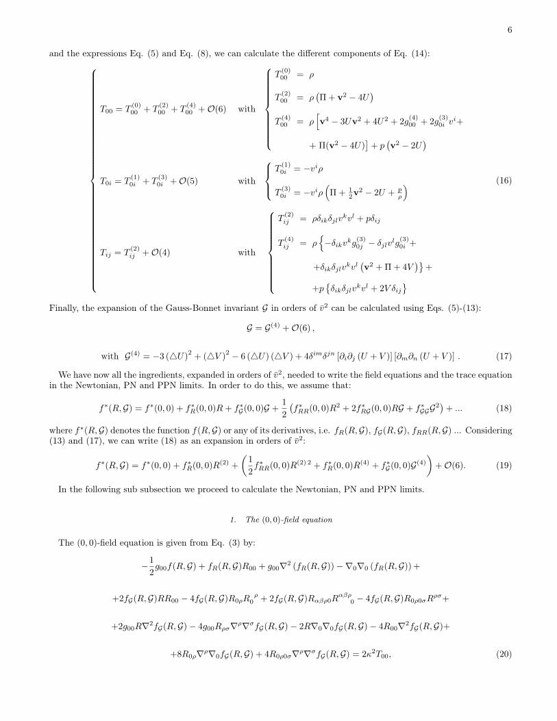
and the expressions Eq. (5) and Eq. (8), we can calculate the different components of Eq. (14):

T00 = T(0)00 + T

(2)00 + T

(4)00 +O(6) with

T(0)00 = ρ

T(2)00 = ρ

(Π + v2 − 4U

)T

(4)00 = ρ

[v4 − 3Uv2 + 4U2 + 2g

(4)00 + 2g

(3)0i v

i+

+ Π(v2 − 4U)]

+ p(v2 − 2U

)

T0i = T(1)0i + T

(3)0i +O(5) with

T

(1)0i = −viρ

T(3)0i = −viρ

(Π + 1

2v2 − 2U + p

ρ

)

Tij = T(2)ij +O(4) with

T(2)ij = ρδikδjlv

kvl + pδij

T(4)ij = ρ

{−δikvkg(3)0j − δjlvlg

(3)0i +

+δikδjlvkvl(v2 + Π + 4V

)}+

+p{δikδjlv

kvl + 2V δij}

(16)

Finally, the expansion of the Gauss-Bonnet invariant G in orders of v̄2 can be calculated using Eqs. (5)-(13):

G = G(4) +O(6) ,

with G(4) = −3 (4U)2

+ (4V )2 − 6 (4U) (4V ) + 4δimδjn [∂i∂j (U + V )] [∂m∂n (U + V )] . (17)

We have now all the ingredients, expanded in orders of v̄2, needed to write the field equations and the trace equationin the Newtonian, PN and PPN limits. In order to do this, we assume that:

f∗(R,G) = f∗(0, 0) + f∗R(0, 0)R+ f∗G(0, 0)G +1

2

(f∗RR(0, 0)R2 + 2f∗RG(0, 0)RG + f∗GGG2

)+ ... (18)

where f∗(R,G) denotes the function f(R,G) or any of its derivatives, i.e. fR(R,G), fG(R,G), fRR(R,G) ... Considering(13) and (17), we can write (18) as an expansion in orders of v̄2:

f∗(R,G) = f∗(0, 0) + f∗R(0, 0)R(2) +

(1

2f∗RR(0, 0)R(2) 2 + f∗R(0, 0)R(4) + f∗G(0, 0)G(4)

)+O(6). (19)

In the following sub subsection we proceed to calculate the Newtonian, PN and PPN limits.

1. The (0, 0)-field equation

The (0, 0)-field equation is given from Eq. (3) by:

−1

2g00f(R,G) + fR(R,G)R00 + g00∇2 (fR(R,G))−∇0∇0 (fR(R,G)) +

+2fG(R,G)RR00 − 4fG(R,G)R0ρRρ

0 + 2fG(R,G)Rαβρ0Rαβρ

0 − 4fG(R,G)R0ρ0σRρσ+

+2g00R∇2fG(R,G)− 4g00Rρσ∇ρ∇σfG(R,G)− 2R∇0∇0fG(R,G)− 4R00∇2fG(R,G)+

+8R0ρ∇ρ∇0fG(R,G) + 4R0ρ0σ∇ρ∇σfG(R,G) = 2κ2T00, (20)

7

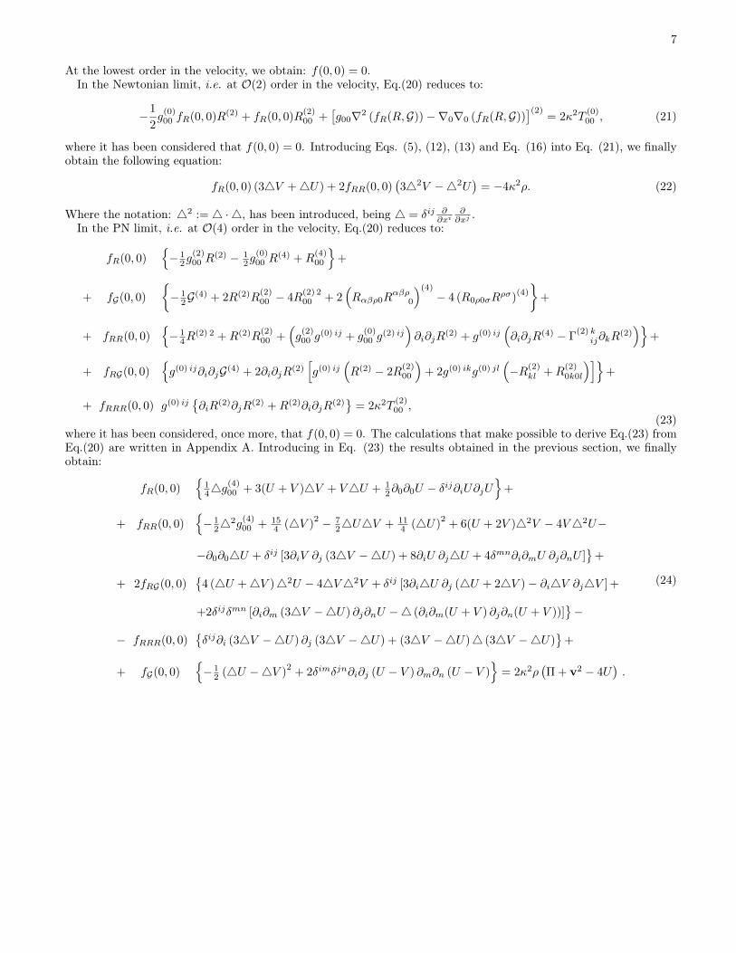
At the lowest order in the velocity, we obtain: f(0, 0) = 0.In the Newtonian limit, i.e. at O(2) order in the velocity, Eq.(20) reduces to:

−1

2g(0)00 fR(0, 0)R(2) + fR(0, 0)R

(2)00 +

[g00∇2 (fR(R,G))−∇0∇0 (fR(R,G))

](2)= 2κ2T

(0)00 , (21)

where it has been considered that f(0, 0) = 0. Introducing Eqs. (5), (12), (13) and Eq. (16) into Eq. (21), we finallyobtain the following equation:

fR(0, 0) (34V +4U) + 2fRR(0, 0)(342V −42U

)= −4κ2ρ. (22)

Where the notation: 42 := 4 · 4, has been introduced, being 4 = δij ∂∂xi

∂∂xj .

In the PN limit, i.e. at O(4) order in the velocity, Eq.(20) reduces to:

fR(0, 0){− 1

2g(2)00 R

(2) − 12g

(0)00 R

(4) +R(4)00

}+

+ fG(0, 0)

{− 1

2G(4) + 2R(2)R

(2)00 − 4R

(2) 200 + 2

(Rαβρ0R

αβρ0

)(4)− 4 (R0ρ0σR

ρσ)(4)

}+

+ fRR(0, 0){− 1

4R(2) 2 +R(2)R

(2)00 +

(g(2)00 g

(0) ij + g(0)00 g

(2) ij)∂i∂jR

(2) + g(0) ij(∂i∂jR

(4) − Γ(2) k

ij∂kR(2))}

+

+ fRG(0, 0){g(0) ij∂i∂jG(4) + 2∂i∂jR

(2)[g(0) ij

(R(2) − 2R

(2)00

)+ 2g(0) ikg(0) jl

(−R(2)

kl +R(2)0k0l

)]}+

+ fRRR(0, 0) g(0) ij{∂iR

(2)∂jR(2) +R(2)∂i∂jR

(2)}

= 2κ2T(2)00 ,

(23)where it has been considered, once more, that f(0, 0) = 0. The calculations that make possible to derive Eq.(23) fromEq.(20) are written in Appendix A. Introducing in Eq. (23) the results obtained in the previous section, we finallyobtain:

fR(0, 0){

144g

(4)00 + 3(U + V )4V + V4U + 1

2∂0∂0U − δij∂iU∂jU

}+

+ fRR(0, 0){− 1

242g

(4)00 + 15

4 (4V )2 − 7

24U4V + 114 (4U)

2+ 6(U + 2V )42V − 4V42U−

−∂0∂04U + δij [3∂iV ∂j (34V −4U) + 8∂iU ∂j4U + 4δmn∂i∂mU ∂j∂nU ]}

+

+ 2fRG(0, 0){

4 (4U +4V )42U − 44V42V + δij [3∂i4U ∂j (4U + 24V )− ∂i4V ∂j4V ] +

+2δijδmn [∂i∂m (34V −4U) ∂j∂nU −4 (∂i∂m(U + V ) ∂j∂n(U + V ))]}−

− fRRR(0, 0){δij∂i (34V −4U) ∂j (34V −4U) + (34V −4U)4 (34V −4U)

}+

+ fG(0, 0){− 1

2 (4U −4V )2

+ 2δimδjn∂i∂j (U − V ) ∂m∂n (U − V )}

= 2κ2ρ(Π + v2 − 4U

).

(24)

8

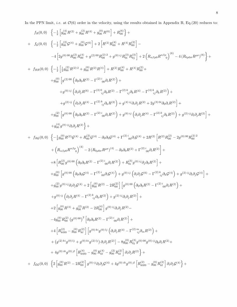
In the PPN limit, i.e. at O(6) order in the velocity, using the results obtained in Appendix B, Eq.(20) reduces to:

fR(0, 0){− 1

2

[g(4)00 R

(2) + g(2)00 R

(4) + g(0)00 R

(6)]

+R(6)00

}+

+ fG(0, 0){− 1

2

[g(2)00 G(4) + g

(0)00 G(6)

]+ 2

[R(2)R

(4)00 +R(4)R

(2)00

]−

−4[2g(0) 00R

(2)00 R

(4)00 + g(2) 00R

(2) 200 + g(0) ijR

(3)0i R

(3)0j

]+ 2

(Rαβρ0R

αβρ0

)(6)− 4 (R0ρ0σR

ρσ)(6)

}+

+ fRR(0, 0){− 1

2

[12g

(2)00 R

(2) 2 + g(0)00 R

(2)R(4)]

+R(2)R(4)00 +R(4)R

(2)00 +

+g(0)00

[g(2) 00

(∂0∂0R

(2) − Γ(2) i

00∂iR(2))

+

+g(0) ij(∂i∂jR

(6) − Γ(3) 0

ij∂0R(2) − Γ

(2) kij∂kR

(4) − Γ(4) k

ij∂kR(2))

+

+g(2) ij(∂i∂jR

(4) − Γ(2) k

ij∂kR(2))

+ g(4) ij∂i∂jR(2) + 2g(3) 0i∂0∂iR

(2)]

+

+g(2)00

[g(0) 00

(∂0∂0R

(2) − Γ(2) i

00∂iR(2))

+ g(0) ij(∂i∂jR

(4) − Γ(2) k

ij∂kR(2))

+ g(2) ij∂i∂jR(2)]

+

+g(4)00 g

(0) ij∂i∂jR(2)}

+

+ fRG(0, 0){− 1

2g(0)00 R

(2)G(4) +R(2)00 G(4) − ∂0∂0G(4) + Γ

(2) i00∂iG(4) + 2R(2)

[R(2)R

(2)00 − 2g(0) 00R

(2) 200

+(Rαβρ0R

αβρ0

)(4)− 2 (R0ρ0σR

ρσ)(4) − ∂0∂0R(2) + Γ

(2) i00∂iR

(2)

]+

+8[R

(2)00 g

(0) 00(∂0∂0R

(2) − Γ(2) i

00∂iR(2))

+R(3)0i g

(0) ij∂j∂0R(2)]

+

+g(0)00

[g(0) 00

(∂0∂0G(4) − Γ

(2) i00∂iG(4)

)+ g(0) ij

(∂i∂jG(6) − Γ

(2) kij∂kG(4)

)+ g(2) ij∂i∂jG(4)

]+

+g(2)00 g

(0) ij∂i∂jG(4) + 2[g(0)00 R

(2) − 2R(2)00

] [g(0) 00

(∂0∂0R

(2) − Γ(2) i

00∂iR(2))

+

+g(0) ij(∂i∂jR

(4) − Γ(2) k

ij∂kR(2))

+ g(2) ij∂i∂jR(2)]

+

+2[g(0)00 R

(4) + g(2)00 R

(2) − 2R(4)00

]g(0) ij∂i∂jR

(2)−

−4g(0)00 R

(2)00

(g(0) 00

)2 [∂0∂0R

(2) − Γ(2) i

00∂iR(2)]

+

+4[R

(2)k0l0 − g

(0)00 R

(2)kl

] [g(0) kig(0) lj

(∂i∂jR

(4) − Γ(2)m

ij∂mR(2))

+

+(g(2) kig(0) lj + g(0) kig(2) lj

)∂i∂jR

(2)]− 8g

(0)00 R

(3)0j g

(0) 00g(0) ij∂0∂iR(2)+

+ 4g(0) ikg(0) jl[R

(4)k0l0 − g

(0)00 R

(4)kl − g

(2)00 R

(2)kl

]∂i∂jR

(2)}

+

+ fGG(0, 0){

2[g(0)00 R

(2) − 2R(2)00

]g(0) ij∂i∂jG(4) + 4g(0) ikg(0) jl

[R

(2)k0l0 − g

(0)00 R

(2)kl

]∂i∂jG(4)

}+

9

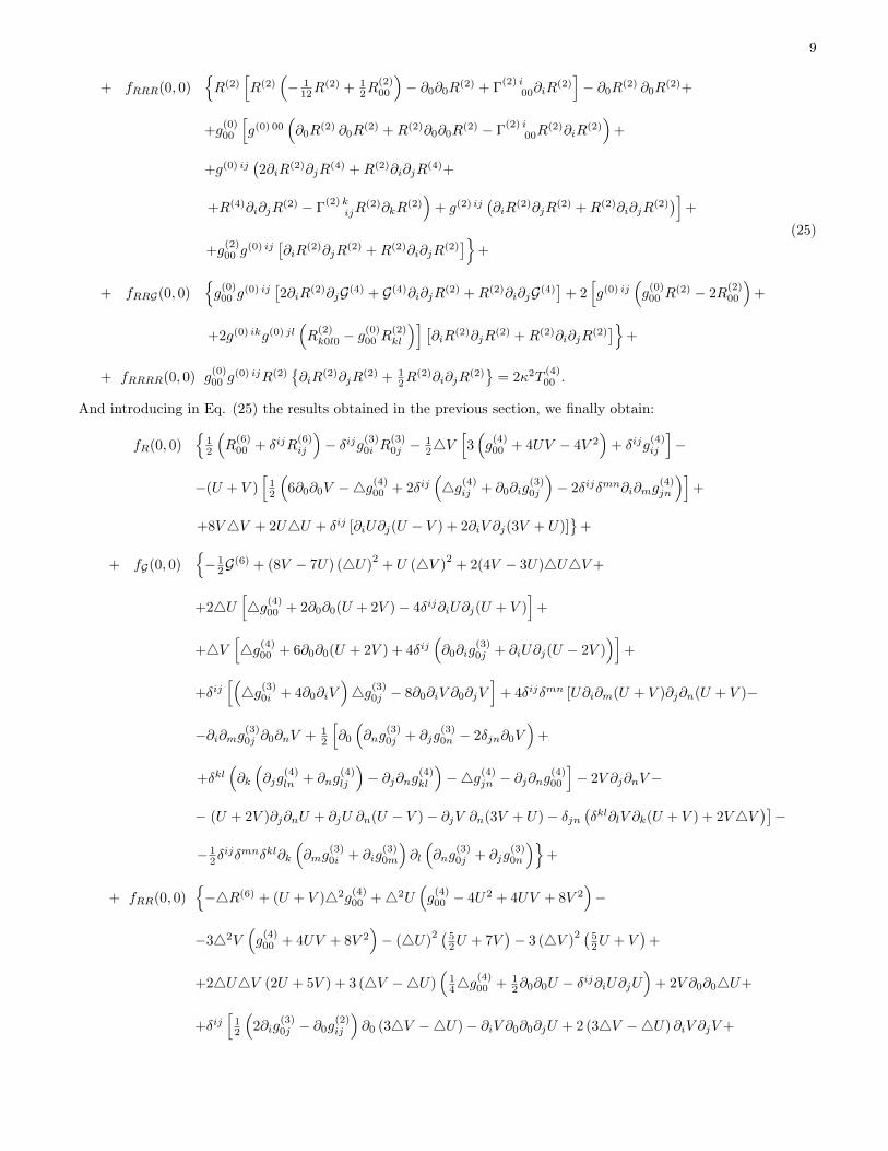
+ fRRR(0, 0){R(2)

[R(2)

(− 1

12R(2) + 1

2R(2)00

)− ∂0∂0R(2) + Γ

(2) i00∂iR

(2)]− ∂0R(2) ∂0R

(2)+

+g(0)00

[g(0) 00

(∂0R

(2) ∂0R(2) +R(2)∂0∂0R

(2) − Γ(2) i

00R(2)∂iR

(2))

+

+g(0) ij(2∂iR

(2)∂jR(4) +R(2)∂i∂jR

(4)+

+R(4)∂i∂jR(2) − Γ

(2) kijR

(2)∂kR(2))

+ g(2) ij(∂iR

(2)∂jR(2) +R(2)∂i∂jR

(2))]

+

+g(2)00 g

(0) ij[∂iR

(2)∂jR(2) +R(2)∂i∂jR

(2)]}

+

+ fRRG(0, 0){g(0)00 g

(0) ij[2∂iR

(2)∂jG(4) + G(4)∂i∂jR(2) +R(2)∂i∂jG(4)]

+ 2[g(0) ij

(g(0)00 R

(2) − 2R(2)00

)+

+2g(0) ikg(0) jl(R

(2)k0l0 − g

(0)00 R

(2)kl

)] [∂iR

(2)∂jR(2) +R(2)∂i∂jR

(2)]}

+

+ fRRRR(0, 0) g(0)00 g

(0) ijR(2){∂iR

(2)∂jR(2) + 1

2R(2)∂i∂jR

(2)}

= 2κ2T(4)00 .

(25)

And introducing in Eq. (25) the results obtained in the previous section, we finally obtain:

fR(0, 0){

12

(R

(6)00 + δijR

(6)ij

)− δijg(3)0i R

(3)0j − 1

24V[3(g(4)00 + 4UV − 4V 2

)+ δijg

(4)ij

]−

−(U + V )[12

(6∂0∂0V −4g(4)00 + 2δij

(4g(4)ij + ∂0∂ig

(3)0j

)− 2δijδmn∂i∂mg

(4)jn

)]+

+8V4V + 2U4U + δij [∂iU∂j(U − V ) + 2∂iV ∂j(3V + U)]}

+

+ fG(0, 0){− 1

2G(6) + (8V − 7U) (4U)

2+ U (4V )

2+ 2(4V − 3U)4U4V+

+24U[4g(4)00 + 2∂0∂0(U + 2V )− 4δij∂iU∂j(U + V )

]+

+4V[4g(4)00 + 6∂0∂0(U + 2V ) + 4δij

(∂0∂ig

(3)0j + ∂iU∂j(U − 2V )

)]+

+δij[(4g(3)0i + 4∂0∂iV

)4g(3)0j − 8∂0∂iV ∂0∂jV

]+ 4δijδmn [U∂i∂m(U + V )∂j∂n(U + V )−

−∂i∂mg(3)0j ∂0∂nV + 12

[∂0

(∂ng

(3)0j + ∂jg

(3)0n − 2δjn∂0V

)+

+δkl(∂k

(∂jg

(4)ln + ∂ng

(4)lj

)− ∂j∂ng(4)kl

)−4g(4)jn − ∂j∂ng

(4)00

]− 2V ∂j∂nV−

− (U + 2V )∂j∂nU + ∂jU ∂n(U − V )− ∂jV ∂n(3V + U)− δjn(δkl∂lV ∂k(U + V ) + 2V4V

)]−

− 12δijδmnδkl∂k

(∂mg

(3)0i + ∂ig

(3)0m

)∂l

(∂ng

(3)0j + ∂jg

(3)0n

)}+

+ fRR(0, 0){−4R(6) + (U + V )42g

(4)00 +42U

(g(4)00 − 4U2 + 4UV + 8V 2

)−

−342V(g(4)00 + 4UV + 8V 2

)− (4U)

2 ( 52U + 7V

)− 3 (4V )

2 ( 52U + V

)+

+24U4V (2U + 5V ) + 3 (4V −4U)(

144g

(4)00 + 1

2∂0∂0U − δij∂iU∂jU

)+ 2V ∂0∂04U+

+δij[12

(2∂ig

(3)0j − ∂0g

(2)ij

)∂0 (34V −4U)− ∂iV ∂0∂0∂jU + 2 (34V −4U) ∂iV ∂jV+

10

+24U∂iU∂jV − 12∂iV ∂j4g

(4)00 + 2g

(3)0i ∂0∂j (34V −4U) + 2∂i4U (U∂j (V − 8U)− 8V ∂jU)−

−2 (V + 3U) ∂iV ∂j (34V −4U)] +

+δijδmn[− 1

2

(2∂ig

(4)mj − ∂mg

(4)ij

)∂n (34V −4U)− g(4)im∂j∂n (34V −4U)−

−4 (2(U + V )∂i∂mU − ∂iV ∂mU) ∂j∂nU ]}+

+ fGG(0, 0){

12 (4U +4V )242U + 4 (34V −4U) (4U +4V )42V+

+4 (4U +4V ) δij [3∂i4U∂j (4U + 24V )− ∂i4V ∂j4V ] +

+4δijδmn[4 (∂i∂m(U + V )∂j∂n(U + V )) + ∂i∂mU∂j∂n

(−3 (4U)

2+ (4V )

2 − 64U4V+

+4δklδrs∂k∂r(U + V )∂l∂s(U + V ))]}

+

+ fRG(0, 0){−4G(6) + 15

2 (4U)3 − 74V (4U)

2+ 21

2 4U (4V )2

+ 212 (4V )

3 − 2 (4U +4V ) ∂0∂04U+

+42U[−4g(4)00 − 2∂0∂0U − 8(U + 3V )4U − 4(U + 2V )4V + 4δij (∂iU∂jU + ∂iV ∂jV )

]+

+42V[34g(4)00 + 6∂0∂0U − 4(3U − 2V )4U − 8(U + 7V )4V − 12δij (∂iU∂jU + ∂iV ∂jV )

]+

+4U[−42g

(4)00 + 2δij {5∂iV ∂j (34V −4U) + 8∂iU∂j4U + δmn [∂i∂mU∂j∂n(U − V )−

− ∂i∂mV ∂j∂n(U + V )]}] +

+4V[−42g

(4)00 + 2δij {3∂iV ∂j (34V −4U) + 8∂iU∂j4U + δmn [∂i∂mU∂j∂n(7U − 3V )−

3∂i∂mV ∂j∂n(U + V )]}]− δij∂iV ∂j[−3 (4U)

2+ (4V )

2 − 6 (4U) (4V ) +

+ 4δmnδkl∂m∂k (U + V ) ∂n∂l (U + V )]

+

+4(U + V )δij [∂i4V ∂j4V − 3∂i4U∂j (4U + 24V ) + 2δmn4 (∂i∂m(U + V )∂j∂n(U + V ))] +

+2δijδmn[∂i∂mU

(∂j∂n

(4g(4)00 − 4V (34V −4U) + 2∂0∂0U − 4U4U

)−

−4∂jV ∂n (34V −4U)− 8V ∂j∂n (34V −4U)) + ∂i∂m (34V −4U)(− 1

24g(4)jn −

−2V ∂j∂nV − 2U∂j∂nU − 3∂jV ∂nV + 12δkl[∂k

(∂jg

(4)ln + ∂ng

(4)lj

)− ∂j∂ng(4)kl

])]−

−8δijδmnδkl∂i∂mU∂j∂n (∂kU∂lU)}

+

+ fRRR(0, 0){42U

[124g

(4)00 + ∂0∂0U + 2(3V − U)4U − 18V4V − 2δij∂iU∂jU

]+

+42V[− 1

24g(4)00 − ∂0∂0U − 2(7V + 2U)4U + 6(7V + 3U)4V + 2δij∂iU∂jU

]−

−(

124g

(4)00 + ∂0∂04U

)(34V −4U)− 29

12 (4U)3

+ 11112 4V (4U)

2 − 574 4U (4V )

2+

+ 634 (4V )

3+ δij [∂i (34V −4U) (3 (34V −4U) ∂jV + 2 (34V +4U) ∂j (34V −4U)−

11

2∂j

(124g

(4)00 + ∂0∂0U − 2U4U

))+ 8 (34V −4U) ∂iU∂j4U

]+

+4δijδmn [∂i∂m (34V −4U) ∂j∂n (34V −4U) + (34V −4U) ∂i∂mU∂j∂nU ]}

+

+ fRRG(0, 0){42U

[−11 (4U)

2+ 25 (4V )

2+ 104U4V + 4δijδmn∂i∂m(U + V )∂j∂n(U + V )

]+

+42V[9 (4U)

2 − 39 (4V )2

+ 264U4V − 12δijδmn∂i∂m(U + V )∂j∂n(U + V )]

+

+2δij [(34V −4U) (3∂i4U∂j (4U + 24V )− ∂i4V ∂j4V )−

−∂i (34V −4U) ∂j

(−3 (4U)

2+ (4V )

2 − 64U4V+

+4δmnδkl∂m∂k(U + V )∂n∂l(U + V ))− (4U +4V ) ∂i (34V −4U) ∂j (34V −4U)

]+

+4δijδmn [∂i∂mU [∂j (34V −4U) ∂n (34V −4U) + (34V −4U) ∂j∂n (34V −4U)]−

− (34V −4U)4 (∂i∂m(U + V )∂j∂n(U + V ))]}+

+ fRRRR(0, 0){− 1

2 (34V −4U)2 (

342V −42U)− δij (34V −4U) ∂i (34V −4U) ∂j (34V −4U)

}=

= 2κ2{ρ[v4 − 3Uv2 + 4U2 + 2g

(4)00 + 2g

(3)0i v

i + Π(v2 − 4U)]

+ p(v2 − 2U

)}

(26)

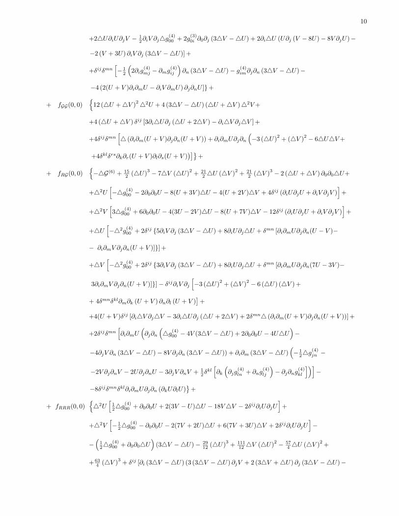
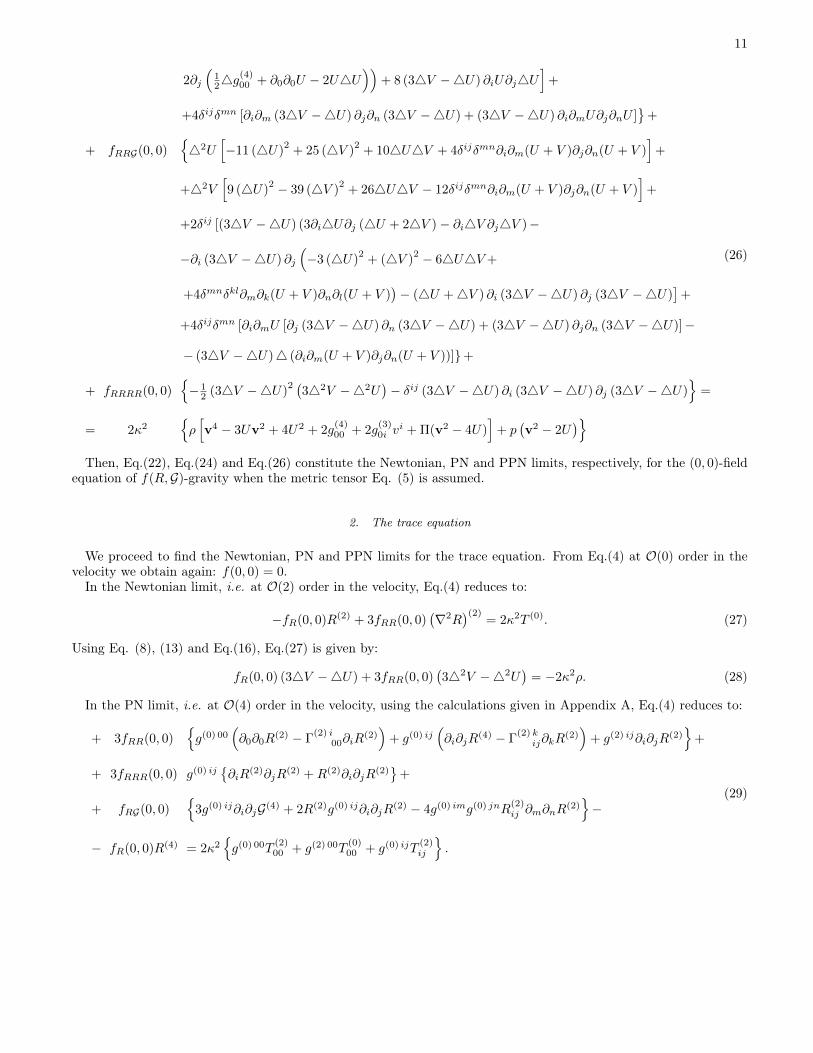
Then, Eq.(22), Eq.(24) and Eq.(26) constitute the Newtonian, PN and PPN limits, respectively, for the (0, 0)-fieldequation of f(R,G)-gravity when the metric tensor Eq. (5) is assumed.

2. The trace equation

We proceed to find the Newtonian, PN and PPN limits for the trace equation. From Eq.(4) at O(0) order in thevelocity we obtain again: f(0, 0) = 0.

In the Newtonian limit, i.e. at O(2) order in the velocity, Eq.(4) reduces to:

−fR(0, 0)R(2) + 3fRR(0, 0)(∇2R

)(2)= 2κ2T (0). (27)

Using Eq. (8), (13) and Eq.(16), Eq.(27) is given by:

fR(0, 0) (34V −4U) + 3fRR(0, 0)(342V −42U

)= −2κ2ρ. (28)

In the PN limit, i.e. at O(4) order in the velocity, using the calculations given in Appendix A, Eq.(4) reduces to:

+ 3fRR(0, 0){g(0) 00

(∂0∂0R

(2) − Γ(2) i

00∂iR(2))

+ g(0) ij(∂i∂jR

(4) − Γ(2) k

ij∂kR(2))

+ g(2) ij∂i∂jR(2)}

+

+ 3fRRR(0, 0) g(0) ij{∂iR

(2)∂jR(2) +R(2)∂i∂jR

(2)}

+

+ fRG(0, 0){

3g(0) ij∂i∂jG(4) + 2R(2)g(0) ij∂i∂jR(2) − 4g(0) img(0) jnR

(2)ij ∂m∂nR

(2)}−

− fR(0, 0)R(4) = 2κ2{g(0) 00T

(2)00 + g(2) 00T

(0)00 + g(0) ijT

(2)ij

}.

(29)

12

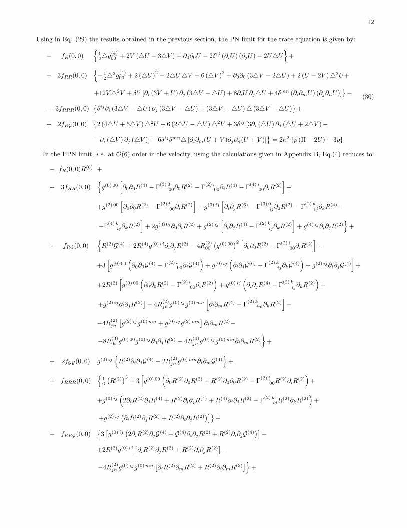
Using in Eq. (29) the results obtained in the previous section, the PN limit for the trace equation is given by:

− fR(0, 0){

124g

(4)00 + 2V (4U − 34V ) + ∂0∂0U − 2δij (∂iU) (∂jU)− 2U4U

}+

+ 3fRR(0, 0){− 1

242g

(4)00 + 2 (4U)

2 − 24U 4V + 6 (4V )2

+ ∂0∂0 (34V − 24U) + 2 (U − 2V )42U+

+12V42V + δij [∂i (3V + U) ∂j (34V −4U) + 8∂iU ∂j4U + 4δmn (∂i∂mU) (∂j∂nU)]}−

− 3fRRR(0, 0){δij∂i (34V −4U) ∂j (34V −4U) + (34V −4U)4 (34V −4U)

}+

+ 2fRG(0, 0){

2 (44U + 54V )42U + 6 (24U −4V )42V + 3δij [3∂i (4U) ∂j (4U + 24V )−

−∂i (4V ) ∂j (4V )]− 6δijδmn4 [∂i∂m(U + V )∂j∂n(U + V )]}

= 2κ2 {ρ (Π− 2U)− 3p}

(30)

In the PPN limit, i.e. at O(6) order in the velocity, using the calculations given in Appendix B, Eq.(4) reduces to:

− fR(0, 0)R(6) +

+ 3fRR(0, 0){g(0) 00

[∂0∂0R

(4) − Γ(3) 0

00∂0R(2) − Γ

(2) i00∂iR

(4) − Γ(4) i

00∂iR(2)]

+

+g(2) 00[∂0∂0R

(2) − Γ(2) i

00∂iR(2)]

+ g(0) ij[∂i∂jR

(6) − Γ(3) 0

ij∂0R(2) − Γ

(2) kij∂kR

(4)−

−Γ(4) k

ij∂kR(2)]

+ 2g(3) 0i∂0∂iR(2) + g(2) ij

[∂i∂jR

(4) − Γ(2) k

ij∂kR(2)]

+ g(4) ij∂i∂jR(2)}

+

+ fRG(0, 0){R(2)G(4) + 2R(4)g(0) ij∂i∂jR

(2) − 4R(2)00

(g(0) 00

)2 [∂0∂0R

(2) − Γ(2) i

00∂iR(2)]

+

+3[g(0) 00

(∂0∂0G(4) − Γ

(2) i00∂iG(4)

)+ g(0) ij

(∂i∂jG(6) − Γ

(2) kij∂kG(4)

)+ g(2) ij∂i∂jG(4)

]+

+2R(2)[g(0) 00

(∂0∂0R

(2) − Γ(2) i

00∂iR(2))

+ g(0) ij(∂i∂jR

(4) − Γ(2) k

ij∂kR(2))

+

+g(2) ij∂i∂jR(2)]− 4R

(2)jn g

(0) ijg(0)mn[∂i∂mR

(4) − Γ(2) k

im∂kR(2)]−

−4R(2)jn

[g(2) ijg(0)mn + g(0) ijg(2)mn

]∂i∂mR

(2)−

−8R(3)0i g

(0) 00g(0) ij∂0∂jR(2) − 4R

(4)jn g

(0) ijg(0)mn∂i∂mR(2)}

+

+ 2fGG(0, 0) g(0) ij{R(2)∂i∂jG(4) − 2R

(2)jn g

(0)mn∂i∂mG(4)}

+

+ fRRR(0, 0){

16

(R(2)

)3+ 3

[g(0) 00

(∂0R

(2)∂0R(2) +R(2)∂0∂0R

(2) − Γ(2) i

00R(2)∂iR

(2))

+

+g(0) ij(

2∂iR(2)∂jR

(4) +R(2)∂i∂jR(4) +R(4)∂i∂jR

(2) − Γ(2) k

ijR(2)∂kR

(2))

+

+g(2) ij(∂iR

(2)∂jR(2) +R(2)∂i∂jR

(2))]}

+

+ fRRG(0, 0){

3[g(0) ij

(2∂iR

(2)∂jG(4) + G(4)∂i∂jR(2) +R(2)∂i∂jG(4))]

+

+2R(2)g(0) ij[∂iR

(2)∂jR(2) +R(2)∂i∂jR

(2)]−

−4R(2)jn g

(0) ijg(0)mn[∂iR

(2)∂mR(2) +R(2)∂i∂mR

(2)]}

+

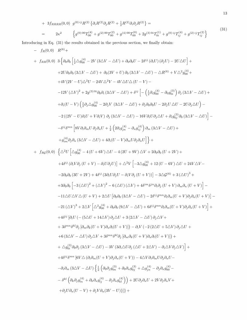
13

+ 3fRRRR(0, 0) g(0) ijR(2){∂iR

(2)∂jR(2) + 1

2R(2)∂i∂jR

(2)}

=

= 2κ2{g(0) 00T

(4)00 + g(2) 00T

(2)00 + g(4) 00T

(0)00 + 2g(3) 0iT

(1)0i + g(0) ijT

(4)ij + g(2) ijT

(2)ij

} (31)

Introducing in Eq. (31) the results obtained in the previous section, we finally obtain:

− fR(0, 0) R(6)+

+ fRR(0, 0) 3{∂0∂0

[124g

(4)00 − 2V (34V −4U) + ∂0∂0U − 2δij (∂iU) (∂jU)− 2U4U

]+

+2U∂0∂0 (34V −4U) + ∂0(3V + U) ∂0 (34V −4U)−4R(6) + V42g(4)00 +

+4V (2V − U)42U − 24V42V − 4V4U4 (U − V )−

−12V (4V )2

+ 2g(3) 0i∂0∂i (34V −4U) + δij[−(

12∂ig

(4)00 − ∂0g

(3)0i

)∂j (34V −4U) +

+∂i(U − V )(

12∂j4g

(4)00 − 2∂jV (34V −4U) + ∂j∂0∂0U − 2∂jU 4U − 2U∂j4U

)−

−2 ((2V − U)∂iU + V ∂iV ) ∂j (34V −4U)− 16V ∂iU∂j4U + ∂ig(3)0j ∂0 (34V −4U)

]−

−δijδmn[8V ∂i∂mU ∂j∂nU + 1

2

(2∂ig

(4)jn − ∂ng

(4)ij

)∂m (34V −4U) +

+g(4)im∂j∂n (34V −4U) + 4∂i(U − V )∂mU∂j∂nU

]}+

+ fRG(0, 0){42U

[4g(4)00 − 4 (U + 6V )4U − 4 (2U + 9V )4V + 2∂0∂0 (U + 2V ) +

+4δij (∂iV ∂j (U + V )− ∂iU∂jU)]

+42V[−34g(4)00 + 12 (U − 6V )4U + 24V4V−

−2∂0∂0 (3U + 2V ) + 4δij (3∂iU∂jU − ∂iV ∂j (U + V ))]− 34G(6) + 3 (4U)

3+

+3∂0∂0

[−3 (4U)

2+ (4V )

2 − 6 (4U) (4V ) + 4δimδjn∂i∂j (U + V ) ∂m∂n (U + V )]−

−114U4V4 (U + V ) + 24U[∂0∂0 (34V −4U)− 2δijδmn∂i∂m(U + V )∂j∂n(U + V )

]−

−21 (4V )3

+ 24V[42g

(4)00 + ∂0∂0 (94V −4U) + 6δijδmn∂i∂m(U + V )∂j∂n(U + V )

]+

+4δij [∂iU (− (54U + 144V ) ∂j4U + 3 (24V −4U) ∂j4V+

+ 3δmnδkl∂j [∂m∂k(U + V )∂n∂l(U + V )])− ∂iV (−2 (24U + 54V ) ∂j4U +

+6 (34V −4U) ∂j4V + 3δmnδkl∂j [∂m∂k(U + V )∂n∂l(U + V )])

+

+ 4g(3)0i ∂0∂j (34V −4U)− 3V (3∂i4U∂j (4U + 24V )− ∂i4V ∂j4V )]

+

+4δijδmn [6V4 (∂i∂m(U + V )∂j∂n(U + V ))− 44V ∂i∂mU∂j∂nU−

−∂i∂m (34V −4U){

12

(∂0∂jg

(3)0n + ∂0∂ng

(3)0j +4g(4)jn − ∂j∂ng

(4)00 −

− δkl(∂k∂jg

(4)ln + ∂k∂ng

(4)lj − ∂j∂ng

(4)kl

))+ 2U∂j∂nU + 2V ∂j∂nV+

+∂jU∂n(U − V ) + ∂jV ∂n(3V − U)}]}+

14

+ fGG(0, 0) 2 (4U −4V )4{−3 (4U)

2+ (4V )

2 − 6 (4U) (4V ) + 4δimδjn∂i∂j (U + V ) ∂m∂n (U + V )}

+

+ fRRR(0, 0){− 3

2 (34V −4U)42g(4)00 − 37

6 (4U)3

+ 512 (4U)

24V − 812 4U (4V )

2+ 117

2 (4V )3

+

+342U[124g

(4)00 + ∂0∂0U − 2(U + 3V ) (34V −4U)− 2δij∂iU∂jU − 2U4U

]+

+942V[− 1

24g(4)00 − ∂0∂0U + 6V (34V −4U) + 2δij∂iU∂jU + 2U4U

]+

+3 (34V −4U) ∂0∂0 (34V − 24U) + 3∂0 (34V −4U) ∂0 (34V −4U) +

+3δij[8 (34V −4U) ∂iU∂j4U +

(−∂i4g(4)00 + (34V −4U) ∂i (U + 7V ) +

+6V ∂i (34V −4U)− 2∂i∂0∂0U + 44U∂iU + 4U∂i4U) ∂j (34V −4U)] +

+12δijδmn [(34V −4U) ∂i∂mU ∂j∂nU + 2∂iU∂m (34V −4U) ∂j∂nU ]}

+

+ fRRG(0, 0){42U

[−25 (4U)

2+ 63 (4V )

2+ 104U4V + 12 δijδmn ∂i∂m(U + V ) ∂j∂n(U + V )

]+

+342V[(4U)

2 − 15 (4V )2

+ 464U4V − 12 δijδmn ∂i∂m(U + V ) ∂j∂n(U + V )]

+

+2δij [3 (34V −4U) (3∂i4U∂j4U − ∂i4V ∂j4V + 6∂i4U∂j4V )−

−3∂i (34V −4U) ∂j

(−3 (4U)

2+ (4V )

2 − 6 (4U) (4V ) + +

+4δimδjn ∂i∂j (U + V ) ∂m∂n (U + V ))

+ (54V −4U) ∂i (34V −4U) ∂j (34V −4U)]−

−12δijδmn (34V −4U)4 [∂i∂j (U + V ) ∂m∂n (U + V )]}−

− fRRRR(0, 0) 3 (34V −4U){∂i (34V −4U) ∂j (34V −4U) + 1

2 (34V −4U)(342V −42U

)}=

= 2κ2{ρ[−v2 (U + 2V ) + g

(4)00 + 2g

(3)0i v

i − 2UΠ]− 2Up

}.

(32)Then, Eq.(28), Eq.(30) and Eq.(32) constitute the Newtonian, PN and PPN limit, respectively, for the trace

equation of f(R,G)- gravity when the metric tensor given by Eq. (5) is assumed.

III. SOLVING THE FIELD EQUATIONS IN THE NEWTONIAN LIMIT

Our aim is now to solve the system of equations for the Newtonian limit of f(R,G)- gravity, i.e. the systemconstituted by Eq.(22) and Eq.(28), in the most general way. In order to do this, we will search for solutions in termsof Green’s functions (see [43]).

We start by considering the set of equations given by Eq.(22) and Eq.(28), this is:

fR(0, 0) (34V +4U) + 2fRR(0, 0)(342V −42U

)= −4κ2ρ ,

fR(0, 0) (34V −4U) + 3fRR(0, 0)(342V −42U

)= −2κ2ρ .

(33)

By introducing the new auxiliary functions A = fR(0, 0)(3V + U) and B = 2fRR(0, 0) (3V − U), we can write Eq.(33) as:

−4κ2ρ = 4A+42B ,

−4κ2ρ = fR(0,0)fRR(0,0)4B + 342B .

(34)

15

Considering now the new function Φ = A+4B, Eq. (34) reduces to:

−4κ2ρ = 4Φ ,

−4κ2ρ = fR(0,0)fRR(0,0)4B + 342B .

(35)

It is important to remark that Eq. (35) is a set of uncoupled equations. We are interested in the solution of thesecond equation in Eq. (35) in terms of the Green’s function G(x,x’) defined by:

B = −4κ2C

∫d3x’G(x,x’) , ρ(x’) (36)

where C is a constant, which is introduced for dimensional reasons. Now the set of equations given by Eq. (35) isequivalent to:

−4κ2ρ = 4Φ ,

1C δ(x− x’) = fR(0,0)

fRR(0,0)4xG(x,x’) + 342xG(x,x’) ,(37)

where δ(x − x’) is the three-dimensional Dirac δ-function. The general solutions of Eqs.(33) for U(x) and V (x), interms of the Green’s function G(x,x’) and the function Φ(x), are:

U(x) = 12fR(0, 0)

Φ(x) + 2κ2C

(4x

fR(0, 0)+ 1

2fRR(0, 0)

)∫d3x’G(x,x’)ρ(x’) ,

V (x) = 16fR(0, 0)

Φ(x) + 23κ

2C

(4x

fR(0, 0)− 1

2fRR(0, 0)

)∫d3x’G(x,x’)ρ(x’) .

(38)

In summary, the functions U(x) and V (x), which are related with g(2)00 and g(2)ij , respectively, by Eq.(5) have beenfound in terms of the Green’s function G(x,x’) and the function Φ(x), giving in this way a general solution to theNewtonian limit for f(R,G) -gravity theories.

IV. THE WEAK FIELD LIMIT IN TWO SPECIAL CASES: f(R) AND f(G) GRAVITIES

The results obtained previously will be used for two special cases: f(R)- gravity and f(G)-gravity, respectively.

A. f(R) gravity

The starting action is given by:

S =

∫d4x√−g(

1

2κ2f(R) + Lm

). (39)

In order to obtain the Newtonian, PN and PPN limits for this theory we will use the equations of the previoussection considering the change: f(R,G)→ f(R). The field equations for f(R)- gravity are obtained from Eq.(3):

−1

2gµνf(R) + f ′(R)Rµν + gµν∇2f ′(R)−∇µ∇νf ′(R) = 2κ2Tµν , (40)

where primes denote the derivative with respect to Ricci scalar, while the trace equation is obtained from Eq.(4):

−2f(R) + f ′(R)R+ 3∇2f ′(R) = 2κ2T. (41)

Before analyzing the Newtonian, PN and PPN limits for this theory, it is important to remark that at the lowestorder in the velocity, i.e. O(0)-order, from Eq.(40) and Eq.(41), we obtain: f(0) = 0.

16

1. The Newtonian limit

The Newtonian limit of f(R)-gravity corresponds to O(2)-order for Eq.(40) and Eq.(41).The (0, 0)-field equation for f(R)- gravity at Newtonian order can be obtained from Eq. (22) and it is given by:

f ′(0) (34V +4U) + 2f ′′(0)(342V −42U

)= −4κ2ρ. (42)

The trace equation for f(R) modified gravity at Newtonian order can be obtained from Eq.(28) and it is given by:

f ′(0) (34V −4U) + 3f ′′(0)(342V −42U

)= −2κ2ρ. (43)

2. The Post Newtonian limit

In this case, the aim is to obtain Eq.(40) and Eq.(41) at O(4)-order in the velocity.For the (0, 0)-field equation, we use Eq.(24). For f(R)-gravity it reduces to:

f ′(0){

144g

(4)00 + 3(U + V )4V + V4U + 1

2∂0∂0U − δij∂iU∂jU

}+

+ f ′′(0){− 1

242g

(4)00 + 15

4 (4V )2 − 7

24U4V + 114 (4U)

2+ 6(U + 2V )42V − 4V42U − ∂0∂04U+

+ δij [3∂iV ∂j (34V −4U) + 8∂iU ∂j4U + 4δmn∂i∂mU ∂j∂nU ]}−

− f ′′′(0){δij∂i (34V −4U) ∂j (34V −4U) + (34V −4U)4 (34V −4U)

}= 2κ2ρ

(Π + v2 − 4U

).

(44)

While for the trace equation, Eq.(30) gives:

− f ′(0){

124g

(4)00 + 2V (4U − 34V ) + ∂0∂0U − 2δij (∂iU) (∂jU)− 2U4U

}+

+ 3f ′′(0){− 1

242g

(4)00 + 2 (4U)

2 − 24U 4V + 6 (4V )2

+ ∂0∂0 (34V − 24U) + 2 (U − 2V )42U+

+12V42V + δij [∂i (3V + U) ∂j (34V −4U) + 8∂iU ∂j4U + 4δmn (∂i∂mU) (∂j∂nU)]}−

− 3f ′′′(0){δij∂i (34V −4U) ∂j (34V −4U) + (34V −4U)4 (34V −4U)

}= 2κ2 {ρ (Π− 2U)− 3p}

(45)

3. The Parameterized Post Newtonian limit

Finally, the PPN limit corresponds to O(6)-order for Eq.(40) and Eq.(41).For the (0, 0)-field equation we obtain from Eq.(26) the following result:

f ′(0){

12

(R

(6)00 + δijR

(6)ij

)− δijg(3)0i R

(3)0j − 1

24V[3(g(4)00 + 4UV − 4V 2

)+ δijg

(4)ij

]−

−(U + V )[12

(6∂0∂0V −4g(4)00 + 2δij

(4g(4)ij + ∂0∂ig

(3)0j

)− 2δijδmn∂i∂mg

(4)jn

)]+

+8V4V + 2U4U + δij [∂iU∂j(U − V ) + 2∂iV ∂j(3V + U)]}

+

+ f ′′(0){−4R(6) + (U + V )42g

(4)00 +42U

(g(4)00 − 4U2 + 4UV + 8V 2

)− 342V

(g(4)00 + 4UV + 8V 2

)−

− (4U)2 ( 5

2U + 7V)− 3 (4V )

2 ( 52U + V

)+ 24U4V (2U + 5V ) +

+3 (4V −4U)(

144g

(4)00 + 1

2∂0∂0U − δij∂iU∂jU

)+ 2V ∂0∂04U+

+δij[12

(2∂ig

(3)0j − ∂0g

(2)ij

)∂0 (34V −4U)− ∂iV ∂0∂0∂jU + 2 (34V −4U) ∂iV ∂jV+

+24U∂iU∂jV − 12∂iV ∂j4g

(4)00 + 2g

(3)0i ∂0∂j (34V −4U) + 2∂i4U (U∂j (V − 8U)− 8V ∂jU)−

17

−2 (V + 3U) ∂iV ∂j (34V −4U)] + δijδmn[− 1

2

(2∂ig

(4)mj − ∂mg

(4)ij

)∂n (34V −4U)−

−g(4)im∂j∂n (34V −4U)− 4 (2(U + V )∂i∂mU − ∂iV ∂mU) ∂j∂nU]}

+

+ f ′′′(0){42U

[124g

(4)00 + ∂0∂0U + 2(3V − U)4U − 18V4V − 2δij∂iU∂jU

]+

+42V[− 1

24g(4)00 − ∂0∂0U − 2(7V + 2U)4U + 6(7V + 3U)4V + 2δij∂iU∂jU

]−

−(

124g

(4)00 + ∂0∂04U

)(34V −4U)− 29

12 (4U)3

+ 634 (4V )

3+ 111

12 4V (4U)2 − 57

4 4U (4V )2

+

+δij [∂i (34V −4U) (3 (34V −4U) ∂jV + 2 (34V +4U) ∂j (34V −4U)−

2∂j

(124g

(4)00 + ∂0∂0U − 2U4U

))+ 8 (34V −4U) ∂iU∂j4U

]+

+4δijδmn [∂i∂m (34V −4U) ∂j∂n (34V −4U) + (34V −4U) ∂i∂mU∂j∂nU ]}

+

+ f ′′′′(0){− 1

2 (34V −4U)2 (

342V −42U)− δij (34V −4U) ∂i (34V −4U) ∂j (34V −4U)

}=

= 2κ2{ρ[v4 − 3Uv2 + 4U2 + 2g

(4)00 + 2g

(3)0i v

i + Π(v2 − 4U)]

+ p(v2 − 2U

)}

(46)

And Eq.(32) implies that the trace equation is given by:

− f ′(0)R(6) +

+ 3f ′′(0){∂0∂0

[124g

(4)00 − 2V (34V −4U) + ∂0∂0U − 2δij (∂iU) (∂jU)− 2U4U

]+

+2U∂0∂0 (34V −4U) + ∂0(3V + U) ∂0 (34V −4U)−4R(6) + V42g(4)00 +

+4V (2V − U)42U − 24V42V − 4V4U4 (U − V )− 12V (4V )2

+

+2g(3) 0i∂0∂i (34V −4U) + δij[−(

12∂ig

(4)00 − ∂0g

(3)0i

)∂j (34V −4U) +

+∂i(U − V )(

12∂j4g

(4)00 − 2∂jV (34V −4U) + ∂j∂0∂0U − 2∂jU 4U − 2U∂j4U

)−

−2 ((2V − U)∂iU + V ∂iV ) ∂j (34V −4U)− 16V ∂iU∂j4U + ∂ig(3)0j ∂0 (34V −4U)

]−

−δijδmn[8V ∂i∂mU ∂j∂nU + 1

2

(2∂ig

(4)jn − ∂ng

(4)ij

)∂m (34V −4U) +

+g(4)im∂j∂n (34V −4U) + 4∂i(U − V )∂mU∂j∂nU

]}+

+ f ′′′(0){− 3

2 (34V −4U)42g(4)00 + 342U

[124g

(4)00 + ∂0∂0U − 2(U + 3V ) (34V −4U)−

−2δij∂iU∂jU − 2U4U]− 37

6 (4U)3

+ 512 (4U)

24V − 812 4U (4V )

2+ 117

2 (4V )3

+

+942V[− 1

24g(4)00 − ∂0∂0U + 6V (34V −4U) + 2δij∂iU∂jU + 2U4U

]−

+3 (34V −4U) ∂0∂0 (34V − 24U) + 3∂0 (34V −4U) ∂0 (34V −4U) +

+3δij[8 (34V −4U) ∂iU∂j4U +

(−∂i4g(4)00 + (34V −4U) ∂i (U + 7V ) +

18

+6V ∂i (34V −4U)− 2∂i∂0∂0U + 44U∂iU + 4U∂i4U) ∂j (34V −4U)] +

+12δijδmn [(34V −4U) ∂i∂mU ∂j∂nU + 2∂iU∂m (34V −4U) ∂j∂nU ]}−

− 3f ′′′′(0) (34V −4U){∂i (34V −4U) ∂j (34V −4U) + 1

2 (34V −4U)(342V −42U

)}=

= 2κ2{ρ[−v2 (U + 2V ) + g

(4)00 + 2g

(3)0i v

i − 2UΠ]− 2Up

}.

(47)

Summing up, the Newtonian limit of f(R) modified gravity theories is given by Eq.(42) and Eq.(43); the PN limitis given by Eq.(44) and Eq.(45); and the PPN limit is given by Eq.(46) and Eq.(47), respectively.

B. f(G) gravity

Let us consider now the following action:

S =

∫d4x√−g{

1

2κ2[R+ f(G)] + Lmatter

}, (48)

where standard GR is obviously recovered for f(G)→ 0. We proceed in the same way as for f(R)-gravity, but in thiscase we have f(R,G)→ R+ f(G).

The field equations can be directly obtained from Eq. (3):

−1

2gµν (R+ f(G)) +Rµν + 2f ′(G)RRµν − 4f ′(G)RµρR

ρν + 2f ′(G)RαβρµR

αβρν − 4f ′(G)RµρνσR

ρσ+

+2gµνR∇2f ′(G)− 4gµνRρσ∇ρ∇σf ′(G)− 2R∇µ∇νf ′(G)− 4Rµν∇2f ′(G) + 4Rνρ∇ρ∇µf ′(G) + 4Rµρ∇ρ∇νf ′(G)+

+4Rµρνσ∇ρ∇σf ′(G) = 2κ2Tµν , (49)

while the trace equation is obtained from Eq.(4):

−R− 2f(G) + 2f ′(G)G + 2R∇2f ′(G)− 4Rρσ∇ρ∇σf ′(G) = 2κ2T. (50)

From the lowest order we obtain again: f(0) = 0.

1. The Newtonian limit

In this case, the (0, 0)-field equation obtained from Eq.(22) is given by:

4U + 34V = −4κ2ρ. (51)

While the trace equation can be obtained from Eq.(28) and it reduces to:

4U − 34V = 2κ2ρ. (52)

2. The Post Newtonian limit

The PN limit for the (0, 0)-field equation can be calculated from Eq.(24) and it reduces to:

144g

(4)00 + 3(U + V )4V + V4U + 1

2∂0∂0U − δij∂iU∂jU+

+ f ′(0){− 1

2 (4U −4V )2

+ 2δimδjn∂i∂j (U − V ) ∂m∂n (U − V )}

= 2κ2ρ(Π + v2 − 4U

) (53)

For the case of the trace equation, Eq.(30) reduces to:

− 124g

(4)00 + 2V (4U − 34V ) + ∂0∂0U − 2δij (∂iU) (∂jU)− 2U4U = 2κ2 {ρ (Π− 2U)− 3p} (54)

19

3. The Parameterized Post Newtonian limit

The PPN limit for the (0, 0)-field equation is obtained from Eq.(24) and can be written as:

12

(R

(6)00 + δijR

(6)ij

)− δijg(3)0i R

(3)0j − 1

24V[3(g(4)00 + 4UV − 4V 2

)+ δijg

(4)ij

]+

+δij [∂iU∂j(U − V ) + 2∂iV ∂j(3V + U)] + 8V4V + 2U4U−

−(U + V )[12

(6∂0∂0V −4g(4)00 + 2δij

(4g(4)ij + ∂0∂ig

(3)0j

)− 2δijδmn∂i∂mg

(4)jn

)]+

+ f ′(0){− 1

2G(6) + (8V − 7U) (4U)

2+ U (4V )

2+ 2(4V − 3U)4U4V + 24U

[4g(4)00 + 2∂0∂0(U + 2V )−

−4δij∂iU∂j(U + V )]

+4V[4g(4)00 + 6∂0∂0(U + 2V ) + 4δij

(∂0∂ig

(3)0j + ∂iU∂j(U − 2V )

)]+

+δij[(4g(3)0i + 4∂0∂iV

)4g(3)0j − 8∂0∂iV ∂0∂jV

]+ 4δijδmn [U∂i∂m(U + V )∂j∂n(U + V )−

−∂i∂mg(3)0j ∂0∂nV + 12

[∂0

(∂ng

(3)0j + ∂jg

(3)0n − 2δjn∂0V

)+ δkl

(∂k

(∂jg

(4)ln + ∂ng

(4)lj

)− ∂j∂ng(4)kl

)−

− 4g(4)jn − ∂j∂ng(4)00

]− 2V ∂j∂nV − (U + 2V )∂j∂nU + ∂jU ∂n(U − V )− ∂jV ∂n(3V + U)−

−δjn(δkl∂lV ∂k(U + V ) + 2V4V

)]12δijδmnδkl∂k

(∂mg

(3)0i + ∂ig

(3)0m

)∂l

(∂ng

(3)0j + ∂jg

(3)0n

)}+

+ f ′′(0){

12 (4U +4V )242U + 4 (34V −4U) (4U +4V )42V+

+4 (4U +4V ) δij [3∂i4U∂j (4U + 24V )− ∂i4V ∂j4V ] +

+4δijδmn[4 (∂i∂m(U + V )∂j∂n(U + V )) + ∂i∂mU∂j∂n

(−3 (4U)

2+ (4V )

2 − 64U4V+

+4δklδrs∂k∂r(U + V )∂l∂s(U + V ))]}

=

= 2κ2{ρ[v4 − 3Uv2 + 4U2 + 2g

(4)00 + 2g

(3)0i v

i + Π(v2 − 4U)]

+ p(v2 − 2U

)}.

(55)

And for the trace equation, Eq.(32) reduces to:

−R(6) + 2f ′′(0) (4U −4V )4{−3 (4U)

2+ (4V )

2 − 6 (4U) (4V ) + 4δimδjn∂i∂j (U + V ) ∂m∂n (U + V )}

=

= 2κ2{ρ[−v2 (U + 2V ) + g

(4)00 + 2g

(3)0i v

i − 2UΠ]− 2Up

}. (56)

Summarizing, the Newtonian limit of f(G)- gravity theories is given by Eq.(51) and Eq.(52); the PN limit is givenby Eq.(53) and Eq.(54); and the PPN limit is given by Eq.(55) and Eq.(56), respectively.

V. CONCLUSIONS

Achieving the weak field limit is the straightforward approach to compare any theory of gravity with GR. In a widesense, this is the main consistency check in order to establish if a given theory of gravity can reproduce or not theclassical experimental tests of GR and then address further phenomena and/or anomalous experimental data.

This philosophy has recently become a paradigm due to the fact that alternative theories of gravity and extendedtheories of gravity are aimed to reproduce GR results from one side (Solar System and laboratory scales) and address

20

a huge amount of phenomena starting from quantization and renormalization of gravitational interaction (ultravioletscales) up to the large scale structure and the cosmological accelerated behavior of the Hubble flow (infrared scales).

The weak field limit approach is based on the theory of perturbations in terms of powers c−2 where c is the speedof light. Newtonian, Post Newtonian and further limits strictly depends on the accuracy of such a development andon the identification of suitable parameters that have to be confronted with the experiments.

Here we have considered a wide class of these theories, specifically the f(R,G) gravity consisting of analytic modelsthat are functions of the Ricci scalar R and the Gauss-Bonnet invariant G. In this context, we have worked out theNewtonian, the Post Newtonian and the Parameterized Post Newtonian limits.

The main result of the approach is that new features come out with respect to GR and, due to fourth-order fieldequations, at least two gravitational potentials have to be considered. This fact could be extremely important in orderto deal with realistic self-gravitating structures since they could results more stable and without singularities.

Specifically, we found some general solutions in the Newtonian limit and developed in details (Newtonian, PostNewtonian e Parameterized Post Newtonian limits) the cases of f(R) gravity and R + f(G) gravity. In particular,the presence of the topological terms seems relevant to remove singularities and give rise to stable structures. In aforthcoming paper, we will phenomenologically confront these theoretical results with experimental data.

Acknowledgements. MDL acknowledges the support of INFN Sez. di Napoli (Iniziative Specifiche TEONGRAVand QGSKY). AJLR acknowledges a JAE fellowship from CSIC (Barcelona, Spain).

21

Appendix A: The Post Newtonian limit

In this appendix, we present the calculations needed to obtain the PN limit for the field equations and the traceequation. First, we write some calculations that will be needed after:

(∇2f∗(R,G)

)(2)= g(0) ijf∗R(0, 0)∂i∂jR

(2)

(∇2f∗(R,G)

)(4)= g(0) 00

{f∗R(0, 0)∂0∂0R

(2) − Γ(2) i

00f∗R(0, 0)∂iR

(2)}

+

+g(0) ij{f∗RR(0, 0)∂iR

(2)∂jR(2) + f∗R(0, 0)∂i∂jR

(4) + f∗RR(0, 0)R(2)∂i∂jR(2)+

+f∗G(0, 0)∂i∂jG(4) − Γ(2) k

ijf∗R(0, 0)∂kR

(2)}

+ g(2) ijf∗R(0, 0)∂i∂jR(2)

(∇2f∗(R,G)

)(6)= g(0) 00

{f∗RR(0, 0)∂0R

(2)∂0R(2) + f∗R(0, 0)∂0∂0R

(4) + f∗RR(0, 0)R(2)∂0∂0R(2)+

+f∗G(0, 0)∂0∂0G(4) − Γ(3) 0

00f∗R(0, 0)∂0R

(2) − Γ(4) i

00f∗R(0, 0)∂iR

(2)−

−Γ(2) i

00

[f∗R(0, 0)∂iR

(4) + f∗RR(0, 0)R(2)∂iR(2) + f∗G(0, 0)∂iG(4)

]}+

+g(2) 00{f∗R(0, 0)∂0∂0R

(2) − Γ(2) i

00f∗R(0, 0)∂iR

(2)}

+

+2g(3) 0if∗R(0, 0)∂0∂iR(2)+

+g(0) ij{

2f∗RR(0, 0)∂iR(2)∂jR

(4) + f∗RRR(0, 0)R(2)∂iR(2)∂jR

(2) + 2f∗RG(0, 0)∂iR(2)∂jG(4)+

+f∗R(0, 0)∂i∂jR(6) + f∗RR(0, 0)R(2)∂i∂jR

(4)+

+[12f∗RRR(0, 0)R(2) 2 + f∗RR(0, 0)R(4) + f∗RG(0, 0)G(4)

]∂i∂jR

(2)+

+f∗G(0, 0)∂i∂jG(6) + f∗RG(0, 0)R(2)∂i∂jG(4) − Γ(3) 0

ijf∗R(0, 0)∂0R

(2)−

−Γ(2) k

ij

[f∗R(0, 0)∂kR

(4) + f∗RR(0, 0)R(2)∂kR(2) + f∗G(0, 0)∂kG(4)

]−

−Γ(4) k

ijf∗R(0, 0)∂kR

(2)}

+

+g(2) ij{f∗RR(0, 0)∂iR

(2)∂jR(2) + f∗R(0, 0)∂i∂jR

(4) + f∗RR(0, 0)R(2)∂i∂jR(2)+

+f∗G(0, 0)∂i∂jG(4) − Γ(2) k

ijf∗R(0, 0)∂kR

(2)}

+

+g(4) ijf∗R(0, 0)∂i∂jR(2)

(Rαβρ0R

αβρ0

)(4)= 2δijδmn (∂i∂mU) (∂j∂nU)

(Rαβρ0R

αβρ0

)(6)= 44U

(∂0∂0V + δij∂iU ∂jV

)+ 2δijδmn∂i∂mU

[∂0∂jg

(3)0n + ∂0∂ng

(3)0j − ∂j∂ng

(4)00 +

+2∂jU ∂n(U − V )− 2∂nU ∂jV + (U − 2V )∂j∂nU ]−

− 14δijδmnδkl∂k

(∂mg

(3)0i − ∂ig

(3)0m

)∂l

(∂ng

(3)0j − ∂jg

(3)0n

)−

22

−2δijδmn∂i∂mg(3)0j ∂0∂nV + 2δij∂0∂iV

(4g(3)0j − 2∂0∂jV

)(R0ρ0σR

ρσ)(4)

= − (4U) (4V )

(R0ρ0σRρσ)

(6)= 4V

{124g

(4)00 − 3 ∂0∂0V + 4V4U − δij

[12∂0

(∂ig

(3)0j + ∂jg

(3)0i

)+ 2∂iU ∂j(2U − V )

]}+

+δijδmn∂i∂mU{

12

[∂0

(∂ng

(3)0j + ∂jg

(3)0n + 2δjn∂0V

)−

−δkl(∂k

(∂jg

(4)ln + ∂ng

(4)lj

)− ∂j∂ng(4)kl

)+ 4g(4)jn − ∂j∂ng

(4)00

]+ 2V ∂j∂nV + 2U∂j∂nU+

+∂jU ∂n(U − V ) + ∂jV ∂n(3V − U) + δjn(δkl∂lV ∂k(U + V ) + 2V4V

)}(∇ρ∇σfG(R,G))

(2)= g(0) ρig(0)σjfRG(0, 0)∂i∂jR

(2)

(∇ρ∇σfG(R,G))(3)

={g(0) ρ0g(0)σi + g(0) ρig(0)σ0

}fRG(0, 0)∂0∂iR

(2)

(∇ρ∇σfG(R,G))(4)

= g(0) ρ0g(0)σ0{fRG(0, 0)∂0∂0R

(2) − Γ(2) i

00fRG(0, 0)∂iR(2)}

+

+g(0) ρig(0)σj{fRRG(0, 0)∂iR

(2)∂jR(2) + fRG(0, 0)∂i∂jR

(4)+

+ fRRG(0, 0)R(2)∂i∂jR(2) + fGG(0, 0)∂i∂jG

(4) − Γ(2) k

ijfRG(0, 0)∂kR(2)}

+

+{g(2) ρig(0)σj + g(0) ρig(2)σj

}fRG(0, 0)∂i∂jR

(2)

For the (0, 0)-field equation the following results are necessary:(− 1

2g00f(R,G))(4)

= − 12g

(4)00 f(0, 0)− 1

2g(2)00 fR(0, 0)R(2)−

− 12g

(0)00

(12fRR(0, 0)R(2) 2 + fR(0, 0)R(4) + fG(0, 0)G(4)

)(fR(R,G)R00)

(4)= fR(0, 0)R

(4)00 + fRR(0, 0)R(2)R

(2)00(

g00∇2fR(R,G))(4)

= g(2)00 g

(0) ijfRR(0, 0)∂i∂jR(2) + g

(0)00

[g(0) 00fRR(0, 0)

(∂0∂0R

(2) − Γ(2) i

00∂iR(2))

+

+g(0) ij(fRRR(0, 0)

{∂iR

(2)∂jR(2) +R(2)∂i∂jR

(2)}

+ fRG(0, 0)∂i∂jG(4)+

+ fRR(0, 0){∂i∂jR

(4) − Γ(2) k

ij∂kR(2)})

+ g(2) ijfRR(0, 0)∂i∂jR(2)]

(−∇0∇0fR(R,G))(4)

= −fRR(0, 0)(∂0∂0R

(2) − Γ(2) i

00∂iR(2))

(2fG(R,G)RR00)(4)

= 2fG(0, 0)R(2)R(2)00

(−4fG(R,G)gρσR0ρR0σ)(4)

= −4fG(0, 0)R(2)00 R

(2)00(

2fG(R,G)Rαβρ0Rαβρ

0

)(4)= 2fG(0, 0)

(Rαβρ0R

αβρ0

)(4)

23

(−4fG(R,G)R0ρ0σRρσ)

(4)= −4fG(0, 0) (R0ρ0σR

ρσ)(4)

(2g00R∇2fG(R,G)

)(4)= 2g

(0)00 R

(2)g(0) ijfGR(0, 0)∂i∂jR(2)

(−4g00Rρσ∇ρ∇σfG(R,G))(4)

= −4g(0)00 R

(2)kl g

(0) ikg(0) jlfGR(0, 0)∂i∂jR(2)

(−2R∇0∇0fG(R,G))(4)

= 0(−4R00∇2fG(R,G)

)(4)= −4R

(2)00 g

(0) ijfGR(0, 0)∂i∂jR(2)

(8R0ρ∇ρ∇0fG(R,G))(4)

= 0

(4R0ρ0σ∇ρ∇σfG(R,G))(4)

= 4R(2)0k0lg

(0) ikg(0) jlfGR(0, 0)∂i∂jR(2)

(2κ2T00

)(4)= 2κ2T

(2)00

In the case of the trace equation, we need:

(−2f(R,G))(4)

= −2fR(0, 0)R(4) − fRR(0, 0)R(2) 2 − 2fG(0, 0)G(4)

(fR(R,G)R)(4)

= fR(0, 0)R(4) + fRR(0, 0)R(2) 2

(3∇2fR(R,G)

)(4)= 3fRR(0, 0)

{g(0) 00

(∂0∂0R

(2) − Γ(2) i

00∂iR(2))

+ g(0) ij(∂i∂jR

(4) − Γ(2) k

ij∂kR(2))

+

+g(2) ij∂i∂jR(2)}

+ 3fRRR(0, 0)g(0) ij{∂iR

(2)∂jR(2) +R(2)∂i∂jR

(2)}

+

+3fRG(0, 0)g(0) ij∂i∂jG(4)

(2fG(R,G)G)(4)

= 2fG(0, 0)G(4)(2R∇2fG(R,G)

)(4)= 2R(2)g(0) ijfRG(0, 0)∂i∂jR

(2)

(−4Rρσ∇ρ∇σfG(R,G))(4)

= −4g(0) img(0) jnR(2)ij fRG(0, 0)∂m∂nR

(2)

(2κ2T

)(4)= 2κ2T (2) = 2κ2

{g(0) 00T

(2)00 + g(2) 00T

(0)00 + g(0) ijT

(2)ij

}

24

Appendix B: The Parameterized Post Newtonian Limit

We present now the calculations needed to obtain the PPN limit for the field equations and the trace equation. Inthe case of the (0, 0)-field equation we need to know the following expressions:(

− 12g00f(R,G)

)(6)= − 1

2g(6)00 f(0, 0)− 1

2fR(0, 0){g(4)00 R

(2) + g(2)00 R

(4) + g(0)00 R

(6)}−

− 12fG(0, 0)

{g(2)00 G(4) + g

(0)00 G(6)

}− 1

2fRR(0, 0){

12g

(2)00 R

(2) 2 + g(0)00 R

(2)R(4)}

− 12g

(0)00 fRG(0, 0)R(2)G(4) − 1

12fRRR(0, 0)R(2) 3

(fR(R,G)R00)(6)

= fR(0, 0)R(6)00 + fRR(0, 0)

{R(2)R

(4)00 +R(4)R

(2)00

}+ fRG(0, 0)G(4)R(2)

00 +

+ 12fRRR(0, 0)R(2) 2R

(2)00(

g00∇2fR(R,G))(6)

= g(0)00

(∇2fR(R,G)

)(6)+ g

(2)00

(∇2fR(R,G)

)(4)+ g

(4)00

(∇2fR(R,G)

)(2)(−∇0∇0fR(R,G))

(6)= −fRR(0, 0)

{∂0∂0R

(4) − Γ(3) 0

00∂0R(2) − Γ

(2) i00∂iR

(4) − Γ(4) i

00∂iR(2)}−

−fRG(0, 0){∂0∂0G(4) − Γ

(2) i00∂iG(4)

}−

−fRRR(0, 0){∂0R

(2)∂0R(2) +R(2)∂0∂0R

(2) − Γ(2) i

00R(2)∂iR

(2)}

25

(2fG(R,G)RR00)(6)

= 2fG(0, 0){R(2)R

(4)00 +R(4)R

(2)00

}+ 2fRG(0, 0)R(2) 2R

(2)00

(−4fG(R,G)gρσR0ρR0σ)(6)

= −4fG(0, 0){

2g(0) 00R(2)00 R

(4)00 + g(2) 00R

(2) 200 + g(0) ijR

(3)0i R

(3)0j

}−

−4fRG(0, 0)g(0) 00R(2)R(2) 200(

2fG(R,G)Rαβρ0Rαβρ

0

)(6)= 2fG(0, 0)

(Rαβρ0R

αβρ0

)(6)+ 2fRG(0, 0)R(2)

(Rαβρ0R

αβρ0

)(4)(−4fG(R,G)R0ρ0σR

ρσ)(6)

= −4fG(0, 0) (R0ρ0σRρσ)

(6) − 4fRG(0, 0)R(2) (R0ρ0σRρσ)

(4)

(2g00R∇2fG(R,G)

)(6)= 2g

(0)00 R

(2)(∇2fG(R,G)

)(4)+ 2g

(0)00 R

(4)(∇2fG(R,G)

)(2)+

+2g(2)00 R

(2)(∇2fG(R,G)

)(2)(−4g00Rρσ∇ρ∇σfG(R,G))

(6)= −4g

(0)00 R

(2)ρσ (∇ρ∇σfG(R,G))

(4) − 4g(0)00 R

(3)ρσ (∇ρ∇σfG(R,G))

(3)−

−4g(0)00 R

(4)ρσ (∇ρ∇σfG(R,G))

(2) − 4g(2)00 R

(2)ρσ (∇ρ∇σfG(R,G))

(2)

(−2R∇0∇0fG(R,G))(6)

= −2fRG(0, 0)R(2){∂0∂0R

(2) − Γ(2) i

00∂iR(2)}

(−4R00∇2fG(R,G)

)(6)= −4R

(2)00

(∇2fG(R,G)

)(4) − 4R(4)00

(∇2fG(R,G)

)(2)(8R0ρ∇ρ∇0fG(R,G))

(6)= 8fRG(0, 0)

{R

(2)00 g

(0) 00(∂0∂0R

(2) − Γ(2) i

00∂iR(2))

+R(3)0i g

(0) ij∂j∂0R(2)}

(4R0ρ0σ∇ρ∇σfG(R,G))(6)

= 4R(2)ρ0σ0 (∇ρ∇σfG(R,G))

(4)+ 4R

(4)ρ0σ0 (∇ρ∇σfG(R,G))

(2)

(2κ2T00

)(6)= 2κ2T

(4)00

Finally, in the case of the trace equation, the expressions needed are:

(−2f(R,G))(6)

= −2{fR(0, 0)R(6) + fG(0, 0)G(6) + fRR(0, 0)R(2)R(4) + fRG(0, 0)R(2)G(4)+

+ 16fRRR(0, 0)R(2) 3

}(fR(R,G)R)

(6)= fR(0, 0)R(6) + 2fRR(0, 0)R(2)R(4) + fRG(0, 0)R(2)G(4) + 1

2fRRR(0, 0)R(2) 3

(3∇2fR(R,G)

)(6)= 3

(∇2fR(R,G)

)(6)(2fG(R,G)G)

(6)= 2fG(0, 0)G(6) + 2fRG(0, 0)R(2)G(4)(

2R∇2fG(R,G))(6)

= 2R(2)(∇2fG(R,G)

)(4)+ 2R(4)

(∇2fG(R,G)

)(2)(−4Rρσ∇ρ∇σfG(R,G))

(6)= −4R

(2)ρσ (∇ρ∇σfG(R,G))

(4) − 4R(3)ρσ (∇ρ∇σfG(R,G))

(3) − 4R(4)ρσ (∇ρ∇σfG(R,G))

(2)

(2κ2T

)(6)= 2κ2T (4) = 2κ2

(g(0) 00T

(4)00 + g(2) 00T

(2)00 + g(4) 00T

(0)00 + g(3) 0iT

(1)0i + g(0) ijT

(4)ij + g(2) ijT

(2)ij

)

[1] S. Capozziello, M. De Laurentis, Phys. Rept. 509, 167 (2011).

26

[2] S. Nojiri, S. D. Odintsov, Phys. Rept. 505, 59 (2011).[3] S. Capozziello, M. Francaviglia, Gen. Rel. Grav. 40, 357, (2008).[4] S. Nojiri and S. D. Odintsov, eConf C 0602061 (2006) 06 [Int. J. Geom. Meth. Mod. Phys. 4 (2007) 115].[5] A. De Felice, Tsujikawa, Living Rev.Rel. 13, 3 (2010).[6] Capozziello S., De Laurentis M., Faraoni V., 2009 ,The Open Astr. Jour , 2, 1874.[7] H. Buchdahl, J. Phys. A 12, 1229 (1979).[8] R. Kerner, Gen. Rel. Grav. 14, 453 (1982).[9] J. D. Barrow and A. C. Ottewill, J. Phys. A 16, 2757 (1983).

[10] G. Magnano, M. Ferraris and M. Francaviglia, Gen. Rel. Grav. 19, 465 (1987).[11] K. S. Stelle, Phys. Rev. D 16, 953 (1977).[12] Starobinsky, A.A., Phys. Lett. B, 91, 99–102, (1980).[13] S. Capozziello, M. De Laurentis, Annalen der Physik 524, 1 (2012);

I De Martino, M. De Laurentis, F. Atrio-Barandela, S. Capozziello, arXiv:1310.0693 [astro-ph.CO][14] Stelle, K.S., Gen. Relativ. Gravit., 9, 353–371, (1978).[15] Barth, N.H., and Christensen, S.M., “Quantizing Fourth Order Gravity Theories. 1. The Functional Integral”, Phys. Rev.

D, 28, 1876–1893, (1983). [DOI].[16] Hindawi, A., Ovrut, B.A., and Waldram, D., “Consistent Spin-Two Coupling and Quadratic Gravitation”, Phys. Rev. D,

53, 5583–5596, (1996). [DOI].[17] Boulanger, N., Damour, T., Gualtieri, L., and Henneaux, M., “Inconsistency of interacting, multi-graviton theories”, Nucl.

Phys. B, 597, 127–171, (2001).[18] Núñez, A., and Solganik, S., “Ghost constraints on modified gravity”, Phys. Lett. B, 608, 189–193, (2005). [DOI].[19] Chiba, T., “Generalized gravity and ghost”, J. Cosmol. Astropart. Phys., 2005(03), 008, (2005). [DOI].[20] Navarro, I., and Van Acoleyen, K., “On the Newtonian limit of Generalized Modified Gravity Models”, Phys. Lett. B, 622,

1–5, (2005). [DOI].[21] Calcagni, G., Tsujikawa, S., and Sami, M., “Dark energy and cosmological solutions in second-order string gravity”, Class.

Quantum Grav., 22, 3977–4006, (2005)[22] De Felice, A., Hindmarsh, M., and Trodden, M., “Ghosts, instabilities, and superluminal propagation in modified gravity

models”, J. Cosmol. Astropart. Phys., 2006(08), 005, (2006). [DOI].[23] Calcagni, G., de Carlos, B., and De Felice, A., “Ghost conditions for Gauss-Bonnet cosmologies”, Nucl. Phys. B, 752,

404–438, (2006). [DOI].[24] Nojiri, S., and Odintsov, S.D., “Modified Gauss-Bonnet theory as gravitational alternative for dark energy”, Phys. Lett. B,

631, 1–6, (2005).[25] De Felice, A., and Tsujikawa, S., “Construction of cosmologically viable f(G) gravity models”, Phys. Lett. B, 675, 1–8,

(2009).[26] De Felice, A., and Tsujikawa, S., “Solar system constraints on f(G) gravity models”, Phys. Rev. D, 80, 063516, (2009).[27] Cognola, G., Elizalde, E., Nojiri, S., Odintsov, S., and Zerbini, S., “String-inspired Gauss-Bonnet gravity reconstructed

from the universe expansion history and yielding the transition from matter dominance to dark energy”, Phys. Rev. D, 75,086002, (2007).

[28] De Felice, A., and Hindmarsh, M., “Unsuccessful cosmology with modified gravity models”, J. Cosmol. Astropart. Phys.,2007(06), 028, (2007).

[29] Li, B., Barrow, J.D., and Mota, D.F., “The Cosmology of Modified Gauss-Bonnet Gravity”, Phys. Rev. D, 76, 044027,(2007).

[30] Zhou, S.-Y., Copeland, E.J., and Saffin, P.M., “Cosmological Constraints on f(G) Dark Energy Models”, J. Cosmol.Astropart. Phys., 2009(07), 009, (2009).

[31] Uddin, K., Lidsey, J.E., and Tavakol, R., “Cosmological scaling solutions in generalised Gauss-Bonnet gravity theories”,Gen. Relativ. Gravit., 41, 2725–2736, (2009).

[32] G. Cognola, E. Elizalde, S. ’i. Nojiri, S. D. Odintsov and S. Zerbini, Phys. Rev. D 73 (2006) 084007.[33] H. P. Robertson, in Space Age Astronomy, ed. A. J. Deutsch and W. B. Klemperer, Academic, New York (1962).[34] A. S. Eddington, The Mathematical Theory of Relativity, 2nd ed., Cambridge UP, Cambridge (1924).[35] L. I. Schiff, in Relativity Theory and Astrophysics I. Relativity and Cosmology, ed. J. Ehlers, American Mathematical

Society, Providence (1967)[36] K. Nordvedt, Phys. Rev. 169, 1017 (1968). C. M. Will, Astrophys. J. 163, 611 (1971). C. M. Will and K. Nordvedt,

Astrophys. J. 177, 757 (1972).[37] C. M. Will, Theory and Experiment in Gravitational Physics, revised ed., Cambridge UP, Cambridge (1993).[38] S. Capozziello and A. Troisi, Phys. Rev. D 72, 044022 (2005).[39] G. J. Olmo, Phys. Rev. Lett. 95, 261102 (2005).[40] P. Teyssandier and P. Tourranc, J. Math. Phys. 24, 2793 (1983).[41] T. P. Sotiriou and E. Barausse, Phys. Rev. D 75, 084007 (2007).[42] Will C.M. "Theory and experiment in gravitational physics" Cambridge University Press, UK (1993).[43] S. Capozziello, A. Stabile, gr - qc/1009.3441 (2010).[44] A. Stabile, Phys. Rev. D 82, 064021 (2010).[45] S. Capozziello, A. Stabile, A. Troisi, Phys. Rev. D 76, 104019 (2007).[46] S. Capozziello, A. Stabile, A. Troisi, Mod. Phys. Lett. A 24, 659 (2009).