ORIGINAL ARTICLE

New feature extraction approach for epileptic EEG signaldetection using time-frequency distributions

Carlos Guerrero-Mosquera • Armando Malanda Trigueros •

Jorge Iriarte Franco • Angel Navia-Vazquez

Received: 11 October 2009 /Accepted: 4 February 2010 / Published online: 9 March 2010

� International Federation for Medical and Biological Engineering 2010

Abstract This paper describes a new method to identify

seizures in electroencephalogram (EEG) signals using

feature extraction in time frequency distributions (TFDs).

Particularly, the method extracts features from the

Smoothed Pseudo Wigner-Ville distribution using tracks

estimated from the McAulay-Quatieri sinusoidal model.

The proposed features are the length, frequency, and

energy of the principal track. We evaluate the proposed

scheme using several datasets and we compute sensitivity,

specificity, F-score, receiver operating characteristics

(ROC) curve, and percentile bootstrap confidence to con-

clude that the proposed scheme generalizes well and is a

suitable approach for automatic seizure detection at a

moderate cost, also opening the possibility of formulating

new criteria to detect, classify or analyze abnormal EEGs.

Keywords Time frequency distributions � Epilepsy �Detection � Sinwave analysis � McAulay-Quatieri

sinusoidal analysis � Feature extraction

1 Introduction

The electroencephalogram (EEG) is the record of the

electrical activity of the neurons in the brain, and can be a

good indicator of abnormality in the central nervous sys-

tem. An abnormal EEG is a dynamic signal which exhibits

non-stationary behavior with focal or multifocal activity,

spikes, sharp waves, and focal mono-rhythmic discharges.

The particular abnormal EEG behavior we will deal with in

this paper is associated to epilepsy, which is a neurological

disorder in which patients suffer recurrent seizures with

sudden incidence causing life-threatening situations and

considerably perturbing their quality of life. This disease

affects approximately 0.5% of the world population, 25%

of which have incontrollable or medically intractable

seizures.

In the 80s, EEG analysis was mainly based on two

significant characteristics extracted from EEG: frequency

and amplitude [33]. These approaches, which include EEG

epoch analysis, spike detection, parametric models, meth-

ods of clustering, quantitative analysis, and spectral EEG

signal analysis, assume quasi-stationarity, require long

recordings and present relatively high false detection rates

due to the presence of typical EEG artifacts [6, 41, 48, 47].

These methods give frequency and energy information but

they do not provide temporal information about when

seizure discharges begin. Another way of dealing with non-

stationarity is to assume an underlying non-stationary sto-

chastic EEG model, and describe the EEG record as a

piecewise stationary signal. This strategy has been used in

studies of seizure propagation, automatic recognition of

epileptic seizures, and neuronal burst discharges [20, 21,

16]. The inability to accurately detect and quantify these

changes and to automatically and efficiently analyze such

long-time series has limited the understanding of epilepsy

as well as the application of automatic detection systems in

the clinical practice [42].

The typical procedure for epilepsy seizure detection is

based on brain activity monitoring through EEG data. This

usually involves identifying sharp repetitive waveforms or

rhythmic patterns in the EEG data that indicate seizure

onset. This processing consumes a lot of time, especially in

the case of long recordings, but the major problem is the

C. Guerrero Mosquera (&) � A. Malanda Trigueros �J. Iriarte Franco � A. Navia Vazquez

Signal Processing and Communications Department,

University Carlos III of Madrid, Madrid, Spain

e mail: cguerrero@tsc.uc3m.es; cguerrero@ieee.org

13

Med Biol Eng Comput (2010) 48:321 330

DOI 10.1007/s11517 010 0590 5

1

subjective nature of the analysis, due to the lack of

agreement among specialists when analyzing the same

record [2]. From this perspective, it could be necessary to

try to identify hidden dynamical patterns which could yield

important insight into the underlying physiological mech-

anisms. From such analysis we could characterize the non-

stationary behavior of the abnormal EEG signals and iso-

late seizure activity in the EEG with the final objective of

developing automatic seizure detection systems.

Automatic detection of EEG seizures has been investi-

gated for years. However, so far, no detector has demon-

strated to have competitive sensitivity and specificity values

due to the presence of artifacts such as line noise, eye

movements, muscle artifacts and so on, that makes the

detection more difficult being sometimes necessary a visual

inspection. The availability of a good algorithm for seizure

detection would simplify the review of hours and hours of

EEG recordings. It would also be of great value if the

detector could help to distinguish between real epileptic

seizures and artifacts during non-epileptic events (high

specificity).

In the last few years, EEG epileptic detectors have

evolved including new techniques such as neural networks

[2], non-linearmodels [34], independent component analysis

(ICA) [30], Bayesian methods [22], support vector machines

[19], and variance-based methods [40]. Other group of

methods potentially useful for detecting and analyzing non-

stationary signals are time frequency distributions (TFDs)

[11, 23, 44]. These methods allow us to visualize the evo-

lution of the frequency behavior during some non-stationary

event by mapping a one dimensional (1-D) time signal into a

two-dimensional (2-D) function of time and frequency.

Therefore, from the time frequency (TF) plane it is possible

to extract relevant information using methods such as peak

matching, filter banks, energy estimation, etc. [9, 10, 43].

In this paper, we propose a peak-matching approach

based on the McAulay-Quatieri (MQ) sinusoidal model

[39] in order to detect tracks in the TF plane, follow their

frequency value and measure their energy and length. Our

goal is to obtain a new feature vector able to considerably

improve the accuracy with low computational cost. We

tailor this technique to our detection task and evaluate the

proposed method in real EEG databases.

This paper is organized as follows. Section 2 introduces

the preprocessing method that provides an EEG without

electrooculogram (EOG) artifacts and line noise. It also

explains the different techniques that comprise the detec-

tion method: the segmentation algorithm, the SPWV dis-

tribution (Smooth Pseudo Wigner-Ville) as a suitable TFD

chosen for epileptic EEG signals, the MQ peak estimation

model applied to SPWV, and the feature extraction

method. Section 3 shows the results of the seizure detec-

tion method applied to real EEG data from epileptic

patients. In Section 4 the main results are discussed and the

principal conclusions with further work are presented.

2 Methods

The design of our EEG detection system comprises several

stages: acquisition of raw EEG, low-pass filtering and ICA

processing, windowing, SPWV analysis, MQ sinusoidal

analysis, extraction of features and decision. The EEG is

represented as a graph of voltage versus time measured in a

number of sensors or electrodes. After acquisition and pre-

processing steps, the analysis of the EEG usually relies on

windowing the signal using an sliding window. Each

resulting segment is processed using time frequency anal-

ysis and thenwe apply peak energymatching on the TF plane

based on the MQ sinusoidal analysis, with the objective of

extracting features and using them for the task of detection.

We assume the existence of some wave in epileptic seizures

from results obtained by others authors [11, 23, 50] that have

observed tracks along the time frequency plane during a

seizure. Our approach is detailed in what follows.

2.1 Raw EEG

Some results show the existence of dominant low fre-

quencies suggesting that a low pass filter with cut-off fre-

quencies of 20 Hz is a reasonable preprocessing [26]

before characterizing the EEG by its power spectral density

(PSD). Furthermore, EEG activity can be severely con-

taminated by eye movements, blinking, muscle and heart

artifacts, line noise, etc. The elimination of these artifacts

demands a preprocessing stage. After sampling, the EEG

signal can be modeled as a process X(n) that relates the

relevant activities as elementary waves, background

activity, noise and artifacts [45]:

XðnÞ ¼ FðnÞ þXnpi¼1

Piðn� tpiÞ þXnaj¼1

Rjðn� tajÞ þ BðnÞ

ð1Þwhere F(n) is the background activity; the Pi terms repre-

sent brief duration potentials corresponding to abnormal

neural discharges; the Rj terms are related to artifacts; and

B(n) is the measurement noise which is modeled as a sta-

tionary process. Our goal is to obtain neural discharge

information (i.e., Pi and tpi) corresponding to epileptic

seizures from the signal X(n).

If noise and artifacts are successfully eliminated, we can

approximate Eq. 1 as:

XðnÞ � FðnÞ þ SðnÞ ð2Þwhere

322 Med Biol Eng Comput (2010) 48:321 330

13

2

SðnÞ ¼Xnpi¼1

Piðn� tpiÞ ð3Þ

We could apply to Eq. 3 a stationary model for finding

amplitude and frequency values that permit to describe the

signal EEG characteristics by means of some features.

Section 2.5 introduces this model, but we will firstly

review in Sects. 2.2 2.4 the preprocessing tasks.

2.2 Artifact removal using independent component

analysis (ICA)

After low pass filtering the EEG, it is necessary to separate

artifacts such as muscle movements, eye blinks, and other

interfering activities without altering important information

related to seizure activity. Taking these requirements into

account, it has been shown that ICA [31, 35, 32] allows to

separate components in EEG signals with the possibility of

discriminating between artifacts and brain waves. The ICA

technique appears ideally suited for performing source

separation in domains where, (i) the sources are indepen-

dent, (ii) the propagation delays of the ’mixing medium’

are negligible, (iii) the sources have probability densities

not too different from the gradient of the logistic sigmoid,

and (iv) the number of independent signal sources is the

same as the number of sensors, meaning that if we employ

M sensors, using the ICA algorithm we can separate up to

M sources.

In EEG analysis, just the assumption (iv) is questionable

[38], since we do not know the effective number of sta-

tistically independent brain signals contributing to the EEG

recorded from the scalp, and this is the foremost problem in

interpreting the output of ICA. However ICA still proves to

be useful in this domain [31, 35].

We assume that at time ‘‘n’’ we build a vector of mea-

surements from M sensors x(n) = [x1(n), x2(n), ..., xM(n)]T

and that we store N such vectors as columns in matrix

X = [x(1), x(2), ..., x(N)]. In ICA, the observed signal X is

assumed to be a linear combination of M unknown and

statistically independent sources (assuming that the number

of unknown sources is equal to the number of observa-

tions). The objective of the ICA algorithm is to find a

separating or demixing matrix W such that we estimate the

sources as S0 = WX.

For EEG, the value of M depends on the montage used

by the electrodes. It is possible then to estimate a signal

S0 = WX; where W = [w1, w2, ..., wM]T is the mixing

matrix obtained by ICA and S0 is the linear combination of

the used channels. The columns of the inverse matrix W-1

give the projection strengths of the respective components

onto the scalp sensors. These weights give the scalp

topography of each component, and provide evidence

about the physiological origin of the components [32].

‘‘Filtered’’ EEG can be derived as X0 = W-1S00, whereS00 is the matrix of activation waveforms, where those rows

in S0 that represent artifact sources are set to 0. The rank of

‘‘filtered’’ EEG data is less than that of the original data.

It is important to know that the spatial order in S0 doesnot correspond to the spatial order in X, nevertheless, we

can use the scalp topographies of the components as an

indicator of the biologic origin of the sources.

There are many well known procedures for solving the

ICA problem, for instance those based on Fast-ICA or ker-

nel-ICA [36] and in principle any ICA algorithm could be

employed during the preprocessing. Without loss of gener-

ality wewill use here the Joint Approximate Diagonalization

of Eigen-matrices (JADE) that is based on the diagonaliza-

tion of cumulant matrices [31, 12]. EOG artifacts were

identified and visually eliminated on JADE components

similarly as in a previous work [31], however we are also

exploring automatic mechanisms for such elimination [24].

In the present paper, the detailed process followed to remove

EOG artifacts and the problems presented for eliminating

other artifacts have not been included, but the interested

reader may refer to [24, 27] for more details.

2.3 Windowing

Since it is necessary to detect spikes or brief potentials, the

window length should be taken as short as possible.

Although the time frequency methods are oriented to deal

with the concept of stationarity, increasing the data length

implies to reduce the degree of stationarity of EEG because

in longer windows more dynamics events come into play.

We will work with quasi-stationary windows, defined as a

period of time in which the EEG signal can be considered

to be stationary. Taking all this into consideration, the

preprocessed EEG signal was segmented using 5-s non-

overlapping rectangular windows to obtain good resolution

and low computational cost [23].

2.4 Time frequency analysis using the Smooth Pseudo

Wigner-Ville distribution (SPWV)

In a series of papers, Cohen generalized the definition of

time frequency distributions (TFDs) in such a way that a

wide variety of distributions could be included in the same

framework [14, 4]. Specifically the TFD of a real signal

x(n) is computed as:

Pðt;xÞ ¼ 1

2p

Z 1

1

Z 1

1Aðh; sÞUðh; sÞe jht jxsdhds ð4Þ

where,

Aðh; sÞ ¼ 1

2p

Z 1

1x uþ s

2

� �x� u� s

2

� �ejhudu ð5Þ

Med Biol Eng Comput (2010) 48:321 330 323

13

3

is the so-called ambiguity function and the weighting

function U (h, s) is a function called the kernel of the

distribution that, in general, may depend on time and

frequency.

When U(h, s) = 1, we have the Wigner-Ville distribu-

tion WV(t, x). The Smooth Pseudo Wigner-Ville (SPWV)

distribution is obtained by convolving the WV(t, x) with a

two-dimensional filter in t and x. This transform incorpo-

rates smoothing by independent windows in time and fre-

quency, namely Ww(s) and Wt(t):

SPWVðt;xÞ ¼Z 1

1WwðsÞ

Z 1

1Wtðu� tÞx uþ s

2

� ��

x� u� s2

� �duie jxsds

ð6Þ

Eq. 6 provides great flexibility in the choice of time and

frequency smoothing, but the length of the windows should

be determined empirically according to the type of signal

analyzed and the required cross term suppression [3]. The

SPWV in Eq. 6 does not satisfy the marginal properties,

that is, the frequency and time integrals of the distribution

do not correspond to the instantaneous signal power and

the spectral energy density, respectively [29]. However it is

still possible for a distribution to give the correct value for

the total energy without satisfying the marginals [14, 15].

Therefore the total energy can be a good feature to detect

signal events in the SPWV representation because the

energy in EEG seizure is usually larger than the one during

normal activity.

The TFDs offer the possibility of analyzing relatively

long continuous segments of EEG data even when the

dynamics of the signal are rapidly changing. Taking the

most of these, we could extract features from the time

frequency plane such as ridges energy, frequency band

values, and so on. However, three considerations have to be

taken. Firstly, a TFD will need signals as clean as possible

for good results. Secondly, a good resolution both in time

and frequency is necessary and as the ‘‘uncertainty prin-

ciple’’ states, it is not possible to have a good resolution in

both variables simultaneously. Thirdly, it is also required to

eliminate the spurious information (i.e., cross-term arti-

facts) inherent in the TFDs [14, 15, 17].

The first consideration implies a good pre-processing

stage to eliminate artifacts and noise. Second and third

considerations have motivated the TFD selection or design,

then it is important and necessary to choose a suitable TFD

for seizure detection in EEG signals as well as for a correct

estimation of the MQ sinusoidal model (next section).

Indeed, it is desirable that the TFD has both low cross-

terms and high resolution. Choosing a distribution depends

on the information to be extracted and demands a good

balance between good performance, low execution time,

good resolution, and few cross terms. The SPWV satisfies

these requirements and this distribution seems to provide

the necessary information to efficiently analyze EEG data.

There are several other methods that improve the SPWV

and provide a good concentration of the signal components

and fewer cross-terms such as the reassignment method,

the optimal kernel design, the ridge and skeleton method,

wavelets, etc. They all provide similar results but exhibit

much higher computational cost compared with the SPWV

distribution [23].

One consideration before using the TFD is to convert

each EEG segment into its analytic signal for a better time-

frequency analysis. The analytic signal is defined to give an

identical spectrum to positive frequencies and zero for the

negative frequencies, which better reflects the physical

situation and shows an improved resolution in the time

frequency plane [15]. It associates a given signal x(n) to a

complex valued signal y(n) defined as: y(n) = x(n) ?

jHT{x(n)}, where y(n) is the analytic signal and HT{.} is

the Hilbert transform.

Once the preprocessed EEG signal is segmented and

converted to its analytic signal we calculate the TFD of

each segment, before proceeding with the MQ analysis

described in the next section.

2.5 Tracks extraction using the McAulay-Quatieri

(MQ) sinusoidal analysis

In 1986, Robert McAulay and Thomas Quatieri proposed a

new method for analysis/synthesis of continuous time

speech signals which turned out to be a reconstruction

process that provided a close approximation of the original

signal [39].

EEG waves represent the combined activity of many

neuronal cells which can manifest as oscillatory waves. In

this sense the EEG signal may be modeled as a collection

of sinusoidal components of arbitrary amplitude, frequency

and phase [7, 18], such that the elementary wave part in

Eq. 3 can then be written as:

SðnÞ ¼XL‘¼1

A‘exp½jnW‘� ð7Þ

where A‘ and W‘ represent, respectively, the amplitude and

frequency of the ‘ -th component (out of L components

(waves) conforming the EEG signal). Here amplitudes and

frequencies are implicitly related to the Pi terms of Eq. 3.

The problem now is to estimate the terms A‘ and W‘ in

relation with epileptic seizures. The original MQ algorithm

works with both the discrete Fourier transform (DFT) to

estimate the frequency and the short time Fourier transform

(STFT) to estimate the complex envelope (amplitude and

phase). Our method performs this estimation by

324 Med Biol Eng Comput (2010) 48:321 330

13

4

peak-matching based on the localization of peaks in energy

on the time frequency plane. By linking peaks which occur

at similar frequencies, we can define tracks along the time

frequency plane.

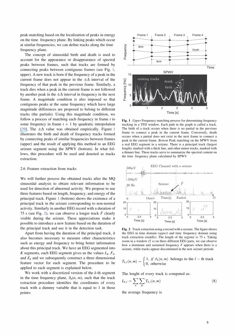
The concept of sinusoidal birth and death is used to

account for the appearance or disappearance of spectral

peaks between frames, such that tracks are formed by

connecting peaks between contiguous frames (see Fig. 1,

upper). A new track is born if the frequency of a peak in the

current frame does not appear in the ±D interval of the

frequency of that peak in the previous frame. Similarly, a

track dies when a peak in the current frame is not followed

by another peak in the ±D interval in frequency in the next

frame. A magnitude condition is also imposed so that

contiguous peaks at the same frequency which have large

magnitude differences are proposed to belong to different

tracks (the partials). Using this magnitude condition, we

follow a process of matching each frequency in frame t to

some frequency in frame t ? 1 by quadratic interpolation

[39]. The ±D value was obtained empirically. Figure 1

illustrates the birth and death of frequency tracks formed

by connecting peaks of similar frequencies between frames

(upper) and the result of applying this method to an EEG

seizure segment using the SPWV (bottom). In what fol-

lows, this procedure will be used and denoted as tracks

extraction.

2.6 Feature extraction from tracks

We will further process the obtained tracks after the MQ

sinusoidal analysis to obtain relevant information to be

used for detection of abnormal activity. We propose to use

three features based on length, frequency, and energy of the

principal track. Figure 1 (bottom) shows the existence of a

principal track in the seizure corresponding to non-normal

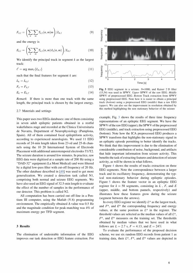
activity. Similarly in another EEG record with a duration of

75 s (see Fig. 2), we can observe a longer track F clearly

visible during the seizure. These appreciations make it

possible to introduce a new feature based on the duration of

the principal track and use it in the detection task.

Apart from having the duration of the principal track, it

also becomes necessary to measure other characteristics

such as energy and frequency to bring better information

about this principal track. We have an EEG segmented into

K segments, each EEG segment gives us the values Lk, Fk,

and Ek and we subsequently construct a three dimensional

feature vector for each segment. The procedure to be

applied to each segment is explained below.

We work with a discretized version of the k-th segment

in the time frequency plane, 0k(n, m), such that the track

extraction procedure identifies the coordinates of every

track with a dummy variable that is equal to 1 in those

points:

Tk;‘ðn;mÞ ¼ 1; if #kðn;mÞ belongs to the ‘� th track

0; otherwise

�

The lenght of every track is computed as:

Lk;‘ ¼Xn

Xm

Tk;‘ðn;mÞ ð8Þ

the average frequency is

Death

Birth

Birth

Fre

quen

cy

Time

Frame 1 Frame 2 Frame 3 Frame 4

Time [s]

Fre

quen

cy [H

z]

SPWV

1 2 3 4 50

5

10

15

Fig. 1 Upper Frequency matching process for determining frequency

tracking in a TFD window. Each path in the graph is called a track.

The birth of a track occurs when there is no partial in the previous

frame to connect a peak in the current frame. Conversely, death

occurs when a partial does not exist in the next frame to connect a

peak in the current frame. Bottom Peak matching on the SPWV from

a real EEG segment in a seizure. There is a principal track (largest

length), marked with a thick line, and other minor tracks, marked with

a thinner line. These tracks serve to summarize the spectral content on

the time frequency plane calculated by SPWV

0 2.5 50

10

20

Time [s]0 2.5 5

0

10

20

Time [s]

0 2.5 50

10

20

Time [s]

Fig. 2 Track extraction using a record with a seizure. The figure shows

the EEG in time domain (upper) and time frequency domain using

track extraction (middle). The length of the register is 75 s. Taking

zoom in a window (5 s) on three different EEG parts, we can observe

how a dominant and sustained frequency F appears when there is a

seizure, while tracks appear discontinued in the non seizure periods

Med Biol Eng Comput (2010) 48:321 330 325

13

5

Fk;‘ ¼Xn

Xm

Tk;‘ðn;mÞm !

=Lk;‘ ð9Þ

and the energy is

Ek;‘ ¼Xn

Xm

Tk;‘ðn;mÞ#kðn;mÞ !

=Lk;‘ ð10Þ

We identify the principal track in segment k as the largest

track:

‘0 ¼ arg max‘fLk;‘g ð11Þsuch that the final features for segment k are:

Lk ¼ Lk;‘0 ð12ÞFk ¼ Fk;‘0 ð13ÞEk ¼ Ek;‘0 ð14ÞRemark If there is more than one track with the same

length, the principal track is chosen by the largest energy.

2.7 Materials and settings

This paper uses two EEGs databases: one of them consisting

in seven adult epileptic patients obtained in a restful

wakefulness stage and recorded at the Clinica Universitaria

de Navarra, Department of Neurophysiology (Pamplona,

Spain). All of them contained focal epileptiform activity,

according to experienced neurologists. We used 11 EEG

records of 24-min length taken from 23-rd and 25-th chan-

nels using the 10 20 International System of Electrode

Placement with additional anterotemporal electrodes T1/T2.

The seizure duration is around few minutes. In practice, raw

EEG data were digitized at a sample rate of 200 Hz using a

‘‘DAD-32’’ equipment (La Mont Medical) and were filtered

by a digital low-pass filter with cut-off frequency of 20 Hz.

The other database described in [49] was used to get more

generalization. We created a detection task called N1,

comprising both normal and seizure EEG segments. We

have also used an EEG signal of 32.5-min length to evaluate

the effect of the number of samples in the performance of

our detector. This problem is called N2.

All computation has been carried out off-line in a Pen-

tium III computer, using the Matlab (V.6) programming

environment. The empirically obtained D value was 0.5 Hz

and the magnitude condition for peak-matching was 4% of

maximum energy per TFD segment.

3 Results

The elimination of undesirable information of the EEG

improves our task detection or EEG feature extraction. For

example, Fig. 3 shows the results of three time frequency

representations of an epileptic EEG segment. We have the

SPWVof the rawEEG(upper), theSPWVof the preprocessed

EEG (middle), and track extraction using preprocessed EEG

(bottom). Note how the ICA preprocessed EEG produces a

SPWV transform that highlights the non-stationary signal in

an epileptic episode permitting to better identify the tracks.

We think that this improvement is due to the elimination of

considerable contribution of noise, background, and artifacts

that hide important information from seizure activity. This

benefits the task of extracting features and detection of seizure

activity, as will be shown in what follows.

Figure 4 shows the results of tracks extraction on three

EEG segments. Note the correspondence between a larger

track and its oscillatory frequency, demonstrating the typ-

ical non-stationary behavior during epileptic episodes.

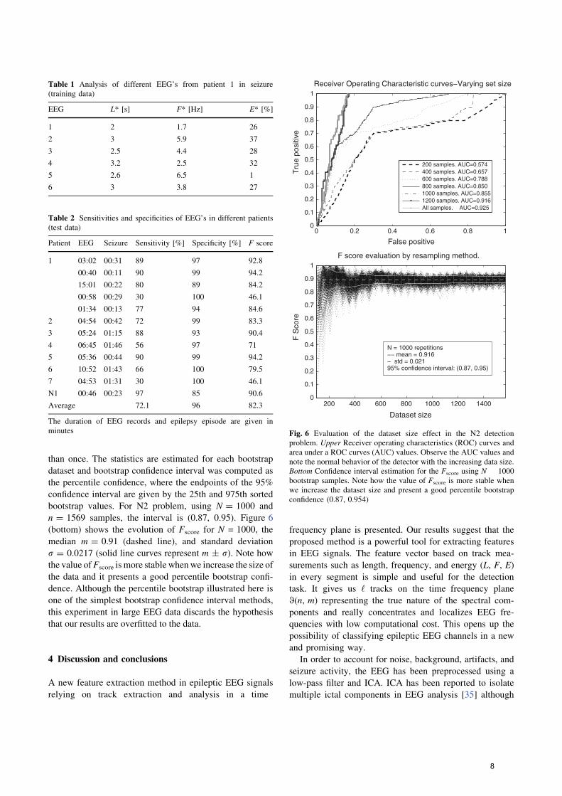
Figure 5 shows the feature vector in an epileptic EEG

register for k = 58 segments, consisting in L , F, and E

(upper, middle, and bottom pannels, respectively) and

illustrates how these features grow during the seizure

(segment between the arrows).

In every EEG register we identify L* as the largest track,

and F*, and E* the corresponding frequency and energy

values, at the same position as L* in the register. The

threshold values are selected as the median values of all L*,

F*, and E* measures on the training set. The thresholds

obtained by median values that we have used in what

follows are L ¼ 2:7 s, F ¼ 4:13, and E ¼ 24%

To evaluate the performance of the proposed decision

scheme, we use six random EEG records from patient 1 as

training data, their L*, F*, and E* values are depicted in

freq

uenc

y

0

5

10

0 1 2 3 4 50

5

10

Time [s]

freq

uenc

y

0

5

10

freq

uenc

y

Fig. 3 EEG segment in a seizure. N=1000, and Kaiser 2 D filter

(15,54) was used in SPWV. Upper SPWV of the raw EEG. MiddleSPWV of preprocessed EEG. Bottom Track extraction from SPWV

using preprocessed EEG. Note how it is easier to obtain a principal

track (bottom) using a preprocessed EEG (middle) than a raw EEG

(upper). We can also see the improvement in resolution obtained by

this method highlighting the non stationary behavior of the seizure

326 Med Biol Eng Comput (2010) 48:321 330

13

6

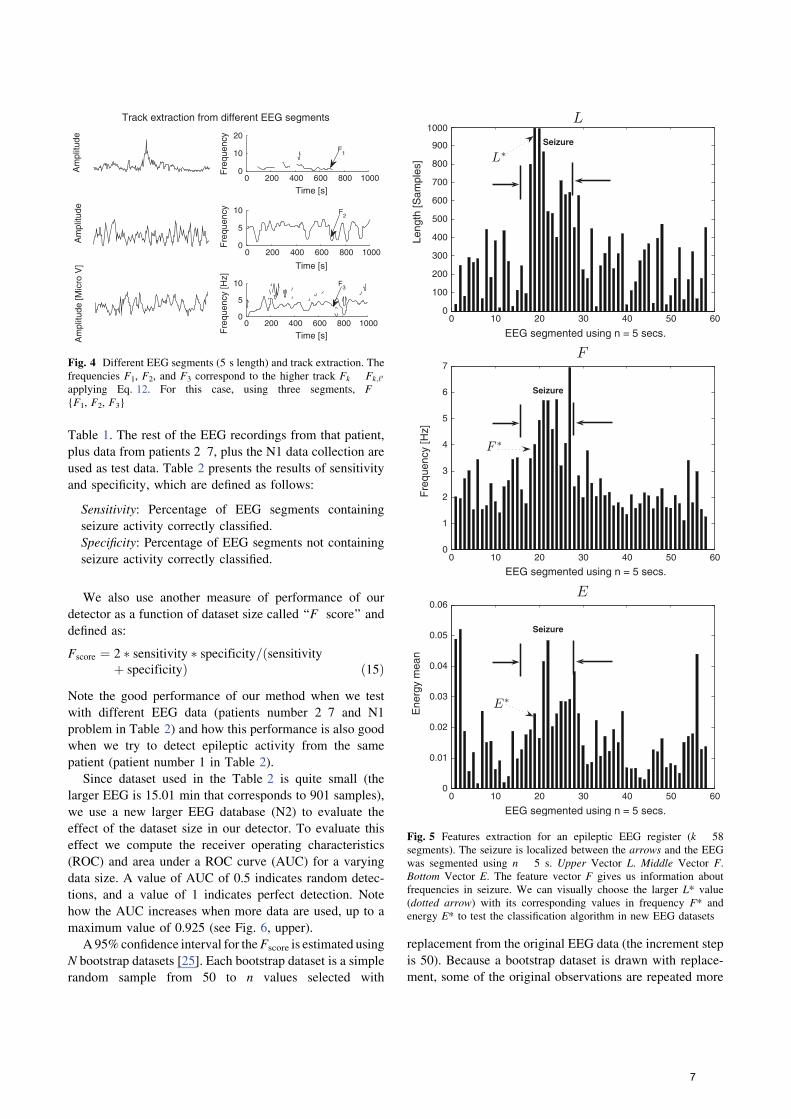
Table 1. The rest of the EEG recordings from that patient,

plus data from patients 2 7, plus the N1 data collection are

used as test data. Table 2 presents the results of sensitivity

and specificity, which are defined as follows:

Sensitivity: Percentage of EEG segments containing

seizure activity correctly classified.

Specificity: Percentage of EEG segments not containing

seizure activity correctly classified.

We also use another measure of performance of our

detector as a function of dataset size called ‘‘F score’’ and

defined as:

Fscore ¼ 2 � sensitivity � specificity=ðsensitivityþ specificityÞ ð15Þ

Note the good performance of our method when we test

with different EEG data (patients number 2 7 and N1

problem in Table 2) and how this performance is also good

when we try to detect epileptic activity from the same

patient (patient number 1 in Table 2).

Since dataset used in the Table 2 is quite small (the

larger EEG is 15.01 min that corresponds to 901 samples),

we use a new larger EEG database (N2) to evaluate the

effect of the dataset size in our detector. To evaluate this

effect we compute the receiver operating characteristics

(ROC) and area under a ROC curve (AUC) for a varying

data size. A value of AUC of 0.5 indicates random detec-

tions, and a value of 1 indicates perfect detection. Note

how the AUC increases when more data are used, up to a

maximum value of 0.925 (see Fig. 6, upper).

A 95% confidence interval for theFscore is estimated using

N bootstrap datasets [25]. Each bootstrap dataset is a simple

random sample from 50 to n values selected with

replacement from the original EEG data (the increment step

is 50). Because a bootstrap dataset is drawn with replace-

ment, some of the original observations are repeated more

0 200 400 600 800 10000

5

10

Time [s]Fre

quen

cy [H

z]

0 200 400 600 800 10000

5

10

Time [s]

Fre

quen

cy

0 200 400 600 800 10000

10

20

Time [s]

Fre

quen

cy

Am

plitu

de [M

icro

V]

Am

plitu

deA

mpl

itude

F1

F2

F3

Track extraction from different EEG segments

Fig. 4 Different EEG segments (5 s length) and track extraction. The

frequencies F1, F2, and F3 correspond to the higher track Fk Fk;‘0

applying Eq. 12. For this case, using three segments, F{F1, F2, F3}

0 10 20 30 40 50 600

100

200

300

400

500

600

700

800

900

1000

EEG segmented using n = 5 secs.

Leng

th [S

ampl

es]

Seizure

0 10 20 30 40 50 600

1

2

3

4

5

6

7

EEG segmented using n = 5 secs.

Fre

quen

cy [H

z]

Seizure

0 10 20 30 40 50 600

0.01

0.02

0.03

0.04

0.05

0.06

EEG segmented using n = 5 secs.

Ene

rgy

mea

n

Seizure

Fig. 5 Features extraction for an epileptic EEG register (k 58

segments). The seizure is localized between the arrows and the EEG

was segmented using n 5 s. Upper Vector L. Middle Vector F.Bottom Vector E. The feature vector F gives us information about

frequencies in seizure. We can visually choose the larger L* value

(dotted arrow) with its corresponding values in frequency F* and

energy E* to test the classification algorithm in new EEG datasets

Med Biol Eng Comput (2010) 48:321 330 327

13

7

than once. The statistics are estimated for each bootstrap

dataset and bootstrap confidence interval was computed as

the percentile confidence, where the endpoints of the 95%

confidence interval are given by the 25th and 975th sorted

bootstrap values. For N2 problem, using N = 1000 and

n = 1569 samples, the interval is (0.87, 0.95). Figure 6

(bottom) shows the evolution of Fscore for N = 1000, the

median m = 0.91 (dashed line), and standard deviation

r = 0.0217 (solid line curves represent m ± r). Note howthe value ofFscore is more stable whenwe increase the size of

the data and it presents a good percentile bootstrap confi-

dence. Although the percentile bootstrap illustrated here is

one of the simplest bootstrap confidence interval methods,

this experiment in large EEG data discards the hypothesis

that our results are overfitted to the data.

4 Discussion and conclusions

A new feature extraction method in epileptic EEG signals

relying on track extraction and analysis in a time

frequency plane is presented. Our results suggest that the

proposed method is a powerful tool for extracting features

in EEG signals. The feature vector based on track mea-

surements such as length, frequency, and energy (L, F, E)

in every segment is simple and useful for the detection

task. It gives us ‘ tracks on the time frequency plane

0(n, m) representing the true nature of the spectral com-

ponents and really concentrates and localizes EEG fre-

quencies with low computational cost. This opens up the

possibility of classifying epileptic EEG channels in a new

and promising way.

In order to account for noise, background, artifacts, and

seizure activity, the EEG has been preprocessed using a

low-pass filter and ICA. ICA has been reported to isolate

multiple ictal components in EEG analysis [35] although

Table 1 Analysis of different EEG’s from patient 1 in seizure

(training data)

EEG L* [s] F* [Hz] E* [%]

1 2 1.7 26

2 3 5.9 37

3 2.5 4.4 28

4 3.2 2.5 32

5 2.6 6.5 1

6 3 3.8 27

Table 2 Sensitivities and specificities of EEG’s in different patients

(test data)

Patient EEG Seizure Sensitivity [%] Specificity [%] F score

1 03:02 00:31 89 97 92.8

00:40 00:11 90 99 94.2

15:01 00:22 80 89 84.2

00:58 00:29 30 100 46.1

01:34 00:13 77 94 84.6

2 04:54 00:42 72 99 83.3

3 05:24 01:15 88 93 90.4

4 06:45 01:46 56 97 71

5 05:36 00:44 90 99 94.2

6 10:52 01:43 66 100 79.5

7 04:53 01:31 30 100 46.1

N1 00:46 00:23 97 85 90.6

Average 72.1 96 82.3

The duration of EEG records and epilepsy episode are given in

minutes

0 0.2 0.4 0.6 0.8 10

0.1

0.2

0.3

0.4

0.5

0.6

0.7

0.8

0.9

1

False positive

Tru

e po

sitiv

e

Receiver Operating Characteristic curves−Varying set size

200 samples. AUC=0.574400 samples. AUC=0.657600 samples. AUC=0.788800 samples. AUC=0.8501000 samples. AUC=0.8551200 samples. AUC=0.916All samples. AUC=0.925

200 400 600 800 1000 1200 14000

0.1

0.2

0.3

0.4

0.5

0.6

0.7

0.8

0.9

1F score evaluation by resampling method.

Dataset size

F S

core

N = 1000 repetitions−− mean = 0.916− std = 0.02195% confidence interval: (0.87, 0.95)

Fig. 6 Evaluation of the dataset size effect in the N2 detection

problem. Upper Receiver operating characteristics (ROC) curves and

area under a ROC curves (AUC) values. Observe the AUC values and

note the normal behavior of the detector with the increasing data size.

Bottom Confidence interval estimation for the Fscore using N 1000

bootstrap samples. Note how the value of Fscore is more stable when

we increase the dataset size and present a good percentile bootstrap

confidence (0.87, 0.954)

328 Med Biol Eng Comput (2010) 48:321 330

13

8

there is a noticeable difference between ICA and low-pass

filter when a visual inspection of the time frequencies

plane is done. Automatic EOG removal has proved to be

useful except when EEG is very contaminated with muscle

artifacts because ICA is not able to eliminate them totally.

Muscle artifacts are more difficult to suppress since its

morphology and topography causes a confusion with the

abnormal spikes. We think that this problem does not

considerably affect the performance of the detection task

because the seizure information is not affected if we do not

eliminate the muscle artifacts. Additionally, a low-pass

filter was chosen because it is possible to detect epileptic

activity on low frequencies and the EEG typically has a

frequency content from 1 to 40 Hz [37].

We have seen the presence of tracks on the time fre-

quency plane during seizure events as also observed by

other authors [11, 50]. In [11, 9, 10] the authors found a

time frequency seizure criteria based on two calibrations

in time and time frequency domain. In our case, we have

proposed a new form of extracting features based on

principal track by following the ridges (tracks) on the time

frequency plane and obtaining measures such as duration,

frequency, and energy. The length of the ridge of the main

time frequency EEG component has been previously pro-

posed in a number of applications including EEG [9, 10,

43]. Features such as energy and other frequency-based

features have been widely used in the literature dealing

with EEG. The extraction method proposed here is much

simpler than others previously proposed in the literature,

since they need many calibrations to properly work.

Another important issue is the applicability of the

method to any distribution due to its non-dependency to a

particular TFD. For example, the Ridges Extraction

method [5], which is a good approach for the reassignment

method [23], is able to extract relevant information from

the time frequency plane, but it depends on the values

obtained by reassignment method affecting the time com-

putation [23]. This problem is presented in [13] when the

frequency update is not easy because it is necessary to

modify the ridge detection algorithm.

The proposed technique could also be used in any sce-

nario where different types of EEG activity have to be

detected and associated to particular events. In brain

computer interface (BCI) applications, the model could be

adopted to detect ‘‘brain actions’’, e.g., moving up, left,

right or down a cursor on a screen using EEG readings. The

detection of other brain disorders could also be tackled [28,

46, 1]. However, further research is needed to validate the

discriminative capability of the track extraction features in

these new scenarios. Since the algorithm takes information

from a TFD, it is necessary a suitable distribution for EEG

signals, subject to the following compromise: high-quality

resolution, good detection, and low computation time [8].

With a good TFD choice, the localizations of both ampli-

tude and frequency peaks are less problematic. We have

chosen the smooth pseudo Wigner-Ville (SPWV) as the

TFD suitable for EEG signal detection as it provides good

resolution, low cross-terms, and is computationally effi-

cient [23].

Although the detector presented a good performance by

the evaluation of receiver operating (ROC) curves,

‘‘F score’’ measure and confidence intervals, another

important issue is how to select the threshold to yield high

sensitivity. The particular value of magnitude threshold and

D used during track extraction algorithm do not appreciably

affect the results, but a good choice in these values is

required. Likewise, it is necessary a long-term analysis to

understand the epilepsy behavior and to account for all

possible L values (maximum and minimum) in seizure,

because our EEG data records were not very large. Further

research into this matter including how to incorporate a

threshold selection into an automatic seizure algorithm is

worthwhile. Future works implies the study of a wide range

of machine learning methods to better exploit the features

proposed here to finally obtain improved seizure detections.

In conclusion, this paper presents a new EEG feature

vector based on track measurements such as length, fre-

quency, and energy (L, F, E) using the time frequency

distributions (TFD) and MQ sinusoidal analysis. The per-

formance during detection shows that our feature vector is

a suitable approach for epileptic seizure detection, it gen-

eralizes well, and opens the possibility of using this method

in other scenarios such as brain computer interface (BCI)

and detection of other brain disorders.

Acknowledgments This work has been funded by the Spain CICYT

grant TEC2008 02473.

References

1. Abasolo D, Escudero J, Hornero R, Gomez C, Espino P (2008)

Approximate entropy and auto mutual information analysis of the

electroencephalogram in Alzheimer’s disease patients. Med Biol

Eng Comput 46:1019 1028

2. Acir N, Oztura I, Kuntalp M, Baklan B, Guzelis C (2005)

Automatic detection of epileptiform events in EEG by three stage

procedure based on artificial neural networks. IEEE Trans Bio

med Eng 52:30 40

3. Afonso VX, Tompkins WJ (1995) Detecting ventricular fibrilla

tion. IEEE Eng Med Biol 14:152 159

4. Akay M (1996) Detection and estimation methods for biomedical

signals. Academic Press, New Jersey

5. Auger F, Aldrin P, Goncalves P, Lemoine O (1996) Time fre

quency toolbox for Matlab, user’s guide and reference guide.

CNRS (France) and Rice University (USA), Paris

6. Barlow JS (1985) Methods of analysis of nonstationary EEGs,

with emphasis on segmentation techniques: a comparative

review. J Clin Neurophysiol 2:267 304

Med Biol Eng Comput (2010) 48:321 330 329

13

9

7. Blume WT, Young GB, Lemieux JF (1984) EEG morphology of

partial epileptic seizures. Electroencephalogr Clin Neurophysiol

4:295 302

8. Boashash B (2003) Time frequency signal analysis and process

ing. A comprehensive reference. Elsevier, Oxford

9. Boashash B, Mesbah M (2001) A time frequency approach for

newborn seizure detection. IEEE Eng Med Biol Mag 20(5):54 64

10. Boashash B, Mesbah M (2002) Time frequency methodology for

newborn electroencephalographic seizure detection. In: Papand

reou Suppappola A (ed) Applications in time frequency signal

processing. CRC Press, Boca Raton, Florida

11. Boashash B, Carson H, Mesbah M (2000) Detection of seizures in

newborns using time frequency of EEG signals. Proceedings of

Tenth IEEE workshop on statistical signal and array processing,

pp 564 568

12. Cardoso JF (1998) Blind signal separation: statistical principles.

Proc IEEE 86:2009 2025

13. Carmona RA, Hwang WL, Torresani B (1999) Multiridge

detection and time frequency reconstruction. IEEE Trans Signal

Process 47:480 492

15. Cohen L (1989) Time frequency distributions a review. Proc

IEE 77:941 981

14. Cohen L (1995) Time frequency analysis. Prentice Hall, Upper

Saddle River, NJ

16. Colder BW, Frysinger RC, Wilson CL, Harper RM, et al (1996)

Decreased neuronal burst discharge near site of seizure onset in

epileptic human temporal lobes. Epilepsia 37:113 121

17. Durka PJ (1996) Time frequency analysis of EEG. Thesis

Institute of Experimental Physics, Warsaw University

18. Freeman WJ (1963) The electrical activity of a primary sensory

cortex: analysis of EEG waves. Int Rev Neurobiol 5:53 119

19. Gonzalez B, Sanei S, Chambers JA (2003) Support vector

machines for seizure detection. Proceedings of the IEEE ISSPIT,

pp 126 129

21. Gotman J (1982) Automatic recognition of epileptic seizures in

the EEG. Electroencephalogr Clin Neurophysiol 54:530 540

20. Gotman J (1983) Measurement of small time differences between

EEG channels: methods and application to epileptic seizure

propagation. Electroencephalogr Clin Neurophysiol 56:501 514

22. Grewal S, Gotman J (2005) An automatic warning system for

epileptic seizures recorded on intracerebral EEGs. Clin Neuro

physiol 116:2460 2472

23. Guerrero C, Malanda A, Iriarte J (2005) Time frequency EEG

analysis in epilepsy: what is more suitable? Proceedings of the

IEEE ISSPIT, pp 202 207

24. Guerrero Mosquera C, Navia Vazquez A (2009) Automatic

removal of ocular artifacts from EEG data using adaptive filtering

and independent component analysis. Proceedings of the 17th

European signal processing conference (EUSIPCO), pp 2317

2321

25. Harrell FE (2001) Regression modeling strategies. Springer, New

York

26. Hassanpour H, Mesbah M, Boashash B (2004) Time frequency

feature extraction of newborn EEG seizure using SVD based

techniques. Proceedings of EURASIP. J Appl Signal Process

16:2544 2554

27. He P, Wilson G, Russel C (2004) Removal of ocular artifacts

from electro encephalogram by adaptive filtering. Med Biol Eng

Comput 42:407 412

28. Hinrikus H, Suhhova A, Bachmann M, et al (2009) Electroen

cephalographic spectral asymmetry index for detection of

depression. Med Biol Eng Comput 47:1291 1299

29. Hlawatsch F, Boudreaux Bartels GF (1992) Linear and quadratic

time frequency signal representation. IEEE SP Mag 9:21 67

30. Hoeve M, Zwaag BJ, Slump K, Jones R (2003) Detecting epi

leptic seizure activity in the EEG by independent component

analysis. Proceedings of the ProRISC workshop on circuits sys

tems and signal processing, pp 373 378

31. Iriarte J, Urrestarazu E, Valencia M, Alegre M, Malanda A, Viteri

C, Artieda J (2003) Independent component analysis as a tool to

eliminate artifacts in EEG: a quantitative study. J Clin Neuro

physiol 20:249 257

32. Joyce CA, Gorodnitsky IF, Kutas M (2004) Automatic removal

of eye movement and blink artifacts from EEG data using blind

component separation. Psychophysiology 41:1 13

33. Kay SM, Marple SL (1981) Spectrum analysis: a modern per

spective. Proc IEEE 69:1380 1419

34. Lehnertz K, Elger CE (1995) Spatio temporal dynamics of the

primary epileptogenic area in temporal lobe epilepsy character

ized by neuronal complexity loss. Electroencephalogr Clin Neu

rophysiol 95:108 117

35. Le Van P, Urrestarazu E, Gotman J (2006) A system for auto

matic removal in ictal scalp EEG based on independent compo

nent analysis and Bayesian classification. Clin Neurophysiol

117:912 927

36. Li H, Sun Y (2005) The study and test of ICA algorithms. Proc

IEEE Wirel Commun Netw Mob Comput 1:602 605

37. Lin Z Y, Chen JDZ (1996) Advances in time frequency analysis

of biomedical signals. Crit Rev Biomed Eng 24:1 70

38. Makeig S, Bell AJ, Jung TP, Sejnowski T (1996) Independent

component analysis of electroencephalogram data. Adv Neural

Inf Process Syst 145 151

39. McAulay RJ, Quatieri TF (1986) Speech analysis/synthesis based

on a sinusoidal representation. IEEE Trans Acoust Speech Signal

Process 34:744 754

40. Mohseni HR, Maghsoudi A, Shamsollahi MB (2006) Seizure

detection in EEG signals: a comparision of different approaches.

Proceedings of the 28th IEEE annual EMBS international con

ference, pp 6724 6727

41. Muthuswamy J, Thakor NV (1998) Spectral analysis methods for

neurological signals. J Clin Neurophysiol 83:1 14

42. Osorio I, Frei MG, Wilkinson SB (1998) Real time automated

detection and quantitative analysis of seizures and short term

prediction of clinical onset. Epilepsy 39:615 627

43. Rankine R, Mesbah M, Boashash B (2007) IF estimation for

multicomponent signals using image processing techniques in the

time frequency domain. Signal Process 87:1234 1250

44. Sclabassi RJ, Sun M, Krieger DN, Scher MS (1990) Time fre

quency analysis of the EEG signal. Proceedings of the interna

tional conference on signal processing, pp 935 938

45. Senhadji L, Wendling F (2002) Epileptic transient detection:

wavelets and time frequency approaches. Neurophysiol Clin

32:175 192

46. Swarnkar V, Abeyratne UR, Hukins C, Duce B (2009) A state

transition based method for quantifying EEG sleep fragmenta

tion. Med Biol Eng Comput 47:1053 1061

47. Tognola G, Ravazzani P, Minicucci F, Locatelli T, et al (1996)Analysis of temporal non stationarities in EEG signals by means

of parametric modelling. Technol Health Care 4:169 185

48. Tseng SY, Chen RC, Chong FC, Kuo TS (1995) Evaluation of

parametric methods in EEG signal analysis. Med Eng Phys

17:71 78

49. Tzallas AT, Tsipouras MG, Fotiadis DI (2007) The use of time

frequency distributions for epileptic seizure detection in EEG

recordings. Proceedings of the IEEE EMBS, pp 3 6

50. Williams WJ, Zavery HP, Sackellares JC (1995) Time frequency

analysis in electrophysiology signals in epilepsy. IEEE Eng Med

Biol 14:133 143

330 Med Biol Eng Comput (2010) 48:321 330

13

10