natural circulating flat plate collectors - uio - duo

UNIVERSITY OF OSLODepartment of Physics

Naturalcirculating flatplate collectorsInvestigations of a newmaterial andperformance simulations

Master’s thesis inPhysics, TeacherEducationProgramme

Aylin Maria Dursun

May 27th, 2013

Abstract

Solar energy can be utilized to heat water with the use of flat plate collectors.Effort is made to reduce the cost of solar water heating technology in order tomake it economically competitive to conventional energy. An absorber materialis tested on component level and performance related aspects are studied. Thematerial has a lower price than the polymer materials currently used in glazedcollectors, and therefore it has the potential to lower the cost of solar flat platecollectors. The performance related aspects are tested on a partially glazed, nat-ural circulating flat plate collector, referred to as the Duo-Collector. The aim ofletting the collector be partially glazed is to prevent the heat carrier from boiling.Samples cut from an extruded absorber sheet were exposed to 140 ◦C and 150 ◦Cfor different periods of time. These were used to map the mechanical properties ofthe material. The samples exposed to 150 ◦C were used to map dimensional andoptical changes. The results from the material-related studies on component levelshow that no failure occurs for any of the ageing periods which were realized inthe time frame of the present work. The extruded absorber sheet has a sufficientlyhigh absorptance and dimensional stability. These findings have strengthened thematerial’s position as a candidate for use in solar thermal applications. The per-formance of the Duo-Collector has been simulated with MATLAB R©. It is foundthat the system is suitable as a method for preventing the fluid in the collectorfrom boiling. The efficiency of such a system was also investigated. For low op-erating temperatures the efficiency of a Duo-Collector is approximately equal tothe efficiency of a fully glazed or an unglazed collector. The efficiency of all thecollectors decrease with increasing operating temperatures, and the efficiency ofthe Duo-Collector is between that of a fully glazed and that of an unglazed col-lector for all operating temperatures above approximately 10 ◦C. Under certaincircumstances the Duo-Collector can cool the water. This effect needs to be in-vestigated further. Since only steady-state conditions are studied in this work,further analysis must be performed to compare how the Duo-Collector performsfor different applications.

I

Acknowledgements

I am deeply grateful to Professor John Rekstad and Dr. Michaela Meir for givingme the opportunity to write this master´s thesis and for always being positive,flexible and supporting. It has been a great experience to work with you.

The last eighteen weeks have given me a large variety of challenges, and I amthankful to all the people who have made the process a little easier; thanks toall the friendly people at SAFE, thank you Dag for lending me a heating cabinet,thanks to the people doing IT support and to the guys at the workshop. Thankyou Professor John Grue for your interest and help when I showed up in your office.

Thank you for your friendship Inger Helene and Ida.

My lovely family has always been a great support. Thank you for your uncondi-tional love and your second opinion.

Aylin Dursun

III

Contents

1 Introduction 1

2 Solar heating systems 52.1 Studies on low cost systems . . . . . . . . . . . . . . . . . . . . . . 52.2 Flat plate collectors . . . . . . . . . . . . . . . . . . . . . . . . . . . 72.3 Thermosyphon systems . . . . . . . . . . . . . . . . . . . . . . . . . 92.4 Heat carrier temperature . . . . . . . . . . . . . . . . . . . . . . . . 102.5 The Duo-Collector . . . . . . . . . . . . . . . . . . . . . . . . . . . 11

3 Polymer science 153.1 Polypropylene . . . . . . . . . . . . . . . . . . . . . . . . . . . . . . 153.2 Elasticity and plasticity . . . . . . . . . . . . . . . . . . . . . . . . 153.3 Ageing . . . . . . . . . . . . . . . . . . . . . . . . . . . . . . . . . . 173.4 Mathematical model of degradation . . . . . . . . . . . . . . . . . . 183.5 Service life estimations . . . . . . . . . . . . . . . . . . . . . . . . . 19

4 Experimental setup 214.1 The alphameter . . . . . . . . . . . . . . . . . . . . . . . . . . . . . 214.2 The Instron 3345 machine . . . . . . . . . . . . . . . . . . . . . . . 214.3 Termaks heating cabinets . . . . . . . . . . . . . . . . . . . . . . . . 224.4 Absorber material and design . . . . . . . . . . . . . . . . . . . . . 22

5 Experimental studies 255.1 Approach . . . . . . . . . . . . . . . . . . . . . . . . . . . . . . . . 255.2 Results . . . . . . . . . . . . . . . . . . . . . . . . . . . . . . . . . . 30

6 Simulation 336.1 Approach . . . . . . . . . . . . . . . . . . . . . . . . . . . . . . . . 336.2 Results . . . . . . . . . . . . . . . . . . . . . . . . . . . . . . . . . . 40

V

VI CONTENTS

7 Discussion 457.1 Discussion of experimental results . . . . . . . . . . . . . . . . . . . 457.2 Discussion of results from simulation . . . . . . . . . . . . . . . . . 49

8 Summary 53

Bibliography 55

Appendices 59

A Results from earlier studies 61

B MATLAB scripts 65

C Indentation tests 69

D Raw data: dimensions 71

E Raw data: absorptance 73

CONTENTS VII

NomenclatureA collector area [m2]Ac cross section area [m2]b plate thickness [m]c specific heat capacity [J/(kgK)]C proportionality constantC1 constant of integrationD thermal doseDc critical thermal dosedx aperture between inner walls [m]dz aperture between plates [m]Ea activation energyF force needed to bring specimen to fracture pointF0 force needed to bring unexposed specimen to fracture pointFc critical loadF ′ collector efficiency factorg acceleration due to gravity [m/s2]G solar irradiance incident on collector surface [W/m2]h height of absorber [m]h1 height of glazed part of absorber [m]h2 height of unglazed part of absorber [m]H defined as kp/b [W/(m2K)]k the Boltzmann constantk1 loss coefficient to be fitted experimentally [W/m2K]k2 loss coefficient to be fitted experimentally [W/m2K2]kp thermal conductivity of plate [W/(mK)]m massn reaction orderP glazing fraction [%]P0 ambient pressure [Pa]P1 pressure at the bottom of water column [Pa]qu unit area useful energy rate [W/m2]Qu useful energy rate [W]S absorbed solar radiation [W/m2]t time [s]T temperature [◦C]Ta ambient temperature [◦C]Td temperature difference between heat carrier and ambientTf temperature of fluid/ heat carrier [◦C]Ti inlet temperature relative to ambient temperature [K]To outlet temperature relative to ambient temperature [K]Tp temperature of plate facing the sun [◦C]Ts stagnation temperature [◦C]T̄ mean value of heat carrier temperature [◦C]T ′ temperature at the border between glazed and unglazed region relative to ambient [K]Ub back loss coefficient [W/(m2K)]UL collector overall loss coefficient [W/(m2K)]Ut top loss coefficient [W/(m2K)]v magnitude of heat carrier velocity in the upstream region [m/s]V̇ volume flow rate [m3/s]

VIII CONTENTS

Greek letters

α absorptance of absorber materialη efficiencyη0 efficiency for T̄ = Taρ density [kg/m3]σm standard deviation of the meanτ transmittance of glazingχ reaction rate

Chapter 1

Introduction

There are strong indications that the effect of human activity since 1750 has ledto a net global warming, and that the use of fossile energy ressources must bereduced in order to prevent irreversible climate changes (IPCC, 2007). The con-sequences of global warming are worsening with increasing temperature change.Some of the regional impacts associated with global warming are increased waterstress, sea level rise and loss of biodiversity and food security. The world hasan increasing energy demand due to economical and population growth, and to-day’s energy supply is based primarily on fossil fuels, which are responsible forthe majority of greenhouse gas emission. The global warming can be reducedby reducing the emission of greenhouse gases and hence there is a need for devel-oping and improvement of methods for utilizing renewable resources (IPCC, 2007).

Energy from the sun can be converted to electricity with the use of solar cells orby concentrating solar power. In addition the radiant energy from the sun can beconverted to heat by the use of solar collectors. In a solar collector an absorberconverts radiation from the sun to heat, and the heat is transferred to a circu-lating heat carrier as it passes through the absorber. Heat contains less exergythan electricity, and can hence be regarded as energy with lower quality than elec-tricity. Approximately 40 percent of the end-user energy consumption in EU25 ismoderate temperature heat (Rekstad, 2007). This demand does not require highquality energy. Taking this into account there is a large potential for reducing theuse of fossile fuels for instance by reducing the use of electric water heaters and oilburners by utilizing the energy from the sun. The International Energy Agency[IEA] has calculated that the amount of energy savings that glazed and unglazedsolar collectors contributed with by the end of 2010 approximately corresponds to53 million tons of CO2 per year (Weiss & Mauthner, 2012). This is comparable toNorway’s annual emission of greenhouse gases (Statistisk Sentralbyrå, 2013). 55countries, with an installed capacity corresponding to more than 90 percent of the

1

2 CHAPTER 1. INTRODUCTION

0

100

200

300

400

500

600

Solar ThermalHeat

Wind Power GeothermalPower

Photovoltaic Solar ThermalPower

Ocean TidalPower

Pro

du

ced

En

ergy

in 2

01

1 [

TWh

] power

204.3

514.0

90.0 70.2

2.9 0.8

heat

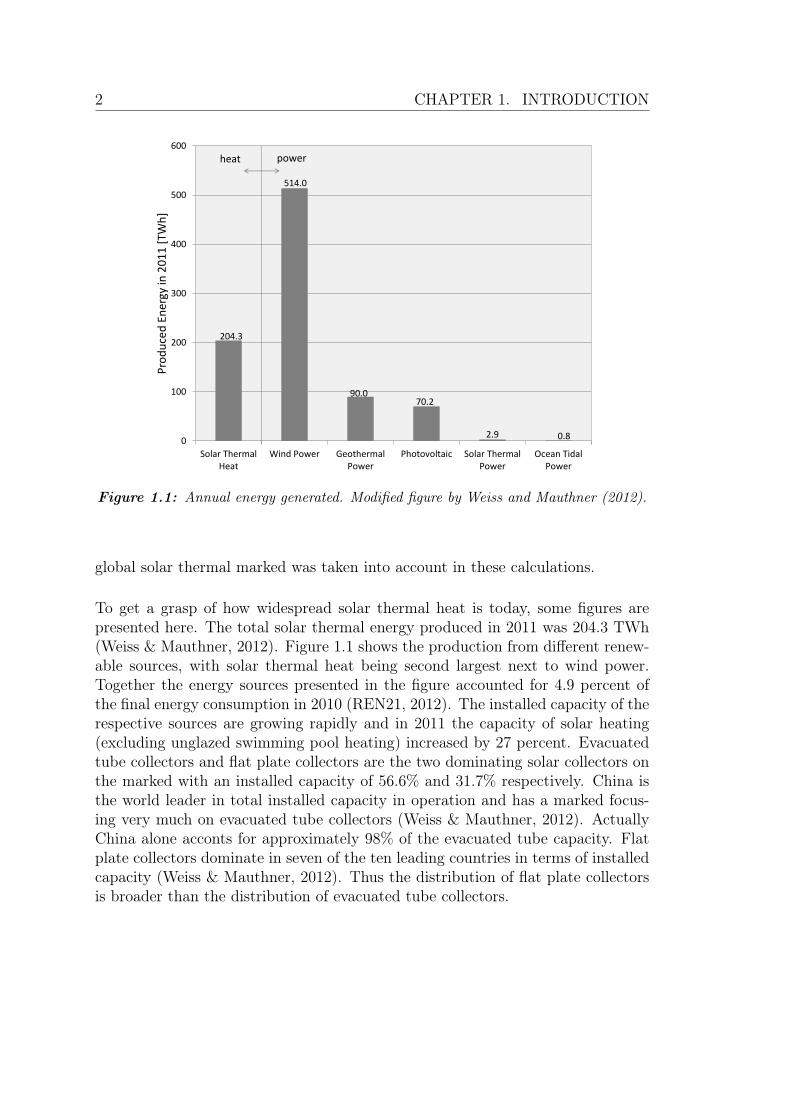
Figure 1.1: Annual energy generated. Modified figure by Weiss and Mauthner (2012).

global solar thermal marked was taken into account in these calculations.

To get a grasp of how widespread solar thermal heat is today, some figures arepresented here. The total solar thermal energy produced in 2011 was 204.3 TWh(Weiss & Mauthner, 2012). Figure 1.1 shows the production from different renew-able sources, with solar thermal heat being second largest next to wind power.Together the energy sources presented in the figure accounted for 4.9 percent ofthe final energy consumption in 2010 (REN21, 2012). The installed capacity of therespective sources are growing rapidly and in 2011 the capacity of solar heating(excluding unglazed swimming pool heating) increased by 27 percent. Evacuatedtube collectors and flat plate collectors are the two dominating solar collectors onthe marked with an installed capacity of 56.6% and 31.7% respectively. China isthe world leader in total installed capacity in operation and has a marked focus-ing very much on evacuated tube collectors (Weiss & Mauthner, 2012). ActuallyChina alone acconts for approximately 98% of the evacuated tube capacity. Flatplate collectors dominate in seven of the ten leading countries in terms of installedcapacity (Weiss & Mauthner, 2012). Thus the distribution of flat plate collectorsis broader than the distribution of evacuated tube collectors.

3

Solar collectors with high efficiency are on the marked today, but economicallythese have difficulties competing with conventional energy. According to Tsilingiris(2002, p. 137) the future of this technology depends on the development of “sim-ple, reliable and low cost systems, employing widely available recyclable materials”.The potential for cost reduction has motivated the development of solar collectorcomponents made of polymer materials.

The temperature in solar collectors may exceed the boiling temperature of theheat carrier. As boiling can damage the collector it must be avoided and this isnormally done by letting the heat carrier drain from the absorber and back intothe tank. Rekstad (2013) has proposed a new design which is thought to preventthe heat carrier from boiling. The new design is a natural circulating system witha passive heat control, referred to as the Duo-Collector.

Initially the plan was to investigate and estimate the service life of an absorbermaterial on component level. Due to the absence of quantitative results the aimof the work was expanded to include studies of performance related aspects of apartially glazed, natural circulating flat plate collector. The present work there-fore consists of two parts. The aim of the first part is to investigate an absorberproduced from a new material in order to determine if it is feasible for solar ther-mal applications. The material should sustain the thermal conditions in a solarcollector, have an absorptance which maintains good efficiencies and show gooddimensional stability in order to be feasible. The absorber is designed by Aventaand extruded by Kaysersberg Plastics from a polypropylene material produced byBorealis and is presented as a candidate for use in flat plate collectors.

Since the processing of the absorber sheets may affect the material, the tests areperformed on component level. Standard tests are not applicable on the givendesign, and therefore a test procedure developed at the University of Oslo andlater taken in use by others is used. The samples to be tested are extruded intoabsorber sheets and are tested for mechanical, dimensional and optical changes.The changes in the material’s properties during heat exposure are investigated fortwo different temperatures. Mechanical changes are mapped using an indentationtest investigated by Olivares (2008). The test procedure characterize the stabilityand strength of the internal structure as well as the surface of the tested specimens(Olivares, 2008).

The aim of the second part is to develop a simulation program and use it topredict the maximum temperatures obtainable in a Duo-Collector and investigatethe performance of such a system. The efficiency, flow velocity and temperature

4 CHAPTER 1. INTRODUCTION

increase of the heat carrier is calculated for different operating conditions.

Chapter 2

Solar heating systems

2.1 Studies on low cost systems

Effort is made to reduce the cost of solar water heating technology. According toAlghoul, Sulaiman, and Azmi (2005) polymers are pointed out as a promising al-ternative because they are cheap relative to metal, widely available, are lightweightand are tolerant to corrosion and freezing temperatures. A disadvantage of usingpolymers is their low thermal conductivity varying slightly around 0.2 W/(mK)(Tsilingiris, 1999). The design of the collector should seek to overcome this ob-stacle. According to Tsilingiris (2002) the most promising design is the extrudedparallel polymer plate absorber design, as it allows extended wetted surfaces ofthe absorber. In order to optimize the collector efficiency the thickness of the topplate should be minimized, but the plate has to be able to withstand hydrostaticloads and provide sufficient mechanical rigidity. With plate thickness smaller thantypically about 1 to 1.5 mm the collector efficiency factor will be higher than ap-proximately 0.96 (Tsilingiris, 1999). In a later paper Tsilingiris (2002) investigateda back absorbing parallel plate polymer absorber, where the top plate is transpar-ent, and the solar radiation is absorbed by the water stream and by the backplate. He developed a theoretical analysis for evaluation of the design. Comparedto a top absorbing design the author found that the instantaneous collector heatcollection efficiency increase in the order of 14%.

Flat plate collectors have been studied by many researchers and the theory is ex-tensively presented by Duffie and Beckman (2006). This theory is based on theassumption that temperature gradient through the absorber metal sheet is negli-gible. This does not apply to polymeric absorbers, and for the extruded parallelpolymer plate absorber design Tsilingiris (1999) performed an analysis and ad-justed the performance parameters.

5

6 CHAPTER 2. SOLAR HEATING SYSTEMS

Another design is studied by Chaurasia (2000). This collector consists of a networkof aluminum pipes embedded in concrete slabs, and are intended to cover build-ing roofs. These unglazed collectors are low-cost and have operating temperaturesvarying between 36 ◦C and 58 ◦C. An analysis and performance of another low-costsolar heater has been investigated by Siqueira, Vieira, and Damasceno (2011). Thesolar collector studied is a Low-Cost Solar Heater (LCSH) made entirely of poly-meric materials. It is composed of uncovered flat panels of rigid PVC. The articleauthors compare the efficiency of the collector with that of a conventional solarheater composed of a glass-covered copper collector and a stainless steel tank. Theresults indicated that the LCSH presented a good thermal performance in termsof heat loss as well as efficiency and temperature values attained. Although theLCSH is not as efficient as the conventional heater the authors recommends it asa good alternative for heating water. It is also concluded that there is a potentialfor significant economical savings when electric showers are replaced with a LCSH.

There has still not been done much research on the reliability, durability, and long-term performance of polymeric materials for solar collector applications (Alghoulet al., 2005). The research group at the University of Oslo has tested a varietyof polymer materials. The group has also developed and investigated a test pro-cedure for quantifying the mechanical degradation in absorber sheets caused byheat exposure (Olivares, 2008; da Silva, 2008). This test procedure has also beentaken into use by the Polymer Competence Center Leoben, Austria, the Instituteof Polymeric Materials and Testing at the Johannes Keppler University, Linz Aus-tria, Saudi Basic Industries Corporation (SABIC; former General Electric Plastics)and Fraunhofer Institute for Solar Energy Systems ISE, Germany (Meir, 2013).

An extruded triple-wall sheet made of a polyphenylene/polystyrene blend (PPE/PS)has been investigated by Olivares, Rekstad, Meir, Kahlen, and Wallner (2008,2010). In another study mechanical tensile tests were performed on thin filmsmade of different materials with a thickness of approximately 500 µm. The mate-rials tested were a polyphenylene ether polystyrene blend (PPE + PS), polycar-bonate (PC), two semi-crystalline polymers named polyamid 12 (PA12), two typesof crosslinked polyethylene (PE-X) and two types of polypropylene (PP) (Kahlen,Wallner, & Lang, 2010a, 2010b). Absorbers made of polyphenylene sulfide (PPS)have also been investigated (da Silva, 2008). Some of the results from these studiesare presented in Appendix A and will be compared to the results obtained in thepresent study. The polypropylene blend investigated in the present work has notbeen tested previously.

2.2. FLAT PLATE COLLECTORS 7

x

z y glazing

absorber insulation

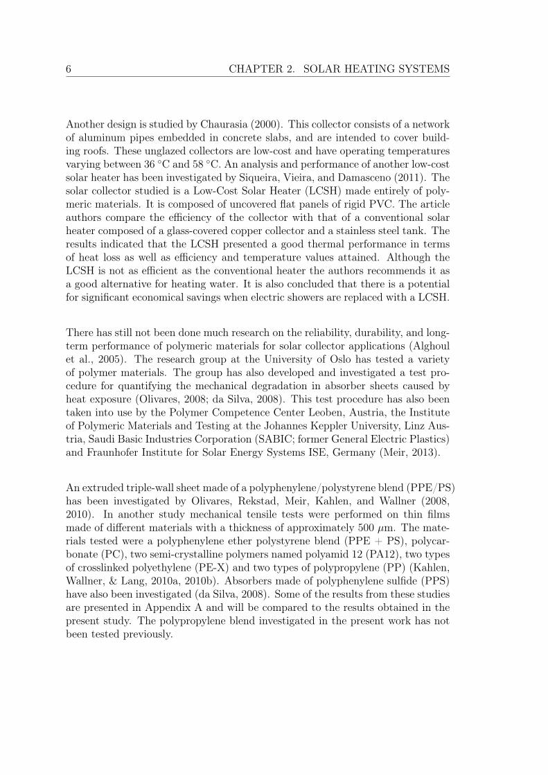
Figure 2.1: Schematic cross section of a flat plate collector.

2.2 Flat plate collectors

Description

The schematic diagram presented in Figure 2.1 illustrates the main parts of aglazed flat plate collector. The absorber sheet in the figure has an extruded par-allel polymer plate absorber design, which consists of two parallel polymer platesconnected with inner walls. The inner walls divide the space between the parallelplates into multiple channels. Solar radiation passes the glazing and is convertedto heat by the absorber. The heat carrier flows through the absorber channels,allowing heat to be transferred from the absorber to the fluid. The transpar-ent cover, or glazing, acts as a heat trap for infrared radiation (Alghoul et al.,2005). The glazing reduces convection and radiation losses from the absorber tothe surroundings, and the thermal insulation reduces conduction losses (Duffie &Beckman, 2006). It also protects the absorber from adverse weather conditions.(Alghoul et al., 2005).

Unit area heat rate

The heat rate at which energy is transferred from the sun to the heat carrier bothdepends on and changes the heat carrier temperature. In a region with uniformheat carrier temperature and during steady state conditions the unit area heatrate qu, measured in W/m2, is given by

qu = F ′[S − UL(Tf − Ta)], (2.1)

with

F ′ =1

1 + Ut/H,


and

UL = Ut

(1 +

1

1 + (H/Ub)

)+ Ub

(1 +

1

1− (H/Ub)

),

forH =

kpb.

In these equations UL is the overall heat loss coefficient, Tf is the heat carriertemperature, Ta is the ambient temperature, Ub and UT are heat loss coefficientsfor the base an top and b and kp are the thickness and the thermal conductivity ofthe plate respectively (Tsilingiris, 1999). S is the solar radiation absorbed by thecollector per unit area absorber. For a glazed absorber S can be approximated as

S ≈ Gατ1.01,

where G is the solar irradiance incident on the collector surface, α is the absorp-tance of the absorber sheet and τ is the transmittance of the glazing. The solarirradiance is measured in W/m2 and describes the rate of radiant solar energyincident on a surface per unit area (Duffie & Beckman, 2006). For an unglazedcollector S is given as

S = Gα

The expression in the square brackets in Eq. (2.1) represents the difference be-tween the absorbed solar radiation and the thermal energy loss due to conduction,convection and infrared radiation (Duffie & Beckman, 2006). During operation thetemperature of the heat carrier in the absorber will vary with location, implyingthat the unit area heat rate qu will vary with location.

Collector Efficiency

The efficiency η is a measure of the performance of the collector. It is definedas the ratio between the total useful gain delivered to the heat carrier during aspecified period of time and the solar energy incident on the collector during thesame period of time and is given by

η =Total useful gain

Solar energy received=

∫Qu dt

A

∫G dt

. (2.2)

In the literature the useful energy gain usually shows a first or second order depen-dency on the temperature difference between the mean heat carrier temperature

2.3. THERMOSYPHON SYSTEMS 9

and the ambient temperature (Morrison, 2001; Duffie & Beckman, 2006). Assum-ing stationary conditions a second order expression for the efficiency is approxi-mated by (Morrison, 2001):

η = η0 −k1(T̄ − Ta)

G− k2(T̄ − Ta)2

G, (2.3)

where η0, k1 and k2 are constants which can be fitted experimentally and T̄ is themean heat carrier temperature.

2.3 Thermosyphon systems

Description

Solar collectors can be active or passive. The passive systems are also referred toas thermosyphon systems (Duffie & Beckman, 2006). In contrast to active solarsystems, thermosyphon systems do not use mechanical devices, such as for in-stance electrical pumps or fans, to collect and transfer heat. Approximately threequarters of installed solar collector systems are thermosyphon systems (Weiss &Mauthner, 2012). The design shown in Figure 2.3 is a thermosyphon system.These systems use natural convection as the driving force for the circulation ofwater. The density of water decreases as the temperature rises, which causes thewater in the collector to rise into the tank as it is heated. As the circulation is gov-erned by temperature gradients in the tank, the circulation flow rate is naturallyin phase with the radiation level (Morrison, 2001). Under hard-water conditionsa common problem is scaling. Scaling occurs on polymer materials in about thesame rate as on copper and in a thermosyphon system it will reduce the flow ratedue to increased hydraulic resistance (Duffie & Beckman, 2006).

Volume flow rate

The volume flow rate V̇ is a measure of the rate at which the heat carrier flowsthrough the collector array. It is defined as the volume of heat carrier which passesthrough the system per unit time. In an active system this can be regulated byadjusting the pump. The amount of temperature increase through the collectorvaries with the flow rate. A low flow rate results in a larger temperature increasethrough the collector because the time it takes the heat carrier to pass throughthe collector is increased. If the flow rate is sufficiently low, stratification of thetemperature in the tank will occur. Cold water from the bottom of the tank willfeed the collector and the heated water will enter the top of the tank and stay


there. Stratification is important because this reduces the inlet temperature tothe collector leading to a higher collector efficiency (Rekstad & Meir, 2012). Also,the temperature in the top of the tank will be higher when the temperature distri-bution is stratified, leading to hotter tap water. In a system with a high volumeflow rate the water in the tank will have a homogeneous temperature distribution.The maximum temperature will hence be lower, but on the other hand the heatedvolume will be larger, allowing delivery of heated water for a longer time period.

The temperature rise through natural-convection systems has been observed tobe constant under a wide range of conditions. For well designed systems withoutserious flow restrictions the increase is observed to be approximately 10 ◦C (Duffie& Beckman, 2006). In a thermosyphon system the circulation is due to densitydifferences of the heat carrier in the system. The flow rate is governed by theuseful gain of the collector which produces temperature differences leading to thedensity differences (Duffie & Beckman, 2006). Modelling a specific system requiresiterative calculations because the temperatures and flow rates are interdependent(Duffie & Beckman, 2006).

The volume flow rate V̇ is given by

V̇ =dV

dt= Av,

The pressure P1 at the bottom of a water column with height h is given by

P1 = P0 +mg

Ac,

where P0 is the pressure at the top of the column, m is the mass of the watercolumn, g is the gravitational constant and A is the cross section area of thecolumn. In a column of constant temperature the density is constant and pressureis given by

P1 = P0 + ρgh. (2.4)

2.4 Heat carrier temperature

A flat plate collector exposed to a constant amount of solar irradiance and a con-stant ambient temperature for a sufficient amount of time will reach equilibrium.During equilibrium the amount of energy absorbed by the system is equal to the

2.5. THE DUO-COLLECTOR 11

sum of the energy lost to the ambient and the useful energy delivered by the system.

Solving Eq. (2.3) with respect to T̄ − Ta gives

T̄ − Ta =1

2

−k1

k2

+

√(k1

k2

)2

− 4G · (η − η0)

k2

. (2.5)

For a given collector, η0, k1 and k2 are constants. Assumptions about the efficiencygives us the mean temperature of the heat carrier relative to the ambient solelyfrom the irradiance.

During stagnation the amount of energy absorbed by the system is equal to theenergy transferred to the ambient. The stagnation temperature Ts is the temper-ature of the heat carrier during stagnation when the system does not deliver anyenergy. Thus no net energy is transferred through the top plate of the collectorand the temperature of the heat carrier stays unchanged as it passes through thecollector. By inserting η = 0 and T̄ = Ts in Eq. (2.5) we find

Ts − Ta =1

2

−k1

k2

+

√(k1

k2

)2

+4Gη0

k2

.

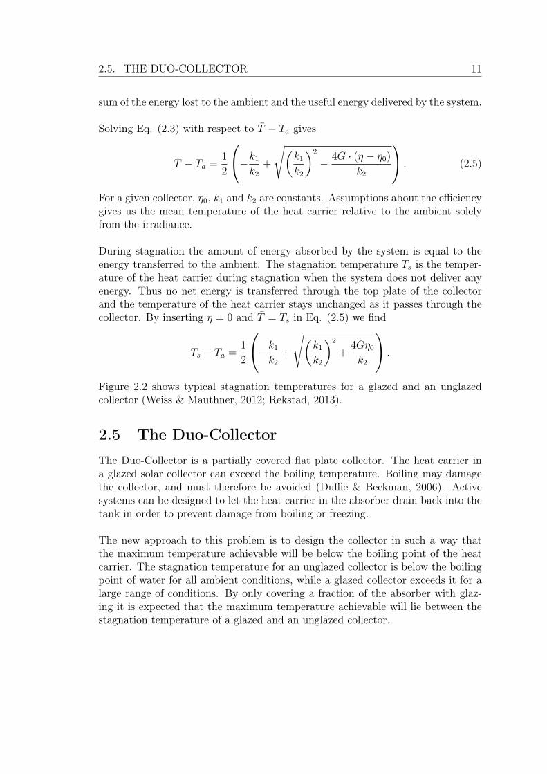
Figure 2.2 shows typical stagnation temperatures for a glazed and an unglazedcollector (Weiss & Mauthner, 2012; Rekstad, 2013).

2.5 The Duo-CollectorThe Duo-Collector is a partially covered flat plate collector. The heat carrier ina glazed solar collector can exceed the boiling temperature. Boiling may damagethe collector, and must therefore be avoided (Duffie & Beckman, 2006). Activesystems can be designed to let the heat carrier in the absorber drain back into thetank in order to prevent damage from boiling or freezing.

The new approach to this problem is to design the collector in such a way thatthe maximum temperature achievable will be below the boiling point of the heatcarrier. The stagnation temperature for an unglazed collector is below the boilingpoint of water for all ambient conditions, while a glazed collector exceeds it for alarge range of conditions. By only covering a fraction of the absorber with glaz-ing it is expected that the maximum temperature achievable will lie between thestagnation temperature of a glazed and an unglazed collector.


0 200 400 600 800 1000 12000

20

40

60

80

100

120

140

Irradiance [W/m2]

Stagnation temperature above ambient [

° C]

glazed

unglazed

Figure 2.2: Temperature above ambient of the absorber during stagnation. The temper-ature of the absorber is found by adding the ambient temperature.

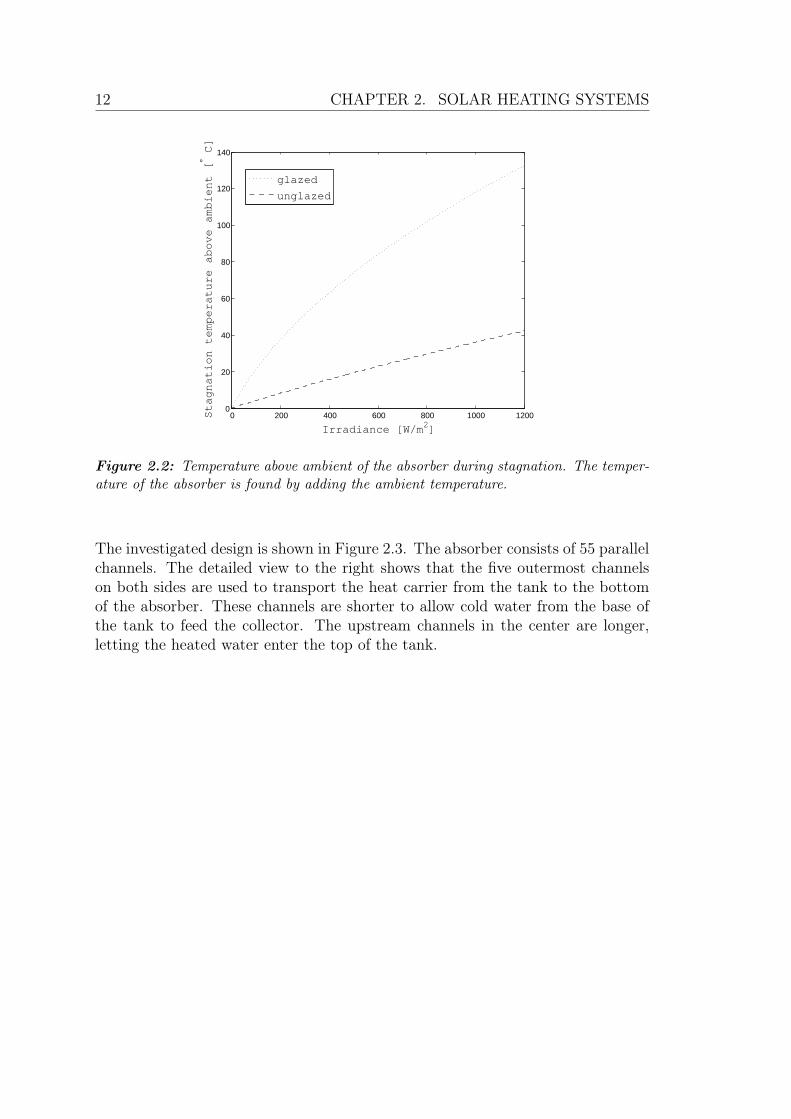
The investigated design is shown in Figure 2.3. The absorber consists of 55 parallelchannels. The detailed view to the right shows that the five outermost channelson both sides are used to transport the heat carrier from the tank to the bottomof the absorber. These channels are shorter to allow cold water from the base ofthe tank to feed the collector. The upstream channels in the center are longer,letting the heated water enter the top of the tank.

2.5. THE DUO-COLLECTOR 13

Figure 2.3: Design of the thermosyphon collector used in the simulation (HTCO GmbH,2012).

Chapter 3

Polymer science

3.1 Polypropylene

Polypropylene (PP) is a thermoplastic material with a semi-crystalline structure.Thermosplastics are a sub group of plastics and they are characterized by the factthat they soften when heated and harden when cooled. This allows them to beprocessed easily into various shapes (Wallner, Lang, & Schnetzinger, 2012; Resch& Wallner, 2012). The absorber sheets are produced by an extrusion process,where the raw material is melted, shaped in a die and then rapidly cooled downby a calibrator. This process exposes the material to high pressure and rapid tem-perature changes.

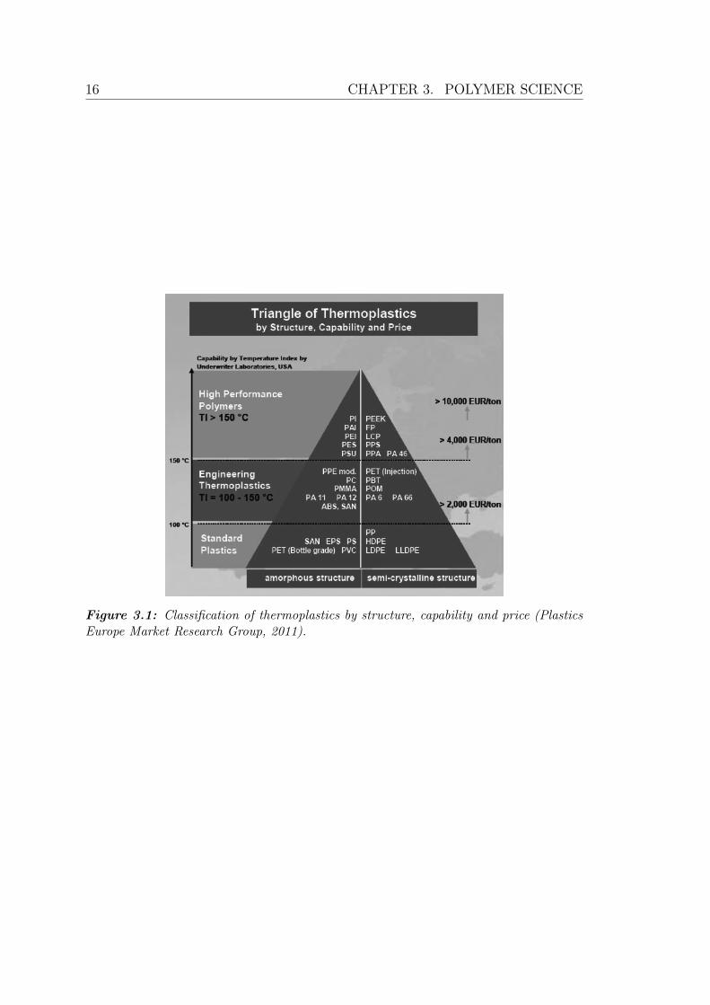
Figure 3.1 shows a classification of thermoplastics by structure, temperature per-formance and price (Plastics Europe Market Research Group, 2011). PP can befound in the bottom right cell of the pyramid. The figure shows that PP is a lowcost polymer material and is expected to tolerate temperatures up to 100 ◦C. Itis also of interest to point out that the material currently used in glazed flat platecollectors produced by Aventa is a modified PPS material, which can be found inthe top right cell.

3.2 Elasticity and plasticity

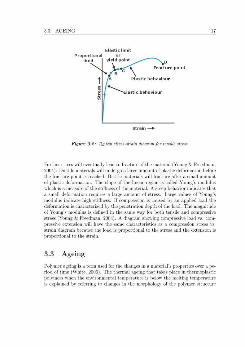
Elasticity and plasticity describes the deformation of a material when it is sub-ject to stress. Figure 3.2 shows a typical stress-strain diagram for tensile stress.The first part of the curve has a linear behavior indicating that the deformationobeys Hooke’s law. Point b in the figure indicates the elastic limit. Deformationuntil this point is reversible and beyond this point the deformation is permanent.

15

16 CHAPTER 3. POLYMER SCIENCE

Figure 3.1: Classification of thermoplastics by structure, capability and price (PlasticsEurope Market Research Group, 2011).

3.3. AGEING 17

Figure 3.2: Typical stress-strain diagram for tensile stress.

Further stress will eventually lead to fracture of the material (Young & Freedman,2004). Ductile materials will undergo a large amount of plastic deformation beforethe fracture point is reached. Brittle materials will fracture after a small amountof plastic deformation. The slope of the linear region is called Young’s moduluswhich is a measure of the stiffness of the material. A steep behavior indicates thata small deformation requires a large amount of stress. Large values of Young’smodulus indicate high stiffness. If compression is caused by an applied load thedeformation is characterized by the penetration depth of the load. The magnitudeof Young’s modulus is defined in the same way for both tensile and compressivestress (Young & Freedman, 2004). A diagram showing compressive load vs. com-pressive extension will have the same characteristics as a compression stress vs.strain diagram because the load is proportional to the stress and the extension isproportional to the strain.

3.3 Ageing

Polymer ageing is a term used for the changes in a material’s properties over a pe-riod of time (White, 2006). The thermal ageing that takes place in thermoplasticpolymers when the environmental temperature is below the melting temperatureis explained by referring to changes in the morphology of the polymer structure


(Kim, Lee, & Tsai, 2002). White (2006) presents a categorization of the differentageing processes occurring in polymers. He points out that the subject of ageingin polymers is vast, and that the categorization he makes is not sufficient to cate-gorize all topics. Still the basic features are of interest and will be presented here.

The extrusion process gives rise to physical ageing of thermoplastic polymers. Therapid cooling after the extrusion process does not leave the final product in ther-modynamic equilibrium. During the rapid cooling the material reaches thermalequilibrium with the environment. The material needs longer time to reach ther-modynamic equilibrium and the low conductivity of polymers causes the formationof a strong temperature gradient. As a result the volume of the material is largerthan it otherwise would be. The physical ageing occurs during an extended ageingperiod. Molecular relaxations over time slowly draws the material closer to equi-librium, resulting in a gradual increase of the material’s density. By increasing theageing temperature of a polymer the physical ageing may be accelerated (White,2006).

The various changes occurring in the material due to elevated temperatures, includ-ing the acceleration of physical ageing, are collectively known as thermal degra-dation. Oxygen is an aggressive chemical, which can result in scissioning andcrosslinking of the chains constituting the polymer. The rate of these reactionsare temperature dependent and may be negligible at ambient temperatures. How-ever, at elevated temperatures these reactions may occur, leading to embrittlementof the material (White, 2006).

3.4 Mathematical model of degradationThe approach which is used to describe the degradation of the absorber material atdifferent temperatures is the Arrhenius approach. By modelling the chemical pro-cesses occurring as one overall chemical process, the relation between the reactionrate χ and the temperature T in Kelvin can be expressed by:

χ(T ) = Ce−EakT , (3.1)

where C is a proportionality constant, Ea is the activation energy for the reactionand k is the Boltzmann constant. This gives a degressive rate, which means thatthe slope of the the rate is decreasing with increasing temperature. According toBockhorn, Hornung, Hornung, and Schawaller (1999) this is often the case withthe ageing process of plastics. To determine the reaction rate data from two dif-ferent temperatures are necessary. In practice it is usual to collect data for more

3.5. SERVICE LIFE ESTIMATIONS 19

than two temperatures, and use a least-squares fitting procedure to determine theconstants (Metiu, 2006).

A semi-empirical model can be used to find fitted, non-experimental values fordifferent temperatures. The model proposes that apparent mechanical changes inthe polymer reflects the changes in the molecular structure (Olivares, 2008). Itis assumed that molecular changes result in mechanical changes and compressivetests are used as the degradation parameter. The load F needed to bring thematerial to its fracture point depends on exposure temperature T and duration ofthe exposure t. The following relation is assumed

dF

dt= −χ(T )F n. (3.2)

Here the parameter n is the reaction order. According to (Rekstad & Meir, 2010)good fits are normally obtained with values of n between 1 and 2. For simplicityn = 1 and n = 2 will be used. Solving Eq. (3.2) for n = 1 gives

F (T, t) =F0

eD

and n = 2 gives

F (T, t) =1

D + 1/F0

,

where F0 is the load needed to bring unexposed material to its fracture point, andD is the thermal dose given by

D =

∫χ(T )dt.

Assuming constant temperature gives

D = χ(T )∆t.

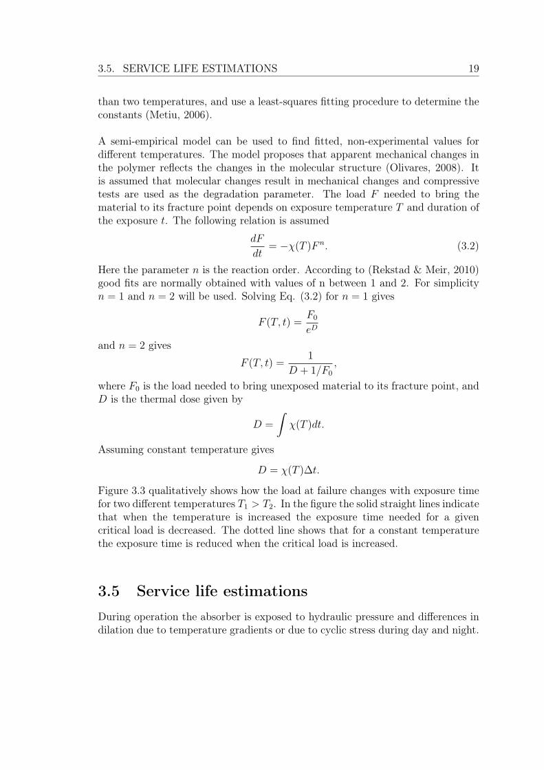
Figure 3.3 qualitatively shows how the load at failure changes with exposure timefor two different temperatures T1 > T2. In the figure the solid straight lines indicatethat when the temperature is increased the exposure time needed for a givencritical load is decreased. The dotted line shows that for a constant temperaturethe exposure time is reduced when the critical load is increased.

3.5 Service life estimationsDuring operation the absorber is exposed to hydraulic pressure and differences indilation due to temperature gradients or due to cyclic stress during day and night.


Exposure time

Loa

d at

fai

lure

t1

t2

T1

T2

Fc’

Fc

t1’

Figure 3.3: Qualitative representation of how load at failure changes with exposure timeand temperature. T1 > T2

Before operation load is applied as a result of handling of the absorber during man-ufacturing and installation. In order to estimate the service life of the absorber acriteria for failure must be introduced. The criteria for failure can be defined asthe critical load Fc which the absorber should be able to withstand (Olivares, 2008).

For the temperature T1 Figure 3.3 shows that there is a time t1 corresponding tothe critical load Fc. Likewise there is a time t2 for the temperature T2. Accordingto the theory the thermal dose D is the same for specimens with the same criticalload. Therefore the critical thermal dose Dc associated with the critical load Fccan be expressed as

Dc = χ(T1) · t1 = χ(T2) · t2.By implementing Eq. 3.1 this brings us to the following result

Ea =k · ln

(t1t2

)1T1− 1

T2

Once Ea is determined the theory allows us to predict the degradation occurringat the temperature Ti. The time ti needed to give the material the critical thermaldose Dc is given by

ti = t1eEak

(1Ti

1T1

)

Chapter 4

Experimental setup

4.1 The alphameter

The alphameter is a device used to measure the solar absorptance of a surface. Itis constructed for measurements of opaque solar absorbers, and delivers rather pre-cise measurements for this purpose. The device consists of an integrating sphere,five light sources and two detectors. The integrating sphere act as a diffuser. Op-posite the detectors there is a hole in the sphere surface, in which the specimen tobe tested is placed. The integrating sphere is illuminated subsequently by the lightsources: blue, green, red and infrared light-emitting diodes (LEDs) and a tungstenhalogene lamp. The reflected LED signals are measured by a collimated silicondetector, while the reflected tungsten halogene signal is measured by a collimatedgermanium detector (Optosol, 2002). For opaque surfaces the absorption can befound from the reflectance since the energy is either absorbed or reflected (Duffie& Beckman, 2006). The absorptance is hence measured as the complimentary partof the reflectance.

The alphameter operates in a wavelength region of 0.3 − 1.4 µm, which containsmost of the solar radiation received at the surface of the earth. It has a repro-ducibility < 0.5% (Optosol, n.d.) which means that the difference between twomeasurements will be less than 0.5% with a probability of approximately 0.95.

4.2 The Instron 3345 machine

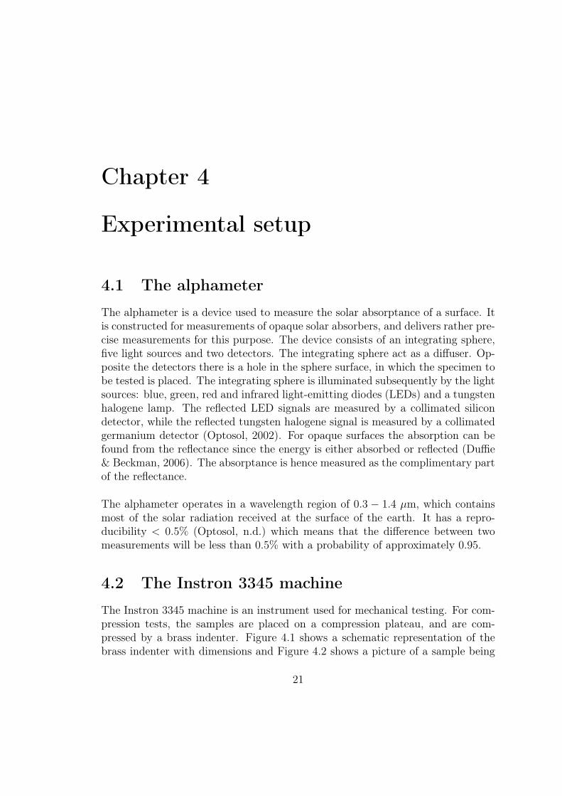
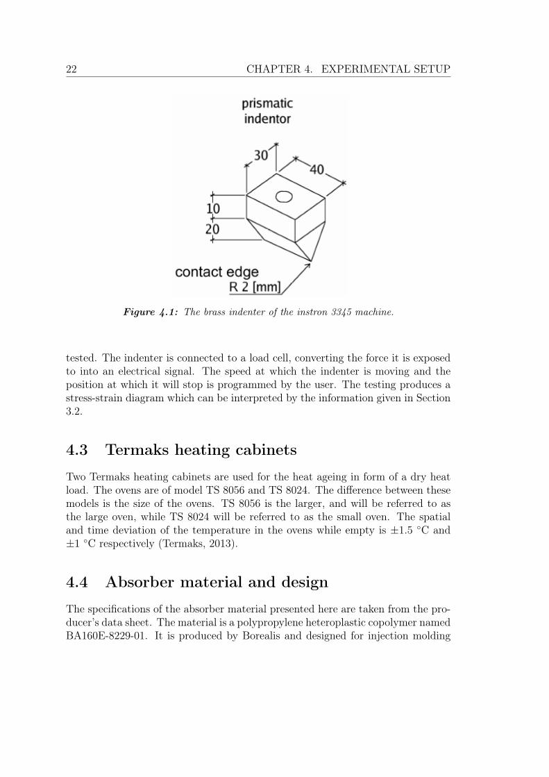
The Instron 3345 machine is an instrument used for mechanical testing. For com-pression tests, the samples are placed on a compression plateau, and are com-pressed by a brass indenter. Figure 4.1 shows a schematic representation of thebrass indenter with dimensions and Figure 4.2 shows a picture of a sample being

21

22 CHAPTER 4. EXPERIMENTAL SETUP

Figure 4.1: The brass indenter of the instron 3345 machine.

tested. The indenter is connected to a load cell, converting the force it is exposedto into an electrical signal. The speed at which the indenter is moving and theposition at which it will stop is programmed by the user. The testing produces astress-strain diagram which can be interpreted by the information given in Section3.2.

4.3 Termaks heating cabinets

Two Termaks heating cabinets are used for the heat ageing in form of a dry heatload. The ovens are of model TS 8056 and TS 8024. The difference between thesemodels is the size of the ovens. TS 8056 is the larger, and will be referred to asthe large oven, while TS 8024 will be referred to as the small oven. The spatialand time deviation of the temperature in the ovens while empty is ±1.5 ◦C and±1 ◦C respectively (Termaks, 2013).

4.4 Absorber material and design

The specifications of the absorber material presented here are taken from the pro-ducer’s data sheet. The material is a polypropylene heteroplastic copolymer namedBA160E-8229-01. It is produced by Borealis and designed for injection molding

4.4. ABSORBER MATERIAL AND DESIGN 23

Figure 4.2: Indentation test of a sample with the instron 3345 machine.

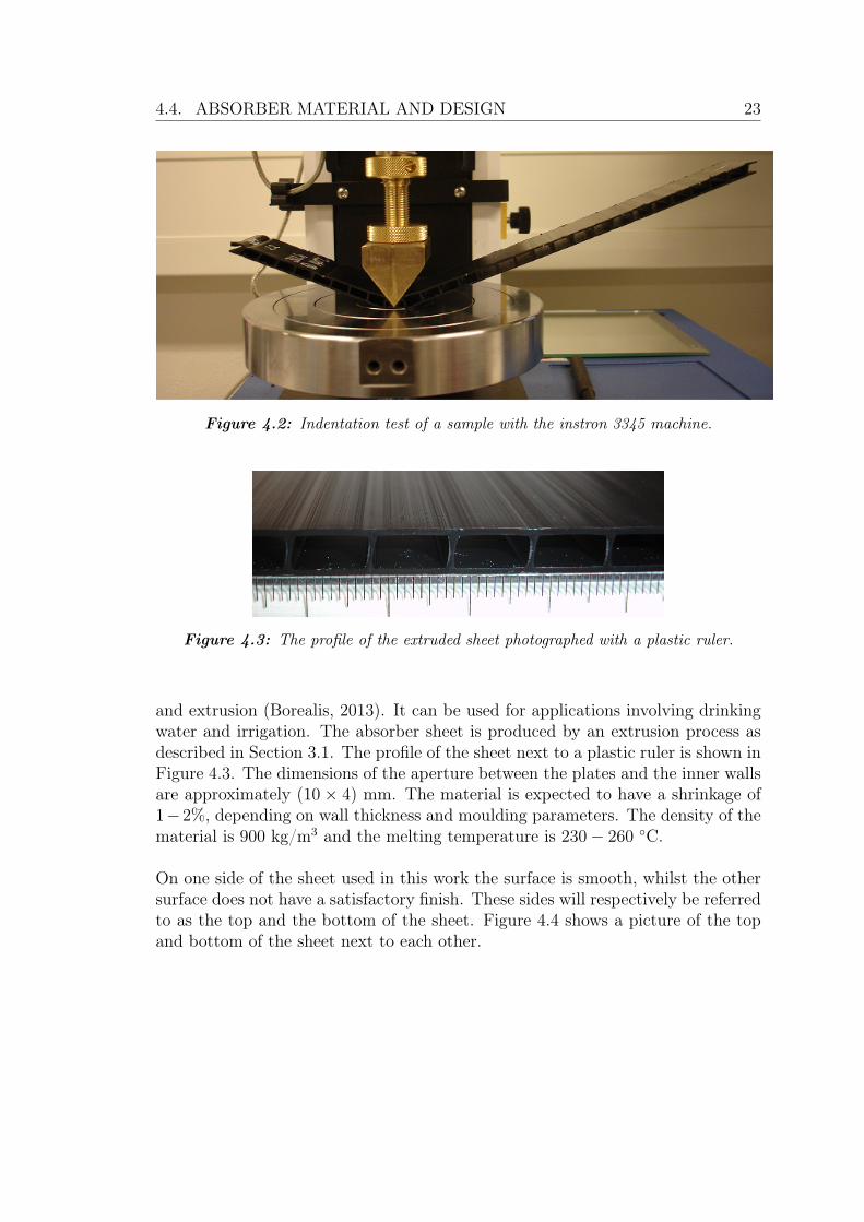
Figure 4.3: The profile of the extruded sheet photographed with a plastic ruler.

and extrusion (Borealis, 2013). It can be used for applications involving drinkingwater and irrigation. The absorber sheet is produced by an extrusion process asdescribed in Section 3.1. The profile of the sheet next to a plastic ruler is shown inFigure 4.3. The dimensions of the aperture between the plates and the inner wallsare approximately (10 × 4) mm. The material is expected to have a shrinkage of1−2%, depending on wall thickness and moulding parameters. The density of thematerial is 900 kg/m3 and the melting temperature is 230− 260 ◦C.

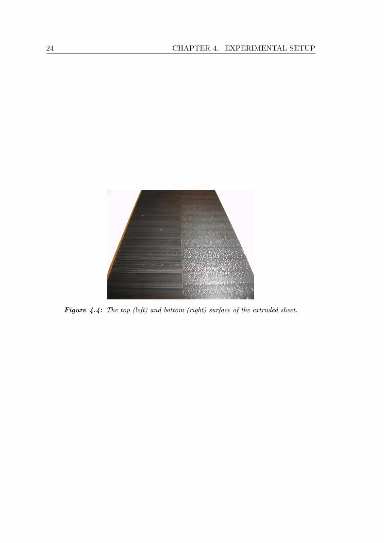
On one side of the sheet used in this work the surface is smooth, whilst the othersurface does not have a satisfactory finish. These sides will respectively be referredto as the top and the bottom of the sheet. Figure 4.4 shows a picture of the topand bottom of the sheet next to each other.

24 CHAPTER 4. EXPERIMENTAL SETUP

Figure 4.4: The top (left) and bottom (right) surface of the extruded sheet.

Chapter 5

Experimental studies

5.1 Approach

The samples

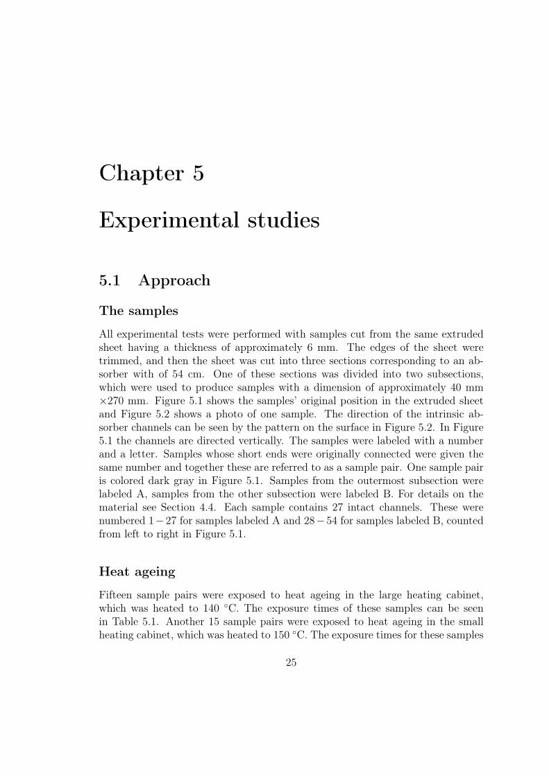
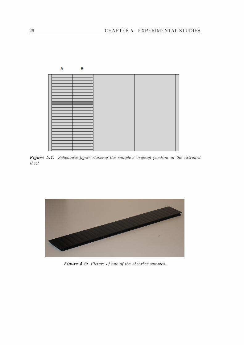
All experimental tests were performed with samples cut from the same extrudedsheet having a thickness of approximately 6 mm. The edges of the sheet weretrimmed, and then the sheet was cut into three sections corresponding to an ab-sorber with of 54 cm. One of these sections was divided into two subsections,which were used to produce samples with a dimension of approximately 40 mm×270 mm. Figure 5.1 shows the samples’ original position in the extruded sheetand Figure 5.2 shows a photo of one sample. The direction of the intrinsic ab-sorber channels can be seen by the pattern on the surface in Figure 5.2. In Figure5.1 the channels are directed vertically. The samples were labeled with a numberand a letter. Samples whose short ends were originally connected were given thesame number and together these are referred to as a sample pair. One sample pairis colored dark gray in Figure 5.1. Samples from the outermost subsection werelabeled A, samples from the other subsection were labeled B. For details on thematerial see Section 4.4. Each sample contains 27 intact channels. These werenumbered 1−27 for samples labeled A and 28−54 for samples labeled B, countedfrom left to right in Figure 5.1.

Heat ageing

Fifteen sample pairs were exposed to heat ageing in the large heating cabinet,which was heated to 140 ◦C. The exposure times of these samples can be seenin Table 5.1. Another 15 sample pairs were exposed to heat ageing in the smallheating cabinet, which was heated to 150 ◦C. The exposure times for these samples

25

26 CHAPTER 5. EXPERIMENTAL STUDIES

Figure 5.1: Schematic figure showing the sample’s original position in the extrudedsheet

Figure 5.2: Picture of one of the absorber samples.

5.1. APPROACH 27

Table 5.1: Exposure times and corresponding sample numbers for absorber samplesexposed to heat ageing at 140 ◦C. Indentation tests were carried out on the samplesmarked with a checkmark.

Exposure time Sample label Exposure time Sample label4 days = 96 h 1BX 34 days = 816 h 3A6 days = 144 h 2BX 37 days = 888 h 4A8 days = 192 h 3BX 39 days = 936 h 5A11 days = 264 h 4BX 41 days = 984 h 6A13 days = 312 h 5BX 44 days = 1056 h 7A15 days = 360 h 6BX 46 days = 1104 h 8A18 days = 432 h 7BX 48 days = 1152 h 9A20 days = 480 h 8BX 51 days = 1224 10A22 days = 528 h 9BX 53 days = 1272 h 11A25 days = 600 h 10BX 55 days = 1320 h 12A + 12B27 days = 648 h 11BX 57 days = 1368 h 13A + 13B30 days = 720 h 1A 60 days = 1440 h 14A + 14B32 days = 768 h 2A 62 days = 1488 h 15AX+ 15BX

can be seen in Table 5.2. After the exposure the samples were cooled down to roomtemperature.

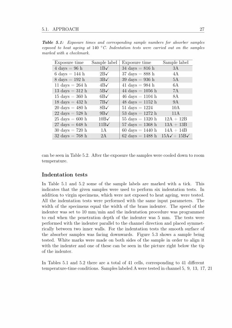
Indentation tests

In Table 5.1 and 5.2 some of the sample labels are marked with a tick. Thisindicates that the given samples were used to perform six indentation tests. Inaddition to virgin specimens, which were not exposed to heat ageing, were tested.All the indentation tests were performed with the same input parameters. Thewidth of the specimens equal the width of the brass indenter. The speed of theindenter was set to 10 mm/min and the indentation procedure was programmedto end when the penetration depth of the indenter was 5 mm. The tests wereperformed with the indenter parallel to the channel direction and placed symmet-rically between two inner walls. For the indentation tests the smooth surface ofthe absorber samples was facing downwards. Figure 5.3 shows a sample beingtested. White marks were made on both sides of the sample in order to align itwith the indenter and one of these can be seen in the picture right below the tipof the indenter.

In Tables 5.1 and 5.2 there are a total of 41 cells, corresponding to 41 differenttemperature-time conditions. Samples labeled A were tested in channel 5, 9, 13, 17, 21


Table 5.2: Exposure times and corresponding sample numbers for absorber samplesexposed to heat ageing at 150 ◦C. Indentation tests were carried out on the samplesmarked with a checkmark.

Exposure time Sample label Exposure time Sample label4 days = 96 h 16A + 16BX 22 days = 528 h 24A + 24B6 days = 144 h 17A + 17BX 25 days = 600 h 25A + 25BX8 days = 192 h 18A + 18B 27 days = 648 h 26A + 26B11 days = 264 h 19A + 19B 29 days = 696 h 27A + 27B13 days = 312 h 20A + 20B 32 days = 768 h 28A + 28B15 days = 360 h 21A + 21BX 34 days = 816 h 29A + 29B18 days = 432 h 22A + 22B 36 days = 864 h 30AX+ 30BX20 days = 480 h 23A + 23B

Figure 5.3: Picture of a sample during an indentation test.

5.1. APPROACH 29

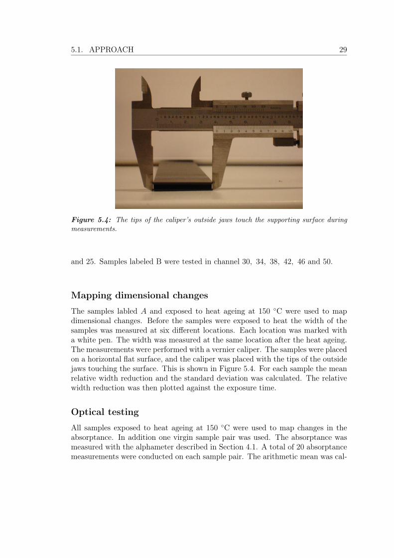
Figure 5.4: The tips of the caliper’s outside jaws touch the supporting surface duringmeasurements.

and 25. Samples labeled B were tested in channel 30, 34, 38, 42, 46 and 50.

Mapping dimensional changes

The samples labled A and exposed to heat ageing at 150 ◦C were used to mapdimensional changes. Before the samples were exposed to heat the width of thesamples was measured at six different locations. Each location was marked witha white pen. The width was measured at the same location after the heat ageing.The measurements were performed with a vernier caliper. The samples were placedon a horizontal flat surface, and the caliper was placed with the tips of the outsidejaws touching the surface. This is shown in Figure 5.4. For each sample the meanrelative width reduction and the standard deviation was calculated. The relativewidth reduction was then plotted against the exposure time.

Optical testing

All samples exposed to heat ageing at 150 ◦C were used to map changes in theabsorptance. In addition one virgin sample pair was used. The absorptance wasmeasured with the alphameter described in Section 4.1. A total of 20 absorptancemeasurements were conducted on each sample pair. The arithmetic mean was cal-


−1 0 1 2 3 4 5 6−500

0

500

1000

1500

2000

2500

3000

3500

Compressive extension [mm]

Compressive load [N]

1488h at 140°C

864h at 150°C

virgin sheet

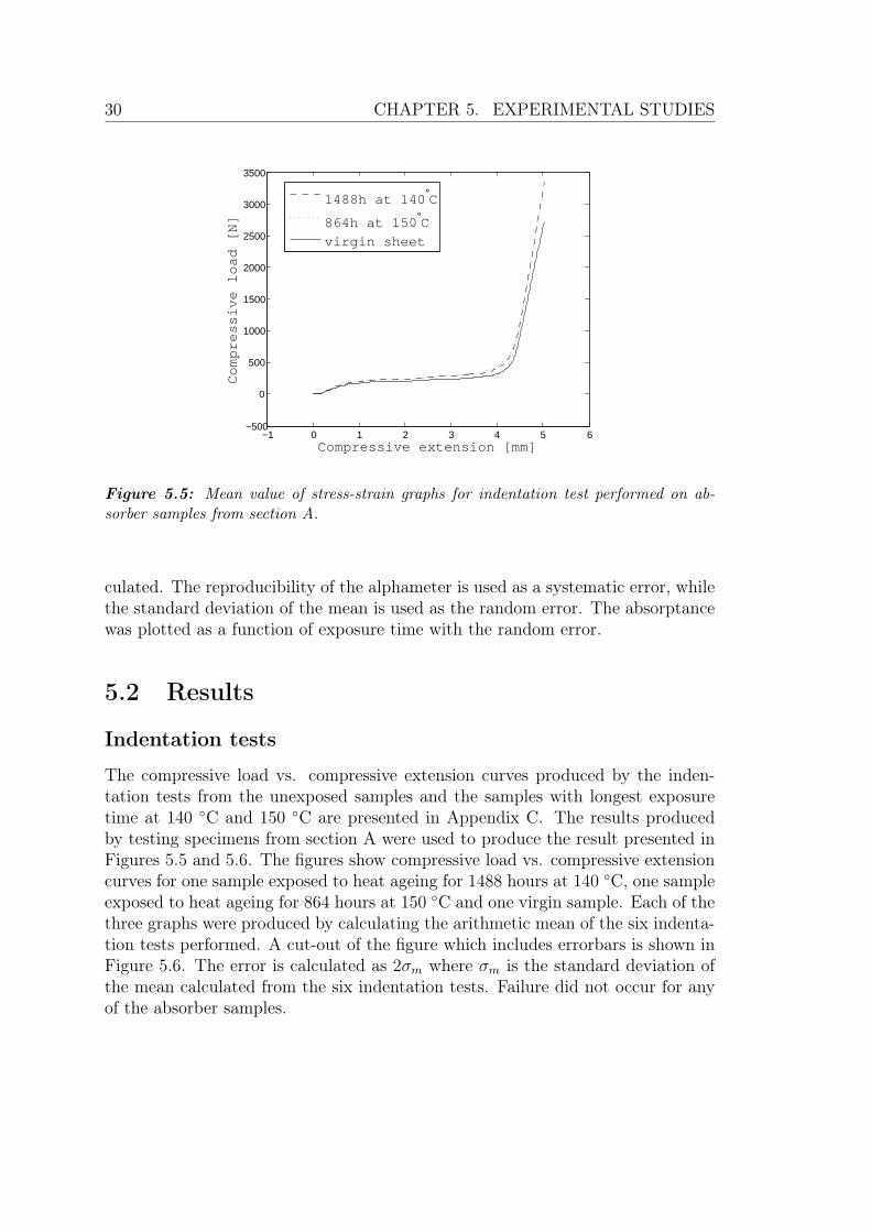
Figure 5.5: Mean value of stress-strain graphs for indentation test performed on ab-sorber samples from section A.

culated. The reproducibility of the alphameter is used as a systematic error, whilethe standard deviation of the mean is used as the random error. The absorptancewas plotted as a function of exposure time with the random error.

5.2 Results

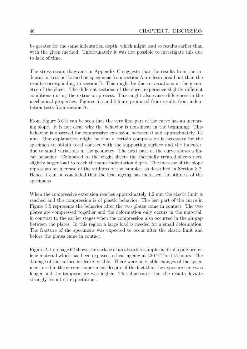
Indentation tests

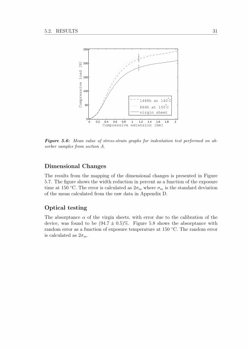
The compressive load vs. compressive extension curves produced by the inden-tation tests from the unexposed samples and the samples with longest exposuretime at 140 ◦C and 150 ◦C are presented in Appendix C. The results producedby testing specimens from section A were used to produce the result presented inFigures 5.5 and 5.6. The figures show compressive load vs. compressive extensioncurves for one sample exposed to heat ageing for 1488 hours at 140 ◦C, one sampleexposed to heat ageing for 864 hours at 150 ◦C and one virgin sample. Each of thethree graphs were produced by calculating the arithmetic mean of the six indenta-tion tests performed. A cut-out of the figure which includes errorbars is shown inFigure 5.6. The error is calculated as 2σm where σm is the standard deviation ofthe mean calculated from the six indentation tests. Failure did not occur for anyof the absorber samples.

5.2. RESULTS 31

0 0.2 0.4 0.6 0.8 1 1.2 1.4 1.6 1.8 20

50

100

150

200

250



1488h at 140°C

864h at 150°C

virgin sheet

Figure 5.6: Mean value of stress-strain graphs for indentation test performed on ab-sorber samples from section A.

Dimensional Changes

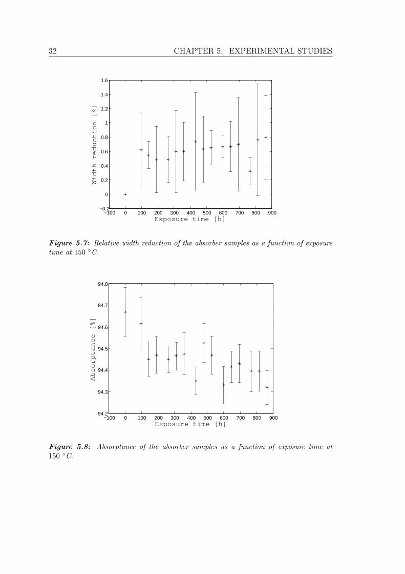
The results from the mapping of the dimensional changes is presented in Figure5.7. The figure shows the width reduction in percent as a function of the exposuretime at 150 ◦C. The error is calculated as 2σm where σm is the standard deviationof the mean calculated from the raw data in Appendix D.

Optical testing

The absorptance α of the virgin sheets, with error due to the calibration of thedevice, was found to be (94.7 ± 0.5)%. Figure 5.8 shows the absorptance withrandom error as a function of exposure temperature at 150 ◦C. The random erroris calculated as 2σm.


−100 0 100 200 300 400 500 600 700 800 900−0.2

0

0.2

0.4

0.6

0.8

1

1.2

1.4

1.6

Exposure time [h]

Width reduction [%]

Figure 5.7: Relative width reduction of the absorber samples as a function of exposuretime at 150 ◦C.

−100 0 100 200 300 400 500 600 700 800 90094.2

94.3

94.4

94.5

94.6

94.7

94.8

Exposure time [h]

Absorptance [%]

Figure 5.8: Absorptance of the absorber samples as a function of exposure time at150 ◦C.

Chapter 6

Simulation

6.1 ApproachThe simulation developed in this master’s thesis calculates the maximum temper-atures obtainable in a Duo-Collector and investigate the performance of such asystem. The terms defined below will be used in the following:

• the glazing fraction referres to the percentage of the absorber covered withglazing and will be denoted P . P = 0 corresponds to an unglazed collector,while P = 100 corresponds to a glazed collector.

• the relative temperature equals the actual temperature minus the ambi-ent temperature.

• the temperature rise equals the difference between the outlet temperatureand the inlet temperature.

• the velocity will refer to the magnitude of the velocity of the heat carrierin the upstream region of the collector.

• the no-gain temperature will refer to the temperature when the temper-ature rise equals zero.

• the stagnation temperature will refer to the temperature when the ve-locity equals zero.

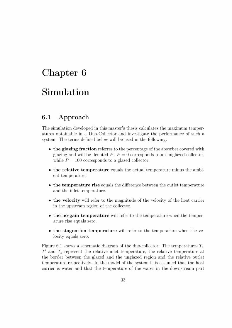
Figure 6.1 shows a schematic diagram of the duo-collector. The temperatures Ti,T ′ and To represent the relative inlet temperature, the relative temperature atthe border between the glazed and the unglazed region and the relative outlettemperature respectively. In the model of the system it is assumed that the heatcarrier is water and that the temperature of the water in the downstream part

33

34 CHAPTER 6. SIMULATION

Figure 6.1: Schematic diagram of the Duo-Collector

of the absorber is constant. Further the model assumes steady state conditionsand that the temperature in the upstream channels only changes in the y-direction.

The simulation consists of four MATLAB programs. The programs can be found inAppendix B. The following subsections present the derivations of the mathematicalrelations used in the simulation and descriptions of the programs. The input valuesused for the simulation can be seen in Table 6.1.

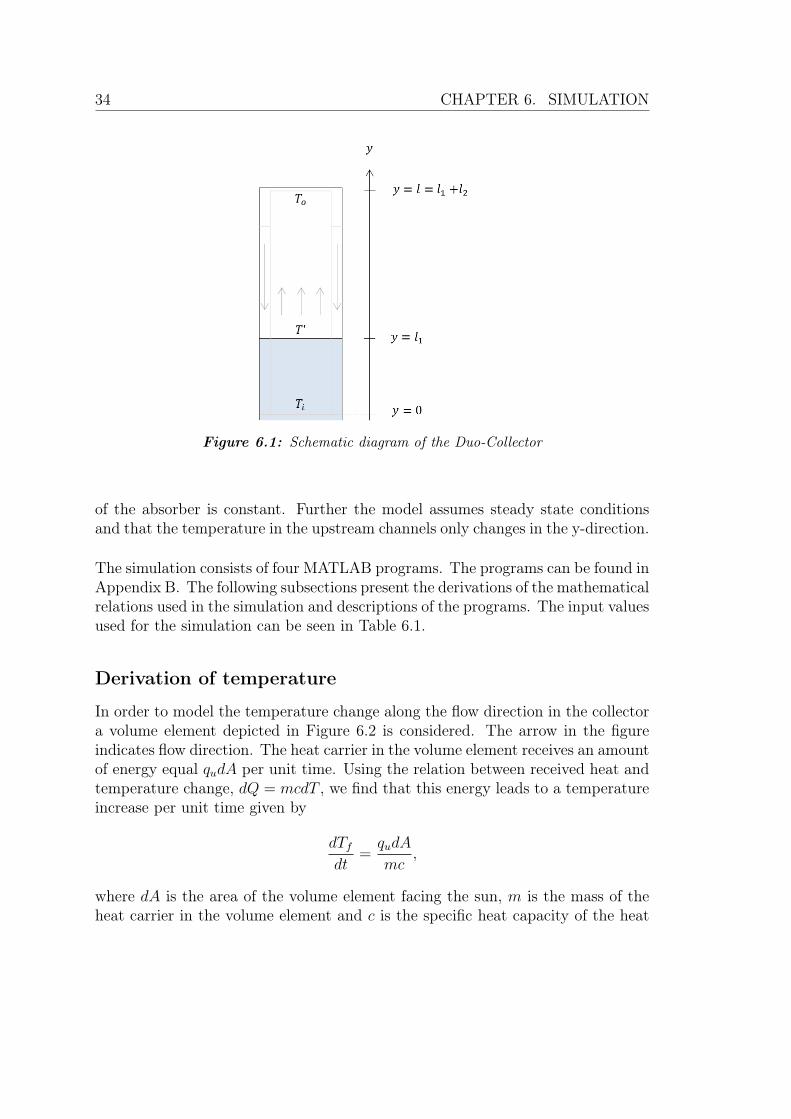
Derivation of temperature

In order to model the temperature change along the flow direction in the collectora volume element depicted in Figure 6.2 is considered. The arrow in the figureindicates flow direction. The heat carrier in the volume element receives an amountof energy equal qudA per unit time. Using the relation between received heat andtemperature change, dQ = mcdT , we find that this energy leads to a temperatureincrease per unit time given by

dTfdt

=qudA

mc,

where dA is the area of the volume element facing the sun, m is the mass of theheat carrier in the volume element and c is the specific heat capacity of the heat

6.1. APPROACH 35

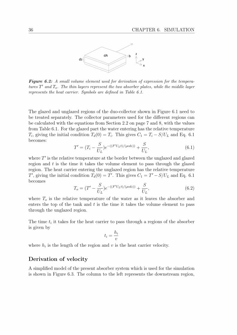
Table 6.1: Values used for simulation

Description Symbol value

aperture between the innerwalls of the absorber sheet dx 1 cm

aperture between the absorber sheet plates dz 4 mm

height of absorber h 3 m

ambient temperature Ta 20 ◦C

absorptance of absorber sheet α 0.947

transmittance of glazing τ 0.84

specific heat capacity of water c 4181 J/(kgK)

thickness of the absorber sheet plates b 0.8 mm

density of water ρ 1000 kg/m3

thermal conductivity of absorber material k 0.2 W/(mK)

back loss coefficient Ub 1.4 W/(m2K)

fraction of absorber which is glazed P 0− 100%

radiance incident on absorber G 0− 1200 W/m2

carrier. Using the fact that m = ρV = ρdAdz and applying Eq. 2.1, we find that

dTfdt

=1

ρcdzF ′[S − UL(Tf − Ta)].

By introducing the relative temperature Td = Tf − Ta, being the temperaturedifference between the heat carrier temperature and the ambient temperature, Eq.(6.1) gives

Tddt

=1

ρcdzF ′[S − ULTd].

This is a linear differential equation leading to the following solution:

Td =S

UL+ C1e

−((F ′ULt)/(ρcdz)),

where C1 is a constant of integration.


b dz

dA z

y

x

Figure 6.2: A small volume element used for derivation of expression for the tempera-tures T ′ and To. The thin layers represent the two absorber plates, while the middle layerrepresents the heat carrier. Symbols are defined in Table 6.1.

The glazed and unglazed regions of the duo-collector shown in Figure 6.1 need tobe treated separately. The collector parameters used for the different regions canbe calculated with the equations from Section 2.2 on page 7 and 8, with the valuesfrom Table 6.1. For the glazed part the water entering has the relative temperatureTi, giving the initial condition Td(0) = Ti. This gives C1 = Ti− S/UL and Eq. 6.1becomes:

T ′ = (Ti −S

UL)e−((F ′ULt)/(ρcdz)) +

S

UL, (6.1)

where T ′ is the relative temperature at the border between the unglazed and glazedregion and t is the time it takes the volume element to pass through the glazedregion. The heat carrier entering the unglazed region has the relative temperatureT ′, giving the initial condition Td(0) = T ′. This gives C1 = T ′−S/UL and Eq. 6.1becomes

To = (T ′ − S

UL)e−((F ′ULt)/(ρcdz)) +

S

UL, (6.2)

where To is the relative temperature of the water as it leaves the absorber andenters the top of the tank and t is the time it takes the volume element to passthrough the unglazed region.

The time ti it takes for the heat carrier to pass through a regions of the absorberis given by

ti =hiv

where hi is the length of the region and v is the heat carrier velocity.

Derivation of velocity

A simplified model of the present absorber system which is used for the simulationis shown in Figure 6.3. The column to the left represents the downstream region,

6.1. APPROACH 37

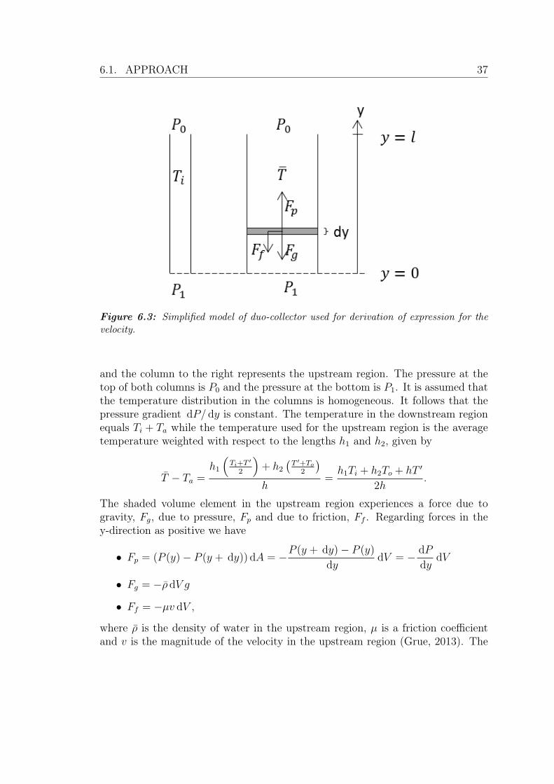
Figure 6.3: Simplified model of duo-collector used for derivation of expression for thevelocity.

and the column to the right represents the upstream region. The pressure at thetop of both columns is P0 and the pressure at the bottom is P1. It is assumed thatthe temperature distribution in the columns is homogeneous. It follows that thepressure gradient dP/ dy is constant. The temperature in the downstream regionequals Ti + Ta while the temperature used for the upstream region is the averagetemperature weighted with respect to the lengths h1 and h2, given by

T̄ − Ta =h1

(Ti+T

′

2

)+ h2

(T ′+To

2

)h

=h1Ti + h2To + hT ′

2h.

The shaded volume element in the upstream region experiences a force due togravity, Fg, due to pressure, Fp and due to friction, Ff . Regarding forces in they-direction as positive we have

• Fp = (P (y)− P (y + dy)) dA = −P (y + dy)− P (y)

dydV = − dP

dydV

• Fg = −ρ̄ dV g

• Ff = −µv dV ,

where ρ̄ is the density of water in the upstream region, µ is a friction coefficientand v is the magnitude of the velocity in the upstream region (Grue, 2013). The


element does not experience any acceleration, hence∑F = 0⇒ dP

dy+ ρ̄g + µv = 0

Rearranging this equations leads us to an expression for the speed v:

v = − 1

µ

(dP

dy+ ρ̄g

). (6.3)

Next the downstream column is used to find the pressure gradient. With the useof Eq. (2.4) on page 10 we find that

dP

dy=P0 − P1

h=P0 − (P0 + ρigh))

h= −ρig,

where ρi is the density of water at temperature Ti +Ta. Inserting this into Eq. 6.3leads us to the expression for the velocity:

v =1

µ(ρi − ρ̄)g. (6.4)

The density of water as a function of temperature was found by fitting tabulatedvalues (CRC Press, 2005) with a second order polynomial.

Modelling the temperature

The program temp.m found in Appendix B is used to calculate the temperaturedistribution in the collector. The following input parameters must be specified torun the program:

• The irradiance, G

• The glazing fraction, P

• The relative inlet temperature, Ti

• The velocity of the heat carrier , v

The other parameters needed to carry out the calculations are specified in theprogram and can be found in Table 6.1. The program uses Eq. 6.1 to find thetemperature at the border, T ′, which is then used to find the outlet temperatureTo with the use of equation 6.2.

The program returns the following parameters:

6.1. APPROACH 39

• The vector T which contains the temperatures Ti, Tb and To

• The vector h which contains the heights h1 and h2 specified in Figure 6.1

For an unglazed and a glazed collector the top loss coefficients are fitted so thatthe relative stagnation temperatures of the systems at G = 1000 W/m2 is 40 Kand 120 K respectively.

Modelling the flow velocity

The function velocity.m found in Appendix B is used to calculate the heat carriervelocity. The program takes the following input parameters:

• The vector T which includes the three temperatures Ti, Tb and To

• The vector h which includes the two heigths h1 and h2

The program uses Eq. (6.4) from page 38 to calculate the velocity v. The frictioncoefficient µ is fitted so that heat carrier with Ti = 0 and Ta = 20◦C runningthrough a glazed collector exposed to an irradiance of 1000 W/m2 has a temera-ture rise of approximately 10 K. The program returns v.

Modelling no-gain temperature

The program no_gain.m found in Appendix B calculates the no-gain temperaturerelative to the ambient temperature for different irradiance levels. The calculationsare performed for an unglazed collector (P = 0%), collectors with glazing cover-ing 25%, 50% and 75% of the absorber and a fully glazed collector (P = 100%).For a given irradiance and cover fraction, the functions temp.m and velocity.mare used in an iterative procedure. The program continues until the steady statesituation when the inlet and outlet temperature are equal is reached. The no-gaintemperature is defined as the temperature at the border between the glazed andthe unglazed region during no-gain conditions. The no-gain temperatures for thedifferent collectors are then presented graphically as functions of irradiance.

Modelling the efficiency

The program efficiency.m found in Appendix B produces graphs showing how theefficiency varies with the mean temperature in the collector and how the temper-ature rise through the collector and the velocity of the heat carrier vary with the


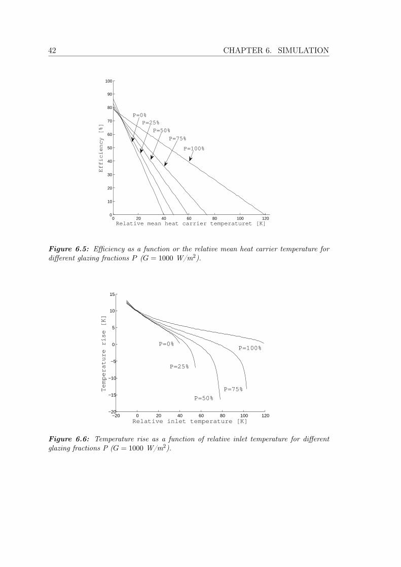
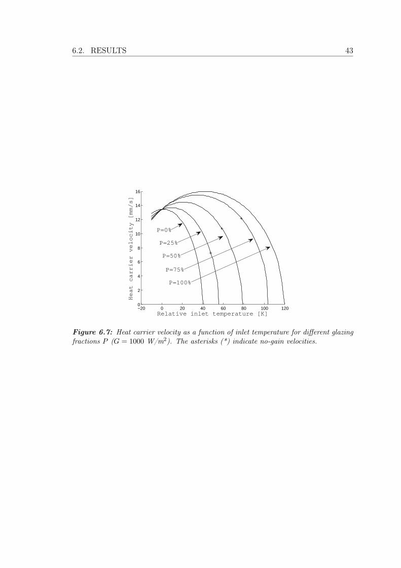
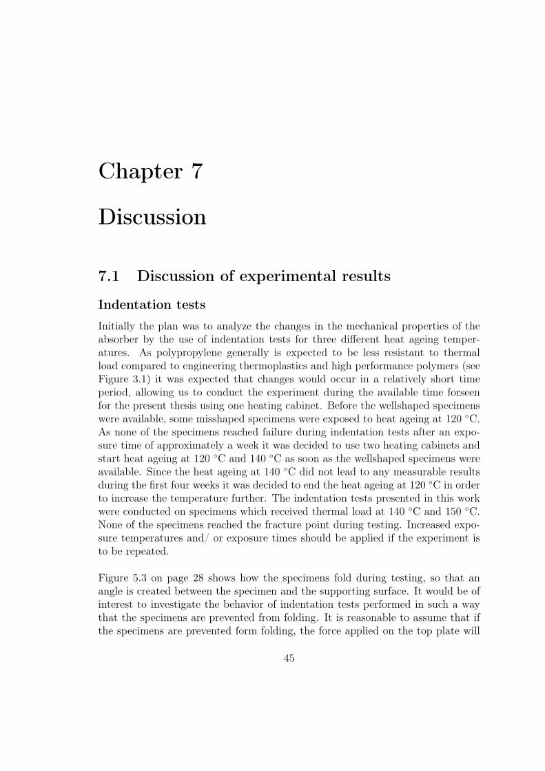
inlet temperature. Also, a selection of efficiencies are calculated for different out-let temperatures. All the calculations are done for G = 1000 W/m2 for differentglazing fraction.

To calculate the efficiency we considering a time interval t. The total useful gainduring the time t can be expressed as

Total useful gain = vAc∆Tct/ρ.

∆T is the temperature rise through the collector given by To − Ti and Ac is thecross section of the upstream channels perpendicular to the flow direction. Thesolar energy received is given by

Solar energy received = AGt,

where A is the area receiving solar energy. In the calculations presented here thearea A is defined as the contact area between the heat carrier and the top plate.By employing Eq. (2.2) on page 8 we find that the efficiency is given by

η =vAc∆Tc

ρAG.

6.2 ResultsThe fitting of the parameters Ut and µ can be found in Table 6.2. Figure 6.4 showsthe no-gain temperature above ambient temperature as a function of irradiancefor collectors with different glazing fractions. Figure 6.5 shows the efficiency ofcollectors with different glazing fractions as a function of the relative mean heatcarrier temperature. The efficiency for some outlet temperatures and glazing frac-tions are presented in Table 6.3. The temperature rise and the velocity of the heatcarrier as a function of the inlet temperature can be seen in Figures 6.6 and 6.7.All the results are calculated with Ta = 20 ◦C.

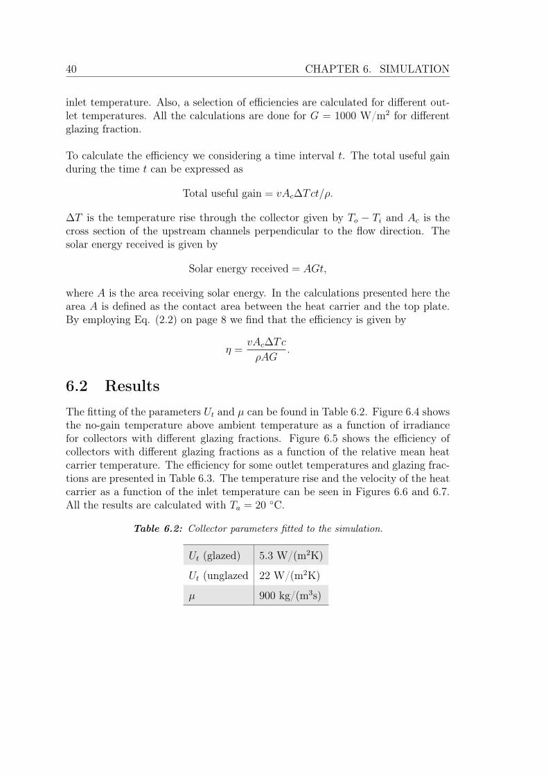
Table 6.2: Collector parameters fitted to the simulation.

Ut (glazed) 5.3 W/(m2K)

Ut (unglazed 22 W/(m2K)

µ 900 kg/(m3s)

6.2. RESULTS 41

0 200 400 600 800 1000 12000

50

100

150

Irradiance [W/m 2]

Re

lativ

e n

o−

ga

in t

em

pe

ratu

re [

K]

P=50%

P=75%

P=100%

P=25%

P=0%

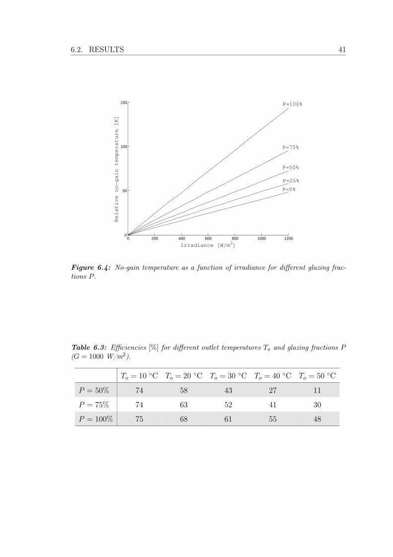
Figure 6.4: No-gain temperature as a function of irradiance for different glazing frac-tions P .

Table 6.3: Efficiencies [%] for different outlet temperatures To and glazing fractions P(G = 1000 W/m2).

To = 10 ◦C To = 20 ◦C To = 30 ◦C To = 40 ◦C To = 50 ◦C

P = 50% 74 58 43 27 11

P = 75% 74 63 52 41 30

P = 100% 75 68 61 55 48


0 20 40 60 80 100 1200

10

20

30

40

50

60

70

80

90

100

Relative mean heat carrier temperaturet [K]

Efficiency [%]

P=0%P=25%

P=50%

P=75%

P=100%

Figure 6.5: Efficiency as a function or the relative mean heat carrier temperature fordifferent glazing fractions P (G = 1000 W/m2).

−20 0 20 40 60 80 100 120−20

−15

−10

−5

0

5

10

15

Relative inlet temperature [K]

Temperature rise [K]

P=100%

P=50%

P=25%

P=0%

P=75%

Figure 6.6: Temperature rise as a function of relative inlet temperature for differentglazing fractions P (G = 1000 W/m2).

6.2. RESULTS 43

−20 0 20 40 60 80 100 1200

2

4

6

8

10

12

14

16

Relative inlet temperature [K]

Heat carrier velocity [mm/s]

P=100%

P=75%

P=50%

P=25%

P=0%

Figure 6.7: Heat carrier velocity as a function of inlet temperature for different glazingfractions P (G = 1000 W/m2). The asterisks (*) indicate no-gain velocities.

Chapter 7

Discussion

7.1 Discussion of experimental results

Indentation tests

Initially the plan was to analyze the changes in the mechanical properties of theabsorber by the use of indentation tests for three different heat ageing temper-atures. As polypropylene generally is expected to be less resistant to thermalload compared to engineering thermoplastics and high performance polymers (seeFigure 3.1) it was expected that changes would occur in a relatively short timeperiod, allowing us to conduct the experiment during the available time forseenfor the present thesis using one heating cabinet. Before the wellshaped specimenswere available, some misshaped specimens were exposed to heat ageing at 120 ◦C.As none of the specimens reached failure during indentation tests after an expo-sure time of approximately a week it was decided to use two heating cabinets andstart heat ageing at 120 ◦C and 140 ◦C as soon as the wellshaped specimens wereavailable. Since the heat ageing at 140 ◦C did not lead to any measurable resultsduring the first four weeks it was decided to end the heat ageing at 120 ◦C in orderto increase the temperature further. The indentation tests presented in this workwere conducted on specimens which received thermal load at 140 ◦C and 150 ◦C.None of the specimens reached the fracture point during testing. Increased expo-sure temperatures and/ or exposure times should be applied if the experiment isto be repeated.

Figure 5.3 on page 28 shows how the specimens fold during testing, so that anangle is created between the specimen and the supporting surface. It would be ofinterest to investigate the behavior of indentation tests performed in such a waythat the specimens are prevented from folding. It is reasonable to assume that ifthe specimens are prevented form folding, the force applied on the top plate will

45

46 CHAPTER 7. DISCUSSION

be greater for the same indentation depth, which might lead to results earlier thanwith the given method. Unfortunately it was not possible to investigate this dueto lack of time.

The stress-strain diagrams in Appendix C suggests that the results from the in-dentation test performed on specimens from section A are less spread out than theresults corresponding to section B. This might be due to variations in the geom-etry of the sheet. The different sections of the sheet experience slightly differentconditions during the extrusion process. This might also cause differences in themechanical properties. Figures 5.5 and 5.6 are produced from results from inden-tation tests from section A.

From Figure 5.6 it can be seen that the very first part of the curve has an increas-ing slope. It is not clear why the behavior is non-linear in the beginning. Thisbehavior is observed for compressive extension between 0 and approximately 0.2mm. One explanation might be that a certain compression is necessary for thespecimen to obtain total contact with the supporting surface and the indenter,due to small variations in the geometry. The next part of the curve shows a lin-ear behavior. Compared to the virgin sheets the thermally treated sheets needslightly larger load to reach the same indentation depth. The increase of the sloperepresents an increase of the stiffness of the samples, as described in Section 3.2.Hence it can be concluded that the heat ageing has increased the stiffness of thespecimens.

When the compressive extension reaches approximately 1.2 mm the elastic limit isreached and the compression is of plastic behavior. The last part of the curve inFigure 5.5 represents the behavior after the two plates come in contact. The twoplates are compressed together and the deformation only occurs in the material,in contrast to the earlier stages when the compression also occurred in the air gapbetween the plates. In this region a large load is needed for a small deformation.The fracture of the specimens was expected to occur after the elastic limit andbefore the plates came in contact.

Figure A.1 on page 62 shows the surface of an absorber sample made of a polypropy-lene material which has been exposed to heat ageing at 130 ◦C for 115 hours. Thedamage of the surface is clearly visible. There were no visible changes of the speci-mens used in the current experiment despite of the fact that the exposure time waslonger and the temperature was higher. This illustrates that the results deviatestrongly from first expectations.

7.1. DISCUSSION OF EXPERIMENTAL RESULTS 47

Da Silva (2008) investigated how results of the indentation tests depend on thewidth of the tested specimens. The results presented in Figure A.3 are from in-dentation tests on virgin specimens made of PPS. They show that the slope of thelinear region increases with increasing width. Comparing the curve correspondingto tests done on specimens with a width of 48 mm and performed on the topsurface with the solid line in Figure 5.6 we see that for indentation depths of 0.5mm the loads are approximately 140 N and 100 N respectively. Hence the slope ofthe indentation curves of the PP absorber is slightly smaller. Taking into accountthat da Silva’s specimens are slightly wider we can conclude that the stiffness ofthe PP absorber tested in this work and the PPS absorber tested by da Silva areof similar size.

Figure A.2 shows the result from indentation tests performed on a PPE/PS blend.These can be found in the bottom and middle left cells in the pyramid shown inFigure 3.1 on page 16. The width of the specimens tested were from 72− 87 mm.Compared to the results of samples with a width of 81 mm from Figure A.3 we seethat the stiffness of the PPE/PS specimens is larger than that of the PPS. Theincreased stiffness leads to a larger indentation load during the region where frac-ture is expected to occur. Stiffness depends on the shape as well as the material.Since the absorber sheet made of the PPE/PS material was a triple-wall sheet wecannot draw conclusions about the stiffness of the materials relative to each other.This shows that the design parameters are of great importance for the results ofindentation tests.

The absorber samples made of the material BA160E clearly withstands exposureto dry heat load better than expected from previous studies om PP materials.It would be intersting to compare to which extent the present PP specimens cansustain dry heat ageing in comparison to PPS specimens. Further investigationsare needed to give quantitative results.

Dimensional changes

The mapping of the dimensional changes was done on the absorber samples whichwere exposed to heat ageing at 150 ◦C. The reduction in width for the differentexposure times are presented in Figure 5.7. The measuring point correspondingto an exposure time of 768 h clearly stands out. In the raw data presented inAppendix D it can be seen that the difference in the width on location e for thegiven exposure time is the only negative value, which corresponds to an increaseof the width as a result of the heat ageing. A total of 180 measurements wereperformed to produce the raw data. It is likely that this is a measurement error.The first point in Figure 5.7 is not a measurement point. As this point represents


the reduction in width for a virgin absorber it must be zero to make physical sense.

Although the measurement points do not give a clear correlation between the ex-posure time and the reduction in width they indicate that the reduction mainlyoccurs in the early stages of the heat exposure. According to the theory presentedin Section 3.3 physical ageing due to molecular relaxations lead to a reduction ofthe materials volume. Since the molecular relaxation gradually draws the materialcloser to equilibrium the rate is expected to be degressive (decrease with time)leading to a more significant change in the beginning. This is in agreement withthe measured results as the difference between the first and the second point inFigure 5.7 is large compaired to the the difference between the rest of the points.This behavior also suggests that most of the reduction has occurred within theearly stages of the heat ageing. By decreasing the time interval between the mea-surement points, especially in the region between 0 and 96 hours, the behaviorcould be mapped with greater detail.

The cause of the errors might be local variations both in the composition of thematerial and the geometry. The reduction is measured to be less than 1%. As theexpected value was between 1% and 2% this is a satisfying result.

Optical testing

The absorptance as a function of exposure time at 150 ◦C is shown in Figure 5.8.As the aim was to study the change in absorptance of the absorber the systematicerror caused by the calibration of the alphameter is not included in the figure. Thiserror is much larger than the errors presented in the figure and it is important toinclude the calibration error when considering the certainty of the measured val-ues in comparison to other material surfaces. The samples used for the currentexperiment were also used for mapping the dimensional changes, and some werealso used to perform indentation tests. The handling of the samples might haveaffected the results, for example by causing the surface to be scratches or soiled.

The results show a decrease in the absorptance as a function of exposure time. Theexposure times were up to about five weeks, and during this time the reduction inabsorptance was less than 0.4%. The values presented in Table A.1 in Appendix Ashow absorptance measurements performed on PPS absorber samples. The valuesare presented for different wavelengths. All the values are below the measuredabsorptance of the material tested in the current work, which was (94.7 ± 0.5)%.Since the solar energy absorbed by a flat plate collector is proportional to theabsorptance it is preferrable with high absorptance values. The absorptance of thesurface of the absorber shows satisfying absorptance properties for solar thermal

7.2. DISCUSSION OF RESULTS FROM SIMULATION 49

applications.

7.2 Discussion of results from simulation

The simulation programs developed were fitted to fit the empirical behavior ofunglazed and glazed collectors. Still, the program is based on a number of as-sumptions. It is therefore important to emphasize that the results produced bythe programs might deviate from the actual behavior of a Duo-Collector. Themodel should be compared with empirical behavior to be verified.

No-gain temperature

The no-gain temperature as a function of irradiance for collectors with differentglazing fractions is presented in Figure 6.4. The figure shows that there is not alinear relation between the glazing fraction and the no-gain temperature; a col-lector with a glazing fraction of 50% has a no-gain temperature which lies closerto the stagnation temperature of an unglazed collector than to that of a glazedcollector. An interpretation of this can be found by looking at the mathematicalbasis of the simulation. Let Tg and Tu be the stagnation temperatures for a glazedand an unglazed collector respectively and consider a collector with glazing frac-tion equal 50%. Next we let the mean heat carrier temperature in this collectorbe (Tg + Tu)/2. The absorbed energy is not affected by the temperature changeof the fluid. This means that the absorbed energy equals the sum of the absorbedenergy for the two different regions. The heat loss on the other hand depends onthe temperature difference between the mean heat carrier temperature and theambient. The loss from the unglazed region of the Duo-Collector will therefore belarger than the loss from an unglazed collector during no-gain conditions. Sim-ilarly, the heat loss from the glazed region of the partially covered collector willbe smaller than the loss from a glazed collector at stagnation. If the reductionin heat loss was to compensate the increase in heat loss (Tg + Tu)/2 would bethe no-gain temperature since the net energy budget would be zero. This is notthe case because the heat loss coefficient for the unglazed part is larger than thatof the glazed part. This results in a situation where the energy loss exceeds theenergy absorption. Hence the temperature of the heat carrier will be reduced, andapproach a temperature which lies closer to Tu.

The Duo-Collector design is meant to prevent overheating. A well dimensionedsystem is not expected to reach boiling temperatures during normal application.The results from the simulation shows that during periods of time when hot water


is not drawn from the tank the temperature in the Duo-Collector will be limitedby the no-gain temperature for the given conditions.

Performance

The efficiency for different glazing fractions can be seen in Figure 6.5. The figureshows that the difference in efficiency for the different collectors increases withincreasing operating temperatures. The calculated values corresponding to rela-tive mean heat carrier temperatures equal to zero are found where the efficiencycurves intersect the y-axis. This gives a total heat loss equal zero. The efficienciesobtained when there is no heat loss are proportional to the absorbed solar energy.The unglazed collector has the largest efficiency at this point due to the large ab-sorptance.

The temperature rise and the velocity of the heat carrier are presented as functionsof the inlet temperature in Figures 6.6 and 6.7. The efficiency is proportional tothe product of the temperature rise through the collector and the velocity of theheat carrier. Since the efficiency decreases with increasing inlet temperature, theproduct of these two graphs must also decrease. If we consider the behavior ofa fully glazed collector we find that for inlet temperatures below approximately50 ◦C the velocity increases with increasing inlet temperatures. The efficiencydecrease for this region is therefore solely due to a reduction in the temperaturerise. For larger inlet temperatures the decrease is due to a reduction of the veloc-ity as well as the temperature. A similar behavior is observed for all graphs, butthe maximum velocity is found at different temperatures for the different collectors.

Comparing Figures 6.6 and 6.7 for collectors with glazing fractions of P = 0%and P = 100% it can be seen that the inlet temperature which gives a zero tem-perature rise corresponds to a velocity equal to zero. For the Duo-Collectors theheat carrier velocities corresponding to To − Ti = 0 is not zero. The asterisks inFigure 6.7 indicate the velocity during no-gain conditions. The velocity of the heatcarrier during no-gain conditions is not zero for a Duo-Collector. The term stag-nation temperature has therefore been avoided when discussing the Duo-Collector.The reason why the heat carrier circulates during no-gain conditions is that thetemperature at the border between the glazed and unglazed region is higher thanthe inlet and outlet temperature. This results in a mean density in the upstreamregion, ρ̄, smaller than the density in the downstream region, ρ0. From Eq. (6.4)we see that this density difference gives rise to the circulation, and therefore theDuo-Collector maintains circulation.

The figures show that for a Duo-Collector the temperature rise of the heat carrier

7.2. DISCUSSION OF RESULTS FROM SIMULATION 51

can take negative values for positive velocities. If the inlet temperature exceedsthe no-load temperature, for example after a decrease in the irradiance, the col-lector can continue to circulate, cooling the heat carrier letting it approaches theno-load temperature. For given ambient conditions this process applies for a lim-ited temperature region. The velocity during the cooling is limited by the velocityduring no-gain conditions. It is not clear if this effect will be negligible or of greatinfluence, and further investigations are needed in order to analyze this.

Table 6.3 shows a selection of calculated efficiencies. The performance of the Duo-Collector is approximately equal to that of a glazed collector for low relative outlettemperatures. The efficiency decreases with increasing outlet temperatures. If thedesired temperature in the tank is 70 ◦C and the ambient temperature is 20 ◦C theregion of interest is for relative outlet temperatures up to 50 ◦C. For relative outlettemperature equal 40 ◦C, corresponding to an actual outlet temperature of 60 ◦C,the efficiency for the collector with P = 50% is is close to 30%, approximately halfthe value of the efficiency of a glazed collector. For relative outlet temperatureequal 50 ◦C, corresponding to an actual outlet temperature of 70 ◦C, the efficiencyof the collector with P = 50% has dropped to around 10%.

Chapter 8

Summary

The absorber samples extruded from polypropylene BA160E has shown high sus-tainable to thermal load compared to what is expected from polypropylene com-ponents. The absorber samples also show good dimensional stability. During 864hours at 150 ◦C the relative width reduction was measured to be < 1%. Theabsorptance was measured to be (94.7± 0.5)%, with a reduction of less than 0.4%during the heat exposure. Initially the plan was to measure the emittance of theabsorber as well. Unfortunately the required equipment was not available. Theresults indicate that the tested absorber sheet is a good candidate for use in flatplate collectors. As the price of the tested polypropylene material is lower thanthat of the PPS material currently used in the AventaSolar collectors it would beof interest to compare the two, but this requires further investigations.

The simulation of the Duo-Collector suggests that the design works well as amethod to prevent boiling of the heat carrier. The program predicts how theglazing fraction affects the maximum temperature for given ambient conditions.The efficiency of a collector with a glazing fraction of 50% is similar to that ofa glazed collector for low inlet temperatures. The efficiency of the Duo-Collectordecreases more rapidly when the operating temperatures increase. The results pre-sented were produced with an ambient temperature or 20 ◦C and an irradiance of1000W/m2. For relative outlet temperatures of 40 ◦C, corresponding to an actualtemperature of 60 ◦C, the efficiency of the Duo-Collector was calculated to be 27%.

In contrast to the fully glazed or unglazed collectors, the Duo-Collectors can, dur-ing certain circumstances, cool the water even though the velocity of the heatcarrier is positive. This mechanism should be investigated further in order to findout if this can be avoided. Analysis of performance of fully glazed and partiallyglazed collectors for different regions and purposes are not discussed in this work,but could be a topic for further research.

53

54 CHAPTER 8. SUMMARY

The combination of the tested absorber sheet and the Duo-Collector has the po-tential to reduce the cost and increase the reliability of solar water heaters further.Hopfully the research on low cost solar water heaters can contribute so that uti-lization of solar thermal power can increase even faster in the years to come.

References

Alghoul, M., Sulaiman, M., & Azmi, B. (2005). Review of materials for solarthermal collectors. ANTI-CORROSION METHODS AND MATERIALS 4 , 52 ,199-206.

Bockhorn, H., Hornung, A., Hornung, U., & Schawaller, D. (1999). Kineticstudy on the thermal degradation of polypropylene and polyethylene. Journal ofAnalytical and Applied Pyrolysis , 48 , 93-109.

Borealis. (2013). personal communication.

Chaurasia, P. (2000). Solar water heaters based on concrete collectors. Energy ,25 , 703-716.

CRC Press. (2005). Handbook of Chemistry and Physics, Internet version. Re-trieved from http://www.hbcpnetbase.com (Accessed: 2013-05-22)

da Silva, L. C. (2008). New generation of solar thermal collectors.

Duffie, J. A., & Beckman, W. A. (2006). Solar engineering of thermal processes(3. ed.). Wiley.

Grue, J. (2013). personal communication.

HTCO GmbH. (2012). Cfd simulation tss-aventa (Tech. Rep.).

IPCC. (2007). Fourth assessment report of the intergovernmental panel on climatechange.

Kahlen, S., Wallner, G., & Lang, R. (2010a). Aging behavior of polymeric solarabsorber materials - part 1: Engineering plastics. Solar Energy , 84 , 1567-1576.

Kahlen, S., Wallner, G., & Lang, R. (2010b). Aging behavior of polymeric solarabsorber materials - part 2: Commodity plastics. Solar Energy , 84 , 1577-1586.

55

56 REFERENCES

Kim, J., Lee, W. I., & Tsai, S. W. (2002). Modeling of mechanical propertydegradation by short-term aging at high temperatures. Composites: Part B , 33 ,531-543.

Meir, M. (2013). Personal communication.

Metiu, H. (2006). Physical chemistry kinetics. Taylor & Francis Group.

Morrison, G. L. (2001). Solar collectors. In J. Gordon (Ed.), . James & JamesLtd.

Olivares, A. (2008). Service life estimation for a polymeric solar absorber. Un-published doctoral dissertation, University of Oslo.

Olivares, A., Rekstad, J., Meir, M., Kahlen, S., & Wallner, G. (2008). A testprocedure for extruded polymeric solar thermal absorbers. Solar Energy Materials& Solar Cells , 92 , 445-452.

Olivares, A., Rekstad, J., Meir, M., Kahlen, S., & Wallner, G. (2010). Degra-dation model for an extruded polymeric solar thermal absorber. Solar EnergyMaterials & Solar Cells , 94 , 1031-1037.

Optosol. (n.d.). Retrieved from http://www.optosol.com (Accessed: 2013-05-24)

Optosol. (2002). [Computer software manual].

Plastics Europe Market Research Group. (2011).

Rekstad, J. (2007). Polymers from a market perspective ideas for future devel-opment (Tech. Rep.). IEA Solar Heating & Cooling Programme.

Rekstad, J. (2013). personal communication.

Rekstad, J., & Meir, M. (2010). Solar collector absorbers in high-performancepolymeric materials. EuroSun 2010, International Conferance on Solar Heating,Cooling and Buildings , Graz, Austria.

Rekstad, J., & Meir, M. (2012). Energy an physics - compendium forFYS4540/9540: Energy Physics - Solar Energy.

REN21. (2012). Renewables 2012: Global status report (Tech. Rep.).

Resch, K., & Wallner, G. M. (2012). Plastics market. In Polymeric materials forsolar thermal applications (chap. 7). Wiley-VCH.

REFERENCES 57

Siqueira, D., Vieira, L., & Damasceno, J. (2011). Analysis and performance of alow-cost solar heater. Renewable Energy , 36 , 2538-2546.

Statistisk Sentralbyrå. (2013). Utslipp av klimagasser, 1990-2011, endelige tall.

Termaks. (2013). Technical spesifications laboratory drying ovens - sterilizers.Retrieved from www.termaks.com (Accessed: 2013-05-22)

Tsilingiris, P. (1999). Towards making solar water heating technology feasiblethepolymer solar collector approach. Energy Conversion and Management , 40 (12),1237 - 1250.

Tsilingiris, P. (2002). Back absorbing parallel plate polymer absorbers in solarcollector design. Energy Conversion and Management , 43 (1), 135 - 150.

Wallner, G. M., Lang, R. W., & Schnetzinger, K. (2012). Polymeric materials.In Polymeric materials for solar thermal applications (chap. 8). Wiley-VCH.

Weiss, W., & Mauthner, F. (2012). Solar heat worldwide (Tech. Rep.). IEA SolarHeating & Cooling Programme.

White, J. R. (2006). Polymer ageing: physics, chemistry or engineering? Timeto reflect. Comptes Rendus Chimie, 9 (1112), 1396 - 1408.

Young, H. D., & Freedman, R. A. (2004). University physics with modern physics(11. ed.). Addison Wesley.

58 REFERENCES

Appendices

59

Appendix A

Results from earlier studies

Figure A.1 shows the surface of a polypropylene material which has been exposedto 130 ◦C for 115 hours (Olivares, 2008). Figure A.2 shows a stress-strain diagramfrom a triple-wall sheet made of a PPE/PS blend (Olivares et al., 2008). Theexposure temperature was 120 ◦C, and the different exposure times can be foundin the figure. Figures A.3 and A.4 shows the results from investigations done byda Silva (2008). The stress-strain curves for tests done on specimens with differentwidths (Figure A.3) and on different exposure times (Figure A.4) at 150 ◦C arepresented in the figures. The measured absorptance of the PPS material tested byda Silva (2008) are presented in Figure A.1.

61

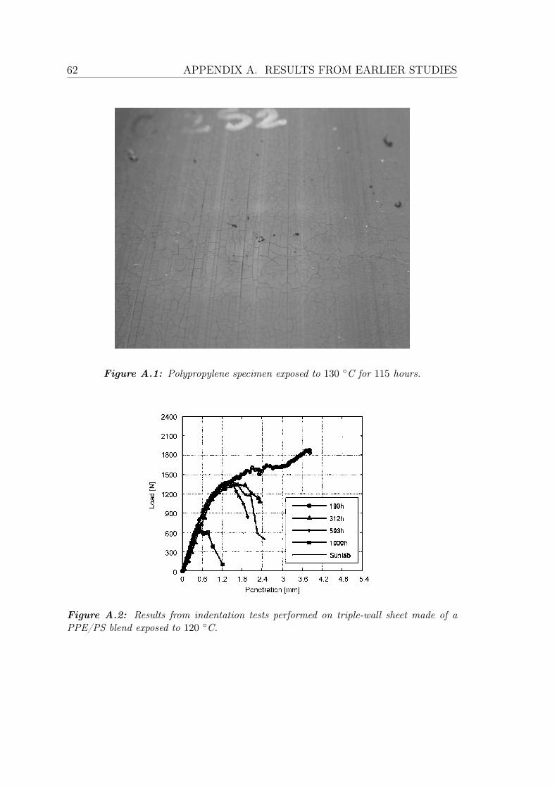
62 APPENDIX A. RESULTS FROM EARLIER STUDIES

20.03.2007 4

Fig. 10. APC-PP-G10 after 115 h at 130°C: No visible change/damage is observed on the surface.

Fig. 11. APC-PP-G25 after 115 h at 130°C: Visible changes/damage are observed on the surface; small surface "cracks".

Figure A.1: Polypropylene specimen exposed to 130 ◦C for 115 hours.

absorber can reach maximum temperatures of 145 1C [12],however in operative conditions stagnation is present in theabsorber for short periods of time when the water flow ofthe system is interrupted.

Several results as the ones shown in Fig. 15 indicate asignificant effect of the temperature and the exposure timeon the load–penetration curves. As a general conclusion,for a constant temperature, longer exposure times lead to areduction of the maximum indentation load that thespecimen can withstand during the test.

A mathematical model for different temperature/timeconditions may be used to predict how long time it will taketo reduce the maximum indentation load to a levelconsidered critical for the absorber operation. Using thismodel and the absorber temperature profile for one year ofoperation as a base for the temperature/time conditionsduring service life, it is possible to calculate after how mayyears the absorber will reach a level of degradation criticalfor its operation. Further details about the methods forestimation of the absorber service life will be discussed in asecond paper [18].

Short exposure times at high temperatures mainly affectthe plastic region of the curves. The typical failure observedin these cases is a permanent deflection on the surface and afracture in the specimen’s internal walls, as seen in Fig. 16.This kind of failure is typically represented as a gradualreduction of the slope in the plastic region of theload–penetration curves (Fig. 15) (312 h). The results areconsistent with the observation of severe reduction in theload at break after thermal exposure shown stress/strainmeasurements by Kahlen et al. [19].

If the exposure time is sufficiently long, the typicalfailure observed on the specimen is a break in the surfacewith almost no deformation on the specimen’s internalwalls (Fig. 17). In the load–penetration curve, this is

represented as a sharp break in the curve’s continuity in theviscoelastic region (Fig. 15) (1000 h).The failures shown in Figs. 16 and 17 suggest a change in

the properties of the material as consequence of thethermal degradation. These results show that the reductionof the ductility of the polymer leads to a brittle sheet.The reduction of the material’s ductility also occurs

under operational conditions as the Sunlab specimen inFig. 15 reveals. However, due to the cycles of low and hightemperature much longer exposition times are required toachieve the same level of degradation.

7. Results and conclusions

The mechanical integrity of the polymeric absorber hasbeen identified as a significant factor to determine its

ARTICLE IN PRESS

Fig. 15. Different times of exposure to 120 1C compared with a specimen

from a collector exposed to 208 days of outdoor weather condition (Oslo

climate).

Fig. 16. Typical failure in the plastic region of the load–penetration depth

curve.

Fig. 17. Typical failure in the viscoelastic region of the load–penetration

depth curve.

A. Olivares et al. / Solar Energy Materials & Solar Cells 92 (2008) 445–452 451

Figure A.2: Results from indentation tests performed on triple-wall sheet made of aPPE/PS blend exposed to 120 ◦C.

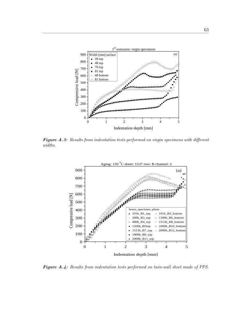
63

39

results are shown in Figure 6.17. The dimensions of the contact area of the indenter for

specimens with a width of 81 mm, 70 mm and 40 mm, are shown in Figure 6.18.

0 1 2 3 4 50

100

200

300

400

500

600

700

800

900

1st

extrusion: virgin specimens

Width [mm] surface

28 top

48 top

70 top

81 top

48 bottom

81 bottomC

om

pre

ssiv

e lo

ad [

N]

Indentation depth [mm]

(a)

0 1 2 3 4 50

100

200

300

400

500

600

700

800

900

2nd

extrusion: virgin specimens

Width [mm] surface

40 top

40 bottom

70 bottom

Co

mp

ress

ive

load

[N

]


(b)

Figure 6.17 Typical indentations curves for virgin specimens from the 1st (a) and 2

nd (b) extrusions sheets with

different widths of the specimens, for indenter oriented ║ to the inner walls of the specimens.

Figure 6.18 Dimensions of the contact area and non-contact area for specimens with a width of 81mm (left),

with a width of 70 mm (middle) and a width of 40 mm (right) where the last one does not have non-indenter

area.

Figure 6.17 displays the indentation curves for different widths of virgin specimens

from the 1st extrusion (a) and 2

nd extrusion (b) sheets, on the top and bottom surfaces of the

specimens. The curves obtained for specimens with a width of 70 mm and 81 mm show

similar shape. In these cases the curves have a double yield point. The 2nd

yield point for

specimens with a width of 81 mm has higher compressive load (790 N) than the specimens

with a width of 70 mm (630 N). The indentation depth where the 2nd

yield point occurs is

different as well, 3 mm and 3.5 mm for specimens with a width of 70 mm and 81 mm,

respectively. This difference in the values for the 2nd

yield point is because when the

specimens have a width bigger than the length of the indenter, the contact area is the first to

be deformed and then the non-contact area (longer the non-contact area higher compressive

load needed to deform the surface along the channel. Thus the force is not distributed

Figure A.3: Results from indentation tests performed on virgin specimens with differentwidths.

49

A.3 Thermal Treatment at 150 °C- first extrusion

A.3.1 Indenter parallel to the inner channels

0 1 2 3 4 5

0

100

200

300

400

500

600

700

800

900

Aging: 150 oC sheet: 1537 row: B channel: 2

hours_specimen_plane

101h_B1_top 101h_B2_bottom



1200h_B5top 1800h_B10_bottom


1800h_B9_top

2000h_B11_top

Com

pres

sive

load

[N

]


(a)

0 1 2 3 4 50

100

200

300

400

500

600

700

800

900

Aging: 150 oC sheet: 1537 row: C channel: 2


101h_C1_top 101h_C2_bottom




1513h_C7_top

1800h_C9_top

2000h_C11_top

Co

mp

ress

ive l

oad

[N

]


(b)

A.3 Compressive load vs indentation depth curves for the 1st extrusion exposed to 150 °C for different exposure

times for both surfaces of the specimens. Indentation tests performed with the indenter oriented ║ to the inner

walls of the specimens. In (a) tested the column B and in (b) tested the column C, both in the channel 2.

A.4 Thermal Treatment at 200 °C - First and second extrusion

A.4.1 Indenter parallel to the inner channels

First Extrusion

0 1 2 3 4 50

100

200

300

400

500

600

700

800

900 (a)

Aging: 200 oC sheet: 1509 column: B channel: 2



50h_B3_top 50h_B12_bottom*


211h_B7_top

*sheet 1539

Co

mp

ress

ive l

oad

[N

]


0 1 2 3 4 50

100

200

300

400

500

600

700

800

900 (b)

Aging: 200 oC sheet: 1509 column: C channel: 2



50h_C3_top 50h_C12_bottom*


*sheet 1539

Co

mp

ress

ive l

oad

[N

]


A.4 Compressive load vs indentation depth curves for the 1st extrusion exposed to 200 °C for different exposure

times for both surfaces of the specimens. Indentation tests performed with the indenter oriented ║ to the inner


Second Extrusion

0 1 2 3 4 50

100

200

300

400

500

600

700

800

900 (a)

Aging: 200 oC sheet: 1504 column: B channel 2

hours_specimen_side

20h_B1N_top 20h_B2N_bottom

50h_B3N_top 50h_B2N_bottom*

100h_B5N_top

211h_B7N_top

*sheet 1320

Co

mp

ress

ive l

oad

[N

]


0 1 2 3 4 50

100

200

300

400

500

600

700

800

900(b)

Aging: 200 oC sheet: 1504 column: C channel: 2

hours_specimen_side

20h_C1N_top 20h_C2N_bottom

50h_C3N_top 50h_C2N_bottom*

100h_C5N_top 100h_C6N_bottom

211h_C7N_top

*sheet 1320

Co

mp

ress

ive l

oad

[N

]


A.5 Compressive load vs indentation depth curves for the 2nd

extrusion exposed to 200 °C for different exposure

times for both palnes of the specimens. Indentation tests performed with the indenter oriented ║ to the inner


Figure A.4: Results from indentation tests performed on twin-wall sheet made of PPS.

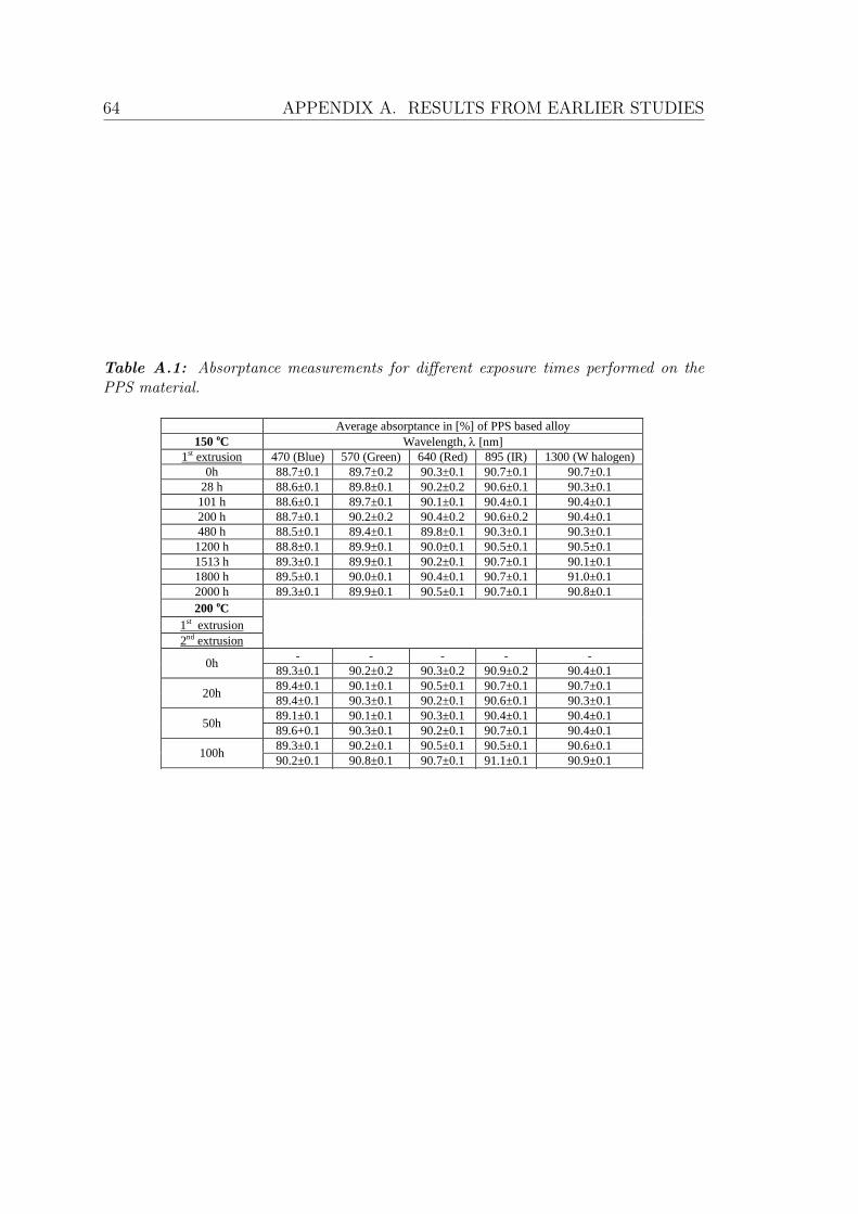
64 APPENDIX A. RESULTS FROM EARLIER STUDIES

Table A.1: Absorptance measurements for different exposure times performed on thePPS material.

25

Table 6.1 Average absorptance of the specimens measured in [%] for the 1st and 2

nd extrusions for different

wavelengths and the respective standard error. The specimens were exposed to heat load during different

periods at 150 ºC and 200 °C for the 1

st extrusion and 200

ºC for the 2

nd extrusion.

Average absorptance in [%] of PPS based alloy

150 oC Wavelength, [nm]

1st extrusion 470 (Blue) 570 (Green) 640 (Red) 895 (IR) 1300 (W halogen)

0h 88.7±0.1 89.7±0.2 90.3±0.1 90.7±0.1 90.7±0.1

28 h 88.6±0.1 89.8±0.1 90.2±0.2 90.6±0.1 90.3±0.1

101 h 88.6±0.1 89.7±0.1 90.1±0.1 90.4±0.1 90.4±0.1

200 h 88.7±0.1 90.2±0.2 90.4±0.2 90.6±0.2 90.4±0.1

480 h 88.5±0.1 89.4±0.1 89.8±0.1 90.3±0.1 90.3±0.1

1200 h 88.8±0.1 89.9±0.1 90.0±0.1 90.5±0.1 90.5±0.1

1513 h 89.3±0.1 89.9±0.1 90.2±0.1 90.7±0.1 90.1±0.1

1800 h 89.5±0.1 90.0±0.1 90.4±0.1 90.7±0.1 91.0±0.1

2000 h 89.3±0.1 89.9±0.1 90.5±0.1 90.7±0.1 90.8±0.1

200 oC

1st extrusion

2nd extrusion

0h - - - - -

89.3±0.1 90.2±0.2 90.3±0.2 90.9±0.2 90.4±0.1

20h 89.4±0.1 90.1±0.1 90.5±0.1 90.7±0.1 90.7±0.1

89.4±0.1 90.3±0.1 90.2±0.1 90.6±0.1 90.3±0.1

50h 89.1±0.1 90.1±0.1 90.3±0.1 90.4±0.1 90.4±0.1

89.6+0.1 90.3±0.1 90.2±0.1 90.7±0.1 90.4±0.1

100h 89.3±0.1 90.2±0.1 90.5±0.1 90.5±0.1 90.6±0.1

90.2±0.1 90.8±0.1 90.7±0.1 91.1±0.1 90.9±0.1

selective surface 78.9±0.1 86.8±0.1 93.0±0.1 97.3±0.1 86.1±0.2

Table 6.1 shows the average absorptance in percentage for virgin and exposed time

heated load specimens for both extrusions of the absorber sheets. In general, the absorptance

increases slightly with the wavelengths. This means that the black sheets reflect more in the

blue and less in the infrared. The results for specimens heated during different exposure times

shows there no significant variations of the absorptance.

The selective coated surface has higher reflectance in blue and less in infrared, thus

the absorptance is lower for blue and higher for infrared.

6.2 Emittance

The average emittance percentage values are presented in the Table 6.2.

Table 6.2 Results of the average emittance for different specimens from the 1st extrusion sheets.

specimen Nº of measurements Average Emittance in [%]

of PPS based alloy

Virgin-sheet 1537 23 70.7±0.9

Heated during 28 h 33 73.3±0.9

Selective surface 12 18.0±0.4

The results show that the non-selective surfaces have higher emmitance than for the

selective surface.

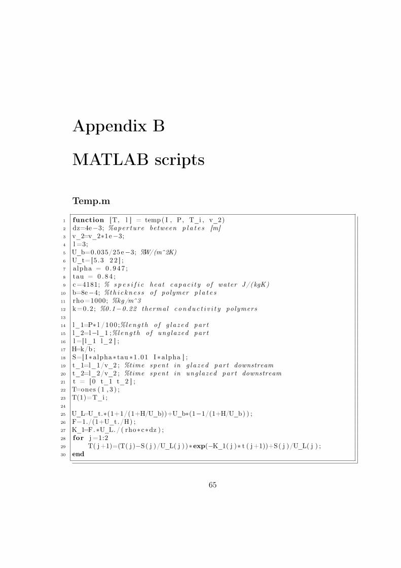
Appendix B

MATLAB scripts

Temp.m

1 function [T, l ] = temp( I , P, T_i , v_2)2 dz=4e−3; %aper ture between p l a t e s [m]3 v_2=v_2∗1e−3;4 l =3;5 U_b=0.035/25e−3; %W/(m^2K)6 U_t=[5.3 2 2 ] ;7 alpha = 0 . 9 4 7 ;8 tau = 0 . 8 4 ;9 c=4181; % s p e s i f i c heat capac i t y o f water J/(kgK)

10 b=8e−4; %th i c kn e s s o f polymer p l a t e s11 rho=1000; %kg/m^312 k=0.2; %0.1−0.22 thermal c ondu c t i v i t y polymers13

14 l_1=P∗ l /100 ;%leng t h o f g l a z ed par t15 l_2=l−l_1 ;%leng t h o f ung lazed par t16 l =[ l_1 l_2 ] ;17 H=k/b ;18 S=[ I ∗ alpha ∗ tau ∗1 .01 I ∗ alpha ] ;19 t_1=l_1/v_2 ; %time spent in g l a z ed par t downstream20 t_2=l_2/v_2 ; %time spent in ung lazed par t downstream21 t = [ 0 t_1 t_2 ] ;22 T=ones ( 1 , 3 ) ;23 T(1)=T_i ;24

25 U_L=U_t.∗(1+1/(1+H/U_b))+U_b∗(1−1/(1+H/U_b) ) ;26 F=1./(1+U_t. /H) ;27 K_1=F.∗U_L. / ( rho∗c∗dz ) ;28 for j =1:229 T( j+1)=(T( j )−S( j )/U_L( j ) )∗exp(−K_1( j )∗ t ( j +1))+S( j )/U_L( j ) ;30 end

65

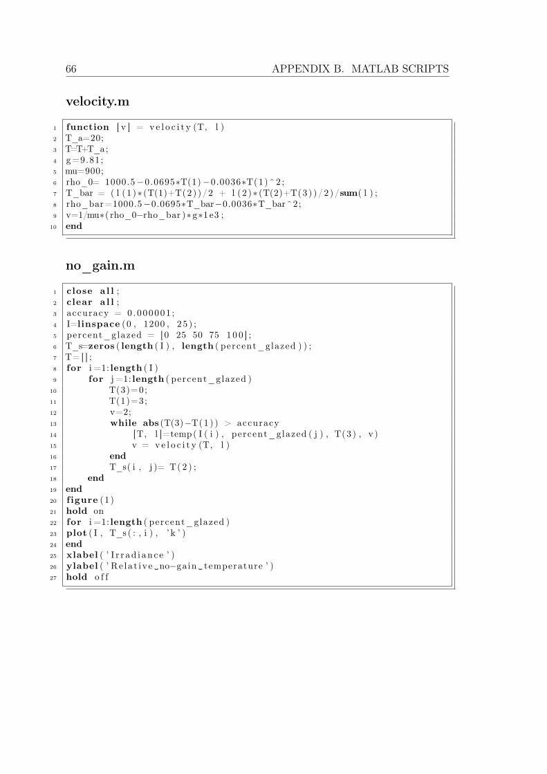
66 APPENDIX B. MATLAB SCRIPTS

velocity.m

1 function [ v ] = v e l o c i t y (T, l )2 T_a=20;3 T=T+T_a;4 g=9.81;5 mu=900;6 rho_0= 1000.5−0.0695∗T(1)−0.0036∗T(1)^2 ;7 T_bar = ( l ( 1 )∗ (T(1)+T(2) )/2 + l ( 2 )∗ (T(2)+T(3 ) ) /2 )/sum( l ) ;8 rho_bar=1000.5−0.0695∗T_bar−0.0036∗T_bar^2;9 v=1/mu∗( rho_0−rho_bar )∗ g∗1 e3 ;

10 end

no_gain.m

1 close a l l ;2 clear a l l ;3 accuracy = 0 .000001 ;4 I=linspace (0 , 1200 , 2 5 ) ;5 percent_glazed = [0 25 50 75 1 0 0 ] ;6 T_s=zeros ( length ( I ) , length ( percent_glazed ) ) ;7 T= [ ] ;8 for i =1: length ( I )9 for j =1: length ( percent_glazed )

10 T(3)=0;11 T(1)=3;12 v=2;13 while abs (T(3)−T(1 ) ) > accuracy14 [T, l ]=temp( I ( i ) , percent_glazed ( j ) , T(3 ) , v )15 v = v e l o c i t y (T, l )16 end17 T_s( i , j )= T( 2 ) ;18 end19 end20 f igure (1 )21 hold on22 for i =1: length ( percent_glazed )23 plot ( I , T_s ( : , i ) , ’ k ’ )24 end25 xlabel ( ’ I r r ad i an c e ’ )26 ylabel ( ’ Re l a t i v e ␣no−gain ␣ temperature ’ )27 hold o f f

67

efficiency.m

1 clear a l l ;2 close a l l ;3 accuracy = 0 .000001 ;4 l =3;5 dz=4e−3; %aper ture between p l a t e s [m]6 dx=1e−2;7 A=l ∗45∗dx ;8 T_a=20;9 T_i=linspace (−10 , 180 , 191 ) ;

10 c=4181;11 c ro s s_sec t i on = 45∗dx∗dz ;12 P=[0 25 50 75 1 0 0 ] ;13 l_1=P∗ l /100 ;%leng t h o f g l a z ed par t14 l_2=l−l_1 ;%leng t h o f ung lazed par t15 l =[ l_1 l_2 ] ;16 I =1000;17 c o l o r=’ rgckb ’ ;18 e f f=zeros ( length (P) , length (T_i ) ) ;19 temperature_out=zeros ( length (P) , length (T_i ) ) ;20 speed=zeros ( length (P) , length (T_i ) ) ;21 i t e r a t i v e=zeros ( length (P) , length (T_i ) ) ;22 barT=zeros ( length (P) , length (T_i ) ) ;23 marks=zeros (1 , length (P ) ) ;24 for i =1: length (P)25 for j =1: length (T_i)26 T=[0 0 0 ] ;27 v=1;28 dummy = T(3)+1;29 dummy_v=v ;30 while abs (dummy − T(3 ) ) > accuracy31 v=(dummy_v+v )/2 ;32 dummy_v=v ;33 dummy = T( 3 ) ;34 i t e r a t i v e ( i , j ) = i t e r a t i v e ( i , j ) + 1 ;35 [T, l ]=temp( I , P( i ) , T_i( j ) , v ) ;36 v=v e l o c i t y (T, l ) ;37 i f v<038 v=0;39 T(3)=T_i( j ) ;40 dummy = T( 3 ) ;41 end42

43 end44 e f f ( i , j )=(T(3)−T(1 ) )∗ v∗ c ro s s_sec t i on ∗c /( I ∗A) ;45 speed ( i , j ) = v ;46 barT ( i , j )=( l ( 1 )∗ (T(1)+T(2) )/2 + l ( 2 )∗ (T(2)+T(3 ) ) /2 )/sum( l ) ;47 temperature_out ( i , j )=T( 3 ) ;

68 APPENDIX B. MATLAB SCRIPTS

48 end49 end50 f igure (5 )51 box on52 axis ( [ 0 130 0 100 ] )53 xlabel ( ’Mean␣heat ␣ c a r r i e r ␣ temperature ␣above␣ambient␣ [^\ c i rcC ] ’ )54 ylabel ( ’ E f f i c i e n c y ␣ [%] ’ )55 hold on56 for i =1: length (P)57 Ef f=e f f ( i , : ) ;58 Ef f ( Eff <=0)=[];59 BarT=barT ( i , 1 : length ( E f f ) ) ;60 p=polyf it (BarT , Eff , 1 ) ;61 marks ( i )=−p (2)/p ( 1 ) ;62 x=linspace (0 , 130 , 100 ) ;63 plot (x , 100 .∗ ( p ( 1 ) . ∗ x+p ( 2 ) ) , ’ k ’ )64 p = polyf it ( temperature_out ( i , 1 : length ( E f f ) ) , Eff , 1 ) ;65 x=linspace (10 , 50 , 5 ) ;66 E=p ( 1 ) . ∗ x+p (2)67 end68 marks=round(marks ) ;69 f igure (1 )70 hold on71 f igure (2 )72 hold on73 for i =1: length (P) %Produces temp r i s e and v e l o c i t y74 V=speed ( i , : ) ; %as func t i on s o f i n l e t temp .75 V(V==0)=[];76 X=length (V)+1;77 f igure (1 )78 plot (T_i ( 1 :X) , [V 0 ] , ’ k ’ ) ;79 f igure (2 )80 plot (T_i ( 1 :X−1) , temperature_out ( i , ( 1 :X−1))−T_i ( 1 :X−1) , ’ k ’ ) ;81 i f i==2 | | i==3 | | i==482 j=V(T_i==marks ( i ) ) ;83 f igure (1 )84 plot (marks ( i ) , j , ’ k∗ ’ )85 end86 end87 hold o f f

Appendix C

Indentation tests

Figures C.1-C.3 show the results from the indentation tests on virgin specimens,specimens exposed to 140 ◦C for 1488 h and specimens exposed to 150 ◦C for 864h.

−1 0 1 2 3 4 5 6−500

0

500

1000

1500

2000

2500

3000



(a) Specimen from section A

−1 0 1 2 3 4 5 6−500

0

500

1000

1500

2000

2500



(b) Specimen from section B

Figure C.1: Results from indentation test for virgin specimens.

69

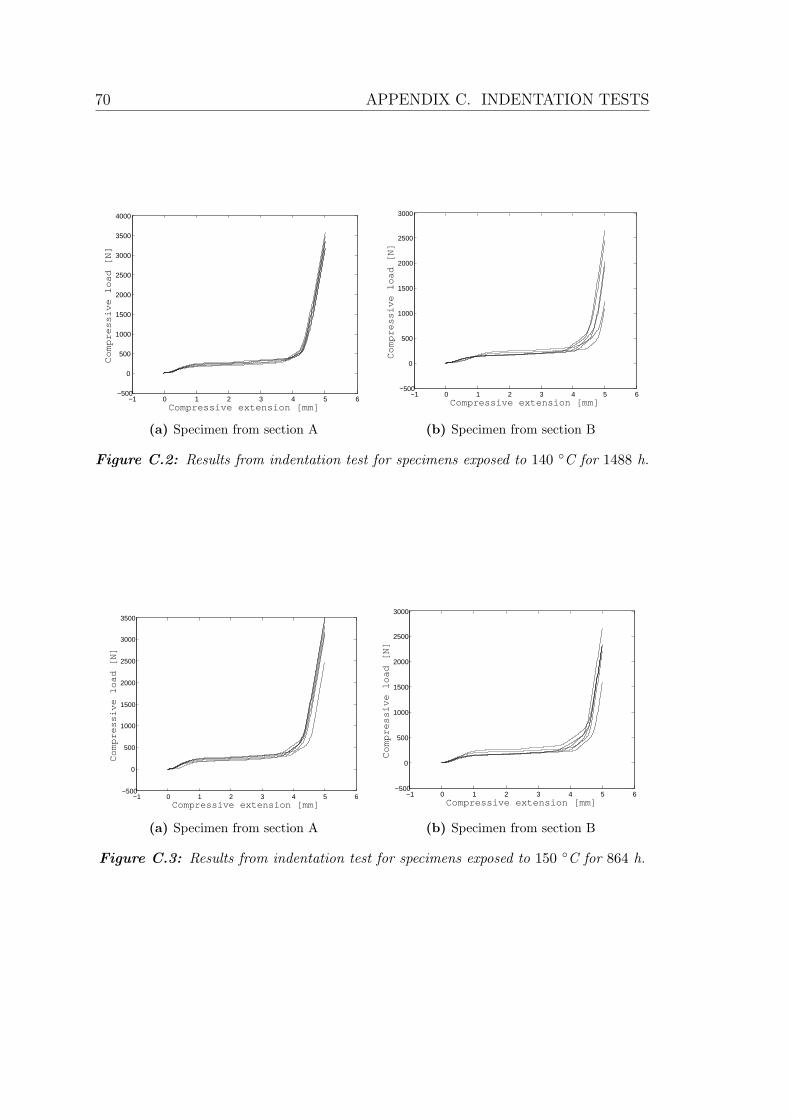
70 APPENDIX C. INDENTATION TESTS

−1 0 1 2 3 4 5 6−500

0

500

1000

1500

2000

2500

3000

3500

4000




−1 0 1 2 3 4 5 6−500

0

500

1000

1500

2000

2500

3000




Figure C.2: Results from indentation test for specimens exposed to 140 ◦C for 1488 h.

−1 0 1 2 3 4 5 6−500

0

500

1000

1500

2000

2500

3000

3500




−1 0 1 2 3 4 5 6−500

0

500

1000

1500

2000

2500

3000




Figure C.3: Results from indentation test for specimens exposed to 150 ◦C for 864 h.

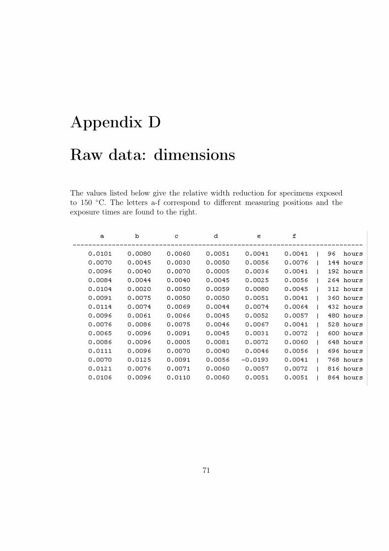
Appendix D

Raw data: dimensions

The values listed below give the relative width reduction for specimens exposedto 150 ◦C. The letters a-f correspond to different measuring positions and theexposure times are found to the right.

71

72 APPENDIX D. RAW DATA: DIMENSIONS

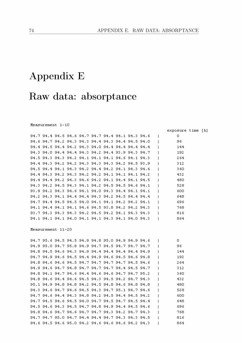
74 APPENDIX E. RAW DATA: ABSORPTANCE

Appendix E

Raw data: absorptance

natural circulating flat plate collectors - uio - duo

Documents