multilayer saint-venant equations over movable beds

Manuscript submitted to Website: http://AIMsciences.orgAIMS’ JournalsVolume X, Number 0X, XX 200X pp. X–XX

MULTILAYER SAINT-VENANT EQUATIONSOVER MOVABLE BEDS

Emmanuel Audusse and Fayssal Benkhaldoun

LAGA, Universite Paris 13, 99 Av J.B. Clement,93430 Villetaneuse, France

Jacques Sainte-Marie

Laboratoire d’Hydraulique Saint-Venant, 6 Quai Watier, BP 4978401 Chatou, France

Mohammed Seaid

School of Engineering and Computing Sciences, University of Durham,South Road, Durham DH1 3LE, UK

(Communicated by the associate editor name)

Abstract. We introduce a multilayer model to solve three-dimensional sedi-ment transport by wind-driven shallow water flows. The proposed multilayermodel avoids the expensive Navier-Stokes equations and captures stratifiedhorizontal flow velocities. Forcing terms are included in the system to modelmomentum exchanges between the considered layers. The topography frictionsare included in the bottom layer and the wind shear stresses are acting on thetop layer. To model the bedload transport we consider an Exner equation formorphological evolution accounting for the velocity field on the bottom layer.The coupled equations form a system of conservation laws with source terms.As a numerical solver, we apply a kinetic scheme using the finite volume dis-cretization. Preliminary numerical results are presented to demonstrate theperformance of the proposed multilayer model and to confirm its capabilityto provide efficient simulations for sediment transport by wind-driven shallowwater flows. Comparison between results obtained using the multilayer modeland those obtained using the single-layer model are also presented.

1. Introduction. The main concern of morphodynamics is to determine the evo-lution of bed levels for hydrodynamic systems such as rivers, estuaries, bays andother nearshore regions where water flows interact with the bed geometry. Exampleof applications include among others, beach profile changes due to severe wave cli-mates, seabed response to dredging procedures or imposed structures, and harboursiltation. The ability to design numerical methods able to predict the morphody-namic evolution of the coastal seabed has a clear mathematical and engineeringrelevance. The process of sediment transport is determined by the characteristicsof the hydraulic flow and sediment properties of the topography. Thus, dynamicsof the water and dynamics of the sediment must be studied using a mathematical

2000 Mathematics Subject Classification. Primary: 58F15, 58F17; Secondary: 53C35.Key words and phrases. Multilayer model, Saint-Venant equations, Sediment transport, Kinetic

schemes.The first author is supported by NSF grant xx-xxxx.

1

2 E. AUDUSSE, F. BENKHALDOUN, J. SAINTE-MARIE AND M. SEAID

model made of two different but dependent model variables: (i) a hydrodynamicvariable defining the dynamics of the water flow, and (ii) a bedload variable definingthe transport of sediments. In practice, morphodynamic problems involve couplingbetween a hydrodynamic model, which provides a description of the flow field lead-ing to a specification of local sediment transport rates, and an equation for bedlevel change which expresses the conservative balance of sediment volume and itscontinual redistribution with time. In the current study, the hydrodynamic modelis described by a multilayer Saint-Venant system proposed recently in [3] and thesediment transport is modelled by the well-established Exner equation [11]. Thecoupled equations form a system of conservation laws with source terms.

Morphodynamic coupling between classical single-layer Saint-Venant system andthe Exner equation has been extensively studied during the recent years, see forinstance [4, 6] and further references are therein. This coupled single-layer modelhas been widely used to model simple sediment transport problems in both one andtwo space dimensions and it has shown its ability to capture the correct hydraulicand sediment dynamics for open channel flows. However, in closed flow system, thissystem fails to capture the correct velocity fields and therefore, the correct sedimentfeatures. Indeed, for water flows in closed domains and subject to wind effects suchas water flows in coastal engineering, recirculation zones occur within the flow dy-namics. It is impossible to capture these recirculation features using the single-layermodel since by construction, the single-layer Saint-Venant system does not accountfor vertical effects. In order to overcome this drawback, we propose in the presentstudy, a coupling between the multilayer Saint-Venant system and the Exner equa-tion. The main advantage of the multilayer approach lies in the possibility to obtaina detailed description of the velocity in the flow while keeping a relative simplicityand a great robustness in the numerical procedure. On one hand, as opposed to whathappens for classical single-layer model, the multilayer approach allows for consid-ering quite complex flows as wind driven circulation in closed basins such as coastalregions, lake or estuary among others. On the other hand, as opposed to whathappens for the three dimensional incompressible hydrostatic free surface Navier-Stokes equations widely used in the oceanographic community, the multilayer modelallows for considering a simplified two-dimensional problem in fixed domains. Themultilayer Saint-Venant system that we consider here has some relations with otherNavier-Stokes integrated models [10, 14] but its structure is fundamentally differentsince it is essentially a two-dimensional problem. The proposed multilayer modelalso differs from other multilayer models recently introduced in [8, 18, 5] since thesemodels consider non-miscible fluids with different densities. We refer the reader to[3] for numerical evidences of the ability of the proposed multilayer Saint-Venantmodel to reproduce environmental flows on fixed beds. The aim of this paper isto investigate the performance of this multilayer model to approximate numericalsolutions of the shallow water flows over movable beds. To our best knowledge, thisis the first time that numerical results for coupled multilayer Saint-Venant systemand Exner equation are presented.

In this paper, first the governing equations for the morphodynamic problems areformulated. Thereafter, the solution procedure employed to solve the morphody-namic problems is presented. After experiments with the different approaches fora morphodynamic example, results obtained for single-layer and multilayer modelsare discussed. Concluding remarks end the paper.

MULTILAYER SAINT-VENANT EQUATIONS OVER MOVABLE BEDS 3

h

h

h

hM−1

M

2

1

u

u

1

2

B

Wind

uM

M−1u

H

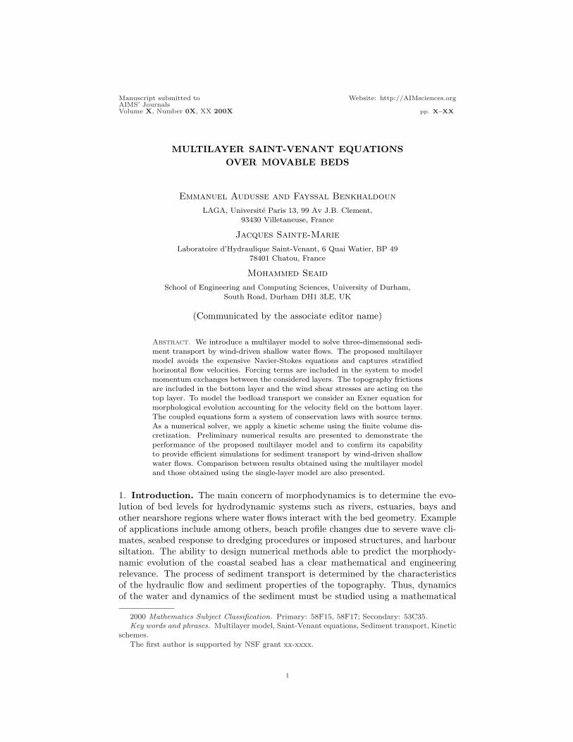
Figure 1. Schematic of a multilayer Saint-Venant system.

2. Governing Equations for Sediment Transport Problems. In this sectionwe describe the physical model used for modelling the sediment transport by wind-driven shallow water flows. Here, the Multilayer Saint-Venant equations are brieflyrecast for the hydrodynamics followed with a short description of the Exner equationfor the morphodynamics. In the present work, only bed load is considered in thiswork and the transport of suspended sediments is neglected.

2.1. Multilayer Saint-Venant Equations. The governing equations are obtainedstarting from the three-dimensional hydrostatic incompressible Navier-Stokes equa-tions with free surface by considering a vertical P0 type discretization of the hori-zontal velocity. This vertical discretization defines some layers in the flow and theequations are vertically integrated on each layer separately. In the simplest caseof the Euler equations with a flat bottom, this procedure leads to the followingequations for each layer α

∂hα

∂t+

∂hαuα

∂x= Gα+1/2 −Gα−1/2, (1)

∂hαuα

∂t+

∂

∂x

(hαu2

α

)+ ghα

∂H

∂x= uα+1/2Gα+1/2 − uα−1/2Gα−1/2, (2)

where hα(t, x) is the height of the αth layer, uα(t, x) is the local water velocity for theαth layer and g the gravitational acceleration, compare Figure 1 for an illustration.In the right-hand side of the above equations, Gα+1/2 denotes a mass exchangeterm and uα+1/2 the interface velocity between neighbouring layers. A global massequation for the whole flow is obtained by adding all the layer mass equations (1). Itis coupled with M momentum equations (2), one for each of the M layers introducedin the vertical discretization. We refer to [3] for a detailed derivation of the modelwhen Navier-Stokes equations are considered. It should be pointed out that thelayers defined in the model do not refer to physical interfaces between non-misciblefluids but to a meshless discretization of the flow domain. Hence, the possibility ofwater exchange between the layers is accounted for in the model. The great interestof this strategy is to preserve an accurate description of the velocity profile but to


deal with a two-dimensional fluid model and thus to avoid the difficult drawback ofmeshing a three-dimensional moving domain for which the free-surface may presentvery sharp profiles such as dam break problems and hydraulic jumps. In the currentstudy, for simplicity in the presentation, we consider the one-dimensional version ofthe model. Thus, the equations of the multilayer Saint-Venant system are given by

∂h

∂t+

M∑

λ=1

λα∂ (huα)

∂x= 0,

(3)∂ (huα)

∂t+

∂

∂x

(hu2

α + hpα

)= Fα, α = 1, 2, . . . , M,

where h(t, x) now denotes the water height of the whole flow system and λα denotesthe relative size of the αth layer with

M∑α=1

λα = 1.

The pressure term pα is defined as

pα =12ghα + pα+1/2, pα+1/2 =

M∑

β=α+1

ghβ .

The source term Fα is the external force acting on the layer α and accounting forthe friction and momentum exchange effects. Thus,

Fα = Fu + Fp + Fb + Fw + Fµ, α = 1, 2, . . . , M, (4)

where the two first terms Fu and Fp are related to the momentum exchanges be-tween the layers that are defined through the vertical P0 discretization of the flow.The forcing term Fu is related to advection process whereas the term Fp takes intoaccount for pressure effects. The three last terms Fb, Fw and Fµ are related tofriction effects. The bed friction forcing term Fb is acting only on the lower layerand the wind-driven forcing term Fw is acting only on the upper layer. The internalfriction term Fµ models the friction between neighbouring layers.

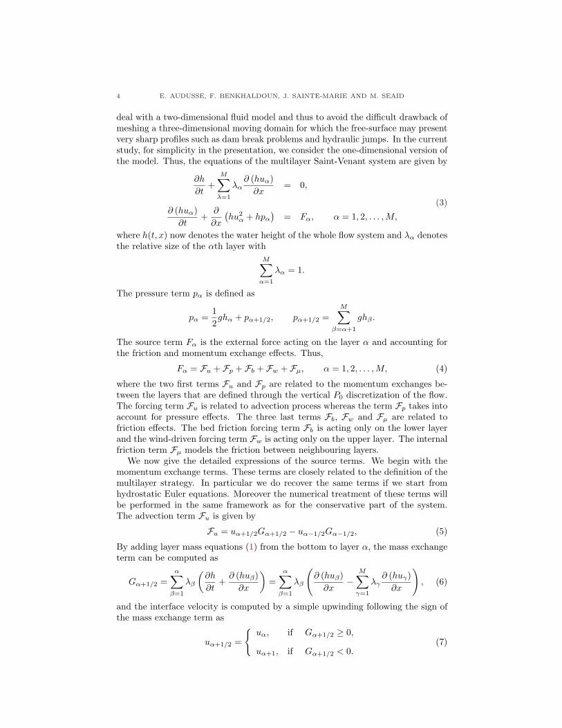
We now give the detailed expressions of the source terms. We begin with themomentum exchange terms. These terms are closely related to the definition of themultilayer strategy. In particular we do recover the same terms if we start fromhydrostatic Euler equations. Moreover the numerical treatment of these terms willbe performed in the same framework as for the conservative part of the system.The advection term Fu is given by

Fu = uα+1/2Gα+1/2 − uα−1/2Gα−1/2, (5)

By adding layer mass equations (1) from the bottom to layer α, the mass exchangeterm can be computed as

Gα+1/2 =α∑

β=1

λβ

(∂h

∂t+

∂ (huβ)∂x

)=

α∑

β=1

λβ

(∂ (huβ)

∂x−

M∑γ=1

λγ∂ (huγ)

∂x

), (6)

and the interface velocity is computed by a simple upwinding following the sign ofthe mass exchange term as

uα+1/2 =

{uα, if Gα+1/2 ≥ 0,

uα+1, if Gα+1/2 < 0.(7)


B

Wind

Hu

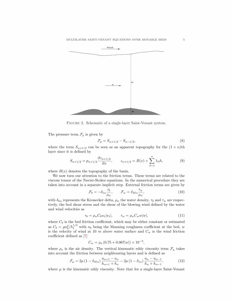
Figure 2. Schematic of a single-layer Saint-Venant system.

The pressure term Fp is given by

Fp = Sα+1/2 − Sα−1/2, (8)

where the term Sα+1/2 can be seen as an apparent topography for the (1 + α)thlayer since it is defined by

Sα+1/2 = pα+1/2

∂zα+1/2

∂x, zα+1/2 = B(x) +

α∑

β=1

λβh, (9)

where B(x) denotes the topography of the basin.We now turn our attention to the friction terms. These terms are related to the

viscous tensor of the Navier-Stokes equations. In the numerical procedure they aretaken into account in a separate implicit step. External friction terms are given by

Fb = −δ1ατb

ρw, Fw = δMα

τw

ρw, (10)

with δkα represents the Kronecker delta, ρw the water density, τb and τw are respec-tively, the bed shear stress and the shear of the blowing wind defined by the waterand wind velocities as

τb = ρwCbu1|u1|, τw = ρwCww|w|, (11)

where Cb is the bed friction coefficient, which may be either constant or estimatedas Cb = gn2

b/h1/31 with nb being the Manning roughness coefficient at the bed, w

is the velocity of wind at 10 m above water surface and Cw is the wind frictioncoefficient defined as [7]

Cw = ρa (0.75 + 0.067|w|)× 10−3,

where ρa is the air density. The vertical kinematic eddy viscosity term Fµ takesinto account the friction between neighbouring layers and is defined as

Fµ = 2µ (1− δMα)uα+1 − uα

hα+1 + hα− 2µ (1− δ1α)

uα − uα−1

hα + hα−1, (12)

where µ is the kinematic eddy viscosity. Note that for a single-layer Saint-Venant


problem, the model (3) reduces to

∂H

∂t+

∂ (Hu)∂x

= 0,

(13)∂ (Hu)

∂t+

∂

∂x

(Hu2 +

12gH2

)= −gH

∂B

∂x− τb

ρw+

τw

ρw,

where H is still the water depth but u is now the water velocity of the whole flow,compare Figure 2 for an illustration.

2.2. Exner Equation. To update the bed-load in the multilayer system (3), weused the Exner equation given by

(1− p)∂B

∂t+

∂Q

∂x= 0, (14)

where p is the sediment porosity assumed to be constant and the sediment dischargeQ can be evaluated by the simple formula introduced in [11]

Q(u1) = Au1 |u1|m , (15)

with u1 is the velocity of the lower layer, m and A are coefficients usually obtainedfrom experiments taking into account the grain diameter and the kinematic viscosityof the sediment. In practice, the values of the coefficient A are between 0 and 1depending on the interaction between the sediment transport and the water flow.Another formula frequently used for the sediment discharge Q is given in [13]

Q(u1, h1) = 8√

g(s− 1)d350

(n2

bu21

(s− 1)d50h131

− 0.047

) 32

, (16)

where s = ρs

ρwis the grain specific gravity, with ρs the sediment density. Note

that most of existing formulations for sediment transport models are empirical todiffering extents and have been derived from experiments and measured data. Itshould be stressed that the method described in this paper can be applied to otherforms of sediment transport fluxes without major conceptual modifications. Forinstance, the bed-load sediment transport functions proposed in [16, 17] can alsobe handled by the proposed multilayer model. Notice that the parameters nb,d50, ρs, p and A appeared in above equations are user-defined constants in thesediment transport model. In practice, the selection of these coefficients are problemdependent and their discussion is postponed for section 4 where numerical exampleswill be presented. In the following we refer as the coupled multilayer system whenwe consider the solution h, uα, B of the system of the N + 2 equations (3) and(14) and we refer as the coupled single-layer system when we consider the solutionh, u, B of the system of three equations (13)-(14). We refer to [4, 6] for a detailedanalysis of the coupled single-layer system. The theoretical analysis of the coupledmultilayer system will be performed in a future work. We refer to [3] for an analysisof the multilayer system (3) when the bottom does not evolve in time.

3. Solution Procedure. In this section we describe the numerical method that isused to solve the coupled multilayer model. We first briefly recast the strategy thatis used to solve the coupled single-layer model. Let us notice that three strategiescan be used to deal with the numerical treatment of these coupled problems. Thefirst one is referred as the quasi-steady approach. The fluid model is first solvedon a fixed bottom until a steady state is reached. Then the bottom is updated by


using in the Exner equation (14) the stationary flow velocity that was computedin the fluid step and we start again with the fluid problem but with consideringthe new bottom profile. The interest of this method is to make independent thenumerical procedures that are used for the solution of fluid and bottom problems.The main drawbacks are the difficulty to estimate the right time step in the Exnerequation and the limitation to deal with transient flow as dam break problems. Asecond possible strategy is to solve each equation separately but at each time step.As for the first one, this strategy allows us to use different numerical procedures foreach equation but it avoids to estimate two different time steps. It also allows us towork with transient problems but it can introduce some numerical diffusion on thebottom topography. The third possibility is to consider a coupled problem whereall of the variables h, uα, B are updated at each time step using the same numericalprocedure. This third strategy requires development of a consistent algorithm whichsolves the multilayer aspects of the problem coupled to those offered by the Exnerequation. The development of such an algorithm is under consideration and resultswill be published in the future. In this paper, we adopt the third strategy for thesingle-layer coupled model and the second strategy is used for the solution of themultilayer system.

3.1. Solution procedure for the coupled single-layer model. For the coupledsingle-layer model, the equations (13) and (14) can be rearranged in a system ofconservation laws with a source term as

∂W∂t

+∂F(W)

∂x= S(W), (17)

where W contains the conservative variables

W =

H

Hu

B

, F(W) =

Hu

Hu2 +12gH2 + gHB

11− p

Q

,

S(W) =

0

gB∂H

∂x− τb

ρw+

τw

ρw

0

.

For smooth solutions the equations (13) and (14) can also be formulated (withouttaking into account the friction terms) as

∂U∂t

+∂G(U)

∂x= 0, (18)

where U contains the primitive variables

U =

H

u

B

, G(U) =

Hu12u2 + g(H + B)

11− p

Q

.

The eigenvalues µk (k = 1, 2, 3) associated with the Jacobian matrix in (18) are thezeros of the characteristic polynomial

P (µ) = µ3 − 2uµ2 +(u2 − g(H + d)

)µ + gud, (19)


with d = 1(1−p)Am|u|m−1. Thus, the eigenvalues of the Jacobian matrix are

µ1 = 2√−Z cos

(13θ

)+

23u,

µ2 = 2√−Z cos

(13(θ + 2π)

)+

23u, (20)

µ3 = 2√−Z cos

(13(θ + 4π)

)+

23u,

where θ = arcos(

R√−Z3

), with

Z = −19

(u2 + 3g(H + d)

), R =

u

54(9g(2H − d)− 2u2

).

Let us discretize the spatial domain into control volumes [xi−1/2, xi+1/2] with uni-form size ∆x = xi+1/2 − xi−1/2 and divide the temporal domain into subintervals[tn, tn+1] with uniform size ∆t. Following the standard finite volume formulation,we integrate the equation (17) with respect to time and space over the domain[tn, tn+1]× [xi−1/2, xi+1/2] to obtain the following discrete equation

Wn+1i = Wn

i −∆t

∆x

(F

(Wn

i+1/2

)− F

(Wn

i−1/2

))+ ∆tSn

i , (21)

where Wni is the time-space average of the solution W at time tn in the domain

[xi−1/2, xi+1/2] and F(Wni±1/2) is the numerical flux at x = xi±1/2 and time tn i.e.,

Wni =

1∆t∆x

∫ tn+1

tn

∫ xi+1/2

xi−1/2

W(t, x) dt dx.

The spatial discretization of the equation (21) is complete when a numerical con-struction of the fluxes F(Wn

i±1/2) is chosen. In the current study, the primitivevariables Un

i+1/2 are used to compute the averaged states in (21) as

Uni+1/2 =

12

(Un

i+1 + Uni

)− 12sgn

[B

(U

)] (Un

i+1 −Uni

), (22)

where the averaged state is calculated as

U =

Hi + Hi+1

2

ui

√Hi + ui+1

√Hi+1√

Hi +√

Hi+1

Bi + Bi+1

2

, (23)

and the sign matrix is given by

sgn[B

(U

)]= R (

U)sgn

[Λ

(U

)]R−1(U

), (24)

with sgn[Λ

(U

)]is a diagonal matrix that contains the signs of the eigenvalues µk

(20) calculated at the averaged state (23). The right and left eigenvector matrices


are given by

R (U

)=

1 1 1

β1

H

β2

H

β3

H

β2

1 − c2

c2

β2

2 − c2

c2

β2

3 − c2

c2

, (25)

R−1(U

)=

c2 + β2β3

µ12µ13

−h(β2 + β3)µ12µ13

c2

µ12µ13

c2 + β1β3

µ21µ23

−h(β1 + β3)µ21µ23

c2

µ21µ23

c2 + β1β2

µ31µ32

−h(β1 + β2)µ31µ32

c2

µ31µ32

, (26)

where c =√

gH is the wave speed and

βk = µk − u, µkj = µk − µj , k, j = 1, 2, 3.

Remark that, since the predictor stage in (22) uses the primitive variables Uni+1/2,

the source term appears only in the corrector stage. The source term approximationSn

i in the corrector stage is reconstructed such that the C-property is satisfied, see[4, 6] for the details.

3.2. Solution procedure for the coupled multilayer model. In [3] a numer-ical strategy is presented for the discretization of the multilayer system (3). Thisstrategy is mostly based on a kinetic interpretation of the model. Here we proposeto extend this approach to the coupled multilayer system formed by the equations(3) and (14). The kinetic formulation was first introduced for other fluid models[15, 1] but it is particularly interesting in the multilayer context since it is a wayto provide a stable numerical scheme without requiring the computation of the ei-genvalues of the (exact or approximated) Jacobian matrix. In the following we firstbriefly recall the kinetic interpretation of the fluid model and then we present a ki-netic interpretation of the Exner equation. Let us notice that the advection sourceterm Fu can be included in the kinetic interpretation and we use the relation (6) todiscretize it by using the kinetic fluxes. The apparent topographic source term Fp

and the friction source terms Fb, Fw and Fµ are not included in the kinetic inter-pretation. The apparent topographic source term can be handled out by the use ofan extension of the hydrostatic reconstruction procedure introduced in [2]. We usea simple implicit solver to deal with the friction source terms. This approach hasbeen proved to be efficient in the case of the classical Saint-Venant system [1, 2].

We introduce a kinetic velocity ξ and an even probability χ(ξ) with second mo-mentum equal to unity. For each layer α we define the kinetic function Mα as

Mα =hα(x, t)

cαχ

(ξ − uα(x, t)

cα

), c2

α =ghα

2. (27)


We claim that (h, uα) is a solution of the multilayer Saint-Venant model (3) if andonly if Mα is a solution of the kinetic equation

∂Mα

∂t+ ξ

∂Mα

∂x= Qα, (28)

where Qα is a kernel such that its two first integrals with respect to ξ vanish. Thecentral idea of the proof is the fact that the integration with respect to ξ of thekinetic equation (28) allows us to recover the momentum equation in (3) for thelayer α. The mass equation in (3) can be recovered by adding all the integrationwith respect to ξ of kinetic equations (28) for all layers. Note that the right-handside of multilayer system (3) is not included in this sketch of the proof. We refer thereader to [3] for a complete proof where the advection momentum exchange terms(5) are included in the kinetic formulation.

We now introduce a kinetic interpretation for the Exner equation (14). We definea new density function

Mb(ξ,B, u) = Bδ

(ξ − Q(u)

B

), (29)

where δ denotes the Dirac measure (which is a particular case of even probability)and we claim that (h, uα, B) is a solution of the coupled multilayer system formedby the equations (3) and (14) if and only if the family ({Mα},Mb) is solution of thesystem of following linear equations

∂Mα

∂t+ ξ

∂Mα

∂x= Qα,

(30)∂Mb

∂t+ ξ

∂Mb

∂x= Qb.

The equivalence between kinetic equation (29) and Exner equation (14) is also dueto the fact that we recover equation (14) by a simple integration with respect to ξof the equation (29). Note that the kinetic interpretation is very helpful to designa simple and stable finite volume scheme for the coupled multilayer system. Let usrecall the general form of an explicit finite volume scheme for this system

Un+1i = Un

i −∆t

∆x

(Fn

i+1/2 − Fni−1/2

),

with U = (H, Hu1, . . . , HuM , B)T , where subscripts i and M and superscript nrefer to the horizontal and vertical space discretization and time discretization,respectively. The definition of the numerical flux Fi+1/2 characterizes the chosenfinite volume method. In kinetic scheme this numerical flux is first designed atthe kinetic level for the linear system (30). The linear structure of the systemmakes the choice very natural and we simply apply an upwind scheme following thesign of the kinetic velocity ξ. Since the macroscopic system is obtained from thekinetic equations after a simple integration procedure, we can do the same thing forthe numerical scheme and we do recover a numerical scheme for the macroscopicsystem by considering a simple integration of the kinetic upwind scheme. Thisstrategy is quite powerful since it leads to a stable and simple numerical scheme.We should mention that by stability we mean that the numerical scheme preservessome physical properties such as the positivity of the water height and by simplicitywe mean that the kinetic interpretation does not explicitly appear in the numericalscheme since all the computations in the integration process can be performed


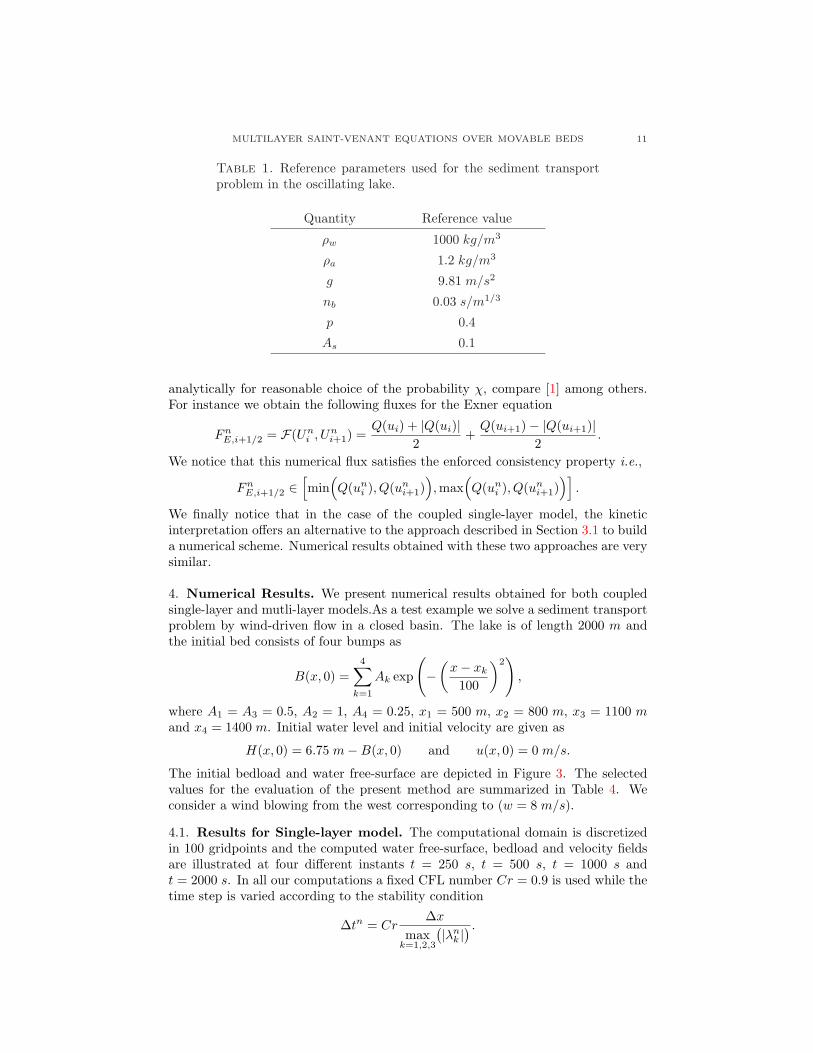
Table 1. Reference parameters used for the sediment transportproblem in the oscillating lake.

Quantity Reference value

ρw 1000 kg/m3

ρa 1.2 kg/m3

g 9.81 m/s2

nb 0.03 s/m1/3

p 0.4

As 0.1

analytically for reasonable choice of the probability χ, compare [1] among others.For instance we obtain the following fluxes for the Exner equation

FnE,i+1/2 = F(Un

i , Uni+1) =

Q(ui) + |Q(ui)|2

+Q(ui+1)− |Q(ui+1)|

2.

We notice that this numerical flux satisfies the enforced consistency property i.e.,

FnE,i+1/2 ∈

[min

(Q(un

i ), Q(uni+1)

),max

(Q(un

i ), Q(uni+1)

)].

We finally notice that in the case of the coupled single-layer model, the kineticinterpretation offers an alternative to the approach described in Section 3.1 to builda numerical scheme. Numerical results obtained with these two approaches are verysimilar.

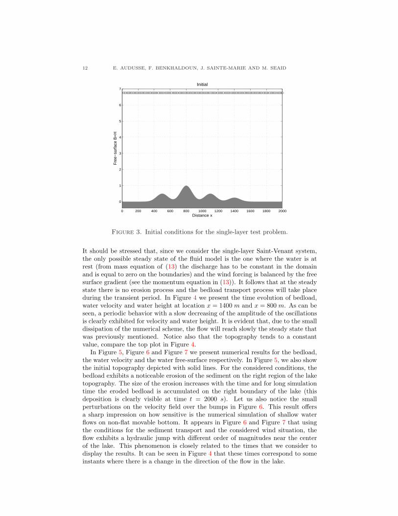
4. Numerical Results. We present numerical results obtained for both coupledsingle-layer and mutli-layer models.As a test example we solve a sediment transportproblem by wind-driven flow in a closed basin. The lake is of length 2000 m andthe initial bed consists of four bumps as

B(x, 0) =4∑

k=1

Ak exp

(−

(x− xk

100

)2)

,

where A1 = A3 = 0.5, A2 = 1, A4 = 0.25, x1 = 500 m, x2 = 800 m, x3 = 1100 mand x4 = 1400 m. Initial water level and initial velocity are given as

H(x, 0) = 6.75 m−B(x, 0) and u(x, 0) = 0 m/s.

The initial bedload and water free-surface are depicted in Figure 3. The selectedvalues for the evaluation of the present method are summarized in Table 4. Weconsider a wind blowing from the west corresponding to (w = 8 m/s).

4.1. Results for Single-layer model. The computational domain is discretizedin 100 gridpoints and the computed water free-surface, bedload and velocity fieldsare illustrated at four different instants t = 250 s, t = 500 s, t = 1000 s andt = 2000 s. In all our computations a fixed CFL number Cr = 0.9 is used while thetime step is varied according to the stability condition

∆tn = Cr∆x

maxk=1,2,3

(|λnk |

) .


0 200 400 600 800 1000 1200 1400 1600 1800 2000

0

1

2

3

4

5

6

7

Distance x

Free

−sur

face

B+H

Initial

Figure 3. Initial conditions for the single-layer test problem.

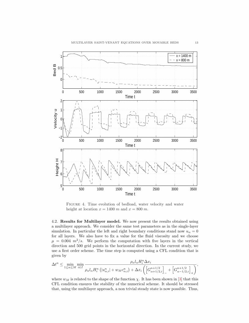
It should be stressed that, since we consider the single-layer Saint-Venant system,the only possible steady state of the fluid model is the one where the water is atrest (from mass equation of (13) the discharge has to be constant in the domainand is equal to zero on the boundaries) and the wind forcing is balanced by the freesurface gradient (see the momentum equation in (13)). It follows that at the steadystate there is no erosion process and the bedload transport process will take placeduring the transient period. In Figure 4 we present the time evolution of bedload,water velocity and water height at location x = 1400 m and x = 800 m. As can beseen, a periodic behavior with a slow decreasing of the amplitude of the oscillationsis clearly exhibited for velocity and water height. It is evident that, due to the smalldissipation of the numerical scheme, the flow will reach slowly the steady state thatwas previously mentioned. Notice also that the topography tends to a constantvalue, compare the top plot in Figure 4.

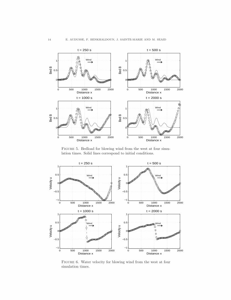
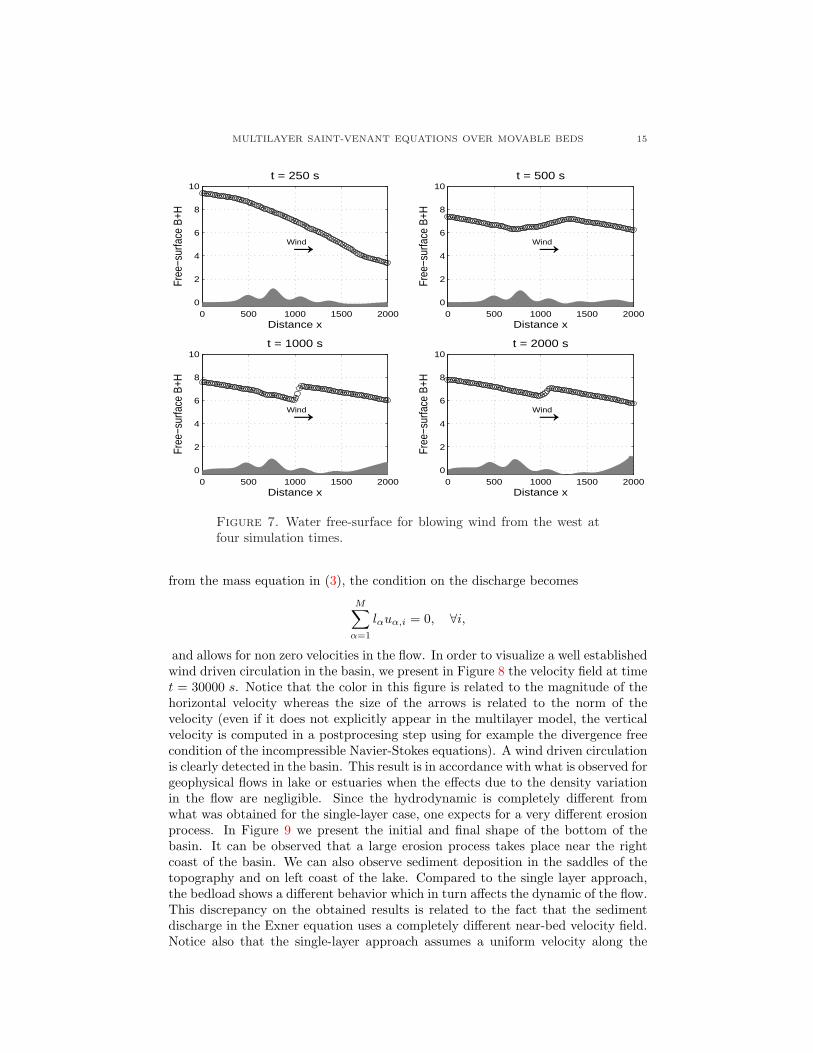
In Figure 5, Figure 6 and Figure 7 we present numerical results for the bedload,the water velocity and the water free-surface respectively. In Figure 5, we also showthe initial topography depicted with solid lines. For the considered conditions, thebedload exhibits a noticeable erosion of the sediment on the right region of the laketopography. The size of the erosion increases with the time and for long simulationtime the eroded bedload is accumulated on the right boundary of the lake (thisdeposition is clearly visible at time t = 2000 s). Let us also notice the smallperturbations on the velocity field over the bumps in Figure 6. This result offersa sharp impression on how sensitive is the numerical simulation of shallow waterflows on non-flat movable bottom. It appears in Figure 6 and Figure 7 that usingthe conditions for the sediment transport and the considered wind situation, theflow exhibits a hydraulic jump with different order of magnitudes near the centerof the lake. This phenomenon is closely related to the times that we consider todisplay the results. It can be seen in Figure 4 that these times correspond to someinstants where there is a change in the direction of the flow in the lake.


0 500 1000 1500 2000 2500 3000 3500

0

0.5

1

Time t

Be

d B

x = 1400 mx = 800 m

0 500 1000 1500 2000 2500 3000 3500−2

−1

0

1

2

Time t

Ve

locity u

0 500 1000 1500 2000 2500 3000 35005

6

7

8

Time t

He

igh

t H

Figure 4. Time evolution of bedload, water velocity and waterheight at location x = 1400 m and x = 800 m.

4.2. Results for Multilayer model. We now present the results obtained usinga multilayer approach. We consider the same test parameters as in the single-layersimulation. In particular the left and right boundary conditions stand now uα = 0for all layers. We also have to fix a value for the fluid viscosity and we chooseµ = 0.004 m2/s. We perform the computation with five layers in the verticaldirection and 500 grid points in the horizontal direction. In the current study, weuse a first order scheme. The time step is computed using a CFL condition that isgiven by

∆tn ≤ min1≤α≤M

mini∈I

ραlαHni ∆xi

ραlαHni

(|unα,i|+ wMcn

α,i

)+ ∆xi

([G

n+1/2α+1/2,i

]−

+[G

n+1/2α−1/2,i

]+

) ,

where wM is related to the shape of the function χ. It has been shown in [3] that thisCFL condition ensures the stability of the numerical scheme. It should be stressedthat, using the multilayer approach, a non trivial steady state is now possible. Thus,


0 500 1000 1500 2000

0

0.5

1

Distance x

Bed

B

→Wind

t = 250 s

0 500 1000 1500 2000

0

0.5

1

Distance x

Bed

B

→Wind

t = 500 s

0 500 1000 1500 2000

0

0.5

1

Distance x

Bed

B

→Wind

t = 1000 s

0 500 1000 1500 2000

0

0.5

1

Distance x

Bed

B

→Wind

t = 2000 s

Figure 5. Bedload for blowing wind from the west at four simu-lation times. Solid lines correspond to initial conditions.

0 500 1000 1500 2000−1

−0.5

0

0.5

1

Distance x

Velo

city

u →Wind

t = 250 s

0 500 1000 1500 2000−1

−0.5

0

0.5

1

Distance x

Velo

city

u →Wind

t = 500 s

0 500 1000 1500 2000−1

−0.5

0

0.5

1

Distance x

Velo

city

u →Wind

t = 1000 s

0 500 1000 1500 2000−1

−0.5

0

0.5

1

Distance x

Velo

city

u →Wind

t = 2000 s

Figure 6. Water velocity for blowing wind from the west at foursimulation times.


0 500 1000 1500 20000

2

4

6

8

10

Distance x

Free

−sur

face

B+H

→Wind

t = 250 s

0 500 1000 1500 20000

2

4

6

8

10

Distance x

Free

−sur

face

B+H

→Wind

t = 500 s

0 500 1000 1500 20000

2

4

6

8

10

Distance x

Free

−sur

face

B+H

→Wind

t = 1000 s

0 500 1000 1500 20000

2

4

6

8

10

Distance x

Free

−sur

face

B+H

→Wind

t = 2000 s

Figure 7. Water free-surface for blowing wind from the west atfour simulation times.

from the mass equation in (3), the condition on the discharge becomes

M∑α=1

lαuα,i = 0, ∀i,

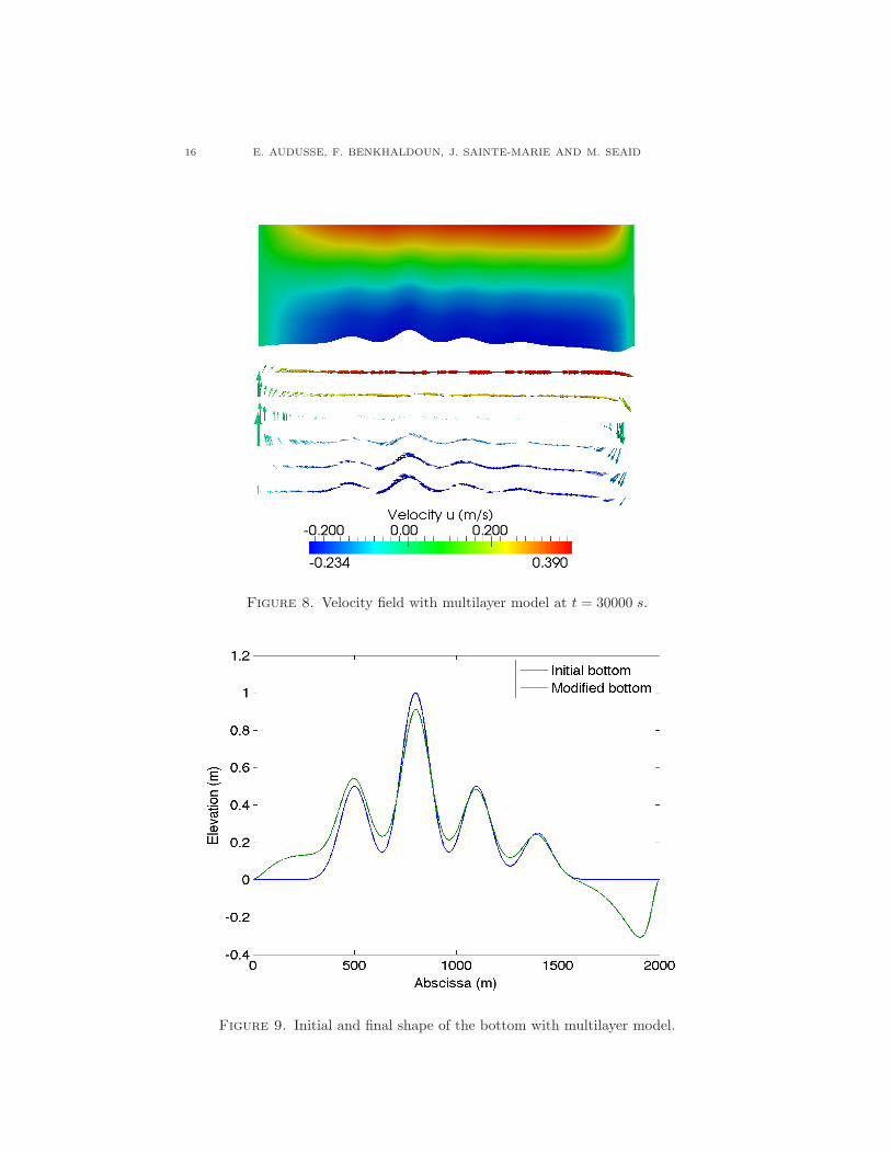
and allows for non zero velocities in the flow. In order to visualize a well establishedwind driven circulation in the basin, we present in Figure 8 the velocity field at timet = 30000 s. Notice that the color in this figure is related to the magnitude of thehorizontal velocity whereas the size of the arrows is related to the norm of thevelocity (even if it does not explicitly appear in the multilayer model, the verticalvelocity is computed in a postprocesing step using for example the divergence freecondition of the incompressible Navier-Stokes equations). A wind driven circulationis clearly detected in the basin. This result is in accordance with what is observed forgeophysical flows in lake or estuaries when the effects due to the density variationin the flow are negligible. Since the hydrodynamic is completely different fromwhat was obtained for the single-layer case, one expects for a very different erosionprocess. In Figure 9 we present the initial and final shape of the bottom of thebasin. It can be observed that a large erosion process takes place near the rightcoast of the basin. We can also observe sediment deposition in the saddles of thetopography and on left coast of the lake. Compared to the single layer approach,the bedload shows a different behavior which in turn affects the dynamic of the flow.This discrepancy on the obtained results is related to the fact that the sedimentdischarge in the Exner equation uses a completely different near-bed velocity field.Notice also that the single-layer approach assumes a uniform velocity along the


Figure 8. Velocity field with multilayer model at t = 30000 s.

Figure 9. Initial and final shape of the bottom with multilayer model.


depth-averaged model which overestimate (during the transient phase) the near-bed velocity resulting in a faster sediment transport compared to the multilayerresults.

5. Concluding Remarks. In this paper we have presented a class of multilayermodels for solving a one-dimensional morphodynamic problem. The model con-sists on coupling the multilyaer Saint-Venant equations for the hydrodynamics withthe Exner equation for the morphodynamics. Forcing terms due to bottom fric-tion, wind shear stresses and exchange between the layers are also included in thecoupled model. For comparison reasons we have also considered the single layersediment transport model. As numerical solvers we have applied a robust finitevolume method for the single layer approach and a kinetic method for the mul-tilayer approach. To verify the considered models we have solved a wind drivenflow in a closed basin. The obtained results exhibit completely different flow andsediment features. The present work may serve as evidence on the limitation of thesingle-layer approach in resolving recirculation flows over movable beds.

Future work will concentrate on validating the proposed model against numericalresults obtained using the three-dimensional incompressible Navier-Stokes equationssubject to kinematic boundary on the bottom and free-surface boundary on thesurface. Furthermore, it is worth emphasizing that, the model problem consideredin the current work is highly idealized, in particular, the bed discharge (16), diffusioneffects and tidal waves as in many coastal scenarios are not accounted for. However,the results make it promising to be applicable also to real situations where, beyondthe many sources of complexity, there is a more severe demand for accuracy inpredicting the morphological evolution, which must be performed for long time.

Acknowledgments. Financial support provided by the project Mhycof, UniversiteParis 13 is gratefully acknowledged.

REFERENCES

[1] Audusse E, Bristeau M.O, A well-balanced positivity preserving second order scheme forshallow water flows on unstructured meshes. JCP. 2005; 206:311–333.

[2] Audusse E, Bouchut F., Bristeau M.O, Klein R., Perthame B., A fast and stable well-balancedscheme with hydrostatic reconstruction for shallow water flows SIAM J. Sci. Comp. 2004;25:2050–2065.

[3] Audusse E, Bristeau M.O, Perthame B., Sainte-Marie J., A multilayer Saint-Venant modelwith mass exchange: Derivation and numerical validation. M2AN . 2010; in press

[4] Benkhaldoun F, Sahmim S, Seaid M, A two-dimensional finite volume morphodynamic modelon unstructured triangular grids. Int. J. Num. Meth. Fluids. 2010; 63:1296–1327. in press.

[5] Bouchut F., Morales de Luna T., An entropy satisfying scheme for two-layer shallow waterequations with uncoupled treatment, M2AN 2008, 42, 683–698.

[6] Benkhaldoun F, Sahmim S, Seaid M, Solution of the Sediment Transport Equations using aFinite Volume Method based on Sign Matrix. SIAM J. Sci. Comp. 2009; 31:2866–2889.

[7] Bermudez A, Rodrıguez C, Vilar M.A, Solving Shallow Water Equations by a Mixed ImplicitFinite Element Method. IMA J Numer Anal. 1991; 11:79–97.

[8] Castro M.J., Macıas J., Pares C., A Q-Scheme for a Class of Coupled Conservation Lawswith Source Term. Application to a Two-layer 1d Shallow Water System, M2AN 2001, 35,107–127.

[9] Crotogino A, Holz K.P. Numerical movable-bed models for practical engineering, AppliedMathematical Modelling 1984; 8:45–49.

[10] J.A. Dutton, The Ceaseless Wind: An Introduction to the Theory of Atmospheric Motion,Dover Publications Inc, 1987.

[11] Grass AJ. Sediment transport by waves and currents. SERC London Cent. Mar. Technol.Report No: FL29 1981


[12] Hudson J, Sweby P.K. Formations for numerically approximating hyperbolic systems govern-ing sediment transport. J. Scientific Computing 2003; 19:225–252.

[13] Meyer-Peter E, Muller R. Formulas for Bed-load Transport, In: Report on 2nd meeting oninternational association on hydraulic structures research, Stockholm. 1948; 8:39–64.

[14] E. Miglio, A. Quarteroni, F. Saleri, Finite Element Approximation of Quasi-3D Shallow WaterEquations, Computer Methods in Applied Mechanics and Engineering, Vol. 174 (1999), 355–369.

[15] Perthame B, Kinetic formulation of conservation laws. Oxford University Press. 2004..[16] Pritchard D, Hogg A.J. On sediment transport under dam-break flow. J. Fluid Mech. 2002;

473:265–274.[17] Rosatti G, Fraccarollo L. A well-balanced approach for flows over mobile-bed with high

sediment-transport. J. Comput. Physics 2006; 220:312–338.[18] Vallis G.K., Atmospheric and oceanic fluid dynamics: fundamentals and large-scale circula-

tion. Cambridge University Press 2006.

Received xxxx 20xx; revised xxxx 20xx.E-mail address: [email protected]

E-mail address: [email protected]



multilayer saint-venant equations over movable beds

Documents