mssm higgs with dimension-six operators
TRANSCRIPT
arX
iv:0
910.
1100
v2 [
hep-
ph]
26
Jan
2010
CPHT-RR106.1009, LPT-Orsay 09-77
CERN-PH-TH/2009-184
MSSM Higgs with dimension-six operators.
I. Antoniadis a,b , E. Dudas b,c , D. M. Ghilencea a, b, †, P. Tziveloglou a, d, 1
aDepartment of Physics, CERN - Theory Division, 1211 Geneva 23, Switzerland.
bCentre de Physique Theorique, Ecole Polytechnique, CNRS, 91128 Palaiseau, France.
cLPT, UMR du CNRS 8627, Bat 210, Universite de Paris-Sud, 91405 Orsay Cedex, France.
d Department of Physics, Cornell University, Ithaca, NY 14853 USA.
Abstract
We investigate an extension of the MSSM Higgs sector by including the effects of all
dimension-five and dimension-six effective operators and their associated supersymmetry
breaking terms. The corrections to the masses of the neutral CP-even and CP-odd Higgs
bosons due to the d= 5 and d= 6 operators are computed. When the d= 5 and d= 6
operators are generated by the same physics (i.e. when suppressed by powers of the
same scale M), due to the relative tanβ enhancement of the latter, which compensates
their extra scale suppression (1/M), the mass corrections from d = 6 operators can be
comparable to those of d = 5 operators, even for conservative values of the scale M .
We identify the effective operators with the largest individual corrections to the lightest
Higgs mass and discuss whether at the microscopic level and in the simplest cases, these
operators are generated by “new physics” with a sign consistent with an increase of mh.
Simple numerical estimates easily allow an increase of mh due to d = 6 operators alone in
the region of 10−30 GeV, while for a much larger increase light new states beyond MSSM
may be needed, in which case the effective description is unreliable. Special attention is
paid to the treatment of the effective operators with higher derivatives. These can be
removed by non-linear field redefinitions or by an “unfolding” technique, which effectively
ensure that any ghost degrees of freedom (of mass >∼M) are integrated out and absent
in the effective theory at scales much smaller than M . Considering general coefficients
of the susy operators with a scale of new physics above the LHC reach, it is possible to
increase the tree-level prediction for the Higgs mass to the LEPII bound, thus alleviating
the MSSM fine-tuning.
† on leave from Theoretical Physics Department, IFIN-HH Bucharest, POBox MG-6, Romania.1 E-mail addresses: [email protected], [email protected],
Contents
1 Introduction 1
2 MSSM Higgs sector with d=5 and d=6 operators 4
3 The scalar potential with d=5 and d=6 operators 8
4 Corrections to the MSSM Higgs masses: analytical results 13
5 Analysis of the leading corrections and effective operators 17
6 Conclusions 21
7 Appendix: 24
A Integrals of operators O1,..8: . . . . . . . . . . . . . . . . . . . . . . . . . . . . . 24
B Integrating out the ghosts, field redefinitions, and “on-shell” operators. . . . . . 26
B.1 The case of d = 6 operators. . . . . . . . . . . . . . . . . . . . . . . . . . 26
B.2 The case of d = 5 operators. . . . . . . . . . . . . . . . . . . . . . . . . . 28
C Coefficients for the Higgs masses. . . . . . . . . . . . . . . . . . . . . . . . . . . 33
D One-loop mh with d = 5 operators . . . . . . . . . . . . . . . . . . . . . . . . . 34
1 Introduction
The coming LHC experiments are a great opportunity to test directly the old idea of low-
energy supersymmetry, as a possibility of new physics beyond the Standard Model. In the
minimal supersymmetric version of this model (MSSM) one obtains definite predictions in
particular for the Higgs sector. For an agreement with the LEPII constraints for the mass
of the SM-like Higgs of mh > 114.4 GeV [1], the MSSM requires that quantum corrections
lift its tree-level bound mh≤mZ . This is indeed possible and acceptable within the allowed
parameter space, increasing the Higgs mass above the LEPII bound (for a recent MSSM fit
see [2]). However, larger quantum corrections usually require larger soft terms, making it
more difficult to satisfy the electroweak constraint v2 = −m2soft/λ with λ the MSSM effective
quartic coupling and m2soft a linear combination of soft (masses)2. With λ fixed by the gauge
sector and with msoft ∼ TeV this condition is more difficult to respect, given the negative
searches for supersymmetry so far and the mass bounds for sparticles. As a result, the MSSM
appears fine-tuned [3, 4, 5, 6] although there is no universally agreed fine-tuning measure or
1
exact value. For further discussion in this direction see [7]. This situation could even be seen
as undermining the original motivation for supersymmetry, prompting alternatives such as [8].
If one maintains the idea of TeV-scale supersymmetry, such a problem of the MSSM must
be addressed. The most common idea to solve it is to assume that new physics beyond the
MSSM is present somewhere in the region of a few TeV. To investigate this possibility, a
general, model-independent approach can be considered, by parametrising this new physics
using effective operators. This is possible by organising such operators in inverse powers of
the scale M of new physics which, when integrated out, generates these effective operators.
One can later address the question of what “new physics” may generate these operators. In
[9] operators of dimension d = 5 were considered in the Higgs sector, together with their
microscopic origin and implications for the Higgs mass (mh). Further analysis including all
baryon and lepton number conserving d = 5 operators beyond MSSM was done in [10, 11],
showing how generalised, spurion dependent field redefinitions reduce the number of effective
operators to an irreducible, minimal set. As a result, the number of independent parameters
is reduced with the benefit of improving the predictive power of the method. Further analysis
of the MSSM with (d = 5) effective operators studied the stability of the Higgs potential
with these operators [12], the effects on the neutralino sector [13], baryogenesis [14], CP
violation [15] or fine-tuning [16]. The presence of these operators of d = 5 can increase the
effective quartic coupling λ of the Higgs field and as a result the fine tuning [18] for the MSSM
electroweak scale is reduced [16] (see also [17]). One obtains one-loop values 114≤mh≤ 130
GeV with a very acceptable fine-tuning ∆≤10 at one-loop, for M∼8 to 10 TeV [16].
The purpose of this work is to extend these studies by considering, in a systematic way,
operators of dimension d = 6 that can account for new physics beyond the MSSM Higgs
sector. The motivation is that such operators can bring relevant contributions to mh, even
in the absence of d = 5 operators. This is indeed possible, since not all d=6 operators are
necessarily generated by the same new physics as the d = 5 ones. Even if both d = 5 and d = 6
operators are present, they could also be suppressed by a different high scale, if generated
by different new physics; this possibility can, in principle, also be read from our results by
keeping track of their coefficients. Finally, if all or some of the d = 5, 6 operators are generated
by same new physics, while suppressed by an extra 1/M factor relative to the leading d=5
operators, the d = 6 operators can nevertheless have an impact for the large tan β region of
the parameter space. Indeed, some d = 6 operators acquire an enhancement factor (tan β)
relative to the d = 5 operators, which compensates for their extra scale suppression. As a
result, their effects on the Higgs mass can be comparable to those of d = 5 operators and
2

it is interesting to examine, in this setup, the new corrections to mh at classical level. The
study is also relevant for examining the limits of the approximation of expanding in powers
of 1/M by comparing leading and sub-leading terms of this expansion. Such corrections to
mh can be as large as loop corrections to mh. We identify individual d = 6 operators with
the largest correction to mh, and discuss their possible microscopic origin and the signs they
are generated with in the simplest cases. Although we do not provide detailed examples of
high-energy physics that give the desired signs, considering general coefficients of the susy
operators of d = 6, our results show that one can increase the tree-level prediction for the
Higgs mass to the LEPII bound (alleviating the fine-tuning of the MSSM as noticed earlier
for d = 5 operators [9, 16]), even for a scale of new physics above the LHC reach.
While studying higher dimensional operators, one problem is associated with the presence
in some of these of higher derivatives, i.e. the presence of ghosts degrees of freedom in the
spectrum. In some cases one can use the equations of motion to set these operators “on-
shell” [19, 20, 21], and remove the extra derivatives. We investigate this procedure and show
that this ultimately means integrating out the ghost degrees of freedom. While this “on-
shell” method is correct in the leading order (in 1/M), it is not true beyond it. Appendix B
provides detailed examples which investigate these issues, and supports this statement (see in
particular Appendix B.2). A more general and correct procedure is to use instead non-linear
field redefinitions to remove the derivative operators. A third and more interesting method
is to re-write (“unfold”) the original theory with higher derivatives as a second-order theory
(i.e. with at most two derivatives) with additional (ghost) superfields of mass of order M
[22]. After integrating classically these fields one obtains in the low energy action below M ,
an effective theory without higher derivatives and with (classically) renormalised interactions.
The results obtained are identical to those obtained by using the non-linear field redefinitions
mentioned earlier; in the leading order in 1/M the method of setting “on-shell” the operators
with extra derivatives by equations of motion gives similar results.
The aforementioned presence of the ghost degrees of freedom near the scale M simply
warns us that beyond this scale the theory is unstable and UV incomplete. This is a generic
situation in all effective theories, even in those obtained from renormalisable ones by inte-
grating out a massive state and after truncating the effective action to a given order (in
1/M). These problems are also present in our discussion with d= 6 operators. In the end,
one eliminates the d=5 operators with extra derivatives via field redefinitions, to leave only
polynomial (in superfields) d=5 operators, and d=6 operators in which it is possible to use
the equations of motion (with a similar result with integrating out the ghost degrees of free-
3
dom). In the presence of supersymmetry breaking additional effects are present, like: µ-term
renormalisation by susy-breaking terms, soft terms renormalisation, discussed in detail in [10].
The plan of the paper is as follows: Section 2 presents the list of operators and clarifies
which of them have relevant contributions to the scalar potential. In Section 3 the scalar po-
tential of the Higgs in MSSM with d=5, 6 operators is computed. Section 4 shows the results
for the masses of the CP even/odd higgses. We identify the operators with the largest contri-
bution in Section 5. The Appendix provides technical details and shows how to replace higher
derivative operators by non-derivative ones in an effective action with d = 5, 6 operators.
2 MSSM Higgs sector with d=5 and d=6 operators
The relevant part of the Lagrangian of our model contains a piece L0 of the MSSM higgs
sector, together with that due to relevant d = 5 and d = 6 operators. For L0 we have
L0 =∫
d4θ∑
i=1,2
Zi(S, S†)H†
i eVi Hi +
{∫
d2θ µ0 (1 +B0 m0 θθ)H1.H2 + h.c.
}
(1)
in a standard notation. Here Zi(S, S†) = 1− cim
20 θθθθ with i = 1, 2 and ci = O(1), m0 is the
supersymmetry breaking scale in the visible sector, m0 = 〈Fhidden〉/MP lanck with Fhidden an
auxiliary field in the hidden sector. As usual we assume this breaking is transmitted to the
visible sector through gravitational interactions mediated by MP lanck.
We extend this Lagrangian by d = 5 and d = 6 operators. In the first class we have
L1 =1
M
∫
d2θ ζ(S) (H2.H1)2+h.c. = 2 ζ10 (h2.h1)(h2.F1 + F2.h1) + ζ11 m0 (h2.h1)
2 + h.c,
L2 =1
M
∫
d4θ{
A(S, S†)Dα[
B(S, S†)H2 e−V1
]
Dα
[
C(S, S†) eV1 H1
]
+ h.c.}
(2)
where1
1
Mζ(S) = ζ10 + ζ11 m0 θθ, ζ10, ζ11 ∼ 1/M, (3)
with S the spurion superfield, S = θθm0. We assume that
m0 ≪M (4)
1Other notations used: in [10] η2=2ζ10µ∗0 , η3=−2m0ζ11; in [16] η2→ζ1, η3→ζ2; in [9] η2→2ǫ1r, η3→2ǫ2r
4
so that the effective theory approach is reliable. If this condition is not respected and the
“new physics” is represented by “light” states (like the MSSM states), then one should work
in the model where these are not integrated out. A,B,C are general functions, which take
into account supersymmetry breaking associated with these operators so, for example:
A(S, S†) = a0 + a1 S + a∗1 S† + a2 S S†, (similar for B,C) (5)
They are general and account for effects of supersymmetry breaking in the presence of some
massive states which when integrated out generate L1,2 with these susy breaking terms.
L2 is eliminated by generalised, spurion-dependent field redefinitions as it was showed
in detail in [10]. We assume this procedure was already implemented, therefore only L1 is
relevant for the discussion below. These redefinitions bring however a renormalisation of the
usual MSSM soft terms and of the µ term, and additional corrections of order 1/M2. The
latter are corrections to the d = 6 operators that are relevant for the Higgs sector, that we
present shortly. Since we shall write down all d = 6 operators, these corrections are then
ultimately accounted for by renormalisations (redefinitions) of the coefficients of the d = 6
terms. Since we take these coefficients arbitrary, without any restriction to generality we can
assume these redefinitions are already implemented.
The list of d = 6 operators is [23]
Oj =1
M2
∫
d4θ Zj(S, S†) (H†
j eVj Hj)
2, j ≡ 1, 2.
O3 =1
M2
∫
d4θ Z3(S, S†) (H†
1 eV1 H1) (H
†2 e
V2 H2),
O4 =1
M2
∫
d4θ Z4(S, S†) (H2.H1) (H2.H1)
†,
O5 =1
M2
∫
d4θ Z5(S, S†) (H†
1 eV1 H1) H2.H1 + h.c.
O6 =1
M2
∫
d4θ Z6(S, S†) (H†
2 eV2 H2) H2.H1 + h.c.
O7 =1
M2
∫
d2θ Z7(S, 0)1
16 g2 κTrWαWα (H2H1) + h.c.
O8 =1
M2
∫
d4θ[
Z8(S, S†) (H2 H1)
2 + h.c.]
(6)
where Wα = (−1/4)D2e−V Dα eV is the chiral field strength of SU(2)L or U(1)Y vector
superfields Vw and VY respectively. Also V1,2 = V aw (σ
a/2)+(∓1/2)VY with the upper (minus)
sign for V1. The expressions of these operators in component form, are given in Appendix A.
5
The remaining d = 6 operators are:
O9 =1
M2
∫
d4θ Z9(S, S†) H†
1 ∇2eV1 ∇2 H1
O10 =1
M2
∫
d4θ Z10(S, S†) H†
2 ∇2eV2 ∇2 H2
O11 =1
M2
∫
d4θ Z11(S, S†) H†
1 eV1 ∇α W (1)
α H1
O12 =1
M2
∫
d4θ Z12(S, S†) H†
2 eV2 ∇α W (2)
α H2
O13 =1
M2
∫
d4θ Z13(S, S†) H†
1 eV1 W (1)
α ∇α H1
O14 =1
M2
∫
d4θ Z14(S, S†) H†
2 eV2 W (2)
α ∇α H2 (7)
Also ∇α Hi = e−Vi Dα eViHi and W i
α is the field strength of Vi. To be even more general,
in the above operators one should actually include spurion dependence under any ∇α, of
arbitrary coefficients to include supersymmetry breaking effects associated to them. Finally,
the wavefunction coefficients introduced above have the structure
1
M2Zi(S, S
†) = αi0 + αi1 m0 θθ + α∗i1 m0 θθ + αi2m
20 θθθθ, αij ∼ 1/M2. (8)
Regarding the origin of these operators: O1,2,3 can be generated in MSSM with an addi-
tional, massive U(1)′ gauge boson or SU(2) triplets integrated out [9]. O4 can be generated
by a massive gauge singlet or SU(2) triplet, while O5,6 can be generated by a combination
of SU(2) doublets and massive gauge singlet. O7 is essentially a threshold correction to the
gauge coupling, with a moduli field replaced by the Higgs. O8 exists only in non-susy case,
but is generated when redefining away the d = 5 derivative operator [10], thus we keep it.
Let us consider for a moment the operators O9,...14 in the exact supersymmetry case. Then,
we can set “on-shell” some of these, by using the eqs of motion2:
−1
4D
2(H†
2 eV2) + µ0H
T1 (iσ2) = 0,
1
4D
2(H†
1 eV1) + µ0H
T2 (iσ2) = 0 (9)
With this we find that in the supersymmetric case 3:
O9 ∼∫
d4θ H†1∇
2eV1 ∇2H1 = 16 |µ0|2
∫
d4θH†1 e
V1 H1. (10)
2 Superpotential convention:∫d2θµ0 H1.H2 =
∫d2θ µ0 H
T1 (iσ2)H2 ≡
∫d2θ µ0 ǫ
ij Hi1 H
j2; ǫ12 = 1 = −ǫ21.
3Also using (iσ2) e−Λ = eΛ
T
(iσ2); Λ ≡ Λa T a; (iσ2)T = −(iσ2); (iσ2)
2 = −12
6
and similar for O10. Regarding O11,12, in the supersymmetric case they vanish, following the
definition of ∇α and an integration by parts. Further, O13,14 are similar to O9,10, which can
be seen by using the definition of W(i)α and the relation between ∇2, (∇2
) and D2, (D2).
In conclusion, in the exact supersymmetric case, O9...14 give at most wavefunction renor-
malisations of operators already included. This was shown by using the equations of motion
(“on-shell” method – we return to this issue shortly). Let us now consider supersymmetry
breaking associated to these operators, due to their spurion dependence. Turning on super-
symmetry breaking should not bring physical effects, as showed explicitly in [10] and could
only give soft terms and µ-term renormalisation by O(1/M2) corrections. Since these terms
are anyway renormalised by O1,...8, where spurion dependence is included with arbitrary co-
efficients, then there is no loss of generality to ignore the supersymmetry breaking effects
associated to O9,...14 in the following discussion, which are anyway taken into account by
O1,..8. Following this discussion, one concludes that O9,...,14 are not relevant for the anal-
ysis of the Higgs potential performed below. Finally, there can be an additional operator
of d = 6 from the gauge sector, O15 = (1/M2)∫
d2θ Wα2Wα which could affect the Higgs
potential4. Using the equations of motion for the gauge field it can be shown that O15 gives
a renormalisation of O1,2,3, so its effects are ultimately included, since the coefficients Z1,2,3
are arbitrary.
The careful reader may question the above use of the eqs of motion in some of the higher
dimensional operators, in order to essentially remove those with more than two derivatives
(O9,..,15). This “on-shell”procedure is justified by previous works [19, 20] and further detailed
in [21]. A more general and correct approach is to use instead non-linear field redefinitions5
or an “unfolding” technique (see later). These two generally valid approaches are discussed
in detail in Appendix B. We used these two approaches to check the validity of the above
“on-shell” procedure, for the cases and approximation in which we applied it. This was also
done to clarify, from a general perspective, what actually means to set “on-shell” the higher
derivative operators.
To this purpose, consider for simplicity the case of operator O9 without gauge fields,
when O9 ∼ (1/M2)∫
d4θ H†12H1. A Lagrangian with such a higher derivative operator
contains additional poles corresponding to ghosts degrees of freedom. As shown in [22], see
also Appendix B.1, such theory can be reformulated and “unfolded” into a second order one
(i.e with no more than two derivatives) with (one or two) additional ghost superfields of mass
4Its complete gauge invariant form is∫d4θ T r eV Wαe−V D2(eV Wαe
−V ).5These are actually employed to prove this “on-shell” method [21].
7
of the order M . In such an effective theory, at energies well below the scale M , such ghost-like
states can then be integrated out. The result is a wavefunction renormalisation only, which is
in agreement with the result obtained by the “on-shell” method discussed above. Therefore,
using the eqs of motion to set “on-shell” the higher derivative operator as done in (9), (10)
corresponds to integrating out the massive ghost degrees of freedom associated with such
operator. For details see Appendix B.1.
A result similar to the “unfolding” method is obtained by using non-linear field redefini-
tions. This was detailed in Appendix B.2 for the case of d = 5 operators. There it is shown
that in the leading order in 1/M the “unfolding” method (integrating out the ghosts), the
nonlinear field redefinition method and the “on-shell” method give similar results. Beyond
this 1/M order however, the “on-shell” method should be appropriately modified to use the
Euler-Lagrange equations for a higher derivative Lagrangian.
With these clarifications one can safely say that O9,...,15 are not relevant for the following
discussion of the Higgs potential. In conclusion the list of d = 6 operators that remain for
our study of the Higgs sector beyond MSSM is that of eq.(6). Let us stress that not all the
remaining operators O1,..,8 of (6) are necessarily present or generated in a detailed model.
Symmetries and details of the “new physics” beyond the MSSM that generated them, may
forbid or favour the presence of some of them. Therefore, we regard these remaining operators
as independent of each other, although in specific models correlations may exist among their
coefficients Zi. It is important to keep all these operators in the analysis, for the purpose of
identifying which of them has the largest individual contribution to the Higgs mass, which is
one of the main interests of this analysis. Finally, some of the d = 6 operators can in principle
be present even in the absence of the d = 5 operators, if these classes of operators are generated
by integrating different “new physics”. In specific models one simply sets to zero, in the results
below, the coefficients of those operators of d=5 and/or d=6 not present/generated.
3 The scalar potential with d=5 and d=6 operators
Following the previous discussion, the overall Lagrangian of the model is
LH = L0 + L1 +8∑
i=1
Oi (11)
with the MSSM higgs Lagrangian L0 of eq.(1), L1 of eq.(2) and O1,2,....,8 of eq.(6).
8
With the results in Appendix A we find the following contributions to the scalar potential:
VF =∂2 K
∂ hi ∂ h∗jFi F
∗j = |F1|2 + |F2|2 +
∂2 K6
∂ hi ∂ h∗jFi F
∗j (12)
where K6 is the contribution of O(1/M2) to the Kahler potential due to O1,...8. The first two
terms in the rhs give (hi denote SU(2)L doublets, |hi|2 ≡ h†i hi):
VF,1 ≡ |F1|2 + |F2|2
= |µ0 + 2 ζ10 h1.h2|2(
|h1|2 + |h2|2)
+[
µ∗0
(
|h1|2 ρ21 + |h2|2 ρ11 + (h1.h2)† (ρ22 + ρ12)
)
+ h.c.]
(13)
obtained using (A-11) and where ρij are functions of h1,2:
ρ11 = −(2α10 µ0 + α40µ0 + α∗51 m0)|h1|2 − (α30 µ0 + α40µ0 + α∗
61 m0) |h2|2
−(α∗41 m0 + α∗
50 µ0) (h2.h1)∗ +
[
(α60 + 2α50)µ0 + 2α∗81 m0
]
(h1.h2)
ρ12 = (2α∗11 m0 + α∗
50 µ0)|h1|2 + (α∗31 m0 + α∗
50 µ0) |h2|2
−[
(2α10 + α30)µ0 + α∗51 m0
]
(h1.h2) + α∗51 m0 (h2.h1)
∗ (14)
ρ21 = −(2α20 µ0 + α40µ0 + α∗61 m0)|h2|2 − (α30 µ0 + α40µ0 + α∗
51 m0) |h1|2
−(α∗41 m0 + α∗
60 µ0) (h2.h1)∗ +
[
(α50 + 2α60)µ0 + 2α∗81 m0
]
(h1.h2)
ρ22 = (2α∗21 m0 + α∗
60 µ0)|h2|2 + (α∗31 m0 + α∗
60 µ0) |h1|2
−[
(2α20 + α30)µ0 + α∗61 m0
]
(h1.h2) + α∗61 m0 (h2.h1)
∗ (15)
The non-trivial field-dependent Kahler metric gives for the last term in VF of eq.(12):
VF,2 = |µ0|2[
2(
α10 + α20 + α40
)
|h1|2 |h2|2 + (α30 + α40)(
|h1|4 + |h2|4)
+2(
α10 + α20 + α30
)
|h1.h2|2 +(
|h1|2 + 2 |h2|2)(
α50 h2.h1 + h.c.)
+(
2|h1|2 + |h2|2)(
α60 h2.h1 + h.c.)
]
(16)
so that VF = VF,1 + VF,2. Further, for the gauge contribution, we have:
9
Vgauge =1
2
(
D2w +D2
Y )[
1 + (α70 h2.h1 + h.c.)]
=g21 + g22
8
(
|h1|2 − |h2|2) [(
1 + f1(h1,2)) |h1|2 − (1 + f2(h1,2)) |h2|2]
+g222
(1 + f3(h1,2))|h†1 h2|2 (17)
obtained with (A-12) and where f1,2,3 are functions of h1,2:
f1(h1,2) ≡ 4α10 |h1|2 +[
(2α50 − α70)h2.h1 + h.c.)]
f2(h1,2) ≡ 4α20 |h2|2 +[
(2α60 − α70)h2.h1 + h.c.)]
f3(h1,2) ≡ ρ1 + ρ2 + (α70 h2.h1 + h.c.) (18)
with
ρ1(h1,2) ≡ 2α10 |h1|2 + α30 |h2|2 +[
(α50 − α70) h2.h1 + h.c.]
ρ2(h1,2) ≡ 2α20 |h2|2 + α30 |h1|2 +[
(α60 − α70) h2.h1 + h.c.]
(19)
The scalar potential also has corrections VSSB from supersymmetry breaking, due to
spurion dependence in higher dimensional operators (of dimensions d = 5 and d = 6); in
addition we also have the usual soft breaking term from the MSSM. As a result
VSSB = −m20
[
α12 |h1|4 + α22 |h2|4 + α32 |h1|2 |h2|2 + α42 |h2.h1|2 (20)
+(
α52 |h1|2 (h2.h1) + h.c.)
+(
α62 |h2|2 (h2.h1) + h.c.)
]
−[
m20 α82 (h1.h2)
2 + ζ11 m0 (h2.h1)2 + µ0 B0m0 (h1.h2)+h.c.
]
+m20 (c1|h1|2 +c2|h2|2)
Finally, in O1,...8 there are non-standard kinetic terms that can contribute to V when the
scalar singlet components (denoted h0i ) of hi acquire a vev. The relevant terms are:
LH ⊃ (δij∗ + gij∗) ∂µ h0i ∂
µh0∗j , i, j = 1, 2. (21)
where the field dependent metric is:
g11∗ = 4α10 |h01|2 + (α30 + α40) |h02|2 − 2 (α50 h01 h
02 + h.c.)
g12∗ = (α30 + α40)h0∗1 h02 − α∗
50 h0∗21 − α60 h0 22 , g21∗ = g∗12∗
g22∗ = 4α20 |h02|2 + (α30 + α40) |h01|2 − 2 (α60 h01 h
02 + h.c.) (22)
10
For simplicity we only included the SU(2) higgs singlets contribution, that we actually need
in the following, but the discussion can be extended to the general case. The metric gij∗ is
expanded about a background value 〈h0i 〉 = vi/√2, then field re-definitions are performed to
obtain canonical kinetic terms; these bring further corrections to the scalar potential. The
field re-definitions are:
h01 → h01
(
1− g11∗
2
)
− g21∗
2h02
h02 → h02
(
1− g22∗
2
)
− g12∗
2h01, gij∗ ≡ gij∗
∣
∣
∣
h0i→vi/
√2
(23)
Since the metric has corrections which are O(1/M2), after (23) only the MSSM soft breaking
terms and the MSSM quartic terms are affected. The other terms in the scalar potential,
already suppressed by one or more powers of the scale M are affected only beyond the ap-
proximation O(1/M2) considered here. Following (23) the correction terms O(1/M2) induced
by the MSSM quartic terms and by soft breaking terms in VSSB are:
Vk.t. = m21 (−g∗11) |h01 |2 + m2
2 (−g∗22) |h02 |2 −1
2
(
m21 + m2
2
) (
g21∗ h0∗1 h02 + h.c.
)
+1
2
[
B0 m0 µ0
(
(g11∗ + g22∗) h01 h
02 + g12∗ h
0 21 + g21∗ h
0 22
)
+ h.c.]
− g2
8
(
|h01 |2 − |h02 |2) (
g11∗ |h01 |2 − g22∗ |h02 |2 + h.c.)
(24)
Using eqs.(11), (12), (13), (16), (17), (21), (24), we find the full scalar potential. With the
notation m2i ≡ cim
20 + |µ0|2, i = 1, 2 (c1,2, were introduced in Zi of eq.(1)) one has:
V = VF,1 + VF,2 + VG + VSSB + Vk.t. (25)
= Vk.t. + m21|h1|2 + m2
2|h2|2 −[
µ0 B0m0 h1 · h2 + h.c.]
+λ1
2|h1 |4 +
λ2
2|h2 |4 + λ3 |h1 |2 |h2 |2 + λ4 |h1 · h2 |2
+( λ5
2(h1 · h2)2 + λ6 |h1 |2 (h1 · h2) + λ7 |h2 |2 (h1 · h2) + h.c.
)
+g2
8
(
|h1|2 − |h2|2)(
f1(h1,2) |h1|2 − f2(h1,2) |h2|2)
+ 4 |ζ10|2|h1.h2|2 (|h1|2 + |h2|2)
+g222
f3(h1,2) |h†1h2|2
where g2 = g21 + g22 , and f1,2,3(h1,2) are all quadratic in hi, see eq.(18). Except Vk.t., all other
fields are in the SU(2) doublets notation. The following notation for λi was introduced:
11
λ1/2 = λ01/2− |µ0|2 (α30 + α40)−m2
0 α12 − 2m0 Re[
α51 µ0
]
(26)
λ2/2 = λ02/2− |µ0|2 (α30 + α40)−m2
0 α22 − 2m0 Re[
α61 µ0
]
λ3 = λ03 − 2 |µ0|2 (α10 + α20 + α40)−m2
0 α32 − 2m0 Re[
(α51 + α61)µ0
]
λ4 = λ04 − 2 |µ0|2 (α10 + α20 + α30)−m2
0 α42 − 2m0 Re[
(α51 + α61)µ0
]
λ5/2 = −m0 µ0 (α51 + α61)−m0 ζ11 −m20 α82
λ6 = |µ0|2 (α50 + 2α60) +m20 α52 +m0 µ0 (2α11 + α31 + α41) + 2m0 µ
∗0 α
∗81 + 2 ζ10 µ
∗0
λ7 = |µ0|2 (α60 + 2α50) +m20 α62 +m0 µ0 (2α21 + α31 + α41) + 2m0 µ
∗0 α
∗81 + 2 ζ10 µ
∗0
Eq.(26) shows the effects of various higher dimensional operators on the scalar potential. As
a reminder, note that all αik ∼ O(1/M2), while ζ11, ζ10 ∼ O(1/M). The latter can dominate,
but this depends on the value of tan β; when this is large, O(1/M2) have comparable size. In
specific models correlations exist among these coefficients. The above remarks apply to the
case when the d = 5 and d = 6 operators considered are generated by the same “new physics”
beyond the MSSM (i.e. are suppressed by the same scale). However, as mentioned earlier,
this may not always be the case; in various models contributions from some d = 6 operators
can be independent of those from d = 5 operators (and present even in the absence of the
latter), if generated by different “new physics”. A case by case analysis is then needed for a
thorough analysis of all possible scenarios for “new physics” beyond the MSSM higgs sector.
We also used the following notation for the corresponding MSSM contribution:
λ01/2 =
1
8(g22 + g21), λ0
2/2 =1
8(g22 + g21), λ0
3 =1
4(g22 − g21), λ0
4 = −1
2g22 , (27)
One can include MSSM loop corrections by replacing λ0i with radiatively corrected values [24].
The overall sign of the h6 terms depends on the relative size of αj0, j = 1, 2, 5, 6, 7, and
cannot be fixed even locally, in the absence of the exact values of these coefficients of the d = 6
operators. Effective operators of d = 5, (ζ10), also contribute to the overall sign, however these
alone cannot fix it. At large fields values higher and higher dimensional operators become
relevant and contribute to it. We therefore do not impose that V be bounded from below at
large fields. For a discussion of stability with d = 5 operators only see [12].
Eqs.(25), (26) of V in the presence of d = 5, 6 effective operators are the main result of this
section. For simplicity, one can take g12∗ , g21∗ real (similar for B0µ0), possible if for example
α50, α60 are real and no vev for Imhi; in the next section we shall assume that this is the case.
12
4 Corrections to the MSSM Higgs masses: analytical results
With the general expression for the scalar potential we compute the mass spectrum. From
the scalar potential, one evaluates the mass of CP-even Higgs fields h,H:
m2h,H ≡
1
2
∂2V
∂h0i ∂h0j
∣
∣
∣
∣
〈hi〉=vi/√2,〈 Im hi〉=0
(28)
In the leading order O(1/M) one has (upper signs for mh):
m2h,H =
m2Z
2+
B0m0µ0(u2 + 1)
2u∓√w
2+ v2
[
(2 ζ10 µ0) q±1 + (−2m0 ζ11) q
±2
]
+ δm2h,H (29)
with
q±1 =1
4u2 (1 + u2)√w
×[
− (1− 6u2 + u4)u√w ∓
(
m2Zu(1− 14u2 + u4)−B0 m0µ0(1 + u2)(1 + 10u2 + u4)
)]
q±2 = ∓ 2u
(1 + u2)2√w
[
−B0m0µ0(1 + u2)−m2Z u]
(30)
where
w ≡ m4Z +
[
−B0m0 µ0(1 + u2)3 + 2m2Zu(1− 6u2 + u4)
](−B0m0µ0)
u2(1 + u2), u ≡ tan β (31)
In eq.(29)
δm2h,H = O(1/M2) (32)
and we also used that mZ = g v/2. One also shows that the Goldstone mode has mG = 0 and
the pseudoscalar A has a mass:
m2A =
1 + u2
uB0 m0 µ0 −
1 + u2
uζ10 µ0 v
2 + 2m0 ζ11 v2 + δm2
A, δm2A = O(1/M2) (33)
The corrections O(1/M) of mh,H and mA showed in (29), (33), agree with earlier findings [9].
Ignoring for the moment the corrections O(1/M2), one eliminates B0 between (29) and
(33) to obtain:
13
m2h,H =
1
2
[
m2A +m2
Z ∓√w]
+ (2 ζ10 µ0) v2 sin 2β
[
1± m2A +m2
Z√w
]
+(−2 ζ11 m0) v
2
2
[
1∓ (m2A −m2
Z) cos2 2β√
w
]
+ δ′m2h,H , δ′m2
h,H = O(1/M2) (34)
where the upper (lower) signs correspond to h (H) respectively and
w ≡ (m2A +m2
Z)2 − 4m2
Am2Z cos2 2β (35)
in agreement with [9]. This is important if one considers mA as an input; it is also needed if
one considers the limit of large tan β at fixed mA (see later).
Regarding the O(1/M2) corrections of δm2h,H , δm2
A and δ′m2h,H of eqs.(29), (33), (34)
in the general case of including all operators and their associated supersymmetry breaking,
they have a rather complicated form. For most purposes, an expansion in 1/ tan β of δm2h,H ,
δm2A, δ
′m2h,H is accurate enough. The reason for this is that it is only at large tan β that
d = 6 operators bring corrections comparable to those of d = 5 operators. The relative tan β
enhancement of O(1/M2) operators compensates for the extra suppression factor 1/M that
these operators have relative to O(1/M) operators (which involve both h1 and h2 and thus
are not enhanced in this limit). Note however that in some models only d = 6 operators may
be present, depending on the details of the “new physics” generating the effective operators.
If we neglect the susy breaking effects of d = 6 operators (i.e. αj1 = αj2 = 0, αj0 6= 0,
j = 1, ..., 8) and with d = 5 operators contribution, one has6 for the correction δm2h,H in
eq.(29) (upper signs correspond to δm2h)
δm2h,H =
7∑
j=1
γ±j αj 0 + γ±x ζ10 ζ11 + γ±z ζ210 + γ±y ζ211 (36)
The expressions of the coefficients γ± are provided in Appendix C and can be used for numeri-
cal studies. While these expressions are exact, they are complicated and not very transparent.
It is then instructive to analyse an approximation of the O(1/M2) correction as an expansion
in 1/ tan β. We present in this limit the correction δm2h,H of eq.(29), which also includes all
supersymmetry breaking effects associated with all d = 5, 6 operators, (i.e. αj1 6= 0, αj2 6= 0,
ζ11 6= 0, j = 1, ..8) in addition to the MSSM soft terms. This has a simple expression:
6In the case of including the supersymmetry breaking effects from effective operators, associated with
coefficients αj1, αj2 j = 1, 2, ..8, the exact formula is very long and is not included here.
14

δm2h = −2 v2
[
α22m20 + 2α61 m0µ0 + (α30 + α40)µ
20 − α20 m
2Z
]
+v2
tan β
[
4α62 m20 + 4µ0 m0 (2α21 + α31 + α41 + 2α81) + 4µ2
0 (2α50 + α60)
− m2Z (2α60 − 3α70)−
v2
(B0m0µ0)(2ζ10 µ0)
2]
+O(1/ tan2 β) (37)
which is obtained with (B0m0µ0) kept fixed. The result is dominated by the first line, including
both susy and non-susy terms from the effective operators. This correction can be comparable
to linear terms in ζ10, ζ11 from d = 5 operators for (2 ζ10µ0) ≈ 1/ tan β (see later). Not all
O1,2...8 are necessarily present, so in some models some αij , ζ10, ζ11 could vanish. Also:
δm2H = −1
4(B0m0µ0) v
2 α60 tan2 β +v2 tan β
8
[
− 8B0m0µ0 α20 − 4α62m20
− 4µ0 m0(2α21 + α31 + α41 + 2α81)− 4µ20 (2α50 + α60) + (2α60 − α70)m
2Z
]
+3
4B0m0µ0 v
2(α50 + α60) +v2
8 tan β
[
− 8B0m0µ0α10 + (12α52 − 16α62)m20
− 4µ0m0(−6α11 + 8α21 + α31 + α41 + 2α81)− 4µ20(5α50 − 2α60)
+ (6α50 + 20α60 − 13α70)m2Z +
8 v2
B0m0µ0(2 ζ10 µ0)
2]
+O(1/ tan2 β) (38)
which is obtained for (B0m0µ0) fixed. Note the O(1/M2) effects from d = 5 operators (ζ210).
Similar expressions exist for the neutral pseudoscalar A. The results are simpler in this
case and we present the exact expression of δm2A of (33) in the most general case, that includes
all supersymmetry breaking effects from the operators of d = 5, 6 and from the MSSM. One
finds
δm2A =
v2
8 tan2 β (1 + tan2 β)
[
− 2B0 m0µ0 α50 +[
− (4α31 + 4α41 + 8α81 + 8α11)m0µ0
− 4α52m20 − 8B0m0µ0α10 − 4 (α50 + 2α60)µ
20 + (2α50 − α70)m
2Z
]
tan β
+[
2B0 m0 µ0 (10α50 + 3α60) + 16α82m20 + 16(α51 + α61)m0 µ0
]
tan2 β
+ 2[
− 4B0 m0µ0(α10 + α20 + 2α30 + 2α40)− 6(α50 + α60)µ20 − (α50 + α60 − α70)m
2Z
− 2(α62 + α52)m20 − 4(α11 + α21 + α31 + α41 + 2α81)m0µ0
]
tan3 β
+[
2B0 m0 µ0 (3α50 + 10α60) + 16α82m20 + 16(α51 + α61)m0µ0
]
tan4 β
−[
8B0 m0µ0 α20 + 4 (2α50 + α60)µ20 − (2α60 − α70)m
2Z + 4α62 m
20
+ 4 (2α21 + α31 + α41 + 2α81)m0 µ0
]
tan5 β − 2B0 m0 µ0 α60 tan6 β]
(39)
15
We also showed that δmG = 0 so the Goldstone mode remains massless in O(1/M2), which
is a good consistency check. A result similar to that in eq.(37) is found from an expansion of
(39) in the large tan β limit:
δm2A = −1
4(B0m0µ0)α60 v
2 tan2 β +tan β
8v2[
− 8B0m0µ0α20 − 4α62m20
− (8α21 + 4α31 + 4α41 + 8α81)m0µ0 − (8α50 + 4α60)µ20 + 2α60 m
2Z − α70 m
2Z
]
+v2
4
[
B0m0µ0(3α50 + 11α60) + 8m20α82 + 8m0µ0(α51 + α61)
]
+v2
8 tan β
[
− 8B0m0µ0 (α10 + 2α30 + 2α40)− 4 (2α11 + α31 + α41 + 2α81) m0µ0
− 4α52 m20 − (4α50 + 8α60)µ
20 − (2α50 + 4α60 − 3α70)m
2Z
]
+O(1/ tan2 β) (40)
We emphasise that the large tan β limits presented so far were done with (B0 m0µ0) fixed.
While this is certainly an interesting case, because then mA becomes large7 a more physical
case to consider at large tan β is that in which one keeps mA fixed (B0m0µ0 arbitrary).
We present below the correction O(1/M2) to m2h,H for the case mA is kept fixed to an ap-
propriate value. The result is (assuming mA>mZ , otherwise δ′m2
h and δ′m2H are exchanged):
δ′m2h = −2 v2
[
α22 m20 + (α30 + α40)µ
20 + 2α61 m0 µ0 − α20 m
2Z
]
− (2 ζ10 µ0)2 v4
m2A −m2
Z
+v2
tan β
[
1
(m2A −m2
Z)
(
4m2A
(
(2α21+α31+α41+2α81)m0 µ0+(2α50+α60)µ20 + α62 m
20
)
− (2α60 − 3α70)m2Am2
Z − (2α60 + α70)m4Z
)
+8 (m2
A +m2Z) (µ0m0 ζ10 ζ11) v
2
(m2A −m2
Z)2
]
+ O(1/ tan2 β) (41)
A similar formula exists for the correction to mH :
δ′m2H =
[
− 2(
m0µ0 (α51 + α61) + α82 m20
)
v2 +(2 ζ10 µ0)
2 v4
m2A −m2
Z
]
+v2
tan β
[ 1
m2A−m2
Z
(
2m2A
(
2 (α11−α21)m0µ0 +(α60−α50)µ20 +(α52−α62)m
20 − α60 m
2A
)
−[
4 (α11 + α21 + α31 + α41 + 2α81)m0µ0 + 6(α50 + α60)µ20 + 2(α52 + α62)m
20
− (α50+5α60−2α70)m2A
]
m2Z − (α50− α60)m
4Z
)
− 8 (m2A +m2
Z) (µ0 m0 ζ10 ζ11) v2
(m2A −m2
Z)2
]
+ O(1/ tan2 β) (42)
7and thus likely to re-introduce a little hierarchy to explain.
16
Corrections (41), (42) must be added to the rhs of eq.(34) to obtain the value of m2h,H
expressed in function of mA fixed. The corrections in eqs.(36) to (42) extend the result in [9]
to include all O(1/M2) terms and represent the main result of this section.
From eqs.(37), (41) we are able to identify the effective operators of d = 6 that give the
leading contributions to m2h, which is important for model building. These are O2,3,4 in the
absence of supersymmetry breaking andO2,6 when this is broken, see also eqs.(6). It is however
preferable to increase m2h by supersymmetric rather than supersymmetry-breaking effects of
the effective operators, because the latter are less under control in the effective approach
and one would favour a supersymmetric solution to the fine-tuning problem associated with
increasing the MSSM Higgs mass above the LEPII bound. Therefore O2,3,4 are the leading
operators, with the remark that O2 has a smaller effect, of order (mZ/µ0)2 relative to O3,4
(for similar αj0, j = 2, 3, 4). At smaller tan β, O5,6 can also give significant contributions,
while O7 has a relative suppression factor (mZ/µ0)2.
5 Analysis of the leading corrections and effective operators
In general one would expect that d = 6 operators give sub-leading contributions to the spec-
trum, compared to d = 5 operators, in the case that all these operators are present and
originate from integrating the same massive “new physics” (i.e. are suppressed by powers of
the same scale M , which is not always the case). Even so, for large tan β the latter acquire a
relative suppression factor, and the two classes of operators can indeed give comparable correc-
tions. At large tan β with mA fixed, by comparing O(1/M) terms in eq.(34) against O(1/M2)
terms in eqs.(41), (42), one identifies the situation when these two classes of operators give
comparable corrections:
4m2A
m2A −m2
Z
| ζ10 µ0 |tan β
≈∣
∣
∣
∣
α22m20 + (α30 + α40)µ
20 + 2α61m0µ0 − α20m
2Z +
2 (ζ10 µ0)2 v2
m2A −m2
Z
∣
∣
∣
∣
∣
∣
∣
∣
ζ11m0 +4m2
Z
m2A −m2
Z
ζ10 µ0
tan β
∣
∣
∣
∣
≈∣
∣
∣
∣
(
m0µ0 (α51 + α61) + α82 m20
)
− 2 (ζ10 µ0)2 v2
m2A −m2
Z
∣
∣
∣
∣
(43)
In this case O(1/(M tan β)) and O(1/M2) corrections are approximately equal (for M ≈m0 tan β). Similar relations can be obtained from comparing (29), (33), against δm2
h,H of (37),
(38), (39). Note that if these relations are satisfied this does not necessarily mean a failure
of the effective field theory expansion, since the “new physics” that generates these operators
17
may be different! Indeed, the corrections from d = 6 and d = 5 operators can be completely
independent (uncorrelated). However, if all operators involved in (43) are generated by the
same massive physics, one would expect that the lhs be smaller than the rhs. In this case one
obtains conditions for the coefficients of the operators that should be considered in numerical
analyses. The exact form of such conditions depends on which operators are present8. Note
that operators with d > 6 could not acquire a tan β enhancement relative to d = 6 operators
to become comparable in size, and they will always have an extra suppression factor (∼ 1/M).
Let us now examine more closely the corrections to the Higgs masses due to d = 6 oper-
ators. The interest is to maximise the correction to the MSSM classical value of mh. From
eq.(37) and (41) and their αij dependence and ignoring susy breaking corrections (αjk, k 6= 0),
we saw that O3,4 bring the largest correction (at large tan β), and to a lower extent also O2.
At smaller tan β, O5,6,7 can have significant corrections. All this can be seen from the relative
variation:
ǫrel ≡mh −mZ
mZ=√
δrel − 1, where
δrel ≡ 1− 4m2A
m2A −m2
Z
1
tan2 β+
v2
m2Z
{
2 ζ10 µ0
tan β
4m2A
m2A −m2
Z
+(−2 ζ11 m0)
tan2 β
2 (m4A +m4
Z)
(m2A −m2
Z)2
−[
2(
α22 m20 + (α30 + α40)µ
20 + 2α61 m0 µ0 − α20 m
2Z
)
+(2 ζ10 µ0)
2 v2
m2A −m2
Z
]
+1
tan β
1
m2A −m2
Z
[
4m2A µ0
(
(2α21 + α31 + α41 + 2α81)m0 + (2α50 + α60)µ0
)
+ 4α62 m20m
2A −(2α60−3α70)m
2Am2
Z − (2α60+α70)m4Z+8 ζ10 ζ11 µ0 m0 v
2m2A+m2
Z
m2A−m2
Z
]
}
+ O(1/ tan4 β) +O(m/(M tan3 β)) +O(m2/(M2 tan2 β)) (44)
where m is some generic mass scale of the theory such as µ0, mZ , m0, v. The arguments of
the functions O in the last line show explicitly the origin of these corrections (MSSM, d = 5
or d = 6 operators, respectively). Depending on the signs of coefficients αjk, ζ10, ζ11 this
relative variation can be positive and increase mh above the MSSM classical upper bound
(mZ). Eq.(44) gives the overall relative change of the classical value of mh in the presence
of all possible higher dimensional operators of d = 5 and d = 6 beyond the MSSM Higgs
8As an example, assuming at least one d = 6 operator is generated by the same physics as the d = 5 one
considered, and if we neglect the supersymmetry breaking associated effects, then from (43) d = 6 operators
could give comparable corrections for |2 ζ10 µ0 | ≈ g2/ tan β ≈ 0.55/ tan β orM ≈ 2µ0 tanβ/g2 ≈ 3.6×µ0 tanβ.
18
sector, for large tan β with mA fixed. The expansion is accurate enough to be used also at
intermediate tan β, but this also depends on the ratio m/M ; for small tan β the terms in the
last line in (44) give an error estimate; alternatively one can use exact δm2h,H in (36).
A similar result exists for the case the limit of large tan β is taken with (B0m0µ0) fixed
(instead of mA). Then
δrel ≡ 1− 4
tan2 β+
v2
m2Z
{
4 (2 ζ10 µ0)
tan β+
2
tan2 β
(
(−2 ζ11 m0) +2m2
Z (2 ζ10 µ0)
B0 m0 µ0
)
− 2[
α22 m20 + 2α61 m0 µ0 + (α30 + α40)µ
20 − α20 m
2Z
]
+1
tan β
[(2 ζ10 µ0)2 v2
−B0 m0 µ0
+ 4 (2α21+α31+α41+2α81)m0 µ0 + 4 (2α50+α60)µ20+4α62 m
20 − (2α60−3α70)m
2Z
]
}
+ O(1/ tan4 β) +O(m/(M tan3 β)) +O(m2/(M2 tan2 β)) (45)
which can be used in numerical applications even for smaller, intermediate values of tan β.
In (44), (45), the d = 6 operators (αij dependence) give contributions which are dominated
by tan β-independent terms. One particular limit to consider for δm2h or δ′m2
h is that in which
the effective operators of d = 6 have coefficients such that these contributions or those in the
first line in (37), (41) add up to maximise δrel. Since coefficients αij are not known, as an
example we can choose them equal in absolute value
− α22 = −α61 = −α30 = −α40 = α20 > 0 (46)
In this case, at large tan β:
δm2h ≈ 2 v2α20
[
m20 + 2m0µ0 + 2µ2
0 + m2Z
]
(47)
and similar for δ′m2h. A simple numerical example is illustrative. For m0 = 1 TeV, µ0 = 350
GeV, and with v ≈ 246 GeV, one has δm2h ≈ 2.36α20 × 1011 (GeV)2. Assuming M = 10 TeV
and ignoring d = 5 operators, with α20 ∼ 1/M2 and the MSSM value of mh taken to be its
upper classical limit mZ (reached for large tan β), we obtain an increase of mh from d = 6
operators alone of about ∆mh = 12.15 GeV to mh ≈ 103 GeV. An increase of α20 by a factor
of 2.5 to α20 ∼ 2.5/M2 would give ∆mh ≈ 28 GeV to mh ≈ 119.2 GeV, which is above the
LEPII bound. Note that this increase is realised even for a scale M of “new physics” beyond
the LHC reach.
Considering instead the larger, loop-corrected MSSM value of mh, to which we add the
d = 6 operators effects, the relative increase of ∆mh due to d = 6 operators alone is mildly
19
reduced. However, the effective operators of d = 6 could in this case reduce the amount of
fine-tuning for the electroweak scale, since these operators can increase the effective quartic
coupling of the Higgs and thus reduce the fine-tuning, even for a smaller increase of mh.
This was indeed observed for the case of d = 5 operators in the presence of MSSM quantum
corrections to mh, when the overall mass of mh (see Appendix D) can easily reach values of
130 GeV with a reduced, acceptable fine-tuning (less than 10 [18]) of the electroweak scale
[16] (for a scale of effective operators close to 10 TeV). A similar result may be expected in
the presence of d = 6 operators [25]. Finally, the above choice of M = 10 TeV was partly
motivated by the fine-tuning results of [16] (valid for d = 5 operators) and also on convergence
grounds: the expansion parameter of our effective analysis is mq/M where mq is any scale of
the theory, in particular it can be m0. For a susy breaking scale m0 ∼ O(1) TeV (say m0 = 3
TeV) and c1,2 of (1) (or αij of Zi(S, S†)) of order unity (say c1,2 = 2.5) one finds for M = 10
TeV that c1,2 m0/M = 0.75 which is already close to unity, i.e. at the limit of validity of the
expansion in powers of 1/M of the effective approach considered.
From these considerations, one may see that effective operators of d = 6 can indeed bring
a significant increase of mh to values compatible with the LEPII bound, however, the value of
the increase depends on implicit assumptions, like the type and number of operators present
and whether their overall sign as generated by the “new physics” is consistent with an increase
of mh. Let us briefly refer to this latter issue.
We therefore consider the case of the leading contribution to mh in the large tan β case.
One would prefer to generate, from a renormalisable model, the leading operators with super-
symmetric coefficients satisfying
α20 > 0, α30 < 0, α40 < 0 (48)
in order to increase mh. Let us recall that O1,2,3 can be easily generated by integrating out
a massive gauge boson U(1)′ or SU(2) triplets [9]. O4 can be generated by a massive gauge
singlet or SU(2) triplets. Let us discuss the signs of the operators when so generated:
(a): Integrating out a massive vector superfield U(1)′ under which Higgs fields have opposite
charges (to avoid a Fayet-Iliopoulos term), one finds α20 < 0 and α30 > 0 (also α10 < 0) [9],
which is opposite to condition (48). This can however be changed, if for example there are
additional pairs of massive Higgs doublets also charged under new U(1)′, and then O3 could
be generated with α30 < 0. (b): Integrating massive SU(2) triplets that couple to the
MSSM Higgs sector would bring α20 > 0, α40 < 0, α30 > 0, so the first two of these satisfy
(48). (c): Integrating a massive gauge singlet would bring α40 > 0, which would actually
20

decrease mh. Finally, at large tan β, due to additional corrections9 that effective operators
bring to the ρ parameter [26], it turns out that α40 and α30 can have the largest correction to
m2h, while avoiding ρ-parameter constraints. The case of a massive gauge singlet or additional
U(1)′ vector superfield (giving O3,4) would have the advantage of preserving gauge couplings
unification at one-loop.
For smaller tan β, operators O5,6,7 could bring significant corrections to mh; it is more
difficult to generate these in a renormalisable set-up, when more additional states are needed.
For example O5,6 can be generated by integrating out a pair of massive Higgs doublets and a
massive gauge singlet, but the overall sign of α50,60 would depend on the details of the model.
This discussion shows that while effective operators can in principle increase mh, deriving
a detailed, renormalisable model where they are generated with appropriate signs for their
(supersymmetric) coefficients is not a simple issue. These examples are however rather naive
and other generating mechanisms for Oi could be in place (in a renormalisable set-up10) with
appropriate signs to increase mh.
6 Conclusions
We investigated in detail the Higgs sector of the MSSM in the presence of all d = 5 and d = 6
effective operators that can be present in this sector. This was motivated by the attempt to
better understand the MSSM Higgs sector and its consistency with the quantum stability of
the electroweak scale, the associated amount of fine tuning, the LEPII bound on mh and the
so far negative searches for TeV scale supersymmetry. New physics beyond the current MSSM
Higgs sector, parametrised by these effective operators, could alleviate these problems while
retaining at the same time the advantages of low-energy supersymmetry, which was a main
motivation of this work. The effective operators description used here is little dependent on
the exact details of the new physics which generates these operators.
Two classes of such effective operators were present and investigated: higher dimensional
derivative and non-derivative operators. We showed in Appendix B that the former can
be removed from the action through appropriate non-linear field redefinitions and this is
essentially equivalent to integrating out the massive additional ghost degrees of freedom (of
mass ∼ M) that such operators bring. It was also clarified in Appendix B that the use
9Further constraints exist from ρ-parameter: ρ− 1 = −v2/M2 (α10 cos4 β+α20 sin4 β−α30 sin2 β cos2 β)+
O(v4/M4), see [26], which at large tan β is dominated by α20, while the effect of α30 is strongly suppressed;
thus α30 is less constrained than α20 and a better choice for increasing mh.10For some models with extended MSSM Higgs sector see [27, 28, 29, 30].
21
of “on-shell” setting of these operators brings similar results and is appropriate only in the
leading order in the suppressing scale. The remaining, non-derivative operators contribute to
the Higgs sector and their effects on the scalar potential and on the CP even and odd Higgs
masses were computed analytically.
Despite their suppression by an extra power of the high scale M relative to the d = 5
operators, the relative tan β enhancement of the d = 6 operators compensates for this sup-
pression, to bring corrections comparable to those of the d = 5 operators, in the case both
classes of operators are generated from the same high energy physics. This may not always
be the case and it is possible that some of the d = 6 operators be present even in the absence
of the d = 5 operators, if these classes of operators are generated by different new physics
beyond the MSSM Higgs sector. Since our analysis assumed independent coefficients for all
operators (whether of d = 5 and d = 6), our results are general and can be applied even if
only some of these operators are present, regardless of their origin.
We identified the effective operators which give the most significant contributions to mh
in the limit of large tan β and these can be both supersymmetric and non-supersymmetric.
The supersymmetric case is preferable and also more important since such contribution would
essentially alleviate a problem of fine-tuning which is intrinsically susy-breaking related. Of
these operators O3,4 would have the advantage of avoiding further ρ-parameter constraints. At
small tan β other operators (O5, O6, O7) could bring relevant corrections to mh. Numerically,
the impact of d = 6 operators alone on the mass of the lightest Higgs can be in the region of
10 − 30 GeV. In the presence of MSSM loop effects and eventually d = 5 operators (if also
present), this effect can help keep a low electroweak scale fine tuning, while respecting the
LEPII mass bound and the current bounds on superpartners masses. If a larger increase of
mh is sought from “new physics” beyond MSSM, the effective approach may not be reliable,
and one should instead consider other approaches, such as MSSM with additional light states
which are not integrated out.
Simple possibilities were listed for the “new physics” that, upon being integrated out,
could generate these operators, in a renormalisable set-up. The “new physics” could be
associated with the presence of a massive gauge singlet (O4), massive U(1)′ (O1,2,3), massive
SU(2) triplets (O1,2,3,4). Some of these cases can have difficulties, through their impact on
unification, perturbativity up to the Planck scale, etc. Of these, a very interesting possibility
is that of extra U(1)′ massive gauge boson or massive gauge singlet, which do not share these
difficulties in the leading order. In the simplest mechanisms generating the corresponding,
leading operators O3,4, the overall coefficients of their supersymmetric part have however signs
22
opposite to those needed to maximise the classical correction to the lightest Higgs mass (at
large tan β). Nevertheless such operators could be generated in other ways, when correlations
among the coefficients of the effective operators could also be present. The next step in this
analysis would be to construct a renormalisable model that would generate in the effective
action such operators with appropriate values for their coefficients.
Note added:
While this paper was being typewritten, a similar study appeared [31] which has a partial
overlap with this work.
Acknowledgements
This work was partially supported by ANR (CNRS-USAR) contract 05-BLAN-007901, INTAS
grant 03-51-6346, contract PITN-GA-2009-237920, MRTN-CT-2006-035863, CNRS PICS no.
3747 and 4172 and the ERC Advanced Grant - 226371 (“MassTeV”). E.D. thanks the GGI
Institute in Florence and the Aspen Center for Physics for hospitality during the completion
of this work. P.T. thanks the “Propondis” Foundation for the financial support during the last
stages of this work. D.G. thanks the CERN Theory Group and Ecole Polytechnique Paris
for the financial support and S. Cassel, C. Grojean and G.G. Ross for interesting related
discussions.
23
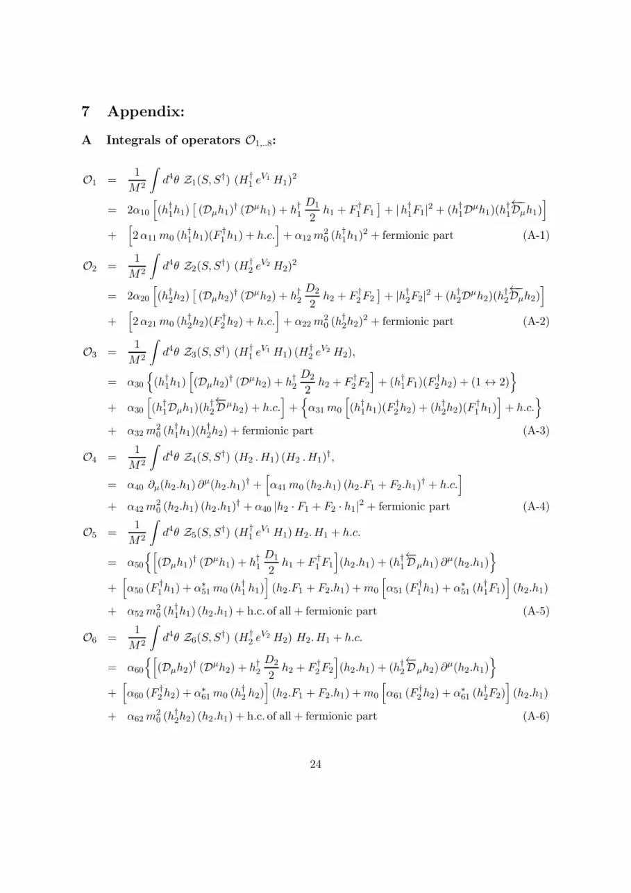
7 Appendix:
A Integrals of operators O1,..8:
O1 =1
M2
∫
d4θ Z1(S, S†) (H†
1 eV1 H1)
2
= 2α10
[
(h†1h1)[
(Dµh1)† (Dµh1) + h†1
D1
2h1 + F †
1F1
]
+ |h†1F1|2 + (h†1Dµh1)(h†1
←−Dµh1)]
+[
2α11 m0 (h†1h1)(F
†1h1) + h.c.
]
+ α12 m20 (h
†1h1)
2 + fermionic part (A-1)
O2 =1
M2
∫
d4θ Z2(S, S†) (H†
2 eV2 H2)
2
= 2α20
[
(h†2h2)[
(Dµh2)† (Dµh2) + h†2
D2
2h2 + F †
2F2
]
+ |h†2F2|2 + (h†2Dµh2)(h†2
←−Dµh2)]
+[
2α21 m0 (h†2h2)(F
†2h2) + h.c.
]
+ α22 m20 (h
†2h2)
2 + fermionic part (A-2)
O3 =1
M2
∫
d4θ Z3(S, S†) (H†
1 eV1 H1) (H
†2 e
V2 H2),
= α30
{
(h†1h1)[
(Dµh2)† (Dµh2) + h†2
D2
2h2 + F †
2F2
]
+ (h†1F1)(F†2h2) + (1↔ 2)
}
+ α30
[
(h†1Dµh1)(h†2
←−Dµh2) + h.c.]
+{
α31 m0
[
(h†1h1)(F†2h2) + (h†2h2)(F
†1h1)
]
+ h.c.}
+ α32 m20 (h
†1h1)(h
†2h2) + fermionic part (A-3)
O4 =1
M2
∫
d4θ Z4(S, S†) (H2 .H1) (H2 .H1)
†,
= α40 ∂µ(h2.h1) ∂µ(h2.h1)
† +[
α41 m0 (h2.h1) (h2.F1 + F2.h1)† + h.c.
]
+ α42 m20 (h2.h1) (h2.h1)
† + α40 |h2 · F1 + F2 · h1|2 + fermionic part (A-4)
O5 =1
M2
∫
d4θ Z5(S, S†) (H†
1 eV1 H1)H2.H1 + h.c.
= α50
{[
(Dµh1)† (Dµh1) + h†1
D1
2h1 + F †
1F1
]
(h2.h1) + (h†1←−Dµh1) ∂
µ(h2.h1)}
+[
α50 (F†1h1) + α∗
51 m0 (h†1 h1)
]
(h2.F1 + F2.h1) +m0
[
α51 (F†1h1) + α∗
51 (h†1F1)
]
(h2.h1)
+ α52 m20 (h
†1h1) (h2.h1) + h.c. of all + fermionic part (A-5)
O6 =1
M2
∫
d4θ Z6(S, S†) (H†
2 eV2 H2) H2.H1 + h.c.
= α60
{[
(Dµh2)† (Dµh2) + h†2
D2
2h2 + F †
2F2
]
(h2.h1) + (h†2←−Dµh2) ∂
µ(h2.h1)}
+[
α60 (F†2h2) + α∗
61 m0 (h†2 h2)
]
(h2.F1 + F2.h1) +m0
[
α61 (F†2h2) + α∗
61 (h†2F2)
]
(h2.h1)
+ α62 m20 (h
†2h2) (h2.h1) + h.c. of all + fermionic part (A-6)
24
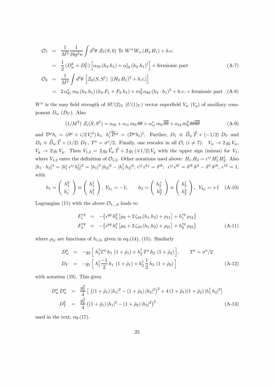
O7 =1
M2
1
16g2κ
∫
d2θ Z7(S, 0) Tr WαWα (H2 H1) + h.c.
=1
2(D2
w +D2Y )[
α70 (h2.h1) + α∗70 (h2.h1)
†]
+ fermionic part (A-7)
O8 =1
M2
∫
d4θ[
Z8(S, S†) [(H2H1)
2 + h.c.]]
= 2α∗81 m0 (h2.h1) (h2.F1 + F2.h1) +m2
0 α82 (h2 · h1)2 + h.c.+ fermionic part (A-8)
Wα is the susy field strength of SU(2)L (U(1)Y ) vector superfield Vw (Vy) of auxiliary com-
ponent Dw (DY ). Also
(1/M2) Zi(S, S†) = αi0 + αi1m0 θθ + α∗
i1 m0 θθ + αi2 m20 θθθθ (A-9)
and Dµhi = (∂µ + i/2V µi )hi, h†i
←−Dµ = (Dµhi)†. Further, D1 ≡ ~Dw
~T + (−1/2) DY and
D2 ≡ ~Dw~T + (1/2) DY , T
a = σa/2. Finally, one rescales in all Oi (i 6= 7): Vw → 2 g2 Vw,
Vy → 2 g1 Vy. Then V1,2 = 2 g2 ~Vw~T + 2 g1 (∓1/2)Vy with the upper sign (minus) for V1,
where V1,2 enter the definition of O1,2. Other notations used above: H1.H2 = ǫij H i1H
j2 . Also
|h1 · h2|2 = |hi1 ǫij hj2|2 = |h1|2 |h2|2 − |h†1 h2|2; ǫij ǫkj = δik; ǫij ǫkl = δik δjl − δil δjk, ǫ12 = 1,
with
h1 =
(
h01h−1
)
≡(
h11h21
)
, Yh1= −1; h2 =
(
h+2h02
)
≡(
h12h22
)
, Yh2= +1 (A-10)
Lagrangian (11) with the above O1,..,8 leads to
F ∗q1 = −
{
ǫqp hp2[
µ0 + 2 ζ10 (h1.h2) + ρ11]
+ h∗q1 ρ12}
F ∗q2 = −
{
ǫpq hp1[
µ0 + 2 ζ10 (h1.h2) + ρ21]
+ h∗q2 ρ22}
(A-11)
where ρij are functions of h1,2, given in eq.(14), (15). Similarly
Daw = −g2
[
h†1Ta h1 (1 + ρ1) + h†2 T
a h2 (1 + ρ2)]
, T a = σa/2
DY = −g1[
h†1−12
h1 (1 + ρ1) + h†21
2h2 (1 + ρ2)
]
(A-12)
with notation (19). This gives
Daw Da
w =g224
[ (
(1 + ρ1) |h1|2 − (1 + ρ2) |h2|2)2
+ 4 (1 + ρ1)(1 + ρ2) |h†1 h2|2]
D2Y =
g214
(
(1 + ρ1) |h1|2 − (1 + ρ2) |h2|2)2
(A-13)
used in the text, eq.(17).
25
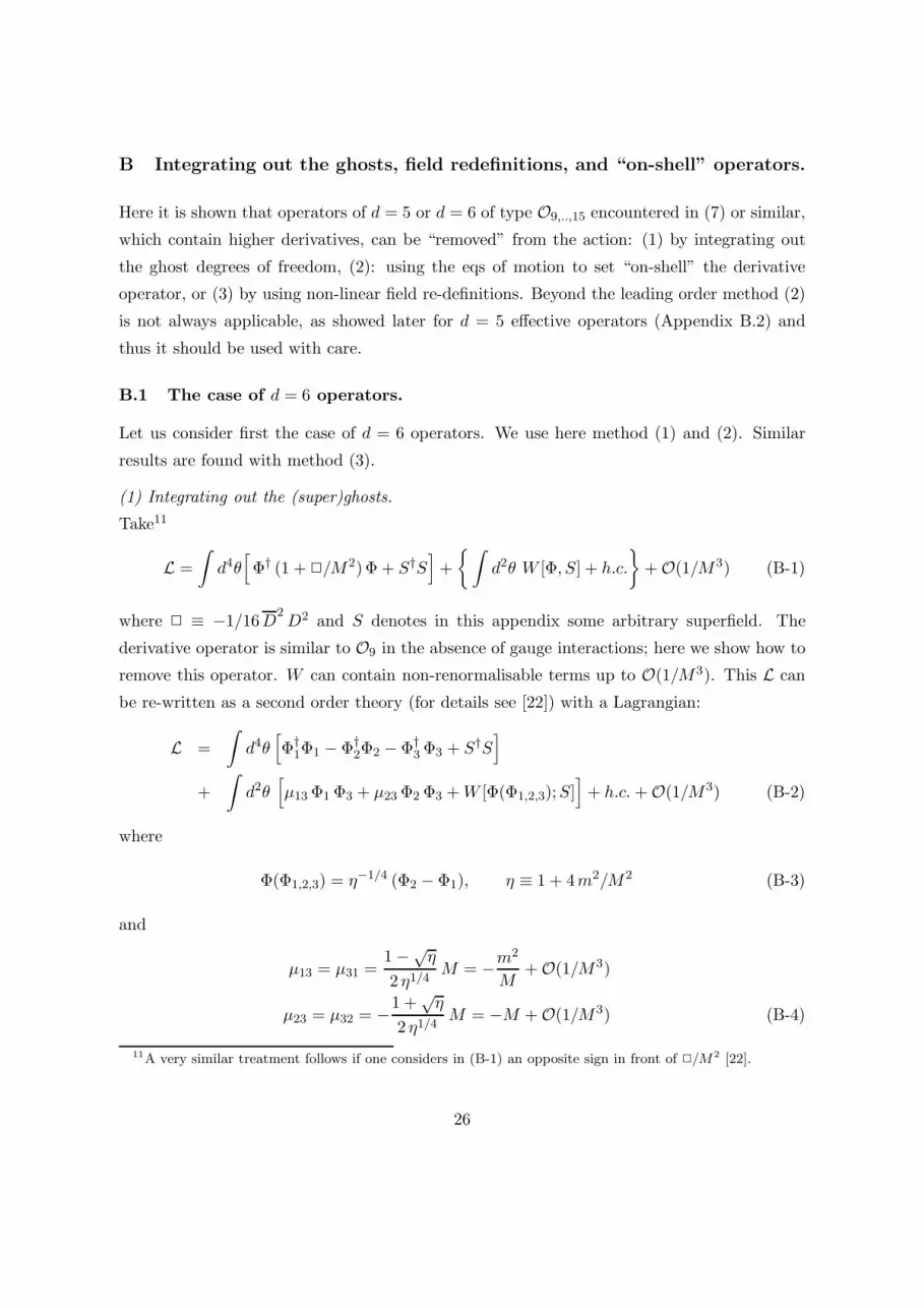
B Integrating out the ghosts, field redefinitions, and “on-shell” operators.
Here it is shown that operators of d = 5 or d = 6 of type O9,..,15 encountered in (7) or similar,
which contain higher derivatives, can be “removed” from the action: (1) by integrating out
the ghost degrees of freedom, (2): using the eqs of motion to set “on-shell” the derivative
operator, or (3) by using non-linear field re-definitions. Beyond the leading order method (2)
is not always applicable, as showed later for d = 5 effective operators (Appendix B.2) and
thus it should be used with care.
B.1 The case of d = 6 operators.
Let us consider first the case of d = 6 operators. We use here method (1) and (2). Similar
results are found with method (3).
(1) Integrating out the (super)ghosts.
Take11
L =
∫
d4θ[
Φ† (1 +2/M2)Φ + S†S]
+
{∫
d2θ W [Φ, S] + h.c.
}
+O(1/M3) (B-1)
where 2 ≡ −1/16D2D2 and S denotes in this appendix some arbitrary superfield. The
derivative operator is similar to O9 in the absence of gauge interactions; here we show how to
remove this operator. W can contain non-renormalisable terms up to O(1/M3). This L can
be re-written as a second order theory (for details see [22]) with a Lagrangian:
L =
∫
d4θ[
Φ†1Φ1 − Φ†
2Φ2 − Φ†3Φ3 + S†S
]
+
∫
d2θ[
µ13Φ1 Φ3 + µ23Φ2 Φ3 +W [Φ(Φ1,2,3);S]]
+ h.c.+O(1/M3) (B-2)
where
Φ(Φ1,2,3) = η−1/4 (Φ2 − Φ1), η ≡ 1 + 4m2/M2 (B-3)
and
µ13 = µ31 =1−√η2 η1/4
M = −m2
M+O(1/M3)
µ23 = µ32 = −1 +√η
2 η1/4M = −M +O(1/M3) (B-4)
11A very similar treatment follows if one considers in (B-1) an opposite sign in front of 2/M2 [22].
26
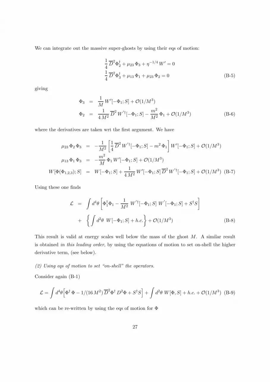
We can integrate out the massive super-ghosts by using their eqs of motion:
1
4D
2Φ†2 + µ23 Φ3 + η−1/4 W ′ = 0
1
4D
2Φ†3 + µ13 Φ1 + µ23 Φ2 = 0 (B-5)
giving
Φ3 =1
MW ′[−Φ1;S] +O(1/M3)
Φ2 =1
4M2D
2W
′†[−Φ1;S]−m2
M2Φ1 +O(1/M3) (B-6)
where the derivatives are taken wrt the first argument. We have
µ23 Φ2Φ3 = − 1
M2
[
1
4D
2W
′†[−Φ1;S]−m2Φ1
]
W ′[−Φ1;S] +O(1/M3)
µ13 Φ1Φ3 = −m2
MΦ1W
′[−Φ1;S] +O(1/M3)
W [Φ(Φ1,2,3);S] = W [−Φ1;S] +1
4M2W ′[−Φ1;S]D
2W
′†[−Φ1;S] +O(1/M3) (B-7)
Using these one finds
L =
∫
d4θ
[
Φ†1Φ1 −
1
M2W
′†[−Φ1;S] W′
[−Φ1;S] + S†S
]
+
{∫
d2θ W [−Φ1;S] + h.c.
}
+O(1/M3) (B-8)
This result is valid at energy scales well below the mass of the ghost M . A similar result
is obtained in this leading order, by using the equations of motion to set on-shell the higher
derivative term, (see below).
(2) Using eqs of motion to set “on-shell” the operators.
Consider again (B-1)
L =
∫
d4θ[
Φ†Φ− 1/(16M2)D2Φ†D2Φ+ S†S
]
+
∫
d2θ W [Φ, S] + h.c.+O(1/M3) (B-9)
which can be re-written by using the eqs of motion for Φ
27
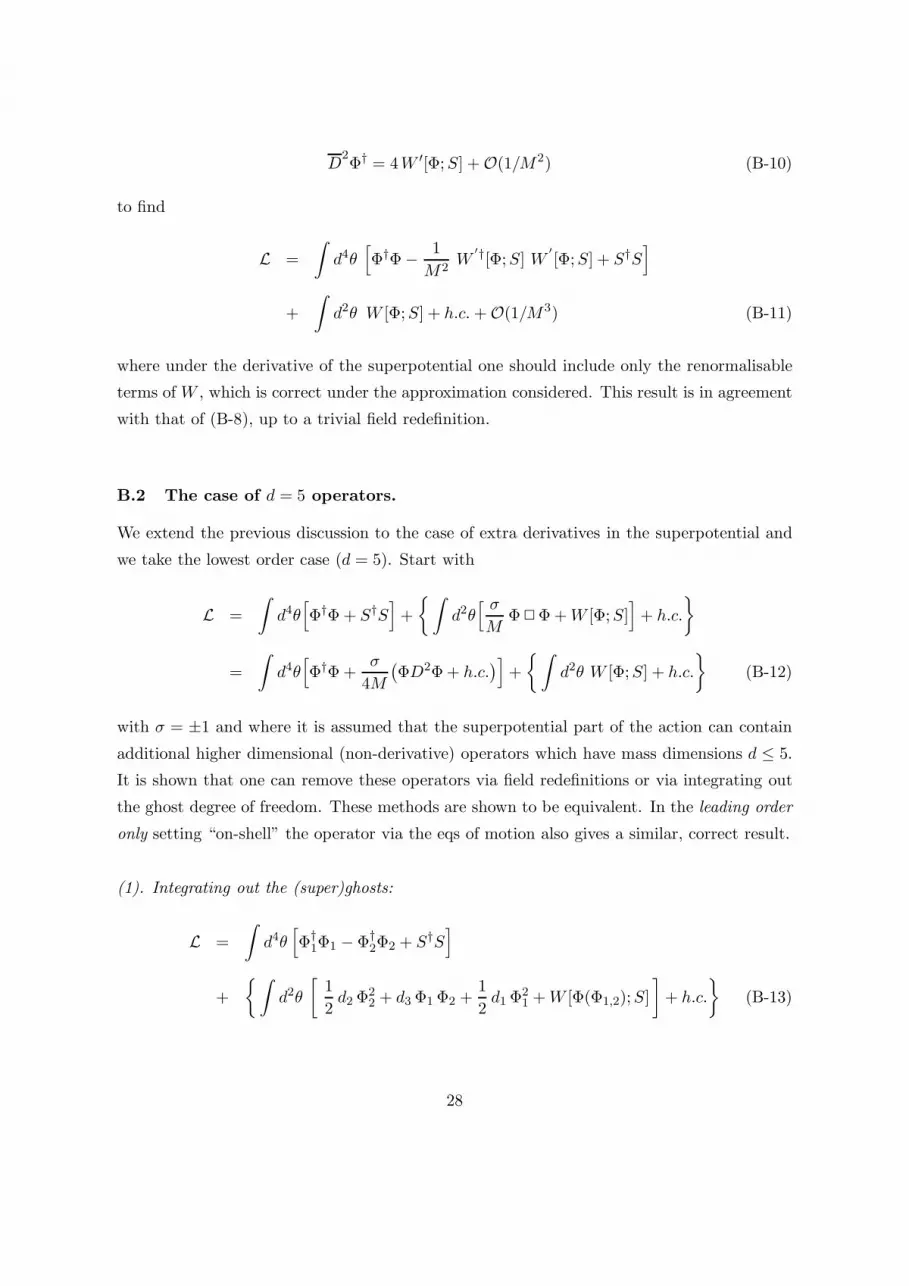
D2Φ† = 4W ′[Φ;S] +O(1/M2) (B-10)
to find
L =
∫
d4θ[
Φ†Φ− 1
M2W
′†[Φ;S] W′
[Φ;S] + S†S]
+
∫
d2θ W [Φ;S] + h.c.+O(1/M3) (B-11)
where under the derivative of the superpotential one should include only the renormalisable
terms of W , which is correct under the approximation considered. This result is in agreement
with that of (B-8), up to a trivial field redefinition.
B.2 The case of d = 5 operators.
We extend the previous discussion to the case of extra derivatives in the superpotential and
we take the lowest order case (d = 5). Start with
L =
∫
d4θ[
Φ†Φ+ S†S]
+
{∫
d2θ[ σ
MΦ2Φ+W [Φ;S]
]
+ h.c.
}
=
∫
d4θ[
Φ†Φ+σ
4M
(
ΦD2Φ+ h.c.)
]
+
{∫
d2θ W [Φ;S] + h.c.
}
(B-12)
with σ = ±1 and where it is assumed that the superpotential part of the action can contain
additional higher dimensional (non-derivative) operators which have mass dimensions d ≤ 5.
It is shown that one can remove these operators via field redefinitions or via integrating out
the ghost degree of freedom. These methods are shown to be equivalent. In the leading order
only setting “on-shell” the operator via the eqs of motion also gives a similar, correct result.
(1). Integrating out the (super)ghosts:
L =
∫
d4θ[
Φ†1Φ1 − Φ†
2Φ2 + S†S]
+
{∫
d2θ
[
1
2d2 Φ
22 + d3 Φ1Φ2 +
1
2d1 Φ
21 +W [Φ(Φ1,2);S]
]
+ h.c.
}
(B-13)
28
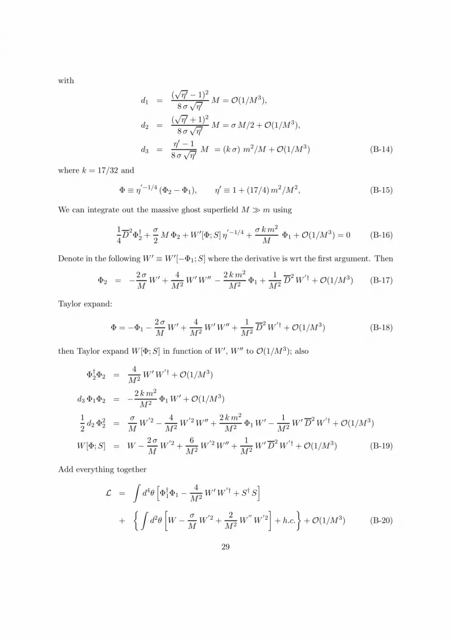
with
d1 =(√η′ − 1)2
8σ√η′
M = O(1/M3),
d2 =(√η′ + 1)2
8σ√η′
M = σM/2 +O(1/M3),
d3 =η′ − 1
8σ√η′
M = (k σ) m2/M +O(1/M3) (B-14)
where k = 17/32 and
Φ ≡ η′−1/4 (Φ2 − Φ1), η′ ≡ 1 + (17/4)m2/M2, (B-15)
We can integrate out the massive ghost superfield M ≫ m using
1
4D
2Φ†2 +
σ
2M Φ2 +W ′[Φ;S] η
′−1/4 +σ km2
MΦ1 +O(1/M3) = 0 (B-16)
Denote in the following W ′ ≡W ′[−Φ1;S] where the derivative is wrt the first argument. Then
Φ2 = −2σ
MW ′ +
4
M2W ′W ′′ − 2 km2
M2Φ1 +
1
M2D
2W
′† +O(1/M3) (B-17)
Taylor expand:
Φ = −Φ1 −2σ
MW ′ +
4
M2W ′W ′′ +
1
M2D
2W
′† +O(1/M3) (B-18)
then Taylor expand W [Φ;S] in function of W ′, W ′′ to O(1/M3); also
Φ†2Φ2 =
4
M2W ′W
′† +O(1/M3)
d3 Φ1Φ2 = −2 km2
M2Φ1 W
′ +O(1/M3)
1
2d2 Φ
22 =
σ
MW
′2 − 4
M2W
′2W ′′ +2 km2
M2Φ1 W
′ − 1
M2W ′D
2W
′† +O(1/M3)
W [Φ;S] = W − 2σ
MW
′2 +6
M2W
′2W ′′ +1
M2W ′D
2W
′† +O(1/M3) (B-19)
Add everything together
L =
∫
d4θ[
Φ†1Φ1 −
4
M2W ′W
′† + S† S]
+
{∫
d2θ
[
W − σ
MW
′2 +2
M2W
′′
W′2
]
+ h.c.
}
+O(1/M3) (B-20)
29
where the argument ofW ,W ′, W ′′ above is [−Φ1;S] and derivatives are wrt the first argument.
This is equivalent to the starting Lagrangian, with new (non-renormalisable) interactions but
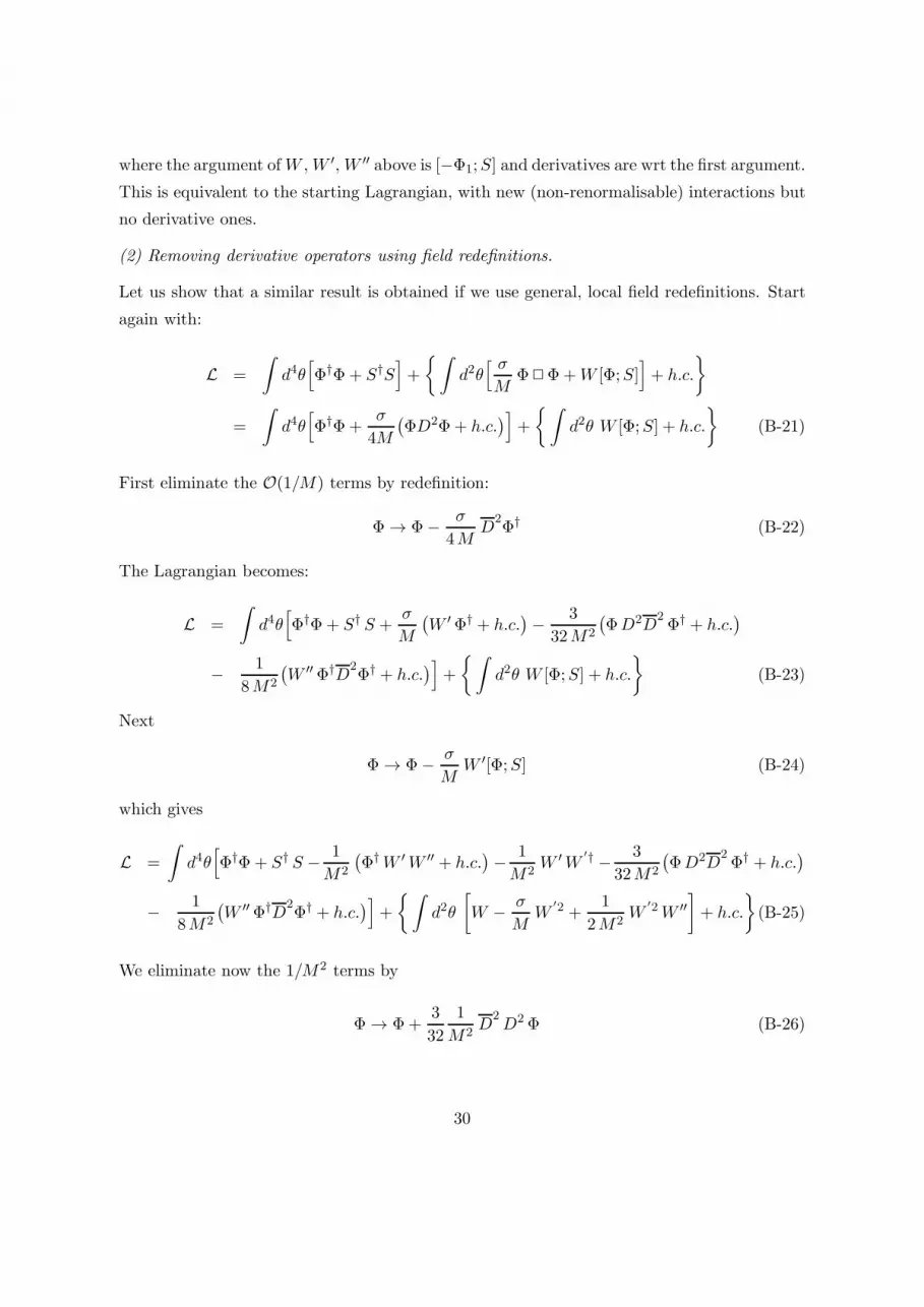
no derivative ones.
(2) Removing derivative operators using field redefinitions.
Let us show that a similar result is obtained if we use general, local field redefinitions. Start
again with:
L =
∫
d4θ[
Φ†Φ+ S†S]
+
{∫
d2θ[ σ
MΦ2Φ+W [Φ;S]
]
+ h.c.
}
=
∫
d4θ[
Φ†Φ+σ
4M
(
ΦD2Φ+ h.c.)
]
+
{∫
d2θ W [Φ;S] + h.c.
}
(B-21)
First eliminate the O(1/M) terms by redefinition:
Φ→ Φ− σ
4MD
2Φ† (B-22)
The Lagrangian becomes:
L =
∫
d4θ[
Φ†Φ+ S† S +σ
M
(
W ′Φ† + h.c.)
− 3
32M2
(
ΦD2D2Φ† + h.c.
)
− 1
8M2
(
W ′′Φ†D2Φ† + h.c.
)
]
+
{∫
d2θ W [Φ;S] + h.c.
}
(B-23)
Next
Φ→ Φ− σ
MW ′[Φ;S] (B-24)
which gives
L =
∫
d4θ[
Φ†Φ+ S† S − 1
M2
(
Φ†W ′W ′′ + h.c.)
− 1
M2W ′W
′† − 3
32M2
(
ΦD2D2Φ† + h.c.
)
− 1
8M2
(
W ′′Φ†D2Φ† + h.c.
)
]
+
{∫
d2θ
[
W − σ
MW
′2 +1
2M2W
′2W ′′]
+ h.c.
}
(B-25)
We eliminate now the 1/M2 terms by
Φ→ Φ+3
32
1
M2D
2D2Φ (B-26)
30

giving
L =
∫
d4θ[
Φ†Φ+ S† S − 1
M2
(
Φ†W ′W ′′ + h.c.)
− 1
M2W ′W
′† − 3
8M2(W ′D2Φ+ h.c.)
− 1
8M2
(
W ′′Φ†D2Φ† + h.c.
)
]
+
{∫
d2θ
[
W − σ
MW
′2 +1
2M2W
′2W ′′]
+ h.c.
}
(B-27)
Next consider
Φ→ Φ+1
8M2W ′′D
2Φ† (B-28)
to find
L =
∫
d4θ[
Φ†Φ+ S† S − 3
2M2
(
Φ†W ′W ′′ + h.c.)
− 1
M2W ′W
′† − 3
8M2(W ′D2Φ+ h.c.)
]
+
{∫
d2θ
[
W − σ
MW
′2 +1
2M2W
′2 W ′′]
+ h.c.
}
(B-29)
then
Φ→ Φ+3
8M2D
2W
′†[Φ;S] (B-30)
to obtain
L =
∫
d4θ[
Φ†Φ+ S† S − 3
2M2
(
Φ†W ′W ′′ + h.c.)
− 1
M2W ′W
′†]
+
{∫
d2θ
[
W − σ
MW
′2 +1
2M2W
′2 W ′′ +3
8M2W ′D
2W
′†]
+ h.c.
}
(B-31)
Finally
Φ→ Φ+3
2M2W ′[Φ;S]W ′′[Φ;S] (B-32)
one finds
L =
∫
d4θ[
Φ†Φ+ S† S − 4
M2W ′W
′†]
+
{∫
d2θ
[
W − σ
MW
′2 +2
M2W
′2W ′′]
+ h.c.
}
(B-33)
which agrees with the result in (B-20) up to and including O(1/M2) terms.
31
(3) Setting “on-shell” the derivative operators by using the eqs of motion.
Let us discuss what happens if in action (B-12) we “removed” the higher derivative terms
by using the equations of motion i.e. setting them “on-shell”. It will turn out that only in
leading order (1/M) do we obtain a similar L as in previous cases. The eq of motion is
D2Φ† = 4W ′ +O(1/M) (B-34)
where W ′ ≡ ∂W [Φ;S]/∂Φ. This is used in (B-12), and after an additional shift to re-write
higher dimensional D-terms as F-terms
Φ→ Φ− (σ/M)W ′ (B-35)
we obtain:
L =
∫
d4θ[
Φ†Φ+ S†S]
+
{∫
d2θ W [Φ− (σ/M) W ′; S] + h.c.
}
=
∫
d4θ[
Φ†Φ+ S†S]
+
{∫
d2θ[
W [Φ;S]− (σ/M) W ′2[Φ;S]]
+ h.c.
}
(B-36)
where we used a Taylor expansion in the last step. If we include the next order, after using
D2Φ† = 4W ′ − σ
MD
2W
′† +O(1/M2) (B-37)
and after the following redefinitions
Φ→ Φ− σ
MW ′ (B-38)
and
Φ→ Φ+1
M2W ′W ′′ (B-39)
one finds
L=∫
d4θ[
Φ†Φ+ S† S − 3
M2W ′W
′†]
+
{∫
d2θ
[
W− σ
MW
′2+3
2M2W
′2W ′′]
+ h.c.
}
(B-40)
Although this agrees with (B-20) in O(1/M), it disagrees with it in order O(1/M2). The
reason for this is that the “on-shell” setting method of higher dimensional operators is derived
using general field redefinitions only in the leading order O(1/M). As a result this method
should be used with care.
32
C Coefficients for the Higgs masses.
The coefficients in eq.(36) have the following expressions:
γ±1 =±v2
2u2(1 + u2)3 w1/2
×[
(B0m0µ0)2 (1 + u2)4 − 2m2
Z u2[
m2Z(1− u2)2 + (1 + u2) (8µ2
0 u2 ± (u2 − 1)w1/2))
]
+ (B0m0µ0)u(1 + u2)2[
m2Z (1 + u2)− (±w1/2(1 + u2) + 16µ2
0 u2)]
]
(C-1)
γ±2 =±v2
2(1 + u2)3 w1/2
×[
(B0m0µ0)2(1 + u2)4 − 2m2
Zu2[
8µ20(1 + u2) +m2
Z(1− u2)2 ± w1/2(1− u4)]
− (B0m0µ0)u (1 + u2)2[
16µ20 −m2
Z(1 + u2)± (1 + u2)w1/2]
]
(C-2)
γ±3 = γ±4 =±v2
u (1 + u2)2 w1/2
{
µ20
[
−B0m0µ0 (1+u2)3+m2Zu(1−6u2+ u4)∓ u(1+u2)2 w1/2
]
+ B0m0µ0 u2 (1 + u2)m2
Z +m2Z u3 (m2
Z ∓ w1/2)}
(C-3)
γ±5 =∓v2
8u3 (1 + u2)3 w1/2
[
(B0m0µ0)2(1 + u2)4 (−1 + 3u2)− (B0m0µ0)u(1 + u2)2
×[
− 2m2Z(1 + 5u2) + 2µ2
0 (1 + 8u2 + 25u4 + 2u6)± (1 + u2)(3u2 − 1)w1/2]
− u2m2Z
[
m2Z(1− 19u2 − u4 + 3u6)− 2µ2
0 (1 + u2)(1− 16u2 − 23u4 + 2u6)
± (1 + u2)2(1 + 3u2)w1/2]
+ 2µ20 u
2[
± (1 + u2)2 (1− 9u2 + 2u4)w1/2]
]
(C-4)
γ±6 =±v2
8u2 (1 + u2)3 w1/2
[
(B0m0µ0)2 u (1 + u2)4 (−3 + u2)− (B0m0µ0) (1 + u2)2
×[
2m2Z(5 + u2)u4 − 2µ2
0 (2 + 25u2 + 8u4 + u6)± (1 + u2) (u2 − 3)u2 w1/2]
+ um2Z
[
m2Z(3− u2 − 19u4 + u6)u2 − 2µ2
0 (1 + u2)(2 − 23u2 − 16u4 + u6)
± u2 (1 + u2)2(3 + u2)w1/2]
− 2µ20 u[
± (1 + u2)2 (2− 9u2 + u4)w1/2]
]
(C-5)
γ±7 =∓v2m2
Z
16u2(1 + u2)3 w1/2
[
−B0m0µ0 (1 + u2)(1 + 40u2 − 114u4 + 40u6 + u8)
+ m2Z (u+ 30u5 + u9)± u(1 + u2)2(1− 10u2 + u4)w1/2
]
(C-6)
γ±x =±8 (u2 − 1)2 v4
u (1 + u2)3 w3/2
[
m2Z u−B0m0µ0 (1 + u2)
][
2m2Z u−B0m0µ0 (1 + u2)
]
m0 µ0 (C-7)
γ±y = ∓ (−1 + u2)2 v4
(1 + u2)4 w3/2
[
m2Z u−B0 m0 µ0 (1 + u2)
]2(4m2
0) (C-8)
33
γ±z =∓v4
µ20 u
2 (1 + u2)3 w3/2(C-9)
×[
− 2 (B0m0µ0)3 u (1 + u2)4 +m4
Z u2(1 + u2)(
4µ20(−1 + u2)2 − u2(2m2
Z ± w1/2))
+ 2B0m0µ0m2Z u[
− 2µ20(u
4 − 1)2 + u2(m2Z(1− 14u2 + u4)± (u4 − 6u2 + 1)w1/2)
]
+ (B0m0µ0)2 (1 + u2)
[
µ20 (u
4 − 1)2 + u2(2m2Z (1− 14u2 + u4)∓ (1 + u2)2 w1/2)
]
]
(4µ20)
D One-loop mh with d = 5 operators
For future reference, it is worth mentioning the value of mh in the presence of one-loop
corrections from top-stop and d = 5 operators [16], mentioned in the text:
m2h =
1
2
[
m′ 2A +m2
Z −√w′ + ξ
]
+ (2 ζ10 µ0) v2 sin 2β
[
1 +m
′ 2A +m2
Z√w′
]
+(−2 ζ11 m0) v2
2
[
1− (m′ 2A −m2
Z) cos2 2β√
w′
]
(D-1)
where
w′ ≡ [(m
′ 2A −m2
Z) cos 2β + ξ]2 + sin2 2β (m′ 2A +m2
Z)2
m′ 2A = m2
1 + m22 + ξ/2 + (2 ζ10µ0) v
2 sin 2β + ζ11 m0 v2; ξ ≡ δ m2
Z sin2 β (D-2)
where δ is the one-loop correction from top-stop Yukawa sector to λ02 of (27) which changes
according to λ02 → λ0
2 (1 + δ) where [7, 24]
δ =3h4tg2 π2
[
lnMt
mt+
Xt
4+
1
32π2
(
3h2t − 16 g23
)(
Xt + 2 lnMt
mt
)
lnMt
mt
]
,
Xt ≡2 (At m0 − µ cot β)2
M2t
[
1− (Atm0 − µ cot β)2
12 M2t
]
. (D-3)
with M2t≡ mt1
mt2, and g3 the QCD coupling. The combined effect of d = 5 operators and
top Yukawa coupling ht is that mh can reach values of 130 GeV for tan β ≤ 7 with a small
fine-tuning ∆ ≤ 10 [16] and with the supersymmetric coefficient ζ10 giving a larger effect
than the non-susy one, ζ11. Even for a modest increase of mh from d = 5 operators alone of
order O(10GeV ), their impact on the effective quartic coupling of the Higgs field is significant
(due to the small value of the MSSM gauge couplings), and this explains the reduction of
fine-tuning by the effective operators.
34
References
[1] R. Barate et al. [LEP Working Group for Higgs boson searches], “Search for the stan-
dard model Higgs boson at LEP,” Phys. Lett. B 565, 61 (2003) [arXiv:hep-ex/0306033];
S. Schael et al. [ALEPH Collaboration], “Search for neutral MSSM Higgs bosons at LEP,”
Eur. Phys. J. C 47, 547 (2006) [arXiv:hep-ex/0602042].
[2] S. S. AbdusSalam, B. C. Allanach, F. Quevedo, F. Feroz and M. Hobson, “Fitting the
Phenomenological MSSM,” arXiv:0904.2548 [hep-ph].
[3] R. Barbieri and A. Strumia, “About the fine-tuning price of LEP,” Phys. Lett. B 433
(1998) 63 [arXiv:hep-ph/9801353].
[4] P. H. Chankowski, J. R. Ellis, M. Olechowski and S. Pokorski, “Haggling over the fine-
tuning price of LEP,” Nucl. Phys. B 544 (1999) 39 [arXiv:hep-ph/9808275].
[5] P. H. Chankowski, J. R. Ellis and S. Pokorski, “The fine-tuning price of LEP,” Phys.
Lett. B 423 (1998) 327 [arXiv:hep-ph/9712234].
[6] G. L. Kane and S. F. King, “Naturalness implications of LEP results,” Phys. Lett. B
451 (1999) 113 [arXiv:hep-ph/9810374].
[7] G. F. Giudice and R. Rattazzi, “Living dangerously with low-energy supersymmetry,”
Nucl. Phys. B 757 (2006) 19 [arXiv:hep-ph/0606105].
[8] G. F. Giudice, C. Grojean, A. Pomarol and R. Rattazzi, “The Strongly-Interacting Light
Higgs,” JHEP 0706 (2007) 045 [arXiv:hep-ph/0703164].
[9] M. Dine, N. Seiberg and S. Thomas, “Higgs Physics as a Window Beyond the MSSM
(BMSSM),” Phys. Rev. D 76 (2007) 095004 [arXiv:0707.0005 [hep-ph]].
[10] I. Antoniadis, E. Dudas, D. M. Ghilencea and P. Tziveloglou, “MSSM with Dimension-
five Operators (MSSM5),” Nucl. Phys. B 808 (2009) 155 [arXiv:0806.3778 [hep-ph]].
[11] I. Antoniadis, E. Dudas, D. M. Ghilencea and P. Tziveloglou, “Higher Dimensional Op-
erators in the MSSM,” AIP Conf. Proc. 1078 (2009) 175 [arXiv:0809.4598 [hep-ph]].
[12] K. Blum, C. Delaunay and Y. Hochberg, “Vacuum (Meta)Stability Beyond the MSSM,”
arXiv:0905.1701 [hep-ph].
35
[13] M. Berg, J. Edsjo, P. Gondolo, E. Lundstrom and S. Sjors, “Neutralino Dark Matter in
BMSSM Effective Theory,” arXiv:0906.0583 [hep-ph].
[14] K. Blum and Y. Nir, “Beyond MSSM Baryogenesis,” Phys. Rev. D 78 (2008) 035005
[arXiv:0805.0097 [hep-ph]].
[15] S. W. Ham, S. a. Shim and S. K. OH, “Possibility of spontaneous CP violation in Higgs
physics beyond the minimal supersymmetric standard model,” arXiv:0907.3300 [hep-ph].
[16] S. Cassel, D. M. Ghilencea and G. G. Ross, “Fine tuning as an indication of physics
beyond the MSSM,” Nucl. Phys. B 825 (2010) 203 [arXiv:0903.1115 [hep-ph]].
[17] P. Batra, A. Delgado, D. E. Kaplan and T. M. P. Tait, “The Higgs mass bound in
gauge extensions of the minimal supersymmetric standard model,” JHEP 0402 (2004)
043 [arXiv:hep-ph/0309149].
[18] R. Barbieri and G. F. Giudice, “Upper Bounds On Supersymmetric Particle Masses,”
Nucl. Phys. B 306 (1988) 63;
[19] H. Georgi, “On-Shell Effective Field Theory,” Nucl. Phys. B 361 (1991) 339.
[20] H. D. Politzer, “Power Corrections At Short Distances,” Nucl. Phys. B 172 (1980) 349.
[21] C. Arzt, “Reduced effective Lagrangians,” Phys. Lett. B 342 (1995) 189
[arXiv:hep-ph/9304230].
[22] I. Antoniadis, E. Dudas and D. M. Ghilencea, “Supersymmetric Models with Higher
Dimensional Operators,” JHEP 0803 (2008) 045 [arXiv:0708.0383 [hep-th]].
[23] D. Piriz and J. Wudka, “Effective operators in supersymmetry,” Phys. Rev. D 56 (1997)
4170 [arXiv:hep-ph/9707314].
[24] M. S. Carena, J. R. Espinosa, M. Quiros and C. E. M. Wagner, “Analytical expressions
for radiatively corrected Higgs masses and couplings in the MSSM,” Phys. Lett. B 355
(1995) 209 [arXiv:hep-ph/9504316].
[25] S. Cassel, D. M. Ghilencea, G. G. Ross, work in progress.
[26] A. Brignole, J. A. Casas, J. R. Espinosa and I. Navarro, “Low-scale supersymmetry
breaking: Effective description, electroweak breaking and phenomenology,” Nucl. Phys.
B 666 (2003) 105 [arXiv:hep-ph/0301121].
36
[27] J. R. Espinosa and M. Quiros, “On Higgs Boson Masses In Nonminimal Supersymmetric
Standard Models,” Phys. Lett. B 279 (1992) 92.
[28] J. R. Espinosa and M. Quiros, “Gauge unification and the supersymmetric light Higgs
mass,” Phys. Rev. Lett. 81 (1998) 516 [arXiv:hep-ph/9804235].
[29] J. R. Espinosa and M. Quiros, “Higgs boson bounds in nonminimal supersymmetric
standard models,” arXiv:hep-ph/9208226.
[30] J. R. Espinosa and M. Quiros, “Upper bounds on the lightest Higgs boson mass in general
supersymmetric Standard Models,” Phys. Lett. B 302 (1993) 51 [arXiv:hep-ph/9212305].
[31] M. Carena, K. Kong, E. Ponton and J. Zurita, “Supersymmetric Higgs Bosons and
Beyond,” arXiv:0909.5434 [hep-ph].
37