MS -Excel 97

explained

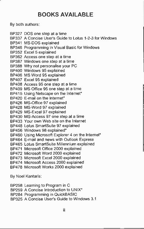
BOOKS AVAILABLE

By both authors:

BP327 DOS one step at a timeBP337 A Concise User's Guide to Lotus 1-2-3 for WindowsBP341 MS-DOS explainedBP346 Programming in Visual Basic for WindowsBP352 Excel 5 explainedBP362 Access one step at a timeBP387 Windows one step at a timeBP388 Why not personalise your PCBP400 Windows 95 explainedBP406 MS Word 95 explainedBP407 Excel 95 explainedBP408 Access 95 one step at a timeBP409 MS Office 95 one step at a timeBP415 Using Netscape on the Internet*BP420 E-mail on the Internet*BP426 MS -Office 97 explainedBP428 MS -Word 97 explainedBP429 MS -Excel 97 explainedBP430 MS -Access 97 one step at a timeBP433 Your own Web site on the InternetBP448 Lotus SmartSuite 97 explainedBP456 Windows 98 explained*BP460 Using Microsoft Explorer 4 on the Internet*BP464 E-mail and news with Outlook ExpressBP465 Lotus SmartSuite Millennium explainedBP471 Microsoft Office 2000 explainedBP472 Microsoft Word 2000 explainedBP473 Microsoft Excel 2000 explainedBP474 Microsoft Access 2000 explainedBP478 Microsoft Works 2000 explained

By Noel Kantaris:

BP258 Learning to Program in CBP259 A Concise Introduction to UNIX*BP284 Programming in QuickBASICBP325 A Concise User's Guide to Windows 3.1

II

MS -Excel 97explained

by

N. Kantarisand

P.R.M. Oliver

BERNARD BABANI (publishing) LTD.THE GRAMPIANS

SHEPHERDS BUSH ROADLONDON W6 7NF

ENGLAND

PLEASE NOTE

Although every care has been taken with theproduction of this book to ensure that any projects,designs, modifications and/or programs, etc.,contained herewith, operate in a correct and safemanner and also that any components soecified arenormally available in Great Britain, the Publishers andAuthor(s) do not accept responsibility in any way forthe failure (including fault in design) of any project,design, modification or program to work correctly or tocause damage to any equipment that it may beconnected to or used in conjunction with, or in respectof any other damage or injury that may be so caused,nor do the Publishers accept responsibility in any wayfor the failure to obtain specified components.

Notice is also given that if equipment that is stillunder warranty is modified in any way or used orconnected with home -built equipment then thatwarranty may be void

© 1997 BERNARD BABANI (publishing) LTD

First published - September 1997Reprinted - November 1998Reprinted - October 1999

British Library Cataloguing in Publication Data:A catalogue record for this book is available from the British Library

ISBN 0 85934 429 0

Cover Design by Gregor Arthur

Cover illustration by Adam Willis

Printed and bound in Great Britain by Cox & Wyman Ltd, Reading

ABOUT THIS BOOK

MS -Excel 97 explained has been written for those whowant to get to grips with the latest 3 -dimensionalspreadsheet for Windows 95 from Microsoft, in thefastest possible time. The material in this book ispresented on the 'what you need to know first, appearsfirst' basis, although the underlying structure is suchthat slightly more experienced users need not star. atthe beginning and go right through to the end; they canstart from any secticn, as each section of the book hasbeen designed to be self contained.

No previous knowledge of spreadsheets is assumed,so that users without any knowledge of the subject canfollow the book easily, but we do not describe how toset up your computer hardware, or how to install anduse Windows 95. If you need to know more about theWindows environment, then may we suggest youselect an appropriate level book for your needs fromthe 'Books Available' list - the books are graduated incomplexity with the less demanding One step at a timeseries, to the more detailed Explained series. They areall published by BERNARD BABANI (publishing) Ltd.

Microsoft Excel 97 is a very powerful spreadsheetpackage that has the ability to work 3-dimeisiorallywith both multiple worksheets and files. It is operatedby selecting commands from drop -down menus, byusing buttons, or by writing 'macros' to chain togethermenu commands. Each method of accessing thepackage is discussed separately, but the emphasis ismostly in the area of menu -driven and button clickingcommand selection. Working under the Windows 95environment, gives the package an excellentWYSIWYG (What You See Is What You Get)appearance which, it turn, allows for the productio-i ofhighly professional quality printed material.

Most features of the package will be discussed usingsimple examples that the user is encouraged to type in,save, and modify as more advanced features areintroduced. This provides the new user with a set ofexamples that aim to help with the learning process,and should help to provide the confidence needed totackle some of the more advanced capabilities of thepackage later.

For those who would like to practise with additionalexamples, slightly unguided, but with enoughinstruction so that they can be completed successfully,we have included three exercises in the penultimatechapter of the book. The exercises are drawn fromsufficiently general topics, so as to maximise theirsuitability to your needs and understanding.

Although the book is intended as a supplement tothe 'Help' documentation that comes with the package,in the last chapter of the book, all the Excel 97functions are listed so that it is self contained and canbe used as a reference long after you become anexpert in the use of the program.

If you would like to purchase a Companion Disc for any cf the listed booksby the same author(s), apart from the ones marked with an asterisk,containing the file/program listings which appear in them, hen fill in the format the back of the book and send it to Phil Oliver at the stipulated address.

ABOUT THE AUTHORS

Noel Kantaris graduated in Electrical Engineering at BristolUniversity and after spending three years in the ElectronicsIndustry in London, took up a Tutorship in Physics at theUniversity of Queensland. Research interests in IonosphericPhysics, led to the degrees of M.E. in Electronics and Ph.D.in Physics. On return to the UK, he took up a Post -DoctoralResearch Fellowship in Radio Physics at the University ofLeicester, and then in 1973 a lecturing position inEngineering at the Camborne School of Mines, Cornwall,(part of Exeter University), where between 1978 and 1997 hewas also the CSM Computing Manager. At present he is ITDirector of FFC Ltd.

Phil Oliver graduated in Mining Engineering at CamborneSchool of Mines in 1967 and since then has specialised inmost aspects of surface mining technology, with a particularemphasis on computer related techniques. He has worked inGuyana, Canada, several Middle Eastern countries, ScuthAfrica and the United Kingdom, on such diverse projects as:the planning and management of bauxite,mines; rock excavation contracting in the UK; internationalmining equipment sales and international mine consulting fora major mining house in South Africa. In 1988 he took Lp alecturing position at Camborne School of Mines (par. ofExeter University) in Surface Mining and Management. Heretired from full-time lecturing in 1998, to spend more timewriting, consulting and developing Web sites for clients.

vii

OF'

ACKNOWLEDGEMENTS

We would like to thank the staff of Text 100 Limited forproviding the software programs on which this workwas based. We would also like to thank colleagues atthe Camborne School of Mines for the helpful tips andsuggestions which assisted us in the writing of thisbook.

L

TRADEMARKS

Arial and Times New Roman are regis:eredtrademarks of The Monotype Corporation plc.

HP and LaserJet are registered trademarks of HewlettPackard Corporation.

IBM is a registered trademark of International BusinessMachines, Inc.

Intel is a registered trademark of Intel Corporation.

Lotus, 1-2-3 is a registered trademark of LotusDevelopment Corporation.

Microsoft, MS-DOS, Windows, Windows NT, Works,and Visual Basic, are either registered trademarks ortrademarks of Microsoft Corporaticn.

PostScript is a registered trademark of AdobeSystems Incorporated.

TrueType is a registered trademark of AppleCorporation.

All other brand and product names used in the book arerecognised as trademarks, or registered trademarks, of theirrespective companies.

CONTENTS

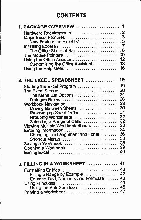
1 PACKAGE OVERVIEW 1

Hardware Requirements 2

Major Excel Features 3

New Features in Excel 97 5

Installing Excel 97 7

The Office Shortcut Bar 8The Mouse Pointers 10Using the Office Assistant 12

Customising the Office Assistant 13Using the Help Menu 16

2. THE EXCEL SPEADSHEET 19

Starting the Excel Program 19The Excel Screen 20

The Menu Bar Options 24Dialogue Boxes 26

Workbook Navigation 28Moving Between Sheets 30Rearranging Sheet Order 31

Grouping Worksheets 32Selecting a Range of Cells 32

Viewing Multiple Workbook Sheets 33Entering Information 34

Changing Text Alignment and Fonts 36Shortcut Mends 38

Saving a Workbook 38Opening a Work000k 39Exiting Excel 40

3. FILLING IN A WORKSHEET 41

Formatting Entries 42Filling a Range by Example ......... 42Entering Text, Numbers and Formulae .. 43

Using Functions 43Using the AutoSum Icon 45

Printing a Worksheet 47

Enhancing a Worksheet 49Header and Footer Icons and Codes 50Setting a Print Area 51

3 -Dimensional Worksheets 53Manipulating Ranges 53Copying Sheets into a Workbook 53

Linking Sheets 56Linking Files 57

File Commands 57Relative and Absolute Cell Addresses 60Freezing Panes on Screen 61

4. SPREADSHEET CHARTS 63

Preparing for a Column Chart 63The Chart Wizard 65

Editing a Chart 69Saving Charts 69

Pre -defined Chart Types 70Customising a Chart 72

Drawing a Multiple Column Chart 72Changing a Title and an Axis Label 73Drawing a Pie Chart 75

The Drawing Tools 78Office Art 79Creating a Drawing 80Editing a Chart 80

5. THE EXCEL DATABASE 81

Creating a Database 82Sorting a Database List 85

Date Arithmetic 86The IF Function 87Searching a Database 89

Using the Database Form 89Finding Records 91

Extracting Records 94Structuring a Workbook 95

6. OTHER TOOLS AND CAPABILITIES 99

The Auditor 99The Goal Seek 101What -if Tables 102

A Two -Input What -if Table 103Editing a Data Table 105

The Solver 106Starting the Solver 107Entering Constraints 108Solving a Problem 108

Managing Wha:-if Scenarios 110

7. SHARING INFORMATION 113

Copying or Moving Information 114Source File Available without Application 114Source File and Application Available 116

Inserting an Excel Worksheet in Word 97 118Object Linking and Embedding 119

Embedding a New Object 120Linking or Embedding an Existing File 122Editing an Embedded Object 124

Hyperlinks 126

8. USING MACROS 129

Using the Mac -c Recorder 130Recording an Excel 97 Macro ....... 131

Programming Advantages with Visual Basic 134Reading Visual Basic Code 134

Editing a Macro 136Macro Interaction with Keyboard 138

9. EXERCISES USING EXCEL 97 141

Compound Interest 141

Product Sales Calculations 143Salary Calculations 145

10. FUNCTIONS 147Types of Functions 147

Financial Functions 149Date and Time Functions 151Mathematical and Trigonometric -Functions 152Statistical Functions 156Lookup and Reference Functions 162Database Functions 164Text Functions 165Logical Functions 167Information Functions 168

INDEX 169

1. PACKAGE OVERVIEW

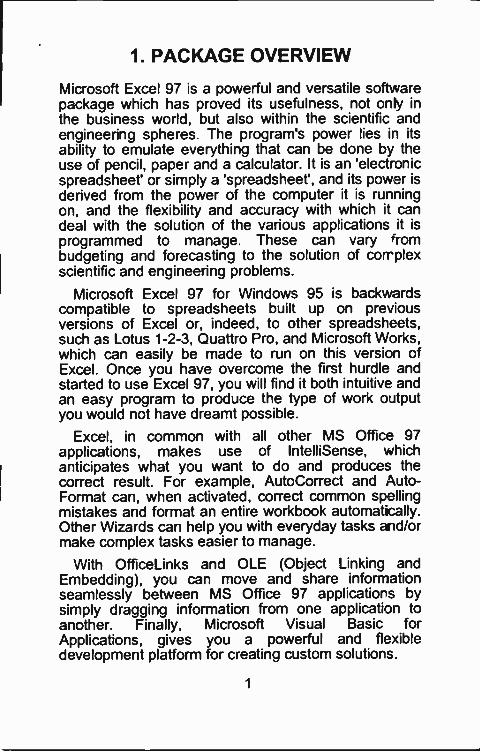
Microsoft Excel 97 is a powerful and versatile softwarepackage which has proved its usefulness, not only inthe business world, but also within the scientific andengineering spheres The program's power lies in itsability to emulate everything that can be done by theuse of pencil, paper and a calculator. It is an 'electronicspreadsheet' or simply a 'spreadsheet', and its power isderived from the power of the computer it is runningon, and the flexibility and accuracy with which it candeal with the solution of the various applications it is

programmed to manage. These can vary 'rambudgeting and forecasting to the solution of complexscientific and engineering problems.

Microsoft Excel 97 for Windows 95 is backwardscompatible to spreadsheets buil'. up on previousversions of Excel or, indeed, to other spreadsheets,such as Lotus 1-2-3, Quattro Pro, and Microsoft Works,which can easily be made to run on this versicn ofExcel. Once you have overcome the first hurdle andstarted to use Excel 97, you will find it both intuitive andan easy program to produce the type of work oJtputyou would not have dreamt possible.

Excel, in common with all other MS Office 97applications, makes use of IntelliSense, whichanticipates what you want to do and produces thecorrect result. For example, AutoCorrect and Auto -Format can, when activated, correct commcn spellingmistakes and format an entire workbook automatically.Other Wizards can help you with everyday tasks and/ormake complex tasks easier to manage.

With OfficeLinks and OLE (Object Linking andEmbedding), you can move and share informationseamlessly between MS Office 97 applicatiors bysimply dragging information from one application toanother. Finally, Microsoft Visual Basic forApplications, gives you a powerful and flexibledevelopment platform for creating custom soiutiors.

1

Hardware Requirements

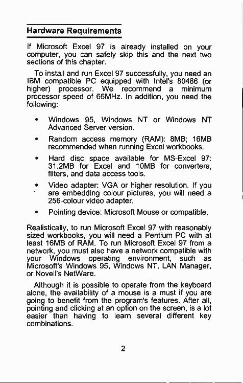
If Microsoft Excel 97 is already installed on yourcomputer, you can safely skip this and -.he next twosections of this chapter.

To install and run Excel 97 successfully, you need anIBM compatible PC equipped with Intel's 80486 (orhigher) processor. We recommend a minimumprocessor speed of 66MHz. In addition, you need thefollowing:

Windows 95, Windows NT or Windows NTAdvanced Server version.

Random access memory (RAM): 8MB; 16MBrecommended when running Excel workbooks.

Hard disc space available for MS -Excel 97:31.2MB for Excel and 10MB for converters,filters, and data access tools.

Video adapter: VGA or higher resolution. If youare embedding colour pictures, you will need a256 -colour video adapter.

Pointing device: Microsoft Mouse or compatible.

Realistically, to run Microsoft Excel 97 with reasonablysized workbooks, you will need a Pentium PC with atleast 16MB of RAM. To run Microsoft Excel 97 from anetwork, you must also have a network compatible withyour Windows operating environment, such asMicrosoft's Windows 95, Windows NT, LAN Manager,or Novell's NetWare.

Although it is possible to operate from the keyboardalone, the availability of a mouse is a must if you aregoing to benefit from the program's features. After all,pointing and clicking at an option on the screen, is a loteasier than having to learn several different keycombinations.

2

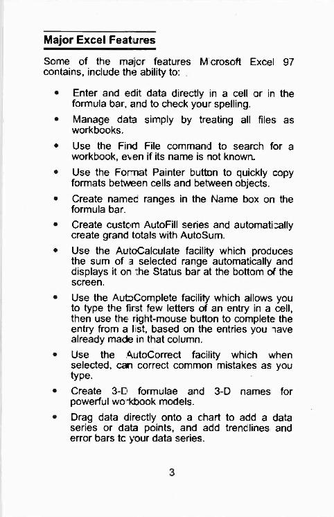
Major Excel Features

Some of the majcr features M crosoft Excel 97contains, include the ability to:

Enter and edif. data directly in a cell r in theformula bar, and to check you- spelling.

Manage data simply by treating all files asworkbooks.

Use the Find File command to search for aworkbook, e%en if its name is got known.

Use the Format Painter button to quickly copyformats between cells and between objects.

Create namec ranges in the Name box on theformula bar.

Create custom AutoFill series and automatballycreate grand totals with AutoSum.

Use the Au:oCalculate facility which producesrange automatically and

displays it on The Status bar at the bottpm of thescreen.

Use the AubComplete facility which allows youto type the first few letters of an entry in a cell,then use the right -mouse button to complete theentry from a I st, based on the entries you lavealready macie in that column.

Use the 4utoCorrect facility which whenselected, can correct common mistakes as youtype.

Create 3-E, formulae and 3-D names forpowerful wolcbook models.

Drag data directly onto a chart to add a dataseries or data points, and add trenclines anderror bars tc your data series.

3

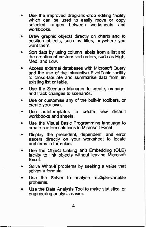
Use the improved drag -and -drop editing facilitywhich can be used to easily move or copyselected ranges between worksheets andworkbooks.

Draw graphic objects directly on charts and toposition objects, such as titles, anywhere youwant them.

Sort data by using column labels from a list andthe creation of custom sort orders, such as High,Med, and Low.

Access external databases with Microsoft Queryand the use of the interactive PivotTable facilityto cross -tabulate and summarise data from anexisting list or table.

Use the Scenario Manager to create, manage,and track changes to scenarios.

Use or customise any of the built-in toolbars, orcreate your own.

to create r ew defaultworkbooks and sheets.

Use the Visual Basic Programming language tocreate custom solutions in Microsoft Excel.

Display the precedent, dependent, and errortracers directly on your worksheet to locateproblems in formulae.

Use the Object Linking and Embedding (OLE)facility to link objects without leaving MicrosoftExcel.

Solve What -if problems by seeking a value thatsolves a formula.

Use the Solver to analyse multiple -variableproblems.

Use the Data Analysis Tool to make statistical orengineering analysis easier.

4

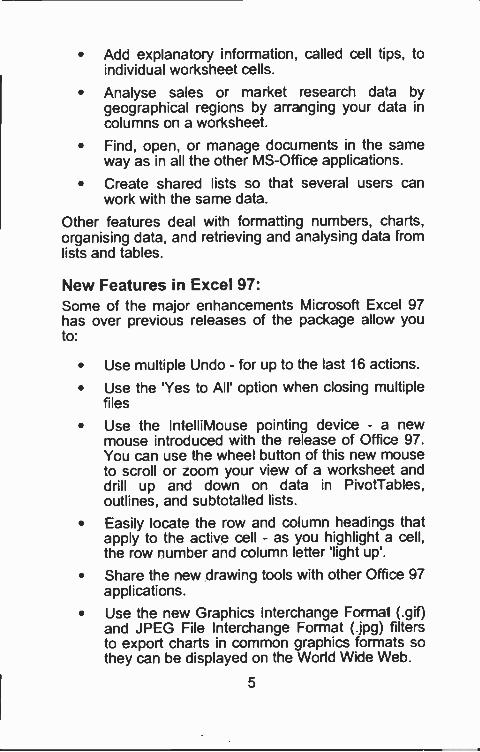
Add explanatory information, called cell tips, toindividual worksheet cells.

Analyse sales or market research data bygeographical regions by arranging your data incolumns on a worksheet.

Find, open, or manage documents in the sameway as in all the other MS -Office applications.

Create shared lists so that several users canwork with the same data.

Other features deal with formatting numbers, charts,organising data, and retrieving and analysing data fromlists and tables.

New Features in Excel 97:Some of the major enhancements Microsoft Excel 97has over previous releases of the package allow youto:

Use multiple Undo - for up to the last 16 actions.

Use the 'Yes to All' option when closing multiplefiles

Use the Inle liMouse pointing device - a newmouse introduced with the release of Office 97.You can use the wheel button of this new mouseto scroll or zoom your view of a workshee-. anddrill up and down on data in PivotTables,outlines, and subtotalled lists.

Easily locate the row and column headings thatapply to the active cell - as you highlight a cell,the row number and column letter 'light up'.

Share the new drawing tools with other Office 97applications.

Use the new Graphics Interchange Formal (.gif)and JPEG F le Interchange Format ( jpg) filtersto export charts in common graphics formats sothey can be displayed on the World Wide Web.

5

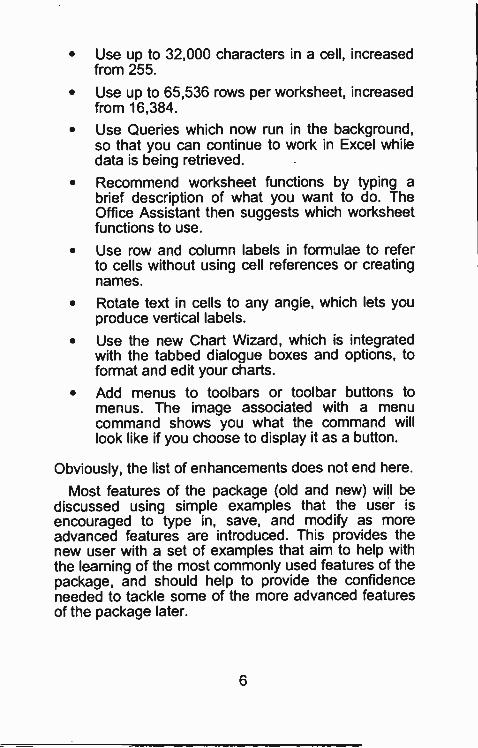
Use up to 32,000 characters in a cell, increasedfrom 255.

Use up to 65,536 rows per worksheet, increasedfrom 16,384.

Use Queries which now run in the background,so that you can continue to work in Excel whiledata is being retrieved.

Recommend worksheet functions by typing abrief description of what you want to do. TheOffice Assistant then suggests which worksheetfunctions to use.

Use row and column labels in formulae to referto cells without using cell references or creatingnames.

Rotate text in cells to any angle, which lets youproduce vertical labels.

Use the new Chart Wizard, which is integratedwith the tabbed dialogue boxes and options, toformat and edit your charts.

Add menus to toolbars or toolbar buttons tomenus. The image associated with a menucommand shows you what the command willlook like if you choose to display it as a button.

Obviously, the list of enhancements does not end here.

Most features of the package (old and new) will bediscussed using simple examples that the user isencouraged to type in, save, and modify as moreadvanced features are introduced. This provides thenew user with a set of examples that aim to help withthe learning of the most commonly used features of thepackage, and should help to provide the confidenceneeded to tackle some of the more advanced featuresof the package later.

6

Installing Excel 97

Installing Excel 97 on your computer's hard disc ismade very easy with the use of the SETUP program,which even configures Excel automatically to takeadvantage of the computer's hardware.

If you are installing from floppy discs, insert the firstSETUP disc (Disc 1) in the A: drive, or if you areinstalling from a CD-ROM, insert the CD in theCD-ROM drive. If you are installing from a networkdrive, make a note of the drive letter because you willneed it later. Then do the following:

Click the Start button on the Windows 95Taskbar and select Settings, Control Panel.

On the displayed Control Panelwindow, double-click the Add/RemovePrograms icon, shown here.

On the Add/Remove Programs Propertiesdialogue box, click the Install/Uninstall tab andpress the Install button.

SETUP will scan your disc for already installedparts of Microsoft Office and will advise you as tothe folder in which you should install Excel. Thiswill most likely be Msoffice.

Follow the SETUP instructions on the sc-een,until the installation of Microsoft Excel programfiles is complete.

The SETUP procram will modify your system filesautomatically and will create a new entry in theStart, Programs cascade menu, with the iconshown here. Clicking this menu entry will startMicrosoft Excel.

If you have MS-Cffice 97 installec, SETUP also addsExcel to the Microsoft Shortcut Bar facility (see nextpage).

7

The Office Shortcut Bar:During installation, the Office Shortcut Bar is collatedand added to the Windows Start Up program so that itwill be displayed automatically on your screenwhenever you start your PC. The contents of aMicrosoft Shortcut Bar used with a previous version ofOffice will be preserved. The Shortcut Bar will bedisplayed when you restart your computer.

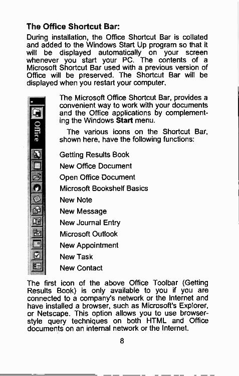
The Microsoft Office Shortcut Bar, provides aconvenient way to work with your documentsand the Office applications by complement-ing the Windows Start menu.

The various icons on the Shortcut Bar,shown here, have the following functions:

Getting Results Book

New Office Document

Open Office Document

Microsoft Bookshelf Basics

New Note

New Message

New Journal Entry

Microsoft Outlook

New Appointment

New Task

New Contact

The first icon of the above Office Toolbar (GettingResults Book) is only available to you if you areconnected to a company's network or the Internet andhave installed a browser, such as Microsoft's Explorer,or Netscape. This option allows you to use browser -style query techniques on both HTML and Officedocuments on an internal network or the Internet.

8

The function of other icons on the toolbar is as follcws:

The New Office Document button: Allows you toselect in the displayed dialogue box the tab conta ningthe type of document you want to work with.Double-clicking the type of document or template youwant, automatically loads the appropriate applicaticn.

The Open Office Document button: Allows ycu towork with an existing document. Opening a document,first starts the application originally used to create i:.

The Microsoft Bookshelf Basics: Allows a preview ofthe world of information found in the complete ve-sionof the Bookshelf which provides access to thee majorreference books; Tne American Heritage Dictionary,The Original Roget's Thesaurus, and The ColumbiaDictionary of Quotations. This facility requires you tohave the CD-ROM.

The New buttons: Allows you to make a New Ncte, aNew Message, or a New Journal Entry to scheduleyour time effectively.

The Microsoft Outlook button: Activates the Office97 new desktop manager used to manage your e-mail,contact lists, tasks and documents.

The New Appointment button: Allows you to add anew appointment in your management system. Thiscaters for all -day or multiple -day events and a meetingplanner, including meeting request processing andattendance lists.The New Task button: Allows you to add a new taskin your management system, including automaticcomposition of an e-mail message summarising a taskand automatic tracking of tasks sent to other users.

The New Contact button: Allows you to enter a newcontact in Outlook's database, or to send an e-mailmessage direct from the contact manager and usehyperlinks for direct access to a contact's home pageon the Internet.

9

The Mouse Pointers

In Microsoft Excel 97, as with all other graphical basedprograms, the use of a mouse makes many operationsboth easier and more fun to carry out.

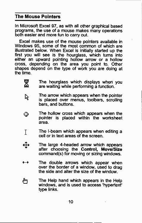
Excel makes use of the mouse pointers available inWindows 95, some of the most common of which areillustrated below. When Excel is initially started up thefirst you will see is the hourglass, which turns intoeither an upward pointing hollow arrow or a hollowcross, depending on the area you point to. Othershapes depend on the type of work you are doing atthe time.

The hourglass which displays when youare waiting while performing a function.

The arrow which appears when the pointeris placed over menus, toolbars, scrollingbars, and buttons.

The hollow cross which appears when thepointer is placed within the worksheetarea.

I The I-beam which appears when editing acell or in text areas of the screen.

4+ The large 4 -headed arrow which appearsafter choosing the Control, Move/Sizecommand(s) for moving or sizing windows.

4-- The double arrows which appear whenover the border of a window, used to dragthe side and alter the size of the window.

The Help hand which appears in the Helpwindows, and is used to access 'hypertext'type links.

10

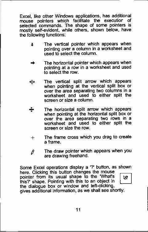
Excel, like other Windows applications, has additionalmouse pointers which facilitate the executior ofselected commands. The shape of some pointers ismostly self-evident, while others, shown below, havethe following functions:

4 The vertical pointer which appears whenpointing over a column n a worksheet andused to select the column.

The ho-izontal pointer which appears whenpointing at a row in a worksheet and usedto select the row.

The vertical split arrow which appearswhen pointing at the vertical split box orover the area separating two columns in aworksheet and used to either split thescreen or size a column.

The horizontal split arrow which appearswhen pointing at the horizontal split box orover ti -e area separating two rows n aworksheet and used to either split thescreen or size the row.

The frame cross which you drag to createa frame.

The draw pointer which appears when youare draw ng freehand.

Some Excel operations display a '?' button, as shownhere. Clicking this Dutton changes :he mousepointer from its usual shape to the 'What'sthis?' shape. Pointing with this to an object inthe dialogue box or window and left -clicking,gives additional information, as we shall see shortly.

11

Using the Office Assistant

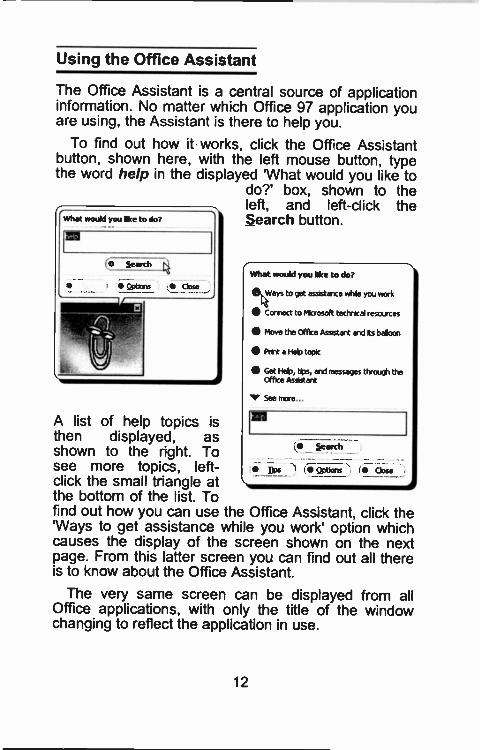
The Office Assistant is a central source of applicationinformation. No matter which Office 97 application youare using, the Assistant is there to help you.

To find out how it works, click the Off ce Assistantbutton, shown here, with the left mouse button, typethe word help in the displayed 'What would you like to

do?' box, shown to theleft, and left -click theSearch button.

what would you like to do?

OC:ays to get assistance while you work.

Connect to Microsoft technical resocrces

Move the Office Assistant and its balloon

Prnt a Help topic

Get Help, tips, and messages through theOffice Assistant

See more..

A list of help topics isthen displayed, as

5earchshown to the right. Tosee more topics, left- . Tips Qptions Closeclick the small triangle atthe bottom of the list. Tofind out how you can use the Office Assistant, click the'Ways to get assistance while you work' option whichcauses the display of the screen shown on the nextpage. From this latter screen you can find out all thereis to know about the Office Assistant.

The very same screen can be displayed from allOffice applications, with only the title of the windowchanging to reflect the application in use.

12

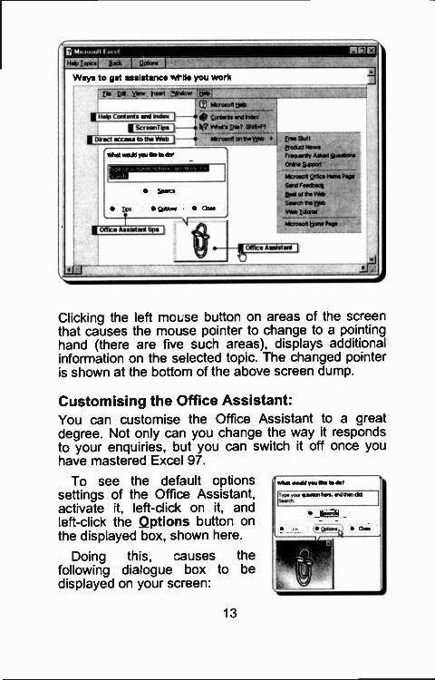
Clicking the left mouse button on areas of the screenthat causes the mouse pointer to change to a pointinghand (there are five such areas), displays additionalinformation on the selected topic. The changed po nteris shown at the bottom of the above screen dump.

Customising the Office Assistant:You can customise the Office Assistant to a creatdegree. Not only can you change the way it -espondsto your enquiries, out you can switch it off once youhave mastered Excel 97.

To see the default optionssettings of the Office Assistant,activate it, left -click on it, andleft -click the Options button onthe displayed box, shown here.

Doing this, causes thefollowing dialogue box to bedisplayed on your screen:

13

Office Assistant

' Assistant c

Respond to FIkey tiove when In the way

Male with wards Guess help topics

1201)1aY alerts P Make founds

Search for both prockrt and proqamming he when wo7amrring

Show bps about

P Using features more effectively r Leyboard shortcuts

P Ltsrq the rnouse more effectively

Other CP oPtuns

r only show NO priority tips

r Show the pp of the Day at startup&eget MY Os

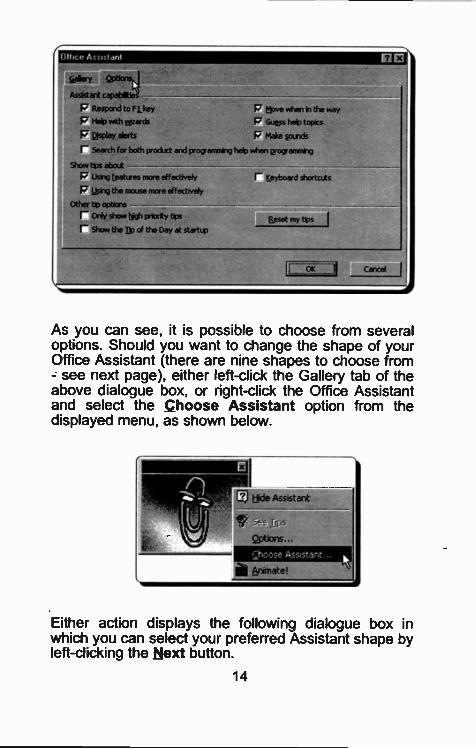
As you can see, it is possible to choose from severaloptions. Should you want to change the shape of yourOffice Assistant (there are nine shapes to choose from- see next page), either left -click the Gallery tab of theabove dialogue box, or right -click the Office Assistantand select the Choose Assistant option from thedisplayed menu, as shown below.

6nimatel

riI

tic:A:stent

.1=1111

Either action displays the following dialogue box inwhich you can select your preferred Assistant shape byleft -clicking the Next button.

14

Office Assistant

StellefY I QptOn

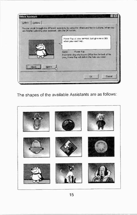
You can scrod through the cifferat assistants by using the <Backend Next> buttons. When yo.,ere finished selecting your assistant dick the OK button.

.,' Power Pup at you serincel Just pure me a :k -kwhen you need help

Norm: Power PupA dynamk dog who mows Office We the back of hepew, Power Pup will delver the help you need.

Reid>

Cancel

The shapes of the available Assistants are as follows:

r

4'

15

Using the Help Menu

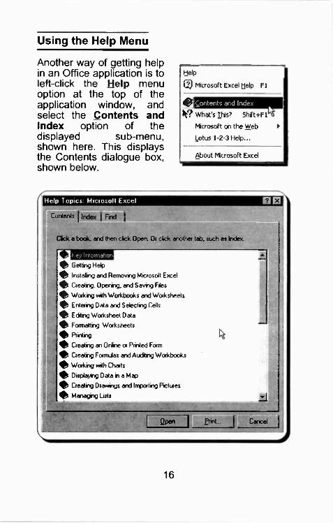
Another way of getting helpin an Office application is toleft -click the Help menuoption at the top of theapplication window, andselect the Contents andIndex option of thedisplayed sub -menu,shown here. This displaysthe Contents dialogue box,shown below.

Help Topics: Microsoft Excel

Contents I Index I Find I

Help

LI Microsoft Excel Help F I

clontents and 'ride.,

le What's This? Shift+F1.1

Microsoft on the Web

Lotus 1-2-3 Help...

About Microsoft Excel

Click a bcck, and then cick Open. Or click another tab, such as Index.

ley Information

* Getting Help Instaling and Removing Microsoft Excel

Creating, Opening, and Saving Files

Working with Workbooks and Worksheets

* Entering Data and Selecting Cells

Editing Worksheet Data Formatting Worksheets

Printing

Deating an Onine or Printed Form

* Creating Formulas and Auciting Workbooks

Working with Charts

Displaying Data in a Map

Dealing Drawings and Importing Pictures

Managing Lists

hS

SIB

2L1

gpen Ernt I Cancel

16

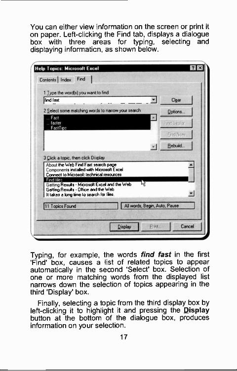
You can either view information on the screen or print iton paper. Left -clicking the Find tab, displays a dialoguebox with three areas for typing, selecting anddisplaying informaticn, as shown below.

( Help Topics: Microsoft Excel

Contents I Index Find I

1 Type the wordfs) you want to find

If Ind last

2 Select some matching wor is to narrow your search

Fa:tfaster

3 click a topic, then click Display

Cliar

Options

Rebuild

About the Web Find Fast search pageComponents installed with ivlicrosoft ExcelConnect to Microsoft techmal resources

Getting Results Microsoft Ex:el and the WebGetting Results Office and the WebIt takes a long time to search Pies

11 Topics Found

.L1

All words, Begin, Auto, Pause

Qisplay Cancel

Typing, for example, the words find fast in the first'Find' box, causes a list of related topics to appearautomatically in the second 'Select' box. Selection ofone or more matching words from the displayed listnarrows down the selection of topics appearing in thethird 'Display' box.

Finally, selecting a topic from the third display box byleft -clicking it to highlight it and pressing the Displaybutton at the bottcm of the dialogue box, producesinformation on your selection.

17

If the topic you want to select is not visible within thedisplay area of the third box, use the scroll bar to get toit.

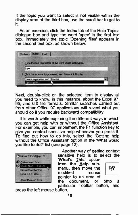
As an exercise, click the Index tab of the Help Topicsdialogue box and type the word 'open' in the first textbox. Immediately the topic 'Opening files' appears inthe second text box, as shown below.

Contents Index I Find I

i, 1 Jype the Int few letters of the word you're looking for.

open

2 ge.k the index entry you want, and then click Display.

online or anizers and lanners

Next, double-click on the selected item to display allyou need to know, in this instance, about the Excel 97,95, and 6.0 file formats. Similar searches carried outfrom other Office 97 applications will reveal what youshould do if you require backward compatibility.

It is worth while exploring the different ways in whichyou can get help with or without the Office Assistant.For example, you can implement the Fl function key togive you context sensitive help whenever you press it.To find out how to do this, select the 'Getting helpwithout the Office Assistant' option in the 'What wouldyou like to do?' list (see page 12).

Another way of getting contextsensitive help is to select the'What's This' optionfrom the Help sub -menu, then move the

I

modified mousepointer to an area ofthe document, or onto aparticular Toolbar button, and

press the left mouse button.

Q Microsoft Excel help Fl

leg Qontents end Index

/1_?11=1111=11111Microsoft on the Web

Lotus 1-2-3 Help...

About Maosoft Excel

18

2. THE EXCEL SPREADSHEET

Starting the Excel Program

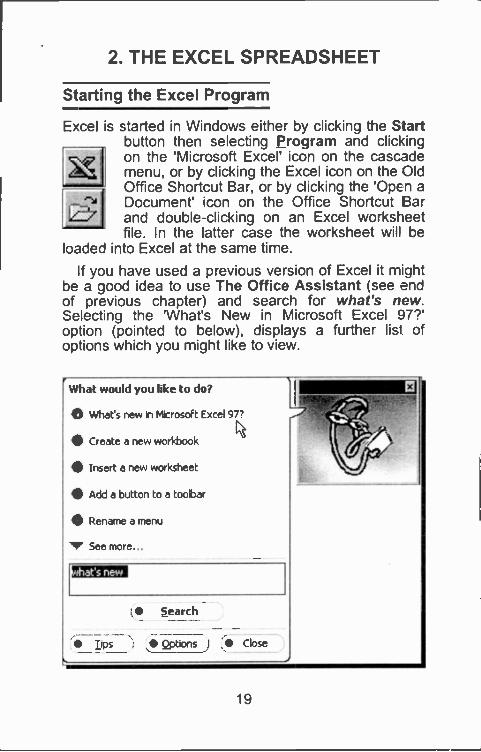
Excel is started in Wiidows either by clicking the Startbutton then selecting Program and clickingon the 'Microsoft Excel' icon on the cascademenu, or by clicking the Excel icon on the OldOffice Shortcut Bar, or by clicking the 'Open aDocument' 'con on the Office Shortcut Barand double-clicking on an Excel worksheetfile. In the latter case the worksheet will be

loaded into Excel at the same time.

If you have used a previous version of Excel it nightbe a good idea to use The Office Assistant (see endof previous chapter') and search for what's new.Selecting the 'What's New in Microsoft Excel 97?'option (pointed to below), displays a further list ofoptions which you might like to view.

What would you like to do?

0 What's new in Microsoft Excel 97?

4 Create a new workbook

Insert a new worksheet

Add a button to a toolba

0 Rename a menu

ir See more...

.

/.4117N:;. '

: ,3-,.

nhat's new

Search

Tips 2ptions Close

19

The Excel Screen

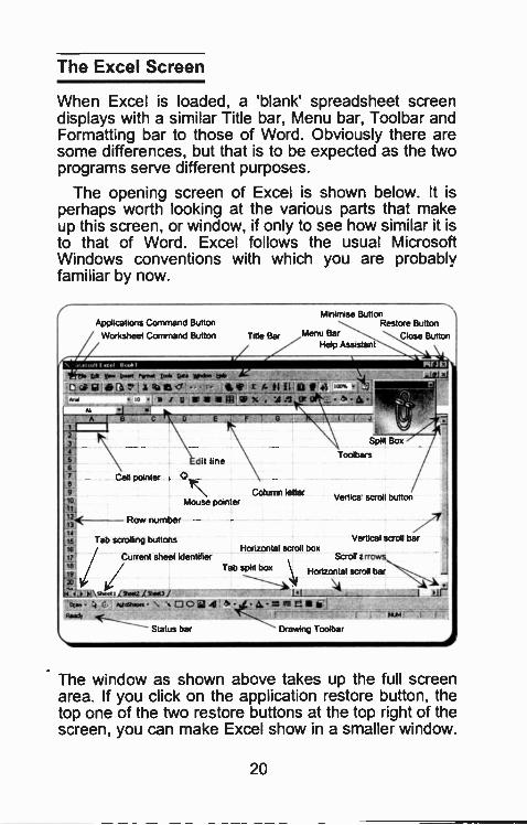
When Excel is loaded, a 'blank' spreadsheet screendisplays with a similar Title bar, Menu bar, Toolbar andFormatting bar to those of Word. Obviously there aresome differences, but that is to be expected as the twoprograms serve different purposes.

The opening screen of Excel is shown below. It isperhaps worth looking at the various parts that makeup this screen, or window, if only to see how similar it isto that of Word. Excel follows the usual MicrosoftWindows conventions with which you are probablyfamiliar by now.

Applications Command Button

Worksheet Command Button Title Bar

Minimise ButtonRestore Button

Menu Bar Close ButtonHelp Assistant

sdie soi. W.. Now two Q.. SM., AeDapioar lears<, sqr ANC Di*/

.0 . B u irwaiRCP/c.:4141 02

it

11;<

is Tab scrolling buttons16

17.. Current sheet identifier'919

Cell pointer

Row number

E F Et

dit line

Column letterMouse pointer

Honzontal scroll box

Split Box

Toolbars

Vertica scroll button

Vertical scroll bar

Scroll E rro

Tab split box Horizontal scr Al bar

.0 p4 siwe I X wag Dhoot3 141

41,61.0. \ ti DJO®4 a. _92 E:

Status bar Drawing Toolbar

The window as shown above takes up the full screenarea. If you click on the application restore button, thetop one of the two restore buttons at the top right of thescreen, you can make Excel show in a smaller window.

20

This can be useful when you are running severalapplications at the same time and ycu want to transferbetween them with the mouse.

Note that the Excel window, which in this casedisplays an empty and untitled book (Book1), hassome areas which rave identical furctions to those ofother Microsoft Office applications, and other areaswhich have different functions. Below, we desc-ibe firstthe areas that are common to other MS -Officeapplications and then :hose that are exclusive to Excel.

Area Function

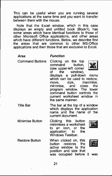
Command Buttons Clicking on the topcommand button,(see upper -left cornerof the window),displays a pull -down menuwhich can be used to restcre,move, size, maximise,minimise, and close :heprogram wirdow. The lowercommand button controls :hecurrent worksheet window inthe same manner.

Title Bar The bar at the top of a windowwhich displays the applicationname and the name of :hecurrent document.

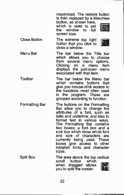
Minimise Button Clicking this buttonminimises a worksheetto an icon, or theapplication to theWindows Taskbar.

Restore Button When clicked on, thisbutton restores theactive window to theposition and size thatwas occupied before it was

21

Close Button

Menu Bar

Toolbar

Formatting Bar

Split Box

maximised. The restore buttonis then replaced by a Maximisebutton, as showr here,which is used setthe window to fullscreen size.

The extreme top rightbutton that you click toclose a window.

The bar below the Title barwhich allows you to choosefrom several menu options.Clicking on a menu itemdisplays the pu I -down menuassociated with that item.

The bar below the Menu barwhich contains buttons thatgive you mouse -click access tothe functions mcst often usedin the program. These aregrouped according to function.

The buttons on the FormattingBar allow you to change theattributes of a font, such asitalic and underline, and also toformat text in various ways.The Formatting Bar containstwo boxes; a font box and asize box which show which fontand size of characters arecurrently being used. Theseboxes give access to otherinstalled fonts and charactersizes.

The area above the top verticalscroll button whichwhen dragged allowsyou to split the screen.

22

-+-

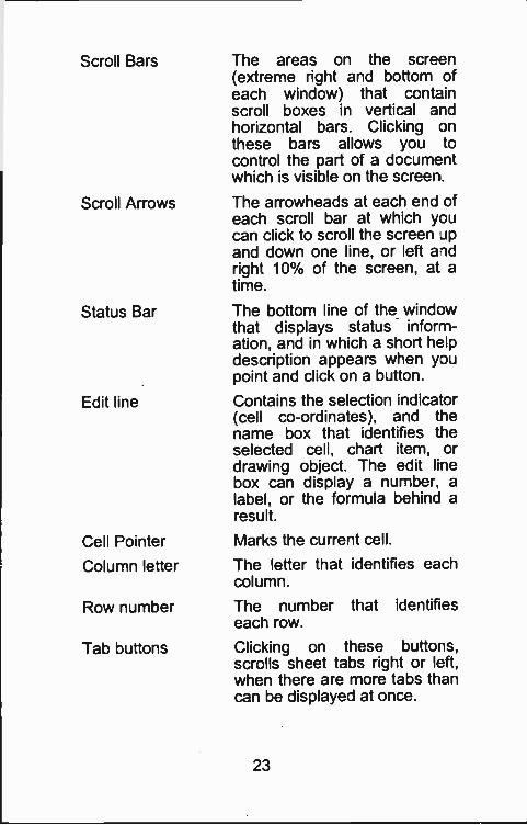
Scroll Bars

Scroll Arrows

Status Bar

Edit line

Cell Pointer

Column letter

Row number

Tab buttons

The areas on the screen(extreme right and bottom ofeach window) that containscroll boxes in vertical andhorizontal bars. Clicking onthese bars allows you tocontrol the part of a documentwhich is visible on the screen.

The arrowheads at each end ofeach scroll bar at which youcan click to scroll the screen Jpand down one line, or left andright 10% of the screen, at atime.

The bottom line of the windowthat displays status inform-ation, and in which a short helpdescription appears when youpoint and click on a button.

Contains the selection indica:or(cell co-ordinates), and thename box that identif es theselected cell, chart item, ordrawing object. The edit linebox can display a number, alabel, or the formula behind aresult.

Marks the current cell.

The letter that identifies eachcolumn.

The number that identifeseach row.

Clicking on these buttons,scrolls sheet tabs right or left,when there are more tabs thancan be displayed at once.

23

Current sheet

Tab split box

Shows the current sheet amongsta number of sheets in a file. Theseare named Sheetl , Sheet2,Sheet3, and so on, by default, butcan be changed to, say, North,South, East, and West. Clicking ona sheet tab, moves you to thatsheet.

The split box which you drag left tosee more of the scroll bar, or rightto see more tabs.

Excel 97 has two split boxes, which are used to splitthe screen horizontally or vertically. One of these islocated at the extreme right of the screen above the'top vertical scroll arrow' button, and is identified onExcel's worksheet screen dump showr on page 20.The other is located at the extreme bottom -right cornerof the screen, to the left of the 'right horizontal scrollarrow' button, but is not identified on our screen dump.Both of these have to do with splitting the screen; theidentified one horizontally, the other vertically. The useof both these split boxes will be discussed later.

The Menu Bar Options:Each menu bar option has associated with it apull -down sub -menu. To activate the menu, eitherpress the <Alt> key, which causes the first option of themenu (in this case the current Book Control Menu box)to be highlighted, then use the right and eft arrow keysto highlight any of the options in the menu, or use themouse to point to an option. Pressing either the<Enter> key, or the left mouse button, reveals thepull -down sub -menu of the highlighted menu option.

24

X Microsoft Excel - Sqdb.xls

Fderx

Ctrl+N

Open... Ctr1+0

Close

61 Save Ctrl+S

Save .

Save as dTML...

Save Workspace...

Page Setup...

Print Area

aPrint Preview

a Dint- Ctr1-1-P

Send To

Properties

iSqdb.xls

Podb.xls

2 Invdb.xls

4 Expdb.xls

Exit

time, closes the

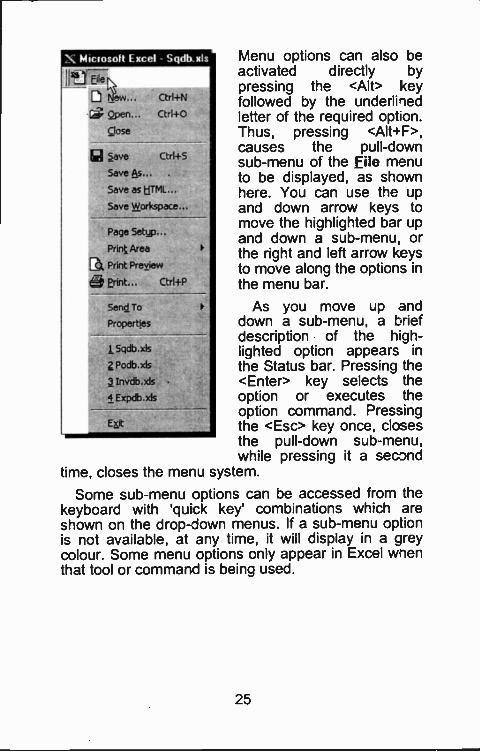
Menu options can also beactivated directly bypressing the <Alt> keyfollowed by the underliiedletter of the required opt on.Thus, pressing <Alt+F>,causes the pull -downsub-ment.. of the File menuto be displayed, as shownhere. You can use the upand down arrow keys tomove the highlighted bar upand down a sub -menu, orthe right and left arrow keysto move along the options inthe menu bar.

As you move up anddown a sub -menu, a briefdescription of the h gh-lighted option appears inthe Status bar. Pressing the<Enter> key selects theoption or executes theoption ccmmand. Pressingthe <Esc> key once, closesthe pull -down sub -menu,while pressing it a second

menu system.

Some sub -menu options can be accessed from thekeyboard with 'quick key' combinations which areshown on the drop -down menus. If a sub-mer u optionis not available, at any time, it will display in a areycolour. Some menu cptions only appear in Excel wrenthat tool or command is being used.

25

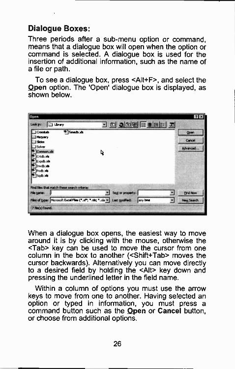
Dialogue Boxes:Three periods after a sub -menu option or command,means that a dialogue box will open when the option orcommand is selected. A dialogue box is used for theinsertion of additional information, such as the name ofa file or path.

To see a dialogue box, press <Alt+F>, and select theQpen option. The 'Open' dialogue box is displayed, asshown below.

Open

ook r: I _j Lbr cry *1(73131 itlEf I _MICrosstab

--I Mums,'"-J Sides,--150iverjCanmon.zisiCrtdb.

xpcb.xls

Irrocto. xis

+jpom.xb_15qcb. xis

4,ibrnedb. xis

Cancel I

fylveceed... I

Rnd ties that match these sesch crtericFie Done: II Ted or property: I Einciar.

Fees of type: IMKroseft Excel Hes (. or; .xls list lorry trre

7 fie(s) found.

When a dialogue box opens, the easiest way to movearound it is by clicking with the mouse, otherwise the<Tab> key can be used to move the cursor from onecolumn in the box to another (<Shift+Tao> moves thecursor backwards). Alternatively you can move directlyto a desired field by holding the <Alt> key down andpressing the underlined letter in the field name.

Within a column of options you must use the arrowkeys to move from one to another. Having selected anoption or typed in information, you must press acommand button such as the Qpen or Cancel button,or choose from additional options.

26

To select the Open button with the mouse, simply pointand click, while with the keyboard you must first p-essthe <Tab> key until the dotted rectangle moves to therequired button, and then press the <Enter> -ey.Pressing <Enter> at any time while a dialogue bcx isopen, will cause the marked items to be selected andthe box to be closed.

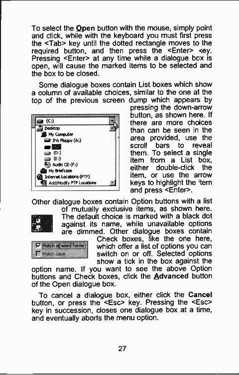
Some dialogue boxes contain List boxes which snowa column of available choices, similar to the one at thetop of the previous screen dump which appears by

pressing the down-arrowbutton, as shows here. Ifthere are more choicesthan can be seen in thearea provided, use thescroll bars to revealthem. To select a siigleitem from a List Dox,either double-click theitem, or use the arrowkeys to highlight the ternand press <Enter>.

Other dialogue boxes contain Option buttons with a listof mutually exclusive items, as shown here.The default choice is marked with a Dlack dotagainst its name, while unavailable opt:onsare dimmed. Other dialogue boxes contain

Check boxes, like the one here,which offer a list of options you canswitch on or off. Selected optionsshow a tick in the box against the

option name. If you want to see the above Optionbuttons and Check boxes, click the Advanced buttonof the Open dialogue box.

To cancel a dialogue box, either click the Cancelbutton, or press the <Esc> key. Pressing the <Esc>key in succession, closes one dialogue box at a t me,and eventually aborts the menu option.

(C:) _kt

- Desktop

A My Computer31/2 Floppy (4:) a(D)(E :)

4;) Audio CD (F:)My Briefcase

Internet Locations (FTP)

Acid/Modify FTP locations .:J

a AndC or

r Ni 4c, case

27

Workbook Navigation

When you first enter Excel, the program sets up aseries of huge electronic pages, or worksheets, in yourcomputer's memory, many times larger than the smallpart shown on the screen. Individual cells are identifiedby column and row location (in that order), with presentsize extending to 256 columns and 65,536 rows. Thecolumns are labelled from A to Z, followed by AA to AZ,BA to BZ, and so on, to IV, while he rows arenumbered from 1 to 65,536.

A worksheet can be thought of as a two-dimensionaltable made up of rows and columns. The point where arow and column intersect is called a cell, while thereference points of a cell are known as the celladdress. The active cell (Al when you first enter theprogram) is boxed. A workbook is made up of differentworksheets stacked 'on top of each other'.

Navigation around a worksheet is achieved by usingone of the following keys or key combinations:

Pressing one of the four arrow keys (-44-1')moves the active cell one position right, down,left or up, respectively.

Pressing the <PgDn> or <PgUp> keys movesthe active cell down or up one visible page.

Pressing the <Ctrl+-*> or <Ctrl+1> keycombinations moves the active cell to theextreme right of the worksheet (column IV) orextreme bottom of the worksheet (row 65,536).

Pressing the <Home> key, moves the active cellto the beginning of a row.

Pressing the <Ctrl+Home> key combinationmoves the active cell to the home position, Al.

Pressing the <Ctrl+End> key combination movesthe active cell to the lower right corner of theworksheet's currently used area.

28

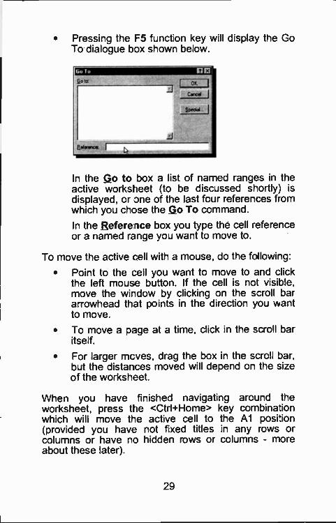
Pressing the F5 function key will display the GoTo dialogue box shown below.

Go To

go ta

asionowo

OK

Lst

In the Go to box a list of named ranges in theactive worksheet (to be discussed st-ortly; isdisplayed, or one of the last four references fromwhich you chose the Go To ccmmand.

In the Reference box you type the cell referenceor a named range you want to move to.

To move the active cell with a mouse, do the following:

Point to the cell you want to move to and clickthe left mouse button. If the cell is no: visible,move the window by clicking on the scroll bararrowhead that points in the direction you wantto move.

To move a pace at a time, click in the scroll baritself.

For larger mcves, drag the bcx in the scroll bar,but the distances moved will cepend on the sizeof the worksheet.

When you have finished navigating around theworksheet, press the <Ctrl+Home> key combinationwhich will move the active cell to the Al position(provided you have not fixed titles in any rows orcolumns or have no hidden rows cr columns - moreabout these later).

29

Note that the area within which you can move theactive cell is referred to as the working area of theworksheet, while the letters and numbers in the borderat the top and left of the working area give the'co-ordinates' of the cells in a worksheet.

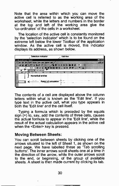
The location of the active cell is constantly monitoredby the 'selection indicator' which is to be found on theextreme left below the lower Toolbar of the applicationwindow. As the active cell is moved, this indicatordisplays its address, as shown below.

Selection indicator Edit line

t9 o. got v.. rwt r zoo, co. tem.. wefil m7! gel A eta

.,0 elrirx gear.M.A2A3A18,C0

6Numerical entries

Result of calculation

a

The contents of a cell are displayed above the columnletters within what is known as the 'Edit line'. If youtype text in the active cell, what you type appears inboth the 'Edit line' and the cell itself.

Typing a formula which is preceded by the equalssign (=) to, say, add the contents of three cells, causesthe actual formula to appear in the 'Edit line', while theresult of the actual calculation appears in the active cellwhen the <Enter> key is pressed.

Moving Between Sheets:You can scroll between sheets by clicking one of thearrows situated to the left of Sheet 1, as shown on thenext page. We have labelled these as 'Tab scrollingbuttons'. The inner arrows scroll sheets one at a time inthe direction of the arrow, while the outer arrows scrollto the end, or beginning, of the group of availablesheets. A sheet is then made current by clicking its tab.

30

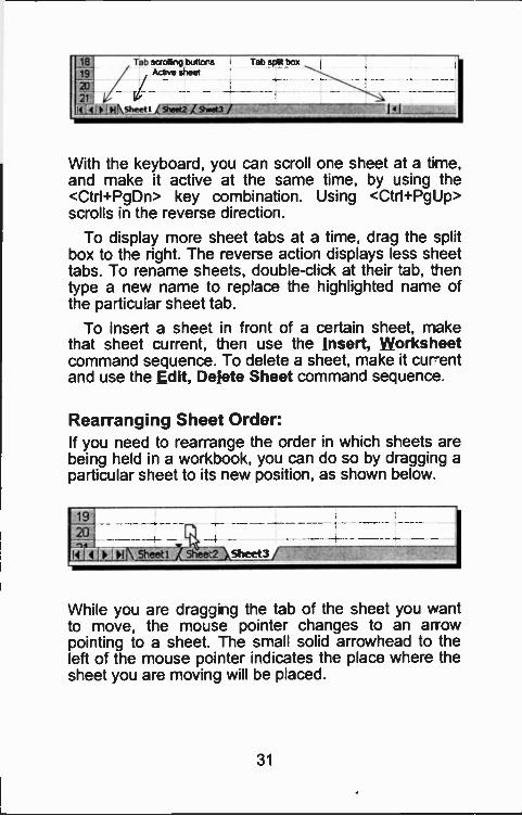
18_119!

2t4:41,41Mheetlijkiet2LRvItitli

Tab scrolling buttors Tab split boxActive sheet

With the keyboard, you can scroll one sheet at a time,and make it active at the same time, by using the<Ctrl+PgDn> key combination. Using <Ctri+PgUp>scrolls in the reverse direction.

To display more sheet tabs at a time, drag the splitbox to the right. The reverse action displays less sheettabs. To rename sleets, double-click at their tab, thentype a new name to replace the highlighted name ofthe particular sheet tab.

To insert a shee: in front of a certain sheet, makethat sheet current, then use the Insert, Worksheetcommand sequence. To delete a sheet, make it curentand use the Edit, Delete Sheet command sequence.

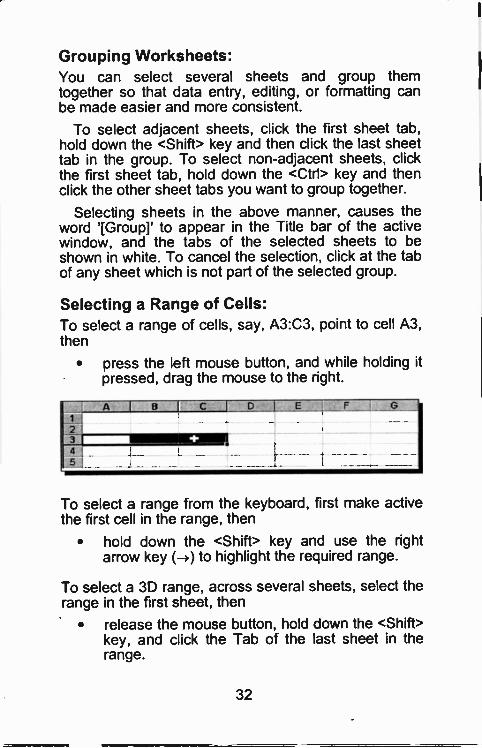
Rearranging Sheet Order:If you need to rearrange the order in which sleets arebeing held in a workbook, you can do so by dragging aparticular sheet to its new position, as shown below.

19

20

W1V5hee____5heec heet3/

While you are dragging the tab of the sheet you wantto move, the mouse pointer changes to an arrowpointing to a sheet. The small solid arrowhead to theleft of the mouse pointer indicates the place where thesheet you are moving will be placed.

31

Grouping Worksheets:You can select several sheets and group themtogether so that data entry, editing, or formatting canbe made easier and more consistent.

To select adjacent sheets, click the fist sheet tab,hold down the <Shift> key and then click the last sheettab in the group. To select non -adjacent sheets, clickthe first sheet tab, hold down the <Ctrl> key and thenclick the other sheet tabs you want to group together.

Selecting sheets in the above manner, causes theword '[Group]' to appear in the Title bar of the activewindow, and the tabs of the selected sheets to beshown in white. To cancel the selection, click at the tabof any sheet which is not part of the selected group.

Selecting a Range of Cells:To select a range of cells, say, A3:C3, point to cell A3,then

press the left mouse button, and while holding itpressed, drag the mouse to the right.

AIBICI4

5

To select a range from the keyboard, first make activethe first cell in the range, then

hold down the <Shift> key and use the rightarrow key (-3) to highlight the required range.

To select a 3D range, across several sheets, select therange in the first sheet, then

release the mouse button, hold down the <Shift>key, and click the Tab of the last sheet in therange.

32

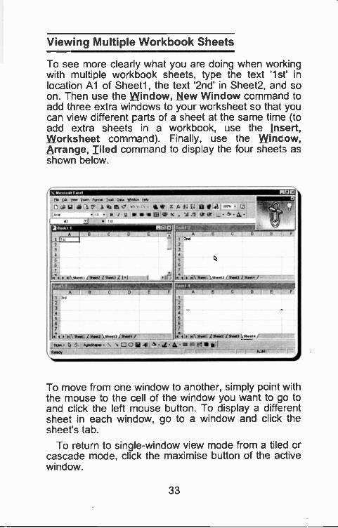
Viewing Multiple Workbook Sheets

To see more clearly what you are doing when workingwith multiple workbook sheets, type the text '1st' inlocation Al of Sheetl, the text '2nd in Sheet2, and soon. Then use the Window, New Window command toadd three extra windows to your wo-ksheet so that youcan view different parts of a sheet at the same time (toadd extra sheets in a workbook, use the Insert,Worksheet command). Finally, use the Wincow,Arrange, Tiled command to display the four sheets asshown below.

Cr GA

DEG (.4 V'

-111st

ed.. 1*pa a cf . fr r A flit

it 1 g vonitlePx.'Ael OE* _&8.

Pinn.

12111

6

11.14 IA *mei ),sn...tz ifitrO3 Rest4

3

A

\7..i X 9..2 ).....43

A

3

5

6

N.1 I M Ihmtl 4.2 *AAP

Ct. 4 A.RAS.c. \ DO El, g A, u,7. --e 6ANS

To move from one w ndow to another, simply point withthe mouse to the cell of the window you want to co toand click the left mcuse button. To display a differentsheet in each window, go to a window and click thesheet's tab.

To return to single -window view mode from a tiled orcascade mode, click the maximise button of the activewindow.

33

Entering Information

We will now investigate how information can beentered into a worksheet. But first, make sure you arein Sheeti , then return to the Home (Al position, bypressing the <Ctrl+Home> key combination, then typethe words:

PROJECT ANALYSIS

As you type, the characters appear in both the 'Editline' and the active cell. If you make a mistake, pressthe <BkSp> key to erase the previous letter or the<Esc> key to start again. When you have finished,press <Enter>.

Note that what you have just typed in has beenentered in cell A1, even though the whole of the wordANALYSIS appears to be in cell B1. If you use the rightarrow key to move the active cell to B1 you will seethat the cell is indeed empty.

Typing any letter at the beginning of an entry into acell results in a 'text' entry being formed automatically,otherwise known as a 'label'. If the length of the text islonger than the width of a cell, it will continue into thenext cell to the right of the current active cell, providedthat cell is empty, otherwise the displayed informationwill be truncated.

To edit information already in a cell, either

double-click the cell in question, or

make that cell the active cell and press the F2function key.

The cursor keys, the <Home> and <End> keys, as wellas the <Ins> and <Del> keys can be usec to move thecursor and/or edit information as required.

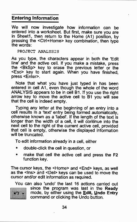
You can also 'undo' the last 16 actions carried outsince the program was last in the Readymode, by either using the Edit, undo Entrycommand or clicking the Undo button.

34

Next, move the active cell to B3 and typeJan

Pressing the right arrow key (-) will automaticallyenter the typed information into the cell and also movethe active cell one cell to the right, in this case to C3.Now type

Feb

and press <Enter>.

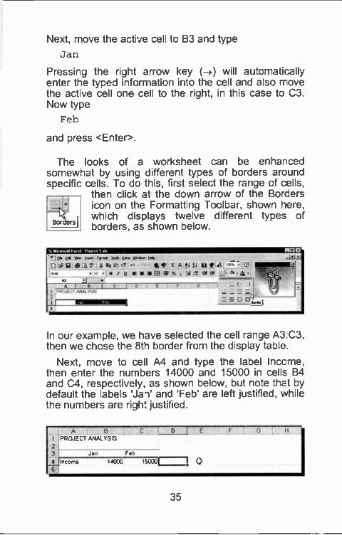
The looks of a worksheet can be enharcedsomewhat by using different types of borders arcundspecific cells. To do This, first select the range of cells,

then click at the down arrow of the Bordersicon on ttse Formatting Toolbar, shown here,which displays twelve different types ofborders, as shown below.

I .r rl 14,1-1 I Eh

cat Dd. too

61 II Jl t4 iJ 4i/11SEMW)14.14Afarbr _1-&/

IHe r C C

ANAL

Fe 0 1:1

An©

In our example, we have selected the cell range A3:C3,then we chose the 8t'l border from the display table.

Next, move to cell A4 and type the label Income,then enter the numbers 14000 and 15000 in cells B4and C4, respectively, as shown below, but note that bydefault the labels 'Jag' and 'Feb' are left justified, whilethe numbers are righ: justified.

A1 PROJECT ANALYSIS2

3 Jan Feb

Income 14000 15020 I 05

35

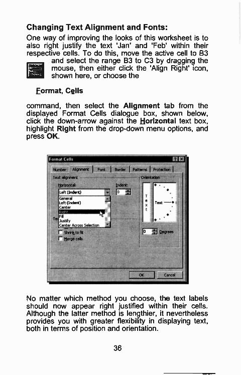
Changing Text Alignment and Fonts:One way of improving the looks of this worksheet is toalso right justify the text 'Jan' and 'Feb' within theirrespective cells. To do this, move the active cell to B3

and select the range B3 to C3 by dragging themouse, then either click the 'Align Right' icon,shown here, or choose the

Format, Cells

command, then select the Alignment tab from thedisplayed Format Cells dialogue box, shown below,click the down-arrow against the Horizontal text box,highlight Right from the drop -down menu options, andpress OK.

No matter which method you choose, the text labelsshould now appear right justified within their cells.Although the latter method is lengthier, it neverthelessprovides you with greater flexibility in displaying text,both in terms of position and orientation.

36

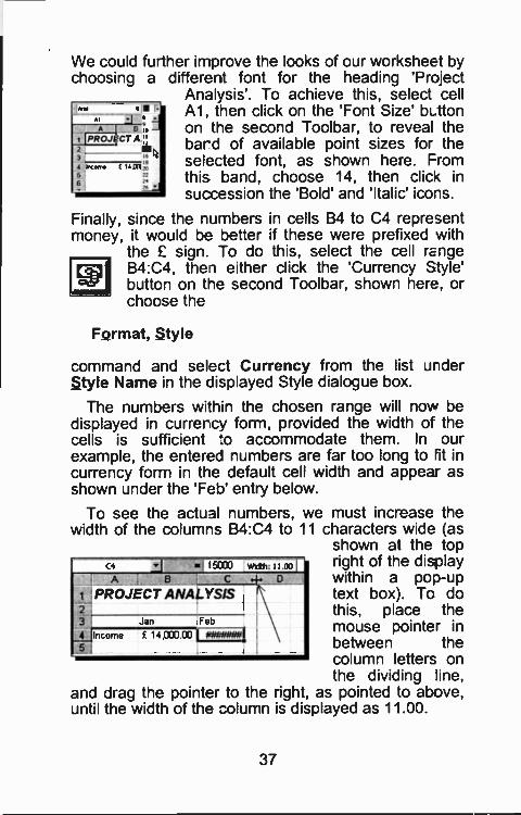
We could further imp-ove the looks of our worksheet bychoosing a different font for the heading 'Project

Analysis'. To achieve this, select cellA1, then click on the 'Font Size' buttonon the second Toolbar, to reveal thebard of available point sizes for theselected font, as shown here. Fromthis band, choose 14, then click insuccession the 'Bold' and 'Italic' icons.

Finally, since the numbers in cells B4 to C4 representmoney, it would be better if these were prefixed with

the £ sign. To do this, se.ect the cell re ngeB4:C4, thei either click the 'Currency Style'button on the second Toolbar, shown here, orchoose the

Ansi

Ai

A

I IPROJE2

3

- -le^ d

Lc

CT A.::1111

4 In, or,66

14 al

FQrmat, Style

command and select Currency from the list underStyle Name in the displayed Style d alogue box.

The numbers within the chosen range will now bedisplayed in currercy form, provided the width of thecells is sufficient -.0 accommodate them. In ourexample, the entered numbers are far too long to 1t incurrency form in tl-e default cell width and appear asshown under the 'Feb' entry below.

To see the actual numbers, we must increase thewidth of the columns B4:C4 to 11 characters wide (as

shown at the topC4 150013 vedtti: It 00 right of the displayA B c o within a pop-up

PROJECT ANALYSIS text box). To do2

Jan Febthis, place themouse pointer in

AlIncome £ 14,000031 $40,###$ .

5_ I between thecolumn letters onthe dividing line,

and drag the pointer to the right, as pointed to above,until the width of the column is displayed as 11.00.

37

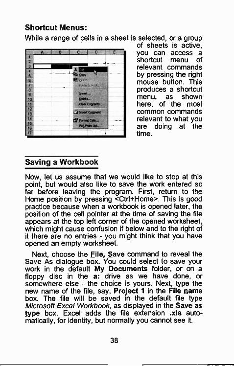
Shortcut Menus:While a range of cells in a sheet

a

2

34 X MEI.

litti Lan

a9

_113

122

13.14161

16

17

Valets...

Coptents

Li inset coopent

Eonbet

Pkt From Ust...

Saving a Workbook

is selected, or a groupof sheets is active,you can access ashortcut menu ofrelevant commandsby pressing the rightmouse button. Thisproduces a shortcutmenu, as shownhere, of the mostcommon commandsrelevant to what youare doing at thetime.

Now, let us assume that we would like to stop at thispoint, but would also like to save the work entered sofar before leaving the program. First, return to theHome position by pressing <Ctrl+Home>. This is goodpractice because when a workbook is opened later, theposition of the cell pointer at the time of saving the fileappears at the top left corner of the opened worksheet,which might cause confusion if below and :o the right ofit there are no entries - you might think that you haveopened an empty worksheet.

Next, choose the File, Save command to reveal theSave As dialogue box. You could select to save yourwork in the default My Documents folder, or on afloppy disc in the a: drive as we have done, orsomewhere else - the choice is yours. Next, type thenew name of the file, say, Project 1 in the File namebox. The file will be saved in the default file typeMicrosoft Excel Workbook, as displayed in the Save astype box. Excel adds the file extension .xls auto-matically, for identity, but normally you cannot see it.

38

Save As 17E3

Sive r I -.., A :1 _LI L --11711.193J

ZEMKE

. .:

Carol

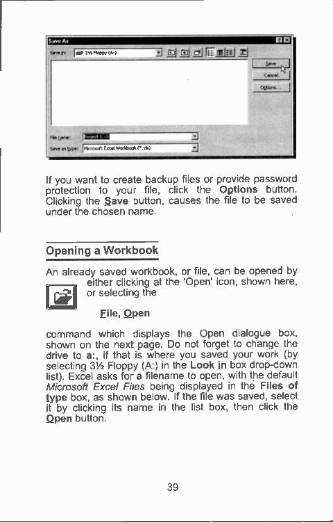
If you want to create backup files or provide passwordprotection to you- file, click the Options button.Clicking the Save Dutton, causes the file to be savedunder the chosen name.

Opening a Workbook

An already saved workbook, or file, can be opened byeither clicking at the 'Open' icon, shown here,or selecting the

File, Qpen

command which displays the Open dialogue box,shown on the next page. Do not forget to change thedrive to a:, if that is where you saved your work (byselecting 31/2 Floppy (A:) in the Look in box drop -downlist). Excel asks for a filename to open, with the defaultMicrosoft Excel Files being displayed in the Files oftype box, as shown below. If the file was saved, selectit by clicking its name in the list box, then click theQpen button.

39

Open

Look iri: I.e7 31/2 Flcopy ('a:)

IsiProSect 1.xis

:21(11551 iFz rolEtlEil 2_13

El©

Qp.

Cancel

'advanced-.

Fax/ Has that match thew search Mena.

flame: II L'Fie End NowZ.1 19.1 or Prilcadll

Flies at Voir: Ilicroscit Excel Fies e, xis, stszi Last wells& Ianytime 11 Nett Search

Na(s)Card.

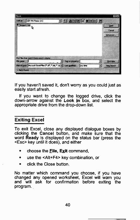
If you haven't saved it, don't worry as you could just aseasily start afresh.

If you want to change the logged drive, click thedown-arrow against the Look in box, and select theappropriate drive from the drop -down list.

Exiting Excel

To exit Excel, close any displayed dialogue boxes byclicking the Cancel button, and make sure that theword Ready is displayed on the status bar (press the<Esc> key until it does), and either

choose the File, Exit command,

use the <Alt+F4> key combination, or

click the Close button.

No matter which command you choose, if you havechanged any opened worksheet, Excel will warn youand will ask for confirmation before exiting theprogram.

40

3. FILLING IN A WORKSHEET

We will use, as ar example on how a worksheet canbe built up, the few entries on 'Project Analysis' from

the previous chapter. If you have savedProject 1, then either click the Open button,or use the Eile, Open command, thenhighlight its filename in the Open dialogue

box, and click the OK button. If you haven't saved it,don't worry as you could just as easily start afresh.

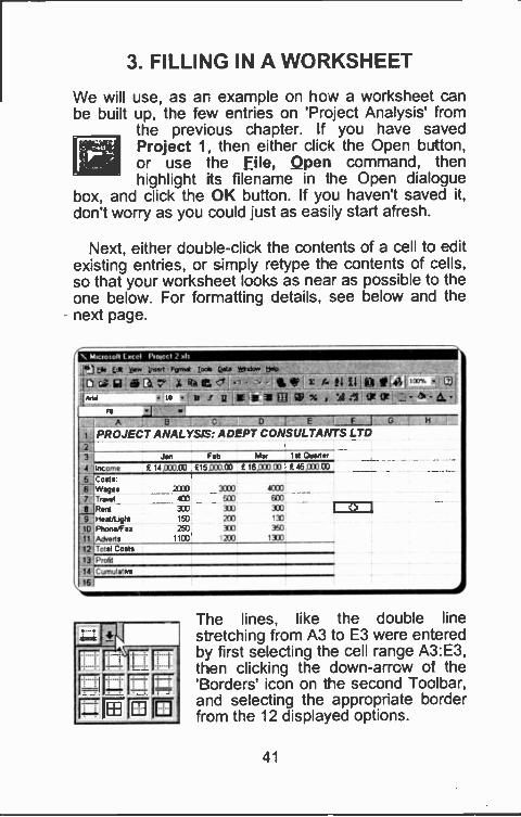
Next, either double-click the contents of a cell to editexisting entries, or simply retype the contents of cells,so that your worksheet looks as near as possible to theone below. For formatting details, see below and thenext page.

\ elictotott [met Poteect 2 x11

_en Ek La i'... in.rt Ftrme tom. L.*. 10,do. !PO

ID a la o a z.. x 16 e <-, - 11 ft x f- t 1 li CS II 41 ' - - 91,..., , a r IIE a N EH Wx , V ;I OF Or _ - a' d-

8 I]A e 0 D E F I G H

PROJECT ANALYSIS: ADEPT CONSULTANTS LTD2

3

4

Jan Ireb Mal 1st Quarter

Income £ 14,0:0 CO £15130000 f 16,!033 £ 45.1333.00

Azle

Coat,Wages 2033 3000 4030

Travel 403 503 033

iz, Rent 333 300 330 1

,9..Heal/Light 1W 200 133A Phona/Fax 250 311 350

'1415Adhuts 1103 '200 1330

1ZTotal CosttneProil

1.1 Cuntutatret

177

11-7FE [MD

The lines, like the double linestretching from A3 to E3 were enteredby first selecting the cell range A3:E3,then clicking the down-arrow of the'Borders' icon on the second Toolbar,and selecting the appropriate borderfrom the 12 displayed options.

41

Formatting Entries

The information in cell Al (PROJECT ANALYSIS:ADEPT CONSULTANTS LTD) was entered left justifiedand formatted by clicking on the 'Font Size' button onthe Formatting Toolbar, and selecting 14 point font size

from the band of available font sizes, thenclicking in succession the 'Bold' and 'Italic'icons.

The text in the cell block B3:E3 was formatted by firstselecting the range and then clicking the 'Centre'

alignment icon on the second Toolbar, so thetext within the range was displayed centrejustified.

The numbers within the cell block B4:E4 wereformatted by first selecting the range, then clicking the'Currency Style' icon on the second Toolbar, shown

here, so the numbers appeared with two digitsafter the decimal point and prefixed with the £sign.

All the text appearing in column A (apart from that incell Al) was just typed in (left justified), as shown in thescreen dump on the previous page.

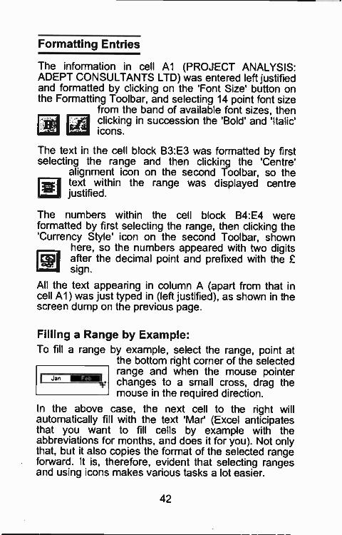
Filling a Range by Example:To fill a range by example, select the range, point at

the bottom right corner of the selectedrange and when the mouse pointer

I Jan1111122.0 changes to a small cross, drag the

mouse in the required direction.

In the above case, the next cell to the right willautomatically fill with the text 'Mar' (Excel anticipatesthat you want to fill cells by example with theabbreviations for months, and does it for you). Not onlythat, but it also copies the format of the selected rangeforward. It is, therefore, evident that selecting rangesand using icons makes various tasks a lot easier.

42

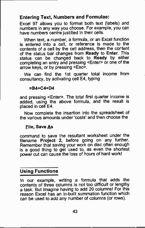
Entering Text, Numbers and Formulae:Excel 97 allows you to format boti text (labels) andnumbers in any way you choose. For example, you canhave numbers cent -e justified in their cells.

When text, a number, a formula, or an Excel functionis entered into a cell, or reference is made to thecontents of a cell by the cell address, then the cortentof the status bar changes from Ready to Enter. Thisstatus can be charged back to Ready by eithercompleting an entry and pressing <Enter> or one cor thearrow keys, or by p-essing <Esc>.

We can find the 1st quarter total income fromconsultancy, by activating cell E4, typing

=B4+C4+D4

and pressing <Enter>. The total first quarter income isadded, using the above formula, and the result isplaced in cell E4.

Now complete the insertion into the spreadsheet ofthe various amounts under 'costs' and then choose the

File, Save As

command to save tie resultant worksheet under thefilename Project 2, before going on any furter.Remember that saving your work on disc often enoughis a good thing to get used to, as even the shortestpower cut can cause the loss of hours of hard work!

Using Functions

In our example, writing a formula that adds thecontents of three columns is not too difficult or lergthya task. But imagine having to add 20 columns! For thisreason Excel has ar in-built summation function whichcan be used to add any number of columns (or rows).

43

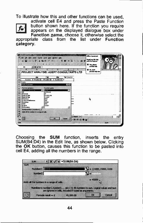
To illustrate how this and other functions can be used,activate cell E4 and press the Paste Functionbutton shown here. If the function you requireappears on the displayed dialogue box underFunction name, choose it, otherwise select the

appropriate class from the list under Functioncategory.

f

La. N.. 1.4 8...1 1lf 1116Gil 7 s. Re r.

X J

ar) .

A 11 G L) E I r

PROJECT ANALYSIS: ADEPT CONSULTANTS LTD

I'VdrCIVDale If lwe ow9,14M4%. C.AINT

In.. a Rd., ort14 IAaasse

Is16

17 strsfravnber Aurrate42,,_)IS Mil, al am rosnbwt r .1.19

I«

I I

Edn

greAtle help

4.44. 1.1

44. irNUM

Choosing the SUM function, inserts the entrySUM(B4:D4) in the Edit line, as shown below. Clickingthe OK button, causes this function to be pasted intocell E4, adding all the numbers in the range.

SUM X J1=i =SUM(B4:D4)

Plumber' 11111/ 04030,15000,16001Nurnber21

Adds d the numbers h a range of cells.45000

flurnber 1: number I,nurnber2,... are 1 to 30 rurbers to sun. Logical values end textare Ignored h oak, Included I typed as arganents.

ED Formula f 45,000.00 OK Cancel

44

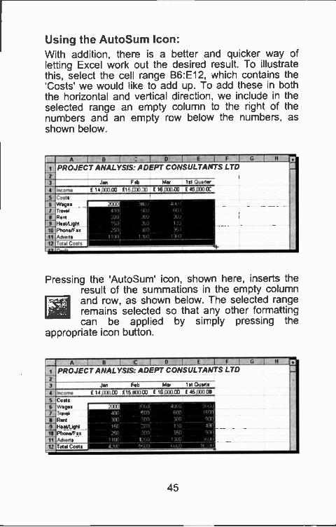
Using the AutoSum Icon:With addition, there is a better and quicker way ofletting Excel work out the desired result. To illustratethis, select the cell range B6:E12, which contains the'Costs' we would like to add up. To add these in boththe horizontal and vertical direction, we include in theselected range an empty column to the right of thenumbers and an empty row below the numbers, asshown below.

III=131111111171111111111111M111111MEINIIIM111111 IINIMINICIIIIIMCB11 aINi

IAEl

(Income

Qnliglimri0in

PROJECT ANALYSIS. ADEPT CONSULTANTS LTD

Jan Fib Mar 1st Quarter

(1400000 f15 110 f16ttt 00 f 45 1 CC

CostsWages .III]TravelRent .,JJ Aw .4,.tleatillght 1501 .10 13J

Phoneff as 2501 ice Yr,Adverts I trill I AO I9"0

12 Total CostsMI --

Pressing the 'AutoSum' icon, shown here, inserts theresult of the summations in the empty columnand row, as shown below. The selected rangeremains selected so that any other formattingcan be applied by simply pressing the

appropriate icon button.

PROJECT ANALYSIS: ADEPT CONSULTANTS LTD

a Jan Feb Mar 1st Quarto

CostsWagesTravelRent

He atAaghtPhonalFaxAdverts

2000

El

1111=111

45

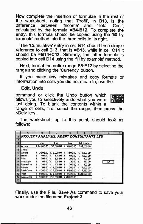
Now complete the insertion of formulae in the rest ofthe worksheet, noting that 'Profit', in B13, is thedifference between 'Income' and 'Total Cost',calculated by the formula =B4 -B12. To complete theentry, this formula should be copied using the 'fill byexample' method into the three cells to its right.

The 'Cumulative' entry in cell B14 should be a simplereference to cell B13, that is =B13, while in cell C14 itshould be =B14+C13. Similarly, the latter formula iscopied into cell D14 using the 'fill by example' method.

Next, format the entire range B6:E12 by selecting therange and clicking the 'Currency' button.

If you make any mistakes and copy formats orinformation into cells you did not mean to, use the

Edit, Undo

command or click the Undo button whichallows you to selectively undo what you werejust doing. To blank the contents within arange of cells, first select the range, then press the<Del> key.

The worksheet, up to this point, should look asfollows:

A 1 B 1 c I D 1 E IF IGIH1 PROJECT ANALYSIS: ADEPT CONSULTANTS LTD2

3 Jan Feb Mar 1st Quarter4 Income £ 14,000 00 £15,000 00 E 16,000 00 £ 45,000 00

5 Costs6 Wages £ 2,000 00 £ 3,000 00 £ 4,030 03 £ 9,000 007 Travel f 400 133 £ 503 03 2 1300 00 f 1,500 008 Pent f 3:0 oo i 330 00 f 330 013 £ 900 009 Heat/lJght £ 150 00 E 200 00 f 133 CO £ 480 00

1 3 1

10 Phone/Fax £ 250 00 £ 300 013 f 350 00 £ 900 0311 Adverts £ 1,100 00 £ 1,200 00 £ 1,300 00 f 3,600 0012 Total Costs £ 4,20000 £ 5,50000 £ 6,68000 £ 16,380 0013 Profit f 9,800 00 £ 9500 00 £ 9,320 00 f 28,620 0014 Cumulatrve E 9,800 00 £19,300 00 £ 28,620 03

15

Finally, use the File, Save As command to save yourwork under the filename Project 3.

46

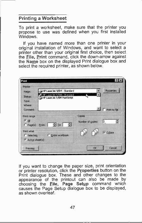
Printing a Worksheet

To print a worksheet, make sure that the printer youpropose to use was defined when you first installedWindows.

If you have named more than cne printer in youroriginal installation o' Windows, and want to select aprinter other than your original first choice, then selectthe File, Print command, click the down-arrow againstthe Name box on the displayed Print dialogue box andselect the required pr nter, as shown below.

Print

Printer -

Naete:

Status:

Type:

Where:

LComment:

-Pri-rt range --r A0r P age(s) Elan: I

Print what

r solectioa r Endre wxkbook

Actixe sheet(s)

Preview I

Copies

Number of Copses;

kooerties

Prnt to hip

OK

Cdate

Cancel

If you want to charge the paper size, print orientationor printer resolution, slick the Properties button on thePrint dialogue box. These and other changes to theappearance of the printout can also be made bychoosing the File, Page Setup command wlichcauses the Page Setup dialogue box to be displayed,as shown overleaf.

47

Page Setup

[Tai ---11 NNW* I 116Kle.1F°cter I Shmt I

Orientatkal

Patrat Ati r unclear* Prrr Preveto

suing c54°^5

a motto: It normal sire

r Et to: It

page(s)wKle by II tel

Paper sge: Ia4 (210 )

Pint weity

Fast page number:

2.]

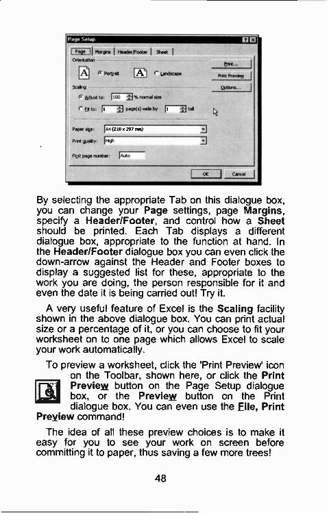
By selecting the appropriate Tab on this dialogue box,you can change your Page settings, page Margins,specify a Header/Footer, and control how a Sheetshould be printed. Each Tab displays a differentdialogue box, appropriate to the function at hand. Inthe Header/Footer dialogue box you can even click thedown-arrow against the Header and Footer boxes todisplay a suggested list for these, appropriate to thework you are doing, the person responsible for it andeven the date it is being carried out! Try it.

A very useful feature of Excel is the Scaling facilityshown in the above dialogue box. You can print actualsize or a percentage of it, or you can choose to fit yourworksheet on to one page which allows Excel to scaleyour work automatically.

To preview a worksheet, click the 'Print Preview' iconon the Toolbar, shown here, or click the PrintPreview button on the Page Setup dialoguebox, or the Preview button cn the Printdialogue box. You can even use the File, Print

Preview command!

The idea of all these preview choices is to make iteasy for you to see your work on screen beforecommitting it to paper, thus saving a few more trees!

48

Enhancing a Worksheet

You can make your work look more professional byadopting various enhancements, such as single anddouble line cell borders, shading certain cells, andadding meaningful headers and footers.

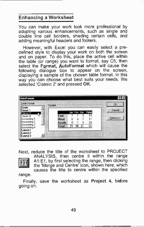
However, with Excel you can easily select a pre-defined style to display your work on both the screenand on paper. To do this, place the active cell withinthe table (or range) you want to format, say 05, thenselect the Format, AutoFormat which will cause thefollowing dialogue box to appear on the screen,displaying a sample of the chosen table format. In thisway you can choose what best suits your needs. Weselected 'Classic 2' and pressed OK.

Autohemai ©©Iable Format

SmpkClasS/C 1

Sample k I

CancelC la tin FN.) ?Aar Total

Classic 3 East 7 7 5 13

ounting 1 West 6 4 7 17.Qpi 10,1S >:

ountrg 23

South 8 7 9 24

Tctal 21 18 214

Colorful 1Colorful 2Colorful 3

Next, reduce the title of the worksheet to PROJECTANALYSIS, then centre it within the rangeA1:E1, by first selecting the range, then clicKingthe 'Merge and Centre' icon, shown here, wiichcauses the title to centre within the specified

range.

Finally, save the worksheet as Project 4, beforegoing on.

49

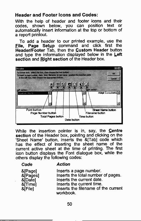
Header and Footer Icons and Codes:With the help of header and footer icons and theircodes, shown below, you can position text orautomatically insert information at the top or bottom ofa report printout.

To add a header to our printed example, use theFile, Page Setup command and click first theHeader/Footer Tab, then the Custom Header buttonand type the information displayed below in the Leftsection and Right section of the Header box.

tirade' E3

To format text: select the text, then choose the font button.To Insert a pep nunber, date, time, fibrorne, or tab name: position the hserton mint

h the edt box, then choose the apse aerie* button.

sector:

Adept Consultan

Font button Sheet Name buttonPage Number button Filename button

Total Pages button Time buttonDate button

While the insertion pointer is in, say, the Centresection of the Header box, pointing and clicking on the'Sheet Name' button, inserts the &[Tab] code whichhas the effect of inserting the sheet name of thecurrent active sheet at the time of printing. The firsticon button displays the Font dialogue box, while theothers display the following codes:

Code Action&[Page] Inserts a page number.&[Pages] Inserts the total number of pages.&[Date] Inserts the current date.&[Time] Inserts the current time.&[File] Inserts the filename of the current

workbook.

50

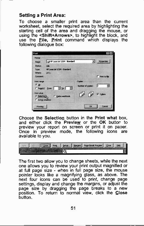
Setting a Print Area:To choose a smaller print area than the currentworksheet, select the required area by highlighting thestarting cell of the area and dragging the mouse, orusing the <Shift+A-rows>, to highlight the block, 3nduse the File, Print command which displays thefollowing dialogue box:

Punt 0E1Printer

Nom;LAW Laser:et Tirsel 9andeed

Rat= We

Type: TV LaserJet Vita - Standard

Where: LPTI:

Comment:

Print range

Ej

r Pacte(s) Erom:

Print what

r Actrop sheet(s)

Jet,

thp, I

C [stirs workbook

r Pelt to file

Copies

Mester el copies: l

LJ [1; Collate

r«I Cancel

Choose the Selection button in the Print what box,and either click tt-e Preview or :he OK buttor topreview your report on screen or print it on paper.Once in preview mode, the following icons areavailable to you.

The first two allow y0:._1 to change sheets, while the nextone allows you to review your print output magnified orat full page size - when in full page size, the mousepointer looks like -nagnifying glass, as above. Thenext four icons can be used to print, change pagesettings, display and change the margins, or adjust thepage size by dragging the page breaks to a newposition. To return to normal view, click the Closebutton.

51

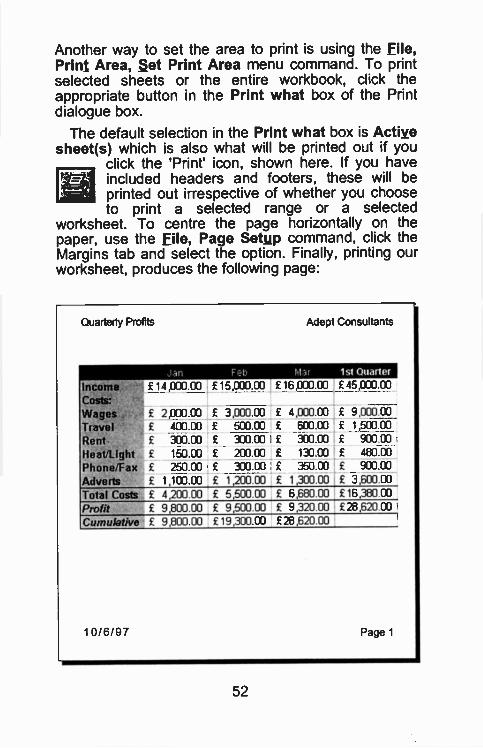
Another way to set the area to print is using the File,Print Area, Set Print Area menu command. To printselected sheets or the entire workbook, click theappropriate button in the Print what box of the Printdialogue box.

The default selection in the Print what box is Activesheet(s) which is also what will be printed out if you

click the 'Print' icon, shown here. If you haveincluded headers and footers, these will beprinted out irrespective of whether you chooseto print a selected range or a selected

worksheet. To centre the page horizontally on thepaper, use the File, Page Setup command, click theMargins tab and select the option. Finally, printing ourworksheet, produces the following page:

Quarterly Profits Adept Consultants

to.:it 1st Ouarter

Income £14,000 00 £15,000.00 £16,000.00 £45,000.00

Costs:Wages £ 2,000 00 £ 3,000 00 £ 4,000.00 £ 9,000.00Travel £ 400 00 £ 500.00 £ 600.00 £ 1,500.00Rent £ 300.00 £ 300.00 £ 300 00 £ 900.00

Heat/Light £,...._150.00 £ 200.00 £ 130.00 £ 480.00

Phone/Fax £ 250.00 £ 300 00 £ 350.00 £ 900.00

Adverts £ 1,100.00 £ 1,200.00 £ 1,300.00 £ 3,600.00Total Costs £ 4,200.00 £ 6,500.00 £ 6,680.00 £16,380.00

Profit £ 9,800.00 £ 9,500.00 £ 9,320.00 £28,620.00

Cumulative £ 9,800.00 £19,300.00 £28,620.00

10/6/97 Page 1

52

3 -Dimensional Worksheets

In Excel 97, a Workbook is a 3 -dimensional file madeup with a series of =tat 2 -dimensional sheets stacked'on top of each other'. Each sheet is the same size,and in itself, behaves the same as t-ie more ordinaryworksheets. As mertioned previously, each separatesheet in a file has its own Tab identifier at the bottom ofthe screen. Ranges can be set to span severaldifferent sheets to build up 3 -dimensional blocks ofdata. These blocks can then be manipulated, copied,or moved to other locations in the file. A cell canreference any other cell in the file, no matter whatsheet it is on, and an extended range of functions canbe used to process these 3 -dimensional ranges.

Manipulating Ranges:The best way to demonstrate a new idea is :o workthrough an example - we will use the worksheet saved

under Project 4. Next, start Excel, use the Foe,Open command, or click the File Open icon,and select Project 4. On pressing <Enter>, theworksheet should be displayec on the screen as

shown on the facing page.

Copying Sheets in a Workbook:We will now fill another three sheets behind the presentone, in order to include informaticn about ADE DTConsultants' trading during the other three quarters ofthe year. The easiest way of doing this is by copyingthe information in Sheet1 , including the formatting andthe entered formulae, onto the other three sheets, thenedit the numerical information in these appropriately.

To simplify this ope-ation, Excel has a facility wh challows you to copy a sheet into a workbook. There aretwo ways of doing this: (a) with the mouse, or (b) usingthe menus.

53

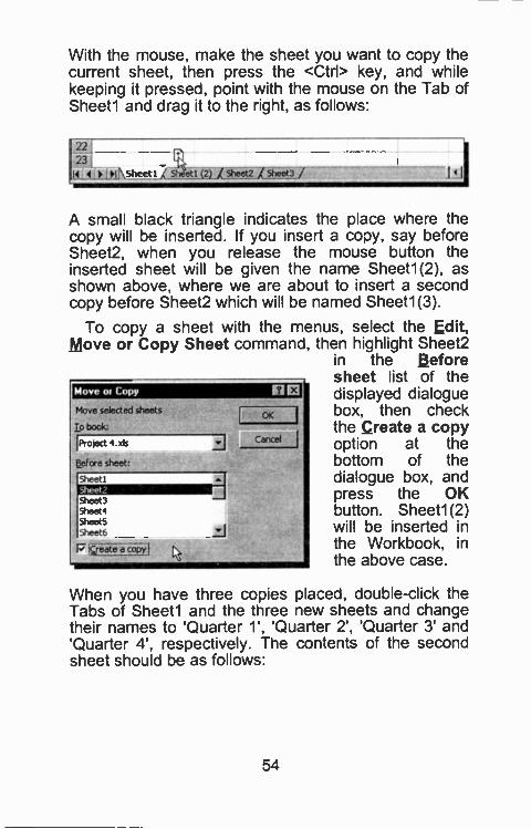
With the mouse, make the sheet you want to copy thecurrent sheet, then press the <Ctrl> key, and whilekeeping it pressed, point with the mouse on the Tab ofSheet1 and drag it to the right, as follows:

22.23;

14 41iLM N5heet 1 2- 1 ()_L5hept3 SheetA

A small black triangle indicates the place where thecopy will be inserted. If you insert a copy, say beforeSheet2, when you release the mouse button theinserted sheet will be given the name Sheet1(2), asshown above, where we are about to insert a secondcopy before Sheet2 which will be named Sheet1(3).

To copy a sheet with the menus, select the Edit,Move or Copy Sheet command, then highlight Sheet2

in the Beforesheet list of thedisplayed dialoguebox, then checkthe Create a copyoption at thebottom of thedialogue box, and

Sheet 3press the OK

Sheet 4 button. Sheet1(2)ire _:J will De inserted in

id N the Workbook, inthe above case.

Move ot Copy

Move selected sheets

Lo book:

!Project 4 .xk

Wore sheet:

Sheet 1

=_I

OK

Cancel

When you have three copies placed, double-click theTabs of Sheet1 and the three new sheets and changetheir names to 'Quarter 1', 'Quarter 2', 'Quarter 3' and'Quarter 4', respectively. The contents of the secondsheet should be as follows:

54

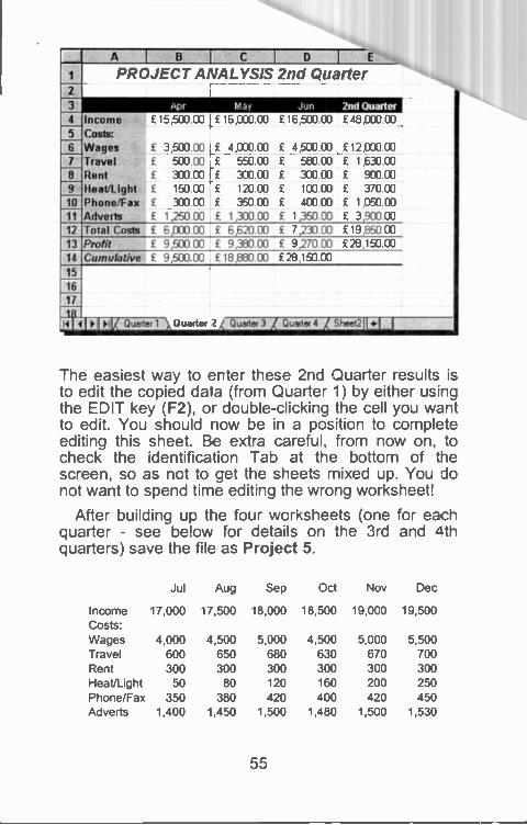
A

1 PROJECT ANALYSIS

Apr May

2nd Quarter

Jun 2nd Ouarte4

2

3

4 Income £15,500 CIO £ 16,000 00 £ 16500 00 £ 48,000 00

5 Costs:6 Wages £ 3,503.00 £ 4,000.00 £ 4,500.00 £12,000 00

7 Travel £ 500 00 £ 550.00 £ 580.00 £ 1,630 CO

8 Rent £ 300 CO £ 333.00 £ 300.00 £ 903 039 Heat/Light £ 150 00 £ 120 00 £ 100 00 £ 370 03

10 Phone/Fax £ 300.00 £ 350.00 £ 400 00 £ 1,050 CO

11 Adverts £ 1,250.00 £ 1,300.03 £ 1,350.00 £ 3,900 00

12 Total Costs £ 6,000 00 £ 6,62000 £ 7,2313 00 £ 19,850 00

13 Profit £ 9500 00 £ 9,380 00 £ 9,270 00 28,150 00

14 Cumulative £ 9,500 00 £ 18 880.00 £28 150 00

15

16

17

11111/ Quarter 1 \ Quarter 2,( Quarter 3 Puma 4 Sheet211.I I

The easiest way to erter these 2nd Quarter results isto edit the copied data (from Quarter 1) by either usingthe EDIT key (F2), o- double-clicking the cell you wantto edit. You should now be in a position to completeediting this sheet. Be extra careful, from now on, tocheck the identification Tab at the bottom of thescreen, so as not to get the sheets mixed up. You donot want to spend time editing the wrcng worksheet!

After building up the four worksheets (one for eachquarter - see below for details on the 3rd and 4thquarters) save the file as Project 5.

Jul Aug Sep Oct Nov Dec

Income 17,000 17,500 18,000 18,500 19,000 '9,500Costs:Wages 4,000 4,500 5,000 4,500 5,000 5,500Travel 600 650 680 630 670 700Rent 300 300 300 300 300 300Heat/Light 50 80 120 160 200 250Phone/Fax 350 380 420 400 420 450Adverts 1,400 1,450 1,500 1,480 1,500 1,530

55

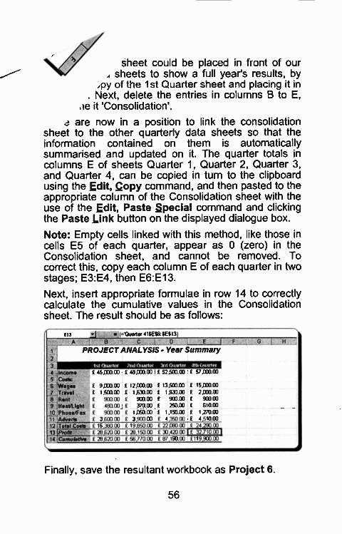
sheet could be placed in front of our, sheets to show a full year's results, by

,py of the 1st Quarter sheet and placing it in. Next, delete the entries in columns B to E,

'le it 'Consolidation'.

are now in a position to link the consolidationsheet to the other quarterly data sheets so that theinformation contained on them is automaticallysummarised and updated on it. The quarter totals incolumns E of sheets Quarter 1, Quarter 2, Quarter 3,and Quarter 4, can be copied in turn to the clipboardusing the Edit, Copy command, and then pasted to theappropriate column of the Consolidation sheet with theuse of the Edit, Paste Special command and clickingthe Paste Link button on the displayed dialogue box.

Note: Empty cells linked with this method, like those incells E5 of each quarter, appear as 0 (zero) in theConsolidation sheet, and cannot be removed. Tocorrect this, copy each column E of each quarter in twostages; E3:E4, then E6:E13.

Next, insert appropriate formulae in row 14 to correctlycalculate the cumulative values in the Consolidationsheet. The result should be as follows:

E13fi I.'Quarter 4'$E$6 SES13)A , B C

PROJECT ANALYSIS2

0 E IF 0 H

- Year Summary

3 1st Quarter 2nd O,wter Vii (Miner 4th Oliartmr

;Income E 4500000 f 48,030 00 52,500 00 E 570133 00

5 Costs6 'Wages f 9,00000 f 12,000 00 £ 1350000 f 15.000 00

7 Travel f 1500 00 f 1,630 CO 1,933 00 f 2000 008 Rent f 900 00 f 900 00 f 900 CO f 903 00

9 HeatiLlght f 48000 f 37000 f 25003 f 6100010 Rhone/Fax £ 900 00 £ 1,05000 E 1,15000 f 1,2700011 Adverts £ 3,600 CO f 3,900 00 f 4.350 00 E 4,510 Lc

12 Total Costs £ 16,330 CO £ 19650 00 £ 22Deo 00 24 290 00

13 [Pratt £ 2862000 f 2815003 f 33 420 00 1E 32.71000114 iCumukatIve f 28 620 03 f 56,770 CO 87,190 00 £119,900 00

Finally, save the resultant workbook as Project 6.

56

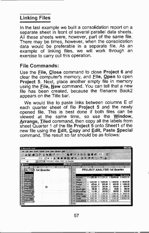
Linking Files

In the last example we built a consolidation report on aseparate sheet in front of several parallel data sheets.All these sheets were, however, part of the same file.There may be times, however, whe'i the consolidationdata would be preferable in a separate file. As anexample of linking files, we will work through anexercise to carry out this operation.

File Commands:Use the File, Close command to close Project 6 andclear the computer's memory, and File, Qpen to cpenProject 5. Next, p ace another empty file in memoryusing the File, New command. You can tell that a newfile has been created, because the filename Book2appears on the Title bar.

We would like to paste links between columns E ofeach quarter sheet of file Project 5 and the newlyopened file. This is best done if both files car beviewed at the same time, so use the Window,Arrange, Tiled command, then copy all the labels 'rpmsheet Quarter 1 of :he file Project 5 onto Sheet1 o: thenew file using the Edit, Copy and Edit, Paste specialcommand. The result so far should be as follows:

CM LA 13. Ire. 46.4 imis Oct. I.A. isOriOat 4t CC' - r tl tit "."' .0rr zg is is a Ili CP /t eS tf6 8, Z1..1

.1 PNWECT MAYS:,' w.,1

0 C E

1st Quarter

O

-A 6.9A B C ) E

1 PROJECT ANALYSIS 1st Quarter2

3 11.1111.111.11111111=I Income f 14 00 00 15= CO 16,403 00 f46E00 00S LAMA6 992. 7 1.71 00 3071 03 50 CO f 9®007 Tr 1..4 f AO CO 4:0 00 60000 I 1 433 CO

Rani f 37 00 3M CO 3C0 03 ( 900 133

9 NalA.Ight f 1M 03 200 CO 33 00 f 460 00

10 Phone/Fox I 24) 00 333 CD 360 CO I 930 013

11 A.1.94 1,1C0 CO IA) CO 000 CO f 9803 OC

12 To141 Cow f .,23300 5'3000 6,66000 (1631300013 Profit f 9 sco CIO 94:0 00 9020 CO ( 2E100 CIC

tf C6IIIMANIVII f oal)CC 19,330 OD 213520 OD

16

57

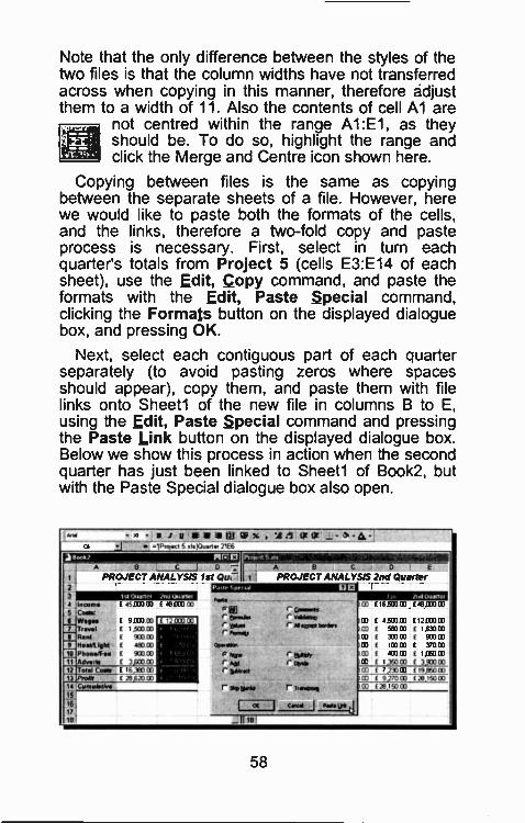
Note that the only difference between the styles of thetwo files is that the column widths have not transferredacross when copying in this manner, therefore adjustthem to a width of 11. Also the contents of cell Al are

not centred within the range Al:El , as theyshould be. To do so, highlight the range andclick the Merge and Centre icon shown here.

Copying between files is the same as copyingbetween the separate sheets of a file. However, herewe would like to paste both the formats of the cells,and the links, therefore a two -fold copy and pasteprocess is necessary. First, select in turn eachquarter's totals from Project 5 (cells E3:E14 of eachsheet), use the Edit, Copy command, and paste theformats with the Edit, Paste Special command,clicking the Formats button on the displayed dialoguebox, and pressing OK.

Next, select each contiguous part of each quarterseparately (to avoid pasting zeros where spacesshould appear), copy them, and paste them with filelinks onto Sheetl of the new file in columns B to E,using the Edit, Paste Special command and pressingthe Paste Link button on the displayed dialogue box.Below we show this process in action when the secondquarter has just been linked to Sheetl cf Book2, butwith the Paste Special dialogue box also open.

u meow ;lox . '44 flfOf _ . =1Prara 5 aliClutellit 7116

1111161111110111111111A 8 C D7

PROJECT ANALYSIS 1st Qu.2

3 Ir=r2fr3214 Inca Ina I 45.00000 I 1603000

5 Col:8 Wain

TravelRaniilita41.19141

Phone FatAdvents

9.003 CO

E 1 503 CO

903 CU

f 480 CO

f 900 CO70 CO

Total Coal. 1 16 130 CC

Palle cp ruol

r !Palar Yet.r My rtr

CDnrlm

r. licrar adp4- Sanaa

r sotorie

16

58

PROJECT ANALYSTS 2nd Quarter

wklIfoo

Maacent

CO 11650003011.f101

48 030 00

CO f (MOOD 1203000CO I 50303 1.6300DCO f 333 CO 933 LE

CZ1 f 10000 370 00CC f 40300 1,06000CC f 1 CO 3 90000

Fl I 7,73118 1903,85000 I 9 70 CO 213 150 CO

CO E7B150m

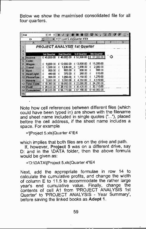
Below we show the maximised consolidated file for allfour quarters.

Anal

E4

- e t WU Di SIR % e2 or si<_ sii.1Poject 5 xlsjOuarter 41E4

A 131C1 023

PROJECT ANALYSIS 1st Quarter

1st °limier 2nd Owls ten 3rd Ouartet 4th Quartet

4 Income £ 45,030 00 £ 48= 00 £ 52,500.00 £ 57,000 00

5 ;Costa6 ,Wages £ 9,000.00 f 12900.00 f 13,500 00 £ 15,.000.00

7 /Travel f 1,500 00 f 1,1390.130 £ 1930.00 £ 2,030.00

a Rent £ 930 03 930.00 f 930.00 £ 900 CO

9 iHost/Light £ 193 M f 370 00 f 250 00 f 610.00

101Phona/Fax 900.013 f 1950E33 £ 1,15000 £ 1270.00

11 ;Adverts f 3,600.00 £ 3,900.00 f 4,350.03 f 1,510 M

12 !Total Costs f 16,330 03 f 19,1350.1:0 f 22030.00 £ 24290.0013 'Profit E 26,620.00 f 26,150.00 £ 33,4213.03 £ 32,710 00

14 Cumulative £ 33,620 00 £ 56,770.00 £ 87,190 00 f '19,900.03

15

Note how cell references between different files (whichcould have been typed in) are shown with the filenameand sheet name included in single quotes ('...'), placedbefore the cell address, if the sheet name includes aspace. For example

='[Project 5.xls]Quarter 41E4

which implies that bcth files are on the drive and path.If, however, Project 5 was on a different drive, say

D: and in the \DATA folder, then the above formulawould be given as:

='D:\DATA\[Project 5.xls]Quarter 41E4

Next, add the appropriate formulae in row 14 tocalculate the cumulative profits, and change the widthof column E to 11.5 to accommodate the rather largeyear's end cumulative value. Finally, change thecontents of cell Al from 'PROJECT ANALYSIS 1stQuarter' to 'PROJECT ANALYSIS - Year Summary',before saving the linked books as Adept 1.

59

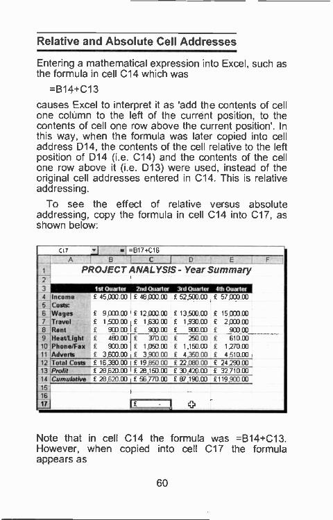
Relative and Absolute Cell Addresses

Entering a mathematical expression into Excel, such asthe formula in cell C14 which was

=B14+C13

causes Excel to interpret it as 'add the contents of cellone coltjmn to the left of the current position, to thecontents of cell one row above the current position'. Inthis way, when the formula was later copied into celladdress D14, the contents of the cell relative to the leftposition of D14 (i.e. C14) and the contents of the cellone row above it (i.e. D13) were used, instead of theoriginal cell addresses entered in C14. This is relativeaddressing.

To see the effect of relative versus absoluteaddressing, copy the formula in cell C14 into C17, asshown below:

C17 =617+C16

A

A I D

- Year Summary1 PROJECT ANALYSIS

3 1st °natter 2ritl Quarter 3rd Ouarter 4th Ottarter4 Income 45,000.00 f 48,000.00 f 52,500.00 £ 57,000.005 Costs:6 Wages £ 9,000.00 12,000.00 f 13500.130 £ 15 8C10.007 Travel £ 1,500.00 £ 1,630.00 £ 1,930.00 £ 2.000.008 Rent £ 900.00 £ 900.00 £ 900.00 £ 900.009 Heat/Light £ 480.00 370.00 £ 250.00 £ 610.0010 Phone/Fax £ 900.00 £ 1,050.00 £ 1,150.00 £ 1,270.0011 'Adverts £ 3,600.00 3,900.00 £ 4,350.00 £ 4510.0012 Total Costs £ 16,380.00 f 19,850.00 £ 22,0130.00 £ 24 293.0013 Profit 28620.00 f 28,150.00 33420.00 E 32.710 0014 Cumulative 28,620.00 £ 56,770.00 f 87,190.00 £119,930.0015

Note that in cell C14 the formula was =B14+C13.However, when copied into cell C17 the formulaappears as

60

=B17+C16

because it has been interpreted as -elative addressing.In this case, no value appears in cell C17 because weare attempting to add two blank cells.

Now change the formula in C14 by editing it to

=$B$14+$C$13

which is interpreted as absolute addressing. Copyingthis formula into cell C17 calculates the correct result.Highlight cell C17 and observe the cell references in itsformula; they have not changed from those of cell C14.

The $ sign must prefix both the column referenceand the row reference. Mixed cell addressing ispermitted; as for example when a column addressreference is needed to be taken as absolute, while arow address reference is needed to be taken asrelative. In such a case, the column letter is prefixed bythe $ sign.

When building an absolute cell reference in a

formula, it is easier to select the cell with the mcusepointer and keep pressing the F4 key until the correct $prefix is set.

Freezing Panes on Screen

Sometimes there might be too much information onscreen and attempting to see a certain part of a sheetmight cause the labels associated with that informationto scroll off the screen.

To freeze column (or row) labels of a worksheet onscreen, move the cell pointer to the right (or below) thecolumn (or row) which you want to freeze, and use the

Window, Freeze Panescommand. Everything to the left of ,'or above) the cellpointer will freeze on the screen.

61

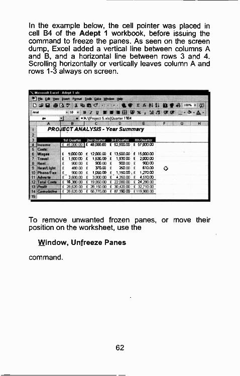
In the example below, the cell pointer was placed incell B4 of the Adept 1 workbook, before issuing thecommand to freeze the panes. As seen on the screendump, Excel added a vertical line between columns Aand B, and a horizontal line between rows 3 and 4.Scrolling horizontally or vertically leaves column A androws 1-3 always on screen.

\ Moves.,It Ecel Adept 1 als

111 Els Edit V.'. {mart Pirmit 100111 (WA Widow yelp

Cal; ei V' X ia IS 4 es* f.. ii I. ill ft '°°°'And 10

b4 si =A / u Ili al 11 E8 CP Ir - a. A -

Wrojeci 5 41s1Ouarter 11E4

A

PROJECT2

3

B C 0

Summary

Beatles 41hOuarler

ANALYSIS - Year

lot Wader 2m1Otiartes 3rd4 Income I. 45 WO 00 48,000 CD 52,500 00 57,003 005 Cost::6 Wages 2 9,000 00 £ 12.000 00 f 13,500 03 £ 15,000 007 Travel 2 1500 00 f 1530 00 f 1,933 CO f 2.000 008 Rent f 903 1313 f 900 03 £ 903 CO f 900 009 Heal/tight f 483 00 f 370 00 2 25003 f 6100010 Phone/Fes £ 903 00 £ 1,050 00 1,150 00 £ 1270 0011 Adverb f 3,600 CO f 3,900 00 f 4 350 CO f 4,5100012 Total Costs f 16,360 00 f 19,1350 03 f 22000 CO £ 24290 01313 F'rolh f 33,620 00 £ 213,150133 f 33,420 03 f 32,710 0014 Cumulative f 213 620 00 f 56 770 00 f 87.190 00 f 119 900 0015

To remove unwanted frozen panes, or move theirposition on the worksheet, use the

Window, Unfreeze Panes

command.

62

4. SPREADSHEET CHARTS

Excel allows information within a worksheet to berepresented in graphical form, which makes data moreaccessible to non -expert users who might no: befamiliar with the spreadsheet format. The sayirg 'apicture is worth a thousand words', applies ecually wellto charts and figures.

The package allows the use of several chart andgraph types, including area, bar, column, line,doughnut, radar, XY, pie, combination, and several 3-Doptions of these charts. In all, Excel allows fourteendifferent types of charts, with almost 100 pre -definedformats, which can be selected by using theappropriate icon. These are made available to youonce you have selected the data you want to chart andclicked on the Chart Wizard button on the toolbar.

Charts (you can lave several per worksheet) cal bedisplayed on screen at the same time as the worksheetfrom which they were derived, sirce they appear intheir own 'chart' frame and can be embeddedanywhere on a wcrksheet. Furthermore, they can besent to an appropriate output device, such as a plotteror printer. Althougt this charting module rivals astandalone graphics package, and one could write aseparate book on it, an attempt will be made to presentits basics, in the space available within this book.

Preparing for a Column Chart

In order to illustrate some of the graphing capabilitiesof Excel, we will now plot the income of the consu tingcompany we discussed in the Project 6 file. However,before we can go on, you will need to complete theentries for the last two quarters of trading of the AdeptConsultants' example, if you haven't already cone so -see end of previous chapter.

63

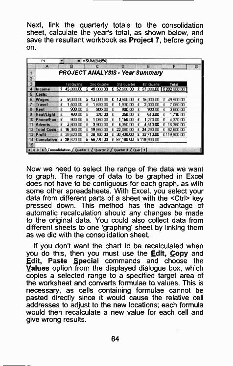
Next, link the quarterly totals to the consolidationsheet, calculate the year's total, as shown below, andsave the resultant workbook as Project 7, before goingon.

F1 zi l =SUM(B4 E4)0 ! C 0 E

PROJECT ANALYSIS - Year Summary2!3 I ,i Ou:grief 20.: Ch.:411,r 3rd ..wa 1.?.r 411- OLarter Total4 Income £ 45 000 00 f 48 000 00 £ 52,5[10 00 £ 57,000 03 1 202 500 005 Costs6 Wages f 9,000 00 £ 12,000 00 f 13,500 00 £ 15,000 00 f 49,500 007 Travel £ 1,500 00 f 1.630 00 £ 1,930 00 f 2,000 00 i 7,060 008 Rent £ 900 00 £ 900 00 £ 903 03 1 903 00 i 3,600 009 Heat/Light f 480 00 £ 370 03 £ 250 00 £ 610 03 i 1,710 CC

10 Phone/Fax f 90000 £ 1,05000 £ 1,15000 1 1270 00 i 4.3700011 Advert f 3,603 00 £ 3,930 00 f 4,350 03 1 4,510 03 1 16,360 0012 Total Costs £ 16,330 00 £ 19,850 00 £ 22,080 CO £ 24,2913 00 1 82.600 0013 Profit £ 28,620 00 £ 28,150 00 £ 33,420 CO £ 32/10 00 1 119900 0314 Cumulative £ 28,620 00 £ 56,770 00 £ 87,190 00 £119,900 0315

N I rM \ Consolidation / Quarter 1 Rutter 2 i Quarter 3 7Q.;14 I I

Now we need to select the range of the data we wantto graph. The range of data to be graphed in Exceldoes not have to be contiguous for each graph, as withsome other spreadsheets. With Excel, you select yourdata from different parts of a sheet with the <Ctrl> keypressed down. This method has the advantage ofautomatic recalculation should any changes be madeto the original data. You could also collect data fromdifferent sheets to one 'graphing' sheet by linking themas we did with the consolidation sheet.

If you don't want the chart to be recalculated whenyou do this, then you must use the Edit, Copy andEdit, Paste Special commands and choose theValues option from the displayed dialogue box, whichcopies a selected range to a specified target area ofthe worksheet and converts formulae to values. This isnecessary, as cells containing formulae cannot bepasted directly since it would cause the relative celladdresses to adjust to the new locations; each formulawould then recalculate a new value for each cell andgive wrong results.

64

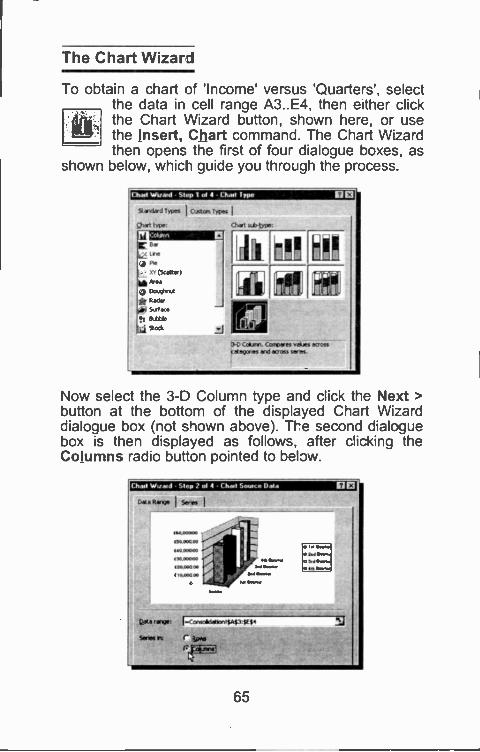
The Chart Wizard

To obtain a chart of 'Income' versus 'Quarters', selectthe data in cell range A3..E4, then either clickthe Chart Wizard button, shown here, or usethe Insert, Chart command. The Chart Wizardthen opens the first of four dialogue boxes, as

shown below, which guide you through the process.

(11.111 W1,91(1 ',el. I of 4 I had type IDStandard Tn. I Clacton Types I

glut Me:

Lie)

oftXY (Scatter)

Area

Dauctrat(a, Radar

SolaceIt &Atte

Stork

Chart

ii 01 liM

DO Gamut Carpus values sawslutists.; and across was.

Now select the 3-D Column type and click the Next >button at the bottom of the displayed Chart Wizarddialogue box (not shown above). The second dialoguebox is then displayed as follows, after clicking theColumns radio button pointed to below.

Chas, W,rel Step 7 of 4 - rhArl Sava, Date noDaRing I sem. I

Qata rang,: kCOrriSiddlOr1.1.43 11$.

Sores Pr r iYae7.41

65

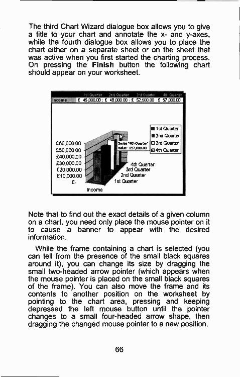
The third Chart Wizard dialogue box allows you to givea title to your chart and annotate the x- and y-axes,while the fourth dialogue box allows you to place thechart either on a separate sheet or on the sheet thatwas active when you first started the charting process.On pressing the Finish button the following chartshould appear on your worksheet.

I' r ri,,r1r, 411 .:,u4rler

Income 45,000 00 E 48,000 00 £ 52,500 00 £ 57000 00

£60,000 00

£50,000 00£40,000 00£30,000 00£20,000 00£10,000.00

E-

!es"4thQuccter.Value: £57,000.00

01

Income

Ea 1st Quarter

IN 2nd Cuarter

0 3rd Quarter

04th Quarter

4th Quarter3rd Quarter

2nd Quarter1st Quarter

Note that to find out the exact details of a given columnon a chart, you need only place the mouse pointer on itto cause a banner to appear with the desiredinformation.

While the frame containing a chart is selected (youcan tell from the presence of the small black squaresaround it), you can change its size by dragging thesmall two -headed arrow pointer (which appears whenthe mouse pointer is placed on the small black squaresof the frame). You can also move the frame and itscontents to another position on the worksheet bypointing to the chart area, pressing and keepingdepressed the left mouse button unti' the pointerchanges to a small four -headed arrow shape, thendragging the changed mouse pointer to a new position.

66

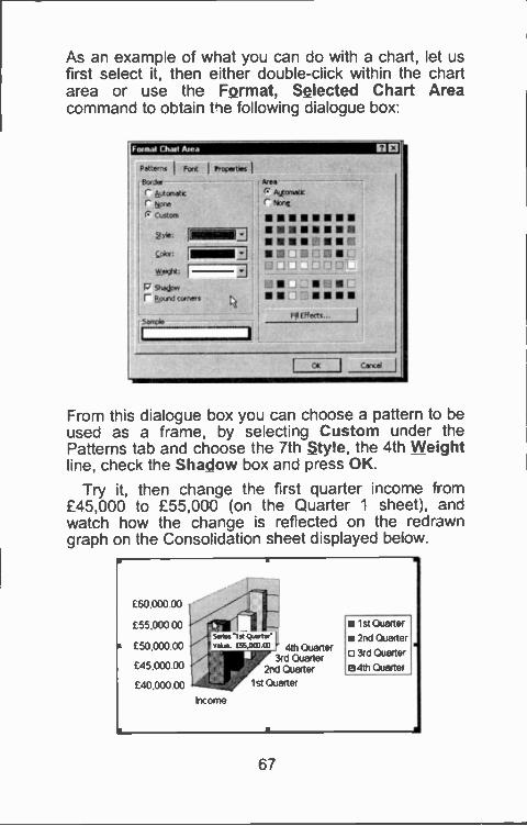
As an example of wnat you can do with a chart, let usfirst select it, then either double-click within the chartarea or use the Format, Selected Chart Areacommand to obtain he following dialogue box.

Fantal [hail Area

Patterns I Font I FropertM I

Border

Automatic

r jone

r custom

2tyle:

IMO=&.cht:

p- Shodow 111

r Round corners

Semooie

HI Effects

OK

From this dialogue box you can choose a pattern to beused as a frame, by selecting Custom u'ider thePatterns tab and cl-oose the 7th Style, the 4th Weightline, check the Shadow box and press OK.

Try it, then change the first quarter income from£45,000 to £55,000 (on the Quarter 1 sheet), andwatch how the change is reflected on the redrawngraph on the Consolidation sheet displayed be ow.

£60.000 00

155.000 00

150.000 00

£45.000 00

140.000 00

Income

4M Quarter3rd Quarter

2nd Quarter

1st Quarter

0 1st Quarter

II 2nd Quarter

0 3rd Quarter

04th Quarter

67

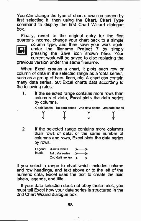
You can change the type of chart shown on screen byfirst selecting it, then using the Chart, Chart Typecommand to display the first Chart Wizard dialoguebox.

Finally, revert to the original entry for the firstquarter's income, change your chart back to a simple

column type, and then save your work againunder the filename Project 7 by simplypressing the Save icon shown here. Yourcurrent work will be saved to disc replacing the

previous version under the same filename.

When Excel creates a chart, it plots each row orcolumn of data in the selected range as a 'data series',such as a group of bars, lines, etc. A chart can containmany data series, but Excel charts data according tothe following rules:

1. If the selected range contains more rows thancolumns of data, Excel plots the data seriesby columns.X-axis labels 1st data series 2nd data series 3rd data series

2. If the selected range contains more columnsthan rows of data, or the same number ofcolumns and rows, Excel plots the data seriesby rows.

Legendlabels

X-axis labels1st data series2nd data series

If you select a range to chart which inc udes columnand row headings, and text above or to the left of thenumeric data, Excel uses the text to create the axislabels, legends, and title.

If your data selection does not obey these rules, youmust tell Excel how your data series is structured in the2nd Chart Wizard dialogue box.

68

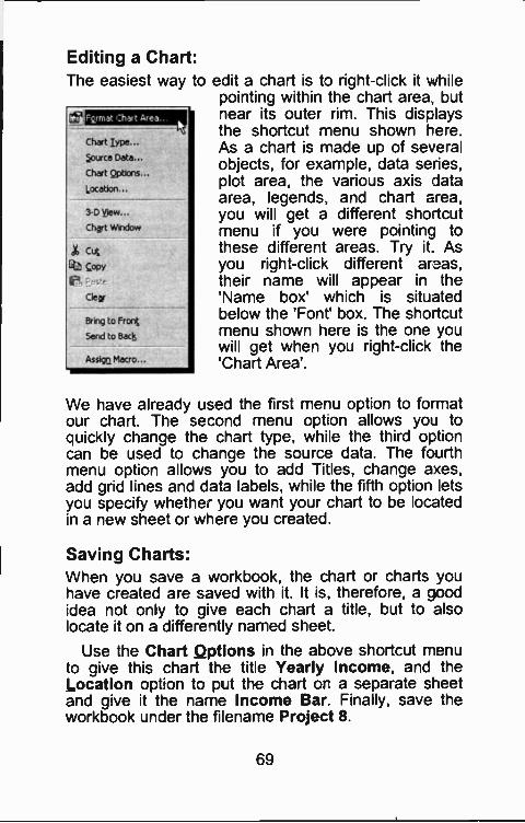
Editing a Chart:The easiest way tc edit a chart is to right -click it while

pointing within the chart area butnear its outer rim. This displaysthe shortcut menu shown here.As a chart is made up of severalobjects, for example, data series,plot area, the various axis iataarea, legends and chart area,you will get a different sho-tcutmenu if you were pointing tothese different areas. Try it. Asyou right -click different areas,their name will appear in the'Name box' which is situatedbelow the 'Font' box. The shortcutmenu shown here is the one youwill get when you right -click the'Chart Area'.

&11131111=1Mchart Ira..2ource Data...

Chart Qptions...

Location...

3-0 View...

Chart Window

A CutE copyti

Cleor

Bring to Front

Send to Back

Assign Macro...

We have already used the first menu option to formatour chart. The second menu opt on allows you toquickly change the chart type, while the third optioncan be used to change the source data. The fourthmenu option allows you to add Titles, change a:<es,add grid lines and data labels, while the fifth option letsyou specify whethe- you want your chart to be locatedin a new sheet or where you created.

Saving Charts:When you save a workbook, the chart or charts youhave created are saved with it. It is. therefore, a goodidea not only to give each chart a title, but to alsolocate it on a differeitly named sheet.

Use the Chart Options in the above shortcut menuto give this chart the title Yearly Income, and theLocation option to put the chart or a separate sheetand give it the name Income Bar. Finally, save theworkbook under the filename Project 8.

69

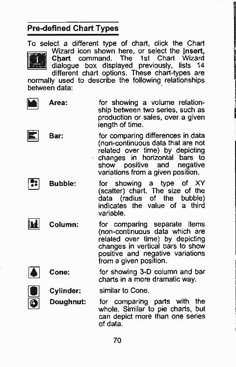
Pre -defined Chart Types

To select a different type of chart, click the ChartWizard icon shown here, or select the Insert,Chart command. The 1st Chart Wizarddialogue box displayed previously, lists 14different chart options. These chart -types are

normally used to describe the following relationshipsbetween data:

Area:

Bar:

for showing a volume relation-ship between two series, such asproduction or sales, over a givenlength of time.

for comparing differences in data(non -continuous data that are notrelated over time) by depictingchanges in horizontal bars toshow positive and negativevariations from a given position.

e*i Bubble: for showing a type of XY(scatter) chart. The size of thedata (radius of the bubble)indicates the value of a thirdvariable.

la Column: for comparing separate items(non -continuous data which arerelated over time) by depictingchanges in vertical oars to showpositive and negative variationsfrom a given position.

Cone: for showing 3-D column and barcharts in a more dramatic way.

Cylinder: similar to Cone.

Doughnut: for comparing parts with thewhole. Similar to pie charts, butcan depict more than one seriesof data.

4

S

70

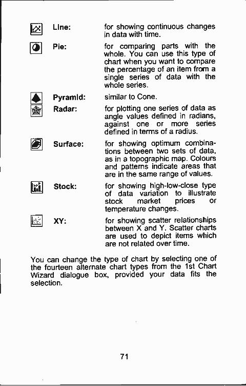
1WLine: for showing continuous chargesin data with time.

Pie: for comparing parts with thewhole. You can use this type ofchart when you want to comparethe percentage of an item from asingle series of data with thewhole series.

Pyramid: similar to Cone.

Radar: for plotting one series of data asangle values defined in radians,against one or more seriesdefined in terms of a radius.

Surface: for showing optimum combina-tions between two sets of data,as in a topographic map Coloursand patterns indicate areas thatare in the same range of values.

Stock: for showing righ-low-close typeof data variation to illust-atestock market prices ortemperature changes.

XY: for showing scatter relationshipsbetween X and Y. Scatter chartsare used to depict items whichare not related over time.

You can change the type of chart by selecting one ofthe fourteen alternate chart types from the 1st CartWizard dialogue box, provided your data fits theselection.

71

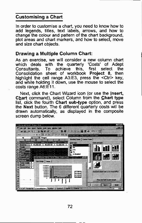
Customising a Chart

In order to customise a chart, you need to know how toadd legends, titles, text labels, arrows, and how tochange the colour and pattern of the chart background,plot areas and chart markers, and how to select, moveand size chart objects.

Drawing a Multiple Column Chart:As an exercise, we will consider a new column chartwhich deals with the quarterly 'Costs' of AdeptConsultants. To achieve this, first select theConsolidation sheet of workbook Project 8, thenhighlight the cell range A3:E3, press the <Ctrl> key,and while holding it down, use the mouse to select thecosts range A6:E11.

Next, click the Chart Wizard icon (or use the Insert,Chart command), select Column from the Chart typelist, click the fourth Chart sub -type option, and pressthe Next button. The 6 different quarterly costs will bedrawn automatically, as displayed in the compositescreen dump below.

12 Total Comb13 Psofit14 Lonotiotivo15

16

4-st V.It \.1.0006.! UPootPlaofk. 1 6t4P3W 1 glOttikst

72

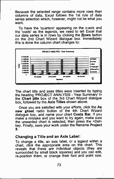
Because the selected range contains more rows thancolumns of data, Excel follows the 1st rule of dataseries selection which, however, m'ght not be what youwant.

To have the 'qt_arters' appearing on the x-axis andthe 'costs' as the legends, we need to tell Exce thatour data series is in rows by clicking the Rows buttonon the 2nd Chart Wizard dialogue box. Immed atelythis is done the column chart changes to:

C16 OCO 00

(1400000(12,0:0 00C10000 CO

CO,CO3 CO

C6,000 CO

(4,000 00OCO 00

it Quads,

PROJECT ANALYSIS Y.., Summary

2nd Owls, 3n1 Curter

Cluart.r

411 Quarter

Wases Tram,O ft^O Mee A.411

Movie: Ad,.

The chart title and axes titles were inserted by typingthe heading 'PROJECT ANALYSIS - Year Summary' inthe Chart title box of the 3rd Chart Wizard dialoguebox, followed by the Axis Titles shown above.

Once you are satisfied with your efforts, click the Asnew sheet radio button of the 4th Chart W zarddialogue box, and name your chart Costs Bar. If youmake a mistake and you want to try again, make surethe unwanted chart is selected, then press the <Del>key. Finally, save your work under the filename Project9.

Changing a Title and an Axis Label:To change a title, an axis label, o- a legend within achart, click the appropriate area on the chart. Thisreveals that these are individual objects (they aresurrounded by small black squares) and you can edit,re -position them, or change their font and point size.

73

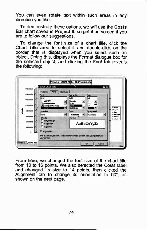
You can even rotate text within such areas in anydirection you like.

To demonstrate these options, we will use the CostsBar chart saved in Project 9, so get it on screen if youare to follow our suggestions.

To change the font size of a chart title, click theChart Title area to select it and double-click on theborder that is displayed when you select such anobject. Doing this, displays the Format dialogue box forthe selected object, and clicking the Font tab revealsthe following:

Nacre Bs usts Bar

!PROJECT ANALYSIS Year Summary!

Faunal Chart 1.1k

Patterns I-PT:et-11 Abort

Frel!Bold 16

'1Art ON WI 11

Bold ltd. _II

sear.: Boclayarsi

Effectsr SOW/roughr Suoctscrotrya

.7J I A-Preview

AaBbCcYyZz

AuLp scab

Ties is a TruaType fen Tie same fort all be used ar toth yet, wets tiedyoke weer).

From here, we changed the font size of the chart titlefrom 10 to 16 points. We also selected the Costs labeland changed its size to 14 points, then clicked theAlignment tab to change its orientation to 90°, asshown on the next page.

74

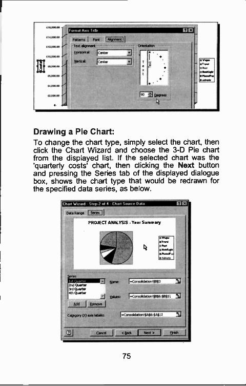
(16000 00

fit 000 00

413.000 00

,10.00000

I. 000 00

(5.00000

<61 000 00

000000

Format Axis Idle 12

Patterns Font LitText aagynent Onertatk:n

ttoroontal: ICertn

Ker tt

o Laxseas

Drawing a Pie Chart:To change the chart type, simply select the chart, thenclick the Chart Wizard and choose the 3-D Pie chartfrom the displayed list. If the selected chart was the'quarterly costs' chart, then clicking the Next buttonand pressing the Series tab of the displayed dialoguebox, shows the cl-art type that would be redrawn forthe specified data series, as below.

Chad Wezatd Step 2 et 4 - Chad Source Data 11

Data Range a-a7r1170 I

PROJECT ANALYSIS Year Summary

kConsoldaton,12$,

/dues: I-Cmsoidaturo$846

&dd I &moue I

CaLegory(X)Exts labeh: 1.,Consolelat0r0,SA$6 SAC:

Ce_Lical<e,d(J Next > Brach

75

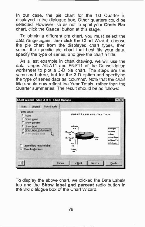
In our case, the pie chart for the 1st Quarter isdisplayed in the dialogue box. Other quarters could beselected. However, so as not to spoil your Costs Barchart, click the Cancel button at this stage.

To obtain a different pie chart, you must select thedata range again, then click the Chart Wizard, choosethe pie chart from the displayed chart types, thenselect the specific pie chart that best fits your data,specify the type of series, and give the chart a title.

As a last example in chart drawing, we will use thedata ranges A6:A11 and F6:F11 of the Consolidationworksheet to plot a 3-D pie chart. The steps are thesame as before, but for the 3-D option and specifyingthe type of series data as 'columns'. Note t'iat the charttitle should now reflect the Year Totals, rather than theQuarter summaries. The result should be as follows:

Chad Wizard - Step 3 id 4 - Chad Options

Tides I Legend Data Labels

i Date labelsC NQpe

Show tamer show Lemont

r Show label

(.7 IShow kibeiP_percentr -7-1717 _

r Legend I5,ey next to labelShow leader Ines

PROJECT ANALYSIS - Yea, Totals

Advertc20%

Phoneff at5%

IleatPlrq2%

Rest4%

9%

60%

Wars I ravela Rem

0 Neat/Light

41011.66efFsx

a Adverts

Cancel < tack I Next > I Ejntsh

To display the above chart, we clicked the Data Labelstab and the Show label and percent radio button inthe 3rd dialogue box of the Chart Wizard.

76

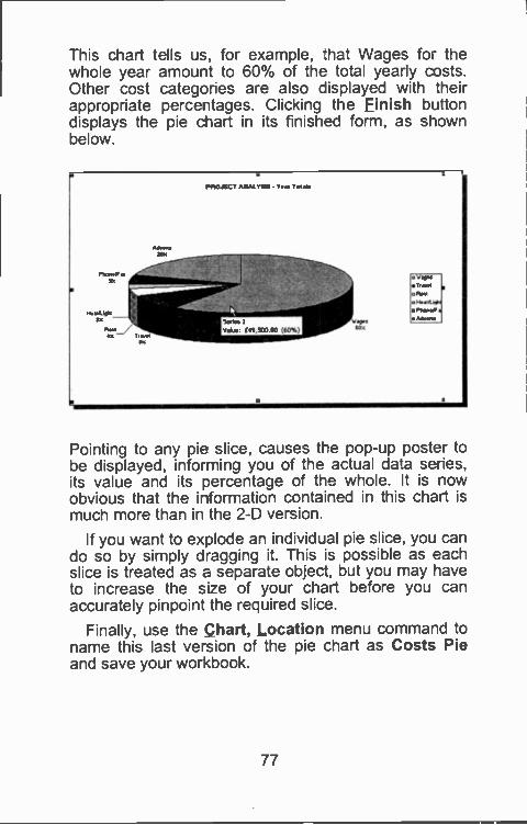
This chart tells us, for example, that Wages for thewhole year amount to 60% of the total yearly costs.Other cost categories are also displayed with theirappropriate percentages. Clicking the Finish buttondisplays the pie chart in its finished form, as shownbelow.

Pointing to any pie slice, causes the pop-up poster tobe displayed, informing you of the actual data series,its value and its percentage of the whole. It is nowobvious that the information contained in this chart ismuch more than in the 2-D version.

If you want to explode an individual pie slice, you cando so by simply dragging it. This is possible as eachslice is treated as a separate object, but you may haveto increase the size of your chart before you canaccurately pinpoint the required slice.

Finally, use the Chart, Location menu command toname this last version of the pie chart as Costs Pieand save your workbook.

77

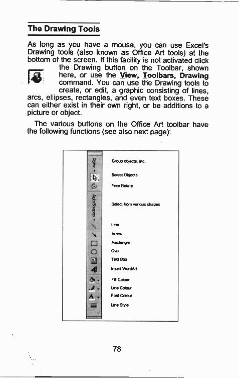
The Drawing Tools

As long as you have a mouse, you can use Excel'sDrawing tools (also known as Office Art tools) at thebottom of the screen. If this facility is not activated click

the Drawing button on the Toolbar, shownhere, or use the View, Toolbars, Drawingcommand. You can use the Drawing tools tocreate, or edit, a graphic consisting of lines,

arcs, ellipses, rectangles, and even text boxes. Thesecan either exist in their own right, or be additions to apicture or object.

The various buttons on the Office Art toolbar havethe following functions (see also next page):

O

4

A

Group objects. etc.

Select Objects

Free Rotate

Select from various shapes

Line

Arrow

Rectangle

Oval

Text Box

Insert WordArt

Fill Colour

Line Colour

Font Colour

Line Style

78

Office Art:Office Art is the new drawing tool shared by all Cffice97 applications and gives Excel 97 a superior graphicscapability. New or enhanced features are:

AutoShapes - the additional AutoShape categories,such as connectors, block arrows, flowchart symbols,stars and banners, callouts, and action buttons makedrawing diagrams much easier.

Bezier curves - used to easily create exact curveswith pin -point precision.

3-D effects - allow you to transform 2-D shapes intorealistic 3-D objects with new 3-D effects, such aschanging the lighting perspective of a 3-D object.

Perspective shadows - allow you to select from awide range of shadows with perspective, and you canadjust the depth and angle of each shadow to makepictures more realistic.

Connectors - used to create diagrams and flowct-artswith new straight, angled, and curved connectorsbetween the shapes; when shapes are moved, theconnectors remain attached and automaticallyreposition themselves.

Arrowhead styles - allow you to change the width andheight of arrowheads for maximum effect.

Object alignment - allows you to distribute and spaceobjects evenly, both horizontally and vertically.

Precise line -width control - allows you increasedcontrol over the width of lines by selecting presetoptions or customised line widths.

Image editing - lets you easily adjust the brightness orcontrast of a picture.

Transparent background - allows you to inse-t abitmap on your slides or Web pages so as to appear tobe part of the design by turning background coloursinto transparent areas.

79

Creating a Drawing:The effects of the drawing tools can be superimposedeither on the spreadsheet area or on top of a chart.The result is that you can annotate Excel 97worksheets or charts to your total satisfaction.

To create an object, click on the required Drawingbutton, such as the Oval or Rectangle, position themouse pointer where you want to create the object onthe screen, and then drag the mouse to draw theobject. Hold the <Shift> key while you drag the mouseto create a perfect circle or square. If you do not hold<Shift>, Office Art creates an oval or a rectangle.

You can use the AutoShapes button to select from avariety of pre -drawn Lines, Basic Shapes, etc. Firstclick on the desired line or shape, then position themouse pointer where you want to create the object onthe screen and click the left mouse buttcn to fix it onthat position.

Editing a Chart:To select a chart, click on it. Excel displays blackhandles around the selected chart. You can:

(a) Move an object, or multiple objects, within adraw area of a chart by selecting them and draggingto the desired position. To copy an object, click atthe object, then use the Edit, Copy / Edit, Pastecommands. (b) Size an object by positioning themouse pointer on a black handle and then draggingthe handle until the object is the desired shape andsize. (c) Delete an object by selecting it andpressing the <Del> key. To delete a drawing, holdthe <Shift> key down and click each object in turnthat makes up the drawing, unless they are groupedor framed, then press <Del>.

Do try out some of these commands using the Project9 Excel file, but do not save the results of yourexperimentation under the same file name.

80

5. THE EXCEL DATABASE

An Excel database table is a worksheet range whichcontains related information, such as 'Customer'sNames', 'Consultarcy Details', 'Invoice No.', etc. Aphone book is a simple database table, stored onpaper. In Excel eaci record is entered as a worksheetrow, with the fields of each -ecord occupyingcorresponding columns.

A database table is a collection of data that exists,and is organised around a specific theme orrequirement. It is used for storing information so that itis quickly accessible. To make accessing the Cataeasier, each row (or record), of data within a databasetable is structured ir the same fashicn, i.e. each recordwill have the same r umber of columns (or fields).

We define a database and its various elements asfollows:

Database table A collection of related dataorganised in rows and co umns ina worksheet file. A worksheet filecan contain many differentdatabase tables.

Record A row of information relating to asingle entry and comprising oneor more fields.

Field A single column of information ofthe same type, such as people'snames.

In Excel 97, a database table can contain a maximumof 256 fields and 65,536 records. Furthermore, you canhave up to 32,000 characters in a cell, increased froma previous limit of 256 in earlier versions of thepackage.

81

Creating a Database

In order to investigate the various database functions,such as sorting, searching, etc., we first reed to set upa database table in the form shown on the next page.

Note that in creating a database table, the followingrules must be observed:

1. The top row of the database table must containthe field labels, one per column, which identifythe fields in the database table. The second andsubsequent rows of such a database table mustcontain records; no blank rows should beinserted between the field labels and therecords.

2. Field labels must be unique within a givendatabase table.

3. Entries under each field must be of the sametype.

4. The size of a database table must be limitedwithin the design criteria of the package (256fields and 65,536 records for Excel 97).

We assume that the 'Invoice Analysis' of AdeptConsultants is designed and set out as shown belowwith the listed field titles and field widths.

Column Title Width TypeA NAME 21 General or TextB DETAILS 20 General or TextC No. 6 Number, 0 decimalsD ISSUED 9 Custom, dd/mm/yyE PAID? 7 General or TextF VALUE 8 Currency, 2 decimals

These widths were chosen so that the whole worksheetcould be seen on the screen at once.

82

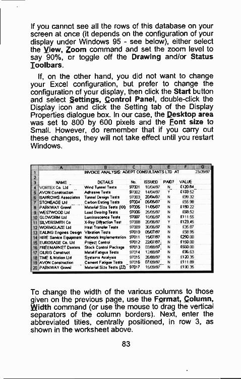
If you cannot see all the rows of this database on .jourscreen at once (it depends on the configuration of .,/ourdisplay under Windows 95 - see below), either selectthe View, Zoom command and set the zoom level tosay 90%, or toggle off the Drawing and/or StatusToolbars.

If, on the other hand, you did not want to changeyour Excel configuration, but prefer to change theconfiguration of your display, then click the Start bLttonand select Settings, Control Panel, double-click theDisplay icon and click the Setting tab of the DisplayProperties dialogue box. In our case, the Desktop areawas set to 800 by 600 pixels and the Font size toSmall. However, do remember that if you carry outthese changes, they will not take effect until you restartWindows.

2

C

INVOICE ANALYSIS ADEPT CONSULTANTS

U TA.ILS No

0 I E F 02309/97

VALUENAME

LTD AT

ISSUED PAID?

4 VORTEX Co Lid Wind Tumel Tests 971331 10/34/97 N f 120 84

AVON Construction Adhesive Tests 97002 110497 V £133 52

ELARROBARROWS Associates Tunnel Design Tests 97003 211134/97 N E39 32

7 STONEAGE Ltd Carbon Dating Tests 9703/ 0546/97 N £5598

8 PARKWAY Gravel Matenal Size Tests (>01) 97005 11135/97 N £130 22

9 VVESTWOOD Ltd Load Beaing Tests 97036 25/3567 N 03 5210 GLOWORM lid Luminescence Tests 971:07 113/36/97 N E111 55

11 SILVERSMITH Co X.Ray Diffraction Test 97008 20/C6/37 Y £12315

IP WORMGLAZE Ltd Heat Transfer Tests 97009 310667 N £35 87

13 EALING Engines Design Vibration Tests 97010 05/3767 N iE15957

14 HIRE Service Equipment Network Implementation 97011 15/37/97 N E290 CO

15 EUROBASE Co Ltd Project Control 97012 22437/97 N £1500016_,- FREEMARKET Dealers Stock Control Package 97013 0368.67 N £55000

11 OILRIG Construct Metal Fat gue Tests 97011 1246/97 N £36 63

la TIME & Motion Ltd Systems Analysis 97015 26/013137 N E 1 20 35

19 AVON Construction Cemert Fatigue Tests 97016 0703/97 N E111 E9

20_ PARKWAY Gravel Material Tire Tests (11) 97017 15/09/97 N £130 35

To change the width of the various columns to thosegiven on the previous page, use the Format, Column,Width command (or use the mouse to drag the vericalseparators of the column borders). Next, enter theabbreviated titles, centrally positioned, in row 3, asshown in the worksheet above.

83

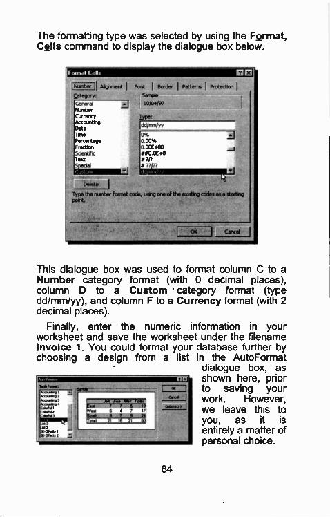
The formatting type was selected by using the Format,Cells command to display the dialogue box below.

From,. Cells 1112

Cf:.11iiii.21 Alignment I Font I Border I Patterns I Protectlen

category:GeneralNumberCurrencyAccountingDateTimePercentageFractionScientificTextS... ial

SeeTPle

10104/97

Type:

IdclinTNYY

0%0.00%0.00E+00**0.0E+0*?/?:n 7

_J

Ze3r-Ae

Type the number format code, using one of the cough; codes es a stertngpont.

OK Cancel

This dialogue box was used to format column C to aNumber category format (with 0 decimal places),column D to a Custom category format (typedd/mm/yy), and column F to a Currency format (with 2decimal places).

Finally, enter the numeric informat on in yourworksheet and save the worksheet under the filenameInvoice 1. You could format your database further bychoosing a design from a list in the AutoFormat

dialogue box, asshown here, priorto saving yourwork. However,we leave this toyou, as it isentirely a matter ofpersonal choice.

In Fob Mir Tao 1

7 6 1A6

1

8 7 9 KI2 16 21 60,

84

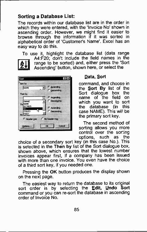
Sorting a Database List:The records within our database list are in the order inwhich they were entered, with the 'Invoice No' shows inascending order. However, we might find it easie- tobrowse through the information if it was sortec inalphabetical order of 'Customer's Name'. Excel has aneasy way to do this.

To use it, highlight the database list (data rangeA4:F20; don': include the f eld names in therange to be sorted) and, either press the 'SortAscending' button, shown here, or select the

Data, Sort

command, and choose inthe Sort By list of theSort dialogue box thename of the field onwhich you want to sortthe database (in thiscase NAME). Th s wil bethe primary sort key.

The second method ofsorting allows you morecontrol over the sor.ingoptions, such as the

choice of a secondary sort key (in this case No.). Thisis selected in the Then by list of the Sort dialogue box,shown above, whici ensures that the lowest numberinvoices appear first, if a company has been issuedwith more than one invoice. You even have the choiceof a third sort key, if you needed one

Pressing the OK Dutton produces the display shownon the next page.

The easiest way to return the database to its originalsort order is by selecting the Edit, undo Sortcommand or you cal re -sort the database in ascendingorder of Invoice No.

85

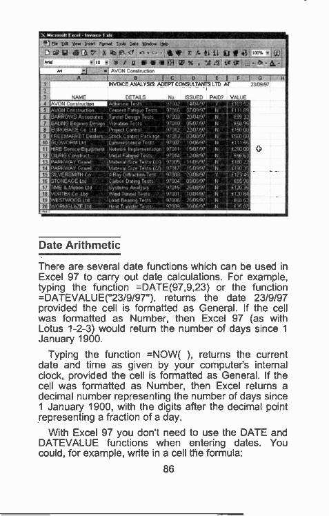
X MociotoIt Excel lonaIce I d.

OS ten Yoe Format Doi, Lift a ginclow twp

Df3IR X

Ana IC nrullEille Mtn; a x.4.1 a Or LL -4 -Al AVON Construction

A MENIIMEN11111111111111131111111111C11111 IMAM G

2

3

4

NAME

INVOICE ANALYSIS ADEPT CONSULTANTS LTD AT

DETAILS No. ISSUED PAID? VALUE

2309/97

VON Constiuction

ROWS Associates Tunnel Design Tr .t .G Engines Design : \Ablation Tests

UROBASE Co Ltd ...jp.ncitact ContioiREEMARlitT Dealers. IStock Control F i- k :la

X43337010.'47112.

i7313._

2:10:, .

05/1.1,7)

2207/97030-3/37

111 ;LON/ ORM Ltd '1..ummoscence TeSt" 17.xo 10,0E097 IIal HIRE Semce Equipment Nel-;1-1:, i'/...p-i.mentatioi. 37011. 160751.7 N

In ALRIG Construct. Metal Fallsoot Tests .i7014 12E097 Nill ..-JAMWAY Gravel 1MaterialSize Teuio f,.. ? 971.05. 110V/7. N ft,Elpi . 'AMWAY Gravel

-,Lvezwer, C ,1.Mate9.1 SizTests (l.') '700,

170011601/1720.081/47

N

Y-LiGy Dilbaction,e.:tIn 3TONEAGE Lid ,:ailion Dating:tests 170104.. 0505/97. N

lariME &Molion Lt. Systems Analysis. '.47015: 2608/97 NET ,, ,RIFT Cs I Id '/Vind Tunnel Tests '17001 10E34)97 N

Ila -.ETry m -r -f, L .6 Ln ad Beating Tests 97036 25k1S9.7 N

HAI1Trans(pr TelE1 VEEP 7,A.:kr.,17 N

H

Date Arithmetic

There are several date functions which can be used inExcel 97 to carry out date calculations. For example,typing the function =DATE(97,9,23) or the function=DATEVALUE("23/9/97"), returns the date 23/9/97provided the cell is formatted as General. If the cellwas formatted as Number, then Excel 97 (as withLotus 1-2-3) would return the number of days since 1January 1900.

Typing the function =NOW( ), returns the currentdate and time as given by your computer's internalclock, provided the cell is formatted as General. If thecell was formatted as Number, then Excel returns adecimal number representing the number of days since1 January 1900, with the digits after the decimal pointrepresenting a fraction of a day.

With Excel 97 you don't need to use the DATE andDATEVALUE functions when entering dates. Youcould, for example, write in a cell the formula:

86

=NOW() -D4

which allows Excel 97 to calculate the difference indays between now and the mentioned date.

We could use this formula to work out the number ofoverdue days of the unpaid invoices in our example, bytyping it in cell G4. However, if you want to comparethe numbers you get with those displayed in his book,use instead the following formula:

=$G$1 -D4

where $G$1 causes an 'absolute' reference to bemade to the conterts of cell G1. If the record in rcw 4of the worksheet refers to the data of VORTEX Co.Ltd., then the result should be 166 days, provided youare doing this after midday, otherwise it will be 165.

However, before we proceed to copy the atoveformula to the rest of the G column of the database list,we should take nto consideration the fact that,normally, such information is not necessary if aninvoice has been paid. Therefore, we need to edit theabove formula in such a way as to make the resultconditional to non-payment of the issued invoice.

The IF Function

The IF function allows comparison between two valueswith the use of special 'logical' operators. The logicaloperators we can use are listed below.

Logical operatorsEqual toLess thanGreater than

<= Less than or Equal to>= Greater than or Equal to<> Not Equal to

The general format of the IF function is as follows:

87

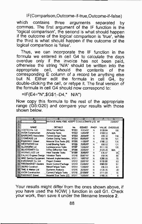
IF(Comparison,Outcome-if-true,Outcome-if-false)

which contains three arguments separated bycommas. The first argument of the IF function is the'logical comparison', the second is what should happenif the outcome of the logical comparison is 'true', whilethe third is what should happen if the outcome of thelogical comparison is 'false'.

Thus, we can incorporate the IF function in theformula we entered in cell G4 to calculate the daysoverdue only if the invoice has not been paid,otherwise the string 'N/A' should be written into theappropriate cell, should the contents of thecorresponding E column of a record be anything elsebut N. Either edit the formula in cell G4, bydouble-clicking the cell, or retype it. The final version ofthe formula in cell G4 should now correspond to:

=1F(E4="N",$G$1-D4," N/A")

Now copy this formula to the rest of the appropriaterange (G5:G20) and compare your results with those

A B C D E

CONSULTANTS LTD AT "i3)09971 1 INVOICE ,ANAI YSIS ADEPT2

3 NAME DETAILS No ISSUED PAD, VALVE OVERDUE4 VORTEX Co Ud Wind Tunnel Tests 9/0131 10/0097 N £120.84 1665 AVON Construction Adhesrve Tests 97002 14,04)97 Y £103 52 N/A6 -BARROWS Associates Tunnel Design Tests 970133 20/0097 N f99 32 156

STONEAGE Ud Carbon Dating Tests 971304 093597 N £55 98 141

PARKWAY Gravel Matenal Size Tests c2 970% 1135/97 N 6180 22 1359' MESTWOOD Ud--'110 GLOWORM Ud

Load Beanng TestsLuminescence Tests

9700697007

2505/971006/97

N

N

£68 52£111 55

121

10511 ;SILVERSMITH Co X -Ray Diffraction Test 97008 2036/97 Y £123 45 N/A12 WORMGLAZE Ud Heal Transfer Tests 97003 3306197 N £3581 8513 l.ALING Engines Design Vibration Tests 97010 05/37/37 N £58 95 B314 HIRE Serino. Equipment Network Implementation 97011 15.0797 N £290 0113 7015 F-VROBASE Co Ltd Project Control 97012 2237/97 N £15000 6316 F REEMARKET Dealers Stock Control Package 97013 01138/97 N f56000 51

17 ()TRIG Construct Metal Fatigue Tests 97014 12/3197 N E% 63 4218 TIME 8. Motion Ltd Systems Analysis 97015 26/01197 N £12.35 2819 AVON Construction Cement Fatigue Tests 97016 0708/97 N f111 .69 16

20 PARKWAY Gravel Matenal Size Tests (ZZ) 97017 150997 N 6190 35 8

Your results might differ from the ones shown above, ifyou have used the NOW( ) function in cell G1. Checkyour work, then save it under the filename Invoice 2.

88

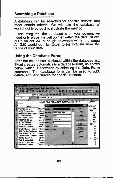
Searching a Database

A database can be searched for specific records thatmeet certain criteria. We will use the database ofworksheet Invoice 2 to illustrate the method.

Assuming that the database is on your screen, weneed only place the cell pointer within the data list (weput it on cell A4, although anywhere within the rangeA4:G20 would do), for Excel to instinctively know therange of your data.

Using the Database Form:After the cell pointer is placed within the database list,Excel creates automatically a database form, as shownbelow, which is accessed by selecting the Data, Formcommand. The database form car be used to add,delete, edit, and search for specific records.

\ e

JIVE. gait VW kind Pormul.ads _w:>eeow tWP

!ID Cie 41M -0!:i Rift Cr - - ft 1- Gil a till IC°.4jAd 10 / 4O_FHISP % 4421P1--

A4

1_

23-1 NAME

Co Ltd3

INVOICE ANALYSIS ADEPT CONSULTAYTS LTD AT

frAnd T' Nem: f11111111111111.14 RTEX Co Lld5 AVON Construction Adhesk

.61 BARROWS Associates Tunnel OC ARS: lverd Trnn Teas

7,STONEAGE Ud Carbon Ni- 19700

PARKWAY Gravel Matena9 WESTWOOD Ud Load BLss-itm 1,0 /1917

to GLOVVORM Ltd Lumina ply, lx11 SILVERSMITH Co X -Ray I

12 WORMGLAZE Ltd Heat Tr VAILEt 1,2'0 84

13 EALING Engines Design Vtbratio

14 HIRE Service Equipment Nations/I

16 EUROBASE CO Ud Project16 FREEMARKET Dealers Stock17 OILRIG Construct Metal F

le TIME & Motion Ud Systerr19 AVON Construction Cement

20 PARKWAY Gravel Maters

21

71459/97

RDIJE

1 kN/A

1;6I11

1 15

1 ?I

1 15

N/A16

10

*0

:3

.2

6

89

Note that the field names at the top row of thedatabase appear on the left side of the form. On thetop right corner of the form (above the New button) theentry '1 of 17' is displayed to indicate that this is thefirst of 17 records.

Most of the field names within the database formhave one letter underlined, which can be used toaccess the corresponding box in the middle of the formin which the value of each field of the particular recordis shown. To select fields or buttons, press the <Alt>key plus the underlined letter on field text or button, orpoint and click with the mouse. To move the highlighterforward through fields and buttons press the <Tab>key, while to move backwards, press <Shi:t+Tab>.

With the help of the database form, adding newrecords is made easy. On pressing the New button, anempty form is displayed for you to fill in. Editing adisplayed record is even easier; that is why theRestore button is included. The functions of the formbuttons are as follows:

Button FunctionNew Clears the field entries in the displayed

form so that new information can beadded. Pressing New again, adds thedata just typed as a new record in thedatabase.

Delete Deletes the displayed record and shiftsthe remaining records one up the list. Adeleted record cannot be restored. Ifyou delete a record accidentally,re -open the database file without savingthe changes.

Restore Restores edited fields in the displayedrecord, removing the changes justmade. Entries must be restored beforepressing <Enter> to scroll to anotherrecord, or clicking the Close button.

90

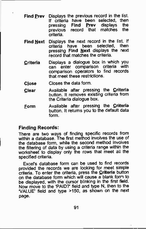
Find Prey Displays the previous record in the list.If criteria have been selected, Thenpressing Find Prey displays theprevicus record that matches thecriteria.

Find Next Displays the next record in the list. Ifcriteria have been selected, thenpressing Find Next displays the nextrecord that matches the criteria.

Criteria Displays a dialogue box in which youcan enter comparison criteria withcomparison operators to find recordsthat rreet these restrictions.

Close Closes the data form

Clear Available after pressing the Criteriabutton. It removes existing criteria fromthe Criteria dialogue box.

Form Available after pressing the Criteriabutton. It returns you to the default dataform.

Finding Records:There are two ways of finding specific records fromwithin a database. The first method involves the use ofthe database form, while the second method invo vesthe filtering of data by using a criteria range within theworksheet to display only the rows that meet all thespecified criteria.

Excel's database form can be used to find recordsprovided the records we are looking for meet simplecriteria. To enter the criteria, press the Criteria buttonon the database form which will cause a blank form tobe displayed, with the cursor blinking in the first field.Now move to the 'PAID?' field and type N, then to the'VALUE' field and type >150, as shown on the nextpage.

91

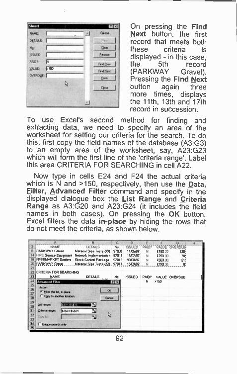
Sheet* 11©

DLTAJLS

N0

ISSUED

ENV

yituE.

OVERDUE

On pressing the FindJ Caen. Next button, the first

record that meets bothCJe. these criteria is

displayed - in this case,the 5th record(PARKWAY Gravel).Pressing the Find Nextbutton again threemore times, displaysthe 11th, 13th and 17threcord in succession.

To use Excel's second method for finding andextracting data, we need to specify an area of theworksheet for setting our criteria for the search. To dothis, first copy the field names of the database (A3:G3)to an empty area of the worksheet, say, A23:G23which will form the first line of the 'criteria range'. Labelthis area CRITERIA FOR SEARCHING in cell A22.

Now type in cells E24 and F24 the actual criteriawhich is N and >150, respectively, then use the Data,Filter, Advanced Filter command and specify in thedisplayed dialogue box the List Range and CriteriaRange as A3:G20 and A23:G24 (it includes the fieldnames in both cases). On pressing the OK button,Excel filters the data in -place by hiding the rows thatdo not meet the criteria, as shown below.

fientcoe

Feld Ern

Fnd5na

S1_2_14

A B3 i NAME DETAILS 1 NoifilRARKWAY Gravel Matenal Size Tests pal 970135--414 rHIRE Sonic. Equipment Network Implement allon 97011IS f REEMARKET Dealers Stock Control Package 970131:111iPARKWAY Gravel Matenal Size Tests WI 97017

na CRITERIA FOR SEARCHINGNAMI

24

25

2627

26

293031 Crtects rage $4$24

32

33

Unctur rerrack cveY35

Advancncl igen

DETAILS No

/Ann FT-A16. titer the kt,r" qv, to VIShilt Malt

lot ...a. 11901 al

ISSUED PAID? VALUE OVERDUE.110597 N 0183 22 135

150707 N 029000 70030807 N 1560 00 51

1509/97 N 0190 35 8

ISSUED PAID? VALUE OVERDUEN .150

92

Do not specify an empty line as part of the criterionrange, as this has the effect of searching the databasefor all records. The criteria must be entered in thesecond and subsequent rows of the criterion range,with each entered below the copy of the appropriatefield name. A label (text) or a value may be enteredexactly as it appears in the database.

In the case of searching a database for label (text),such as under the fields 'NAME' and 'DETAILS' in ourexample, you can use the two special characters and* (known as 'wildcard characters') to match any singlecharacter of a label or all characters to the end of thelabel.

To search a database for values, either enter thevalue as the exact criterion or use a simple numericcomparison, such as >90, in which the logicaloperators (<, <=, >, >=, <>) can be used. The logicalformula generates a value of 1 if the condition is TRUEor a value of 0 if the condition is FALSE.

Several criteria can be entered, either in the samerow, if you want Excel to search for records that matchevery criterion (i.e. criteria entered are linked with thelogical AND), or one per row, if you want Exce! tosearch records that satisfy any o' the criteria (i.e.criteria entered are linked with the logical OR).

As seen above, selecting the Filter the list, in -placeoption in the Advanced Filter dialogue box, causesExcel to hide the rows that do not meet the specifiedcriteria. To see the 'ull database list again, use theData, Filter, Show All command.

93

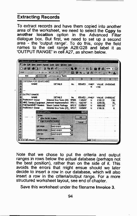
Extracting Records

To extract records and have them copied into anotherarea of the worksheet, we need to select the Copy toanother location option in the Advanced Filterdialogue box. But first, we need to set up a secondarea - the 'output range'. To do this, copy the fieldnames to the cell range A28:G28 and label it as'OUTPUT RANGE' in cell A27, as shown below.

\

fmdf

foyoK,

EM Edit VOW riot roma Lodi Clem *dew beb

A t 1111 I 4120-- -A

. to . N I u I:= ..7" OtcP% # MITEno j Luminescence Tests

A B .1 C 0 E FLOEM CRITERIA FOR SEARCHING23 NAME DETAILS No ISSUED PAID, VALUE OVERDUE24 N .150251

26,77:OUTPUT RANGE28 NAME DETAILS No ISSUED PAIDT VALUE OVERDUE29 PARKWAY Gravel Material Size Tests 001) 970I35 11,135/37 N MO 22 1353) HIRE Seneca Equipment Network Implementation 97011 15/0797 N E29000 7031 FREEMARKET Dealers Stock Control Package 97013 03.4:18/97 N £560 00 5132 PARKWAY Gravel Matenal Size Tests (ZZ) 97017 15A)9/37 N £190 35 833

Advanced Flret34361

rd38

Action

r Liter the 1st, Veciece C. If. to locomen!

- 14Ust ramp: liat3 5C42039.

413 Oterle rang. ISM23.8G62441

42 Copy spa f1A$28,1G$49

43 r Leccves wet* 1.1

Note that we chose to put the criteria and outputranges in rows below the actual database (perhaps notthe best position), rather than on the side of it. Thisavoids the errors that might ensue should we laterdecide to insert a row in our database, which will alsoinsert a row in the criteria/output range. For a morestructured worksheet layout, see end of chapter.

Save this worksheet under the filename Invoice 3.

94

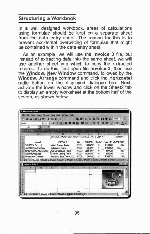
Structuring a Wcrkbook

In a well designed workbook, areas of calculationsusing formulae should be kept on a separate sheetfrom the data entry sheet. The reason for this is toprevent accidental overwriting of formulae that mightbe contained within the data entry sheet.

As an example, we will use the Invoice 3 file, butinstead of extracting data into the same sheet, we willuse another sheet into which to copy the extractedrecords. To do this. first open file Invoice 3, then usethe Window, New Window command, followed by theWindow, Arrange command and click the Horizontalradio button on the displayed dialogue box. Next,activate the lower window and click on the Sheet2 tabto display an empty worksheet at the bottom half of thescreen, as shown below.

6 ea tars irrmrf PS1.44 Loa. Ws WM.* Belo

Daulea7lx Rba,--f - r 44111 1114 c"x tZ

10 sin EiragICVx,IfIVYWO 3. x14.2

A ' C 0 E 1

INVOICE ARAL YSIS ADEPT CONSULTAN-S ( TO ATo

73,09,97

2

3 NAME CETAILS No ISSUED PAID? VALUE OVERDUE4 'VORTEX Co Ltd Wind Tune Tests 97001 1094137 N f 120 91 166

5 ,AVON Construction Adhesive Tests 971322 1413497 Y £10352 N/A

6 BARROWS Associates Tunnel Design Tests 97003 200497 N £99 32 156

7 STONEAGE Ltd Carbon C *beg Tests 97004 0533597 N £55 98 141

B 'PARKWAY Gravel Matenal 310 Tests (XX) 971335 1005.97 N f 1E13 72 135

14 ' 4 k 'aiNtheetliPeat2 Igheat3_73etS_ISheeek_Teagt7_21114441jA1411011hial

Invoice At I emA

2

3

567

g"410 9wmulsheer ilhildaVialEalL4LstisE6_4111_

B C F

95

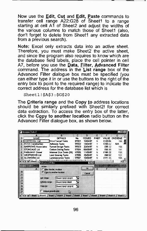
Now use the Edit, Cut and Edit, Paste commands totransfer cell range A22:G28 of Sheetl to a rangestarting at cell Al of Sheet2 and adjust the widths ofthe various columns to match those of Sheetl (also,don't forget to delete from Sheetl any extracted datafrom a previous search).

Note: Excel only extracts data into an active sheet.Therefore, you must make Sheet2 the active sheet,and since the program also requires to know which arethe database field labels, place the cell pointer in cellA7, before you use the Data, Filter, Advanced Filtercommand. The address in the List range box of theAdvanced Filter dialogue box must be specified (youcan either type it in or use the buttons to the right of theentry box to point to the required range) to indicate thecorrect address for the database list which is

Sheetl!$A$3:$G$20

The Criteria range and the Copy to address locationsshould be similarly prefixed with Sheet2! for correctdata extraction. To access the entry box of the latter,click the Copy to another location radio button on theAdvanced Filter dialogue box, as shown below.

ifIVOICII 3 oh 2 FIREA B' t C D E F G -

3 NAME DETAILS No ISSUED PAID? VALUE OVERDUE -4 !VORTEX Co Ud IMind Tunnel Tests 97031 10434/97 N £12084 166

5 AVON Construction Adhesrve Tests 97002 14434/97 V £103 52 N/A6 BARROWS Associates Tunnel Design Tests 971113 3343497 N E99 32 156

7 STONEAGE Ud Carbon Dating Tests 97034 05/05/97 N 655 913 141

8 PARKWAY Gravel Material Size Tests (G 97005 11/05/97 N 6180 22 135

9 WESTWOOD Ltd Load Bearing Tests 971E06 2505437 N £66 52 121

10 GLOWORM Ltd Luminescence Tests 971337 10436/97 N--.--/$$ .1

9Te_Ttit.Advuncudhilu/

gator) --- --A r Eit. the Itit, bows

20 r: cal.>, to another WW121

!sheen 4A$3 $C$2023

24crteriard.P: ISheet2.0$24GS3

25 COPY LP: ISheet2.$O$7$G$241

2627 r unique ("twitch*

yr4 it MA ),51leet 2 X 511.4413hestliThoptlf X %seta Lhiptliguiltt Xfrest9 plastic

EZE1

ok I

cad j

6111 55 135

!Jr;

E

_11

,.1

96

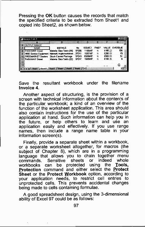
Pressing the OK button causes the records that matchthe specified criteria to be extracted from Sreetl andcopied into Sheet2, as shown below.

ji !name 3 ids 1

A

PIRO

6 OUTPUT RANGE71 NAME

1DETAILS No ISSUE 3 PAID? VALUE OVERDJE

8 PARKWAY Gravel Matena Sme Tests (V) 97005 11D5k37 N £1130 Z2 135

9 HIRE Service Equipment Networi Implementation 97011 15,0797 N £29003 70

10 FREEMARKET Dealers Stock ( on rol Package 97013 03/3897 N E560 0) 51

11 PARKWAY Gravel Matena Sits Tests (22) 97017 15,0997 N £190 3 8

12

13 0 alTi4 p :m \ 916011 )0/wet? X Sheei iShesti ShestS Shoet6 / I 4 I ,r,,

Save the resultant workbook under the filenameInvoice 4.

Another aspect of structuring, is the provision of ascreen with technical information about the conten:s ofthe particular workbook; a kind of an overview of thefunction of the worksheet application. This area shouldalso contain instruct ons for the use of the oarticularapplication at hand. Such information can help you inthe future, or help others to learn and use anapplication easily and effectively. If you use rangenames, then include a range name table in yourinformation screen(s).

Finally, provide a separate sheet within a workbook,or a separate worksheet altogether, for macros (thesubject of Chapter 3), which are in a programminglanguage that allows you to chain together menucommands. Sens tive sheets or indeed wholeworkbooks can be protected using the Tools,Protection command and either select the ProtectSheet or the Protect Workbook option, according toyour application needs, to restrict cell entries tounprotected cells. This prevents accidental chargesbeing made to cells containing formulae.

A good spreadsheet design, usinc the 3 -dimensionalability of Excel 97 could be as follows:

97

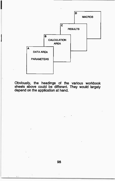
MACROS

RESULTS

CALCULATIONAREA

DATA AREA

PARAMETERS

Obviously, the headings of the various workbooksheets above could be different. They would largelydepend on the application at hand.

98

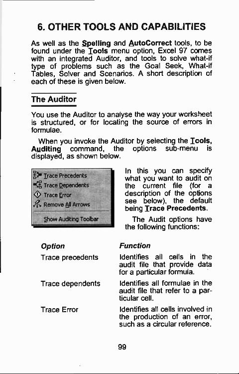
6. OTHER TOOLS AND CAPABILITIES

As well as the Spelling and AutoCorrect tools, to befound under the Tools menu option, Excel 97 comeswith an integrated Auditor, and tools to solve what -iftype of problems such as the Goal Seek, What -ifTables, Solver and Scenarios. A short description ofeach of these is given below.

The Auditor

You use the Auditor to analyse the way your worksheetis structured, or for locating the source of errors informulae.

When you invoke the Auditor by selecting the Tools,Auditing command, the optio'is sub -menu isdisplayed, as shown below.

1.)° Trace Precedents

-17, Trace

O' Trace Error

ev. Remove All Arrows

Show Auditing Toolbar

In this you can specifywhat you want to audit onthe current file (for adescription of the optionssee below), the defaultbeing Trace Precedents.

The Audit options havethe following functions:

Option Function

Trace precedents Identifies all cells in theaudit file that provide datafor a particular formula.

Trace dependents Identifies all formulae in theaudit file that refer to a par-ticular cell.

Trace Error Identifies all cells involved inthe production of an e-ror,such as a circular reference.

99

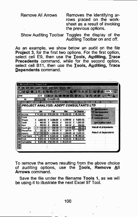
Jan Feb Mar 1st (loader

4 Income £ 14poo oo £1505050 E 16,003 00 £ 45030 CO

5 Costs6 Wages £ 200000 f 3,00050£ 4,05050 f 9 030 C13

7 Travel £ 400.00 £ 500.00 £ 600 00 f 1 503 50

8 Rent £ 300 00 f 300 00 £ 300 00 £ 900.00

9 Heat/Light10 Phone/Fax f 250 D3 £ 30800 £ 393 133 E 9013 00

11 Adverts;4,200

50

12 Total Costs £ 00 £ 5,500.00 £ 6,60000 E 16,330 00

13 Profit f 9,800 00 f 9,500 00 f 9,320 00 f 28,620 00

11 Cumulatme f 9,60000 619,330 00 £ 26,6205015_

J

Remove All Arrows Removes the identifying ar-rows placed o i the work-sheet as a result of invokingthe previous options.

Show Auditing Toolbar Toggles the display of theAuditing Toolba - on and off.

As an example, we show below an and t on the fileProject 3, for the first two options. For the first option,select cell E9, then use the Tools, Auditing, TracePrecedents command, while for the second option,select cell B11, then use the Tools, Auditing, TraceDependents command.

Mal 10

oik 0144914iif If*k

1 r.':,-1,11iAtt'r A II 1154i t00% -leveijor41:b2.,

F I ,,C1

PROJECT ANALYSIS: ADEPT CONSULTANTS LTDr Nee Precedents

Imre Damrdarts

O7..afmfr earsom &Arrows

So* Audetno Toolbar

Result of precedents

Result of dependents

To remove the arrows resulting from the above choiceof auditing options, use the Tools, Remove AllArrows command.

Save the file under the filename Tools 1, as we willbe using it to illustrate the next Excel 97 Tool.

100

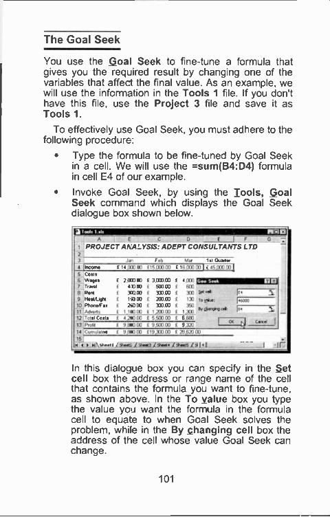
The Goal Seek

You use the goal Seek to fine-tune a formula thatgives you the required result by changing one of thevariables that affect the final value. As an example, wewill use the informat on in the Tools 1 file. If you don'thave this file, use the Project 3 file and save it asTools 1.

To effectively use Goal Seek, you must adhere to thefollowing procedure:

Type the formula to be fine-tuned by Goal Seekin a cell. We will use the =sum(B4:D4) formulain cell E4 of our example.

Invoke Goal Seek, by using the Tools, goalSeek command which displays the Goal Seekdialogue box shown below.

A

1 PROJECT AAAL.YSIS: ADEPT CONSULTANTS LTD2

3 Jan Feb Mar 1st QuarterIncome

5 Costs

f 14C00 00 £15 003 00 f 1600003

6_ Wages f 2=80 £ 30:003 £ 4.0007 Travel f C O00 500.00 f 6036 Reni f 300.00 f 300 00 f 330

9 Heal/light f 150 00 £ 200.00 £ 133

83_ Phone/Fax £ 2b030 £ 300.00 f 350

11 Adreds f 1,11013 f 1,20000 f 1,X012 Total Costs £ 4,29000 £ 5,50000 £ 6,6E10

13 Prole £ 9,880 00 £ 9,500.00 f 9,320

14 Cumulative I 9,E80 OD 119,300 00 f 20,62015.

Lao Seek

to

lot &mows.

Et

.6000

04

I 0

a

°few

00

-ThimMenet /shwa awn Imam Hisses 1)1 4L___ _J 4.7

In this dialogue box you can specify in the Setcell box the address or range name of the cellthat contains the formula you want to fine-tune,as shown above. In the To value box you typethe value you want the formula in the formulacell to equate to when Goal Seek solves theproblem, while in the By changing cell box theaddress of the cell whose value Goal Seek canchange.

101

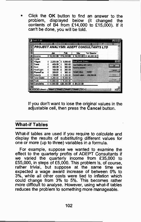
Click the OK button to find an answer to theproblem, displayed below (it changed thecontents of B4 from £14,000 to £15,000). If itcan't be done, you will be told.

2 l oots 1 olo

A 8 '1 C 1 0

1 PROJECT ANALYSIS: ADEPT CONSULTANTS LTD23

4

56

7

11

9

10

11

12

13

14

15 -

4 rImNsh-tirsiTst240..i.kol*,..o4/9e0e1511.1__ I sir

Jan Feb

Income f 15,030 CO 015,003 DO

CostsWages E 2,0013 00 I 3,000 OJ'ravelKO DO I 500 00Rent E 30000 £ 30013HeatilJgbt f 150.00 0 200Phone/Fan 25000 £ 30000Adverts £ 1,10000 1700133Total Costs f 420000 f 5,5000DProfit E 10 800 00 f 9,500 00Cumulat tee I 10 ,803 00 E20,310 00

Mar t lit (Duarte,

f 16,Om CO I f 46,000 001

Goo( Serb Stratus asGod Sedan; eat, Cal Li

loud a solutcn.

leb7M mime' 46000

Cigna ream: E46,CCO.00

f 29,620 CC

If you don't want to lose the original values in theadjustable cell, then press the Cancel button.

What -if Tables

What -if tables are used if you require to calculate anddisplay the results of substituting different values forone or more (up to three) variables in a formula.

For example, suppose we wanted to examine theeffect to the quarterly profits of ADEPT Consultants ifwe varied the quarterly income from £35,000 to£55,000, in steps of £5,000. This problem is, of course,rather trivial, but suppose at the sane time weexpected a wage award increase of between 0% to3%, while all other costs were tied to inflation whichcould change from 3% to 5%. This becomes rathermore difficult to analyse. However, using what -if tablesreduces the problem to something more manageable.

102

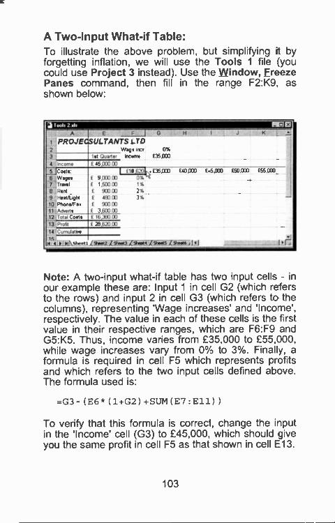
A Two -Input What -if Table:To illustrate the above problem, but simplifying it byforgetting inflation, we will use the Tools 1 file (youcould use Project 3 instead). Use the Window, FreezePanes command, then fill in the range F2:K9. asshown below:

Tech 2.x/le WI. ElA, E G r1 I J K L

1 PROJECSULTANTS &JD2 Wag, err 0%

3 lot Quarter Incemt E35,1:03

4 Income £ 45,000 00

5 [Costs 1 fie:04,e 05,000 £40,030 £4,000 00000 E55)106 E 9,00000 0104_Wages7 Travel £ 1,500 00 1%

0 Rent £ 90000 2%

9 Heat/Light £ 18000 3% -10 Phone/Fax £ 903 0011 Adverts £ 3,603 0012 Total Costs £ 16,3E0 03

13 Profit f 26,620 0014 Cumulative5

14 1 P M \ Sheet 1 /Sheet i Siisel Z5heast4 iSheetS / Sheet* , 1 1 I IA

Note: A two -input what -if table has two input cells - inour example these are: Input 1 in cell G2 (which refersto the rows) and input 2 in cell G3 (which refers to thecolumns), representing 'Wage increases' and 'Income',respectively. The value in each of these cells is the firstvalue in their respective ranges, which are F6:F9 andG5:K5. Thus, income varies from £35,000 to £55,000,while wage increases vary from 0°A to 3%. Finally, aformula is required in cell F5 which represents profitsand which refers to the two input cells defined above.The formula used is:

=G3- (E6* (1+G2) +SUM (E7 :Ell) )

To verify that this formula is correct, change the inputin the 'Income' cell (G3) to £45,000, which should giveyou the same profit in cell F5 as that shown in cell E13.

103

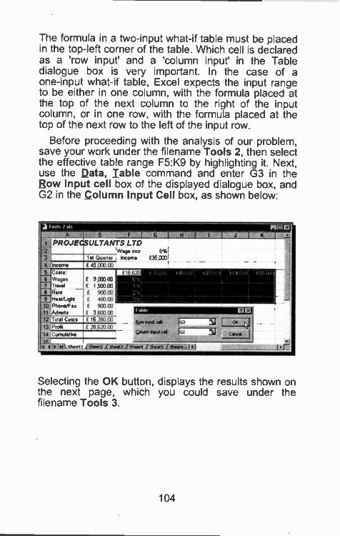
The formula in a two -input what -if table must be placedin the top -left corner of the table. Which cell is declaredas a 'row input' and a 'column input' in the Tabledialogue box is very important. In the case of aone -input what -if table, Excel expects the input rangeto be either in one column, with the formula placed atthe top of the next column to the right of the inputcolumn, or in one row, with the formula placed at thetop of the next row to the left of the input row.

Before proceeding with the analysis of our problem,save your work under the filename Tools 2, then selectthe effective table range F5:K9 by highlighting it. Next,use the Data, Table command and enter G3 in theRow Input cell box of the displayed dialogue box, andG2 in the Column Input Cell box, as shown below:

I

2

311

ool s I sis

A

PROJEE ;

wnoIIIIMIIIIIIII11111111111111111111EIRIMEINI

ULTANTS LTDWage 1ncr 0%

£35.0001st Quarter Income

Income f 15 000 00Costs £18 .20UUWagesTravel

£ 9 ,CO3 00

f 1.6130 03

LI101ift

11 'Adverts

Rent

HeatibgetPhone/Fax

£ 900 00f 180 00£ 900 00I 3 rrr 00 1.shin II©

12 Total Costs £ 16 380.00 Bps Inpit a& G313 !Profit f 28 620 00

Cumulated!102 3111

Owen igut al:

. sheet

Selecting the OK button, displays the results shown onthe next page, which you could save under thefilename Tools 3.

104

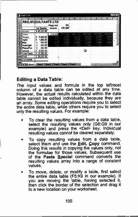
PROJECSULTANTS LTD23 1- 1st Quarter

4 Income £ 45,000 00

CostsWagesTravel

Rent

Heairbghl1911Phone/F as

1 Adverts12 Total Costs

tir_mi\s!,(ifigfighosis/shisbi /I 4

Editing a Data Table:The input values and formula in the top leftmostcolumn of a data table can be edited at any time.However, the actual -esults calculated within the catatable cannot be edited individually, because they arean array. Some editing operations require you to selectthe entire data table, while others require you toonly the resulting values. For example:

To clear the resulting values from a data to ple,select the resulting values only (G6:G9 in ourexample) and press the <Del> key. Indivicualresulting values cannot be cleared separately.

To copy resulting values from a data table,select them and use the Edit, Copy command.Doing this results in copying the values only, notthe formulae for those values. Subsequent useof the Paste special command converts theresulting values array into a range of constantvalues.

To move, delete, or modify a table, first seiectthe entire data table (F5:K9 in our example,. Ifyou are moving the table, having selected it,then click the border of the selection and drag itto a new location on your worksheet.

105

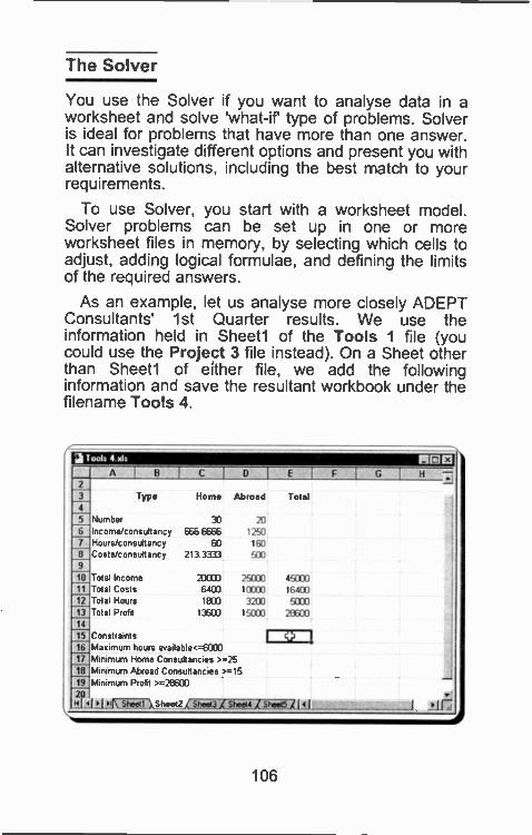
The Solver

You use the Solver if you want to analyse data in aworksheet and solve 'what -if type of problems. Solveris ideal for problems that have more than one answer.It can investigate different options and present you withalternative solutions, including the best match to yourrequirements.

To use Solver, you start with a worksheet model.Solver problems can be set up in cne or moreworksheet files in memory, by selecting which cells toadjust, adding logical formulae, and defining the limitsof the required answers.

As an example, let us analyse more closely ADEPTConsultants' 1st Quarter results. We use theinformation held in Sheet1 of the Tools 1 file (youcould use the Project 3 file instead). On a Sheet otherthan Sheet1 of either file, we add the followinginformation and save the resultant workbook under thefilename Tools 4.

a Tools 4 els PIWEIMI A o C o E F G

ElElIIIn

Type Home Abroad Total

Number 33 206 Income/consultancy 666 6666 1250Qri Hours/consultancy 60 160

Costs/consultancy 213 3333 5039

El Total Income 20003 25003 45000Eig Total Costs 6403 10000 16400Kggo

Total Hours 1803 3200 5000Total Profd 13603 1500T3 28E03

III15 Constraints

1 0 II0 Maximum hours available<=6000!IMI Minimum Home Consultancies >=25

Eiri Minimum Abroad Consultancies >=15Minimum Profit >=28603

2111

iiLlwpt_51.1,111 .I f7ksheet2j, _S_hgegi Sheet4 j_kheet5,1( IA

106

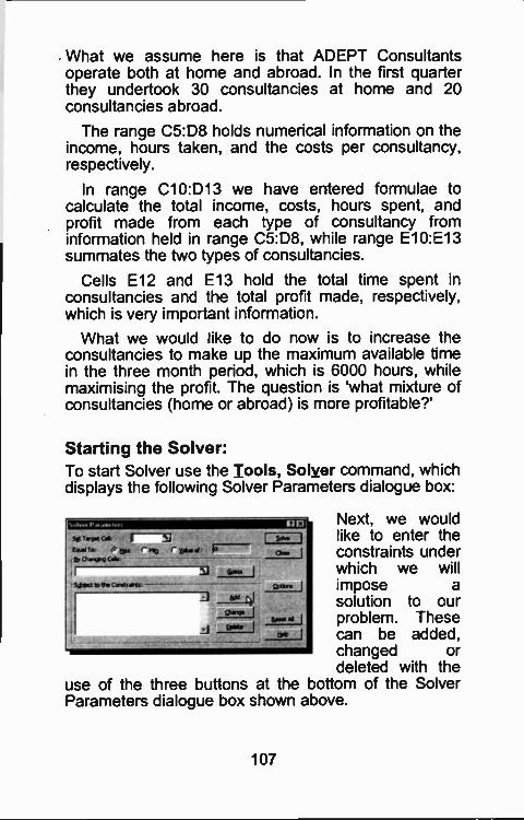
What we assume here is that ADEPT Consultantsoperate both at home and abroad. In the first quarterthey undertook 30 consultancies at home and 20consultancies abroad.

The range C5:D8 holds numerical information on theincome, hours taken, and the costs per consultancy,respectively.

In range C10:D13 we have entered formulae tocalculate the total income, costs, hours spent, andprofit made from each type of consultancy frominformation held in range C5:D8, while range E10:E13summates the two types of consultancies.

Cells E12 and E13 hold the total time spent inconsultancies and the total profit made, respectively,which is very important information.

What we would like to do now is to increase theconsultancies to make up the maximum available timein the three month period, which is 6000 hours, whilemaximising the profit. The question is 'what mixture ofconsultancies (home or abroad) is mare profitable?'

Starting the Solver:To start Solver use :he Tools, Solver command, whichdisplays the following Solver Parameters dialogue box:

ollyes Itm.movires

Sit two* Gtik

CoAti To:

ch,r9

fl_.. [

rra r a;

%OW to Vt. Co./ &CS: -

js

J P_ _1`

CP_

Next, we wouldlike to enter theconstraints underwhich we willimpose asolution to ourproblem. Thesecan be added,changed ordeleted with the

use of the three buttons at the bottom of the So verParameters dialogue box shown above.

107

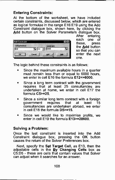
Entering Constraints:At the bottom of the worksheet, we have includedcertain constraints, discussed below, which are enteredas logical formulae in the range E16:E19 using the AddConstraint dialogue box, shown here, by clicking theAdd button on the Solver Parameters dialogue box.

Ater enteringeach one ofthese, pressthe Add button

160001

Caricel es t

otehratt hyr next

one.

Add Constiaint o©Cell Reference:

1E12

OK

constrant:

"2:1

The logic behind these constraints is as fo lows:

Since the maximum available hours in a quartermust remain less than or equal to 6000 hours,we enter in cell E16 the formula E12<=6000.

Since a long term contract with the governmentrequires that at least 25 consultancies areundertaken at home, we enter in cell E17 theformula C5>=25.

Since a similar long term contract with a foreigngovernment requires that at least 15consultancies are undertaken abroad, we enterin cell E18 the formula D5>=15.

Since we would like to maximise profits, weenter in cell E19 the formula E13>=28600.

Solving a Problem:Once the last constraint is inserted into the AddConstraint dialogue box, pressing the OK buttoncauses the return of the Solver Preferences box.

Next, specify the Set Target Cell, as E13, then theadjustable cells in the By Changing Cells box asC5:D5 - these are cells that contain values that Solvercan adjust when it searches for an answer.

108

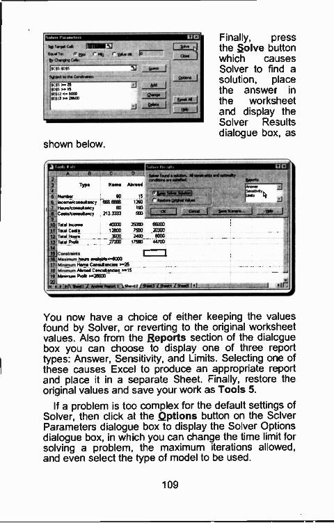
Solve, Pao...tett IUDsos ,arOsS

&pal Tor a tig.Itf ChrovI4-15 U4,

SSIDIKS to tha Combats

SCi5SCSi2raralaSt SI

.11

J - eraI

shown below.

'Typ Honi Abtod

Finally, pressthe solve buttonwhich causesSolver to find asolution, placethe answer inthe worksheetand display theSolver Resultsdialogue box, as

War laud Wrt. i en* efts ird newly*nifty en tashoil yyets

we s4.

6 Number 60 5 WEESSE9r NamInc orneic onsuanc y 656 6656 1750 {

' Hoursic onsue anc1

Cosi stconsultenc y60

213 3333160

500yr,* 3courls.. jb

,1 cc

tql Tow incomm 40D30 15000 65003

VA Total Cools 121303 75133 203002,7°1.1 Hours 3600 2403 6033

_11; Tomi P,* 77200 7500 4171:0

14Constronts

Ifijm.ainuen hours evagsbie.c.030017l Minenum Horne Consul i snots >=25IS Abram,' Abroad Con( an anr los >=1519 banontan Prod >228600

213 . 1Iiaikiistiatal .1 _____J .111!

You now have a choice of either keeping the valuesfound by Solver, or reverting to the original worksheetvalues. Also from tle Reports section of the dialcguebox you can choose to display one of three reporttypes: Answer, Sensitivity, and Limits. Selecting one ofthese causes Excel to produce an appropriate reportand place it in a separate Sheet. Finally, restore theoriginal values and save your work as Tools 5.

If a problem is too complex for the default settings ofSolver, then click at the Options button on the SclverParameters dialogue box to display the Solver Opt onsdialogue box, in which you can change the time limit forsolving a problem, the maximum iterations allowed,and even select the type of model to be used.

109

Managing What -if Scenarios

There are times when we would like to examinedifferent what -if scenarios created from a singlespreadsheet model. Normally, managers tend to copythe model to different parts of the spreadsheet so as toexamine and display different assumptions. However,keeping track of all the different assumptions canbecome extremely problematic, mostly confusing, andindeed wasteful of spreadsheet space and, therefore,computer memory.

With Excel you can use the Scenario Manager tokeep all the different versions of the same worksheetmodel together. In addition, you can also give eachversion a meaningful name, such as 'Original Case','Best Case', and 'Worst Case'.

To illustrate the method, we will use the Tools 5example which we employed when discussing theSolver. In addition, we assume that it is possible toreduce the number of hours it takes ADEPTConsultants to complete a consultancy at home orabroad, but if one is reduced the other is increased bythe same amount.

The model looks as shown on the next page, with '°/0Changes' added in columns F and G, the contents ofcells C7 and D7 changed to =60*(1+F7) and=160*(1+G7), respectively, and the overall profit nowalso displayed in column H, by inserting in H5 thereference =E13. Obviously, since we will be optimisingour solutions, you must learn to use Solver first.

Finally, save your model as Tools 6 before runningit. This ensures that you can go back to it if anythinggoes wrong.

Next, enter 0% change on the hours per consultancyon both the home and abroad input cells, then run theSolver for an optimum answer on profits using thealready defined constraints. This gives us a profit of£44,700, which is in fact our no change scenario.

110

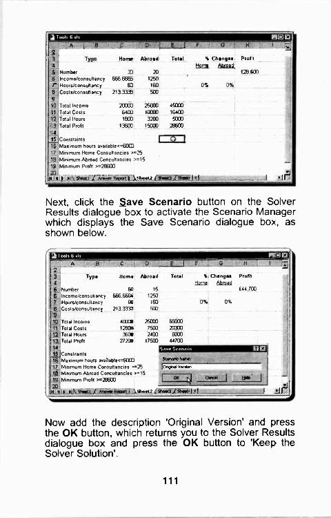
3 ! Type HOME Abroad Total Changes Prof t

4 Home Abroad

5 ,Number 20 f 26 500

6 ;Income/consultancy 656 666 1250

7 El 16011Hours/consultancy8 ,Costs/consuttancy 213 3333 503

910 Total Income 20003 25000 45=11 Total Costs 6403 10000 16403

12 , Total Hours 1807 3200 5000

131Tot al Profit 13603 15000 2E600

15 Constraints I16 Maximum hours available<=60CD17 'Minimum Home Consultancies >=2518 Minimum Abroad Concullancier )=1519 Minimum Profit >=2660320

4 4 .04 \Sabel ArmagatAapgallAshacqampl5haet,14 'U -

Next, click the Save Scenario button on the SolverResults dialogue bp): to activate the Scenario Managerwhich displays the Save Scenario dialogue box, asshown below.

ji tools 6 IdtB ID E H

23 Type4

Horn, Abroad Total % ChangsLigrni Abroad

5 Number 60 15

6 Income/consultancy 666 6666 1250

7 Hours/consultancy 60 160 0% 0%

El Costs/consultancy 213 3331 503

910 Total Income 400011 251300 651303

11 Costs 12808 75130 213300

12:Total Hours 3608 2403 6000

13 Total Profit 272011 17930 44700

14

15 Constraints16 Maximum hours available<=60C0 Scenario Nam

Profit

644 7[0

17 Minimum Horne Consultancies =Z Icipne versm18 Minimum Abroad Consultancies >='1519 Minimum Profit >=266111

204k NA *PAL( koa'lla!tPatl._),11.4.12 A 51,444904,'11__

Now add the description 'Original Version' and pressthe OK button, which returns you to the Solver Resultsdialogue box and press the OK button to 'Keep theSolver Solution'.

111

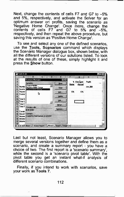
Next, change the contents of cells F7 anc G7 to -5%and 5%, respectively, and activate the Solver for anoptimum answer on profits, saving the scenario as'Negative Home Change'. Once more, change thecontents of cells F7 and G7 to 5% and 5%,respectively, and then repeat the above procedure, butsaving this version as 'Positive Home Charge'.

To see and select any one of the defined scenarios,use the Tools, Scenarios command wr ich displaysthe Scenario Manager dialogue box, shown below, withall the different versions of our solutions listed. To lookat the results of one of these, simply highlight it andpress the Show button.

sprain:4

5 Numb, C"°"`"'"""tiorne6 Inc o rn.

7 Hours,

8 costs,910 Total li11 Total C

12 Total F13 total F14

SCSS,SLIK515 Constr16 Ma,,rr Coment;17 m,n,,, Created by Noel Keetees on 6122197

10 I Minims I

19 Mtrom,20

% Changes 'tofuHome Abroad

i 44 268

AppenlaShert 2 / Sheet3 Sheet, 14 I

.5%

rJ

Last but not least, Scenario Manager alows you tomerge several versions together and define them as ascenario, and create a summary report - you have achoice of two. The first report is a 'scenario summary',while the second is a 'scenario pivot table'. With thepivot table you get an instant what -if analysis ofdifferent scenario combinations.

Finally, if you intend to work with scenarios, saveyour work as Tools 7.

112

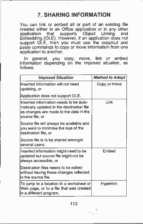
7. SHARING INFORMATION

You can link or embed all or part of an existing filecreated either in an Office application or in any otherapplication that supports Object Linking andEmbedding (OLE). However, if an application does notsupport OLE, the-) you must use the copy/cut andpaste commands to copy or move information from oneapplication to another.

In general, you copy, move, link o- embedinformation depending on the imposed situatior, asfollows:

Imposed Situation Method to Adopt

Inserted information will not needupdating, or

Application does not support OLE.

Copy or move

Inserted information needs to be auto-matically updated in the destination fileas changes are made to the data in thesource file, or

Source file will always be available andyou want to minimise tie size of thedestination file, or

Source file is to be shared amongstseveral users.

Link

Inserted information might need to beupdated but source fie might not bealways accessible, o,

Destination files needs to be editedwithout having these changes reflectedin the source file.

Embed

To jump to a location in a worksheet a-Web page, or to a file that was createdin a different program.

Hyperlink

113

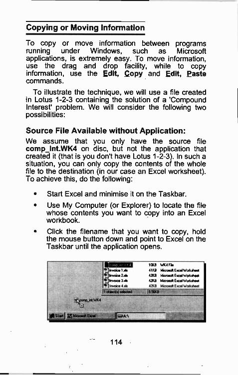
Copying or Moving Information

To copy or move information between programsrunning under Windows, such as Microsoftapplications, is extremely easy. To move information,use the drag and drop facility, while to copyinformation, use the Edit, Copy and Edit, Pastecommands.

To illustrate the technique, we will use a file createdin Lotus 1-2-3 containing the solution of a 'CompoundInterest' problem. We will consider the following twopossibilities:

Source File Available without Application:We assume that you only have the source filecomp_Int.WK4 on disc, but not the application thatcreated it (that is you don't have Lotus 1-2-3). In such asituation, you can only copy the contents of the wholefile to the destination (in our case an Excel worksheet).To achieve this, do the following:

Start Excel and minimise it on the Taskbar.

Use My Computer (or Explorer) to locate the filewhose contents you want to copy into an Excelworkbook.

Click the filename that you want to copy, holdthe mouse button down and point to Excel on theTaskbar until the application opens.

111 10KB WK4 Fie'llovorce 1 els 41KB Microsoft E see4Wakcheet

4lj Invoice 2 kis 42KB Microsoft Excel Wocksheet

4,11 Invoice 3 res 42KB Mocrosoe Excel Worksheet

411 Invoce 4 srs 42KB Microsoft E scel Worksheet

f TtioectisI Wooed WO*Lisornp_itWK4vLJ

.11111 Slut I ISMicooecit Email II k.1

114

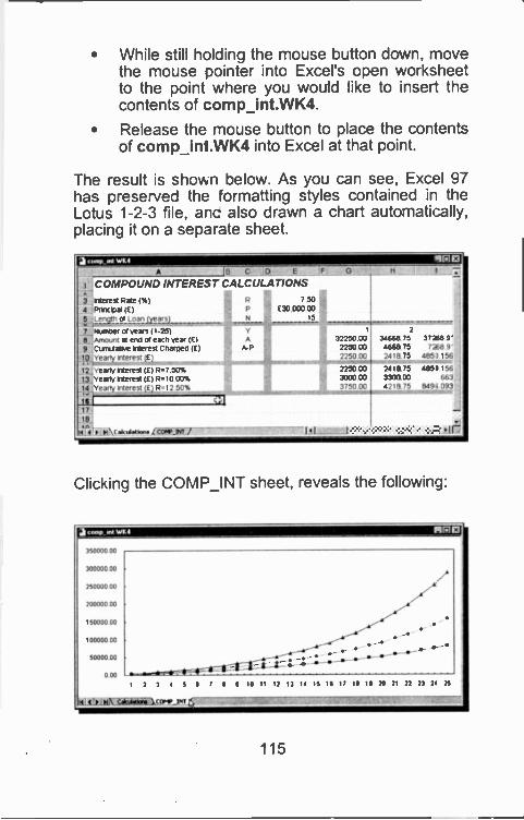
While still holding the mouse button down, movethe mouse pointer into Excel's open worksheetto the point where you would like to insert thecontents of comp_int.WK4.

Release the mouse button to place the contentsof comp_in1.WK4 into Excel at that point.

The result is shown below. As you can see, Excel 97has preserved the formatting styles contained in theLotus 1-2-3 file, anc also drawn a chart automatically,placing it on a separate sheet.

acomp int WJ.4

A 9 C O 6

CALCULATIONS

EIRE3

1 COMPOUND INTEREST3 ,r !,F.,- Pate % 7.504 to P E30.00000

N 15

7 Nurnoer or yews 11-251a:Amout at end or each year (E) AY 37250 00

2

3466875 37266 9'9 Cumulative Interest Charged (E) A -P 2250 00 466875 7Z. 9'1lifiVearty Interest (E) 2250 00 241875 4951 158

124Yearty Interest (E) R.7 50% 2250 00 241875 4953156'13 'Yearly interest (0) P.10 00% 3000 00 3300.00 663

1t +racy Interest (0, P '2 5,'14 3750 00 421875 8494 093

N 1 P d.,uto,. CCM_PIT 141 rlr

Clicking the COMP_INT sheet, reveals the following:

ro W1.4

350000 00

300000 00

250000 00

200000 00

150000 00

100000 00

5000000

000t 7 3 4 5 6 , 0 9 10 11 17 17 14 15 10 17 10 15 20 N 77 77 74 7S

kt-titillktaitailiatcvJrn -

115

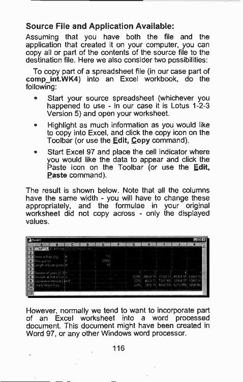
Source File and Application Available:Assuming that you have both the fi e and theapplication that created it on your computer, you cancopy all or part of the contents of the source file to thedestination file. Here we also consider two possibilities:

To copy part of a spreadsheet file (in our case part ofcomp_int.WK4) into an Excel workbook, do thefollowing:

Start your source spreadsheet (whichever youhappened to use - in our case it is Lotus 1-2-3Version 5) and open your worksheet,

Highlight as much information as you would liketo copy into Excel, and click the copy icon on theToolbar (or use the Edit, Copy command).

Start Excel 97 and place the cell indicator whereyou would like the data to appear and click thePaste icon on the Toolbar (or use the Edit,Paste command).

The result is shown below. Note that all the columnshave the same width - you will have to change theseappropriately, and the formulae in your originalworksheet did not copy across - only the displayedvalues.

EIMILIIIMplIMINIPINION11111111111=1111EININIIMINMINIMIIII

Ellfer11. I L

nJugef I,. of ,* lr i (1 T

,rout 4 end of olt AIM ,1 st ciAR

Inlef,r41 (n.f)

15.

em©

4,

3:2411 ' 4 .:16.1 37 .

ALL: 1C0.164 37: II)-24Io St -.4J I t 6.1.19114.

However, normally we tend to want to incorporate partof an Excel worksheet into a word processeddocument. This document might have been created inWord 97, or any other Windows word processor.

116

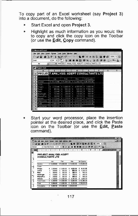
To copy part of an Excel worksheet (say Project 3)into a document, do the following:

Start Excel and open Project 3.

Highlight as much information as you woulc liketo copy and click the copy icon on the Toolbar(or use the Edit, Copy command).

Far Ea 41121:=71IMIIMIIIPI,..1.-.- ure 4. Vendw, tm.

n Lda, b a a v- X 4iff <I - t. ti t,4

-4-Itt IFillaf RCP% , fitjt - A.--j ,,p77 -Pf4A1 r 'I`; AE E P' r49_,CAN

Pooped 3 oh

Ill

1112

13

11

I E

A TPROJE

It

der APALTSJS: ADEPT CONSULTANTS LT

agesravel

ent

.14..9hteneira.ns

)1 11 ts

ten Feb Mar

16 000 00

I NatterE ono oof 1100 f 15.000 00 f

2.00 1113 E 3000 00 f 1000 00 i f 3,000 00f 110 f 500 00 f 600 00 f 1.500 00

Z10 110 f 300 00 f 300 E03 £ 930120

E ISO.) f 200 00 f 130 00 f 180 00

f SO 4. 300 00.4 350 00 f 900 ((If 1 130 NO f 12(0 00 f 1301(0 f 3 F.rn e,

£ 9 WO CO 950.000 f 93:000 f

Start your word processor, place the inse-tionpointer at the desired place, and click the Pasteicon on the Toolbar (or use the Edit, Pastecommand).

PInning g efe, IPPP POPP /Of Nib IMMO IPFOIP Oil 1/13k7 X ite rka -sop III.fas lo -.q]

lamasi ,M111 111 alums etsat IP o.,

PROJECT ANALYSE: ADEPTCONSULTANTS -TD

IS 12 11

Jan Feb kip I P

Inc on,* 111,000.00 £150®® f 161:0003 [KAMMCame

wage. fTravel IRIP f11Pkelff fPhoneff ma fAd. 0. I

2=034030030XIDISCPC1

250031,133

331300 fWO CO fKO CO fMI CO IMOO f

I AO 00 f

4W0 ffa0 3 fNO CO f132 CO L

MD 31.3 f

9 POD Of

I SCO CC

9000fPM CC

WOW3)933

Trr Cora I 4=03 SACCO f is9000 f IS.310121

Prey f 90303 L9A33 saoco n$2113Coonaambee f 'NOM f19.3413.00 I 30[.703

117

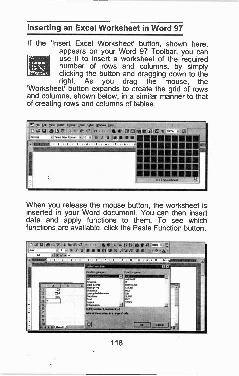
Inserting an Excel Worksheet in Word 97

If the 'Insert Excel Worksheet' button, shown here,appears on your Word 97 Toolbar, you canuse it to insert a worksheet of the requirednumber of rows and columns, by simplyclicking the button and dragging down to theright. As you drag the mouse, the

'Worksheet' button expands to create the grid of rowsand columns, shown below, in a similar manner to thatof creating rows and columns of tables.

int* Gdi Pa Pam FV jock Titie yrdc.. tiej,

Da PC? t15Ian .3 Cognac, -'*" - B I II 1"1" 11.11111111111111111_

=1Mili111111111117111....1111111111111..1111111111111111111.11.111111111111111,

6 a f fosaderst

When you release the mouse button, the worksheet isinserted in your Word document. You can then insertdata and apply functions to them. To see whichfunctions are available, click the Paste Function button.

D - ea IL ; IPA- 1 u sEsaM ay% .

123

231

99

ilitj t /

rurgten iptows rtrear peer

AKRAGEftannalDas 1101. MtVeViKWh I. r,o carer

a.Givrae

Sal51.1,

IROSit(

611.1(nunliml.savnb.V...)kidg V* rt.081011.rarp 016.

118

Object Linking and Embedding

Object Linking is copying information from one file (thesource file) to another file (the destination file) andmaintaining a connection between the two files. Wheninformation in the source file is changed, ther theinformation in the destination fi e is automat callyupdated. Linked data is stored in the source file, whilethe file into which you place the cata stores only thelocation of the source and displays a representation ofthe linked data.

For example, yon would use Ooject Linking if youwould want an Excel chart included in, say, a Worddocument to be updated whenever you changed theinformation used to create the chart in the first placewithin Excel. In such a case, the Excel worksheetcontaining the chat would be referred to as the sourcefile, while the Word document would be referred *.o asthe destination file.

Object Embedding is inserting information created inone file (the source file) into another file (the containerfile). After such infcrmation has been embedded, theobject becomes part of the container file. When youdouble-click an embedded object, it opens in theapplication in which it was created in the first place.You can then edit it in place, and the original object inthe source application remains unchanged.

Thus, the main differences between linking andembedding are wl-ere the data is stored and how it isupdated after you place it in your file. Linking savesyou disc space as only one copy of the linked object iskept on disc. Embedding a logo chosen for yourheaded paper, saves the logo with every saved letter!

In what follows, we will discuss how you can link orembed either an entire file or selected information froman existing file, anc how you can edit an embeddedobject.

119

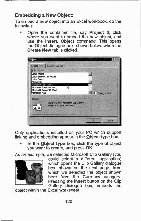
Embedding a New Object:To embed a new object into an Excel workbook, do thefollowing:

Open the container file, say Project 3, clickwhere you want to embed the new object, anduse the Insert, Object command. This opensthe Object dialogue box, shown below, when theCreate New tab is clicked.

Object 1E1E3

Create New I Create from File

Abject type:

Lotus MediaLotus Su eenCarn MovieLotus SoundMedia C

IliCrOSOrr

Microsoft Equation 3.0Microsoft Graph 97 ChartMicrosoft Map

Inserts a new Microsoft Clip Gaieryobject into your document.

r- Nsplay as Icon

OK Cancei

Only applications installed on your PC which supportlinking and embedding appear in the Object type box.

In the Abject type box, click the type of objectyou want to create, and press OK.

As an example, we selected Microsoft Clip Gallery (youcould select a different application)which opens the Clip Gallery dialoguebox, shown on the next page, fromwhich we selected the object shownhere from the Currency category.Pressing the Insert button on the ClipGallery dialogue box, embeds the

object within the Excel worksheet.

120

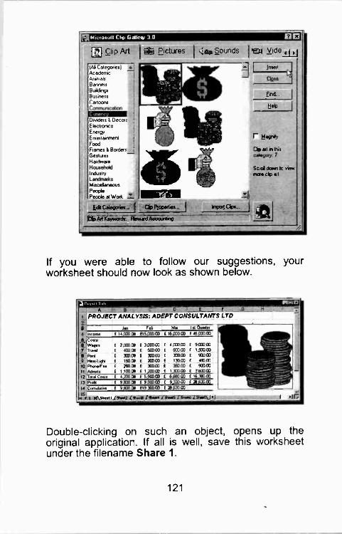
tgiMicsosoft Chp Gallen. 3 0 E3

Cetegooes1Ac &demoAnmahB anonBaldngsBusnes:CedoonsI arm:re-don

Oman Deca:EleceorscsEreigyEntedanmentFoodFlames I BadenGestaes

He:c.:seHousehadI raahyLandmanMiscellaneousPeoplePeooie d Work

Edit Cali:gain...

is Pictures ,. founds I .04 V ideild

apPtcostbis--

Alt *peva*. Reward Acme/sing

WWI CIPL-

MEE!apse

foil..

Netbet.

r Magnify

Clip eat n th:sFYISc oil dawn tc viewmos cip art

4_11

If you were able to follow our suggestions, yourworksheet should now look as shown below.

A 9 Q D E

I PROJECT ANALYSIS: ADEPT CONSULTANTS LTD

3voint

5'word6 Word

6 vim9 P.sodulogN

W PtIonefftt Ad.11.12 1 alai Coals

Pp,4.1

Id vr,Jidt.

J. Feb Mel Ouddir

11)333 CS 71 SITE CID 16)10 CC Kftil 771

.0:11 CM 3111303 4 DEO CO 9!100 CO

CO CO KIM 6030 1533 CO

300 01 300 00 33300 900001504 71300 13003 MO GO

250 CM 3131:0 36000 933331 103 1,203 Co 1,300 00 3pto

70001 5 503 00 6300 CO 16,70000

9300 01 9 5C0 CO 9,320 03 33,533 CO

9)300 M 19 XD CO 867033

Nye14 4 \ Fort: P.m° /9,.e. 9.. 9.64 /Shoe, I

Double-clicking on such an object, opens up theoriginal applicatior. If all is well, save this worksheetunder the filename Share 1.

121

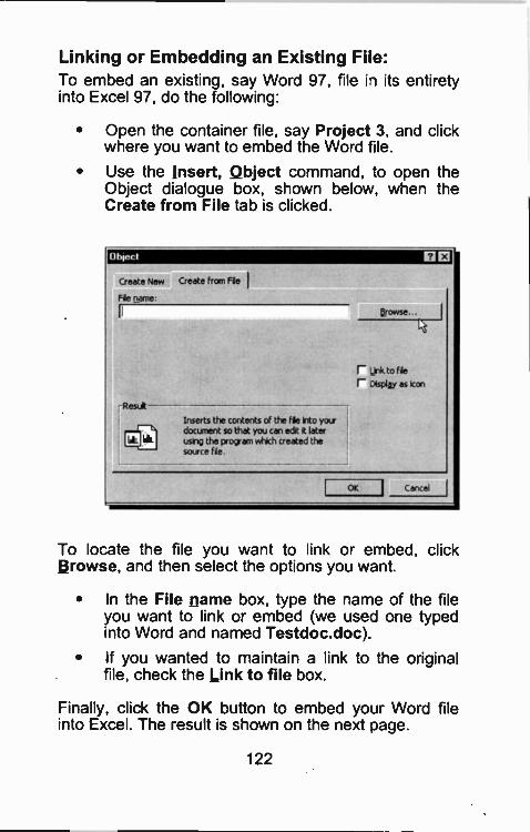
Linking or Embedding an Existing File:To embed an existing, say Word 97, file i its entiretyinto Excel 97, do the following:

Open the container file, say Project 3, and clickwhere you want to embed the Word file.

Use the Insert, Object command, to open theObject dialogue box, shown below, when theCreate from File tab is clicked.

Object

Create New Create from File

File name:

ri

Result

Inserts the contents of the fie Into yourdocument so that you can edit it laterusing the program which created thesource file.

afowse. I

r ;.ink to fier Display as icon

OK Cancel

To locate the file you want to link or embed, clickBrowse, and then select the options you want.

In the File name box, type the name of the fileyou want to link or embed (we used one typedinto Word and named Testdoc.doc).

If you wanted to maintain a link to the originalfile, check the Link to file box.

Finally, click the OK button to embed your Word fileinto Excel. The result is shown on the next page.

122

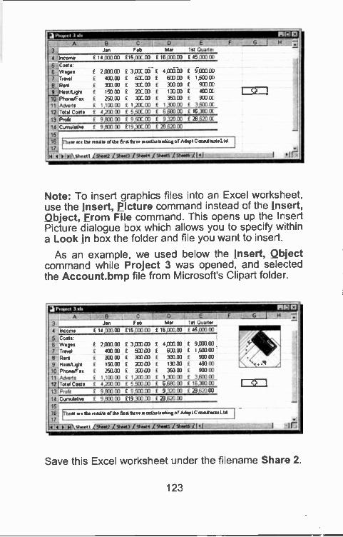
a Peeled 3.1r EnT F2

A C F G H

3 Feb Mal

4 ,Incorne f 14 CO 1.! f 15 BCC DO f 16000 00 f 45 flOO Of

.54 Costs6 Wages E 2,0:0 00 f 3,000 03 E 4.000 00 E 9,000 130

Travel £ 400 00 f S:C130 f 600 oo £ 1,500 OE

Rent £ 31100 f 31.03 £ 30000 £ 900 OE_ILX HeatAight £ 150.00 £ 20L00 f 133 00 f 480 IX

Ilk Phone/Fax f 250.00 f 30000 £ 350 00 £ 900 CC

11 Adverts E 1,10003 f 1,20000 £ 1,3:000 f 36000E

13 Total Costs £ 4,200 CO £ 5,50000 E 6)330 00 f 16,333 Of

13 Profit f 9,800 00 £ 9,5CC00 £ 9,320 00 £ 28,620 OE

14 Cumulative f 9,833 00 f19,33L CO f 28520 CO

15

11 tha results of tha first Seta 12 orito Ise:knot Adapt Colorant:ea Ltd

l411.11_41Nsh.et I 1 177

Note: To insert graphics files into an Excel worksheet,use the Insert, Picture command instead of the Insert,Object, From File command. This opens up the InsertPicture dialogue box which allows you to specify withina Look in box the folder and file you want to insert.

As an example, we used below the Insert, Objectcommand while Project 3 was opened, and selectedthe Account.bmp file from Microsoft's Clipart folder.

3 Jan Fab Mar 1st Quartet

4 Income f 1403300 £151:0000 £ 1600303 f 45133300

J Costs'6 £ 2,1330.00 £ 3000130 £ 4033.00 f 9=00,Wages

'Travel £ 400 M f 5 100 f 600.00 f 1,500 00.79 Pent £ 300E0 £ 33303 f 333.03 910 03

9 Heat/Light f 19000 f 3000 f 13103 f 480 133

10:Phone/Fax f 26003 £ 333130 f 36003 f 90000

11 Adverts f11013Mf1 C0f3 M12 Total Costs f 4 11.03 f 503310 £ 6:;a.0 f 16 00

13 Profit £ 9,800 00 f 9,50303 E 9,320 M £ 23,620 03

14 Cumulative £ 9,800.03 f19,33310 f 26620.03

1516

17

Thmss the mutts rigs. fu a twee a °rah' tradtogof Adapt C aniulheta Ltd

Sheet 7.148:Ligiii 1 11 21t.;

Save this Excel worksheet under the filename Share 2.

123

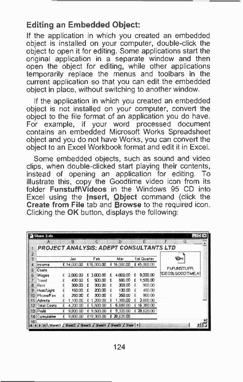
Editing an Embedded Object:If the application in which you created an embeddedobject is installed on your computer, double-click theobject to open it for editing. Some applications start theoriginal application in a separate window and thenopen the object for editing, while other applicationstemporarily replace the menus and toolbars in thecurrent application so that you can edit the embeddedobject in place, without switching to another window.

If the application in which you created an embeddedobject is not installed on your computer, convert theobject to the file format of an application you do have.For example, if your word processed documentcontains an embedded Microsoft Works Spreadsheetobject and you do not have Works, you can convert theobject to an Excel Workbook format and edit it in Excel.

Some embedded objects, such as sound and videoclips, when double-clicked start playing their contents,instead of opening an application for editing. Toillustrate this, copy the Goodtime video icon from itsfolder Funstuff\Videos in the Windows 95 CD intoExcel using the Insert, Object command (click theCreate from File tab and Browse to the required icon.Clicking the OK button, displays the following:

a Shale 3 xls

A

PROJECT ANALYSIS: ADEPT CONSULTANTS LTD

3 , Jan

4 ;Income f 14,000 00

9I Costs6, Wages £ 2.000 CO

7 Travel £ 400 009 J Rent £ 300 039 i Heat/light £ 150.03

1131Phone/Fax £ 250 0311 -,Adverts f 1,1000312 Total Costs f 4,200 00

Feb Mar 1st Quarter

£1530000 £ 16,000.00 £ 45,003 00\ FUNSTUFF\

f 300000 £ 4,000.00 £ 9000.00 IDEOSG00011MEA`

f 503.00 f 603.(XI £ 1,500.00

f 10.00 £ 300.00 £ 930.03f 203.00 f 133.00 £ 483.00

f 303 03 £ 350.00 £ 900 00£ 1,200.00 £ 1,300.00 £ 3500.00f 5 500 00 f 6 680 03 f 16.380 00

13 Profit f 980000 £ 9.83303 £ 932000 £286200014 Cumulative £ 9 800 00 £19 300 03 f 28 6213 00

Sheet! Lin .4.7thimet _,a_rost4 l glets_i _J IA

124

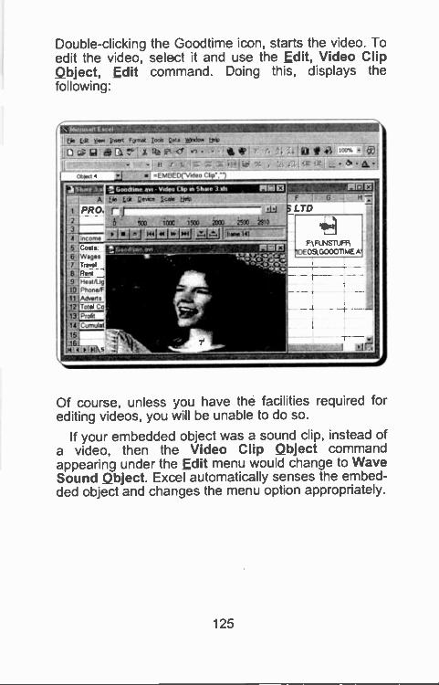
Double-clicking the Goodtime icon, starts the video. Toedit the video, select it and use the Edit, Video ClipQbject, Edit command. Doing this, displays thefollowing:

lith EI Vow livot Firma 'oda 444. belp

lb au a as. ..? :, X % i'k Cr .n 10, #i , : , 111 f 43 ; pox fi) !

. - if i t ':_ - . - . ILI^ -F Mort 4 if f MET OrVorleo C hp' "1

.1Sh. . 51 400dinee ay, Voclea Clip on Sham 3 .1, PIE E3A tie LcR Dim:. Icasi boo

An©F t

t

I PRO. r) lia,:. LTD2 6 soo km ism iom isoo Ir) 4;

Incomi l "41 44 I* !WI .=_21A..1 riti-o-o 141

.Cools RErwars - --- -------uramusor..I 7--

F.% FUNS1UFK09,C.00011MEN

...m....x.t.eTrost ...a KZ...,RentHoot/4PhonsofAthelsTotal . JProfs

14 rn

1,1SIctol 4 I' V. - I il r'7.

Of course, unless you have the facilities required forediting videos, you will be unable to do so.

If your embedded object was a so,ind clip, instead ofa video, then the Video Clip Qbject commandappearing under the Edit menu would change to WaveSound Qbject. Excel automatically senses the embed-ded object and changes the menu option appropriately.

125

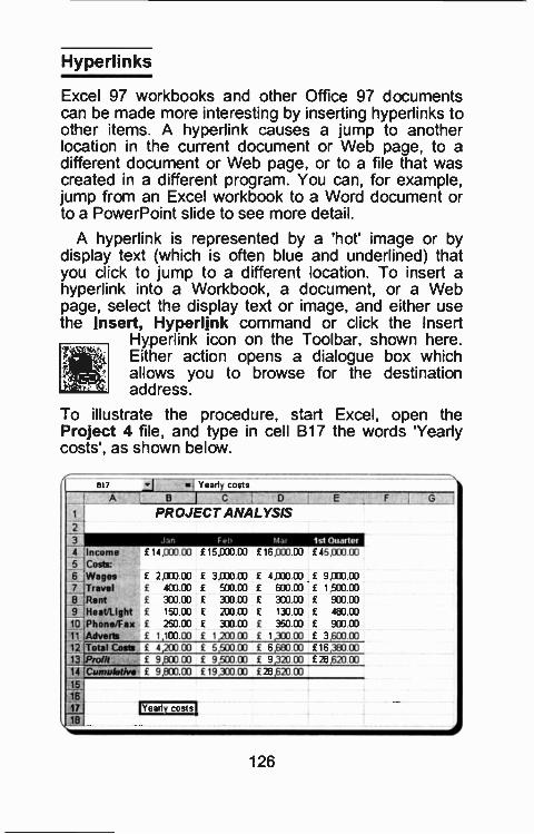
Hyperlinks

Excel 97 workbooks and other Office 97 documentscan be made more interesting by inserting hyperlinks toother items. A hyperlink causes a jump to anotherlocation in the current document or Web page, to adifferent document or Web page, or to a file that wascreated in a different program. You can, for example,jump from an Excel workbook to a Word document orto a PowerPoint slide to see more detail.

A hyperlink is represented by a 'hot' image or bydisplay text (which is often blue and underlined) thatyou click to jump to a different location. To insert ahyperlink into a Workbook, a document, or a Webpage, select the display text or image, and either usethe Insert, Hyperlink command or click the Insert

Hyperlink icon on the Toolbar, shown here.Either action opens a dialogue box whichallows you to browse for the destinationaddress.

To illustrate the procedure, start Excel, open theProject 4 file, and type in cell B17 the words 'Yearlycosts', as shown below.

617 - .1 Yearly costsA B I C 1 01

PROJECT ANALYSIS2

3 1s1 Ouarter

4 Income £ 14,000 00 £ 15,000 00 £ 16,000 00 £ 45,000 00

5 Costs:jWages £ 2,000 00 £ 3,000 00 £ 4,000 00 £ 9,000 DO

£ 403 00 £ 503 03 £ 600 CID £ 1 ,503 00

8 'Rent £ 300 00 £ 333 013 330 00 £ 900 009 HeaVLight £ 150 0i3 £ 200 00 £ 133 00 480 0010 Phone/Fax £ 250 00 £ 333 00 £ 350 00 £ 900 0011 Adverts £ 1,100 00 £ 1,2013 00 1,333 00 £ 3,600 0012 Total Costs £ 4,200 00 £ 5,500 00 £ 6,680 00 16,360 0013 1.profii £ 9,6013 00 £ 9,500 00 9,320 00 £ 28,620 0014 Cumuiethm £ 9,600 00 £ 19,333 00 £ 28,620 013

15

16

17 Yearl costs

126

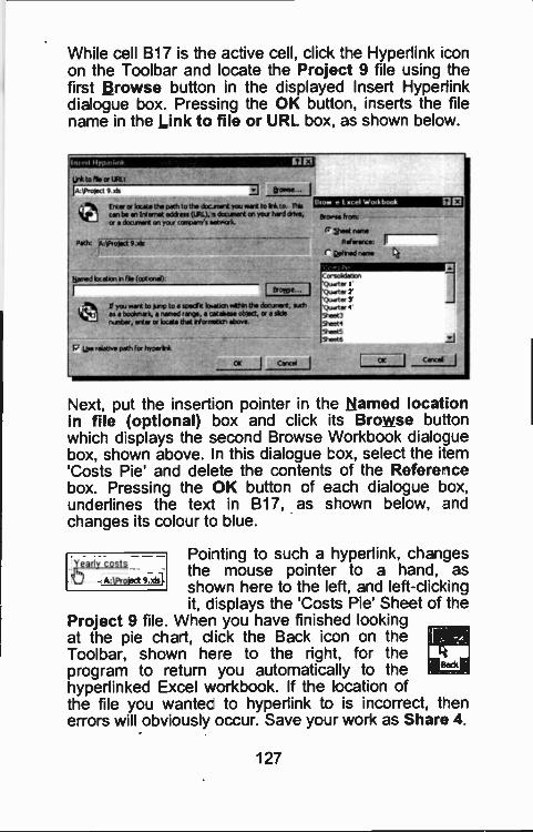
While cell B17 is the active cell, click the Hyperlink conon the Toolbar and locate the Project 9 file using thefirst Browse button in the displayed Insert Hype -linkdialogue box. Pressing the OK button, inserts the filename in the Link to file or URL box as shown below.

Int ell tlypenlank

Unk to Ms or URI:

Ia P.oie.ct 9 xls

Enter or locate Orwell to the docsoent you mint to Ink to. fidecan be an Internet adieu (MO,. dowel ch you hard dive,or donhont on yoLe comany's setecek.

Path: A AProject 9.ets

I

rod batonh Ile (olonel):

Bronx-. 1

I you vent to ;top to a speck b.aton Whin the decor et, so&as a booloorkda named range, a oatabese object, or e fadenumber, enter or bate let Homan above.

greatly, path fce hvorInk

_1 Cecil

throw e Lecd Workbook gelDrool* hove

5ireet retro

Reference: 1[

r &feed neve

1.11121.111111.....11.1117.forscidabonQuarts I'Que.'Quarts 3''Quote. o'9.30Setagirt`9-.46

OK Cancd

Next, put the insertion pointer in the Named locationin file (optional) box and click its Browse buttonwhich displays the second Browse Workbook dialoguebox, shown above. n this dialogue box, select the item'Costs Pie' and delete the contents of the Refere icebox. Pressing the OK button of each dialogue box,underlines the text in B17, as shown below, andchanges its colour to blue.

easa,512

A:kProgct 9.Ad

Pointing to such a hyperlink, changesthe mouse pointer to a hand, asshcwn here to the left, and left. -clickingit, cis plays the 'Costs Pie' Sheet of the

Project 9 file. When you have finished lookingat the pie chart, click the Back icon on the it1-4Toolbar, shown here to the righ-., for the kprogram to return you automatically to the "61hyperlinked Excel workbook. If the location ofthe file you wantec to hyperlink to is incorrect, teenerrors will obviously occur. Save your work as Share 4.

127

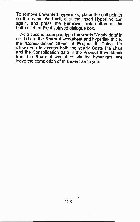
To remove unwanted hyperlinks, place the cell pointeron the hyperlinked cell, click the Insert Hyperlink iconagain, and press the Remove Link button at thebottom left of the displayed dialogue box.

As a second example, type the worc s 'Yearly data' incell D17 in the Share 4 worksheet and hyperlink this tothe 'Consolidation' Sheet of Project 9. Doing thisallows you to access both the yearly Costs Pie chartand the Consolidation data in the Project 9 workbookfrom the Share 4 worksheet via the hyperlinks. Weleave the completion of this exercise to you.

128

8. USING MACROS

In Excel 97 and other spreadsheet packages, you canautomate tasks or create complete applications bywriting macros. A macro is simply a set of instructionsmade up of a sequence of keystrokes. mouseselections, or commands which, in the case of Excel 97are stored in a Visual Basic module. After saving, orwriting, a macro and attaching a quick key combinationto it, you can run the same sequence of commandswhenever you want. This can save a lot of time and,especially with repetitive operations, can save mistakescreeping into your work.

In Excel there are two basic ways of creatingmacros. The first oie involves the use of Visual Basic,the programming language that is common to all Office97 applications. Witt-, this method, you can write quitecomplex macro programs directly into a macro fileusing the Visual Basic Editor which allows you to editmacros, copy macros from one module to another,copy macros between different workbooks, rename themodules that store the macros, or rename the macros.Understanding Visual Basic makes it easier to alsoprogram with other Microsoft applications that use thelanguage.

For simple work however, you don't really have tolearn to program in Visual Basic, as Excel includes aMacro Recorder which provides you with the secondmethod of generating macros. The Macro Recorderstores the actions you take and the commands you usewhile working with Excel, which can then be playedback (run) to repeat the recorded actions andcommands.

Before you record or write a macro, plan the stepsand commands you want the macro to perform. This isessential, because you make a mistake when yourecord the macro, corrections you make will also berecorded. Each time you record a macro, the macro isstored in a new module attached to a workbook.

129

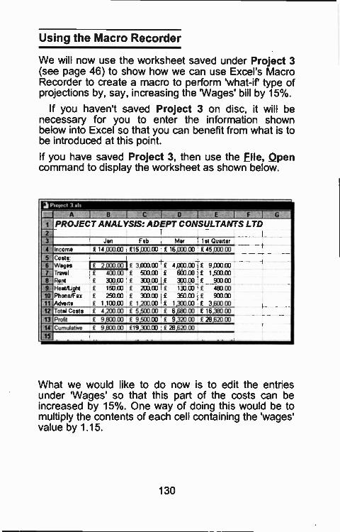
Using the Macro Recorder

We will now use the worksheet saved under Project 3(see page 46) to show how we can use Excel's MacroRecorder to create a macro to perform 'what -if type ofprojections by, say, increasing the 'Wages' bill by 15%.

If you haven't saved Project 3 on disc, it will benecessary for you to enter the information shownbelow into Excel so that you can benefit from what is tobe introduced at this point.

If you have saved Project 3, then use the File, Opencommand to display the worksheet as shown below.

2 Pioled 3.xls

A I B I C CI I E IF ll G

1 PROJECT ANALYSIS: ADEPT CONSULTANTS LTD23 Jan Feb Mar 1st Quarter

4 Income f 14,000 00 £15,000 00 £ 16,000 00 f 45,000 005 Costs6 Wages 1 f 2,000.00 If 3,000 CO £ 4,000 00 £ 9,000 007 Travel £ 400 00 f 500 00 f 600 CC £ 15013 008 Rent £ 330.00 £ 300.00 £ 300.00 £ 900 009 Heat/Light £ 150 00 £ 200 00 £ 133 DI] £ 480 0010 Phone/Fax £ 250.130 £ 33003 f 350.00 £ 90001311 Adverts f 1,100 00 f 1200 03 f 1,333 00 f 3,600 010

12 Total Costs £ 4,203 03 £ 5,500 00 £ 6,68000 f 16,380 00

13 Profit £ 9,800 00 £ 9,50000 £ 9,320 00 £ 28,620 00

14 Cumulahve £ 9,800 00 £19,300 00 £ 28620.0015

What we would like to do now is to edit the entriesunder 'Wages' so that this part of the costs can beincreased by 15%. One way of doing this would be tomultiply the contents of each cell containing the 'wages'value by 1.15.

130

To do this, we would start by changing the contents ofcell B6 into a formula, by pressing the F2 function keyto 'Edit' the value in it by adding an equals sign at thebeginning of the entry and then typing '1.15' at the endof it, which has the effect of multiplying the contents ofthe cell by 1.15, thus increasing its contents by 15%.We would then press the <Enter> key which wouldcause the cell pointer to drop to B7, press the T arrowkey to move back lo cell B6, then press the -> arrowkey to move to cell C6 and repeat the wholeprocedure. The exact steps, after highlighting cell B6,are as follows:

Manual ProcedurePress F2 to 'Edit' celPress the <Home> key to move to beginning of entryType = to change entry to formulaPress <End> to move to the end of the entryType *1.15Press the <Enter> keyPress T arrow keyPress -> arrow key.

Recording an Excel 97 Macro:Having opened the Project 3 file, highlight cell B6 - thefirst cell we want to operate on. Then, select the Tools,Macro, Record New Macro command which displaysthe Record Macro cialogue box with the default Macroname given as Macrol. This can be changed by you tosome more meaningful name, if you so wished.

In the Record Macro dialogue box, we specified thatthe Shortcut key should be Ctrl+w (w for wages), asshown on the scree I dump on the next page.

131

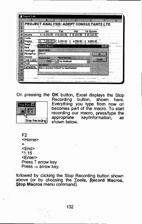
ji holed 3 xl:A B C I D

PROJECT ANALYSIS: ADEPT CONSULTANTS LTD213 j Jan Feb Mar 1st Quarter4 Income f 14 WO III £15 000 00 f 16 COO 13:1 f 45 000 005 Costs6 Wages7 Travel

13_1Rent

0_,Heat/Light10 'Phone/Fax11 .Adverts12 Total Costs

13 ,Profit

14 .Cumulative

15116

17

f 2 000 00 £ 3,000 00 f 4,000 DJ f 9,000 00- .Record Mac n©dacro name:

IMecrol

Shortcut ipy: 'Rae macro

ctr1471 ITkvs Workbook

Dri$CrOton:

recto recorded 1`,106;97 by "loci Kent ears

On pressing the OK button, Excel displays the StopRecording button, shown here.Everything you type from now onbecomes part of the macro. To startrecording our macro, press/type theappropriate key/information, as

Stop Recording shown below.

Stop Recel

F2<Home>

<End>*1.15<Enter>Press T arrow keyPress arrow key.

followed by clicking the Stop Recording button shownabove (or by choosing the Tools, Record Macros,stop Macros menu command).

132

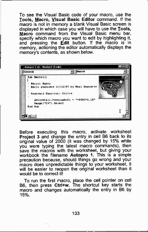
To see the Visual Basic code of your macro, use theTools, Macro, Visual Basic Editor command. If themacro is not in memory a blank Visual Basic screen isdisplayed in which case you will have to use the Tcols,Macro command from the Visual Basic menu bar,specify which macro you want to ecit by highlighting it,and pressing the Edit button. If the macro is inmemory, actioning the editor automatically displays thememory's contents. as shown below.

,; Aulopio 1 xls - Modulel (Code) MOM

kin LI I Alec r 012:1

Sub Naerol()

Meicrol Macro. "'

Macro recorded 1E/C6/97 by Noel Kantaris Anel-,, 0 - . \

170(YeyLoatJ Shortcut: Ctr 1 -,:.;44:::6

Act lyeCell . FornulaR1C1 - "2000*1 . 15"

Range("C6").SelectEnd Sub

ji

Before executing this macro, activate worksheetProject 3 and change the entry in cell B6 back to itsoriginal value of 2000 (it was charged by 15% whileyou were typing the latest macro commands), Thensave the macros with the worksheet, but giving yourworkbook the filename Autopro 1. This is a simpleprecaution because, should things go wrong and yourmacro does unpredictable things to your worksheet, itwill be easier to reopen the original worksheet than itwould be to correct it!

To run the first macro, place the cell pointer on cellB6, then press Ctrl+w. The shortcut key starts themacro and changes automatically the entry in B6 by15%.

133

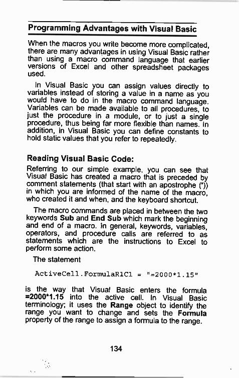
Programming Advantages with Visual Basic

When the macros you write become more complicated,there are many advantages in using Visual Basic ratherthan using a macro command language that earlierversions of Excel and other spreadsheet packagesused.

In Visual Basic you can assign values directly tovariables instead of storing a value in a name as youwould have to do in the macro command language.Variables can be made available to all procedures, tojust the procedure in a module, or to ust a singleprocedure, thus being far more flexible than names. Inaddition, in Visual Basic you can define constants tohold static values that you refer to repeatedly.

Reading Visual Basic Code:Referring to our simple example, you can see thatVisual Basic has created a macro that is preceded bycomment statements (that start with an apostrophe ('))in which you are informed of the name of the macro,who created it and when, and the keyboard shortcut.

The macro commands are placed in between the twokeywords Sub and End Sub which mark the beginningand end of a macro. In general, keywords, variables,operators, and procedure calls are referred to asstatements which are the instructions to Excel toperform some action.

The statement

ActiveCell.FormulaR1C1 = "=2000*1.15"

is the way that Visual Basic enters the formula=2000*1.15 into the active cell. In Visual Basicterminology; it uses the Range object to identify therange you want to change and sets the Formulaproperty of the range to assign a formula to the range.

134

An 'object' is something you control in Visual Basic.Each object has characteristics called 'properies'which control the appearance of the object. Objectsalso have 'methods' which are actions that they cantake.

In Visual Basic, you use:

Objects (such as Workbooks, Worksheets,Ranges, Charts) to perform a task. Each objecthas characteristics, called properties, that makethat object useful by controlling the appearanceor behaviour of an object.

Properties (such as ActiveCell, ActiveSheet,Value, Selection, ColumnWid:h, RowHeight), toexamine the condition of an object by returningthe value of ore of the object's properties (suchas a character string for Value, a numeric valuefor ColumnWid:h, True, or False).

Methods which are actions that objects can do(such as Calculate, Clear, Copy, Justify, orTable). Methods are a part of objects just likeproperties. The difference between them is Thatproperties have values which are set or returred,while methods are actions you would like anobject to perform.

Should you want tc learn to program in Visual Basic,then may we suggest you start with the bookProgramming in Visual Basic for Windows (13P346),also published by BERNARD BABANI (publishing) Ltd.

135

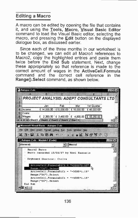
Editing a Macro

A macro can be edited by opening the file that containsit, and using the Tools, Macro, Visual Basic Editorcommand to load the Visual Basic editor, selecting themacro, and pressing the Edit button on the displayeddialogue box, as discussed earlier.

Since each of the three months in our worksheet isto be changed, we can edit all Macrol references toMacro2, copy the highlighted entries and paste themtwice before the End Sub statement. Next, changethese appropriately so that reference is made to thecorrect amount of wages in the ActiveCell.Formulacommand and the correct cell reference in theRange().Select command, as shown below.

2 Aulook 2 -xis FIR elA 13 C

. ._..!......_ E 1,41L.i:1 PROJECT ANALYSIS: ADEPT CONSULTANTS LTDI2 ii3 Jan Feb Mar 1st Ou3rter4 Income E 14,000 00 E 15 ,000 00 £ 16,000 00 E 45,003 005 Costs6 I Wages £ 2,300 00 £ 3,450 00 £ 4,600 00 f 10 393 00

14 4 Stijii\Cet1 Sheet2 Z Shea'! Shat4 Stool 4 I

da Micsosoll Visual Bask - Aulopio 2 .1. PIE3 elFi,, cat vie. Insert Fgrrnat Qeboo gin 1001s_rndOW U al p

i

za- IA t) e OA ..--) II NM N."'S--'!;Aulciplo 2. xls Modukl (Code) MCI IE3kGemssa4 J IMmoo2 2j

' Macro2 NEWT( jj' Macro recorded 15/06/97 by Noel Kanterls

F=yb,,,Ard :11ort,-,u.': Crri+v

2

ActiveCell.ForinulaP1C1 = "=2000.1.15.Pangef"C6").SelectActiveCell.FormulaR1C1 = "=3000.1.15"Range("D6").SelectActiveCell.TormulaR1C1 = ==4000.1.15"Range("E6").Select --

End Sub

011-1 A136

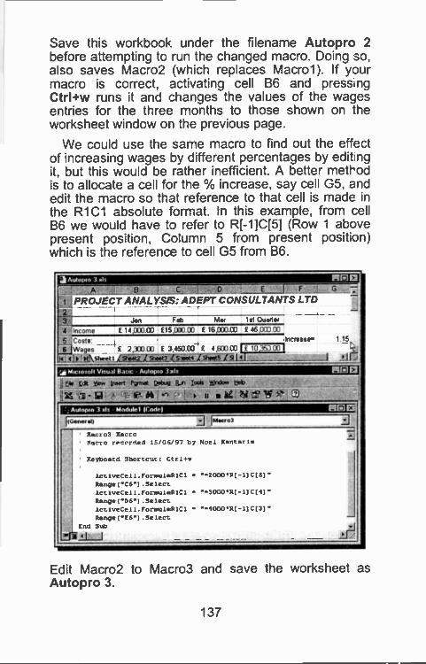
Save this workbook. under the filename Autopro 2before attempting to run the changed macro. Doing so,also saves Macro2 (which replaces Macro1). If yourmacro is correct, activating cell B6 and press ngCtrl+w runs it and changes the values of the wagesentries for the three months to those shown on theworksheet window on the previous page.

We could use the same macro to find out the effectof increasing wages by different percentages by edit ngit, but this would be rather inefficient. A better methodis to allocate a cell for the % increase, say cell G5, andedit the macro so that reference to that cell is made inthe R1C1 absolute format. In this example, from cellB6 we would have to refer to R[ -1]C[5] (Row 1 abovepresent position, Coumn 5 from present position)which is the reference to cell G5 from B6.

jiAtiopto 3 Os PER El

8 L C._ -q.. , 0 E I F 7.. -A j PROJECT ANALYSIS: ADEPT CONSULTANTS LTD -

. _Jan Feb Mar 1st Quarter

I Income £ 14,000 00 f 15 ,030 03 f 16,000 00 f 15,003 00

5 :Costs Increase= 1 15

IjitiVages f 2,303 00 f 3,450 00 f 4 Eat CO f 10 00

14-:.5 letNsh.-.11,CtigtiNI*7-2-1Weiillhast-s-rt 14 !JO.4 MICI01011 Visual Banc Aulopoo 361s RR El

it EN Lot Yew - F17,61 Lab* R.K. rods Wilda* lialtr

* -a - 61 ' ii" 04 .r+ : r he ' kii 6' W.. Allift/WO 3 als - Modulel rode( MCI

IIGeners1) A II/sego) -Maud': Me,14.

' Macro recorded 15/06/97 b7 Noel Kalmar la -' Keyboard Shortcut: Ctr 1+a

Act 1veCe 1 1 . rormulaR17.1 "-2000P(-11C(5) "Range ("C6") .5e lect.Act IveCe 1 1 . forroulaR1.71 "3000R( -11C ( 4) "Range ("66") . Se lect.Act isreCei i . formuied0:3. . "1000R( - I) C ( 3) "Range ("C6") . Se lect. -

End SubI L. j

Edit Macro2 to Macro3 and save the worksheet asAutopro 3.

137

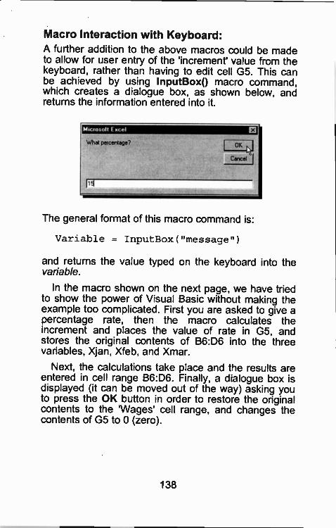
Macro Interaction with Keyboard:A further addition to the above macros could be madeto allow for user entry of the 'increment' value from thekeyboard, rather than having to edit cell G5. This canbe achieved by using InputBox() macro command,which creates a dialogue box, as shown below, andreturns the information entered into it.

The general format of this macro command is:

Variable = InputBox("message")

and returns the value typed on the keyboard into thevariable.

In the macro shown on the next page, we have triedto show the power of Visual Basic without making theexample too complicated. First you are asked to give apercentage rate, then the macro calculates theincrement and places the value of rate in G5, andstores the original contents of B6:D6 into the threevariables, Xjan, Xfeb, and Xmar.

Next, the calculations take place and tie results areentered in cell range B6:D6. Finally, a dialogue box isdisplayed (it can be moved out of the way) asking youto press the OK button in order to restore the originalcontents to the 'Wages' cell range, and changes thecontents of G5 to 0 (zero).

138

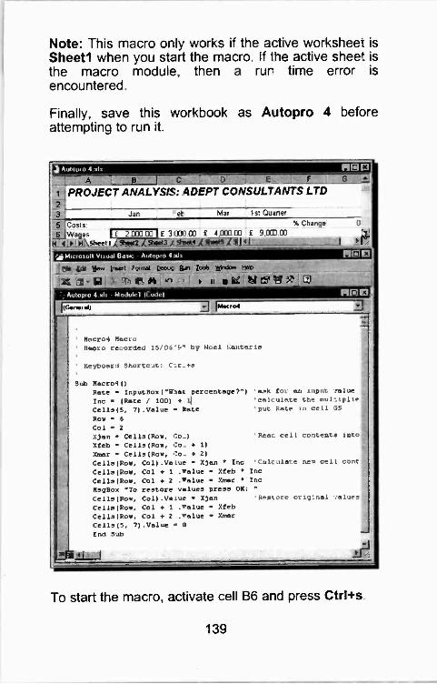
Note: This macro or ly works if the active workshee-. isSheet' when you start the macro. If the active sheet isthe macro module, then a rur time error isencountered.

Finally, save this workbook as Autopro 4 beforeattempting to run it.

2 Auloom 4.idt NEI CIA B IC D E F G

1 PROJECT ANALYSIS: ADEPT CONSULTANTS LTD2

3 Jan et Mar 1st Coale.

5 Costs % Change

6 !Wages 1£ 2000 00 I f 3 OM 00 f 4,00000 f 9(000N 1111211NSheetheeit3_A Sfilet4 51 ikiii=114439 4 1

14

-_,A 1ciesolt Visual Basic Autopto (ids SE©

Els La %w Insert Egonat Debuc Ran Dols }tend..., Net,

Z 61 - 12 ' P A ', 1 i 1 ke NI 'Iq' -;,... t!,- Autopro 4 ds - Module' 'Code) An ElI(Genera) zj P.M. o.4

2.21121_1

L.-

' Macro recorded 15/06'9' by Noel Kantaris

' Keyboard Shortcut: C--r-fa

Sub Macro4 0Rate - InputBox ("W 1st pereentage)v) 'ask for an input falueInc - (Rate / 100) + 11 'calculate the laul-.1p11.Celle(5, 7).Velue .. Rate 'put Rate in cell 05Rov v 6

Col . 2

Klan - Cells(Rov, .:o..) 'Peet cell contents int ,Xteb - Cells(Rov, ,:o- + 1)laser - Cells(Rov, Co_ + 2)Cells (Rov, Col) .Va Luc - Xjen Inc 'Calculate new cell cnnt

,

Cells(Rov, Col + 1 . value - Xteb IncCells(Rov, Col + 2 .value - Xxxar IncKsgBox ^To restore values press OK: "

Cells(Rov, Col) .Vik.ue X)an ,...., .-.re original val,Cells(Rov, Col + 1 .value - XfebCells(Rov, Col + 2 .value - XrnarCel Is (5, 7) .Value 0End Sub -

AC"-

To start the macro, activate cell B6 and press Ctrl+s

139

Visual Basic has many more statements, commandsand functions which can be used to build and run yourapplication in special ways. What we have tried to dohere is to introduce you to the sub.ect and give yousome idea of the power of this programming language.A fuller explanation of Visual Basic is beyond the scopeof this book.

140

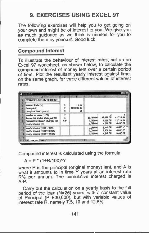
9. EXERCISES USING EXCEL 97

The following exercises will help ycu to get going onyour own and might be of interest to you. We give youas much guidance as we think is needed for you tocomplete them by yourself. Good luck

Compound Interest

To illustrate the behaviour of interest rates, set up anExcel 97 worksheet, as shown below, to calculate thecompound interest of money lent over a certain periodof time. Plot the resultant yearly interest against time,on the same graph, for three different values o: interestrates.

Interest Rate (%)Fttnapal if ILengtn of Lcan (years)

Number of yeas (1-25) Y ..

8 Amount at end of each year (f) A 33.7W 00 37 968 75 42 714 Ete

CuMulative IntereSt Charged (8) 3.7W 00 7.968 75 12 714 84

10 Teary Interest (E) 3.7W 00 4.21875 8 496 03

12 y earty Interest if ) R=7 50% 2.2W 00 2.41875 4.850 15 -13 'ready Interest (f ) R.10 00% 3.000 00 3.30000 6.6300)14 r early IntoweSt I R12.60% 3,75).00 4,218 75 8.496 0_3

16I ' i ell\ Eivir_eoleiliiin."7-'74=1Wirallir I'll 1 - 1 r7

Compound interest is calculated using the formula

A = P * (1+R/100)AY

where P is the principal (original moley) lent, and A iswhat it amounts to in time Y years at an interest rateR% per annum. The cumulative interest charged isA -P.

Carry out the calcu ation on a yearly basis to the fullperiod of the loan (N=25) years, with a constant valueof Principal (P=£30,000), but with variable values ofinterest rate R, namely 7.5, 10 and 12.5%.

141

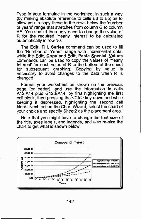
Type in your formulae in the worksheet in such a way(by making absolute reference to cells E3 to E5) as toallow you to copy these in the rows below the 'numberof years' range that stretches from columr G to columnAE. You should then only need to change the value ofR for the required 'Yearly Interest' to be calculatedautomatically in row 10.

The Edit, Fill, Series command can be used to fillthe 'Number of Years' range with incremental data,while the Edit, Copy and Edit, Paste Special, Valuescommands can be used to copy the values of 'YearlyInterest' for each value of R to the bottom of the sheetfor subsequent graphing. Copying by value isnecessary to avoid changes to the data when R ischanged.

Format your worksheet as shown on the previouspage (or better), and use the information in cellsAl2:A14 plus G12:EA14, by first highlighting the firstcell block, then pressing the <Ctrl> key down and whilekeeping it depressed, highlighting the second cellblock. Next, action the Chart Wizard, select the chart ofyour choice and specify Sheet2 as the placement area.

Note that you might have to change the font size ofthe title, axes labels, and legends, and also re -size thechart to get what is shown below.

350710 OD

3:0,1X0 CO

250 0:0 00

t 200=0 CO

0 t 50033 CO

GC 103000 W

50®W

OW

Compound Interest

Years

- Yeah, (L) P-7 50%

-6- Vert, Infirmsi (1) R=1000%

- Yeah/ Interest 0 17).1? 50%

142

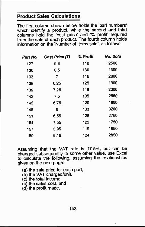
Product Sales Calculations

The first column shown below holds the 'part numbers'which identify a product, while the second and thirdcolumns hold the 'cost price' and '% profit' requiredfrom the sale of eac'i product. The fourth column holdsinformation on the 'Number of items sold', as follows:

Part No. Cost Price (f) % Profit No. Sold

127 5.6 110 2500

130 6.5 130 1300

133 7 115 2800

136 6.25 125 1900

139 7.25 118 2300

142 7.5 135 2550

145 6.75 120 1800

148 E 133 3200

151 6.55 128 2750

154 7.55 122 1750

157 5.95 119 1950

160 6: 6 124 2850

Assuming that the VAT rate is 17.5%, but can bechanged subsequertly to some other value, use Excelto calculate the following, assuming the relationshipsgiven on the next page:

(a) the sale price for each part,(b) the VAT charged/unit,(c) the total income.(c) the sales cost, and(d) the profit made.

143

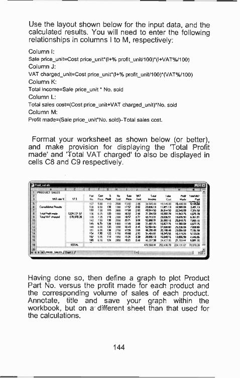
Use the layout shown below for the input data, and thecalculated results. You will need to enter the followingrelationships in columns I to M, respectively:

Column I:Sale pnce_unit=Cost price unit*(1+°/0 profit_unit/100)*(I+VAT%/100)Column J:VAT charged_unit=Cost price_unit*(I+% profit_unit/100)*(VAT%/100)

Column K:Total income=Sale price_unit No. soldColumn L:Total sales cost=(Cost price_unit+VAT charged_unit)*No soldColumn M:Profit made=(Sale price_unit*No. sold) -Total sales cost.

Format your worksheet as shown below (or better),and make provision for displaying the 'Total Profitmade' and 'Total VAT charged' to also be displayed incells C8 and C9 respectively.

1 15106,41 SA1 I S2 Pao Cu 3 No S. 1x6 16161.13 .1 175 No FIN, MW 5120 Po A. Imam Coe 1467 P.1

Ca.4.1.4 R1w4127 563 110 25E0 1162 206 3451503 1914503 1540000 514503130

113

650IL

130

115

130MO

175717 61

262261

22.13611495111

1111 13261.150

10.911500

22540003101137374 50

75,5.ree (22413162lee 136 625 125 1933 1652 26 31 334 03 16 MO 79 14 843 75 4 675 161061VAT (317621 IA 725 111 2360 1657 277 12.71101 230351 1967650 6 SI 51

1 142 750 135 2593 An 301 52.93191 2625016 2511175 766516145 675 120 11130 1745 260 31 637 15 161617 75 1491050 167775141 603 133 3203 16 43 715 37 564 MI 27 02) 03 25 536 03 1 WS 61)151 695 121 2750 1715 261 4625649 251x49 2105610 7 106 99

1 154 7% 122 1750 1569 213 1446411 1034556 11.71923 5 133 061 157 595 119 1950 1571 220 2905613 1601116 1306698 11166E1 160 616 124 29513 1621 241 620712 2147% 21 7s1 44 6661%

t0141 17656144 252.4271 224 101 67 70 978 28 -

as ::11N111106_5411.15 Ow, I / 11t I qr.

Having done so, then define a graph to plot ProductPart No. versus the profit made for each product andthe corresponding volume of sales of each product.Annotate, title and save your graph within theworkbook, but on a different sheet than that used forthe calculations.

144

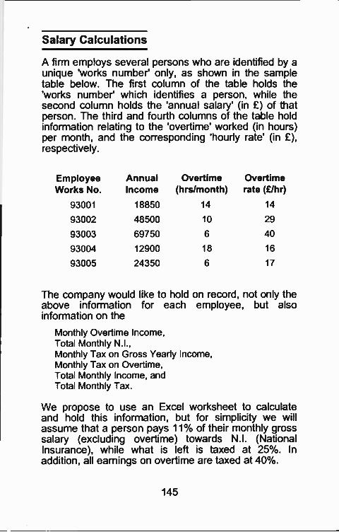
Salary Calculations

A firm employs several persons who are identified by aunique 'works number' only, as shown in the sampletable below. The first column of the table holds the'works number' which identifies a person, while thesecond column holds the 'annual salary' (in £) of thatperson. The third and fourth columns of the table holdinformation relating to the 'overtime' worked (in hours)per month, and the corresponding 'hourly rate' (in £),respectively.

EmployeeWorks No.

AnrualIncome

Overtime(hrs/month)

Overtimerate (£/hr)

93001 16850 14 14

93002 48500 10 29

93003 69750 6 40

93004 12900 18 16

93005 24350 6 17

The company would like to hold on record, not only theabove information for each employee, but alsoinformation on the

Monthly Overtime Income,Total Monthly N.I.,Monthly Tax on Gross Yearly Income,Monthly Tax on Overtime,Total Monthly Income, andTotal Monthly Tax.

We propose to use an Excel worksheet to calculateand hold this information, but for simplicity we willassume that a person pays 11% of their monthly grosssalary (excluding overtime) towards N.I. (NationalInsurance), while what is left is taxed at 25%. Inaddition, all earnings on overtime are taxed at 40%.

145

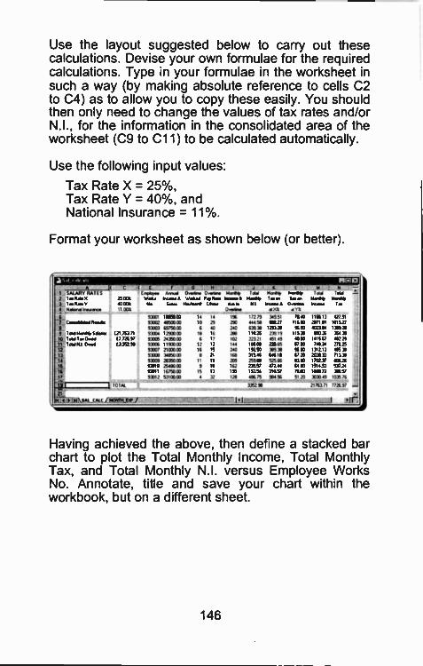
Use the layout suggested below to ca-ry out thesecalculations. Devise your own formulae for the requiredcalculations. Type in your formulae in the worksheet insuch a way (by making absolute reference to cells C2to C4) as to allow you to copy these easily. You shouldthen only need to change the values of tax rates and/orN.I., for the information in the consolidated area of theworksheet (C9 to C11) to be calculated automatically.

Use the following input values:

Tax Rate X = 25%,Tax Rate Y = 40%, andNational Insurance = 11%.

Format your worksheet as shown below (or better).

1 SALARY RAI I52 1aR14%8 la Ram Y

14414.54 Inwmarea

CANNAL4 Re..

9 1NA Mont* 51168e.10 laug 1=044.11 10 76% 04441213

11

141617

I

25 31240001

E

(now.Work,

Ne

844 6.........imam Waits

Ga. KO,. ,

31

0 wormP. RAMLAN,

Mai"Ircom 8Jets

4CI411

Med*1/ 1

144n1Ny

wawa 6

I.RN.,lam

0 AAA.

14

10dNard4,Year

NIllNed;

IN1103* 04411. 4191 4'04

43101 18E60 14 14 1% 172 79 34951 1940 11%12 42191UN 44503 I0 29 NO 44458 999.27 11632 2971 111 10152793023 123793 6 10 240 639 311 1 293 28 X00 4023 IN 1319 21

121 163 11 93334 12903 16 16 208 111125 23919 115 20 NON 151 39I 7 726 97 93305 24350 6 17 102 27321 45149 40 10 1415 67 49229I 3 152 96 NON 11900 12 12 144 10960 22065 5760 11934 27625

91137 21011 16 15 240 19250 797 9600 131213 485 3893333 34850 8 7 IN 319 46 61619 6120 20733 713 3391009 28350 II 19 NO 29971 52516 ealia 170237 609 2693010 25420 9 II 162 23357 472 44 6410 1514 53 537 24

mmi 16750 15 13 195 153 54 31057 7109 101 72 344 51

93012 51100 4 32 128 446 75 984 % 51 20 7719 1 OM 76

10140 315291 21 NJ 71 71X91

11'.14\sujut wimp, / 11 I.11:

Having achieved the above, then define a stacked barchart to plot the Total Monthly Income, Total MonthlyTax, and Total Monthly N.I. versus Employee WorksNo. Annotate, title and save your chart within theworkbook, but on a different sheet.

146

10. FUNCTIONS

Excel's functions are built-in formulae that performspecialised calculations. Their general format is:

name(arg1,arg2,...)

where 'name' is the function name, and 'arg1', 'arg2',etc., are the arguments required for the evaluation ofthe function. Arguments must appear in a

parenthesized list as shown above and their exactnumber depends on the function being used. However,some functions do not require arguments and are usedwithout parentheses. Examples of these are: FALSE,NA, NOW, PI, RAND, TODAY and TRUE.

There are four :ypes of arguments used withfunctions: numeric values, range values, string va uesand conditions, the type used being dependent on thetype of function. Numeric value arguments can beentered either directly as numbers, as a cell address, acell range name or as a formula. Range valuearguments can be entered either as a range address ora range name, while string value arguments car beentered as an actual value (a string in double quotes),as a cell address, a cell name, or a formula. Cond tionarguments normally use logical operators or refer to anaddress containing a logic formula.

Types of Functions

There are several types of functions in Excel 97,namely, financial, date and time, mathematical andtrigonometric, statistical, lookup and reference,database, text, logical, and information. Each type offunction requires its own number and type ofarguments. These are listed on the next few pagesunder the various function categories. To find out indetail how these functions can be used, click the EditFormula button (*) to display:

147

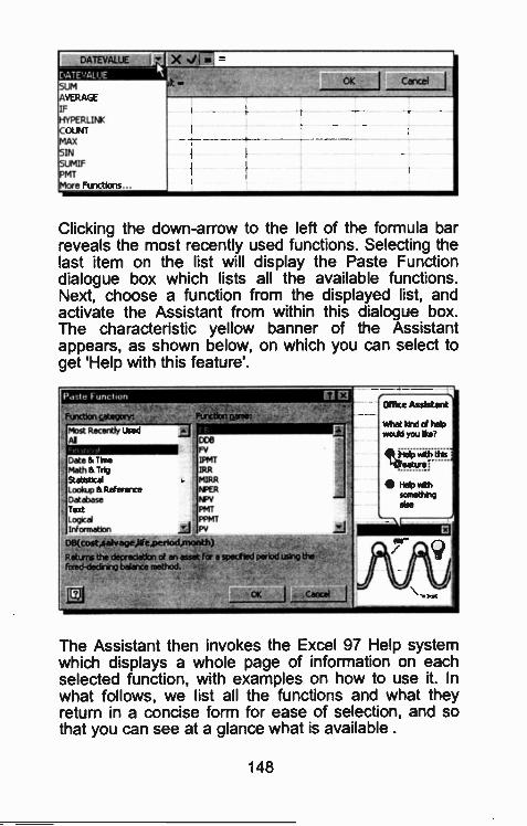
DATEVALUE Lj x =

SUMAVERAGE

IFHYPERLIWCOUNTMAX

SINSUMIFPMT

Mae Functions...

OK I Cancel

Clicking the down-arrow to the left of the formula barreveals the most recently used functions. Selecting thelast item on the list will display the Paste Functiondialogue box which lists all the available functions.Next, choose a function from the displayed list, andactivate the Assistant from within this dialogue box.The characteristic yellow banner of the Assistantappears, as shown below, on which you can select toget 'Help with this feature'.

CatigarY1

Most Recently UsedDCO

. FV

Date & Trne IPMT

Math & Trio IRR

Statistical MIRRLook & Reference NFfRDatabase WYText PMT

Lewd PPMT

Information PV

DIXcost,satvageAte,period,rnonth)Returns the depreciation of an for # sr,tied perioducrc.feted -clacking baLsnce methcid.,

The Assistant then invokes the Excel 97 Help systemwhich displays a whole page of information on eachselected function, with examples on how to use it. Inwhat follows, we list all the functions and what theyreturn in a concise form for ease of selection, and sothat you can see at a glance what is available .

148

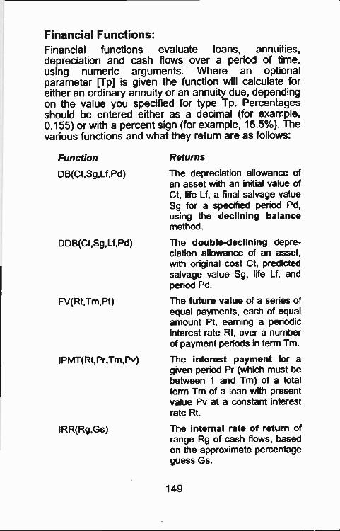
Financial Functions:Financial functions evaluate loans, annuities,depreciation and cash flows over a period of time,using numeric arguments. Where an optionalparameter [Tp] is given the function will calculate foreither an ordinary annuity or an annuity due, dependingon the value you specified for type Tp. Percentagesshould be entered either as a decimal (for exarrple,0.155) or with a percent sign (for example, 15.5%). Thevarious functions and what they return are as follows:

Function Returns

DB(Ct,Sg,Lf,Pd) The depreciation allowance ofan asset with an initial value ofCt, life Lf, a final salvage valueSg for a specified period Pd,using the declining balancemethod.

DDB(Ct,Sg,Lf,Pd) The double -declining depre-ciation allowance of an asset,with original cost Ct, predictedsalvage value Sg, li'e Lf, andperiod Pd.

FV(Rt,Tm,Pt) The future value of a series ofequal payments, each of equalamount Pt, earning a periodicinterest rate Rt, over a numberof payment periods in term Tm.

IPMT(Rt,Pr,Tm,Pv) The interest payment for agiven period Pr (which must bebetween 1 and Tm) of a totalterm Tm of a loan with presentvalue Pv at a constant interestrate Rt.

IRR(Rg,Gs) The internal rate of return ofrange Rg of cash flows, basedon the approximate percentageguess Gs.

149

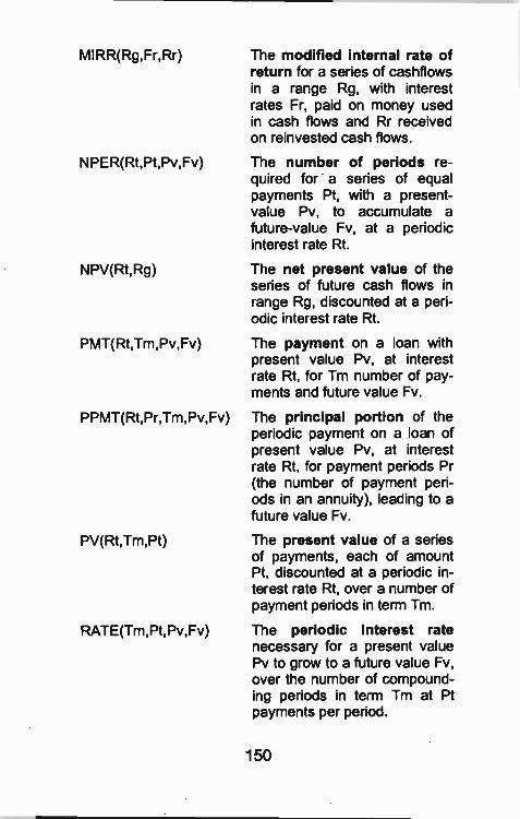
MIRR(Rg,Fr,Rr)

NPER(Rt,Pt,Pv,Fv)

NPV(Rt,Rg)

PMT(Rt,Tm,Pv,Fv)

The modified internal rate ofreturn for a series of cashflowsin a range Rg, with interestrates Fr, paid on money usedin cash flows and Rr receivedon reinvested cash flows.

The number of periods re-quired for a series of equalpayments Pt, with a present -value Pv, to accumulate a

future -value Fv, at a periodicinterest rate Rt.

The net present value of theseries of future cash flows inrange Rg, discounted at a peri-odic interest rate Rt.

The payment on a loan withpresent value Pv, at interestrate Rt, for Tm number of pay-ments and future value Fv.

PPMT(Rt,Pr,Tm,Pv,Fv) The principal portion of theperiodic payment on a loan ofpresent value Pv, at interestrate Rt, for payment periods Pr(the number of payment peri-ods in an annuity), leading to afuture value Fv.

PV(Rt,Tm,Pt) The present value of a seriesof payments, each of amountPt, discounted at a periodic in-terest rate Rt, over a number ofpayment periods in term Tm.

RATE(Tm,Pt,Pv,Fv) The periodic interest ratenecessary for a present valuePv to grow to a future value Fv,over the number of compound-ing periods in term Tm at Ptpayments per period.

150

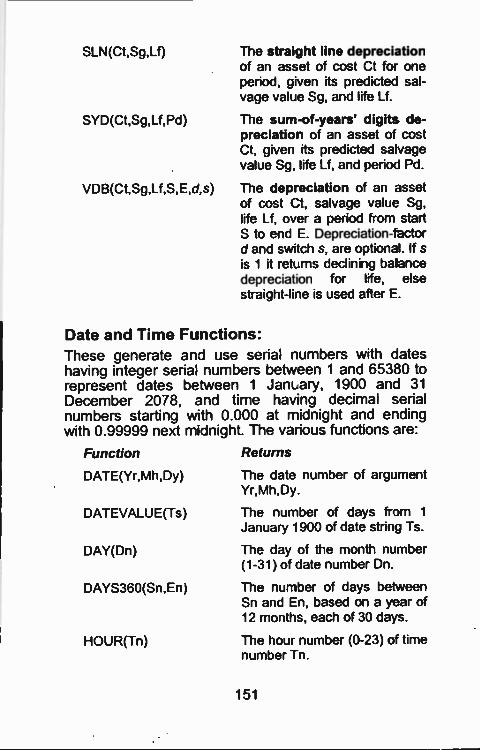
SLN(Ct,Sg,Lf) The straight line depreciationof an asset of cost Ct for oneperiod, given its predicted sal-vage value Sg, and life Lf.

SYD(Ct,Sg,Lf,Pd) The sum -of -years' digits de-preciation of an asset of costCt, given its predicted salvagevalue Sg, rife Lf, and perioa Pd.

VDB(Ct,Sg,Lf,S,E.d s) The depreciation of an assetof cost Ct, salvage value Sg,life Lf, over a period from startS to end E. Depreciation -factord and switch s, are optional. If sis 1 it retuns declining balancedepreciation for life, elsestraight-line is used after E.

Date and Time Functions:These generate and use serial numbers with dateshaving integer serial numbersrepresent dates between 1 January, 1900 and 31December 2078, and time having decimal serialnumbers starting with 0.000 at midnight and endingwith 0.99999 next midnight. The various functions are:

Function Returns

DATE (Yr,M h ,Dy)

DATEVALUE(Ts;

DAY(Dn)

DAYS360(Sn,En)

HOUR(Tn)

The date number of argumentYr,Mh,Dy.

The number of days from 1

January 1900 of date string Ts.

The day of the month number(1-31) of date number Dn.

The number of days betweenSn and En, based on a year of12 months, each of 30 dais.

The hour number (0-23) of timenumber Tn.

151

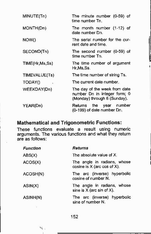
MINUTE(Tn)

MONTH(Dn)

NOW()

SECOND(Tn)

TIME(Hr,Ms,Ss)

The minute number (0-59) oftime number Tn.

The month number (1-12) ofdate number Dn.

The serial number for the cur-rent date and time.

The second number (0-59) oftime number Tn.

The time number of argumentHr,Ms,Ss.

TIMEVALUE(Ts) The time number of string Ts.

TODAY() The current date number.

WEEKDAY(Dn) The day of the week from datenumber Dn in in-.eger form; 0(Monday) through 6 (Sunday).

YEAR(Dn) Returns the year number(0-199) of date number Dn.

Mathematical and Trigonometric Functions:These functions evaluate a result using numericarguments. The various functions and wha-. they returnare as follows:

Function Returns

ABS(X) The absolute value of X.

ACOS(X) The angle in radians, whosecosine is X (arc cos of X).

ACOSH(N) The arc (inverse) hyperboliccosine of number N.

ASIN(X) The angle in radians, whosesine is X (arc sin o' X).

ASINH(N) The arc (inverse) hyperbolicsine of number N.

152

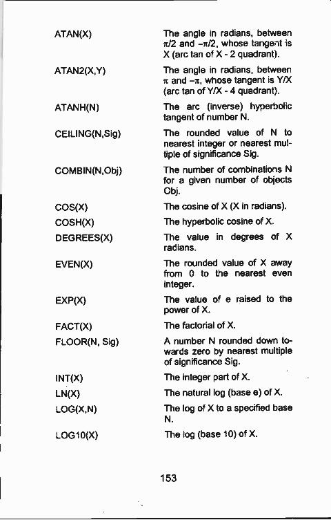
ATAN(X) The angle in radians, behkeenm/2 and -n/2, whose tangent isX (arc tan of X - 2 quadrant).

ATAN2(X,Y) The angle in radians, betweenit and -7I, whose tangent is Y/X(arc tan of Y/X - 4 quadrant).

ATANH(N) The arc (inverse) hyperbolictangent of number N.

CEILING(N,Sig) The rounded value of N tonearest in:eger or nearest mul-tiple of significance Sig.

COMBIN(N,Obj) The number of combinatiols Nfor a given number of objectsObj.

COS(X) The cosine of X (X in radials).

COSH(X) The hyperbolic cosine of X.

DEGREES(X) The value in degrees of Xradians.

EVEN(X) The rounded value of X awayfrom 0 to the nearest eveninteger.

EXP(X) The value of e raised to thepower of X.

FACT(X) The factorial of X.

FLOOR(N, Sig) A number N rounded down to-wards zero by nearest multipleof significance Sig.

INT(X) The integer part of X.

LN(X) The natu-al log (base e) of X.

LOG(X,N) The log of X to a specified baseN.

LOG10(X) The log (base 10) of X.

153

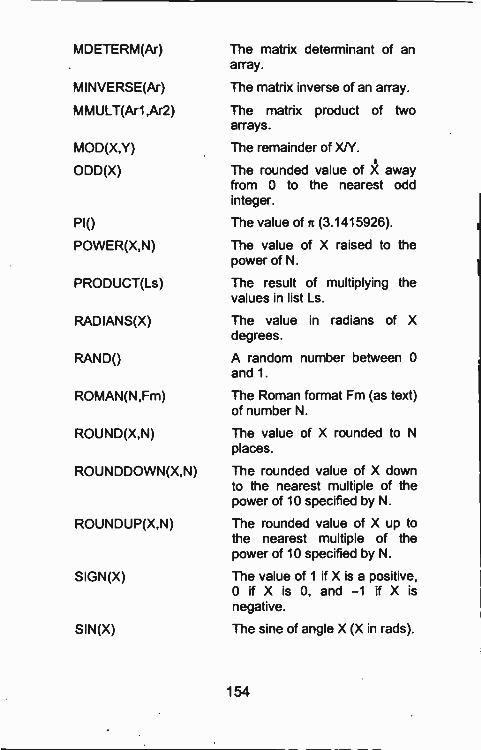
MDETERM(Ar) The matrix deteminant of anarray.

MINVERSE(Ar) The matrix inverse of an array.

MMULT(Ar1,Ar2) The matrix prcduct of twoarrays.

MOD(X,Y) The remainder of XJY.

ODD(X) The rounded value of X awayfrom 0 to the nearest oddinteger.

PI() The value of is (3.1415926).

POWER(X,N) The value of X raised to thepower of N.

PRODUCT(Ls) The result of multiplying thevalues in list Ls.

RADIANS(X) The value in radians of Xdegrees.

RAND() A random number between 0and 1.

ROMAN(N,Fm) The Roman format Fm (as text)of number N.

ROUND(X,N) The value of X rounded to Nplaces.

ROUNDDOWN(X,N) The rounded value of X downto the nearest multiple of thepower of 10 specified by N.

ROUNDUP(X,N) The rounded value of X up tothe nearest multiple of thepower of 10 specified by N.

SIGN(X) The value of 1 if X is a positive,0 if X is 0, and -1 if X isnegative.

SIN(X) The sine of angle X (X in rads).

154

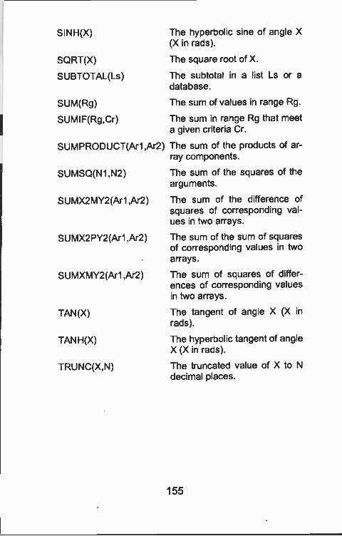
SINH(X)

SQRT(X)

SUBTOTAL(Ls)

SUM(Rg)

SUMIF(Rg,Cr)

SUMPRODUCT(Ar1,Ar2)

SUMSQ(N1,N2)

SUMX2MY2(Ar1,Ar2)

SUMX2PY2(Ar1,Ar2)

SUMXMY2(Ar1,Ar2)

TAN(X)

TANH(X)

TRUNC(X,N)

The hyperbolic sine cf angle X(X in rads)

The square root of X.

The subtotal in a is: Ls or adatabase.

The sum of values in range Rg.

The sum in range Rg that meeta given criteria Cr.

The sum of the products of ar-ray components.

The sum of the squares of thearguments.

The sum of the difference ofsquares of corresponding val-ues in two arrays.

The sum of the sum of squaresof corresponding values in twoarrays.

The sum of squares of differ-ences of corresponding valuesin two arrays.

The tangent of angle X (X inrads).

The hyperoolic tangent of angleX (X in rats).

The truncated value of X to Ndecimal places.

155

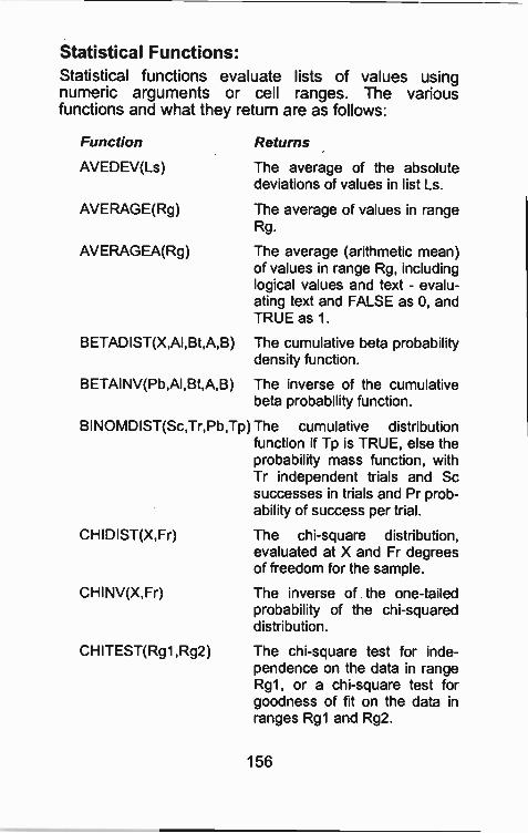
Statistical Functions:Statistical functions evaluate lists of values usingnumeric arguments or cell ranges. The variousfunctions and what they return are as follows:

Function Returns

AVEDEV(Ls) The average of the absolutedeviations of values in list Ls.

AVERAGE(Rg) The average of values in rangeRg.

AVERAGEA(Rg) The average (arithmetic mean)of values in range Rg, includinglogical values and text - evalu-ating text and FALSE as 0, andTRUE as 1.

BETADIST(X,AI,Bt,A,B) The cumulative beta probabilitydensity function.

BETAINV(Pb,AI,Bt,A,B) The inverse of the cumulativebeta probability function.

BINOMDIST(Sc,Tr,Pb,Tp) The cumulative distributionfunction if Tp is TRUE, else theprobability mass function, withTr independent trials and Scsuccesses in trials and Pr prob-ability of success per trial.

CHIDIST(X, Fr) The chi-square distribution,evaluated at X and Fr degreesof freedom for the sample.

CHINV(X,Fr) The inverse of the one -tailedprobability of the chi -squareddistribution.

CHITEST(Rg1,Rg2) The chi-square test for inde-pendence on the data in rangeRg1, or a chi-square test forgoodness of fit on the data inranges Rg1 and Rg2.

156

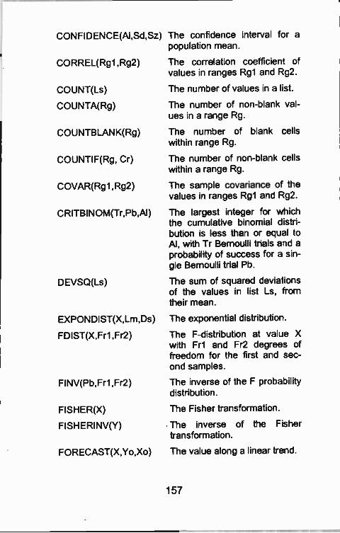
CONFIDENCE(AI,Sd,Sz)

CORREL(Rgl ,Rg2)

COUNT(Ls)

COUNTA(Rg)

COUNTBLANK(Rg)

COUNTIF(Rg, Cr)

COVAR(Rgl ,Rg2)

CRITBINOM(Tr,Pb,AI)

DEVSQ(Ls)

EXPONDIST(X,Lm,Ds)

FDIST(X,Frl ,Fr2)

FINV(Pb,Frl ,Fr2)

FISHER(X)

FISHERINV(Y)

FORECAST(X,Yo,Xo)

The confidence interval for apopulation mean.

The correlation coefficient ofvalues in ranges Rgl and Rg2.

The number of values in a I st.

The number of non -blank val-ues in a range Rg.

The number of blank cellswithin ranee Rg.

The number of non -blank cellswithin a range Rg.

The sample covariance of thevalues in ranges Rgl and Rg2.

The largest integer for whichthe cumulative binomial distri-bution is less than or equal toAI, with Tr Bernoulli trials aid aprobability of success for a sin-gle Bernoulli trial Pb.

The sum of squared deviationsof the values in list Ls, fromtheir mean.

The exponential distributior.

The F -distribution at value Xwith Fri and Fr2 degrees offreedom for the first and sec-ond samples.

The inverse of the F probabilitydistribution.

The Fisher transformation.

The inverse of the Fishertransformation.

The value along a linear trend.

157

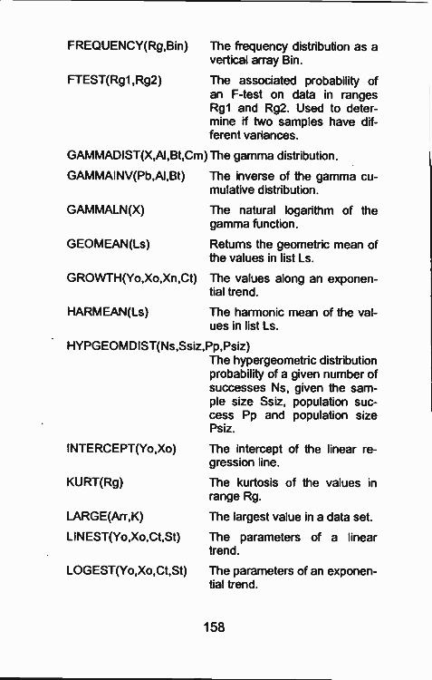
FREQUENCY(Rg,Bin)

FTEST(Rgl,Rg2)

The frequency distribution as avertical array Bin.

The associated probability ofan F -test on data in rangesRgl and Rg2. Used to deter-mine if two samples have dif-ferent variances.

GAMMADIST(X,AI,Bt,Cm) The gamma distribution.

GAMMAINV(Pb,AI,Bt) The inverse of the gamma cu-mulative distribution.

GAMMALN(X) The natural logarithm of thegamma function.

GEOMEAN(Ls) Returns the geometric mean ofthe values in list Ls.

GROWTH(Yo,Xo,Xn,Ct) The values along an exponen-tial trend.

HARMEAN(Ls) The harmonic mean of the val-ues in list Ls.

HYPGEOMDIST(Ns,Ssiz,Pp,Psiz)The hypergeometric distributionprobability of a given number ofsuccesses Ns, given the sam-ple size Ssiz, population suc-cess Pp and population sizePsiz.

INTERCEPT(Yo,Xo) The intercept of the linear re-gression line.

KURT(Rg) The kurtosis of the values inrange Rg.

LARGE(Arr,K)

LINEST(Yo,Xo,Ct,St)

LOGEST(Yo,Xo,Ct,St)

The largest value in a data set.

The parameters of a lineartrend.

The parameters of an exponen-tial trend.

158

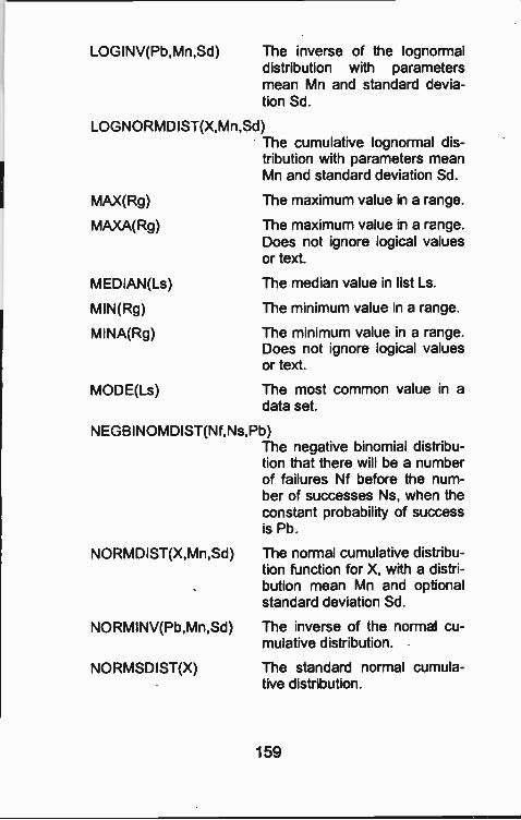
LOGINV(Pb,Mn,Sd) The inverse of the logncrmaldistribution with parametersmean Mn and standard devia-tion Sd.

LOGNORMDIST(X,Mn,Sd)The cumulative lognormal dis-tribution with parameters meanMn and standard dev ation Sd.

MAX(Rg) The maximum value in a range.

MAXA(Rg) The maximum value in a range.Does not ignore logical valuesor text.

MEDIAN(Ls) The median value in list Ls

MIN(Rg) The minimum value in a range.

MINA(Rg) The minimum value '1 a range.Does not ignore logical valuesor text.

MODE(Ls) The most common value in adata set.

NEGBINOMDIST(Nf,Ns,Pb)

NORMDIST(X,Mn,Sd)

The nega*.ive binomial distribu-tion that there will be a numberof failures Nf before the num-ber of successes Ns, when theconstant probability of successis Pb.

The normal cumulative distribu-tion function for X, with a distri-bution mean Mn and optionalstandard deviation Sd.

NORMINV(Pb,Mn,Sd) The inverse of the normal cu-mulative distribution.

NORMSDIST(X) The standard normal cumula-tive distribution.

159

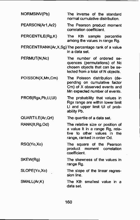
NORMSINV(Pb) The inverse of the standardnormal cumulative distribution.

PEARSON(Arl ,Ar2) The Pearson product momentcorrelation coefficient.

PERCENTILE(Rg,K) The Kth sample percentileamong the values in range Rg.

PERCENTRANK(Ar,X,Sg)The percentage rank of a valuein a data set.

PERMUT(N,Nc)

POISSON(X,Mn,Cm)

PROB(Rgx,Pb,LI,U1)

QUARTILE(Ar,Qrt)

RANK(It,Rg,0d)

RSQ(Yo,Xo)

The number of ordered se-quences (permutations) of Ncchosen objects that can be se-lected from a total of N objects.

The Poisson distribution (de-pending on cumulative factorCm) of X observed events andMn expected number of events.

The probability that values inRgx range are within lower limitLI and upper limit UI of prob-ability Pb.

The quartile of a data set.

The relative size or position ofa value It in a range Rg, rela-tive to other values in therange, ranked in order Od.

The square of the Pearsonproduct momert correlationcoefficient.

SKEW(Rg) The skewness of the values inrange Rg.

SLOPE(Yo,Xo) The slope of the linear regres-sion line.

SMALL(Ar,K) The Kth smallest value in adata set.

160

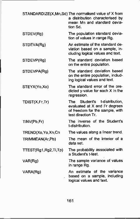
STANDARDIZE(X,Mn,Sd) The normalised value of X froma distribution characterised bymean Mn and standard devia-tion Sd.

STDEV(Rg)

STDEVA(Rg)

STDEVP(Rg)

STDEVPA(Rg)

STEYX(Yo,Xo)

TDIST(X,Fr,Tr)

The population standard devia-tion of values in range Rg.

An estimate of the standard de-viation based on a sample, in-cluding logical values and text.

The standard deviation basedon the entire population.

The standard deviation basedon the entire population, includ-ing logical values and text.

The standard error of the ore-dicted y -value for each X in theregression.

The Stucent's t -distribution,evaluated at X and Fr degreesof freedom for the sample, withtest direction Tr.

TINV(Pb,Fr) The inverse of the Student'st -distribution.

TREND(Xo,Yo,Xn,C1

TRIMMEAN(Ar,Pb)

The values along a linear trend.

The mean of the interior of adata set.

TTEST(Rg1,Rg2,TI,Tp) The probability associated witha Student's t -test.

VAR(Rg) The sample variance of valuesin range Rg.

VARA(Rg) An estimate of the variancebased on a sample, includinglogical values and text.

161

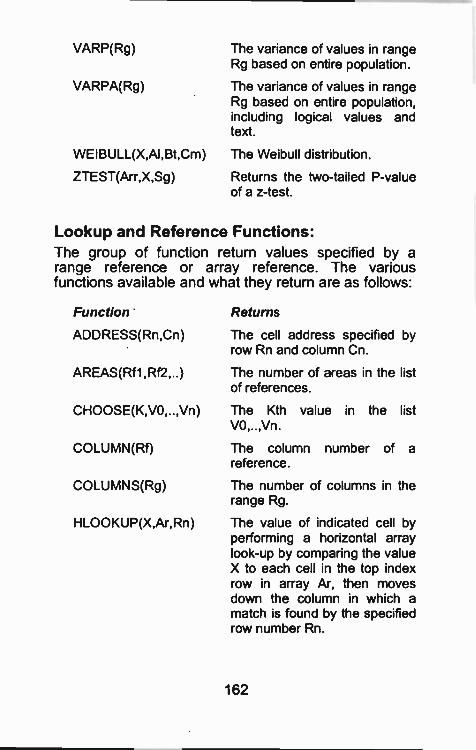
VARP(Rg) The variance of values in rangeRg based on entire population.

VARPA(Rg) The variance of values in rangeRg based on entire population,including logical values andtext.

WEIBULL(X,AI,Bt,Cm)

ZTEST(Arr,X,Sg)

The Weibull distribution.

Returns the two -tailed P -valueof a z -test.

Lookup and Reference Functions:The group of function return values specified by arange reference or array reference. The variousfunctions available and what they return are as follows:

Function Returns

ADDRESS(Rn,Cn) The cell address specified byrow Rn and column Cn.

AREAS(Rfl,Rf2,..) The number of areas in the listof references.

CHOOSE(K,VO,..,Vn) The Kth value in the listVO,..,Vn.

COLUMN(Rf) The column number of areference.

COLUMNS(Rg) The number of columns in therange Rg.

HLOOKUP(X,Ar,Rn) The value of incicated cell byperforming a horizontal arraylook -up by comparing the valueX to each cell in the top indexrow in array Ar then movesdown the column in which amatch is found by the specifiedrow number Rn.

162

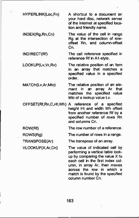
HYPERLINK(Loc,Fn) A shortcut to a document onyour hard disc, network serverof the Internet at specified loca-tion and friendly name.

INDEX(Rg,Rn,Cn) The value of the cell in rangeRg at the intersection of row -offset Rn, and column -offsetCn.

INDIRECT(Rf) The cell reference specified inreference Rf in Al -style.

LOOKUP(Lv,Vr,Rv) The relative position of an ternin an array that matches aspecified value in a specifiedorder.

MATCH(Lv,Ar,Mtc) The relative position of an ele-ment in an array Ar thatmatches the specified valueMtc of a lookup value Lv.

OFFSET(Rf,Rn,C,rit,Wh) A reference of a specifiedheight Ht and width Wh offsetfrom another reference Rf oy aspecified lumber of rows Rnand columns Cn.

ROW(Rf) The row number of a -eference.

ROWS(Rg) The number of rows in a ra-ige.

TRANSPOSE(Ar) The transpose of an array.

VLOOKUP(X,Ar,Cn, The value of indicated cell byperforming a vertical table look-up by comparing the value X toeach cell in the first index col-umn, in array Ar, then movesacross the row in which a

match is found by the specifiedcolumn number Cn.

163

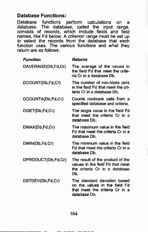
Database Functions:Database functions perform calculations on adatabase. The database, called the input range,consists of records, which include fie'ds and fieldnames, like Fd below. A criterion range must be set upto select the records from the database that eachfunction uses. The various functions and what theyreturn are as follows:

Function Returns

DAVERAGE(Db,Fd,Cr) The average of the values inthe field Fd that meet the crite-ria Cr in a database Db.

DCOUNT(Db,Fd,Cr) The number of non -blank cellsin the field Fd that meet the cri-teria Cr in a database Db.

DCOUNTA(Db,Fd,Cr) Counts nonblank cells from aspecified database and criteria.

DGET(Db,Fd,Cr) The single value in the field Fdthat meet the criteria Cr in adatabase Db.

DMAX(Db,Fd,Cr) The maximum value in the fieldFd that meet the criteria Cr in adatabase Db.

DMIN(Db,Fd,Cr) The minimum va ue in the fieldFd that meet the criteria Cr in adatabase Db.

DPRODUCT(Db,Fd,Cr) The result of the product of thevalues in the field Fd that meetthe criteria Cr in a databaseDb.

DSTDEV(Db,Fd,Cr) The standard deviation basedon the values in the field Fdthat meet the criteria Cr in adatabase Db.

164

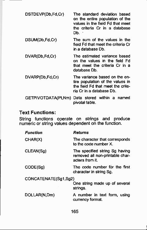
DSTDEVP(Db,Fd,Cr)

DSUM(Db,Fd,Cr)

DVAR(Db,Fd,Cr)

DVARP(Db,Fd,Cr)

The standard deviation basedon the entire population of thevalues in tie field Fd that meetthe criteria Cr in a databaseDb.

The sum of the values in thefield Fd that meet the criteria Crin a database Db.

The estimated variance basedon the values in the field Fdthat meet the criteria Cr in adatabase Db.

The variance based on the en-tire population of the values inthe field Fd that meet the crite-ria Cr in a database Db.

GETPIVOTDATA.;Pt,Nm) Data stored within a namedpivotal table.

Text Functions:String functions operate on strings and producenumeric or string values dependent on the function.

Function Returns

CHAR(X) The character that correspondsto the code number X.

CLEAN(Sg) The specified string Sg havingremoved all non -printable char-acters from it.

CODE(Sg) The code number for the firstcharacte- in string Sg.

CONCATENATE(Sgl ,Sg2)One string made up of severalstrings.

DOLLAR(N,Dm) A number in text form, usingcurrency format.

165

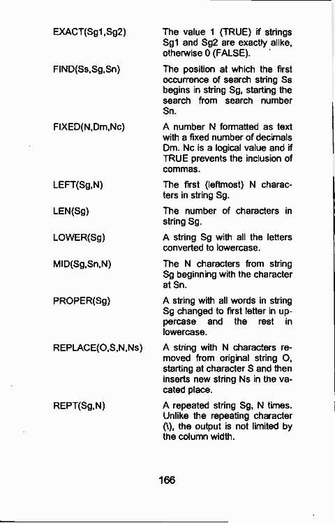
EXACT(Sg 1 ,Sg2) The value 1 (TRUE) if stringsSgt and Sg2 are exactly alike,otherwise 0 (FALSE).

FIND(Ss,Sg,Sn) The position at which the firstoccurrence of search string Ssbegins in string Sg, starting thesearch from search numberSn.

FIXED(N,Dm,Nc) A number N formatted as textwith a fixed number of decimalsDm. Nc is a logical value and ifTRUE prevents the inclusion ofcommas.

LEFT(Sg,N) The first (leftmost) N charac-ters in string Sg.

LEN(Sg) The number of characters in

string Sg.

LOWER(Sg) A string Sg with all the lettersconverted to lowercase.

MID(Sg,Sn,N) The N characters from stringSg beginning with the characterat Sn.

PROPER(Sg)

REPLACE(0,S,N,Ns)

REPT(Sg,N)

A string with all words in stringSg changed to first letter in up-percase and the rest in

lowercase.

A string with N characters re-moved from original string 0,starting at character S and theninserts new string Ns in the va-cated place.

A repeated string Sg, N times.Unlike the repeating character(\), the output is rot limited bythe column width.

166

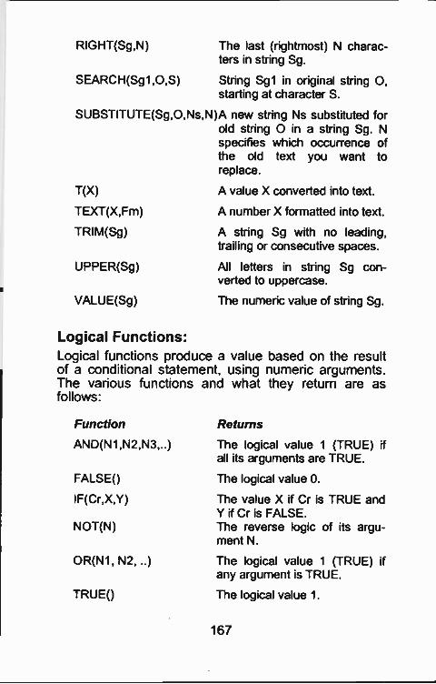
RIGHT(Sg,N) The last (rightmost) N charac-ters in string Sg.

SEARCH(Sg1,0,S) String Sgt in original string 0,starting at character S.

SUBSTITUTE(Sg,O,Ns,N)A new string Ns substituted forold string 0 in a string Sg. Nspecifies which occurrence ofthe old text you wan: toreplace.

T(X) A value X converted into text.

TEXT(X,Fm) A number X formatted into text.

TRIM(Sg) A string Sg with no leading,trailing or consecutive spaces.

UPPER(Sg) All letters in string Sg con-verted to uppercase.

VALUE(Sg) The numeric value of string Sg.

Logical Functions:Logical functions produce a value based on the resultof a conditional statement, using numeric arguments.The various functions and what they return are, asfollows:

Function Returns

AND(N1,N2,N3,..) The logical value 1 (TRUE) ifall its arguments are TRUE.

FALSE() The logical value 0.

IF(Cr,X,Y) The value X if Cr is TRUE andY if Cr is FALSE.

NOT(N) The reverse logic of its argu-ment N.

OR(N1, N2, ..) The logical value 1 (TRJE) ifany argument is TRUE.

TRUE() The logical value 1.

167

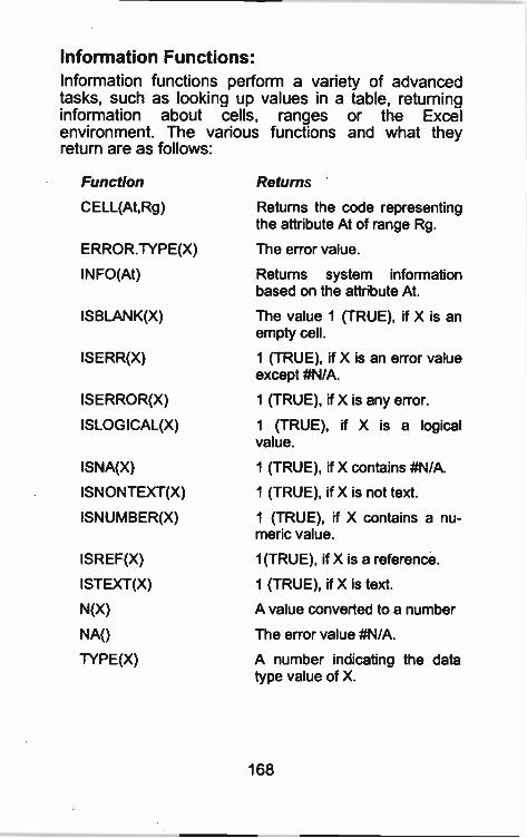
Information Functions:Information functions perform a variety of advancedtasks, such as looking up values in a table, returninginformation about cells, ranges or the Excelenvironment. The various functions and what theyreturn are as follows:

Function Returns

CELL(At,Rg) Returns the code representingthe attribute At of range Rg.

ERROR.TYPE(X) The error value.

INFO(At) Returns system informationbased on the attr bute At.

ISBLANK(X) The value 1 (TRUE), if X is anempty cell.

ISERR(X) 1 (TRUE), if X is an error valueexcept #N/A.

ISERROR(X) 1 (TRUE), if X is any error.

ISLOGICAL(X) 1 (TRUE), if X is a logicalvalue.

ISNA(X) 1 (TRUE), if X contains #N/A.

ISNONTEXT(X) 1 (TRUE), if X is not text.

ISNUMBER(X) 1 (TRUE), if X contains a nu-meric value.

ISREF(X) 1(TRUE), if X is a reference.

ISTEXT(X) 1 (TRUE), if X is text.

N(X) A value converted to a number

NA() The error value #N/A.

TYPE(X) A number indicating the datatype value of X.

168

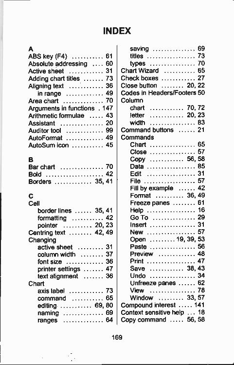
INDEX

AABS key (F4) 61

Absolute addressing 60Active sheet 31

Adding chart titles 73Aligning text 36

in range 49Area chart 70Arguments in functions 147Arithmetic formulae 43Assistant 20Auditor tool 99AutoFormat 49AutoSum icon 45

BBar chart 70Bold 42Borders 35, 41

CCell

border lines 35, 41formatting 42pointer 20, 23

Centring text 42, 49Changing

active sheet 31

column width 37font size 36printer settings 47text alignment 36

Chartaxis label 73command 65editing 69, 80naming 69ranges 64

saving 69titles 73types 70

Chart Wizard 65Check boxes 27Close button 20 22Codes in Headers/Footers 50Column

chart 70, 72letter 20, 23width 83

Commard buttons 21

CommandsChart 65Close 57Copy 56, 58Data 85Edit 31

File 57Fill by example 42Format 36, 49Freeze panes 61

Help 16Go To 29Insert 31

New 57Open 19, 39, 53Paste 56Prey ew 48Print 47Save 38, 43Undo 34Unfreeze panes 62View 78Window 33, 57

Compound interest 141

Context sensitive help . . 18Copy command 56, 58

169

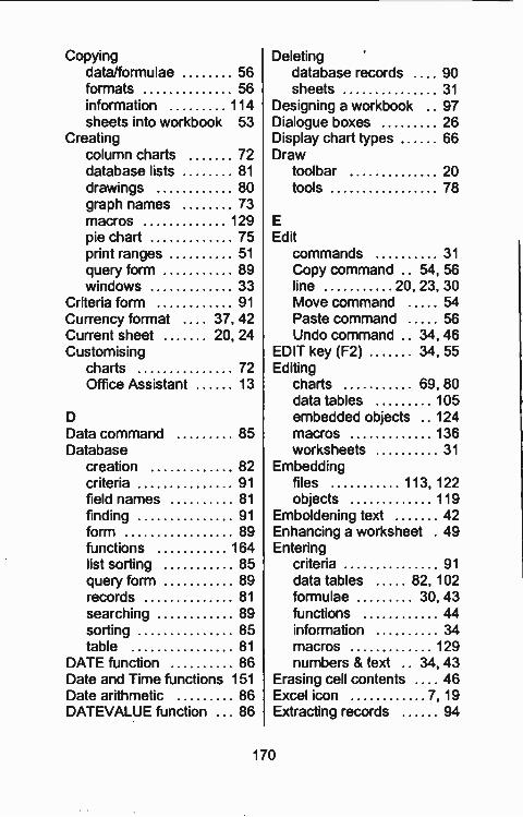
Copyingdata/formulae 56formats 56information 114sheets into workbook 53

Creatingcolumn chartsdatabase listsdrawingsgraph namesmacrospie chartprint rangesquery form 89windows 33

Criteria form 91

7281

8073

1297551

Currency format 37, 42Current sheet 20, 24Customising

charts 72Office Assistant 13

DData command 85Database

creation 82criteria 91field names 81

finding 91form 89functions 164list sorting 85query form 89records 81

searching 89sorting 85table 81

DATE function 86Date and Time functions 151Date arithmetic 86DATEVALUE function 86

Deletingdatabase records 90sheets 31

Designing a workbook 97Dialogue boxes 26Display chart types 66Draw

toolbar 20tools 78

EEdit

commands 31

Copy command .. 54, 56line 20, 23, 30Move command 54Paste command 56Undo command . 34, 46

EDIT key (F2) 34, 55Editing

charts 69, 80data tables 105embedded objects 124macros 136worksheets 31

Embeddingfiles 113, 122objects 119

Emboldening text 42Enhancing a worksheet 49Entering

criteria 91

data tables 82, 102formulae 30, 43functions 44information 34macros 129numbers & text .. 34, 43

Erasing cell contents .... 46Excel icon 7, 19Extracting records 94

170

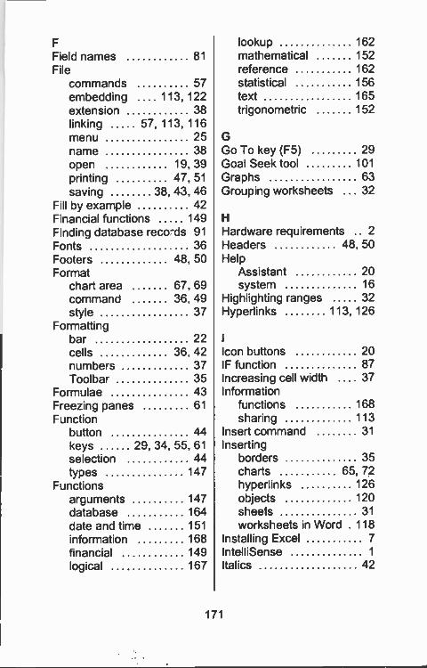
F

Field names 81

Filecommands 57embedding .... 113, 122extension 38linking 57, 113, 116menu 25name 38open 19, 39printing 47, 51saving 38, 43, 46

Fill by example ...... 42Financial functions .. .. 149Finding database reco-ds 91Fonts 36Footers 48, 50Format

chart area 67, 69command 36, 49style 37

Formattingbar 22cells 36, 42numbers 37Toolbar 35

Formulae 43Freezing panes 61

Functionbutton 44keys 29, 34 55, 61selection 44types 147

Functionsarguments 147database 164date and time 151

information 168financial 149logical 167

171

lookup 162mathematical 152reference .. 162statistical 156text 165trigonometric 152

GGo To key (F5) 29Goal Seek tool 101

Graphs 63Grouping worksheets 32

HHardware requirements .. 2

Headers 48, 50Help

Assis*.ant 20system 16

Highlighting ranges 32Hyperlinks 113, 126

Icon buttons 20IF function 87Increasing cell widtt 37Information

functions 168sharing 113

Insert command 31

Insertingborders 35charts 65, 72hyperlinks 126objects 120sheets 31

worksheets in Word 118Installing Excel 7

IntelliSense 1

Italics 42

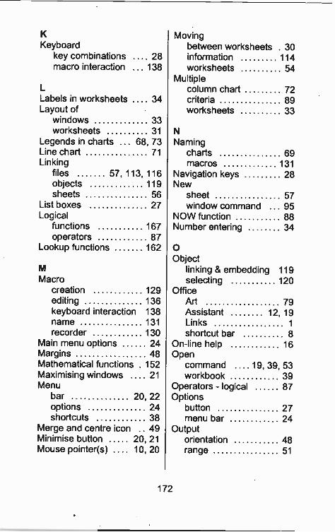
KKeyboard

key combinations .... 28macro interaction ... 138

LLabels in worksheets .... 34Layout of

windows 33worksheets 31

Legends in charts ... 68, 73Line chart 71Linking

files 57, 113, 116objects 119sheets 56

List boxes 27Logical

functions 167operators 87

Lookup functions 162

M

Macrocreation 129editing 136keyboard interaction 138name 131recorder 130

Main menu options 24Margins 48Mathematical functions . 152Maximising windows 21Menu

bar 20, 22options 24shortcuts 38

Merge and centre icon 49Minimise button 20, 21Mouse pointer(s) 10, 20

Movingbetween worksheets . 30information 114worksheets 54

Multiplecolumn chart 72criteria 89worksheets 33

N

Namingcharts 69macros 131

Navigation keys 28New

sheet 57window command 95

NOW function 88Number entering 34

0Object

linking & embedding 119selecting 120

OfficeArt 79Assistant 12, 19Links 1

shortcut bar 8On-line help 16Open

command ... 19, 39, 53workbook 39

Operators - logical 87Options

button 27menu bar 24

Outputorientation 48range 51

172

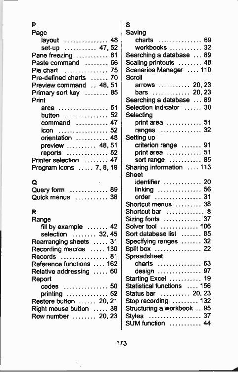
P

Pagelayout 48set-up 47, 52

Pane freezing 61

Paste command 56Pie chart 75Pre -defined charts 70Preview command 48, 51Primary sort key ..... 85Print

area 51

button 52command 47icon 52orientation 48preview 48, 51reports 52

Printer selectionProgram icons 7, 8, 19

QQuery form 89Quick menus 38

RRange

fill by example 42selection 32, 45

Rearranging sheets 31

Recording macros 130Records 81

Reference functions .... 162Relative addressing 60Report

codes 50printing 52

Restore button 20, 21Right mouse button 38Row number 20, 23

SSaving

charts 69workbooks 32

Searching a database 89Scaling printouts 48Scenarios Manager .... 110Scroll

arrows 20, 23bars 20, 23

Searching a database 89Selectioi indicator 30Selecting

print area 51

ranges 32Setting up

criterion range 91

print area 51

sort range 85Sharing informatior .... 113Sheet

identifier 20linking 56order 31

Shortcut menus 38Shortcut bar 8

Sizing fonts 37Solver tool 106Sort database list 85Specifying ranges 32Split box 22Spreadsheet

charts 63design 97

Starting Excel 19Statistical functions .... 156Status bar 20, 23Stop recording 132Structuring a workbook .. 95Styles 37SUM function 44

173

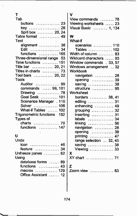
TTab

buttons 23key 26Split box 20, 24

Table format 49Text

alignment 36Edit 34functions 165

Three-dimensional range 53Time functions 151Title bar 20, 21Titles in charts 73Tool bars 20, 22Tools

Auditor 99commands 99, 101Drawing 78Goal Seek 101Scenarios Manager 110Solver 106What -if Tables 102

Trigonometric functions 152Types of

charts 70functions 147

U

Undoicon 46feature 34

Unfreeze panes 62Using

database forms 89functions 43macros 129Office Assistant 12

VView commands 78Viewing worksheets 23Visual Basic 1, 134

What -ifscenarios 110Tables 102

Width of column 83Wildcard characters 93Window commands . 33, 57Windows arrangement .. 32Workbook

navigation 28opening 39saving 38structure 95

Worksheetborders 38, 41editing 31

enhancing 49grouping 32inserting 31

labels 34linking 56navigation 28opening 39printing 47range selectionsaving

32, 4538

Viewing 33XXY chart

z

71

Zoom view 83

174

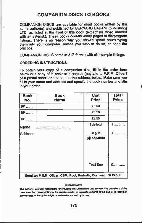
COMPANION DISCS TO BOOKS

COMPANION DISCS are available for most books written by thesame author(s) and published by BERNARD BABANI ,:publishing)LTD, as listed at the front of this book (except for those markedwith an asterisk). These books contain many pages of file/programlistings. There is no reason why you should spend hours typingthem into your computer, unless you wish to do so, or need thepractice.

COMPANION DISCS come in 3W' format with all example listings.

ORDERING INSTRUC-IONS

To obtain your copy of a companion disc, fill in the order formbelow or a copy of it, enclose a cheque (payable to P.R.M. Oliver)or a postal order, and send it to the address below. Make sure youfill in your name and acdress and specify the book number and titlein your order.

BookNo.

BookName

UnitPrice

TotalPrice

BP £3.50

BP £3.50

BP £3.50

Name

Address:

Sub -total

P & P

(@ 45p/disc)

Total Due

£

£

£

Send to: P.R.M. Oliver, CSM, Pool, Redruth, Cornwall, TR15 3SE

PLEASE NOTEauthor(s) are fully responsible fa providing this Companion Disc service. The publishe-s of this

book accept no responsibility for the supply, duality, or magnetic contents of the disc, or in respect ofany damage, or injury that might 1>:. suffered or caused by its use

175

Babani Computer Books

MS -Excel 97 explainedIf you are a PC user and want to learn how to usethe 3D Excel 97 spreadsheet, then this book willteach you how to do just that in the shortest andmost effective way. The book was written with boththe newcomer to spreadsheets and the existingspreadsheet user in mind.The book explains:-. How to build up simple spreadsheet examples, edit

entries, format cells and ranges, and save and openworksheets.

. How to generate and use 3 -dimensional work-sheets and how to link them together.

. How to generate and add graphs to a worksheet,edit, preview and print the result.

. How to set up and query a database managementsystem.

. How to record a simple macro, and how to under-stand and use Visual Basic code.

. How to use the Auditor, Goal Seek, What -if Tables,Solver and What -if Scenarios.

. How to share information with other applications bylinking, embedding and using hyperlinks

Beginners Q Intermediate IN Advanced

BP 429

i6.99

11111111M11111111

9

ISBN 0-85934-429-0

78 085 911 1

344296

0i0 6 9 9>