monetary policy and stock market movements in turkey
TRANSCRIPT
School of Economics and Finance
Queen Mary University of London
MONETARY POLICY AND STOCK MARKET MOVEMENTS IN TURKEY
Izzet Onur SERAKIBI
Email Address
M.Sc. in Business Finance
August,2013
I.TABLE OF CONTENTS:I.TABLE OF CONTENTS:.............................................2
II.ABSTRACT:.....................................................4
1-INTRODUCTION:..................................................4
2.A BRIEF REVIEW OF THE LITERATURE ON THE MONETARY POLICY AND ASSET PRİCE RELATIONS:...........................................6
2.1.The Taylor Rule:.............................................7
2.1.1. Specification of the Taylor Rule:.........................9
2.1.1.1. Estimation Data:........................................9
2.1.1.2. A Brief Information About Turkish Stock Market:.........9
2.1.1.2.1. The Credit Outlook of Turkey as an Investment Criteria:................................................................10
2.1.1.3.The Standart Taylor Rule:...............................10
2.1.1.4.The Augmented Taylor Rule:..............................11
2.1.1.5. Forward Looking Models and Generalized Method of Moments:................................................................11
2.1.2. Estimation of the Taylor Rule:..........................12
2.1.2.1. Graphical Inspection of the Data:......................12
2.1.2.2. Standart Taylor Rule with Ordinary Least-Squares Method:...............................................................14
2.1.2.3. The Wald Test:.........................................15
2
2.1.2.4.Visual Impression Regarding the Model:..................16
2.1.2.5.Chow Breakpoint Test:...................................16
2.1.2.6. Estimating The Augmented Taylor Rule:..................17
2.1.2.6.1.Ordinary Least-Squares Analysis (ATR):................17
2.1.2.6.2. Diagnostic- Normality Test:..........................18
2.1.2.6.3. Diagnostic- Heteroskedasticity Test:.................19
2.1.2.6.4. Diagnostic- Breusch-Godfrey Serial Correlation LM Test:................................................................19
2.1.2.6.5. Ordinary Least Squares Method (Newey-West Option):. . .19
2.1.2.6.6. Generalized Method of Moments(GMM) Estimator:........21
3.CONCLUSION:...................................................22
REFERENCES......................................................24
3
II.ABSTRACT:
In this dissertation, we investigate the hypothesis that
monetary policy responds to movements in asset prices.In the study
the arguments in favor and against the above hypothesis will be
studied, the empirical framework will be discussed and the
hypothesis will be tested. In the investigation, we adopt the
Taylor rule as the empirical framework and used its standard and
augmented versions in order to reach a conclusion.In this study,
we will especially explore that whether the stock market movements
play a crucial role in shaping monetary policy either directly or
indirectly in Turkey between the years 1997 and 2012.
4
1-INTRODUCTION:
Turkish economy showed an outstanding performance between the
years of 1997 and 2012.During the period, the inflation rate
dropped to %6.16 from %85 and parallel to the inflation rate
interest rate dropped almost %60 while GDP rose almost %4 annually
in average. Additionally BIST100, the stock market value of Turkey
rose almost 60% in 2012 and reached the 80.000 index level while
it was only at 1.613 index level at 1997.
The objective of this investigation is to test the hypothesis
that monetary policy responds to movements in asset prices. In
this study, we will try to prove that there is a significant
correlation between monetary policy and asset pricing.Policy rules
of central bank of Turkey and reflections of those decisions in
the stock market between the period of 1997 and 2012 will be the
main investigation subject of this study.
According to Bernanke and Mihov (1998) the process by which
the central banks control the money supply in order to keep the
interest rate at certain levels for promoting economic growth and
price stability is called monetary policy.The need to the central
banks in providing a stable economic outlook has increased during
the last years. So as a policy maker, central banks should
struggle with inflation as well as they should prevent the markets
from the financial crisis.
5
Bernanke (2000) also claims that inflation is no longer a
great issue to concern about since the world’s leading central
banks have been very successful at keeping it under control over
the past twenty years. Nowadays an apparent increase in financial
instability and increased volatility of asset prices seem to be
the next battles facing central banks.
According to Mishkin (2012) mismanagement of financial
liberalization and asset-price booms and busts can trigger
financial crises which usually results in failures of major
financial institutions and increased uncertainty in the financial
markets.When investor psychology affects the assets prices such
as equity shares and real estate above their fundamental economic
values, the rise of asset prices called as an asset-price bubble.
Those bubbles in asset prices are often driven by credit booms
which are usually supported by the policies of the central banks.
Allen and Gale (2000) argue that the recent financial crises
which was caused by the bubble of asset prices is resulted with
widespread defaults of some leading financial institutions. The
money borrowed from banks for asset investment is always
attractive for investors who plan to default on the loan rather
than making safe but small amounts of profit in their investments.
At the times of financial fragility, the risk appetite of the
investors in both the real and financial sectors investments can
lead the asset prices to very high levels and cause crisis due to
the insufficient positive credit expansion.
6
There have been two major asset bubble crisis in 1929 and 1980
at the last century.Both of them caused protracted recessions and
deflation.According to Bordo and Jeanne (2002) The policy makers
have a perennial interest in the relation of monetary policy and
asset price movements since it is essential to decide whether
trying to prevent the results of an asset market collapse before
it turns to a financial crisis or whether it was more effective to
react the asset prices after financial markets completely went
down.
Bean (2004) claims that in the aftermath of the recent crisis
caused by asset price bubbles in Japan and U.S. the most popular
debate between central bankers and academic circles was the role
of the asset prices in the setting of monetary policy. Views of
Gilchrist and Leahy (2002) remind the following period of
increased volatility in asset prices in Japan and US.Then most of
the economists had called for central banks to respond to asset
price volatility against to large swings in growth rates.
2.A BRIEF REVIEW OF THE LITERATURE ON THE MONETARY POLICY AND ASSET PRİCE RELATIONS:
The role of asset price movements in shaping monetary policy
can be explained by two opposite view in the literature. Some
economist such as Bernanke and Gertler (2001) and Vickers (1999)
claim that there is no need to believe in asset price volatility
as a key determinant for setting monetary policy but on the other
hand, Cecchetti, Genberg and Wadhwani (2002) believe volatility in
7
asset prices can help central banks when shaping monetary policy
by providing more information.
According to Bernanke and Gertler (2001) the appropriate
position of asset prices in the monetary policy has been witnessed
to many debates. The question of whether central banks should
respond to volatility in asset prices or not can be answered by
the inflation-targeting approach. According to this view
volatility in asset prices may affect the monetary policy if only
the expected inflation rate is affected negatively from those
movements. For instance, a bubble in asset prices can increas the
aggregate demand by increasing consumers wealth and affect the
inflation negatively.Furthermore, once the effects of asset prices
in the general price level have been accounted for central banks
should not response the changes in the asset prices anymore. This
is a crucial point in monetary policy because this kind of
attempts to influence asset prices can affect the investors
psychology and lead the markets unpredictable future.
According to Cecchetti et al. (2002), it is possible to
improve macroeconomic performance by reacting to asset price
misalignments systematically. Just by setting policy rates with an
eye toward particularly in misalignments and generally in asset
prices can help to smooth output and inflation fluctuations.
Distortions in investment and consumption created by asset price
bubbles can cause excessive increases followed by severe falls
in both inflation and GDP. To raise interest rates when asset
prices rise above the expected levels and to lower them modestly
8
when asset prices fall below the reasonable levels will help
central banks to offset the impact on inflation and output gap of
these bubbles. The important outcome of this kind of monetary
policy is to show the markets that central banks can take the
necessary measurement in this way. The probability of bubbles in
equity prices might be reduced and a contribution to greater
macroeconomic stability would also be provided by this method.
Bernanke and Gertler (2001), claim whether the volatility in
asset prices is the result of bubbles or technological shocks, an
aggressive inflation-targeting policy stabilizes output and
inflation. In their opinion the study of Cecchetti et al. ignores
the fact of shocks other than bubble shocks and the probabilistic
nature of the bubble. Their theory lies on the assumption of a
bubble shock which lasts precisely five periods. Also, the
knowledge of the central banks about the reasons and the bursting
moment of the bubbles are both highly unlikely conditions. A
panic-driven financial instability that could affect the economy
negatively can be reduced and macroeconomic stability can be
sustained by inflation targeting monetary policy. In the end, they
conclude for plausible parameter values the central banks should
not respond to asset prices.
On the other hand, Cecchetti et al.(2002) claims that the
underlying sources of shocks to the economy determines the
relationship between fluctuations in asset prices on the one hand,
and output and inflation on the other. So they suggest that
monetary authority should not interfere to all changes in asset
9
prices mechanically and in the same way. Since the private sector
might possess more information about equilibrium valuations of
asset prices, it would be possible to react anything from asset
price fluctuations that can help to shape monetary policy.
Cecchetti et al. (2002) also claims that not all asset price
changes, but the asset price instability should be identified and
responded in an inflation-targeting strategy. That means stock
market value should be included in the information sets in order
to be processed by the central bank just as well as the output
gap. The problem of to differentiate the asset price movements
and to realize whether they are justified by underlying
fundamentals or not is the main challenge of the policymakers.
2.1.The Taylor Rule:
As a major tool of monetary policy central banks should
change the interest rate in order to provide macro economic
stability first and then keep the employment in maximum
levels.Taylor rule which was proposed by world renowned monetary
economist John B. Taylor and named after him can help central
banks with the question of how much would it be the optimum
interest rate. Taylor principle is a different aspect of taylor
rule and stipulates that the nominal interest rate should be raise
more than the increase in the inflation rate.
According to Castro (2008) to set up the interest rate past
or current values of inflation and output gap is a commonly used
method by central banks.In its very original form, the main
10
objectives of the Taylor rule are providing the price stability
and keeping the economy moving towards maximum employment.In order
to keep the general price level stable Taylor rule simply
recommends that when the inflation rate is exceeded the target
level central banks should rise the interest rate above the level
of the stabilizing rate and when it is below the target level
interest rate should be decreased to the levels below the
target.In order to accomplish the second objective of the Taylor
rule it is suggested that the interest rate should be determined
above the stabilizing rate when real GDP is above the target. If
real GDP is below the potential real GDP Taylor, recommends that
the interest rate should be reduced below the stabilizing rate.
According to Taylor (1993) conducive monetary policy requires
to put equal weights on the impact of inflation and GDP since
putting more weight on the inflation gap could be a sign of more
aggressive policy to target inflation by the central banks.
Godhart and Hofmann (2000) believe that the question of how
asset price volatility should be considered in principle for
objectives of monetary policy is subject to a consensus among
leading economists.An inflation target which can also be defined
as achieving price stability is the primary objective of the
central banks while inflation is a price index which consist of
current goods and services but excludes assets prices directly.
11
Frait and Komarek (2006) point out that asset price
developments are usually taken into account when refining monetary
policy, even if central banks formally targets price stability.
The reason for this approach lies on the fact that asset price
movements, especially physical assets, can impact on CPI inflation
by tempting the people to invest in those assets.Once people
starts buying those assets the production of the assets rises as
well as the demand for the raw materials and this cycle triggers
the CPI inflation.
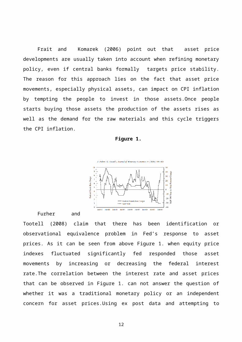
Figure 1.
Furher and
Tootell (2008) claim that there has been identification or
observational equivalence problem in Fed’s response to asset
prices. As it can be seen from above Figure 1. when equity price
indexes fluctuated significantly fed responded those asset
movements by increasing or decreasing the federal interest
rate.The correlation between the interest rate and asset prices
that can be observed in Figure 1. can not answer the question of
whether it was a traditional monetary policy or an independent
concern for asset prices.Using ex post data and attempting to
12
identify the effects of asset prices on monetary policy may have a
misleading impact.
2.1.1. Specification of the Taylor Rule:
Many scholars all around the world highly interested and used
the Taylor rule in the past years.Since it can provide an answer
to how to set monetary policy by a simple method in this study,
“the Taylor rule” will be the econometric framework that is going
to be used in the analysis.
2.1.1.1. Estimation Data:
As we mentioned above in this study, the Taylor rule will be
used as the estimation framework as well as some of the Turkish
economic data ranging from 1997:1Q to 2012:4Q., will be used as
the estimation data.In the study we will apply RGDP, which is the
Turkish real GDP, CPI, which is the consumer price index of Turkey
, interest is the interest rate, set by the Central Bank of Turkey
and BIST100 which is the stock market value of Turkey to our
model to estimate the Taylor rule.
The data which we need to carry out our study including GDP,
CPI, Interest Rates and BIST100 index of Turkey were extracted
from International Monetary Fund International Financial
Statistics via UK Data Service international macrodata.
2.1.1.2. A Brief Information About Turkish Stock Market:
First time in Turkish history on January 3, 1986 stock trading
started at the Cağaloğlu building of Istanbul Stock Exchange
13
(IMKB) with a number of 80 listed companies.On October,1992 IMKB
was accepted to The World Federation of Exchanges as a full
member. The legal framework of Turkish capital markets, consist of
Capital Markets Law (CML) and Turkish Commercial Code.The more
detailed regulations are manifested as Communiqués of Capital
Markets Board and Regulations of Stock Exchange. In order to
harmonize the Turkish capital markets regulation with the EU
acquis, the Capital Markets Law No. 6362 was enacted by the
Turkish law maker.With that amendment in Capital Markets Law
Turkish government also aimed to liberalize the activity of
running organized markets and re-brand IMKB as Borsa Istanbul
(BIST).After the recent changes in the Capital Markets Law Borsa
Istanbul is now subject to private law as a joint-stock company.
Borsa Istanbul (2013).
By the end of 2012, the number of the traded companies on BIST
reached to 404 while it was 258 at 1997. Under the name of Borsa
Istanbul, two major national indices are existed. SERPAM (2013).
Those are BIST30 and BIST100.BIST30 is consisted of 30 large
companies by the value of outstanding shares traded in the stock
market. Financial institutions and a couple of leading holding
companies are examples of firm types of the BIST30.BIST100 is the
major index of Borsa Istanbul.It is consisted of BIST30 and the
following largest industrial companies by the value of outstanding
shares traded in the stock market. Usually BIST30 companies have
higher beta value than BIST100 companies and BIST30 index also
considered as a more reliable indicator about the general trend of
the markets.
14
2.1.1.2.1. The Credit Outlook of Turkey as an Investment Criteria:
By the august of 2013, the long-term foreign-currency credit
rating of Turkey was confirmed as BB+ by S&P, BBB- by Fitch and
Baa3 by Moody’s. Moody’s and Fitch already upgraded Turkey’s
foreign-currency sovereign credit rating to the investment
grade.Another foreign-currency sovereign credit rating upgrade is
expected by S&P which will lift the general credit outlook of
Turkey to the investment grade in foreign-currency.
2.1.1.3.The Standart Taylor Rule:
The Taylor rule which formulates the linear relation between
inflation ,GDP and the interest rate was established by John B.
Taylor in 1993.At this point of the study, the very first step of
our econometric analysis consists of estimating the standard
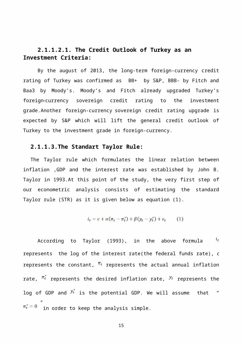
Taylor rule (STR) as it is given below as equation (1).
According to Taylor (1993), in the above formula
represents the log of the interest rate(the federal funds rate), c
represents the constant, represents the actual annual inflation
rate, represents the desired inflation rate, represents the
log of GDP and is the potential GDP. We will assume that “
” in order to keep the analysis simple.
15
2.1.1.4.The Augmented Taylor Rule:
Among the monetary policy makers two opposite views emerged
regarding how to set a well refined monetary policy. According to
the first view monetary authority should not respond to movements
in asset prices and wait for to see the progress in the economic
data such as the inflation rate. On the other hand, stock market
movements could help to predict the future fluctuations in the
monetary markets and the augmented Taylor rule which is employed
by monetary authorities would be the best econometric framework
for this purpose.
The second step of the econometric analysis will be estimating
the augmented Taylor rule. In the 1main literature, asset price
volatility suppose to bring more information to the central banks
and by doing so it could affect the decisions of the monetary
authority.According to Castro (2008) a financial conditions index
containing data from stock market movements can be included in the
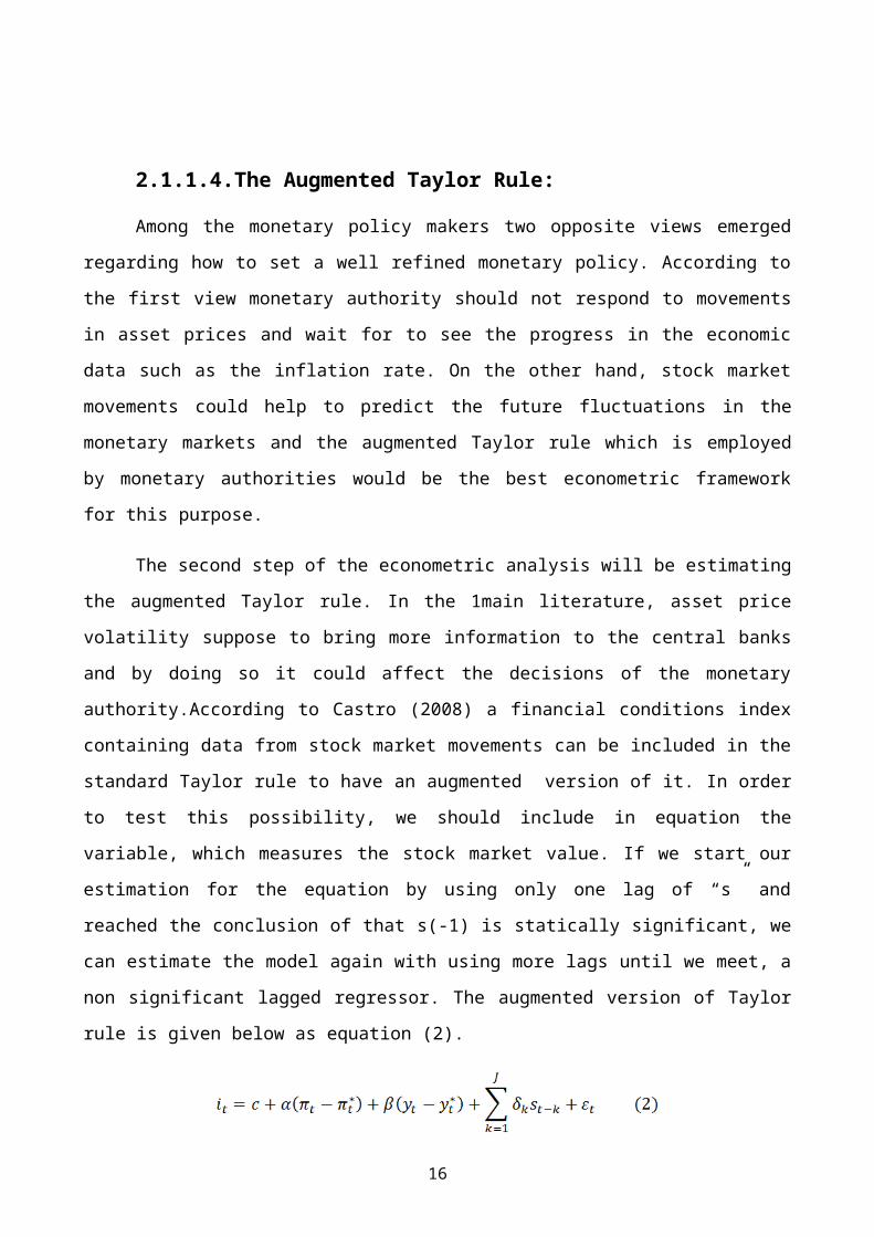
standard Taylor rule to have an augmented version of it. In order
to test this possibility, we should include in equation the
variable, which measures the stock market value. If we start our
estimation for the equation by using only one lag of “s” and
reached the conclusion of that s(-1) is statically significant, we
can estimate the model again with using more lags until we meet, a
non significant lagged regressor. The augmented version of Taylor
rule is given below as equation (2).
16
2.1.1.5. Forward Looking Models and Generalized Method of Moments:
As John Maynard Keynes (1923) once said that we might have
been too late if we would have waited until a price movement was
actually very close before taking some measurements. This words
reflect the importance of the forward-looking models in monetary
policy. When private economic actors change their economic
behavior in a particular economic subject some variables such as
long-term interest rates may be changed. According to Kamada and
Muto (2000) this mechanism of expectation formation is generally
called as rational expectations models while the models that
integrated with such expectations regardless current and past
information are called as forward looking models. Mavroeidis
(2004) points out that since they based on micro-foundations and
built on rational expectations, generalized method of moments
(GMM) methods have become popular for estimating forward-looking
models.
The third step of the econometric analysis will be estimating
our model by GMM. This is a general estimation method which is
derived from the method of moment. It is developed by Lars Peter
Hansen in 1982. Many other estimators can be considered as special
cases of generalized method of moments. It can allow economic
models to be specified without making unwanted assumptions. It is
consistent and asymptotically normal. In order to produce
estimates of the unknown parameters of the model it combines
17
observed data with the information extracted from orthogonality
conditions. Hansen (2007) also points out that it can be used when
maximum likelihood estimation is not applicable and the parameter
of interest is finite-dimensional. Its properties of taking
account of both sampling and estimation error and being
constructed without specifying the full data generating process
made generalized method of moments a widely used estimator.
2.1.2. Estimation of the Taylor Rule:
The main purpose of this exercise is to test whether the
stock market movements play a crucial role in shaping monetary
policy either directly or indirectly.
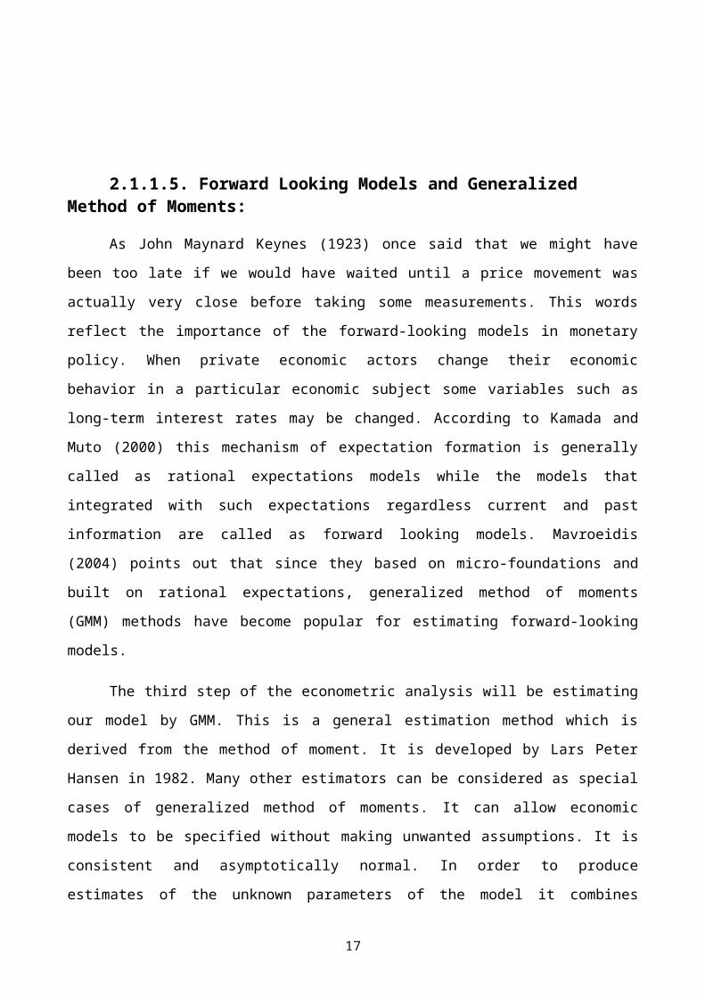
2.1.2.1. Graphical Inspection of the Data:
The below figure depicts the movements in interest rate
between the years of 1997 and 2012.During this period interest
rate decreased significantly.It remained stable with slight
changes between 2005 and 2009 and continued to incline afterward.
From the second half of the 1997 to 2012 it dropped almost 60%.
Figure 2.
10
20
30
40
50
60
70
97 98 99 00 01 02 03 04 05 06 07 08 09 10 11 12
IR
18
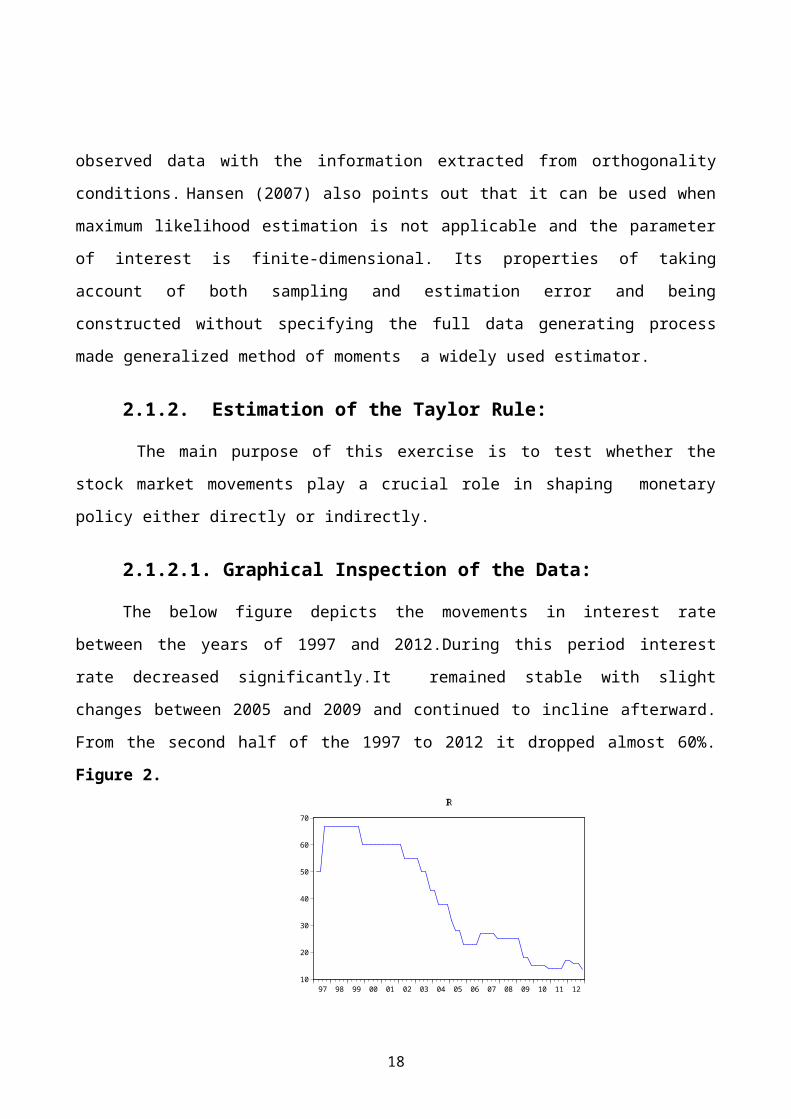
The below figure depicts the movements in GDP quarterly
between the years of 1997 and 2012.During this period, GDP of
Turkey increased significantly and reached almost 1.500 Billion
Turkish Lira annually by 2012.During the period, it negatively
correlated with the interest rate.
Figure 3.
0
50,000
100,000
150,000
200,000
250,000
300,000
350,000
400,000
97 98 99 00 01 02 03 04 05 06 07 08 09 10 11 12
GDP
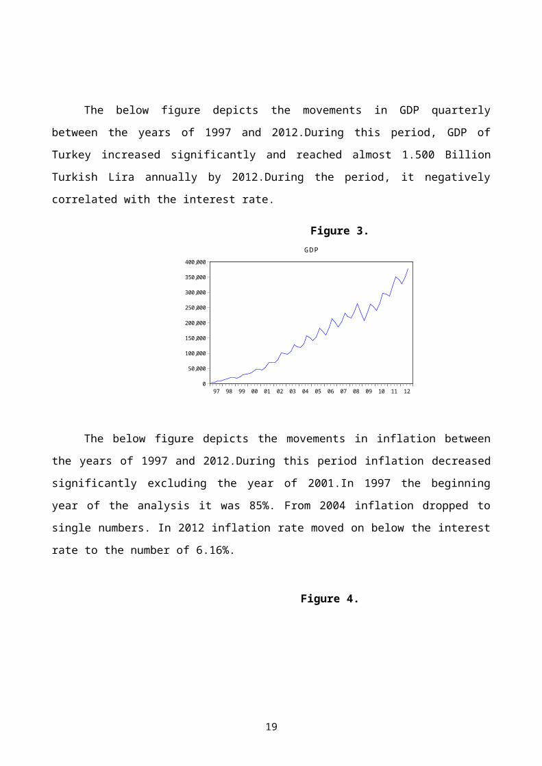
The below figure depicts the movements in inflation between
the years of 1997 and 2012.During this period inflation decreased
significantly excluding the year of 2001.In 1997 the beginning
year of the analysis it was 85%. From 2004 inflation dropped to
single numbers. In 2012 inflation rate moved on below the interest
rate to the number of 6.16%.
Figure 4.
19
0
10
20
30
40
50
60
70
97 98 99 00 01 02 03 04 05 06 07 08 09 10 11 12
INFLATIO N
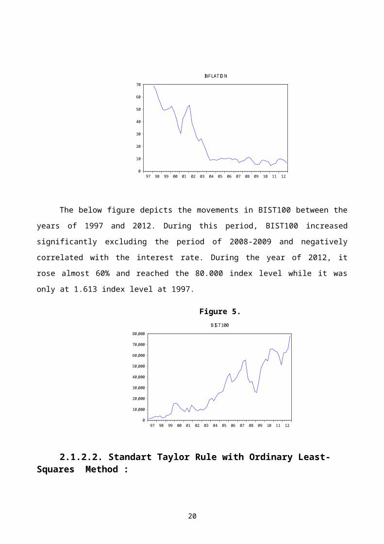
The below figure depicts the movements in BIST100 between the
years of 1997 and 2012. During this period, BIST100 increased
significantly excluding the period of 2008-2009 and negatively
correlated with the interest rate. During the year of 2012, it
rose almost 60% and reached the 80.000 index level while it was
only at 1.613 index level at 1997.
Figure 5.
0
10,000
20,000
30,000
40,000
50,000
60,000
70,000
80,000
97 98 99 00 01 02 03 04 05 06 07 08 09 10 11 12
BIST100
2.1.2.2. Standart Taylor Rule with Ordinary Least-Squares Method :
20
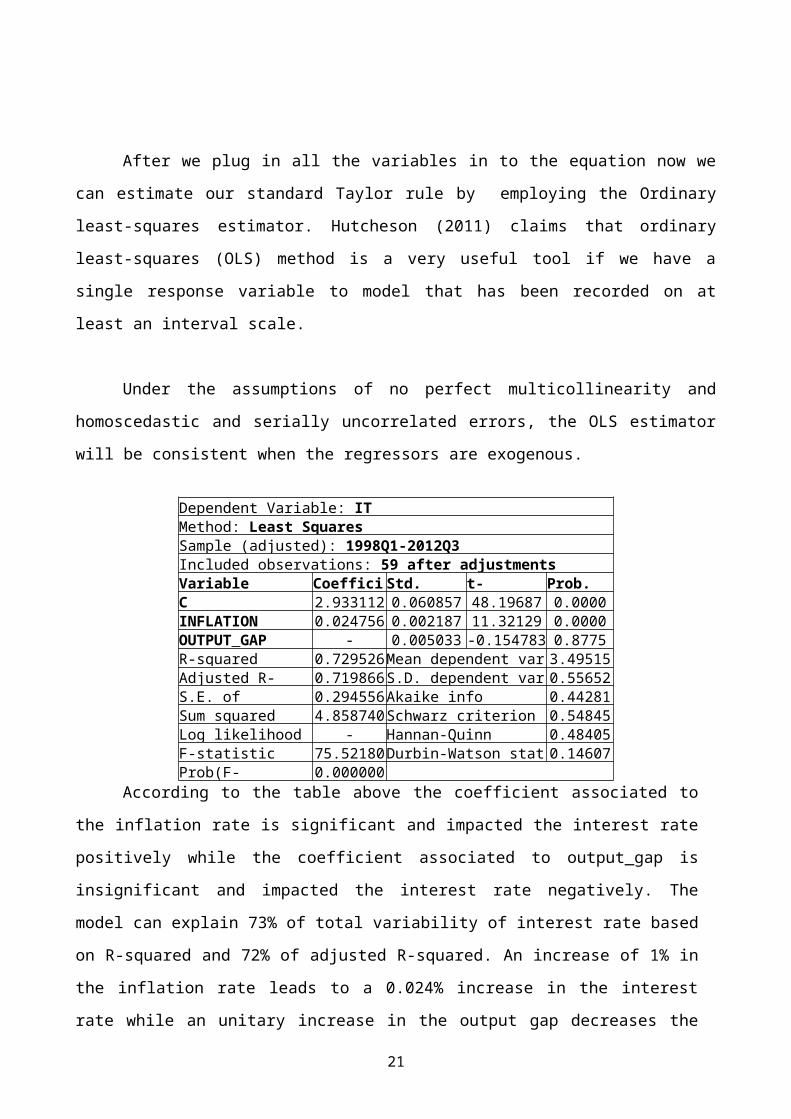
After we plug in all the variables in to the equation now we
can estimate our standard Taylor rule by employing the Ordinary
least-squares estimator. Hutcheson (2011) claims that ordinary
least-squares (OLS) method is a very useful tool if we have a
single response variable to model that has been recorded on at
least an interval scale.
Under the assumptions of no perfect multicollinearity and
homoscedastic and serially uncorrelated errors, the OLS estimator
will be consistent when the regressors are exogenous.
Dependent Variable: ITMethod: Least SquaresSample (adjusted): 1998Q1-2012Q3Included observations: 59 after adjustmentsVariable Coeffici Std. t- Prob.C 2.933112 0.060857 48.19687 0.0000INFLATION 0.024756 0.002187 11.32129 0.0000OUTPUT_GAP - 0.005033 -0.154783 0.8775R-squared 0.729526Mean dependent var 3.49515Adjusted R- 0.719866S.D. dependent var 0.55652S.E. of 0.294556Akaike info 0.44281Sum squared 4.858740Schwarz criterion 0.54845Log likelihood - Hannan-Quinn 0.48405F-statistic 75.52180Durbin-Watson stat 0.14607Prob(F- 0.000000
According to the table above the coefficient associated to
the inflation rate is significant and impacted the interest rate
positively while the coefficient associated to output_gap is
insignificant and impacted the interest rate negatively. The
model can explain 73% of total variability of interest rate based
on R-squared and 72% of adjusted R-squared. An increase of 1% in
the inflation rate leads to a 0.024% increase in the interest
rate while an unitary increase in the output gap decreases the
21
interest rate by -0.000779%. In the model, the constant is
positive and indicates that when the output_gap and inflation are
zero, the stabilizing interest rate would be at the rate of
2.933112.The probability of F-statistic is zero which is a value
that support the correctness of the model and shows that our
regressors are jointly different from zero.According to this
argument the null hypothesis can be rejected.The final conclusion
of the OLS test points out that there might be a serial
correlation problem in the model since the DW statistic is more
than 10%.
2.1.2.3. The Wald Test:
Engle (1984) points out that in order to test the
aforementioned restriction, we need to set a Wald test which is
based upon Wald’s elegant analysis upon asymptotic approximation
to the T and F tests in econometrics.
According to Taylor (1993) output gap and the inflation own an
equal weight in shaping monetary policy.In order to do that both
second and third coefficient should be set equal to 50% The
Central Banks that adopts a more severe inflation targeting
policy should put more weight on inflation compared to the output
gap.According to that argument when we set the restriction as
all the coefficients are equal to 50%.The variations in the
dependent variable can not be explained by the independent
variables.
22
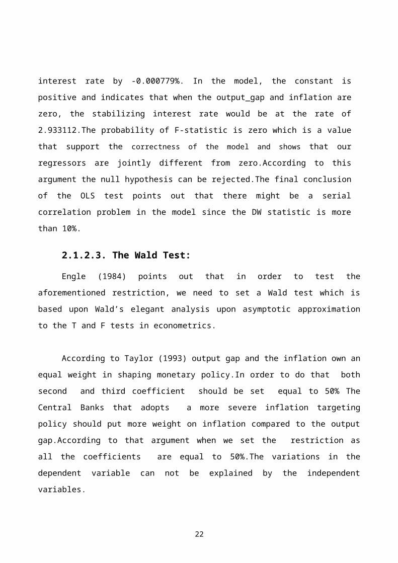
Wald Test:Equation: UntitledTest Value df ProbabilF-statistic 44354.99 (2, 56) 0.0000Chi-square 88709.98 2 0.0000
According to the table above the p-values associated to the F-
test and Chi-square are equal to 0.00. Since it is less than 10%
we can reject the null hypothesis that claims output gap and the
inflation own an equal weight in shaping monetary
policy.Therefore, we may conclude that all the regressors are
jointly significant and inflation and output gap weight
differently in shaping monetary policy.
2.1.2.4.Visual Impression Regarding the Model:
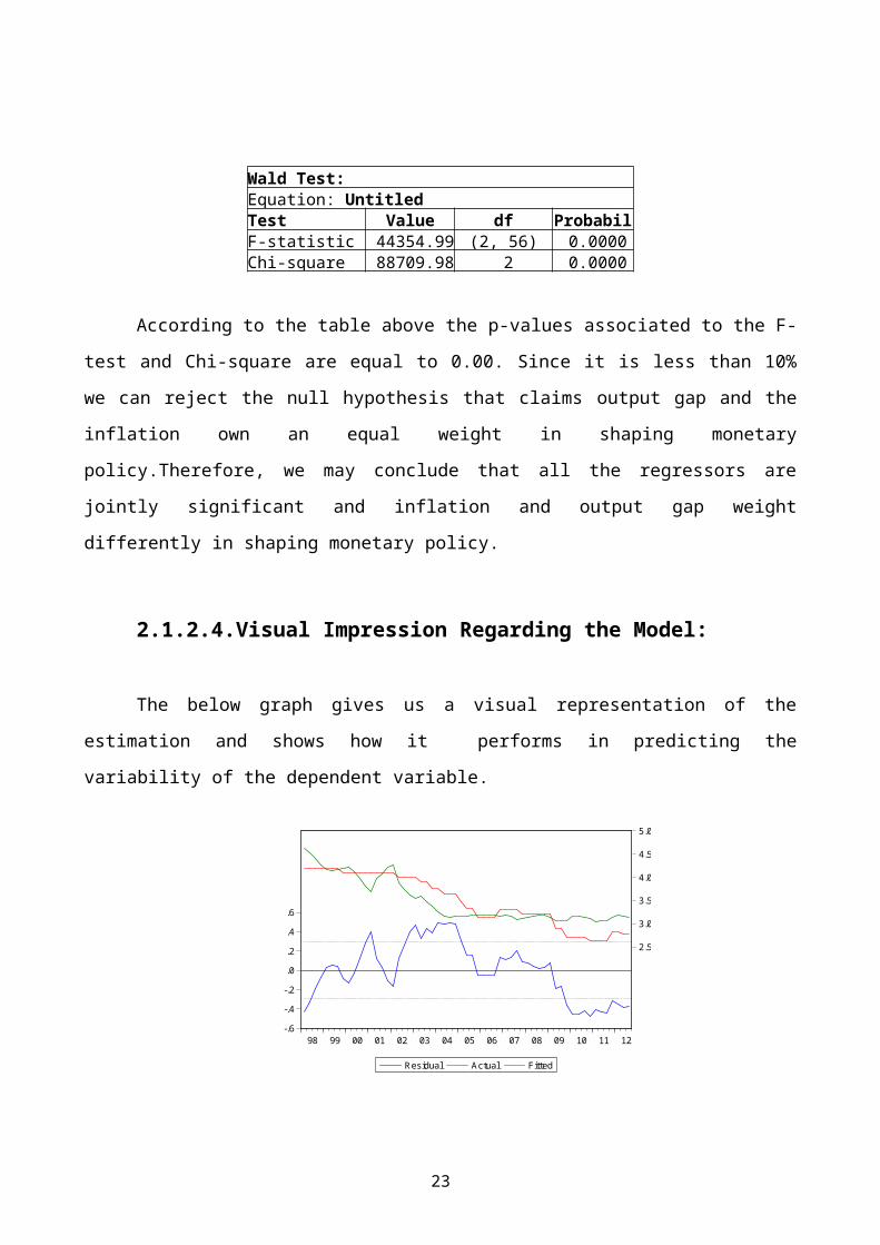
The below graph gives us a visual representation of the
estimation and shows how it performs in predicting the
variability of the dependent variable.
-.6
-.4
-.2
.0
.2
.4
.6
2.5
3.0
3.5
4.0
4.5
5.0
98 99 00 01 02 03 04 05 06 07 08 09 10 11 12
Residual Actual Fitted
23
The above model consistently underestimates the actual
interest rate from 1998 to 2009 while it overestimates it from
2009 onwards. Since the residual do not seem to be i.i.d. , we can
conclude the regression model misses something.
2.1.2.5.Chow Breakpoint Test:
On the basis of the visual representation of the estimation, a
possibility of omitted variables problem may rise. At this point
of the study, the presence of some shocks that can affect the
stability of the relationship under investigation will be checked
by chow breakpoint test.
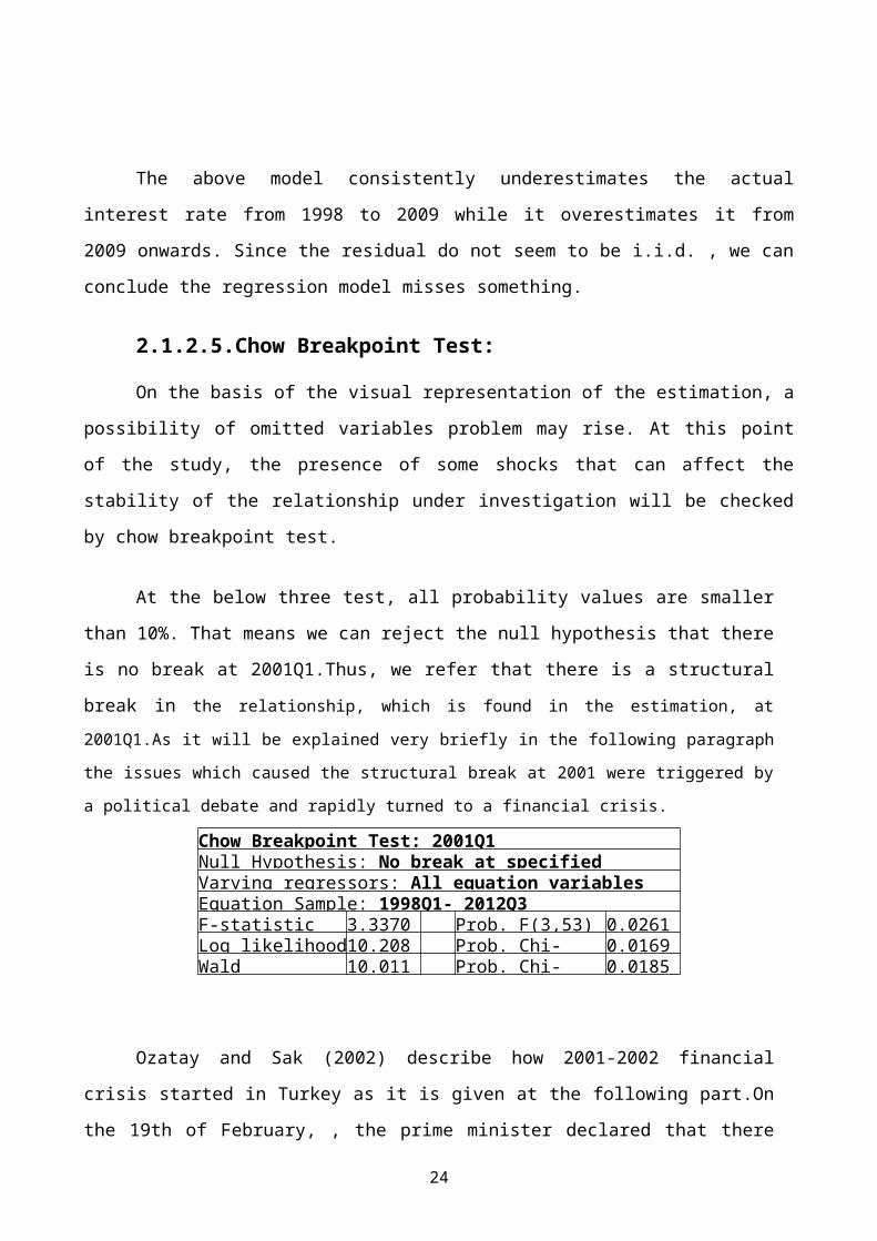
At the below three test, all probability values are smaller
than 10%. That means we can reject the null hypothesis that there
is no break at 2001Q1.Thus, we refer that there is a structural
break in the relationship, which is found in the estimation, at
2001Q1.As it will be explained very briefly in the following paragraph
the issues which caused the structural break at 2001 were triggered by
a political debate and rapidly turned to a financial crisis.
Chow Breakpoint Test: 2001Q1 Null Hypothesis: No break at specified Varying regressors: All equation variablesEquation Sample: 1998Q1- 2012Q3F-statistic 3.3370 Prob. F(3,53) 0.0261Log likelihood10.208 Prob. Chi- 0.0169Wald 10.011 Prob. Chi- 0.0185
Ozatay and Sak (2002) describe how 2001-2002 financial
crisis started in Turkey as it is given at the following part.On
the 19th of February, , the prime minister declared that there
24
was political conflict between him and the President soon after
he left the National Security Council meeting.After this
announcement the over-night rate increased to 2058% on the
following day and 4019% on the 21th of February.The banking
sector rushed to foreign currency. Since the US markets were closed
at that specific date, the Central Bank could not satisfy the foreign
currency demand of the banking sector.After the announcement about the
country was switching to a freely floating exchange rate system the
dollar rate jumped almost 40%.
2.1.2.6. Estimating The Augmented Taylor Rule:
As we mentioned before on chapter 2.1.1.4. according to
Castro (2008) a financial conditions index containing data from
the stock market movements can be included in the standard Taylor
rule to have an augmented version of it by including in equation
the variable “s” which measures the stock market value.The
augmented version of Taylor rule (ATR) is given below as equation
(2).
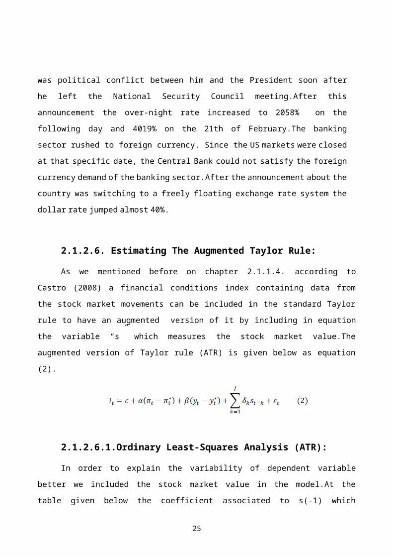
2.1.2.6.1.Ordinary Least-Squares Analysis (ATR):
In order to explain the variability of dependent variable
better we included the stock market value in the model.At the
table given below the coefficient associated to s(-1) which
25
represents the stock market value is negative and insignificant.It
can also be observed from the table that the goodness of fit of
the model increased very slightly after we include the first lag
of “s”.When we look at the R-squared, we can see it increased from
0.729 to 0.735 while adjusted R-squared increased from 0.719 to
0.720, which shows that our model can explain a little bit better
the variability of the dependent variable.Including the stock
market value did not contribute to the model to explain the
relations between interest rate and stock market value.
Dependent Variable: ITMethod: Least SquaresSample (adjusted): 1998Q2 -2012Q3Included observations: 58 after
Variable Coeffici Std. t- Prob. C 2.924457 0.062285 46.95252 0.0000
INFLATION 0.025980 0.002293 11.32999 0.0000OUTPUT_GAP - 0.005046 -0.078574 0.9377
S(-1) - 0.000849 -0.595461 0.5540R-squared 0.735205 Mean dependent 3.48292Adjusted R- 0.720494 S.D. dependent 0.55332S.E. of 0.292534 Akaike info 0.44600Sum squared 4.621117 Schwarz 0.58810Log likelihood - Hannan-Quinn 0.50135F-statistic 49.97701 Durbin-Watson 0.14855Prob(F- 0.000000
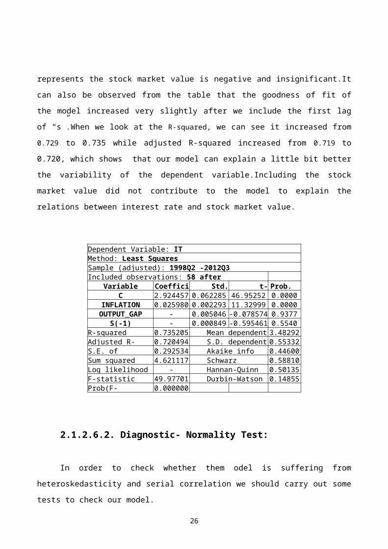
2.1.2.6.2. Diagnostic- Normality Test:
In order to check whether them odel is suffering from
heteroskedasticity and serial correlation we should carry out some
tests to check our model.
26
0
1
2
3
4
5
6
-0.4 -0.2 0.0 0.2 0.4
Series: ResidualsSample 1998Q3 2012Q3Observations 57
Mean 3.17e-16Median 0.003373Maximum 0.529819Minimum -0.462369Std. Dev. 0.279457Skewness 0.113068Kurtosis 2.172355
Jarque-Bera 1.748319Probability 0.417213
According to the above table of Jarque Bera test hypothesis of
normality in the distribution of the residuals can not be rejected
since the Jarque Bera probability value is insignificant.
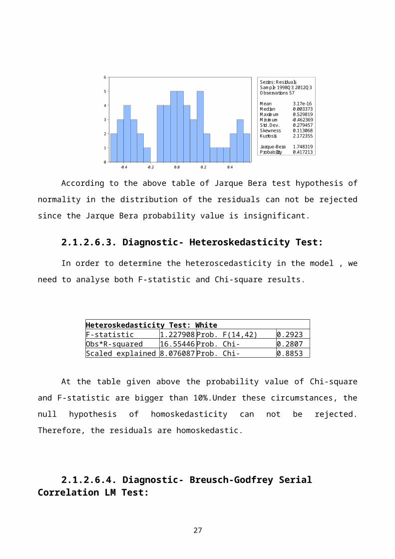
2.1.2.6.3. Diagnostic- Heteroskedasticity Test:
In order to determine the heteroscedasticity in the model , we
need to analyse both F-statistic and Chi-square results.
Heteroskedasticity Test: WhiteF-statistic 1.227908 Prob. F(14,42) 0.2923Obs*R-squared 16.55446 Prob. Chi- 0.2807Scaled explained 8.076087 Prob. Chi- 0.8853
At the table given above the probability value of Chi-square
and F-statistic are bigger than 10%.Under these circumstances, the
null hypothesis of homoskedasticity can not be rejected.
Therefore, the residuals are homoskedastic.
2.1.2.6.4. Diagnostic- Breusch-Godfrey Serial Correlation LM Test:
27
On the other hand, the below table shows that probability
value of both test statistic is 0.000. So now we can reject the
null hypothesis clearly and reach the conclusion of our model issuffering from serial correlation problem.
Breusch-Godfrey Serial Correlation LM Test:F-statistic 253.3161 Prob. F(1,51) 0.0000Obs*R-squared 47.44743 Prob. Chi- 0.0000
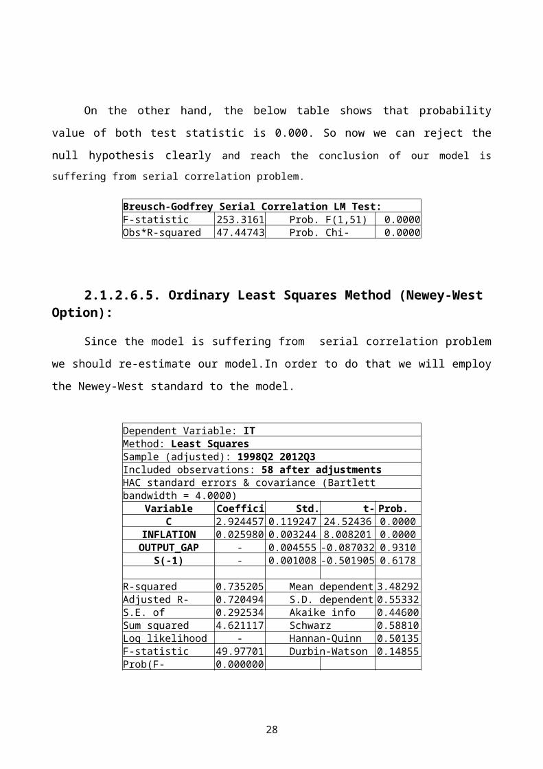
2.1.2.6.5. Ordinary Least Squares Method (Newey-West Option):
Since the model is suffering from serial correlation problem
we should re-estimate our model.In order to do that we will employ
the Newey-West standard to the model.
Dependent Variable: ITMethod: Least SquaresSample (adjusted): 1998Q2 2012Q3Included observations: 58 after adjustmentsHAC standard errors & covariance (Bartlett bandwidth = 4.0000)
Variable Coeffici Std. t- Prob. C 2.924457 0.119247 24.52436 0.0000
INFLATION 0.025980 0.003244 8.008201 0.0000OUTPUT_GAP - 0.004555 -0.087032 0.9310
S(-1) - 0.001008 -0.501905 0.6178
R-squared 0.735205 Mean dependent 3.48292Adjusted R- 0.720494 S.D. dependent 0.55332S.E. of 0.292534 Akaike info 0.44600Sum squared 4.621117 Schwarz 0.58810Log likelihood - Hannan-Quinn 0.50135F-statistic 49.97701 Durbin-Watson 0.14855Prob(F- 0.000000
28
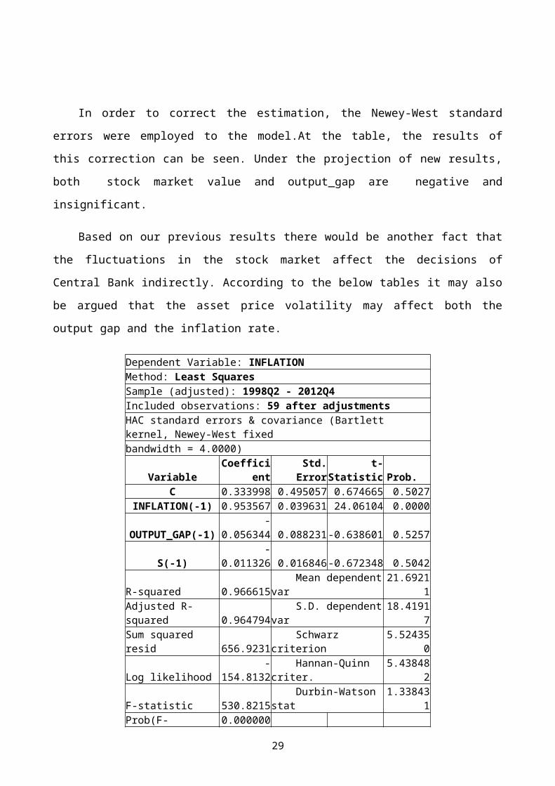
In order to correct the estimation, the Newey-West standard
errors were employed to the model.At the table, the results of
this correction can be seen. Under the projection of new results,
both stock market value and output_gap are negative and
insignificant.
Based on our previous results there would be another fact that
the fluctuations in the stock market affect the decisions of
Central Bank indirectly. According to the below tables it may also
be argued that the asset price volatility may affect both the
output gap and the inflation rate.
Dependent Variable: INFLATIONMethod: Least SquaresSample (adjusted): 1998Q2 - 2012Q4Included observations: 59 after adjustmentsHAC standard errors & covariance (Bartlett kernel, Newey-West fixedbandwidth = 4.0000)
VariableCoeffici
entStd.
Errort-
Statistic Prob. C 0.333998 0.495057 0.674665 0.5027
INFLATION(-1) 0.953567 0.039631 24.06104 0.0000
OUTPUT_GAP(-1)-
0.056344 0.088231-0.638601 0.5257
S(-1)-
0.011326 0.016846-0.672348 0.5042
R-squared 0.966615 Mean dependentvar
21.69211
Adjusted R-squared 0.964794
S.D. dependentvar
18.41917
Sum squared resid 656.9231
Schwarz criterion
5.524350
Log likelihood-
154.8132 Hannan-Quinn criter.
5.438482
F-statistic 530.8215 Durbin-Watson stat
1.338431
Prob(F- 0.000000
29
statistic)
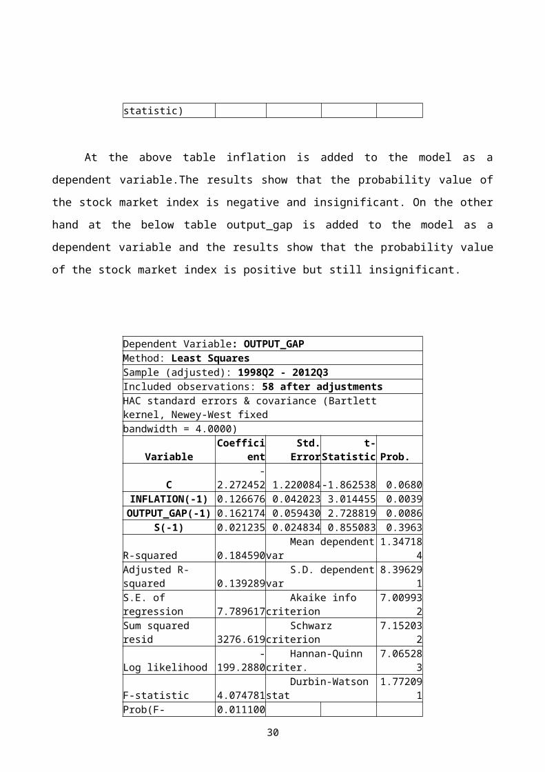
At the above table inflation is added to the model as a
dependent variable.The results show that the probability value of
the stock market index is negative and insignificant. On the other
hand at the below table output_gap is added to the model as a
dependent variable and the results show that the probability value
of the stock market index is positive but still insignificant.
Dependent Variable: OUTPUT_GAPMethod: Least SquaresSample (adjusted): 1998Q2 - 2012Q3Included observations: 58 after adjustmentsHAC standard errors & covariance (Bartlett kernel, Newey-West fixedbandwidth = 4.0000)
VariableCoeffici
entStd.
Errort-
Statistic Prob.
C-
2.272452 1.220084-1.862538 0.0680INFLATION(-1) 0.126676 0.042023 3.014455 0.0039OUTPUT_GAP(-1) 0.162174 0.059430 2.728819 0.0086
S(-1) 0.021235 0.024834 0.855083 0.3963
R-squared 0.184590 Mean dependentvar
1.347184
Adjusted R-squared 0.139289
S.D. dependentvar
8.396291
S.E. of regression 7.789617
Akaike info criterion
7.009932
Sum squared resid 3276.619
Schwarz criterion
7.152032
Log likelihood-
199.2880 Hannan-Quinn criter.
7.065283
F-statistic 4.074781 Durbin-Watson stat
1.772091
Prob(F- 0.011100
30
statistic)
According to the two tables given above the policy rule of
Turkish Central Bank (interest rate) was not affected from the
stock market volatility indirectly.
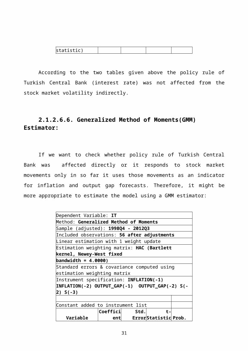
2.1.2.6.6. Generalized Method of Moments(GMM) Estimator:
If we want to check whether policy rule of Turkish Central
Bank was affected directly or it responds to stock market
movements only in so far it uses those movements as an indicator
for inflation and output gap forecasts. Therefore, it might be
more appropriate to estimate the model using a GMM estimator:
Dependent Variable: ITMethod: Generalized Method of MomentsSample (adjusted): 1998Q4 - 2012Q3Included observations: 56 after adjustmentsLinear estimation with 1 weight updateEstimation weighting matrix: HAC (Bartlett kernel, Newey-West fixedbandwidth = 4.0000)Standard errors & covariance computed using estimation weighting matrixInstrument specification: INFLATION(-1) INFLATION(-2) OUTPUT_GAP(-1) OUTPUT_GAP(-2) S(-2) S(-3)
Constant added to instrument list
VariableCoeffici
entStd.
Errort-
Statistic Prob.
31
C 2.844306 0.116867 24.33799 0.0000INFLATION 0.028807 0.003244 8.878953 0.0000
OUTPUT_GAP-
0.003732 0.003913-0.953739 0.3446
S(-1)-
0.000697 0.001029-0.677083 0.5014
R-squared 0.720439 Mean dependentvar
3.457147
Adjusted R-squared 0.704311
S.D. dependentvar
0.545603
S.E. of regression 0.296684
Sum squared resid
4.577116
Durbin-Watson stat 0.170815 J-statistic
4.848948
Instrument rank 7 Prob(J-statistic)
0.183198
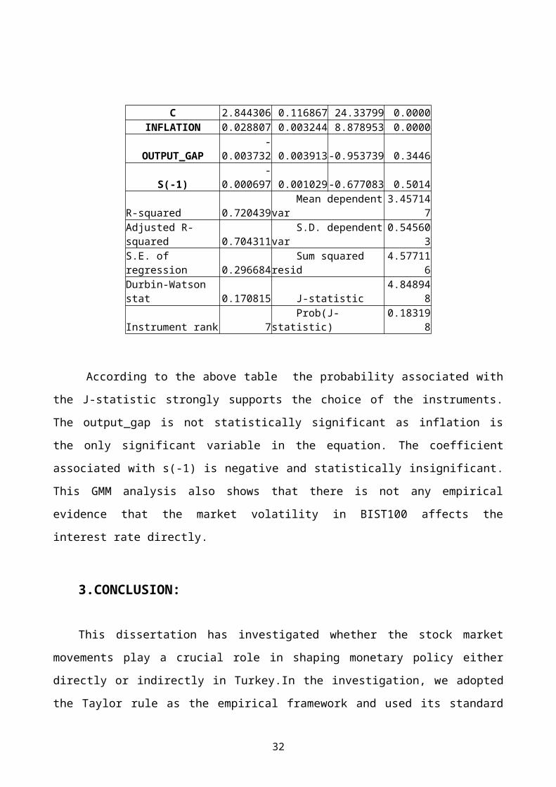
According to the above table the probability associated with
the J-statistic strongly supports the choice of the instruments.
The output_gap is not statistically significant as inflation is
the only significant variable in the equation. The coefficient
associated with s(-1) is negative and statistically insignificant.
This GMM analysis also shows that there is not any empirical
evidence that the market volatility in BIST100 affects the
interest rate directly.
3.CONCLUSION:
This dissertation has investigated whether the stock market
movements play a crucial role in shaping monetary policy either
directly or indirectly in Turkey.In the investigation, we adopted
the Taylor rule as the empirical framework and used its standard
32
and augmented versions in order to reach a conclusion. Right from
the beginning at every stage of the investigation all the tests
results we obtained show that the stock market movements do not
play a crucial role in shaping monetary policy neither directly
nor indirectly in Turkey.
As we mentioned before at previous chapters of our
investigation Turkish economy showed an outstanding performance
between the years of 1997 and 2012.During the period, the
inflation rate dropped to %6.16 from %85 and parallel to the
inflation rate interest rate dropped almost %60 while GDP rose
almost %4 annually in average. Additionally BIST100, the stock
market value of Turkey rose almost 60% in 2012 and reached the
80.000 index level while it was only at 1.613 index level at 1997.
All those macro economic data of Turkey given above and our
test results together show that during our investigation period,
Turkish Central Bank’s policy rule was to achieve and maintain
price stability which is also its primary objective that was given
by the law.The Central Bank of Turkey aimed to achieve and
maintain price stability at the first place while it was also
supporting a sustainable growth and increased employment instead
of supporting the stock market. At the end of the investigation,
we can claim that there is not any empirical evidence that
supports the hypothesis of the stock market movements play a
crucial role in shaping monetary policy directly or indirectly in
Turkey.
33
REFERENCES
Allen, F. and D. Gale (2000), “Bubbles and Crises”, The Economic
Journal, 110, pp. 236-55.
Taylor, John B., (1993). “Discretion Versus Policy Rules in
Practice", Carnegie-Rochester Conference Series on Public Policy 39,pp.195-214
34
Bernanke, B. S. , Mihov, I., (1998). ‘‘Measuring Monetary
Policy’’, The Quarterly Journal of Economics, Vol. 113, No. 3., pp.869-
902.
Bernanke, B. S. , Gertler, M. (2000). “Monetary Policy And Asset
Price Volatility” NBER Working Paper, No. 7559.
Bernanke, B. S. and Gertler, M. (2001). “Should central banks
respond to movements in asset prices?”, American Economic Review,
91(2), pp. 253-257.
Bean, C.R., (2004). “Asset Prices, Financial Instability and
Monetary Policy”, The American Economic Review,Vol. 94, No. 2, pp. 14-18
Bordo, M.D., Jeanne, O. (2002). “Boom-Busts In Asset Prices,
Economic Instability And Monetary Policy” NBER Working Paper, No. 8966
Borsa İstanbul, (2013). Corporate, (online). Available at
http://borsaistanbul.com/en/corporate/about-borsa-istanbul/about-
us, (accesed) 04.08.2013
Castro, V.M.A. (2008) “Are Central Banks following a linear or
nonlinear (augmented) Taylor rule?”, “Working Paper”, University of
Warwick, Department of Economics, Coventry.
35
Cecchetti, S., Genberg, H. and Wadhwani, S. (2002). “Asset Prices
In a Flexible Inflation Targetting Framework”, NBER Working Paper No.
8970.
Engle, R. F. ,(1984).”Wald, Likelihood Ratio, and Lagrange
Multiplier Tests in Econometrics”, Handbook of Econometrics, Volume II,
pp.776-825
Frait, J., Komarek, L., (2006). “Monetary Policy and Asset
Prices,What Role for Central Banks in New EU Member States”,
Warwick Economic Research Papers, No.738
Generalized Method of Moments Estimation, Hansen, L.P., (2007).
(online). Available at http://home.uchicago.edu/.../ Generalized
Method Of Moments (accesed) 02.08.2013
Gilchrist, S., Leahy, J.V., (2002). “Monetary Policy and Asset
Price”, Journal of Monetary Economics,No.49, pp.75-97
Godhart, C., Hofmann, B., (2000). “Do Asset Prices Help to Predict
Consumer Price Index”, The Manchester School Supplement, No.1463-6786,
pp.122-140
Hutcheson, G. D. (2011). “Ordinary Least-Squares Regression”, The
SAGE Dictionary of Quantitative Management Research, Pp.224-228
36
Koichiro Kamada, K. , Muto, I. (2000). “Forward-looking Models
and Monetary Policy in Japan”, Research and Statistic Department, Bank of
Japan, April 2000
Keynes, J. M., (1923). “A tract on monetary reform”, London: Macmillan.
Mavroeidis, S., (2004). “Weak identification of forward-looking
models in monetary economics” Discussion Paper: 2004/06, Department of
Quantitative Economics, University of Amsterdam
Mishkin, F.S. (2012).“The Economics of Money, Banking and Financial Markets”
Global Edition 10. edition, Pearson Education Limited,Harlow,UK
Ozatay, F. , G. Sak (2002). “The 2000-2001 Financial Crisis in
Turkey”, Paper presented at the Currency Crisis Conference of the Brookings
Institution, May 2002, Washington, D.C
SERPAM , (2013). “Türkiye Sermaye Piyasası 2012 Yılı Raporu”,
University of Istanbul SERPAM Research Papers.
37