postprint

Molecular mechanism for azeotropeformation in ethanol/benzene binarymixtures through Gibbs ensembleMonte Carlo simulationLi, Gao, Vasudevan, Li, Gao, Li, and Xi (2020)DOI: 10.1021/acs.jpcb.9b12013 http://xiresearch.org

This document is the accepted manuscript (after peer review) version of an article published in its finalform (i.e., the version of record) by American Chemical Society as

Dongyang Li, Ziqi Gao, Naveen Kumar Vasudevan, Hong Li, Xin Gao, Xingang Li, and Li Xi.Molecular mechanism for azeotrope formation in ethanol/benzene binary mixtures throughGibbs ensemble Monte Carlo simulation. The Journal of Physical Chemistry B, 124:3371–3386, 2020. doi: 10.1021/acs.jpcb.9b12013

(copyright © 2020, American Chemical Society). The version of record is hosted at

https://dx.doi.org/10.1021/acs.jpcb.9b12013

by the publisher.The current version is made available for your personal use only in accordance with the publisher’s

policy. Please refer to the publisher’s site for additional terms of use.

BIBTEX Citation Entry@article{LiJPCB20,author = {Li, Dongyang and Gao, Ziqi and

Vasudevan, Naveen Kumar and Li,Hong and Gao, Xin and Li, Xingangand Xi, Li},

title = {{Molecular mechanismfor azeotrope formation inethanol/benzene binary mixturesthrough Gibbs ensemble Monte Carlosimulation}},

journal= {The Journal of PhysicalChemistry B},

volume = {124},pages = {3371-3386},year = {2020},

}

brought to you by theXI RESEARCH GROUP at McMaster University

www.XIRESEARCH.orgPrinciple Investigator:

Li Xi 奚力Email: li@xiresearch.org

https://twitter.com/xiresearchgrouphttps://linkedin.com/company/xiresearch/https://researchgate.net/profile/Li_Xi16https://mendeley.com/profiles/li-xi11/

A Molecular Mechanism for Azeotrope Formation in

Ethanol/Benzene Binary Mixtures through Gibbs

Ensemble Monte Carlo Simulation

Dongyang Li1,2, Ziqi Gao2, Naveen Kumar Vasudevan2, Hong Li1, Xin Gao∗1,

Xingang Li1, and Li Xi∗2

1School of Chemical Engineering and Technology, National Engineering Research

Center of Distillation Technology, and Collaborative Innovation Center of

Chemical Science and Engineering (Tianjin), Tianjin University, Tianjin 300072,

China2Department of Chemical Engineering, McMaster Universtiy, Hamilton, Ontario

L8S 4L7, Canada

March 19, 2020

∗corresponding authors: gaoxin@tju.edu.cn and xili@mcmaster.ca; URL: http://www.xiresearch.org

1

Abstract

Azeotropes have been studied for decades due to the challenges they impose on

separation processes but fundamental understanding at the molecular level remains

limited. Although molecular simulation has demonstrated its capability of predicting

mixture vapor-liquid equilibrium (VLE) behaviors, including azeotropes, its poten-

tial for mechanistic investigation has not been fully exploited. In this study, we use

the united atom transferable potentials for phase equilibria (TraPPE-UA) force-�eld

to model the ethanol/benzene mixture, which displays a positive azeotrope. Gibbs

ensemble Monte Carlo (GEMC) simulation is performed to predict the VLE phase

diagram, including an azeotrope point. The results accurately agree with experimental

measurements. We argue that the molecular mechanism of azeotrope formation can-

not be fully understood by studying the mixture liquid-state stability at the azeotrope

point alone. Rather, azeotrope occurrence is only a re�ection of the changing relative

volatility between the two components over a much wider composition range. A

thermodynamic criterion is thus proposed based on the comparison of partial excess

Gibbs energy between the components. In the ethanol/benzene system, molecular

energetics shows that with increasing ethanol mole fraction, its volatility initially

decreases but later plateaus, while benzene volatility is initially nearly constant and

only starts to decrease when its mole fraction is low. Analysis of the mixture liquid

structure, including a detailed investigation of ethanol hydrogen-bonding con�gura-

tions at di�erent composition levels, reveals the underlying molecular mechanism for

the changing volatilities responsible for the azeotrope.

2

1 Introduction

Azeotropes are vapor-liquid equilibrium (VLE) states where the compositions are the same

between the two co-existing phases: i.e.,

xi = yi (1)

where xi and yi are repectively the liquid- and vapor-phase mole fractions of component i.

Azeotropes are caused by strong deviation from the ideal-mixture behavior (described by the

Raoult’s law) and their existence poses great challenges for separation processes. Ideal or nearly

ideal mixtures can be clearly di�erentiated according to their volatility based on which separation

can be e�ciently achieved at VLE states using distillation. However, this no longer applies

to azeotropes where volatilities of components are the same. Designing a separation process

for azeotropes always begins with VLE data and a phase diagram, which can be obtained by

experiments1–3 or thermodynamic models (excess Gibbs free energy (gE) models4,5, equations

of state (EoSs)6,7, group contribution methods8,9, etc.). Experiments become di�cult in many

circumstances, such as when toxic chemicals or high pressures are involved, and are commonly

time-consuming and costly. Existing models are typically constructed by empirical or semi-

empirical approaches and apply only to speci�c groups of compounds sharing similar chemical

structures. The lack of generality of those models re�ects our limited understanding of the

molecular origin of the azeotrope phenomenon. Beyond prediction, identifying the molecular

interactions responsible for azeotropes can also help us better design their separation processes,

e.g., through more guided selection of entrainers used in azeotropic distillation.

In a strictly ideal mixture, the intermolecular interactions between unlike molecules equal

those between molecules of the same species and the equilibrium vapor pressure follows the

Raoult’s law, which a for binary mixture writes

P = x1Psat1 (T ) + x2P

sat2 (T ) (2)

3

(P sati is the vapor pressure of pure species i). An azeotrope occurs when strong deviation from

Raoult’s law results in a local minimum or maximum in the vapor pressure versus mole fraction

curve at constant temperature. A vapor pressure minimum is called a negative or maximum

boiling azeotrope, which results from stronger thermodynamic a�nity between di�erent species

in the mixture, making the liquid mixture more stable than the pure species. Likewise, a positive

or minimum boiling azeotrope indicates less favorable interactions and a less stable liquid mixture.

Azeotropes of binary mixtures have been extensively studied over the decades with well established

experimental data sets10–12 and thermodynamic models in the literature (such as Wilson, NRTL,

UNIQUAC, UNIFAC et al.3,13–15). Compared with getting the phase-diagram data, establishing the

molecular mechanism is more di�cult.

Since an azeotrope can be interpreted as either the most (negative azeotrope) or the least

(positive azeotrope) stable liquid mixture, there has been a natural focus on the liquid structure of

the exact azeotrope point. In particular, it is intuitive to speculate the existence of special molecular

arrangements – commonly described as “clusters” – that dominate the liquid azeotropic mixture.

Such clusters are, presumably, formed between di�erent species with stoichiometric ratio and will

be hereinafter referred to as “co-clusters”, which is to be di�erentiated from clusters of molecules

of the same species discussed later in the paper. This concept is especially convenient for negative

azeotropes where clustering between unlike molecules is expected to lead to liquid structures that

are thermodynamically more stable. Experimentally, this concept has been probed with techniques

such as infrared spectroscopy (IR)16,17, mass spectroscopy (MS)18, Raman spectroscopy19, nuclear

magnetic resonance spectroscopy (NMR)20,21, X-ray di�raction22, inelastic neutron spectroscopy19,

and fourier-transform infrared spectroscopy (FT-IR)23,24. In this view, liquid structure at azeotrope

is conceived to be composed of unit co-clusters, each of which has a well-de�ned stoichiometric

ratio between the two types of molecules in the mixture. For example, Jalilian used FT-IR and 1H

NMR to study the acetone/chloroform azeotropic mixture and compared it with pure acetone and

pure chloroform23. They found that the δ(1H) shift occurs at a higher frequency in the azeotrope

than it does in pure acetone or chloroform, which was considered a sign for the formation of

4

acetone-chloroform molecular co-clusters. The proposed unit structure contains two chloroform

molecules connected with one acetone molecule by two type of hydrogen bonds (HBs) – one

between the hydrogen in chloroform and the oxygen in acetone, and the other between one methyl

hydrogen of acetone and one chlorine in chloroform. A number of other azeotropic systems, such

as acetone/n-pentane25, methanol/benzene26, acetone/cyclopentane27, and acetone/cyclohexane28,

were similarly studied. Without direct molecular images of such unit co-clusters, their structures

were commonly deduced from the number and type of available hydrogen-bond binding sites

of both molecules. Theoretical arguments can also be made through, e.g., the density functional

theory (DFT) which calculates the potential energy of pre-speci�ed unit co-cluster con�gurations.

Ripoll et al. 29 performed DFT calculation on co-clusters of water/diethyl carbonate (DEC) at

di�erent stoichiometric ratios and found that the one with a 3:1 ratio is most stable, which

agrees with the experimentally measured xwater ≈ 0.75 at the azeotrope. Similar calculations were

reported for methanol/benzene30, ethanol/isooctane31, hydrogen �uoride/water32, ethanol/water33,

etc.

Despite its apparent appeal, especially in terms of explaining the azeotropic composition based

on the stoichiometric ratio in the unit co-clusters, limitations of this idea are also evident. The

concept of a unit co-cluster at the azeotropic composition being energetically favorable resonates

with that of a unit cell in a cocrystal structure, except that the mixture here is fundamentally

still a liquid – local composition �uctuations would constantly disturb any ordered co-clusters

should they ever emerge. As such, the concept of co-clusters is not well-de�ned and is hard to

verify in real disordered liquid structures. Indeed, direct evidence for ordered co-cluster structures

with a clear stoichiometric ratio of the two components has not been found. Meanwhile, the

proposed existence of such co-clusters would only explain the relative thermodynamic stability

of the azeotropic composition (and from an energetic argument only) and thus its lower vapor

pressure compared with the ideal mixture limit, which, by itself, is a necessary condition for

negative azeotrope but not a su�cient one. It would also struggle to explain a positive azeotrope

where the unit co-clusters would have to be less stable than a completely random mixture.

5

Recently, Shephard et al. 34 reported a detailed investigation of the liquid structure at the

azeotropic composition for both a positive (methanol/benzene) and negative (acetone/chloro-

form) azeotrope system with neutron scattering and the di�raction data were converted to a

detailed molecular representation with the empirical potential structure re�nement (EPSR) mod-

eling approach35,36 (which �ts the molecular model to di�raction data with a Monte Carlo –

MC – algorithm). Clear di�erences were found in the structural patterns of these two types

of azeotropes. For methanol/benzene, strong association is found between methanol molecules.

Inserting benzene molecules at the azeotropic composition does not lead to the formation of binary

co-clusters proclaimed by the co-cluster theory. Rather, clustering still occurs between methanol

molecules and benzene molecules are largely left out of methanol-rich regions. Meanwhile, for

acetone/chloroform, the two components interact through both HB (acetone-O and chloroform-H)

and halogen-bond (acetone-O and chloroform-Cl) interactions, which leads to a moderate increase

of cross-species association at the azeotrope compared with a random mixture and explains its

relative stability. However, clear ordered co-clusters are still absent.

We note that the de�ning di�erence between an azeotropic mixture and a general non-ideal one

is whether the relative volatilities of the two components switch places. In a non-azeotropic mixture

(ideal or non-ideal), the component with higher vapor pressure in its pure form is consistently

more volatile in the mixture for the entire composition range, whereas in an azeotropic mixture,

the component more volatile before the azeotrope becomes less volatile after the azeotrope. A

molecular mechanism for azeotrope will have to explain this transition, which requires us to go

beyond the azeotropic point and examine the entire range of composition. Fewer experimental

e�orts have been reported on this front. Akihiro Wakisaka37–39 used mass spectroscopy to analyze

and compare the patterns of molecular organization in an ethanol/water mixture before and after

the azeotrope. They proposed that at lower xethanol, the liquid structure is dominated by strong

water-water hydrogen-bonding interactions and thus ethanol is more volatile. At higher xethanol

the scenario is reversed and thus water becomes more volatile. This argument, of course, only

applies to mixtures of two polar components each with strong self interactions.

6

Molecular simulation provides direct access into the microscopic molecular structures and

detailed intermolecular interactions that are only inferred indirectly in experiments. It has been

widely used in the study of liquid thermodynamics for the prediction of their phase behaviors

and thermodynamic properties and for fundamental inquiries into the underlying molecular

mechanisms40–42. For azeotrope research, however, previous e�orts mostly focused on its predic-

tion as well as the prediction of the VLE phase diagram. The potential of molecular simulation

for its mechanistic understanding has not been fully exploited. Azeotropes were captured in

molecular simulation as early as the study of the carbon dioxide/ethane system using a Lennard-

Jones (L-J) model by Scalise et al. 43 . Several simulation techniques have since been applied to

azeotrope research. One example is the Gibbs Duhem integration (GDI) method44, which was

successfully applied by Pandit and Kofke45 to capture azeotropes modeled by di�erent L-J model

parameters. Its accuracy for phase equilibrium prediction depends strongly on the initial condi-

tion for integration46,47 and it also fails to capture the critical-point phenomenon44,45,48. Another

method is histogram-reweighting Monte Carlo (HrMC)49 which accurately predicts the location

of azeotropic points in ethane/per�uoroethane, propanal/n-pentane, and acetone/n-hexane mix-

tures50,51. However, for many other mixtures, such as acetone/chloroform, acetone/methanol,

and chloroform/methanol, azeotrope prediction by HrMC was found to be rather inaccurate52.

The most widely used method in this area is the Gibbs ensemble Monte Carlo (GEMC) method40

which has been applied to the VLE of a wide range of azeotropic mixtures, such as ethanol/wa-

ter53, methanol/n-hexane54, ethanol/n-hexane54, 1-pentanol/n-hexane55, methanol/acetonitrile56,

1-propanol/acetonitrile55, ethyl acetate/ethanol57, and methanol/ethyl acetate57. The success of

the GEMC approach established an e�cient and reliable way for predicting azeotropes given

su�ciently accurate force-�eld parameters for the molecules involved.

Overall, although azeotrope is a well-known thermodynamic phenomenon of much practical

signi�cance, fundamental understanding into its molecular origin is rather limited. There has

been a historical emphasis on explaining its existence through its strong departure from the ideal

mixture behavior, which has led to a focus on the liquid structure at the azeotropic composition.

7

Many of those e�orts were targeted at identifying the molecular arrangement, often conjectured

to be co-clusters formed by di�erent species with stoichiometric ratio, responsible for the raised

or reduced volatility (vapor pressure) compared with the Raoult’s law. We will instead focus on

the qualitative feature that distinguishes azeotropic mixtures from non-azeotropic ones – the

changing relative volatility between components. In this study, a thermodynamic criterion for the

occurrence of azeotrope is developed based on this perspective and used as the guidance for its

molecular understanding. GEMC simulation is performed on the ethanol/benzene system as a

representative example of positive azeotrope formed by a polar/non-polar pair. The full VLE phase

diagram is successfully reproduced in our simulation including the occurrence of an azeotrope,

which to our knowledge has not be reported before for this system. Molecular interactions are

analyzed according to the thermodynamic criterion. Changes in molecular energetics are then

traced back to the changing liquid-phase structure for the entire composition range. It is revealed

that at di�erent compositions, the molecular arrangement undergoes transitions between distinct

stages, which explains the changing thermodynamic properties and eventually the occurrence

of an azeotrope. This is to our knowledge the �rst in-depth investigation, based on molecular

simulation, into the molecular mechanism for azeotrope formation that connects the microscopic

liquid structure to macroscopic thermodynamics. The molecular mechanism proposed here is

expected to be generalizable for other positive azeotropes in binary mixtures between polar and

non-polar species.

2 Simulation details

The TraPPE-UA (Transferable Potentials for Phase Equilibria - United Atoms) force �eld58,59 is

applied to model ethanol and benzene molecules. This is a united-atom (UA) model in which the H

atoms in CH3, CH2, and aromatic CH(aro) are grouped with their host C as bundled pseudo-atoms,

whereas the hydroxyl H is modeled as a separate point charge. The pairwise-additive L-J 12-6

potential combined with Coulombic interactions between partial charges is used to describe

8

non-bonded interactions

unon-bonded(rij) = 4εij

[(σijrij

)12

−(σijrij

)6]

+qiqj

4πε0rij(3)

where ε0 is the vacuum permittivity, i and j are atom indices, qi and qj are the partial charges

of atoms i and j, rij , εij , and σij are their separation distance, LJ energy well depth, and LJ

length scale, respectively. The Lorentz-Berthelot combination rule60,61 is used to determine the

cross-interaction LJ parameters between unlike atoms

σij = (σii + σjj)/2 (4)

εij =√εiiεjj. (5)

A cuto� of 14 Å was applied to the non-bonded pairwise interactions with an analytical tail

correction to minimize the truncation error in the LJ interaction62,63. The Ewald summation with

a tin-foil boundary condition was used to calculate the long-range electrostatic potential62 using

the same settings as Wick et al. 64 and Chen et al. 54 .

In the TraPPE-UA force �eld, all bond lengths are �xed, but a harmonic potential is used to

describe the bending resistance of bond angles

ubend =kθ2 (θ − θ0)

2 (6)

where θ, θ0, and kθ are the measured bond angle, the equilibrium bending angle, and the force

constant, respectively. Meanwhile, a torsion potential is applied to control the dihedral rotation

around bonds,

utors = c0 + c1[1 + cos(φ)] + c2[1− cos(2φ)] + c3[1 + cos(3φ)] (7)

where c0, c1, c2, and c3 are the dihedral interaction coe�cients and φ is the dihedral angle. All

9

Table 1: Non-bonded interaction parameters for ethanol and benzene in the TraPPE-UA force�eld54,64.

(Pseudo-)Atom molecule σ [Å] ε/kB [K] q[e]CH3 ethanol 3.750 98CH2 ethanol 3.950 46 +0.265

CH(aro) benzene 3.695 50.5O ethanol 3.020 93.0 -0.700

H (in OH) ethanol +0.435(Note: kB is the Boltzmann constant.)

Table 2: Bonded interaction parameters for ethanol and benzene in the TraPPE-UA force �eld54,64.

Bond Length r0 [Å]CH3-CH2 1.540

CH2-O 1.430O-H 0.945

CH(aro)-CH(aro) 1.400

Bond Angle θ0 [deg.] kθ/kB [K]CH3-CH2-O 109.47 50400CH2-O-H 108.50 55400

CH(aro)-CH(aro)-CH(aro) 120.00 rigid

Torsion Angle c0/kB [K] c1/kB [K] c2/kB [K] c3/kB [K]CH3-CH2-O-H 0 209.82 -29.17 187.93

non-bonded and bonded potential parameters are taken from references54,64 and are listed in

table 1 and table 2.

Constant-temperature constant-pressure GEMC simulation, involving coupled-decoupled

con�gurational-bias Monte Carlo (CBMC) sampling moves65,66, was employed to compute the VLE

of ethanol/benzene mixtures at 15 composition levels (hereinafter, liquid-phase mole fractions are

denoted by xi, where i = 1 for ethanol and i = 2 for benzene). The simulation pressure was set to

1 atm for all compositions (which means the temperature of VLE varies). The total number of these

two types of molecules were controlled at 450 and these molecules were initially allocated between

the two simulation cells – one for the liquid phase and one for the vapor phase – at random. In

10

0.0 0.2 0.4 0.6 0.8 1.0x1(y1)

340

343

346

349

T (K

)

x1, exp

y1, exp

x1, sim

y1, sim

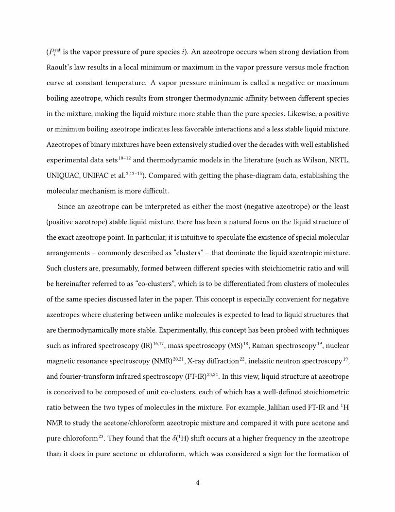
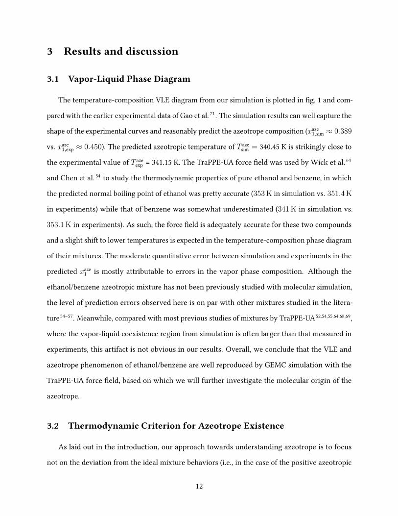
Figure 1: Comparison of the vapor-liquid equilibrium (VLE) phase diagram (1atm) from oursimulation (circles) with the experiments of Gao et al. 71 (triangles): 1–ethanol, 2–benzene. (Error

bars are smaller than the marker size and thus not shown.)

either cell, molecules were placed on a cubic lattice in the initial con�guration. For each simulation,

80000 MC cycles were used to equilibrate the system, followed by another 30000 cycles for the

production run. Each cycle contains 450 MC moves. Both the initial con�guration generation and

the GEMC simulation were performed using the MCCCS Towhee program58,59. The converged

liquid cell has a dimension of approximately 30× 30× 30Å3. The block averaging approach was

used for uncertainty analysis67: the production run was divided into �ve equal blocks and the

standard error between the block averages is reported as the simulation uncertainty. Five types

of MC moves were used in the sampling54,55,58,64,68–70: volume exchanges and CBMC molecular

swaps between the two cells, CBMC conformational bias moves, and molecular translations and

rotations. Each MC move was randomly selected with a 0.1-1% probability for volume exchange

and 20-30% for molecule swap moves; the remaining probability was evenly divided between

conformation bias moves, translations, and rotations.

11

3 Results and discussion

3.1 Vapor-Liquid Phase Diagram

The temperature-composition VLE diagram from our simulation is plotted in �g. 1 and com-

pared with the earlier experimental data of Gao et al. 71 . The simulation results can well capture the

shape of the experimental curves and reasonably predict the azeotrope composition (xaze1,sim ≈ 0.389

vs. xaze1,exp ≈ 0.450). The predicted azeotropic temperature of T aze

sim = 340.45 K is strikingly close to

the experimental value of T azeexp = 341.15 K. The TraPPE-UA force �eld was used by Wick et al. 64

and Chen et al. 54 to study the thermodynamic properties of pure ethanol and benzene, in which

the predicted normal boiling point of ethanol was pretty accurate (353 K in simulation vs. 351.4 K

in experiments) while that of benzene was somewhat underestimated (341 K in simulation vs.

353.1 K in experiments). As such, the force �eld is adequately accurate for these two compounds

and a slight shift to lower temperatures is expected in the temperature-composition phase diagram

of their mixtures. The moderate quantitative error between simulation and experiments in the

predicted xaze1 is mostly attributable to errors in the vapor phase composition. Although the

ethanol/benzene azeotropic mixture has not been previously studied with molecular simulation,

the level of prediction errors observed here is on par with other mixtures studied in the litera-

ture54–57. Meanwhile, compared with most previous studies of mixtures by TraPPE-UA52,54,55,64,68,69,

where the vapor-liquid coexistence region from simulation is often larger than that measured in

experiments, this artifact is not obvious in our results. Overall, we conclude that the VLE and

azeotrope phenomenon of ethanol/benzene are well reproduced by GEMC simulation with the

TraPPE-UA force �eld, based on which we will further investigate the molecular origin of the

azeotrope.

3.2 Thermodynamic Criterion for Azeotrope Existence

As laid out in the introduction, our approach towards understanding azeotrope is to focus

not on the deviation from the ideal mixture behaviors (i.e., in the case of the positive azeotropic

12

system of ethanol/benzene, its lower boiling point compared with the Raoult’s law), but on the

changing relative volatility between the two components before and after the azeotrope. In our

current system (�g. 1), at x1 < xaze1 , ethanol remains the more volatile component (i.e., at given

temperature, ethanol’s mole fraction in the liquid phase x1 is lower than that in its coexisting

vapor phase y1), but after the azeotrope, benzene takes over and has a higher tendency to vaporize

(x1 > y1). Our goal is to reveal the molecular origin behind this switch of relative volatility, which

only occurs at the azeotrope. Note that azeotropes can occur even when the vapor phase is an

ideal gas. At ambient pressure studied here, it is a phenomenon solely driven by liquid-phase

mixture thermodynamics. Therefore, we focus on the changes in the thermodynamic properties

and molecular arrangement, before and after the azeotrope, in the liquid phase only.

We start from the fundamental criterion for azeotropes and derive the corresponding relations

in terms of the thermodynamic properties of azeotropic mixtures. When a binary azeotrope

appears, the composition of the liquid phase is equal to that of the vapor phase (eq. (1)). Assuming

ideal gas for the vapor phase, the equilibrium compositions are related through the modi�ed

Raoult’s law

y1P = x1γ1Psat1 (8)

y2P = x2γ2Psat2 . (9)

Combining these two equations, the relationship between the activity coe�cients, γi, and the

corresponding vapor pressure of the pure species, P sati , is written to be

γ1

γ2=

(y1

x1

)(x2

y2

)P sat

2P sat

1. (10)

At the azeotrope, eq. (1) is invoked. Taking logarithm of both sides, we get

lnP sat

2P sat

1= ln

γ1

γ2= ln γ1 − ln γ2 =

GE1

RT− GE

2RT

(when x1 = xaze1 ) (11)

13

where the last equality comes from the thermodynamic relation,

GEi = RT ln γi, (12)

GEi is the partial excess Gibbs free energy of component i (the overbar denotes partial molar

properties and superscript “E” represents excess properties – i.e., departure from the ideal mixture),

and R is the ideal gas constant. For a positive azeotrope, before the azeotropic point, x1 < y1 and

y2 < x2, and after the azeotropic point, x1 > y1 and y2 > x2. Therefore, the relationship between

P sati and GE

i is as follows:

GE

1RT− GE

2RT

> lnP sat

2P sat

1(when x1 < xaze

1 )

GE1

RT− GE

2RT

< lnP sat

2P sat

1(when x1 > xaze

1 )

(13)

where P sati can be easily estimated with the Antoine equation72

lnPisat = Ai −

Bi

Ci + T(14)

at the targeted temperatures (Ai, Bi, and Ci are species-speci�c parameters). GEi is calculated

from its de�nition

GEi ≡ Gi −Gid

i (15)

where Gi is the partial molar Gibbs free energy (i.e., chemical potential) directly collected from

the GEMC simulations. Its counterpart in an ideal mixture can also be calculated –

Gidi = Gi +RT lnxi (16)

– in which the pure-species molar Gibbs free energy Gi is computed by building and equilibrating

a pure liquid cell of species i54,64.

14

0.0 0.2 0.4 0.6 0.8 1.0x1

3

2

1

0

1

2

3

Norm

alize

d Fr

ee E

nerg

y

ln(Psat2 /Psat

1 )(GE

1 GE2)/RT

GE1/RT

GE2/RT

Figure 2: Partial excess Gibbs free energy analysis of the ethanol/benzene liquid mixture at VLE(see eqs. (11) and (13) and related discussion): 1 – ethanol, 2 – benzene. (Error bars smaller than

the marker size are not shown.)

The most important takeaway from eqs. (11) and (13) is that azeotrope is marked by a crossover

between the (GE1 − GE

2)/(RT ) vs. x1 and ln(P sat2 /P sat

1 ) vs. x1 lines. For the benzene/ethanol

system studied, these two quantities are calculated and plotted in �g. 2 for the entire composition

range. The vapor pressure ratio of the two species is not sensitive to temperature, at least within

the range of the VLE phase diagram – ln(P sat2 /P sat

1 ) is nearly a �at line. Meanwhile, the partial

excess Gibbs free energy di�erence between ethanol and benzene, (GE1 − GE

2)/(RT ), decreases

monotonically: it starts above the ln(P sat2 /P sat

1 ) line (i.e., component 1 – ethanol – is more volatile)

and steadily declines with increasing x1 and intersects with the latter at around x1 = 0.4, which

matches the azeotrope point. This simply con�rms the thermodynamic argument of eqs. (11)

and (13). In cases with negative azeotropes, the crossover would still take place but in an opposite

direction: (GE1 − GE

2)/(RT ) would rise from below ln(P sat2 /P sat

1 ) and exceed the latter at the

azeotrope. Meanwhile, for non-azeotropic systems, if (GE1 − GE

2)/(RT ) is initially higher than

ln(P sat2 /P sat

1 ), it would stay so for the entire composition range, and vice versa.

The key of understanding azeotrope formation lies thus in the molecular origin for the drastic

changes in the relative magnitudes of GE1 and GE

2. Partial excess Gibbs free energies of the two

15

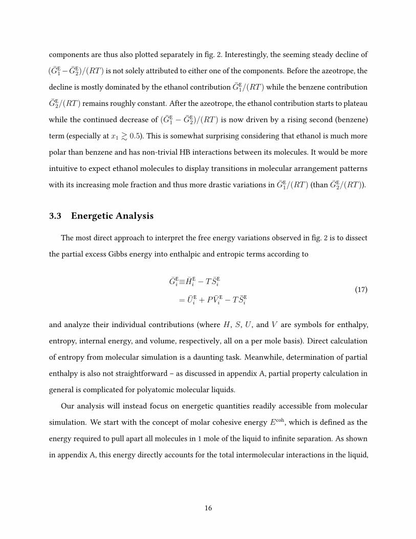
components are thus also plotted separately in �g. 2. Interestingly, the seeming steady decline of

(GE1− GE

2)/(RT ) is not solely attributed to either one of the components. Before the azeotrope, the

decline is mostly dominated by the ethanol contribution GE1/(RT ) while the benzene contribution

GE2/(RT ) remains roughly constant. After the azeotrope, the ethanol contribution starts to plateau

while the continued decrease of (GE1 − GE

2)/(RT ) is now driven by a rising second (benzene)

term (especially at x1 & 0.5). This is somewhat surprising considering that ethanol is much more

polar than benzene and has non-trivial HB interactions between its molecules. It would be more

intuitive to expect ethanol molecules to display transitions in molecular arrangement patterns

with its increasing mole fraction and thus more drastic variations in GE1/(RT ) (than GE

2/(RT )).

3.3 Energetic Analysis

The most direct approach to interpret the free energy variations observed in �g. 2 is to dissect

the partial excess Gibbs energy into enthalpic and entropic terms according to

GEi≡HE

i − T SEi

= UEi + PV E

i − T SEi

(17)

and analyze their individual contributions (where H , S, U , and V are symbols for enthalpy,

entropy, internal energy, and volume, respectively, all on a per mole basis). Direct calculation

of entropy from molecular simulation is a daunting task. Meanwhile, determination of partial

enthalpy is also not straightforward – as discussed in appendix A, partial property calculation in

general is complicated for polyatomic molecular liquids.

Our analysis will instead focus on energetic quantities readily accessible from molecular

simulation. We start with the concept of molar cohesive energy Ecoh, which is de�ned as the

energy required to pull apart all molecules in 1 mole of the liquid to in�nite separation. As shown

in appendix A, this energy directly accounts for the total intermolecular interactions in the liquid,

16

which must be broken to separate the molecules: i.e.

Ecoh ≈ −E inter. (18)

The minus sign is because cohesive energy is de�ned based on the liquid as the reference state

– it is the energy change from the bulk liquid phase to a hypothesized state where molecules

are isolated from one another (eq. (25) in appendix A). When intermolecular interactions are

more attractive (lower E inter), separating the molecules would cost more energy (higher Ecoh).

Contributions to the cohesive energy are attributable to each constituting component through a

quantity we de�ne as (for the lack of a better term) binding energy. The molar binding energy of

component 1 Ebind1 , for example, describes the energy required to strip individual component-1

molecules from the liquid to in�nite distance, scaled to the per mole (of component 1) basis,

while keeping the remaining molecules unmoved. This hypothetical process only breaks the

intermolecular interactions between the removed molecule and all other molecules in the liquid.

Binding energy is related to cohesive energy via

Ecoh =1

2

(x1E

bind1 + x2E

bind2

)(19)

as shown also in appendix A (eq. (34)).

We postulate that component free energy variations in �g. 2 are dominated by binding energy

changes, which means −Ebindi would capture major trends in the GE

i pro�les, even although their

magnitudes may not be directly comparable. (The minus sign, again, is because binding energy is

de�ned with the liquid state as the reference state.) According to eq. (17), three assumptions are

implied in our approach.

1. Contribution by entropy change is secondary, which is not to say that −T SEi must be small,

but assume that its variation between di�erent mixture composition is smaller than that of

the enthalpy term.

2. Within enthalpy, contribution of the PV Ei term is much smaller than that of energy.

17

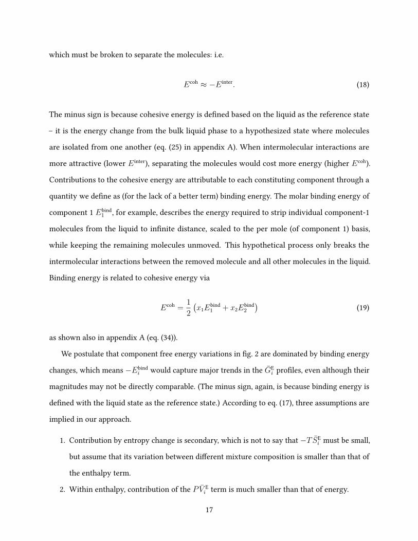
Figure 3: Breakdown of the cohesive energy of the ethanol-benzene liquid mixture at VLE andbinding energies of the components: (a) contributions to the binding energy (see eqs. (32)

and (33)) and (b) contributions to cohesive energy (see eq. (34)). (Error bars smaller than themarker size are not all shown.)

3. Energy change associated with mixing, which is quanti�ed by UEi , is dominated by the

changing intermolecular interactions, which means its major trends will be captured by

−Ebindi .

The �rst assumption is proposed considering the strong polar-polar interactions between ethanol

molecules. Mixing ethanol with benzene disrupts those interactions and this change is expected

to be large. Although entropy change of mixing is substantial, eq. (17) only concerns excess

entropy, which measures the deviation from the ideal mixing case. Therefore, variation of the

T SEi term is small as long as the entropy change deviates from the ideal mixing limit to a similar

extent at di�erent composition. The second assumption is a safe one for liquids near ambient

conditions, where the PV term is generally much smaller than U in enthalpy. The last assumption

is also plausible. For simple molecules like ethanol or benzene, mixing does not cause substantial

molecular conformational change – thus, change in intramolecular energy is expected to be small.

The whole idea can also be intuitively rationalized: when a molecule of component i feels stronger

pulling from other molecules in the mixture, Ebindi is higher, Ei is lower (lower energy corresponds

to more favorable interactions), Gi is lower, and component i is less volatile.

Validity of these assumptions can only be tested by comparing the GEi pro�les in �g. 2 with

those of binding energy. The composition dependence of cohesive and binding energies of the

18

liquid mixture at VLE is calculated and plotted in �g. 3(a). Overall, Ecoh slowly but steadily

increases with x1, which is expected because as the mixture becomes more polar with a higher

portion of ethanol, the molecules are harder to be broken apart. By contrast, the binding energies

of individual components do not share the same monotonic trend. For ethanol, Ebind1 initially

increases but saturates to a plateau at medium to high x1 regions. This is consistent with the

GE1 pro�le in �g. 2, which initially declines but later converges to a nearly �at line. The turning

point observed here (Ebind1 ) occurs at a somewhat lower x1 value than that of GE

1, which may be

attributed to the di�erences between these two quantities such as the entropy component in GEi .

Similarly for benzene, Ebind2 is initially in a plateau but starts to decrease at x1 ≈ 0.5 (shortly after

the azeotrope point at xaze1 = 0.389), which closely re�ects the trend of GE

2 in �g. 2.

It is clear that binding energy pro�les of the components capture the most important trends in

partial excess Gibbs energy, suggesting that the formation of the azeotrope, driven by the variation

of (GE1 − GE

2)/(RT ), can be explained from an energetic argument. In particular, �g. 2 showed

that, somewhat unexpectedly, the change of relative volatility between the two components over

di�erent compositions has two separate driving mechanisms: (1) the initial decrease of ethanol

volatility (decrease of GE1 at small x1), which corresponds to the increases in its binding energy

Ebind1 ; and (2), after the GE

1 and Ebind1 plateau, the continued shift of volatility is overtaken by the

increasing volatility of benzene GE2 and its lowering binding energy Ebind

2 .

Binding energy is further broken down to contributions from self- and cross-interactions

Ebind1 = Ebind

11 + Ebind12 (20)

Ebind2 = Ebind

22 + Ebind21 (21)

(detailed mathematical de�nitions are given in eqs. (32) and (33) in appendix A), which is also

shown in �g. 3(a). The initial high-slope increase of Ebind1 is mainly driven by the interaction with

other type 1 (ethanol) molecules – i.e., the Ebind11 term, which is expected because of the strong

polar-polar (such as HB) interactions. The increase in Ebind11 , however, slows down after x1 ≈ 0.2,

19

marking the end of the �rst driving mechanism discussed above. Meanwhile, the ethanol-benzene

interaction contribution Ebind12 decreases monotonically, roughly proportional to the decreasing

mole fraction of benzene. Its slope is small compared with the initial rapid rise in Ebind11 but is

su�cient to o�set the slower ramp in the latter after x1 ≈ 0.2, resulting in the plateau in the overall

Ebind1 . For benzene, the initial plateau ofEbind

2 also results from the compensation of the decreasing

self-interaction Ebind22 by the increasing cross-interaction with ethanol Ebind

21 . Indeed, the Ebind22

pro�le is nearly parallel to the Ebind12 one in that regime as both drop as a result of having fewer

benzene molecules around. At x1 & 0.5, the drop of Ebind22 takes a sharper slope, indicating that the

arrangement of benzene molecules has fundamentally changed and the lowering self-interaction

can no longer be solely accounted for by the decreasing percentage of benzene in the mixture.

This leads to the overall decline of Ebind2 and, eventually, of GE

2.

Finally, �g. 3(b) shows the breakdown of the cohesive energy into binding energy of compo-

nents according to eq. (19): Ecoh is clearly the sum of x1Ebind1 /2 and x2Ebind

2 /2 over the entire

composition range. The dashed lines show the component contributions to the cohesive energy

if the self-interaction terms – x1Ebind11 /2 and x2Ebind

22 /2 – are considered alone (i.e., neglecting

cross-interaction contributions). Comparison with the solid lines shows that cross-interactions

between di�erent species contribute a very low proportion to the total cohesive energy. We

may also see from �g. 3(a) that Ebind12 is signi�cantly lower than Ebind

11 for the entire composition

range, whereas Ebind21 is lower than Ebind

22 until x1 & 0.7. Dominance of self-interaction in both

components suggests that ethanol (1) and benzene (2) molecules are not uniformly distributed

across the space. Ethanol molecules are much more likely to closely interact with other ethanol

molecules for all x1 levels while benzene molecules also tend to group with their own kind until

their mole fraction x2 is very low.

3.4 Micro-Structure Analysis

We now analyze the microscopic origin, in terms of molecular arrangement patterns, for the

energetic variations responsible for the azeotrope. Although the gathering of ethanol molecules is

20

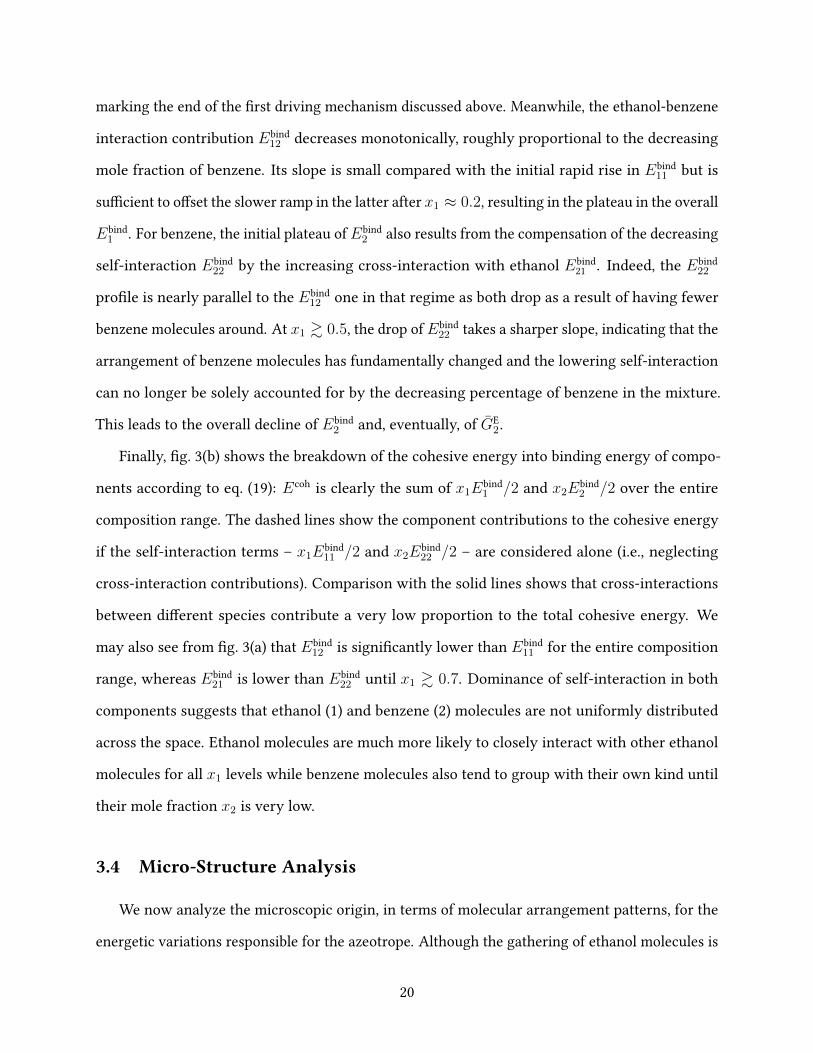
（a）

Figure 4: Arrangement of hydroxyl H atoms around hydroxyl O atoms between ethanol molecules(i.e., atom pairs belonging to the same OH group are excluded) in the liquid phase at VLE: (a)

radial distribution function (RDF; lower pro�les correspond to higher x1); (b) coordinationnumber (CN; rvalley = 2.45 Å). (In (b), error bars smaller than the marker size are not shown.)

very much expected due to their strong polarity and mutual interaction, strong binding between

them would only predict a continuous decrease of ethanol volatility. We have already shown

that the azeotrope occurs as a combined outcome of the lowering ethanol volatility at low x1 and

raised benzene volatility at high x1. The plateauing of Ebind1 and the decay of Ebind

2 at medium to

high x1 regimes are not explained by this naive picture considering ethanol-ethanol interaction

alone.

3.4.1 Molecular Organization

We start with the radial distribution function (RDF) g(r) between the oxygen atom in ethanol

and the hydroxyl hydrogen of a di�erent ethanol molecule in �g. 4(a). It measures the average

number density of hydroxyl H at distance r from a hydroxyl O with which it does not share a

bond, normalized by the domain-average number density of hydroxyl H. In all pro�les, a clear

peak is found at r ≈ 1.8 Å, the typical length of a HB73,74. It is followed by a secondary peak at

around r ≈ 3.4 Å, likely from another ethanol molecule connected to the pair through consecutive

HB interactions. Formation of small clusters of ethanol molecules in the non-polar solvent of

benzene is very much expected. What is surprising, however, is that the peak amplitude decreases

with increasing ethanol mole fraction x1. Indeed, except the lowest mole fraction level x1 = 0.008

21

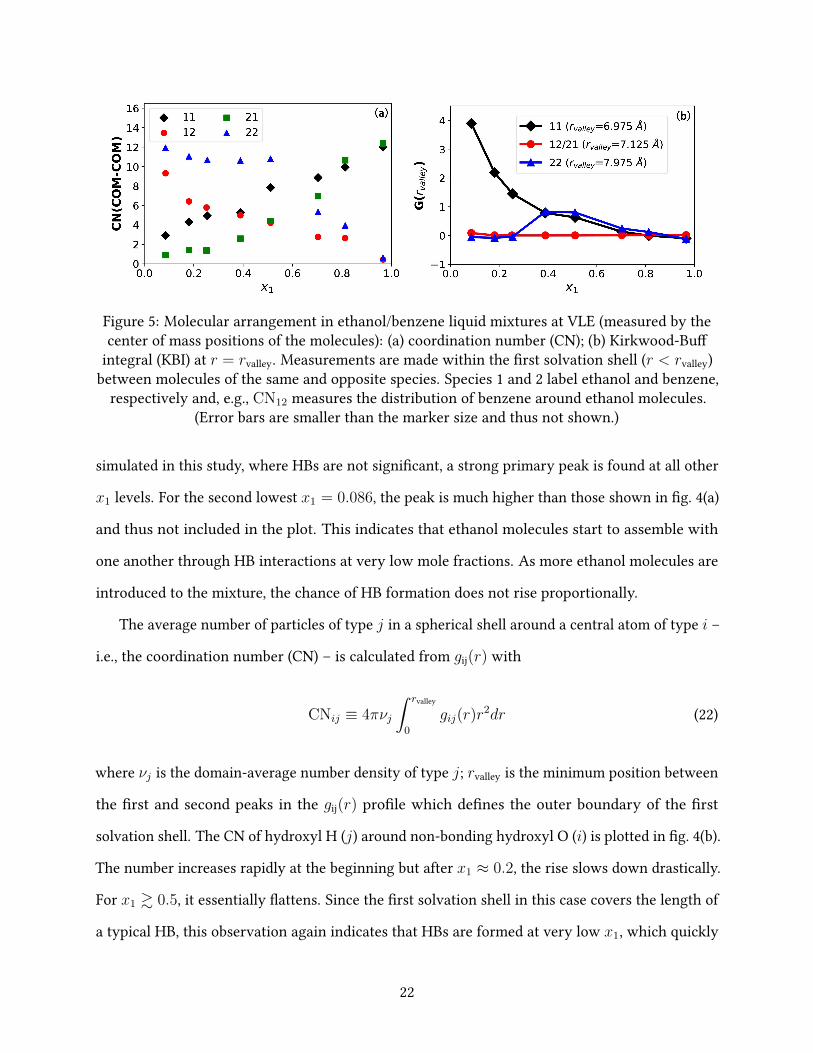
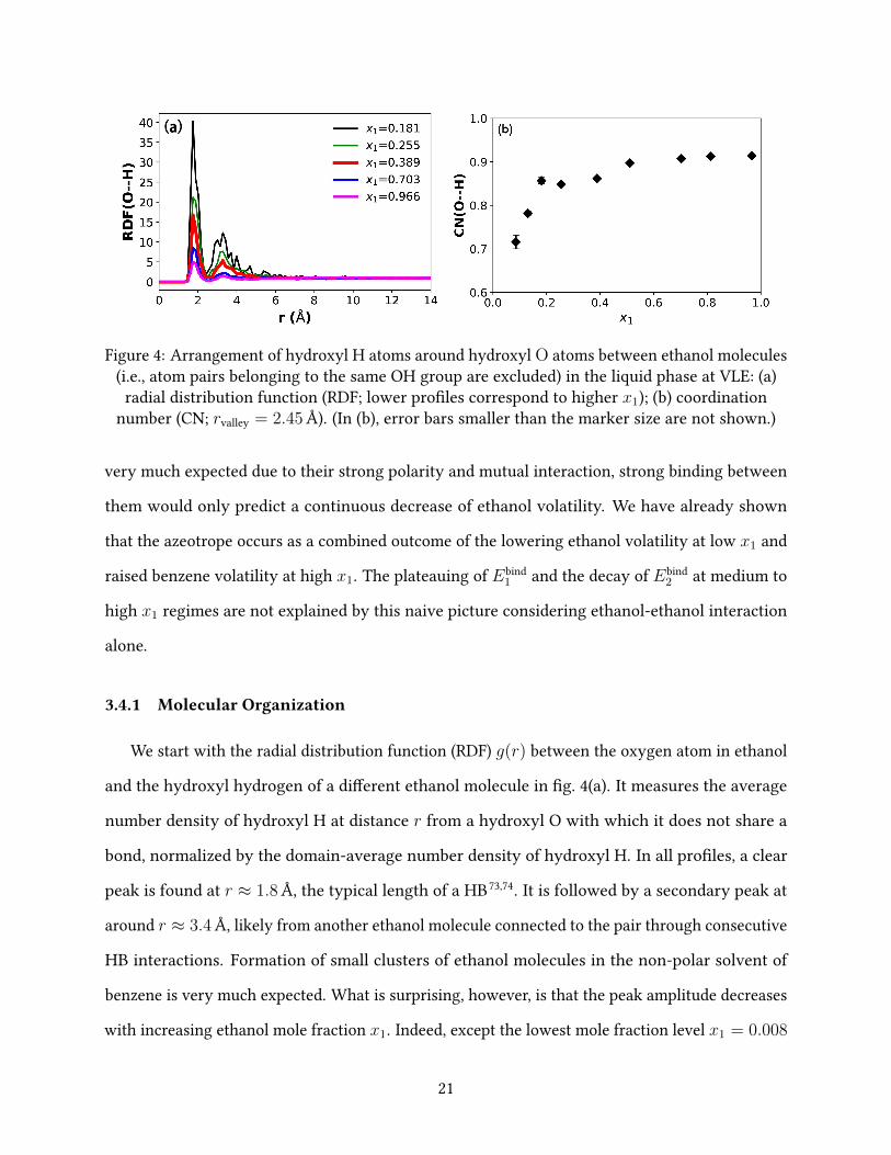
Figure 5: Molecular arrangement in ethanol/benzene liquid mixtures at VLE (measured by thecenter of mass positions of the molecules): (a) coordination number (CN); (b) Kirkwood-Bu�

integral (KBI) at r = rvalley. Measurements are made within the �rst solvation shell (r < rvalley)between molecules of the same and opposite species. Species 1 and 2 label ethanol and benzene,

respectively and, e.g., CN12 measures the distribution of benzene around ethanol molecules.(Error bars are smaller than the marker size and thus not shown.)

simulated in this study, where HBs are not signi�cant, a strong primary peak is found at all other

x1 levels. For the second lowest x1 = 0.086, the peak is much higher than those shown in �g. 4(a)

and thus not included in the plot. This indicates that ethanol molecules start to assemble with

one another through HB interactions at very low mole fractions. As more ethanol molecules are

introduced to the mixture, the chance of HB formation does not rise proportionally.

The average number of particles of type j in a spherical shell around a central atom of type i –

i.e., the coordination number (CN) – is calculated from gij(r) with

CNij ≡ 4πνj

∫ rvalley

0

gij(r)r2dr (22)

where νj is the domain-average number density of type j; rvalley is the minimum position between

the �rst and second peaks in the gij(r) pro�le which de�nes the outer boundary of the �rst

solvation shell. The CN of hydroxyl H (j) around non-bonding hydroxyl O (i) is plotted in �g. 4(b).

The number increases rapidly at the beginning but after x1 ≈ 0.2, the rise slows down drastically.

For x1 & 0.5, it essentially �attens. Since the �rst solvation shell in this case covers the length of

a typical HB, this observation again indicates that HBs are formed at very low x1, which quickly

22

saturates with increasing x1. Dependence of HB statistics on mixture composition will be more

directly investigated below in section 3.4.2.

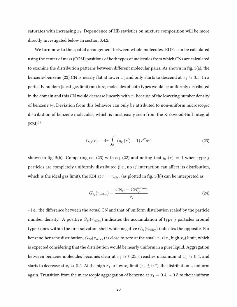
We turn now to the spatial arrangement between whole molecules. RDFs can be calculated

using the center of mass (COM) positions of both types of molecules from which CNs are calculated

to examine the distribution patterns between di�erent molecular pairs. As shown in �g. 5(a), the

benzene-benzene (22) CN is nearly �at at lower x1 and only starts to descend at x1 ≈ 0.5. In a

perfectly random (ideal-gas limit) mixture, molecules of both types would be uniformly distributed

in the domain and this CN would decrease linearly with x1 because of the lowering number density

of benzene ν2. Deviation from this behavior can only be attributed to non-uniform microscopic

distribution of benzene molecules, which is most easily seen from the Kirkwood-Bu� integral

(KBI)75

Gij(r) ≡ 4π

∫ r

0

(gij(r′)− 1) r′2dr′ (23)

shown in �g. 5(b). Comparing eq. (23) with eq. (22) and noting that gij(r) = 1 when type j

particles are completely uniformly distributed (i.e., no ij-interaction can a�ect its distribution,

which is the ideal gas limit), the KBI at r = rvalley (as plotted in �g. 5(b)) can be interpreted as

Gij(rvalley) =CNij − CNuniform

ij

νj(24)

– i.e., the di�erence between the actual CN and that of uniform distribution scaled by the particle

number density. A positive Gij(rvalley) indicates the accumulation of type j particles around

type i ones within the �rst solvation shell while negative Gij(rvalley) indicates the opposite. For

benzene-benzene distribution, G22(rvalley) is close to zero at the small x1 (i.e., high x2) limit, which

is expected considering that the distribution would be nearly uniform in a pure liquid. Aggregation

between benzene molecules becomes clear at x1 ≈ 0.255, reaches maximum at x1 ≈ 0.4, and

starts to decrease at x1 ≈ 0.5. At the high x1 or low x2 limit (x1 & 0.7), the distribution is uniform

again. Transition from the microscopic aggregation of benzene at x1 = 0.4 ∼ 0.5 to their uniform

23

dispersion at higher x1 causes the overall decrease in benzene-benzene interactions. Indeed,

the CN22 pro�le in �g. 5(a) is rather similar to that of Ebind22 pro�le in �g. 3(a) and both have a

downward turn at x1 ≈ 0.51. Analysis of benzene-benzene self-distribution patterns reveals the

second driving mechanism for the changing relative volatility: at high x1, ethanol molecules break

the local benzene aggregates, which exposes individual benzene molecules to the less favorable

benzene-ethanol interactions and thus increases their volatility.

For ethanol-ethanol distribution, G11(rvalley) starts high at the low x1 end and declines steadily

with increasing x1. At x1 & 0.7, ethanol distribution also becomes uniform as it approaches the

pure liquid limit. The trend is consist with the earlier observation from O-H RDFs in �g. 4(a) that

ethanol molecules start to cluster at extremely low x1 but the degree of aggregation, somewhat

unexpectedly, decreases with x1 as the chance for HB binding saturates. This seeming perplexity,

which will be further discussed below in section 3.4.2, becomes comprehensible considering that

the distribution would have to return to near uniformity – i.e., G11(rvalley)→ 1 – at the x1 → 1

limit. Unlike the benzene-benzene case, the CN11 pro�le di�ers considerably from the Ebind11 one:

the latter shows a clear turning point at x1 ≈ 0.2 whereas the former is rather steady in its rise.

Therefore, the transition point inEbind11 and thus the changing volatility of ethanol (the �rst driving

mechanism) cannot be solely accounted for by the changing spatial positions of neighboring

ethanol molecules. The reason is that, compared with the benzene case, interactions between

ethanol molecules are not dominated by the van der Waals (vdW) interaction which is more

isotropic and determined by intermolecular distance. Rather, electrostatic interactions between

the polar OH groups require speci�c relative orientations between ethanol molecules to form HBs.

The importance of HB interactions in explaining the Ebind11 trend is a�rmed by the CNOH pro�le

in �g. 4(b) where a clear turning point is identi�ed at x1 ≈ 0.2, coinciding with that in the Ebind11

pro�le. Direct analysis of HB patterns will be performed in section 3.4.2.

Finally, for cross-species intermolecular arrangement, G12(rvalley) (which equals G21(rvalley))

stays closer to zero for the entire composition range, indicating a weaker e�ect of cross-species

interactions on molecular arrangement. Both CN12 and CN21 vary nearly linearly with compo-

24

0.0 0.2 0.4 0.6 0.8 1.0x1

0

3

6

9

12

Norm

alize

d N

HB

2NHB/N12NHB/N1/x1

Figure 6: Composition-dependence (in the liquid phase at VLE) of the average number of HBconnections per ethanol molecule 2NHB/N1 and the same number scaled by ethanol mole fraction

2NHB/(x1N1). (Error bars smaller than the marker size are not shown.)

sition, roughly in proportion to the corresponding number densities, ν2 and ν1. Both pro�les

show a small dip – a range of negative deviation – at 0.2 . x1 . 0.5, as a result of microscopic

aggregation within the same species.

3.4.2 Hydrogen Bonding Analysis

Observations made so far point toward a three-stage process behind the apparent steady

decline of (GE1 − GE

2)/RT (�g. 2). The �rst transition, between stages 1 and 2, occurs at x1 ≈ 0.2

and is marked by the plateauing of Ebind1 . The second transition, between stages 2 and 3, occurs at

x1 ≈ 0.5, i.e., shortly after the azeotrope, and is responsible for the later drop ofEbind2 . The previous

section (section 3.4.1) showed that the second transition can be explained by the dismantlement

of benzene-benzene microscopic aggregation, which exposes benzene molecules to less favorable

cross-species interactions with ethanol. However, the �rst transition is less clear from the spatial

arrangement of ethanol molecules, as far as their RDF and KBI show. It was suggested that

ethanol-ethanol interaction is dominated by HB interactions which are not determined by the

COM positions of ethanol molecules alone. This section thus focuses on the direct analysis of HB

formation patterns between ethanol molecules.

With the electron donor O and acceptor H atoms in the hydroxyl group, ethanol molecules can

easily form HBs through which the possibility of forming molecular clusters or even networks is

25

foreseeable. In this study, HBs are de�ned according to the classical geometric criterion76–78 – a

HB pair is identi�ed when all of the following three conditions are met:

1. the distance between the O atoms on the two interacting −OH groups is ≤ 3.5 Å;

2. the distance between the donor O and acceptor H atoms is ≤ 2.6 Å; and

3. the H−O···O angle is ≤ 30°.

Following this standard, the total number of HBs in the liquid cell NHB can be found and the

average number of HB connections seen by each ethanol molecule is 2NHB/N1 (the factor of 2 is

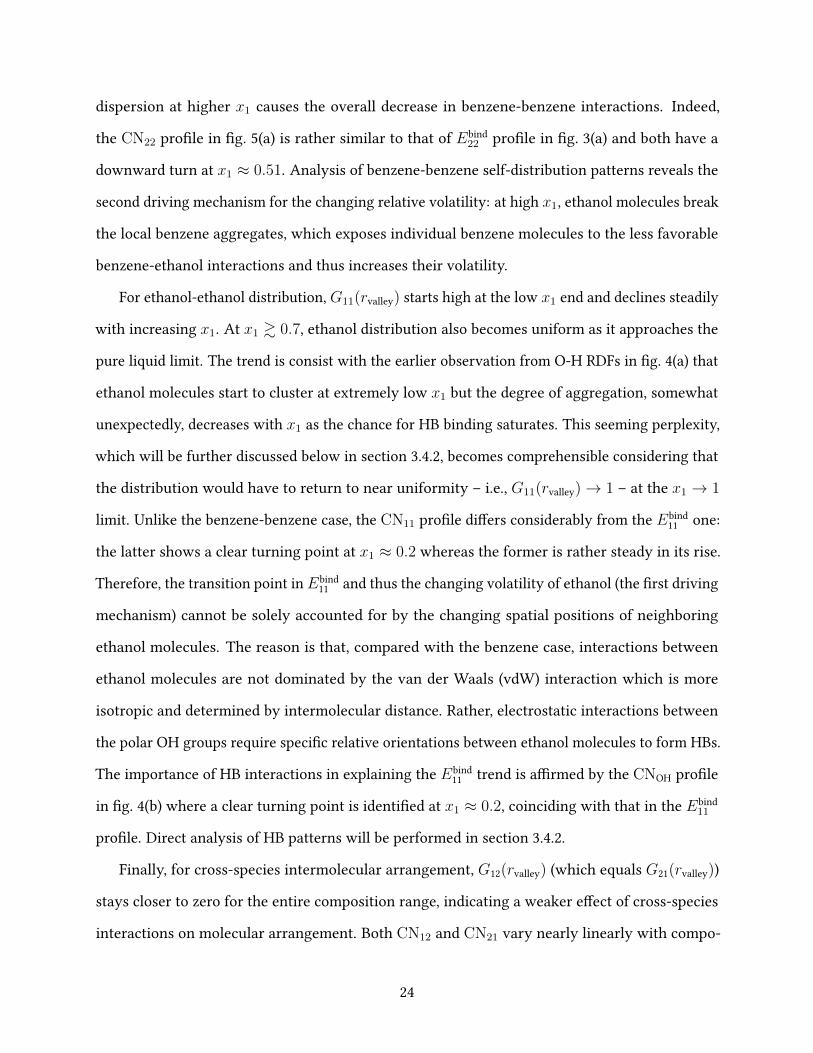
because each HB connects 2 ethanol molecules). As shown in �g. 6, ethanol starts to form HBs at

very low concentration. (At the lowest ethanol concentration simulated, i.e., x1 = 0.008, there

are on average less than 3 ethanol molecules in the simulation cell and HBs are rare. That case

is not shown in �g. 6 owing to the lack of statistics. The leftmost point in �g. 6 is x1 = 0.086

where 2NHB/N1 already exceeds 1.) Although the number of HBs connected to each molecule

does initially increase with concentration, the increase rate tapers o� very quickly: at x1 = 0.181,

2NHB/N1 reaches 1.359, which is not much lower than that of the highest concentration in �g. 6:

2NHB/N1 = 1.653 at x1 = 0.966. For comparison, Saiz et al. 79 calculated the HB statistics of

pure ethanol from molecular dynamics results and at a very close temperature of T = 348 K,

their 2NHB/N1 = 1.72. Using a slightly di�erent set of HB identi�cation criteria and for a lower

T = 300 K, Noskov et al. 80 reported the number to be 1.65 again for pure ethanol. Therefore, on

average, each ethanol molecule has fewer than 2 HB connections and, from our results, it becomes

clear that ethanol gets close to this �nal limit very early on – starting from x1 ≈ 0.2.

Since HB is a binary interaction, if we neglect the saturation of HB and resort to a simplistic

mean-�eld argument, the chance for any one molecule to form HBs would be proportional to

the concentration of other ethanol molecules in its surroundings – i.e., proportional to x1. A

scaled measure of the extent of HB formation is thus 2NHB/(x1N1) which is also plotted in �g. 6.

This number drops monotonically with increasing x1 because of the early saturation of 2NHB/N1:

for an average ethanol molecule, once its number of HB connections gets close to (but lower

than) 2, connecting with additional ethanol molecules in its surroundings becomes drastically

26

0.0 0.2 0.4 0.6 0.8 1.0x1

0

4

8

12

16

20

Aver

age

clust

er si

ze0

1

2

3

4

Poly

disp

ersit

y in

dexNn

Nw

Nw/Nn

Figure 7: Composition-dependence (in the liquid phase at VLE) of (left/blue) the number average(Nn) and weight average (Nw) size of ethanol HB clusters and (right/red) their polydispersity

index (PDI) Nw/Nn. (Error bars smaller than the marker size are not shown.)

more di�cult, even though there are many more of them around as x1 increases. The decline

of G11(rvalley) with increasing x1, as observed in �g. 5(b), can be similarly explained. In eq. (24),

CNuniform11 strictly conforms to the mean-�eld argument and increases in proportion to x1. For

actual CN11, surrounding ethanol molecules found around a reference ethanol molecule can be

divided into two groups: (1) those forming HBs with the reference molecule and (2) additional

molecules not HB-connected with the reference but happened to appear nearby. The number in

group (2) is approximately proportional to x1 (and thus to CNuniform11 ), whereas that of group (1)

saturates to a nearly constant level at very low x1. The KBI, as the di�erence between CN11 and

CNuniform11 scaled by ν1 (which is proportional to x1), must thus decrease with x1.

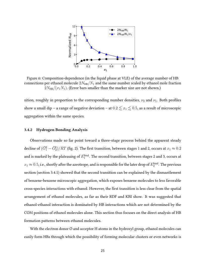
Clusters formed by ethanol molecules interconnected through HBs can be identi�ed by assign-

ing any two molecules sharing at least one HB to the same cluster. The number-average (Nn) and

weight-average (Nw) cluster sizes are plotted against x1 in �g. 7. Both measures of cluster size

initially increase with ethanol concentration but after x1 ≈ 0.2 the trend signi�cantly slows down.

This transition is clearly associated with the near saturation of HB connections of each molecule,

which also coincides with the slowdown of the rising ethanol-ethanol interaction contribution to

binding energy Ebind11 at the same x1 level (�g. 3(a)). Direct correspondence between HB statistics

and Ebind11 is predictable as HB interactions are expected to dominate the ethanol-ethanol interac-

tions. What is interesting is a clear separation of trends between Nn and Nw occurring around

27

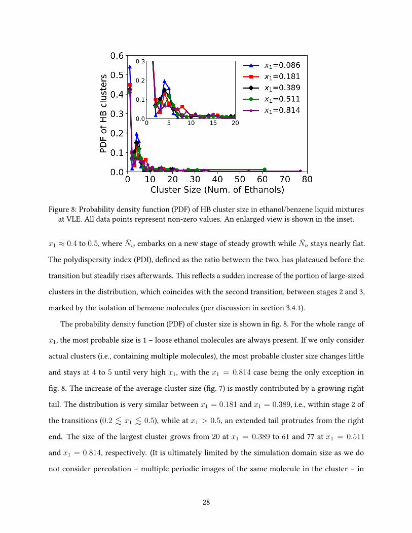
Figure 8: Probability density function (PDF) of HB cluster size in ethanol/benzene liquid mixturesat VLE. All data points represent non-zero values. An enlarged view is shown in the inset.

x1 ≈ 0.4 to 0.5, where Nw embarks on a new stage of steady growth while Nn stays nearly �at.

The polydispersity index (PDI), de�ned as the ratio between the two, has plateaued before the

transition but steadily rises afterwards. This re�ects a sudden increase of the portion of large-sized

clusters in the distribution, which coincides with the second transition, between stages 2 and 3,

marked by the isolation of benzene molecules (per discussion in section 3.4.1).

The probability density function (PDF) of cluster size is shown in �g. 8. For the whole range of

x1, the most probable size is 1 – loose ethanol molecules are always present. If we only consider

actual clusters (i.e., containing multiple molecules), the most probable cluster size changes little

and stays at 4 to 5 until very high x1, with the x1 = 0.814 case being the only exception in

�g. 8. The increase of the average cluster size (�g. 7) is mostly contributed by a growing right

tail. The distribution is very similar between x1 = 0.181 and x1 = 0.389, i.e., within stage 2 of

the transitions (0.2 . x1 . 0.5), while at x1 > 0.5, an extended tail protrudes from the right

end. The size of the largest cluster grows from 20 at x1 = 0.389 to 61 and 77 at x1 = 0.511

and x1 = 0.814, respectively. (It is ultimately limited by the simulation domain size as we do

not consider percolation – multiple periodic images of the same molecule in the cluster – in

28

our cluster size measurement.) These “super” clusters likely result from the merger of smaller

ones. Between x1 ≈ 0.2 and x1 ≈ 0.5, most clusters are formed by a few ethanol molecules and

increasing x1 must lead to a higher number density of such primary clusters. Shortening distance

between clusters facilitates their coalition. For a molecule to bridge two primary clusters, it only

needs to have two HB connections, one with each primary cluster, which compared with the

domain average 2NHB/N1 value is only slightly higher. Formation of a small number of super

clusters through coalition can thus quickly bring up the weight-average cluster size Nw (�g. 7)

without substantially a�ecting the average HB number (�g. 6), which is totally consistent with

our observations.

Our �nding here, that HB clusters continue to grow with x1 beyond the azeotropic composition,

contradicts the claim by Shephard et al. 34 that in the methanol-benzene system they studied using

the EPSR modeling approach, methanol molecules form larger clusters at the azeotrope than in its

pure state. In their results, methanol clusters with up to 20 molecules were found at the azeotrope,

which is comparable to our x1 = 0.389 case, but in pure methanol, the cluster size rarely exceeds

10. Other studies, however, have routinely reported large clusters containing O(100) or more

molecules in pure ethanol (and other small aliphatic alcohols as well), which varies with the

system size, modeling method, and identi�cation criteria81,82. In our highest x1 = 0.966 case,

the largest cluster contains 81 ethanol molecules, which is comparable to most previous studies

despite our smaller system size and higher temperature.

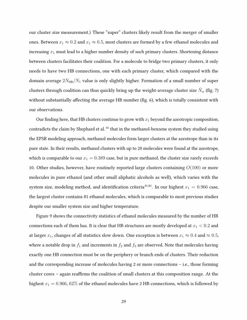
Figure 9 shows the connectivity statistics of ethanol molecules measured by the number of HB

connections each of them has. It is clear that HB structures are mostly developed at x1 < 0.2 and

at larger x1, changes of all statistics slow down. One exception is between x1 ≈ 0.4 and ≈ 0.5,

where a notable drop in f1 and increments in f2 and f3 are observed. Note that molecules having

exactly one HB connection must be on the periphery or branch ends of clusters. Their reduction

and the corresponding increase of molecules having 2 or more connections – i.e., those forming

cluster cores – again rea�rms the coalition of small clusters at this composition range. At the

highest x1 = 0.966, 62% of the ethanol molecules have 2 HB connections, which is followed by

29

0.0 0.2 0.4 0.6 0.8 1.0x1

0.0

0.2

0.4

0.6

0.8

1.0

Etha

nol F

ract

ion

f0f1

f2f3

Figure 9: HB connectivity statistics of ethanol molecules in liquid mixtures with benzene at VLE:fn is the fraction of ethanol molecules having n HB connections. (The �rst point is at x1 = 0.008;

error bars are smaller than the marker size and thus not shown.)

26% having 1 HB connection. This indicates that most HB clusters are chain-like structures where

the middle members all have two connections and the end ones have one. Indeed, at least for

pure methanol and ethanol, it has been well established in the literature that molecular chains

are the predominant cluster form34,76,77,79. Only a very small portion (5.1%) of ethanol molecules

have 3 connections which can serve as branching points in a cluster. The remaining 6.9% are

loose molecules not attached to any cluster. This distribution is very much consistent with earlier

analysis79 of pure ethanol at T = 348 K where (f0, f1, f2, f3) = (0.042, 0.245, 0.664, 0.049).

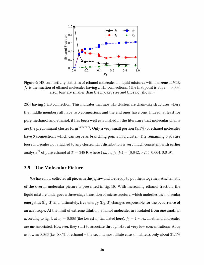
3.5 The Molecular Picture

We have now collected all pieces in the jigsaw and are ready to put them together. A schematic

of the overall molecular picture is presented in �g. 10. With increasing ethanol fraction, the

liquid mixture undergoes a three-stage transition of microstructure, which underlies the molecular

energetics (�g. 3) and, ultimately, free energy (�g. 2) changes responsible for the occurrence of

an azeotrope. At the limit of extreme dilution, ethanol molecules are isolated from one another:

according to �g. 9, at x1 = 0.008 (the lowest x1 simulated here), f0 = 1 – i.e., all ethanol molecules

are un-associated. However, they start to associate through HBs at very low concentrations. At x1

as low as 0.086 (i.e., 8.6% of ethanol – the second most dilute case simulated), only about 31.1%

30

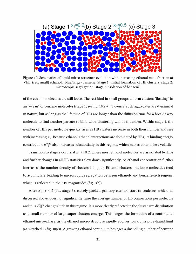
(a) Stage 1 (b) Stage 2 (c) Stage 3x1≈0.2 x1≈0.5

Figure 10: Schematics of liquid mirco-structure evolution with increasing ethanol mole fraction atVEL: (red/small) ethanol; (blue/large) benzene. Stage 1: initial formation of HB clusters; stage 2:

microscopic segregation; stage 3: isolation of benzene.

of the ethanol molecules are still loose. The rest bind in small groups to form clusters “�oating” in

an “ocean” of benzene molecules (stage 1; see �g. 10(a)). Of course, such aggregates are dynamical

in nature, but as long as the life time of HBs are longer than the di�usion time for a break-away

molecule to �nd another partner to bind with, clustering will be the norm. Within stage 1, the

number of HBs per molecule quickly rises as HB clusters increase in both their number and size

with increasing x1. Because ethanol-ethanol interactions are dominated by HBs, its binding energy

contribution Ebind11 also increases substantially in this regime, which makes ethanol less volatile.

Transition to stage 2 occurs at x1 ≈ 0.2, where most ethanol molecules are associated by HBs

and further changes in all HB statistics slow down signi�cantly. As ethanol concentration further

increases, the number density of clusters is higher. Ethanol clusters and loose molecules tend

to accumulate, leading to microscopic segregation between ethanol- and benzene-rich regions,

which is re�ected in the KBI magnitudes (�g. 5(b)).

After x1 ≈ 0.5 (i.e., stage 3), closely-packed primary clusters start to coalesce, which, as

discussed above, does not signi�cantly raise the average number of HB connections per molecule

and thusEbind11 changes little in this regime. It is more clearly re�ected in the cluster size distribution

as a small number of large super clusters emerge. This forges the formation of a continuous

ethanol micro-phase, as the ethanol micro-structure rapidly evolves toward its pure-liquid limit

(as sketched in �g. 10(c)). A growing ethanol continuum besieges a dwindling number of benzene

31

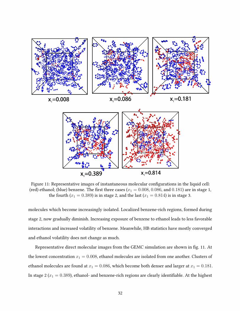
Figure 11: Representative images of instantaneous molecular con�gurations in the liquid cell:(red) ethanol; (blue) benzene. The �rst three cases (x1 = 0.008, 0.086, and 0.181) are in stage 1,

the fourth (x1 = 0.389) is in stage 2, and the last (x1 = 0.814) is in stage 3.

molecules which become increasingly isolated. Localized benzene-rich regions, formed during

stage 2, now gradually diminish. Increasing exposure of benzene to ethanol leads to less favorable

interactions and increased volatility of benzene. Meanwhile, HB statistics have mostly converged

and ethanol volatility does not change as much.

Representative direct molecular images from the GEMC simulation are shown in �g. 11. At

the lowest concentration x1 = 0.008, ethanol molecules are isolated from one another. Clusters of

ethanol molecules are found at x1 = 0.086, which become both denser and larger at x1 = 0.181.

In stage 2 (x1 = 0.389), ethanol- and benzene-rich regions are clearly identi�able. At the highest

32

concentration shown (x1 = 0.814), benzene molecules are nearly all isolated and surrounded by

an ethanol continuum.

We expect this molecular mechanism to be generalizable to similar positive azeotropes

where one component is signi�cantly more polar than the other and has a strong tendency

to self-associate, such as methanol/benzene or even chloroform/methanol. However, for positive

azeotropes where both components are polar and strong association can occur within both species

as well as between species, such as ethanol/water, patterns of molecular arrangement at di�erent

composition levels are expected to be di�erent. On the other hand, for negative azeotropes, such

as water/formic acid or acetone/chloroform, cross-species association in the mixture might be

stronger than that between molecules of the same species and thus a di�erent mechanism is

also expected. Our most signi�cant contribution is the demonstration of a new approach for

azeotrope study, which focuses on thermodynamic properties and liquid microstructure variations

over a wider composition range than the azeotrope point. Speci�c molecular mechanisms arising

from this approach would di�er between di�erent types of azeotropes. Its application to broader

systems is still needed. Finally, we note that the thermodynamic criterion discussed in section 3.2

is generally applicable to all azeotrope systems, except that for negative azeotropes, the two

inequalities in eq. (13) must be swapped between the x1 < xaze1 and x1 > xaze

1 cases.

4 Conclusions

In this study, GEMC is used to investigate the VLE behavior of the ethanol/benzene mixture

over the entire composition range. The simulation results reproduce the experimental phase

diagram, including an accurate prediction of the azeotrope point. We emphasize that the necessary

and su�cient condition for the occurrence of azeotrope is the changing order of relative volatility

between the two components. For the ethanol/benzene system studied here, which has a positive

azeotrope, ethanol is more volatile than benzene at x1 < xaze1 whereas benzene becomes more

volatile at x1 > xaze1 . Molecular understanding of azeotrope formation thus requires the explanation

33

of the changing volatility of the two components over a much wider composition range than the

azeotrope point itself.

A thermodynamic criterion has thus been derived based on the comparison of partial excess

Gibbs energy between the two components (eqs. (11) and (13)). Application to the ethanol/benzene

system simulated in this study shows that there are at least two stages of di�erent dominant

mechanisms for the changing relative volatility. At lower ethanol mole fraction x1, volatility of

ethanol decreases signi�cantly with increasing x1 while that of benzene stays nearly constant.

At higher x1, ethanol volatility no longer changes but benzene becomes increasingly volatile.

Analysis of molecular energetics shows that these free energy variations are dominated by energetic

interactions, especially self-interactions between molecules of the same species. As x1 increases,

at lower x1, each ethanol molecule feels stronger total attraction from other ethanol molecules in

the mixture, whereas at higher x1, each benzene molecule feels less total attraction from other

benzene molecules.

Molecular energetics is studied through the microscopic liquid structure, using RDF, KBI, and

HB analysis. It is concluded that with increasing x1, there are three stages of di�erent molecular

organization patterns. HBs start to form at very low x1 and in stage 1, ethanol molecules quickly

cluster in the ocean of benzene. Cluster size and density increase with increasing x1. In stage 2,

which for the conditions studied here starts at x1 ≈ 0.2, ethanol clusters further aggregate and

cause microscopic segregation between ethanol- and benzene-rich regions. In stage 3, which

starts at x1 ≈ 0.5, further increasing x1 results in the coalition of smaller clusters into larger ones

and ethanol forms a continuous phase, leaving benzene molecules increasingly isolated. Since

stage 1 sees most increase in the number of HBs per molecule, it is where ethanol molecules are

increasingly attracted in the liquid phase and become less volatile. At higher x1, HB increments

are much slower, which explains the later plateauing of ethanol volatility. Meanwhile, throughout

stages 1 and 2, benzene molecules are surrounded mostly by other benzene molecules. This only

changes in stage 3, where ethanol clusters are large and dense enough to cause the ghettoization

of benzene and its increasing isolation. Higher exposure to ethanol causes its raised volatility in

34

this regime.

This is to our knowledge the �rst full molecular mechanism for the existence of azeotrope

considering the variations in thermodynamic properties over the whole composition range. It

is expected to be generalizable to other systems with positive azeotropes between a polar and

non-polar species.

Acknowledgment

The authors acknowledge the �nancial support by the Natural Sciences and Engineering

Research Council (NSERC) of Canada (RGPIN-4903-2014) and the National Natural Science Foun-

dation of China (NFSC; No. 21878219). We also acknowledge Compute/Calcul Canada for its

allocation of computing resource. DL would like to thank the China Scholarship Council (CSC)

for supporting his doctoral study at McMaster University (No. 201500090106). This work is also

made possible by the facilities of the Shared Hierarchical Academic Research Computing Network

(SHARCNET: www.sharcnet.ca).

A Cohesive energy and binding energy

In this appendix, we give detailed mathematical de�nitions of cohesive and binding energies

and discuss the conceptual relationships between energetic quantities.

A.1 Cohesive energy

In a binary mixture, the molar cohesive energy Ecoh is calculated according to its de�nition

Ecoh≡x1Eiso1 + x2E

iso2 − Ebulk (25)

35

where Ebulk is the molar potential energy of the liquid mixture and

Eiso1 = NAV〈eiso1 〉 (26)

Eiso2 = NAV〈eiso2 〉 (27)

are the potential energy of in�nitely-separated molecules of component 1 and 2, respectively

(scaled to the basis of 1 mol of the species), when each molecule is isolated in a vacuum83. In

eq. (26) and eq. (27), eiso1 and eiso2 are the energy of one single molecule placed in a vacuum, NAv

is the Avogadro constant, and 〈·〉 indicates ensemble average. The potential energy Ebulk is

the summation of bonded (bond stretching, bending, and torsion potentials – see table 2) and

non-bonded or pairwise (Lennard-Jones and Coulombic potentials) interactions and the latter is

further divided into intra- and intermolecular components:

Ebulk = Ebonded + Enon-bonded = Ebonded + E intra + E inter (28)

where all these terms are on the basis of 1 mole of the mixture. Between the bulk liquid and

isolated state, the energy contained within each molecule changes very little: i.e.

Ebonded + E intra ≈ x1Eiso1 + x2E

iso2 (29)

which, combined with eqs. (25) and (28), leads to eq. (18). The cohesive energy is thus directly

related to the total intermolecular pairwise interactions in the mixture. The latter is the summation

of the interactions between all individual molecular pairs

E inter =1

2

n1∑ι=1

n1∑κ=1κ6=ι

e11(ι, κ) +1

2

n2∑ι=1

n2∑κ=1κ6=ι

e22(ι, κ) +

n1∑ι=1

n2∑κ=1

e12(ι, κ) (30)

where ι and κ are indices for molecules, ni is the number of molecules of type i in 1 mol of the

mixture, and eij(ι, κ) is the interaction potential between molecule ι of type i and molecule κ of

36

type j. The �rst two terms are interactions between molecules of the same type and a factor of

1/2 is needed because each pair is counted twice in the double-loop summation.

A.2 Binding energy

To strip one component-1 molecule, indexed by ι, away from the mixture to in�nite distance,

its pairwise intermolecular interactions with all other molecules, which remain in place, must be

broken. The energy required is

ebind1 (ι) = ebind

11 + ebind12 ≈ −

n1∑κ=1κ6=ι

e11(ι, κ) +

n2∑κ=1

e12(ι, κ)

(31)

(the approximate sign ≈ again would become an equal sign = if we assume no change in the

bonded and intramolecular non-bonded interactions as the molecule leaves the liquid phase). The

two summations on the right-hand side correspond to contributions from self-interaction (with

other molecules of component 1) ebind11 and cross-interaction (with molecules of component 2) ebind

12 ,

respectively. Scaling this energy, which is for the removal of a single molecule, to the per mole (of

component 1) basis, we obtain the molar binding energy of component 1

Ebind1 = Ebind

11 + Ebind12 ≈ −

1

x1

n1∑ι=1

n1∑κ=1κ6=ι

e11(ι, κ) +

n2∑κ=1

e12(ι, κ)

(32)

which is again decomposed into self- and cross-interaction terms Ebind11 and Ebind

12 . The molar

binding energy of component 2

Ebind2 = Ebind

22 + Ebind21 ≈ −

1

x2

n2∑κ=1

n2∑ι=1ι6=κ

e22(ι, κ) +

n1∑ι=1

e12(ι, κ)

(33)

is likewise de�ned.

37

Calculation Ebind1 is calculated by �rst carving out all component-2 molecules from the sim-

ulation cell while leaving component-1 molecules frozen in place. The cohesive energy of the

resulting cell contains contributions from 1-1 self interactions only, from which Ebind11 can be

calculated. Likewise, Ebind22 is calculated by removing all component-1 molecules in the cell. The

cross-terms, i.e., Ebind12 or Ebind

21 , can then be calculated from the cohesive energy of the original

mixture cell as well as the above results by invoking eqs. (18) and (30).

Comparison with partial molar energy It is natural to draw connection between molar

binding energy and partial molar energy, both of which appear to describe marginal energy

changes associated with adding or removing molecules. These two quantities are conceptually

related but not the same. Discussion here thus attempts to make a distinction between them.

Partial molecular energy measures the marginal changes in energy caused by the addition of a

di�erentially small amount of one component, also scaled to the basis of 1 mol of the species

concerned. In our de�nition, −Ebind1 (or −Ebind

2 ; minus sign because binding energy is de�ned

based on the removal rather than addition of the molecules) clearly has a similar physical meaning,

but it misses two important components in partial molar energy: (1) the intramolecular energy

components (bonded and non-bonded) and (2), more importantly, energy changes caused by the

reorganization of the remaining molecules after the addition or removal of the selected molecule. It

is, however, much more straightforward to compute, which only requires the system con�guration.

In comparison, computation of partial properties typically requires either particle insertion with

ensemble sampling or numerical di�erentiation over di�erent composition levels, which remains

a non-trivial challenge especially for polyatomic molecular �uids84,85.

Relationship with cohesive energy Combining eqs. (18), (30), (32) and (33), we now get

E inter ≈ −Ecoh = −1

2

(x1E

bind1 + x2E

bind2

)(34)

38

(the second relation is = because the errors due to the slightly di�erent bonded and intramolecular

non-bonded interactions between the isolated and condensed states of individual molecules are

contained in both eq. (18) and eqs. (32) and (33), allowing them to cancel one another). Equation (34)

is reminiscent of the summability relation between the mixture molar energy and component

partial molar energies

U = x1U1 + x2U2 (35)

and, therefore, −(1/2)Ebind1 and −(1/2)Ebind

2 can be similarly interpreted as the contributions to

the liquid-phase intermolecular interactions E inter from individual components. The factor of 1/2

in eq. (34) is because the intermolecular interaction between each pair of molecules is counted

twice in Ebind1 and Ebind

2 combined.

References

(1) Jürgen Gmehling, Ulfert Onken, Dieter Behrens, and R Eckermann. Vapor-liquid equilibrium

data collection: Aqueous-organic systems, volume 1. Dechema Frankfurt, Germany, 1977. Part

1.

(2) Jürgen Gmehling, J Menke, J Krafczyk, K Fischer, S Pereira Nunes, and K Peinemann.

Azeotropic data. Wiley Online Library, 1994.

(3) Jürgen Gmehling and Christian Möllmann. Synthesis of distillation processes using thermo-

dynamic models and the dortmund data bank. Industrial & engineering chemistry research, 37

(8):3112–3123, 1998.

(4) Michael L Michelsen. A method for incorporating excess gibbs energy models in equations

of state. Fluid Phase Equilibria, 60(1-2):47–58, 1990.

39

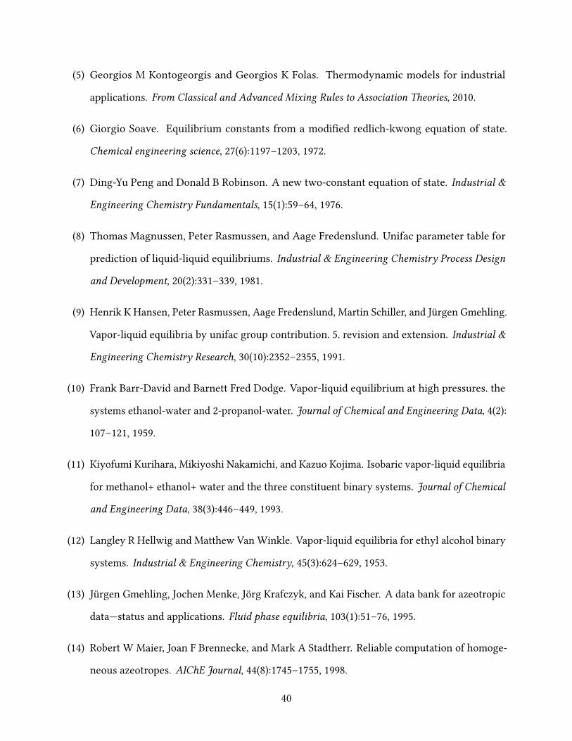
(5) Georgios M Kontogeorgis and Georgios K Folas. Thermodynamic models for industrial

applications. From Classical and Advanced Mixing Rules to Association Theories, 2010.

(6) Giorgio Soave. Equilibrium constants from a modi�ed redlich-kwong equation of state.

Chemical engineering science, 27(6):1197–1203, 1972.

(7) Ding-Yu Peng and Donald B Robinson. A new two-constant equation of state. Industrial &

Engineering Chemistry Fundamentals, 15(1):59–64, 1976.

(8) Thomas Magnussen, Peter Rasmussen, and Aage Fredenslund. Unifac parameter table for

prediction of liquid-liquid equilibriums. Industrial & Engineering Chemistry Process Design

and Development, 20(2):331–339, 1981.

(9) Henrik K Hansen, Peter Rasmussen, Aage Fredenslund, Martin Schiller, and Jürgen Gmehling.

Vapor-liquid equilibria by unifac group contribution. 5. revision and extension. Industrial &

Engineering Chemistry Research, 30(10):2352–2355, 1991.

(10) Frank Barr-David and Barnett Fred Dodge. Vapor-liquid equilibrium at high pressures. the

systems ethanol-water and 2-propanol-water. Journal of Chemical and Engineering Data, 4(2):

107–121, 1959.

(11) Kiyofumi Kurihara, Mikiyoshi Nakamichi, and Kazuo Kojima. Isobaric vapor-liquid equilibria

for methanol+ ethanol+ water and the three constituent binary systems. Journal of Chemical

and Engineering Data, 38(3):446–449, 1993.

(12) Langley R Hellwig and Matthew Van Winkle. Vapor-liquid equilibria for ethyl alcohol binary

systems. Industrial & Engineering Chemistry, 45(3):624–629, 1953.

(13) Jürgen Gmehling, Jochen Menke, Jörg Krafczyk, and Kai Fischer. A data bank for azeotropic

data—status and applications. Fluid phase equilibria, 103(1):51–76, 1995.

(14) Robert W Maier, Joan F Brennecke, and Mark A Stadtherr. Reliable computation of homoge-

neous azeotropes. AIChE Journal, 44(8):1745–1755, 1998.

40

(15) Noelia Calvar, Begoña González, Elena Gómez, and A Domínguez. Study of the behaviour

of the azeotropic mixture ethanol–water with imidazolium-based ionic liquids. Fluid Phase

Equilibria, 259(1):51–56, 2007.

(16) G Onori. Structural properties of aqueous mixtures of monohydric alcohols from near-infrared

absorption spectra. Chemical physics letters, 154(3):213–216, 1989.

(17) Robert W Williams, James L Cheh, Alfred H Lowrey, and Alan F Weir. E�ects of hydration

on scale factors for ab initio force constants. 9. methanol. The Journal of Physical Chemistry,

99(15):5299–5307, 1995.

(18) Akihiro Wakisaka, Hassan Abdoul-Carime, Yoshitaka Yamamoto, and Yoshimichi Kiyozumi.

Non-ideality of binary mixtures water-methanol and water-acetonitrile from the viewpoint

of clustering structure. Journal of the Chemical Society, Faraday Transactions, 94(3):369–374,

1998.

(19) Pedro D Vaz, Mariela M Nolasco, Francisco PSC Gil, Paulo JA Ribeiro-Claro, and John

Tomkinson. Hydrogen-bond dynamics of c-h-o interactions: The chloroform–acetone case.

Chemistry–A European Journal, 16(30):9010–9017, 2010.

(20) Charles M Huggins, George C Pimentel, and James N Shoolery. Proton magnetic resonance

studies of chloroform in solution: evidence for hydrogen bonding. The Journal of Chemical

Physics, 23(7):1244–1247, 1955.

(21) K Choi and DW Tedder. Molecular interactions in chloroform-diluent mixtures. AIChE

journal, 43(1):196–211, 1997.

(22) Masaki Matsumoto, Nobuyuki Nishi, Toshiya Furusawa, Masaru Saita, Toshiyuki Takamuku,

Motoyuki Yamagami, and Toshio Yamaguchi. Structure of clusters in ethanol–water binary

solutions studied by mass spectrometry and x-ray di�raction. Bulletin of the Chemical Society

of Japan, 68(7):1775–1783, 1995.

41

(23) MR Jalilian and L Alibabaei. Spectra and structure of binary azeotropes: I. acetone–chloroform.

Spectrochimica Acta Part A: Molecular and Biomolecular Spectroscopy, 62(1-3):322–325, 2005.

(24) TS Perova, Daniel H Christensen, and O Faurskov Nielsen. Low-frequency raman and

far-infrared spectra of acetone/chloroform mixtures. Vibrational spectroscopy, 15(1):61–67,

1997.

(25) MR Jalilian. Spectra and structure of binary azeotropes: Ii. acetone–n-pentane. Spectrochimica

Acta Part A: Molecular and Biomolecular Spectroscopy, 66(1):91–93, 2007.

(26) MR Jalilian and Sayyed Faramarz Tayyari. Spectra and structure of binary azeotropes vi-

benzene-methanol. Spectrochimica Acta Part A: Molecular and Biomolecular Spectroscopy, 73

(5):828–832, 2009.

(27) MR Jalilian. Spectra and structure of binary azeotropes: Iv. acetone–cyclohexane. Spec-

trochimica Acta Part A: Molecular and Biomolecular Spectroscopy, 69(3):812–815, 2008.

(28) MR Jalilian and Mansoureh Zahedi-Tabrizi. Spectra and structure of binary azeotropes v-

acetone–cyclopentane. Spectrochimica Acta Part A: Molecular and Biomolecular Spectroscopy,

69(1):278–281, 2008.

(29) Juan D Ripoll, Sol M Mejía, Matthew JL Mills, and Aída L Villa. Understanding the azeotropic

diethyl carbonate–water mixture by structural and energetic characterization of dec(h2o)n

heteroclusters. Journal of molecular modeling, 21(4):93, 2015.

(30) Gergely Matisz, Anne-Marie Kelterer, Walter MF Fabian, and Sándor Kunsági-Máté. Coor-

dination of methanol clusters to benzene: a computational study. The Journal of Physical

Chemistry A, 115(38):10556–10564, 2011.

(31) Budi Waluyo, ING Wardana, Lilis Yuliati, and Mega Nur Sasongko. The role of molecule

cluster on the azeotrope and boiling points of isooctane-ethanol blend. Fuel, 215:178–186,

2018.

42

(32) Barath Baburao, Donald P Visco, and Titus V Albu. Association patterns in (hf)m (h2o)n (m +

n= 2-8) clusters. The Journal of Physical Chemistry A, 111(32):7940–7956, 2007.

(33) Sol M Mejía, Juan F Espinal, and Fanor Mondragón. Cooperative e�ects on the structure and

stability of (ethanol)3–water,(methanol)3–water heterotetramers and (ethanol)4, (methanol)4

tetramers. Journal of Molecular Structure: THEOCHEM, 901(1-3):186–193, 2009.

(34) JJ Shephard, SK Callear, S Imberti, JSO Evans, and CG Salzmann. Microstructures of negative

and positive azeotropes. Physical Chemistry Chemical Physics, 18(28):19227–19235, 2016.

(35) AK Soper. Empirical potential monte carlo simulation of �uid structure. Chemical Physics,

202(2-3):295–306, 1996.

(36) AK Soper. Partial structure factors from disordered materials di�raction data: An approach

using empirical potential structure re�nement. Physical Review B, 72(10):104204, 2005.

(37) Akihiro Wakisaka and Kazuo Matsuura. Microheterogeneity of ethanol–water binary mix-

tures observed at the cluster level. Journal of molecular liquids, 129(1-2):25–32, 2006.

(38) Akihiro Wakisaka, Kazuo Matsuura, Makoto Uranaga, Taisuke Sekimoto, and Mamoru Taka-

hashi. Azeotropy of alcohol–water mixtures from the viewpoint of cluster-level structures.

Journal of Molecular Liquids, 160(2):103–108, 2011.

(39) Akihiro Wakisaka and Toru Iwakami. Molecular clustering inherent in the liquid state: E�ect

of relativity in intermolecular interaction energy. Journal of Molecular Liquids, 189:44–51,

2014.

(40) Athanassios Z Panagiotopoulos. Direct determination of phase coexistence properties of

�uids by monte carlo simulation in a new ensemble. Molecular Physics, 61(4):813–826, 1987.

(41) Athanassios Z Panagiotopoulos, N Quirke, M Stapleton, and DJ Tildesley. Phase equilibria by

simulation in the gibbs ensemble: alternative derivation, generalization and application to

mixture and membrane equilibria. Molecular Physics, 63(4):527–545, 1988.

43

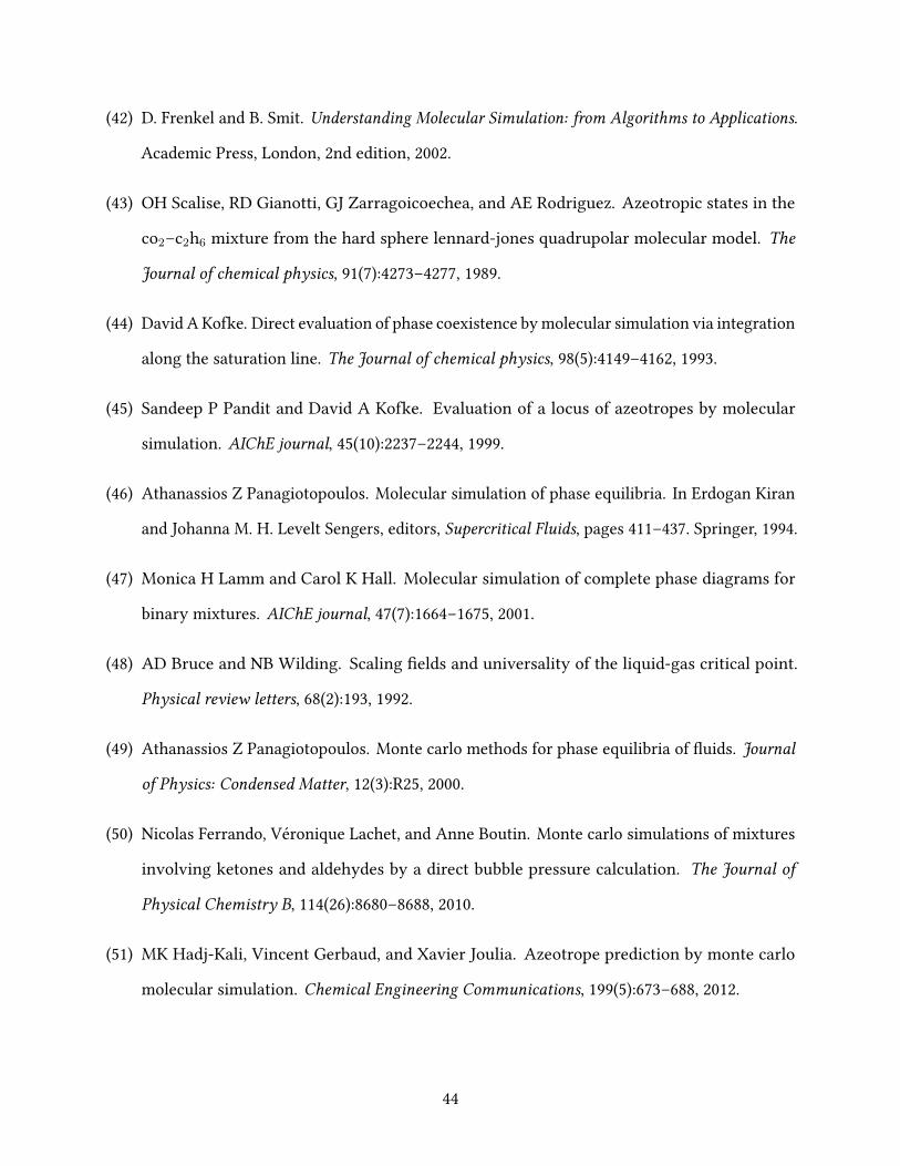
(42) D. Frenkel and B. Smit. Understanding Molecular Simulation: from Algorithms to Applications.

Academic Press, London, 2nd edition, 2002.

(43) OH Scalise, RD Gianotti, GJ Zarragoicoechea, and AE Rodriguez. Azeotropic states in the

co2–c2h6 mixture from the hard sphere lennard-jones quadrupolar molecular model. The

Journal of chemical physics, 91(7):4273–4277, 1989.

(44) David A Kofke. Direct evaluation of phase coexistence by molecular simulation via integration

along the saturation line. The Journal of chemical physics, 98(5):4149–4162, 1993.

(45) Sandeep P Pandit and David A Kofke. Evaluation of a locus of azeotropes by molecular

simulation. AIChE journal, 45(10):2237–2244, 1999.

(46) Athanassios Z Panagiotopoulos. Molecular simulation of phase equilibria. In Erdogan Kiran

and Johanna M. H. Levelt Sengers, editors, Supercritical Fluids, pages 411–437. Springer, 1994.

(47) Monica H Lamm and Carol K Hall. Molecular simulation of complete phase diagrams for

binary mixtures. AIChE journal, 47(7):1664–1675, 2001.

(48) AD Bruce and NB Wilding. Scaling �elds and universality of the liquid-gas critical point.

Physical review letters, 68(2):193, 1992.

(49) Athanassios Z Panagiotopoulos. Monte carlo methods for phase equilibria of �uids. Journal

of Physics: Condensed Matter, 12(3):R25, 2000.

(50) Nicolas Ferrando, Véronique Lachet, and Anne Boutin. Monte carlo simulations of mixtures

involving ketones and aldehydes by a direct bubble pressure calculation. The Journal of

Physical Chemistry B, 114(26):8680–8688, 2010.

(51) MK Hadj-Kali, Vincent Gerbaud, and Xavier Joulia. Azeotrope prediction by monte carlo

molecular simulation. Chemical Engineering Communications, 199(5):673–688, 2012.

44

(52) Ganesh Kamath, Grigor Georgiev, and Je�rey J Poto�. Molecular modeling of phase behavior

and microstructure of acetone-chloroform-methanol binary mixtures. The Journal of Physical

Chemistry B, 109(41):19463–19473, 2005.

(53) Martin Lísal, William R Smith, and Ivo Nezbeda. Accurate vapour–liquid equilibrium calcula-

tions for complex systems using the reaction gibbs ensemble monte carlo simulation method.

Fluid Phase Equilibria, 181(1-2):127–146, 2001.

(54) Bin Chen, Je�rey J Poto�, and J Ilja Siepmann. Monte carlo calculations for alcohols and their

mixtures with alkanes. transferable potentials for phase equilibria. 5. united-atom description

of primary, secondary, and tertiary alcohols. The Journal of Physical Chemistry B, 105(15):

3093–3104, 2001.

(55) Collin D Wick, John M Stubbs, Neeraj Rai, and J Ilja Siepmann. Transferable potentials for

phase equilibria. 7. primary, secondary, and tertiary amines, nitroalkanes and nitrobenzene,

nitriles, amides, pyridine, and pyrimidine. The Journal of Physical Chemistry B, 109(40):

18974–18982, 2005.

(56) Amadeu K Sum, Stanley I Sandler, Robert Bukowski, and Krzysztof Szalewicz. Prediction of

the phase behavior of acetonitrile and methanol with ab initio pair potentials. ii. the mixture.

The Journal of chemical physics, 116(17):7637–7644, 2002.

(57) Hong Li, Ji Zhang, Dongyang Li, Xingang Li, and Xin Gao. Monte carlo simulations of

vapour–liquid phase equilibrium and microstructure for the system containing azeotropes.

Molecular Simulation, 43(13-16):1125–1133, 2017.

(58) Marcus G Martin and J Ilja Siepmann. Transferable potentials for phase equilibria. 1. united-

atom description of n-alkanes. The Journal of Physical Chemistry B, 102(14):2569–2577,

1998.

(59) Marcus G Martin. Mcccs towhee: a tool for monte carlo molecular simulation. Molecular

Simulation, 39(14-15):1212–1222, 2013.

45

(60) HA Lorentz. Ueber die anwendung des satzes vom virial in der kinetischen theorie der gase.

Annalen der physik, 248(1):127–136, 1881.

(61) Daniel Berthelot. Sur le mélange des gaz. Compt. Rendus, 126:1703–1706, 1898.

(62) MP Allen. Tildesley. dj computer simulation of liquids, 1987.

(63) WW Wood and FR Parker. Monte carlo equation of state of molecules interacting with the

lennard-jones potential. i. a supercritical isotherm at about twice the critical temperature.

The Journal of Chemical Physics, 27(3):720–733, 1957.

(64) Collin D Wick, Marcus G Martin, and J Ilja Siepmann. Transferable potentials for phase

equilibria. 4. united-atom description of linear and branched alkenes and alkylbenzenes. The

Journal of Physical Chemistry B, 104(33):8008–8016, 2000.

(65) Marcus G Martin and J Ilja Siepmann. Novel con�gurational-bias monte carlo method for

branched molecules. transferable potentials for phase equilibria. 2. united-atom description

of branched alkanes. The Journal of Physical Chemistry B, 103(21):4508–4517, 1999.

(66) Je�rey J Poto� and J Ilja Siepmann. Vapor–liquid equilibria of mixtures containing alkanes,

carbon dioxide, and nitrogen. AIChE journal, 47(7):1676–1682, 2001.

(67) H Petersen and H Flyvbjerg. Error estimates in molecular dynamics simulations. J. Chem.

Phys, 91:461–467, 1989.

(68) John M Stubbs, Je�rey J Poto�, and J Ilja Siepmann. Transferable potentials for phase

equilibria. 6. united-atom description for ethers, glycols, ketones, and aldehydes. The Journal

of Physical Chemistry B, 108(45):17596–17605, 2004.

(69) Nusrat Lubna, Ganesh Kamath, Je�rey J Poto�, Neeraj Rai, and J Ilja Siepmann. Transferable

potentials for phase equilibria. 8. united-atom description for thiols, sul�des, disul�des, and

thiophene. The Journal of Physical Chemistry B, 109(50):24100–24107, 2005.

46

(70) Neeraj Rai and J Ilja Siepmann. Transferable potentials for phase equilibria. 9. explicit

hydrogen description of benzene and �ve-membered and six-membered heterocyclic aromatic

compounds. The Journal of Physical Chemistry B, 111(36):10790–10799, 2007.

(71) Xin Gao, Xingang Li, Jinsong Zhang, Jiayan Sun, and Hong Li. In�uence of a microwave

irradiation �eld on vapor–liquid equilibrium. Chemical Engineering Science, 90:213–220, 2013.

(72) Joseph Mauk Smith. Introduction to chemical engineering thermodynamics, 1950.

(73) Florian Müller-Plathe and Wilfred F van Gunsteren. Solvation of poly (vinyl alcohol) in

water, ethanol and an equimolar water-ethanol mixture: structure and dynamics studied by

molecular dynamics simulation. Polymer, 38(9):2259–2268, 1997.

(74) Cuijuan Zhang and Xiaoning Yang. Molecular dynamics simulation of ethanol/water mixtures

for structure and di�usion properties. Fluid Phase Equilibria, 231(1):1–10, 2005.

(75) John G Kirkwood and Frank P Bu�. The statistical mechanical theory of solutions. I. J. Chem.

Phys., 19:774–777, 1951.

(76) Michael Haughney, Mauro Ferrario, and Ian R. McDonald. Molecular-dynamics simulation

of liquid methanol. J. Phys. Chem., 91:4934–4940, 1987.

(77) J. A. Padró, L. Saiz, and E. Guàrdia. Hydrogen bonding in liquid alcohols: A computer

simulation study. J. Mol. Struct., 416:243–248, 1997.

(78) Alenka Luzar and David Chandler. E�ect of environment on hydrogen bond dynamics in

liquid water. Physical review letters, 76(6):928, 1996.

(79) L Saiz, JA Padro, and E Guardia. Dynamics and hydrogen bonding in liquid ethanol. Mol.

Phys., 97:897–905, 1999.

(80) Sergei Yu. Noskov, Guillaume Lamoureux, and Benoît Roux. Molecular dynamics study of

hydration in ethanol-water mixtures using a polarizable force �eld. J. Phys. Chem. B, 109:

6705–6713, 2005.

47

(81) Aleksander Vrhovšek, Orsolya Gereben, Andrej Jamnik, and László Pusztai. Hydrogen

bonding and molecular aggregates in liquid methanol, ethanol, and 1-propanol. J. Phys. Chem.

B, 115:13473–13488, 2011.

(82) A. Ghou�, F. Artzner, and P. Malfreyt. Physical Properties and Hydrogen-Bonding Network

of Water-Ethanol Mixtures from Molecular Dynamics Simulations. J. Phys. Chem. B, 120:

793–802, 2016.

(83) Dongyang Li, Kushal Panchal, Roozbeh Ma�, and Li Xi. An atomistic evaluation of the

compatibility and plasticization e�cacy of phthalates in poly (vinyl chloride). Macromolecules,

51(18):6997–7012, 2018.

(84) P. Sindzingre, C. Massobrio, G. Ciccotti, and D. Frenkel. Calculation of partial enthalpies of

an argon-krypton mixture by NPT molecular dynamics. Chem. Phys., 129:213–224, 1989.

(85) A. Rahbari, R. Hens, I. K. Nikolaidis, A. Poursaeidesfahani, M. Ramdin, I. G. Economou, O. A.

Moultos, D. Dubbeldam, and T. J.H. Vlugt. Computation of partial molar properties using

continuous fractional component Monte Carlo. Mol. Phys., 116:3331–3344, 2018.

48

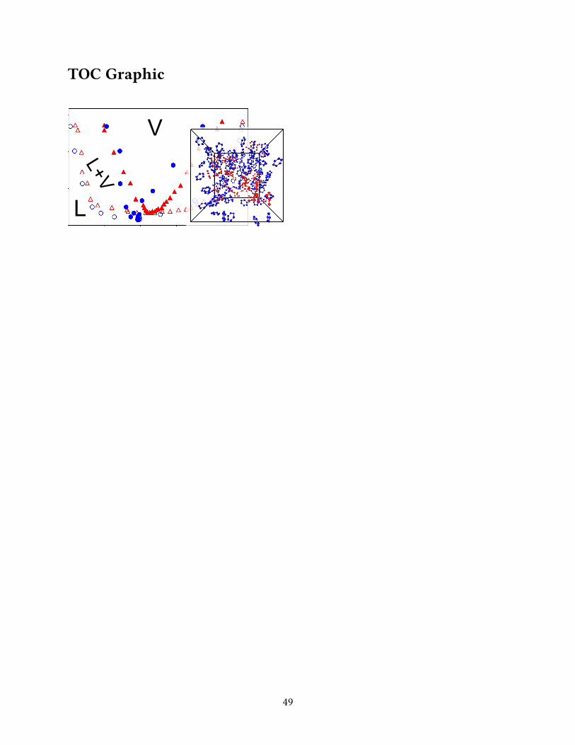
TOC Graphic

V

L

L+V

49