models of competition between one for-profit and one nonprofit firm
TRANSCRIPT

240
Charles University Center for Economic Research and Graduate Education
Academy of Sciences of the Czech Republic Economics Institute
Petra Brhlikova
Models of competition between one for-profit and one nonprofit firm
CERGE-EI
WORKING PAPER SERIES (ISSN 1211-3298) Electronic Version

Models of competition between
one for-profit and one nonprofit firm∗
Petra Brhlikova †
Abstract
To study the coexistence of two different ownership forms within anindustry, I develop a simple model of competition between one for-profit and one nonprofit firm. The two firms have different objectivesand face different constraints due to their choice of ownership sta-tus. Assuming heterogenous consumers I derive quality-price bundlesprovided by the two firms and their market shares under various con-ditions.
Pro analyzu koexistence dvou ruznych vlastnickych forem v ramci jed-noho sektoru vytvarım model souteze mezi jednou ziskovou a jednouneziskovou firmou. Tyto firmy majı ruzne ucelove funkce a platı pro neruzna omezenı. Za predpokladu heterogennıch spotrebitelu odvozujikvalitu a cenu produktu dodavanych danymi firmami a jejich podıl natrhu.
Keywords: Nonprofit firm, for-profit firm, monopoly, duopoly, mixedindustryJEL Classification: L31, L1, D42, D43
∗I would like to thank Marc Bilodeau, Andreas Ortmann, Avner Shaked, and RichardSteinberg for helpful comments. This research was started during a mobility stay at IUPUIEconomics Department, whose support is gratefully acknowledged.
†CERGE-EI, Charles University, Prague and the Academy of Sciences of the CzechRepublic, P.O.Box 882, Politickych veznu 7, 11121 Prague 1, Czech Republic, phone:+420 224 005 227, e-mail: [email protected].
Contents
1 Introduction 4
2 Model 7
2.1 Monopoly . . . . . . . . . . . . . . . . . . . . . . . . . . . . . 10
2.1.1 For-profit (FP) monopoly . . . . . . . . . . . . . . . . 11
2.1.2 Nonprofit (NP) monopoly . . . . . . . . . . . . . . . . 12
2.1.3 Comparison: FP versus NP monopoly . . . . . . . . . 13
2.2 Duopoly . . . . . . . . . . . . . . . . . . . . . . . . . . . . . . 13
2.2.1 FP duopoly - simultaneous choice . . . . . . . . . . . . 15
2.2.2 FP duopoly - sequential choice . . . . . . . . . . . . . . 16
2.2.3 Comparison: FP duopoly - simultaneous vs. sequential
choice . . . . . . . . . . . . . . . . . . . . . . . . . . . 17
2.2.4 NP duopoly - simultaneous choice . . . . . . . . . . . . 18
2.2.5 NP duopoly - sequential choice . . . . . . . . . . . . . 20
2.2.6 Comparison: NP duopoly - simultaneous vs. sequen-tial choice . . . . . . . . . . . . . . . . . . . . . . . . . 20
2.2.7 Comparison: FP versus NP duopoly . . . . . . . . . . 20
2.2.8 Mixed duopoly - simultaneous choice . . . . . . . . . . 21
2.2.9 Mixed duopoly - sequential choice . . . . . . . . . . . . 23
2.2.10 Comparison: mixed duopoly - simultaneous vs. se-quential choice . . . . . . . . . . . . . . . . . . . . . . 24
2.2.11 Comparison: mixed duopoly vs. FP and NP duopoly . 25
3 Discussion 27
3.1 Inefficiency in the NP firm . . . . . . . . . . . . . . . . . . . . 27
3.2 Market size . . . . . . . . . . . . . . . . . . . . . . . . . . . . 28
3.3 Mixed duopoly - modified sequential game . . . . . . . . . . . 29
4 Conclusion 32
5 References 34
6 Appendix 36
6.1 FP and NP monopoly . . . . . . . . . . . . . . . . . . . . . . 36
6.2 FP duopoly - simultaneous choice . . . . . . . . . . . . . . . . 36
6.3 FP duopoly - sequential choice . . . . . . . . . . . . . . . . . . 37
6.4 NP duopoly - simultaneous choice . . . . . . . . . . . . . . . . 38
6.5 NP duopoly - sequential choice . . . . . . . . . . . . . . . . . 39
6.6 Mixed duopoly - simultaneous choice . . . . . . . . . . . . . . 40
6.7 Mixed duopoly - sequential choice . . . . . . . . . . . . . . . . 42
6.8 Mixed duopoly - modified sequential game . . . . . . . . . . . 43

1 Introduction
The focus of this paper is competition between nonprofit and for-profit firms,
i.e. firms characterized by different ownership forms. The coexistence of
nonprofit and for-profit firms is common in many service industries such as
health care, education, theatrical production, orchestras, as well as sport
and recreational clubs (Rose-Ackerman 1996). Although the theoretical and
empirical research analyzes the distinctive nature and performance of these
two types of firms, usually it treats them separately, ignoring the interaction
between their production decisions.1
Nonprofit organizations are given several advantages including exemption
from paying certain taxes and regulatory breaks (Facchina et al. 1993).
They can, moreover, receive donations that have the effect of subsidies. In
return, nonprofits, through non-distribution and reasonable compensation
constraints, may not distribute profits to managers. Instead, they are ex-
pected to use their profits for enhancing quality or lowering price. In the
present paper I focus on quality enhancements although I also discuss cases
when a nonprofit firm decreases price to increase its market share.
Interestingly, nonprofits coexist and compete with their for-profit counter-
parts in fields such as health care, education, museums, and theatrical pro-
1A theoretical model by Hirth (1999) and recent empirical research on the competi-tion in health care (e.g., Grabowski and Hirth 2003, Kessler and McClellan 2001) areexceptions.
4

duction. The dominant theory of nonprofits, formulated by Hansmann (1980),
says that nonprofit organizations are an institutional response to information
asymmetries in markets where quality and effort are adjustable. Because of
the nondistribution and reasonable compensation constraints, nonprofits do
not have incentives to exploit market asymmetries. They, therefore, deliver
higher quality than their for-profit counterparts.
Based on the information asymmetry framework, Hirth (1999) builds a model
of competition between for-profit and nonprofit nursing homes. He focuses
on markets where the quality of care is either high or low. Consumers have
identical preferences for the quality of care and want to purchase only high
quality. Consumers, however, differ in the information they have about the
quality of care delivered by a particular provider. Informed consumers ob-
serve both quality and price, while uninformed consumers know only price
and the ownership form of a provider (nonprofit or for-profit). There are two
types of nonprofit firms, honest and so-called ‘for-profits-in-disguise’.2 Hirth
analyzes equilibria under three different levels of enforcement of the non-
distribution constraint. In the equilibrium with strict enforcement (which
is my focus here), uninformed consumers patronize nonprofit homes, which
deliver higher quality and charge a higher price than for-profit homes.3
2The term ‘for-profit-in-disguise’ was introduced by Weisbrod (1988) to represent profit-motivated entrepreneurs who enter the nonprofit sector to exploit the advantages bestowedon nonprofit institutions.
3For specific values of parameters it is even possible that the quality produced in thefor-profit sector equals the quality of nonprofit products but the price of the for-profitproduct is lower than the price of nonprofit product. Hirth also analyzes situations whenthe non-distribution constraint is moderately or weakly enforced. In such cases nonprofit
5

The empirical evidence does not support the suggested sorting of poorly in-
formed consumers into the nonprofit sector (Grabowski and Hirth 2003, Ort-
mann and Schlesinger 2003). The evidence in Clotfelter (1992), for example,
seems to favor the heterogeneous tastes story (Weisbrod 1975). According to
this theory, nonprofits emerge in situations when the market and the state fail
to deliver the whole spectrum of quality demanded. In the present study, I
build on the heterogeneous tastes story and analyze a full information model.
Hirth (1999) sketches a full information model where consumers have different
preferences for quality. Nonprofit firms choose a market niche corresponding
to their objectives, leaving the residual demand to for-profit firms. Specif-
ically, if nonprofits want to deliver high quality, for-profit firms would take
the low quality niche. Hirth suggests that if nonprofits would be eliminated,
for-profit firms would replace them, still providing the optimal quality spec-
trum. However, this is not true if the costs of producing high quality are
too high. The model presented here shows that for-profit firms might not be
willing to produce as high a quality as nonprofit firms would.
Monopolistic competition between identical for-profit firms was studied by
Shaked and Sutton (1982), among others. I analyze competition between
for-profit and nonprofit firms. Throughout the paper I assume positive pro-
duction costs that are independent of quantity and monotonically increasing
in quality.4 The cost functions of for-profits and nonprofits are identical.
status signals trustworthiness only under certain conditions or not at all.4The possibility of introducing variable costs of quantity is discussed below.
6
Given these cost configurations, I answer the following questions: How do
differences in objectives and constraints affect quality-price pairs supplied by
competing firms? What are the market shares of competing firms?
The structure of the paper is as follows. To better understand the impact of
different objectives for product price and quality I discuss first the two cases
with only one firm in the market: a single for-profit firm and a single non-
profit firm (Section 2.1). Then I proceed with models of duopoly, for-profit
versus for-profit firm (Section 2.2.1-3), nonprofit versus nonprofit firm (Sec-
tion 2.2.4-2.2.7), and finally mixed industry (Section 2.2.8-11). For duopoly
cases two different structures of the game are analyzed. In sequential choice
firms first choose quality of production and then decide the price. In simul-
taneous choice, both firms choose their prices and qualities at the same time.
In the third section, I summarize the results obtained and discuss several
generalizations of the model. The fourth section concludes. Computational
details are described in the Appendix.
2 Model
The demand side is populated by a continuum of heterogeneous consumers.
Specifically, consumers differ in their taste for quality, although they have
the same wealth, w. Consumers can consume two goods: a public good and a
private good. The public good is assumed to be a nonrival excludable public
7

good (a play, concert, art exhibition, etc.) and is provided by the nonprofit
firm or the for-profit firm, or both. It is characterized by quality, q, and
price, p ≤ w. Consumers differ in their preferences for the quality of the
public good. Their heterogeneity is modelled by a taste parameter, θ, that is
uniformly distributed over the interval 〈0, 1〉. According to their preferences
consumers buy one or zero (non-buying option) units of the public good.
The private good can be purchased outside the market of our interest. It is
characterized by quantity, x, and its price, px, is set equal to one. The utility
function, Ui(θiq, x) = θiq+x, is increasing in the consumption of both goods,
public and private.
Consumer i’s optimization problem is
Maxj,xθiqj + x s.t. pj + x = w,
where j = n, f, z stands for the (q, p)-bundles offered. The nonprofit firm
offers (qn, pn), the for-profit firm produces (qf , pf), and (qz, pz) = (0, 0) rep-
resents the non-buying option (denoted by z as a zero quality). Note that
consumers do not choose along a continuous budget constraint, but are of-
fered only three (q, p)-bundles to choose from (see Figure 1). The for-profit
and nonprofit bundle is determined by firms’ maximization problems de-
scribed below.
The public good, as mentioned, is supplied by the nonprofit (NP) and for-
profit (FP) firm. The NP firm is assumed to maximize quality and is re-
8

x
q
w
(qz, w − pz)
(qf , w − pf)
(qn, w − pn)
Figure 1: The three quality-price bundles offered
stricted from distributing profits.5 This means that the NP firm invests its
profits in further quality enhancement or alternatively, decreases price to in-
crease its market share. The realization of profits and investments in quality
or price subsidization happen in the same period, i.e. the NP firm, in fact,
faces a zero-profit constraint. The FP firm maximizes profit.
The costs of producing the public good are described by c(q), which is an
increasing function in q with increasing MC (i.e. it is convex in q). As
mentioned, the public good is assumed to be an excludable and nonrival good
whose costs are independent of the number of consumers. I.e. the costs, c(q),
incurred are in fact the fixed costs of producing quality q. For the NP firm’s
production costs I assume that all the advantages mentioned (tax exemption,
5An alternative objective function of the NP firm is a combination of quality andquantity (Newhouse 1970) or as in Hansmann (1981), who focuses on art performingfirms, quality, audience, or budget maximization. The focus of the present paper is qualitymaximization, although equilibrium for a more general case when the NP firm maximizesa linear combination of quality and quantity is also discussed.
9
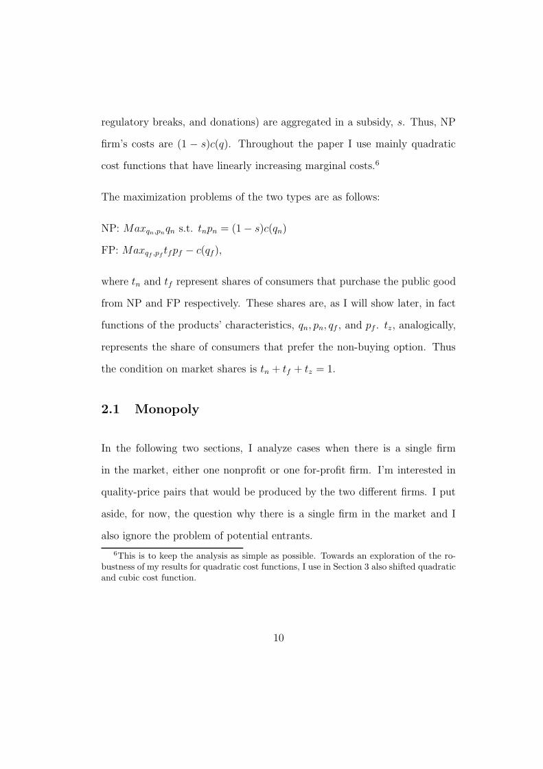
regulatory breaks, and donations) are aggregated in a subsidy, s. Thus, NP
firm’s costs are (1 − s)c(q). Throughout the paper I use mainly quadratic
cost functions that have linearly increasing marginal costs.6
The maximization problems of the two types are as follows:
NP: Maxqn,pnqn s.t. tnpn = (1 − s)c(qn)
FP: Maxqf ,pftfpf − c(qf),
where tn and tf represent shares of consumers that purchase the public good
from NP and FP respectively. These shares are, as I will show later, in fact
functions of the products’ characteristics, qn, pn, qf , and pf . tz, analogically,
represents the share of consumers that prefer the non-buying option. Thus
the condition on market shares is tn + tf + tz = 1.
2.1 Monopoly
In the following two sections, I analyze cases when there is a single firm
in the market, either one nonprofit or one for-profit firm. I’m interested in
quality-price pairs that would be produced by the two different firms. I put
aside, for now, the question why there is a single firm in the market and I
also ignore the problem of potential entrants.
6This is to keep the analysis as simple as possible. Towards an exploration of the ro-bustness of my results for quadratic cost functions, I use in Section 3 also shifted quadraticand cubic cost function.
10

2.1.1 For-profit (FP) monopoly
In this section I study the case when only the FP product and the non-buying
option, (qz, pz), are available to consumers. To determine demand for the FP
product we need to characterize a pivotal consumer, i.e. the consumer who
is indifferent between consuming the FP product and not buying the public
good at all. Formally, U(θqf , w − pf) = U(θqz, w − pz). Using the utility
function specified above, this equation characterizes the pivotal consumer
through her taste parameter, θ =pf
qf.
The FP firm supplies its product to all consumers with a sensitivity param-
eter of at least θ, and its market share is 1− pf
qf. The FP firm chooses qf and
pf to optimize
Maxqf ,pf(1 − pf
qf)pf − q2
f .
The FP firm chooses quality such that MR = MC and price such that
MR = 0. The solution to this problem, given the assumption on uniformly
distributed tastes for quality, is (qf , pf) = (0.1250, 0.0625). The FP firm
supplies its product to the upper segment of the market and serves one half
of the market, i.e. consumers with a sensitivity parameter of at least 1/2.
The profit of the FP firm is 0.0156.
11

2.1.2 Nonprofit (NP) monopoly
In this case consumers opt between the NP bundle, (qn, pn), and the non-
buying option. The pivotal consumer is characterized by θ = pn
qn.
The NP’s market share is 1 − θ = 1 − pn
qn. The NP firm chooses the (qn,pn)-
pair that maximizes quality given the nondistribution constraint:
(1 − pn
qn)pn = (1 − s)q2
n.
The solution for the NP firm’s maximization problem, given the assumption
on uniformly distributed tastes for quality, is (qn, pn) = ( 14(1−s)
, 18(1−s)
) with
(qn, pn) = (0.2500, 0.1250) for s = 0. Both qn and pn are increasing in s.
For all s ∈ 〈0, 1〉 the NP firm serves half of the market (the upper segment),
i.e. consumers with θi ≥ 1/2 buy the NP product while those who value the
quality of the public good less prefer the non-buying option.
With the NP firm maximizing a linear combination of quality and market
share, i.e. maxqn,pnbqn + (1 − b)(1 − pn
qn) s.t. (1 − pn
qn)pn = (1 − s)q2
n, where
b ∈ 〈0, 1〉, an interior solution exists only for b ∈ (1/2, 1〉. For a lower weight
on quality maximization and a correspondingly higher weight on market share
maximization, there is only a corner solution (qn, pn) = (0, 0). Intuitively,
the market share of the NP firm is maximized at pn = 0 (in such a case
its market share equals 1). At zero price the NP firm’s revenue is zero for
any market share, thus to satisfy the zero profit constraint it can produce
only zero quality. When quality maximization becomes more important the
12

NP firm finances the production of higher quality by increasing its price. Its
market share, however, declines.7
2.1.3 Comparison: FP versus NP monopoly
Comparing the FP and NP monopoly outputs derived in the previous two
sections, both monopolies supply to the upper half of the market. The quality
delivered and price charged by the NP firm is, however, higher than in the FP
case. Specifically for s = 0 we have (qn, pn) = (2qf , 2pf). The nonprofit firm,
under the assumption of quality maximization, invests its potential profit
and available subsidies only into quality enhancement. It does not subsidize
price to increase market share. Conversely, for increased quality consumers’
willingness to pay is higher and the NP firm is able to increase price. If the
NP firm would also give positive weight to market share maximization, it
would start to subsidize price in order to increase market share.
2.2 Duopoly
In this section I proceed with analyzing firms’ choice of (q, p)-pairs when
there are two firms in the market. I start with competition between two
identical FP firms, then turn to the competition between two identical NP
firms, and finally focus on the coexistence of one FP and one NP firm. In
all three cases I analyze a one-stage game (“simultaneous choice”) and a
7Equilibria for s = 0 and b > 1/2 are presented in Section 6.1.
13
two-stage game (“sequential choice”). In the one-stage game, the two firms
simultaneously choose their qualities and prices. In the two-stage game firms
are assumed to choose qualities simultaneously in the first stage. In the
second stage they choose prices given optimal qualities. This seems to be
a reasonable assumption since price can be adjusted more easily than the
quality of production.
Independently of the ownership form of competing firms there are two dif-
ferent qualities at different prices provided (plus the non-buying option is
available) in the duopoly.8 The three bundles are similar to those depicted
in Figure 1 (the (qh, w − ph) bundle would replace the NP bundle from Fig-
ure 1 and the (ql, w − pl) bundle would replace the FP bundle). The market
is divided into three segments: consumers buying the high-quality product
(qh), consumers buying the low-quality product (ql), and consumers who do
not buy the public good at all (non-buying option).
The taste for quality is again assumed to be uniformly distributed. Then the
sensitivity parameter of the consumer indifferent between the high-quality
and low-quality product, θ, and of the consumer indifferent between the low
and zero quality, θ, are the following:
U(θqh, w − ph) = U(θql, w − pl) ⇒ θ = ph−pl
qh−ql
U(θql, w − pl) = U(θqz, w − pz) ⇒ θ = pl−pz
ql−qz= pl
ql.
The market share of the high-quality producer is, therefore, th = 1−θ and the
8The reasoning why this is so for all types of duopolies studied here is given in othersections.
14

low-quality producer supplies a tl = (θ − θ)-fraction of the market. The rest
of the consumers, θ, prefer the non-buying option to both the high-quality
and low-quality products.
2.2.1 FP duopoly - simultaneous choice
The two FP firms simultaneously choose quality and price to maximize their
profits. Their optimization problems are as follows:9
FPh: maxqh,ph(1 − ph−pl
qh−ql)ph − q2
h
FPl: maxql,pl(ph−pl
qh−ql− pl
ql)pl − q2
l .
Note that in equilibrium the two FP producers offer different qualities at
different prices. Producing the same quality and charging equal prices can
not be an equilibrium since both producers have incentives either to slightly
increase quality or slightly decrease price in order to gain all the consumers
who want to purchase the public good. Producing the same quality and
charging different prices (or alternatively offering different qualities at a single
price) is not optimal for the producer with a higher price (or lower quality),
who earns zero or negative profit (zero revenue while costs are greater than
or equal to zero). Thus, two FP firms offer two different qualities at different
prices, i.e. enjoy a locally monopolistic position and earn positive profits.
9In this problem I assume that the market size is 1. In Section 6, I derive a solution toa more general problem, where a positive parameter a represents the market size.
15

The equilibrium is (qh, ql, ph, pl) = (0.12, 0.04, 0.05, 0.01).10 Correspond-
ing market shares and profits are: th = 0.54, tl = 0.27, Πh = 0.01, and
Πl = 0.0005. Thus the firm producing high quality delivers slightly lower
quality and charges a lower price than the FP monopoly. It, however, serves
more than one half of the market while the FP and NP monopolies serve
exactly one half of the market. The firm producing low quality serves more
than one quarter of the market. The two firms do not supply to the whole
market, because a positive share of consumers prefers the non-buying option
to products offered by the two firms.11 Both firms earn positive profits.
2.2.2 FP duopoly - sequential choice
In this section it is assumed that producers decide about their choice variables
in two stages. First they simultaneously choose qualities to maximize their
profits. Then, given optimal qualities, they choose optimal prices.
Similarly to the simultaneous choice, different qualities and different prices
are chosen by the two FP firms. The choice of the same quality would lead
to Bertrand competition in the second stage. As a result firms would earn
negative profits equal to fixed costs. If they choose different qualities, profits
10First order conditions and the analytical solution are in Section 6. In the case of theFP duopoly, the simultaneous choice and also the sequential choice have two asymmet-ric equilibria in which one or the other firm produces high quality. There exists also asymmetric equilibrium that I do not specify here, in which the two firms play a mixedstrategy.
11In Shaked and Sutton (1982) the two top firms cover the whole market since theconsumer with the lowest taste for quality has strictly positive preferences for quality.
16
are strictly positive. The choice of the same price when qualities are different
is not optimal since the firm with lower quality loses all its customers.
To solve the problem I start by analyzing the second stage - simultaneous
choice of optimal prices. Given optimal qh and ql producers set prices to
optimize profits:
FPh: maxph(1 − ph−pl
qh−ql) − q2
h
FPl: maxpl(ph−pl
qh−ql− pl
ql) − q2
l .
This is equivalent to optimizing their revenues since production costs are
treated as constant at this stage (fixed costs of producing a certain quality
level). Optimal prices are p∗h(qh, ql) = 2qh(qh−ql)
4qh−qland p∗l (qh, ql) = ql(qh−ql)
4qh−ql.12
In the first stage, producers choose optimal qualities given optimal prices
p∗h(qh, ql) and p∗l (qh, ql):
FPh: maxqh
4q2
h(qh−ql)
(4qh−ql)2− q2
h
FPl: maxql
qhql(qh−ql)(4qh−ql)2
− q2l .
The equilibrium is (qh, ql, ph, pl) = (0.13, 0.02, 0.05, 0.01), with th = 0.53, tl =
0.26, Πh = 0.01, and Πl = 0.0008.
2.2.3 Comparison: FP duopoly - simultaneous vs. sequentialchoice
Table 1 summarizes the results of the two previous sections
12See Section 6 for computational details.
17

Choice qh ql ph pl th tl Πh Πl
sim 0.1242 0.0364 0.0474 0.0069 0.5395 0.2698 0.0101 0.0005seq 0.1267 0.0241 0.0538 0.0051 0.5250 0.2625 0.0122 0.0008
Table 1: FP duopoly - simultaneous and sequential choice
The two FP firms are better off when they optimize the choice of quality
and price in two stages. Prices are chosen in the same way in both cases
but there is larger quality differentiation in the sequential game. The market
share served in the sequential game is smaller than in the simultaneous game
and profits earned by the two firms are higher. This is due to the additional
information the firms have about qualities actually chosen in the first stage.
Knowing that they have an opportunity to adjust prices to the chosen qual-
ities in the second stage firms choose a better ‘location’ in the market in the
first stage. The optimal ‘location’ choice corresponds to maximal differentia-
tion. It increases the monopolistic power of the two firms in their ‘locations’
and firms can exploit consumers’ willingness to pay.
2.2.4 NP duopoly - simultaneous choice
Similarly to the FP duopoly in Section 2.2.1, the two NP firms simultaneously
choose their qualities and prices. The NP’s objective is quality maximization
rather than profit maximization. The NP firms, in addition, face the zero
profit constraint. The qualities offered by the two NP firms are expected to
be, therefore, higher than qualities produced by two FP firms. This is true
18

even in the case of zero subsidy.13 Optimization problems of the two NP
firms are as follows
NPh: maxqh,phqh s.t. (1 − ph−pl
qh−ql)ph = q2
h
NPl: maxql,plql s.t. (ph−pl
qh−ql− pl
ql)pl = q2
l .
As in the FP duopoly, two different qualities at different prices are produced
by two NP firms. Rather than profit, the NP firms maximize the quality of
their products. The quality offered by the NP monopoly is not feasible when
there are two NP firms. The production costs of two units of such a high
quality are twice as high as the production costs of one unit, while the revenue
is the same. This means negative profits for both NP firms. A quality they
could together produce is half of that produced by the NP monopoly. It can
not be, however, the equilibrium outcome since both firms have an incentive
to increase price that corresponds to higher quality. Thus, two NP firms, like
FP firms, produce two different qualities and charge different prices.
Specifically, the equilibrium is (qh, ql, ph, pl) = (0.2133, 0.0533, 0.0853, 0.0107).14
13In this section I assume that s = 0. A strictly positive subsidy would lead to higherqualities offered by the two firms. They are, however, expected to proportionally movetoward higher quality if they have the same cost structure. In reality, it might be the casethat s is different for the two NP firms. For instance, the NP firm producing high qualitymost probably receives larger donations because consumers preferring high quality havehigher willingness to pay while they pay a price equal to the willingness to pay of thepivotal consumer. Hansmann (1981) argues that a big part of contributions is receivedfrom those who attend to performance. Donations then correspond to voluntary pricediscrimination. This is true also for colleges and universities whose donations from alumnican be conceptualized as deferred fee payments. In the present paper I, nevertheless,ignore consumers’ opportunities to donate.
14Similarly to the FP duopoly, there are again two asymmetric equilibria with both firmsin the market, in which one or the other firm produces high quality and one symmetric
19

The corresponding market shares are th = 0.5333, tl = 0.2667, and profits of
the two firms are zero due to the zero profit constraint (Πh = Πl = 0).
2.2.5 NP duopoly - sequential choice
In sequential choice, NP firms first optimize with respect to quality and then,
knowing the optimal qualities, they choose prices. Prices are, however, au-
tomatically determined by qualities through the zero-profit constraint. NPs
in fact, have no choice in the second stage and sequential choice leads to the
same solution as simultaneous choice.15
2.2.6 Comparison: NP duopoly - simultaneous vs. sequentialchoice
The equilibria for simultaneous and sequential choice with two NP firms are
the same.
2.2.7 Comparison: FP versus NP duopoly
In the FP duopoly sequential choice leads to a larger quality differentiation.
In contrast, the quality differentiation is not attractive to two NP firms that
aim to maximize quality. Increasing the top quality means moving toward
equilibrium (not specified here) in which the NP firms play a mixed strategy. There are,however, two asymmetric equilibria with only one firm in the market, in which one or theother NP firm delivers the NP monopoly outcome.
15For completeness, first order conditions and analytical solution are in Section 6.5.
20
the NP monopoly output that does not allow a lower quality to exist in the
market.
In the NP duopoly, the qualities offered are higher than in the FP duopoly.16
The market share is slightly lower than in the FP case: 0.80 compared to
0.81.
2.2.8 Mixed duopoly - simultaneous choice
In the previous two sections I examined the segmentation of the market when
there are two producers of the same type. In this section I analyze the possible
coexistence of one NP and one FP firm within an industry. Recall that the
NP has to satisfy the nondistribution constraint (=zero-profit constraint)
and is assumed to maximize quality. In addition, the NP firm has a cost
advantage due to the availability of subsidies (tax exemption, regulatory
breaks, donations) stemming from its NP status. The FP firm is assumed to
maximize profit.
In the mixed duopoly it is not reasonable for the FP firm to choose the same
quality as the NP firm. Since the NP firm aims to break even, for the FP
firm to choose the same quality would imply zero (if s = 0) or negative (if
16To compare top the qualities in simultaneous choice of two FP firms to two NP firmsstarting from FP’s quality, the NP firm has to satisfy the zero profit constraint, thus itcan invest the FP’s profit (0.01) into quality enhancement. This allows it to increase qual-ity from 0.12 to approximately 0.16. The increased quality positively affects consumers’willingness to pay and the NP firm is able to increase price and thus enhance qualityfurther.
21

s > 0) profit. Moreover, similar to the NP duopoly case, the same quality
produced by two firms is significantly lower than the quality produced by
the NP monopoly. The NP firm in the mixed duopoly, therefore, has an
incentive to increase quality. Thus, two different qualities at different prices
are offered also in the mixed duopoly with the higher quality being provided
by the NP firm.
The above argument also rules out the case of the FP catering to the top
end of the market and the NP producing a lower quality. The FP firm would
produce the top quality only if it is a profitable option. The NP firm can,
however, produce the same quality at a lower price than the FP has to charge.
Alternatively, the NP firm can produce a higher quality than the FP firm at
a price equal to the FP price. In both cases, consumers previously served by
the FP firm would now prefer the NP product. The FP firm would be forced
to produce a lower quality than the NP firm.
The two maximization problems are the following:
NP: Maxqn,pnqn s.t. (1 − pn−pf
qn−qf)pn = (1 − s)q2
n
FP: Maxqf ,pf(
pn−pf
qn−qf− pf
qf)pf − q2
f .
First order conditions and a general solution can be found in Section 6.6.
Specifically, if s = 0, the two firms choose in equilibrium the following
qualities and prices: (qn, qf , pn, pf) = (0.2299, 0.0337, 0.1019, 0.0075). The
corresponding market shares and profits are tn = 0.5190, tf = 0.2595, and
22

Πn = 0, Πf = 0.0008.
2.2.9 Mixed duopoly - sequential choice
In this section I analyze the competition between one NP and one FP firm
when they decide about qualities and prices in two stages. First, they simul-
taneously choose qualities. Second, knowing the chosen quality levels, both
its own and the rival’s, they set prices. The FP firm maximizes profit in both
stages while the NP firm chooses optimal quality and then optimal price to
maximize quality such that the zero profit constraint is satisfied.17
Similarly to the simultaneous case, there are two different qualities offered
at different prices and the NP firm produces high quality while the FP firm
delivers low quality. Starting with the analysis of the second stage the two
maximization problems are as follows:
NP: Maxpnqn s.t. (1 − pn−pf
qn−qf)pn = (1 − s)q2
n
FP: Maxpf(
pn−pf
qn−qf− pf
qf)pf − q2
f .
Assuming that the NP’s constraint is binding the optimal prices are
p∗n(qn, qf) =2qn(qn−qf )
4qn−qfand p∗f (qn, qf) =
qf (qn−qf )
4qn−qf. Using the optimal prices in
the first stage the two firms solve
NP: Maxqnqn s.t. 4(qn − qf) = (1 − s)(4qn − qf)
2
17An alternative problem where the NP firm first maximizes quality (unconstrainedoptimization) and then chooses price satisfying the zero-profit constraint is discussed inSection 3.
23
FP: Maxqf
qnqf (qn−qf )
(4qn−qf )2− q2
f .
The equilibrium for s = 0 is (qn, qf , pn, pf ) = (0.2344, 0.0272, 0.1067, 0.0062).
The corresponding market shares and profits are tn = 0.5149, tf = 0.2575,
and Πn = 0, Πf = 0.0009.
2.2.10 Comparison: mixed duopoly - simultaneous vs. sequentialchoice
First, there is a smaller product differentiation in simultaneous choice than
in sequential choice in the mixed duopoly. Recall that larger differentiation
in the sequential game was present in the FP duopoly but impossible in the
NP duopoly. In the mixed duopoly, product differentiation coincides with
producers’ incentives since the NP firm wants to increase quality and the FP
firm wants to increase its profit. It can exploit consumers’ willingness to pay
more the more different the NP product is.
When one FP and one NP coexist, the NP firm produces quality (0.2299 in
simultaneous choice and 0.2344 in sequential choice) that is close to the NP
monopoly output (0.2500) and serves more than half of the market. The FP
firm provides much lower quality, serves slightly more than one quarter of
the market, and earns positive profit.
The equilibria for positive subsidy18 available to the NP firm and the case
18Equilibria for simultaneous choice are computed for s ∈ 〈0, 0.9〉 (see Section 6.6).The lowest values of subsidy (0.1 and 0.2) characterize commercial NP firms while highersubsidies characterize donative NP firms. Hansmann (1981, citing Baumol and Bowen
24

when the market size is doubled (i.e. a = 2) are shown in Section 6.6. A
positive subsidy means a comparative advantage for the NP firm, which is
able to produce a higher quality. The subsidy, however, also helps the FP
firm which is, after the NP’s move toward a higher quality, able to increase its
price and earn a higher profit. Note that the FP quality is decreasing with
the subsidy given to the NP firm. The FP firm wants to enlarge product
differentiation, which results in a higher profit.
2.2.11 Comparison: mixed duopoly vs. FP and NP duopoly
To emphasize the differences between quality-price bundles offered under
various combinations of ownership types Table 2 summarizes the equilibria
of simultaneous quality-price choices.
Type qh ql ph pl th tl Πh Πl
h = FP, l = FP 0.12 0.04 0.05 0.01 0.54 0.27 0.0101 0.0005h = NP, l = NP 0.21 0.05 0.09 0.01 0.53 0.27 0.0000 0.0000h = NP, l = FP 0.23 0.03 0.10 0.01 0.52 0.26 0.0000 0.0008
Table 2: FP duopoly, NP duopoly, and mixed duopoly
qh(ql) and ph(pl) represent high (low) quality and prices. th, tl, Πh and Πl
are corresponding market shares and profits. The left-most column describes
the duopoly type. For instance, (h = NP, l = FP ) represents the mixed
duopoly since the NP firm delivers high quality (h) and the FP firm delivers
low quality (l).
1968) reports that donations to art performing groups stand for between one-third andone-half of their income.
25

We can see that the market shares of the firms catering to the upper and
lower end of the market are very similar across different combinations of
ownership types: 0.52− 0.54 for the top product and 0.26− 0.27 for the low
quality product. There are, however, large differences in qualities produced
and prices charged. In the FP duopoly the top quality (0.12) is significantly
lower when compared to the other two cases (0.21 in the NP duopoly and
0.23 in the mixed duopoly). Surprisingly, the competition between a FP
and NP firm leads to a higher top quality than in the case of two NP firms.
This can be explained by the attempt of the top firm to decrease its quality
when the low quality increases.19 I.e. if the competition is tougher (as in
the case of two NP firms, or when firms decide simultaneously compared to
sequentially), the top quality is lower so as to offer more competitive quality-
price bundles and in this way to protect its market share. If the NP firm
competes with a FP firm, the NP firm does not decrease quality as much as
in the case of two NP firms since the low quality offered by the FP rival is
lower than the low quality produced by the NP competitor. The FP firm,
in addition, maximizes profit, whaich means that the competition for the
marginal consumer is not as tough as in case of the zero-profit competitor.
19This is true for sequential choice when the NP competes with the FP.
26

3 Discussion
In the preceding sections, I analyzed the coexistence of one NP and one FP
firm within a market. The two firms choose simultaneously or sequentially
qualities and prices. The choice of each firm affects its own but also the rival’s
market share. In the following subsections I discuss several generalizations
and extensions of the mixed duopoly model discussed in Section 2.2.8.
3.1 Inefficiency in the NP firm
It is often argued that tax-exemption, donations, and lack of owners lower
pressure on the NP’s competitiveness and create an opportunity for ineffi-
ciency in NP firms (Newhouse 1970, Rose-Ackerman 1996). To analyze the
impact of NP inefficiency on (q, p)-pairs offered by the FP and NP firm I
assume the subsidy, s, to be negative. In such case the NP firm has a com-
parative disadvantage introduced through higher production costs.
In reality, the NP firm even with s ≥ 0 might be inefficient. For instance,
take donations and tax exemption that could decrease production costs by
0.7. Due to an inefficiency in the NP firm, the effect of these advantages
might be only 0.9.
In Table 3 I compare the equilibrium with s = 0.3 to equilibria with s ∈
〈−0.3, 0.0〉.
27
s qn qf pn pf tn tf Πn Πf
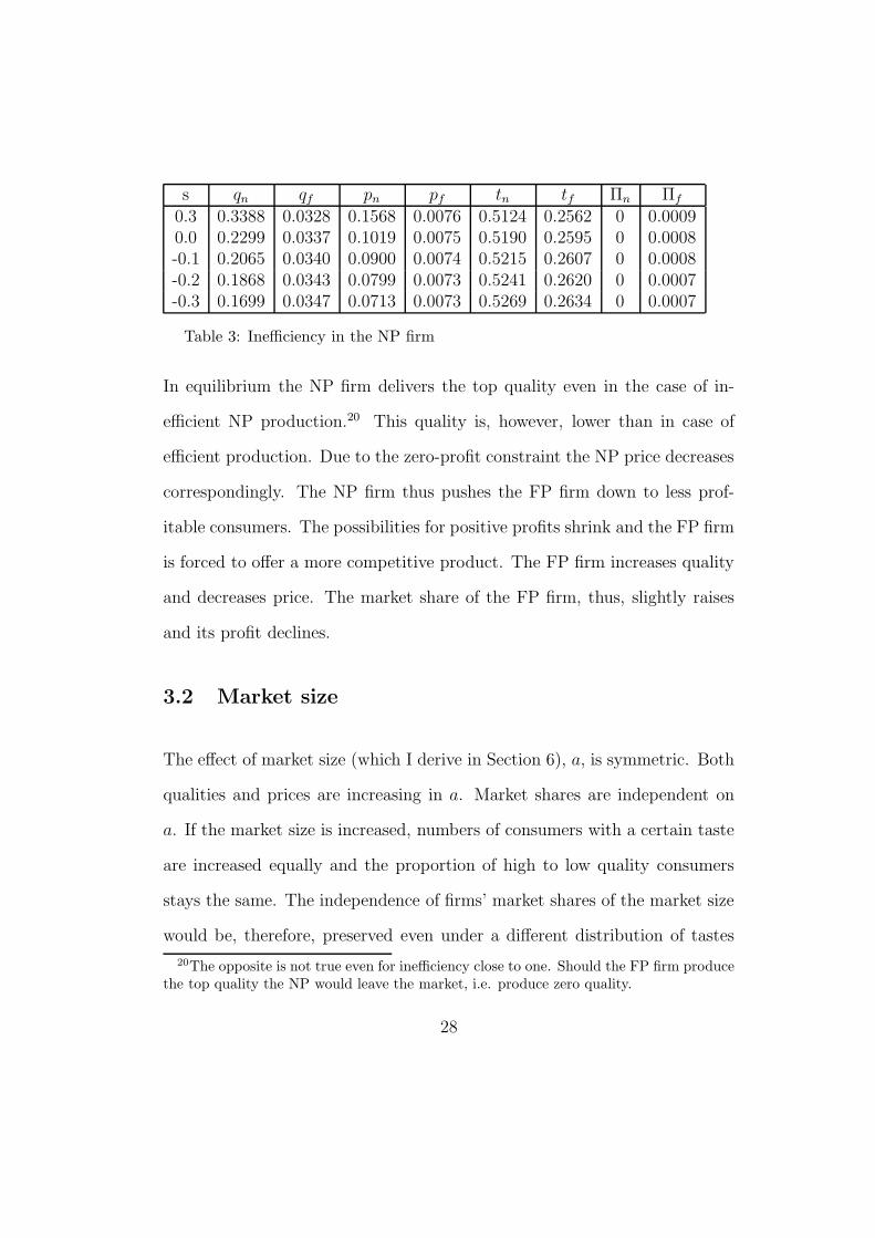
0.3 0.3388 0.0328 0.1568 0.0076 0.5124 0.2562 0 0.00090.0 0.2299 0.0337 0.1019 0.0075 0.5190 0.2595 0 0.0008-0.1 0.2065 0.0340 0.0900 0.0074 0.5215 0.2607 0 0.0008-0.2 0.1868 0.0343 0.0799 0.0073 0.5241 0.2620 0 0.0007-0.3 0.1699 0.0347 0.0713 0.0073 0.5269 0.2634 0 0.0007
Table 3: Inefficiency in the NP firm
In equilibrium the NP firm delivers the top quality even in the case of in-
efficient NP production.20 This quality is, however, lower than in case of
efficient production. Due to the zero-profit constraint the NP price decreases
correspondingly. The NP firm thus pushes the FP firm down to less prof-
itable consumers. The possibilities for positive profits shrink and the FP firm
is forced to offer a more competitive product. The FP firm increases quality
and decreases price. The market share of the FP firm, thus, slightly raises
and its profit declines.
3.2 Market size
The effect of market size (which I derive in Section 6), a, is symmetric. Both
qualities and prices are increasing in a. Market shares are independent on
a. If the market size is increased, numbers of consumers with a certain taste
are increased equally and the proportion of high to low quality consumers
stays the same. The independence of firms’ market shares of the market size
would be, therefore, preserved even under a different distribution of tastes
20The opposite is not true even for inefficiency close to one. Should the FP firm producethe top quality the NP would leave the market, i.e. produce zero quality.
28

for quality.
3.3 Mixed duopoly - modified sequential game
In mixed duopoly - sequential choice (Section 2.2.9), I assumed that the NP
firm maximizes quality in both stages such that the zero-profit constraint is
satisfied. In the first stage its control variable is quality and in the second
stage its price. It might be reasonable to take an alternative sequential prob-
lem where the NP firm maximizes quality first (without explicit constraints)
and then chooses its price just to cover its fixed costs (in what follows I use
the term ‘modified sequential game’). These two setups are, indeed, differ-
ent since in the first case the NP firm maximizes quality with respect to
both its variables, quality, and price, while in the modified sequential game
it maximizes quality only with respect to quality.
Thus, while the FP firm maximizes profit in both stages, the NP firm first
maximizes quality and then it sets price such that the zero-profit constraint
is satisfied.
Starting with the second stage, the FP firm chooses a price that maximizes its
profit (i.e. sets MR = 0) given qn, qf and pn. Its pricing strategy follows the
pricing strategy of the NP firm (pf =pnqf
2qn). Thus, if the NP firm charges a
higher price then the FP firm can also charge a higher price to gain consumers
with a higher willingness to pay. On the other hand if the NP charges a lower
29

price, then the FP has to charge a proportionately lower price.21
The NP firm, given qn, qf and pf , charges price pn which satisfies the zero-
profit constraint. There are two such prices since the constraint is quadratic
in pn. With a lower price, the NP firm produces lower quality and enlarges
its market share. With a higher price, it becomes attractive to a smaller
number of consumers. On the other hand, these consumers are willing to
pay more and the firm even might be able to increase quality. The smaller
market share is thus compensated for by higher price and the NP firm is still
able to cover its production costs.
In the first stage of the modified sequential game, the NP firm maximizes
quality given p∗n(qn, qf), p∗f(qn, qf) and qf . The FP firm chooses quality to
maximize its profit.
In the modified sequential game, surprisingly, the coexistence of the two firms
is not possible in equilibrium. The nonprofit firm chooses monopoly quality,
14(1−s)
. Such qn ensures that the FP firm stays out of the market. This is
indeed optimal for the NP firm since with the entry of the FP firm it would
need to decrease its quality which is against its goal to maximize quality.22
The fact that the FP firm cannot profitably enter is striking since the NP
firm satisfies only one half of the market.23 From the FP firm point of view
21For computational details see Section 6.22This can be checked differentiating the NP’s best response to the FP’s quality. The
derivative is decreasing; see Section 6 for details.23For instance in the Shaked and Sutton (1982) model with zero costs and symmetric
producers the whole market is satisfied.
30
the NP firm is too tough a rival to compete with since it has zero profit.
In the modified sequential game, the coexistence is not possible even if we
keep the costs of quality equal to zero up to a certain point (d > 0) and then
let them grow quadratically. This is curious since zero costs for qualities up
to d should allow the FP firm to enter and even make a positive profit. This
is, indeed, the result of the simultaneous game, where the equilibrium for
s = 0 and d = 0.25 is (qn, qf , pn, pf) = (0.5659, 0.2500, 0.1776, 0.0392). The
corresponding market shares and profits are tn = 0.5621, tf = 0.2810, and
Πn = 0.0000, Πf = 0.0110.
The shifted quadratic cost function allows the quality of 0.25 to be produced
at zero cost, thus the NP firm can produce significantly higher quality than
previously (Section 2.2.9). Consumers’ willingness to pay increases. The
NP firm can charge a higher price and subsequently increase its quality even
further (0.5659 compared to 0.2344 for the case of a non-shifted quadratic
cost function). The FP firm produces a quality of 0.25 at zero cost. Thus it
can decrease its price to gain larger market share. The profit of the NP firm
increases to 0.0110 (from 0.0008).
For a shifted cubic function of the form c(q) = (q − d)3 + d3, where d =
0.25, the results are reversed compared to the case of the shifted quadratic
cost function. There exists an equilibrium with both firms in the market in
the modified sequential game but such an equilibrium does not exist in the
simultaneous game.
31
4 Conclusion
The coexistence of NP and FP firms within an industry is common in many
service fields. There is, however, a lack of theoretical and empirical studies
that focus on interaction between firms that have adopted these different
ownership forms. In this paper, I develop a simple model of competition
between one NP and one FP firm. The two firms have different objectives
and face different constraints. I derive optimal quality-price bundles chosen
by the two firms and their market shares.
The present model extends models of vertical differentiation to the possibility
of one firm being NP. It also extends the research on the cross-sectoral com-
petition between NP and FP firms in that I focus on quality as the strategic
variable.
Under the assumption of heterogeneous tastes for quality the quality maxi-
mizing NP firm always produces the top quality in the market. The NP firm
sells its product to the upper segment of the market and serves slightly more
than one half of it. The FP firm serves consumers with a lower willingness
to pay and its market share is slightly above one quarter.
Since the NP firm can receive subsidies, their impact on equilibrium outcomes
is discussed. Subsidies decrease production costs of the NP firm and cause an
increase in quality and price of the NP product. The FP firm can decrease
the quality and price of its product in turn and its profit increases. Market
32

shares of both firms decline. The total market share served by the two firms,
therefore, decreases with the subsidy given to the NP firm.
The models presented here are based on specific assumptions. Although
Section 3 discusses some extensions (e.g. inefficiency in the NP firm) other
interesting questions remain unanswered.
First, in the present paper only fixed production costs are assumed: firms
have to attract a sufficient market share to cover the fixed costs of the quality
produced. Incorporating variable production costs would make the model
better suited for the analysis of the coexistence of FP and NP firms in health
care and education, where the variable cost component is non-negligible.
Second, in the present models I assumed that the NP firm maximizes qual-
ity. Quality maximization by the NP firm is a useful benchmark case since
it illustrates how large the product differentiation could be if two competing
firms have different objectives. In reality, NP firms have more complicated
objectives such as a combination of quality and market share maximization.
Also, I assumed that consumers are identical in wealth. With wealth differ-
ences it would be possible to explore objectives of the NP firm such as serving
indigents, a quid pro quo that constitutes a major rationale for various tax
and regulatory breaks bestowed on NPs.
Third, in the analysis I put aside the possibility of entry by an additional
firm. In the NP monopoly the entry of another firm, whether NP or FP, is
33

not possible. It would be interesting to explore whether a third firm could
enter the mixed duopoly or whether an entering NP firm could push the FP
firm out of the market.
5 References
Clotfelter, C.T. (1992). Who Benefits from the Nonprofit Sector? University
of Chicago Press, Chicago.
Facchina, B., Showell, E.A., and Stone, J.E. (1993). Privileges and exemp-
tions enjoyed by nonprofit organizations. University of San Francisco Law
Review 28, 85-121.
Grabowski, D.C. and Hirth, R.A. (2003). Competitive spillovers across non-
profit and for-profit nursing homes. Journal of Health Economics 22, 1-22.
Hansmann, H. (1980). The role of nonprofit enterprise. Yale Law Journal
89, 835-901.
Hansmann, H. (1981). Nonprofit enterprise in the performing arts. The Bell
Journal of Economics 12, 341-361.
Hirth, R.A. (1999). Consumer information and competition between non-
profit and for-profit nursing homes. Journal of Health Economics 18, 219-
240.
34
Leete, L. (2001). Whither the nonprofit differential? Estimates from the
1990 Census. Journal of Labor Economics 19(1), 136-170.
Kessler, D. and McClellan, M.B. (2001). The effects of hospital ownership
on medical productivity. NBER Working Paper No. 8537.
Newhouse, J.P. (1970). Toward a theory of nonprofit institutions: An eco-
nomic model of a hospital. American Economic Review 60(1), 64-74.
Ortmann, A. and Schlessinger, M. (2003). Trust, repute, and the role of
nonprofit enterprise. In The Study of Nonprofit Enterprise: Theories and
Approaches, eds. H.K. Anheier and A. Ben-Ner. New York, Kluwer.
Rose-Ackerman, S. (1996). Altruism, nonprofits, and economic theory. Jour-
nal of Economic Literature 34, 701-728.
Shaked, A. and Sutton, J. (1982). Relaxing price competition through prod-
uct differentiation. Review of Economic Studies 49, 3-13.
Weisbrod, B. (1975). Toward a theory of the voluntary nonprofit sector in a
three-sector economy. In Altruism, Morality, and Economic Theory, ed. E.S.
Phelps. New York, Russell Sage Foundation.
Weisbrod, B. (1988). The Nonprofit Economy. Harvard University Press,
Cambridge.
Williamson, O.E. (1963). Managerial discretion and business behavior. Amer-
35
ican Economic Review 53(5), 1032-1056.
6 Appendix
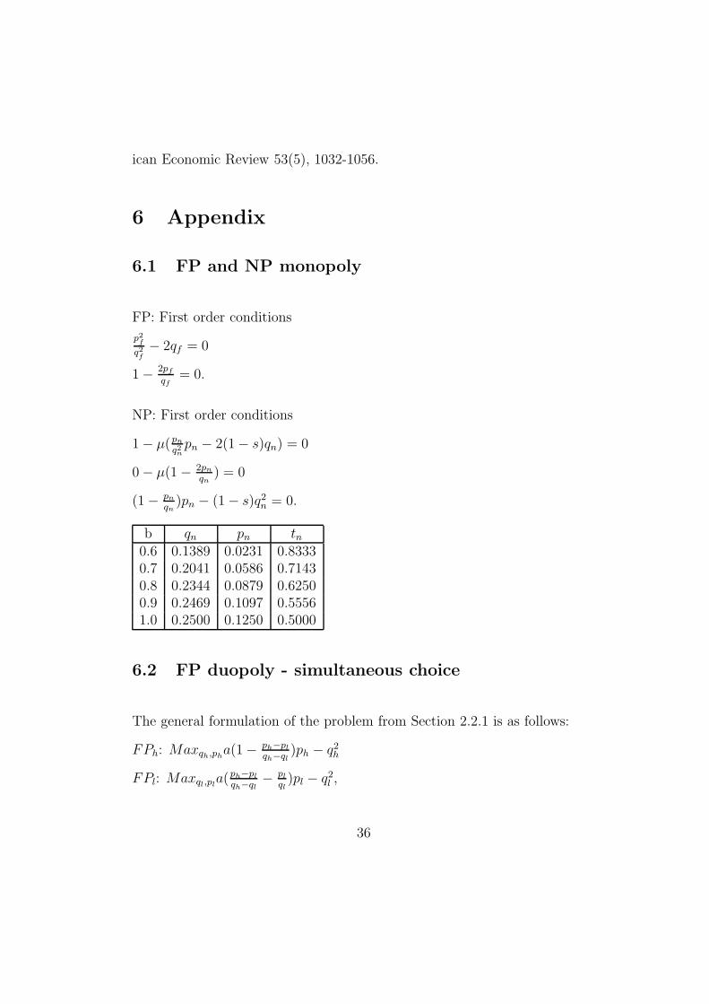
6.1 FP and NP monopoly
FP: First order conditions
p2
f
q2
f
− 2qf = 0
1 − 2pf
qf= 0.
NP: First order conditions
1 − µ(pn
q2npn − 2(1 − s)qn) = 0
0 − µ(1 − 2pn
qn) = 0
(1 − pn
qn)pn − (1 − s)q2
n = 0.
b qn pn tn0.6 0.1389 0.0231 0.83330.7 0.2041 0.0586 0.71430.8 0.2344 0.0879 0.62500.9 0.2469 0.1097 0.55561.0 0.2500 0.1250 0.5000
6.2 FP duopoly - simultaneous choice
The general formulation of the problem from Section 2.2.1 is as follows:
FPh: Maxqh,pha(1 − ph−pl
qh−ql)ph − q2
h
FPl: Maxql,pla(ph−pl
qh−ql− pl
ql)pl − q2
l ,
36

where the positive parameter a represents market size. The first order con-
ditions are the following:
ph − (qh − ql + pl)/2 = 0
aphph−pl
(qh−ql)2− 2qh = 0
pl − phql
2qh= 0
apl(ph−pl
(qh−ql)2+ pl
q2
l
) − 2ql = 0.
From the first and third equation we can write prices as functions of qualities
ph = 2qh(qh−ql)4qh−ql
, pl = ql(qh−ql)4qh−ql
,
where 4qh 6= ql. Plugging these expressions into the second and fourth equa-
tions we get the following system of two equations and two variables, qh and
ql:
a(2qh − ql) = (4qh − ql)2
aq2h = 2ql(4qh − ql)
2.
In equilibrium,
qh = a(26+7√
2)289
, ql = a(19−6√
2)289
, ph = 2a(364+387√
2)
4913(5+2√
2), pl = a(−23+250
√2)
4913(5+2√
2),
th = 2(364+387√
2)
1479+1343√
2, tl = 2272+5169
√2
11985+16643√
2, and
Πh = 2a3(366315+206587√
2)
83521(751+569√
2), Πl = a2(1720161−686644
√2)
83521(7441+6305√
2).
6.3 FP duopoly - sequential choice
Second stage - the choice of optimal prices
First order conditions to the problem in Section 2.2.2 are the following:
ph − (qh − ql + pl)/2 = 0
37

pl − phql
2qh= 0.
Solving the system we get p∗h(qh, ql) = 2qh(qh−ql)
4qh−qland p∗l (qh, ql) = ql(qh−ql)
4qh−ql.
First stage - the choice of optimal qualities
First order conditions are the following:
−32aq2
h(qh−ql)
(4qh−ql)3+
4aq2
h+8aqh(qh−ql)
(4qh−ql)2= 2qh
aqh(qh−ql)−aqhql
(4qh−ql)2+ 2aqhql(qh−ql)
(4qh−ql)3= 2ql.
6.4 NP duopoly - simultaneous choice
First order conditions to the maximization problem (2.2.5) are
1 + µ(−2qh + aph(ph−pl)(qh−ql)2
) = 0
µ(a(1 − ph−pl
qh−ql) − aph
qh−ql) = 0
−q2h + aph(1 − ph−pl
qh−ql) = 0
1 + ν(apl(ph−pl
(qh−ql)2+ pl
q2
l
) − 2ql) = 0
ν(apl(− 1qh−ql
− 1ql
) + a(ph−pl
qh−ql− pl
ql)) = 0
apl(ph−pl
qh−ql− pl
ql) − q2
l = 0.
From the first and fourth condition we see that µ and ν are non-zero. There-
fore the second and fifth equation can be rewritten as
a(1 − ph−pl
qh−ql) − aph
qh−ql= 0
apl(1
qh−ql+ 1
ql) − a(ph−pl
qh−ql− pl
ql) = 0.
From these two equation we have
ph = 2qh(qh−ql)4qh−ql
and pl = ql(qh−ql)4qh−ql
.
For qh and ql non-zero and 4qh 6= ql FOCs numbers 3 and 6 can be then
38

simplified to
4a(qh − ql) = (4qh − ql)2
aqh(qh − ql) = ql(4qh − ql)2.
The system can be solved for qh and ql and the equilibrium is
(qh, ql, ph, pl, th, tl, Πh, Πl) = (16a75
, 4a75
, 32a375
, 4a375
, 815
, 415
, 0, 0).
6.5 NP duopoly - sequential choice
The choice of price is
NPh: maxphqh s.t. (1 − ph−pl
qh−ql)ph = q2
h
NPl: maxplql s.t. (ph−pl
qh−ql− pl
ql)pl = q2
l .
First order conditions are
µ(a − aph−pl
qh−ql− a ph
qh−ql) = 0
a(1 − ph−pl
qh−ql)ph = q2
h
ν(aph−2pl
qh−ql− apl
ql) = 0
a(ph−pl
qh−ql− pl
ql)pl = q2
l .
Focusing on the case when µ 6= 0 and ν 6= 0, the optimal prices are
p∗h(qh, ql) = 2qh(qh−ql)4qh−ql
and p∗l (qh, ql) = ql(qh−ql)4qh−ql
.
The choice of quality is
NPh: maxqhqh s.t. 4(qh − ql) = (4qh − ql)
2
NPl: maxqlql s.t. ql(qh − ql) = q2(4qh − ql)
2.
First order conditions are
1 + κ(4a − 8(4qh − ql)) = 0
39

4a(qh − ql) − (4qh − ql)2 = 0
1 + λ(−aqh − (4qh − ql)2 + 2(4qh − ql)ql) = 0
aqh(qh − ql) − (4qh − ql)2ql = 0. The unique solution of the system above
is qh = 16a75
, ql = 4a75
, κ = 512a
, and λ = 12596a2 . Using optimal qh and ql we can
derive equilibrium prices, market shares, and profits:
ph = 32a375
, pl = 4a375
, th = 815
, tl = 415
, and Πh = Πl = 0.
6.6 Mixed duopoly - simultaneous choice
First order conditions to the problem are
1 + µ(apn−pf
(qn−qf )2pn − 2(1 − s)qn) = 0
µ(a − apn−pf
qn−qf− apn
1qn−qf
) = 0
a(1 − pn−pf
qn−qf)pn − (1 − s)q − n2 = 0
apn−pf
qn−qf− a
pf
qf− a
pf
qn−qf− a
pf
qf= 0
apn−pf
(qn−qf )2pf + a
pf
q2
f
pf − 2qf = 0.
From the first equation µ 6= 0, thus the second equation can be rewritten as
a − apn−pf
qn−qf− apn
1qn−qf
= 0.
This equation together with the fourth equation implies
pn =2qn(qn−qf )
4qn−qf, pf =
qf (qn−qf )
4qn−qf
(for qn 6= qf ,qf 6= 0, and 4qn 6= qf .) The third and fifth equations then
become
4a(qn − qf) = (1 − s)(4qn − qf)2
aq2n = 2qf (4qn − qf)
2.
40

There are two solutions to this system of two equations with two unknowns:
Solution 1
(qn, qf) = (8a(170+71
√2(1+s)+s(−26+
√2(1+s)))
(1−s)(97−s)2,
4a(99+s−14√
2(1+s))
(97−s)2)
Solution 2
(qn, qf) = (8a(170−71
√2(1+s)−s(26+
√2(1+s)))
(1−s)(97−s)2,
4(99a+as+14a√
2(1+s))
(97−s)2).
Solution 2 gives negative profit to the FP firm so the FP firm would not enter
the market. The only equilibrium is, therefore, Solution 1. In the equilibrium
the prices, market shares, and profits of the two competitors are
pn =16a(241+s2+156
√2(1+s)+s(46−12
√2(1+s)))(170+71
√2(1+s)+s(−26+
√2(1+s)))
(1−s)(97−s)3(13−s+6√
2(1+s))
pf =4a(99+s−14
√2(1+s))(241+s2+156
√2(1+s)+s(46−12
√2(1+s)))
(97−s)3(13−s+6√
2(1+s))
tn =4(170+71
√2(1+s)+s(−26+
√2(1+s)))
(97−s)(13−s+6√
2(1+s))
tf =2(170+71
√2(1+s)+s(−26+
√2(1+s)))
(97−s)(13−s+6√
2(1+s))
Πn = 0
Πf = z
(97−s)4(13−s+6√
2(1+s))2),
where z = 8a2(1844112+1591649√
2(1 + s)+s(1515040−196004√
2(1 + s))+
s4(−80 +√
2(1 + s)) + 4s3(−5512 + 327√
2(1 + s)) +
2s2(−175520 + 48019√
2(1 + s))).
For specific values of parameters a and s the equilibrium is
41

a=1s qn qf pn pf tn tf Πn Πf
0.0 0.2299 0.0337 0.1019 0.0075 0.5190 0.2595 0 0.00080.1 0.2583 0.0334 0.1162 0.0075 0.5167 0.2583 0 0.00080.2 0.2936 0.0331 0.1340 0.0076 0.5145 0.2572 0 0.00080.3 0.3388 0.0328 0.1568 0.0076 0.5124 0.2562 0 0.00090.4 0.3988 0.0326 0.18691 0.0076 0.5104 0.2552 0 0.00090.5 0.4825 0.0323 0.2289 0.0077 0.5085 0.2543 0 0.00090.6 0.6079 0.0321 0.2918 0.0077 0.5067 0.2533 0 0.00090.7 0.8167 0.0319 0.3963 0.0077 0.5049 0.2525 0 0.00090.8 1.2337 0.0317 0.6049 0.0078 0.5032 0.2516 0 0.00100.9 2.4841 0.0314 1.2302 0.0078 0.5016 0.2508 0 0.0010a=20.0 0.4598 0.0673 0.2037 0.0149 0.5190 0.2595 0 0.00320.1 0.5166 0.0667 0.2324 0.0150 0.5167 0.2583 0 0.00330.3 0.6775 0.0656 0.3135 0.0152 0.5124 0.2562 0 0.00350.5 0.9651 0.0646 0.4579 0.0153 0.5085 0.2543 0 0.0036
6.7 Mixed duopoly - sequential choice
For the choice of prices, firms solve
NP: maxpnqn s.t. a(1 − pn−pf
qn−qf)pn = (1 − s)q2
n
FP: maxpfa(
pn−pf
qn−qf− pf
qf)pf − q2
f .
First order conditions are
µ(a − apn−pf
qn−qf− a pn
qn−qf) = 0
a(1 − pn−pf
qn−qf)pn = (1 − s)q2
n
pf − pnqf
2qn= 0.
Focusing on the case when the NP’s constraint is binding (µ 6= 0) the optimal
prices are pn =2qn(qn−qf )
4qn−qf, pf =
qf (qn−qf )
4qn−qf(for qn 6= qf ,qf 6= 0, and 4qn 6= qf ).
Then the optimization problems in the first stage (the choice of quality)
42

become
NP: maxqnqn s.t. 4a(qn − qf) = (1 − s)(4qn − qf )
2
FP: maxqf
aqnqf (qn−qf )
(4qn−qf )2− q2
f . First order conditions are the following
1 − κ(4a − 8(1 − s)(4qn − qf )) = 0
4a(qn − qf) − (1 − s)(4qn − qf )2 = 0
(aqn(qn−qf )−aqnqf )(4qn−qf )2+2aqnqf (qn−qf )(4qn−qf )
(4qn−qf )4− 2qf = 0.
The numerical solution to this system gives for a = 1 and s = 0
(qn, qf , pn, pf) = (0.2344, 0.0272, 0.1067, 0.0062). The corresponding market
shares and profits are tn = 0.5149, tf = 0.2575, and Πn = 0, Πf = 0.0009.
6.8 Mixed duopoly - modified sequential game
For the choice of prices, first order conditions are
NP: a(1 − pn−pf
qn−qf)pn = (1 − s)q2
n
FP: a(pn−pf
qn−qf− pf
qf) − a 1
qn−qfpf − a 1
qfpf = 0.
Optimal prices are
pn =aqn(qn−qf )±qn
√(a(qn−qf ))2−2a(1−s)qn(qn−qf )(2qn−qf )
a(2qn−qf )
pf =qf
2qn
aqn(qn−qf )±qn
√(a(qn−qf ))2−2a(1−s)qn(qn−qf )(2qn−qf )
a(2qn−qf ).
Both prices are positive. The following inequality has to be satisfied for
prices to be real numbers:
(a(qn − qf))2 − 2a(1 − s)qn(qn − qf )(2qn − qf ) ≥ 0,
i.e. qn ∈ 〈a+2(1−s)qf−√
(a+2(1−s)qf )2−16a(1−s)qf
8(1−s),
a+2(1−s)qf +√
(a+2(1−s)qf )2−16a(1−s)qf
8(1−s)〉.
From the upper and lower bound on qn the following bounds on qf follow:
43

(a + 2(1 − s)qf )2 − 16a(1 − s)qf ≥ 0 i.e. qf ∈ 〈0, 3−2
√2
2〉 ∪ 〈3+2
√2
2,∞).
With such qf the bound on qn becomes qn ∈ 〈2−√
24
, 14〉.
We are able to restrict qf to be from the interval 〈0, 3−2√
22
〉 since qf < qn.
In the first stage, given p∗n(qn, qf ) and p∗f(qn, qf ) the two firms solve
NP: maxqnqn
s.t. qn ∈ 〈a+2(1−s)qf−√
(a+2(1−s)qf )2−16a(1−s)qf
8(1−s),
a+2(1−s)qf +√
(a+2(1−s)qf )2−16a(1−s)qf
8(1−s)〉
FP: maxqf
qnqf (a(qn−qf )±√
(a(qn−qf ))2−2a(1−s)qn(qn−qf )(2qn−qf ))
2(2qn−qf )2− q2
f .
The NP firm maximizes its quality when it chooses
qn =a+2(1−s)qf +
√(a+2(1−s)qf )2−16a(1−s)qf
8(1−s).
This formula is, in fact, the NP’s best response to the FP’s quality. Differ-
entiating it with respect to qf we can see that qn is decreasing in qf :
dqn
dqf=
√(a+2(1−s)qf )2−16a(1−s)qf−6a+4(1−s)qf
8√
(a+2(1−s)qf )2−16a(1−s)qf
< 0.
The denominator is positive while the numerator is always negative.
The FP’s best response to the NP’s quality follows from the first order con-
dition. For the system of the two reaction functions there does not exist any
solution that satisfies the conditions qn 6= qf and qf 6= 0.
44

CERGE-EIP.O.BOX 882
Politických vezòù 7111 21 Prague 1Czech Republic
http://www.cerge-ei.cz