Mia

FGU

a

A

R

R

8

A

P

K

M

I

D

E

B

O

B

F

1

TcanTiuch

0d

e c o l o g i c a l m o d e l l i n g 2 0 5 ( 2 0 0 7 ) 423–436

avai lab le at www.sc iencedi rec t .com

journa l homepage: www.e lsev ier .com/ locate /eco lmodel

odelling the overwintering strategy of a beneficialnsect in a heterogeneous landscape usingmulti-agent system

lorent Arrignon, Marc Deconchat, Jean-Pierre Sarthou,erard Balent, Claude Monteil ∗

MR1201 Dynamiques Forestieres dans l’Espace Rural, INRA, INPT-ENSAT, F-31326 Castanet-Tolosan, France

r t i c l e i n f o

rticle history:

eceived 17 March 2006

eceived in revised form

March 2007

ccepted 9 March 2007

ublished on line 4 May 2007

eywords:

ulti-agent model

ndividual modelling

iptera Syrphidae

a b s t r a c t

A better knowledge of the foraging ecology of predator insect species that feed on crop

pests is of primary importance to improve their beneficial influence for agriculture and for

the environment. Multi-agent models are an efficient tool in this respect since they can cope

with the complex processes involved in individual behaviour in a heterogeneous space. We

applied this method to model the behaviour of Episyrphus balteatus (De Geer, 1776), a helpful

species of Syrphidae (Insecta, Diptera) which can overwinter as fertilized adult females and

whose larvae feed on aphids occurring on both natural vegetation and crops. The “Hover-

Winter” model focuses on the winter dynamics of an E. balteatus population at the landscape

scale. Each individual is modelled as an autonomous agent who behaves according to a set

of rules for foraging in the landscape, feeding on flowers, sheltering in forest edges and

dying, constrained by climate and land cover. The model was developed from data in the

pisyrphus balteatus

eneficial insect

verwintering

iological control

oraging ecology

literature, expert knowledge and field measurements. This paper presents the structure of

the model, the definition of its parameters, the sensitivity of the model to their accuracy

and its main outputs. Hover-winter is the first individual based model for E. balteatus and

its preliminary results show that it helps to understand how E. balteatus uses agricultural

landscapes to survive the winter.

aphidophagous syrphid species, Episyrphus balteatus (De Geer,

. Introduction

he enhancement of natural regulation processes in agroe-osystems has been described as a promising way to improvegricultural productions in both their environmental and eco-omic dimensions (Altieri and Nicholls, 1999; Gurr et al., 2004).he population dynamics of many predator and parasitoid

nsect species is one of the major processes that can help reg-

late pest populations in crops and consequently help reducehemical treatments. The ability of these beneficial species toave a significant impact on pest populations often depends

∗ Corresponding author.E-mail address: monteil@ensat.fr (C. Monteil).

304-3800/$ – see front matter © 2007 Elsevier B.V. All rights reserved.oi:10.1016/j.ecolmodel.2007.03.006

© 2007 Elsevier B.V. All rights reserved.

on applying pressure early enough when the pest popula-tions are starting to increase, generally at the beginning ofspring (Beane and Bugg, 1998; Wratten et al., 1998). Speciesthat are active during their overwintering period may havehigher regulation capabilities since they should be able tofeed on pests earlier than species that overwinter in diapauseor migrate (Tenhumberg and Poehling, 1995). A widespread

1776), is one of the beneficial species able to regulate very earlyspring outbreaks of cereal aphids (Tenhumberg and Poehling,1995; Poehling, 1988). E. balteatus can overwinter as fertilized

i n g

The inputs of the model are the landscape map with land

424 e c o l o g i c a l m o d e l l

females (Lyon, 1967) which, in the spring, lay their eggs sep-arately in the aphid colonies where their larvae feed on thesapsuckers. The overwintering of active female individualsinvolves several ecological processes during which they haveto cope with unfavourable ecological conditions, especiallylow temperatures, by sheltering in particular places and forag-ing for the flowers able to bloom in winter (such as Taraxacumofficinale), eating mostly nectar to restore the amount of energyspent on their activities, and some pollen required for oocytematuration (Schneider, 1948). Consequently two major habitatfactors are involved in the overwintering success of E. baltea-tus individuals: (i) the availability of flowers to provide themwith energy and pollen; (ii) the availability of woody vegetationin the landscape that are known to provide shelter from lowtemperatures thanks to their buffering capabilities (Sarthou,1996; Arrignon, 2006) and from wind that influence the aerialdistribution on flying insects (Lewis, 1965). However, very littleis known about the effects of various combinations of thesefactors throughout the landscape on the overall survival rateof the population. Roese et al. (1991) showed that the structureand variability of resources in the environment may be criti-cal and that, although individual foraging behaviour was notoften taken into account in population dynamics studies, itsincorporation in classical population models greatly enhancestheir reliability. Modelling the processes involved in individualforaging behaviour should thus provide valuable informationto better understand the population dynamics as a function ofthe structure of the landscape. This approach may also help toovercome the difficulty involved in experimenting landscapemanagement at a large scale (Bianchi and Van der Werf, 2004;Arrignon, 2006).

Such complex individual processes can be successfullymodelled in a spatially explicit way using individual basedmodels (IBMs) (Huston et al., 1988; De Angelis and Gross, 1992;Berec, 2002). IBMs are usually based on object-oriented pro-gramming languages (Lorek and Sonnenschein, 1998) and, inthe last decade, have been used by many ecologists to describethe overall consequences of local interactions between basicunits (Grimm, 1999; Jopp and Reuter, 2005), and thus to estab-lish links between the different scales and/or the differentlevels of organization (Breckling et al., 2005). Multi-agent sys-tems, also called agent based models (ABMs) in ecology, areclosely linked with the IBM concept, although the term agenthas a wider implication here: an agent can represent morethan one individual as it can also be any unit of each mod-elled level of organization (Topping et al., 2003; Bousquet andLe Page, 2004). These agents can have different artificial intel-ligence levels, from the simplest reactive agents to the mostcognitive agents (Ferber, 1995, 1999) which makes the ABMuseful to model complex insect behaviours.

This paper presents “Hover-Winter”, an agent-based spa-tially explicit model, which simulates the overwinteringpopulation dynamics of E. balteatus hoverflies in heteroge-neous landscapes. This model provides a general frameworkto generate similar models for other species. The structureand parameters of the model were defined from field data,

expert knowledge and literature. Sensitivity analysis and theresults obtained by simulations with a realistic scenario of cli-mate and landscape are presented and we discuss how theHover-Winter model helped us generate new questions and

2 0 5 ( 2 0 0 7 ) 423–436

hypotheses to explain the distribution of E. balteatus actuallyobserved in the field.

2. Description of the Hover-Winter model

The Hover-Winter model is a multi-agent system dividedinto sub-models allowing flexibility in its analysis and design(Arrignon, 2006). We describe the overall structure of themodel and each of its sub-part using the Unified ModelingLanguage (Booch et al., 1999).

2.1. Overall structure of the model

The Hover-Winter model is based on a segment of the agro-ecosystem, hereafter referred to as the landscape, representedas a grid of cells with their own set of properties describing (1)the land cover (which remains constant throughout the sim-ulation) and its ability to provide shelter for E. balteatus, (2)the vegetation and its ability to provide food for E. balteatus,and (3) the local temperature conditions that affect E. baltea-tus activity and survival. A set of mobile agents representingthe E. balteatus individuals is distributed randomly through-out the landscape (Fig. 1). Each simulated individual has itsown set of properties and follows decision rules that dependon weather conditions and vegetation in its current location.The simulation of the individual behaviour of insects is thecentral part of the model (insect sub-model). Two other sub-models were developed with lower level of detail to represent(i) the dynamics of local temperatures (weather sub-model),and (ii) the dynamics of food resources, specially nectar pro-duction (food sub-model). Three main actions are performedby the model within each time step. Firstly, the weather sub-model evaluates the temperature in each cell at the currenttime step as a function of its land cover and of the tempera-ture in the landscape. Secondly, the insect sub-model selectsthe activity performed by each insect agent and updates itsstate. Thirdly, the food sub-model calculates the nectar pro-duction of the flowers based on their previous status and theinfluence of E. balteatus individuals during the current timestep.

We selected a grid of 20 m × 20 m cells and a 2-h timestep which are compatible with a detailed description of mostagricultural landscape using current data that is easily avail-able such as remote sensing images, and with the observedbehaviour of E. balteatus, which generally forages in narrowpatches of flowers. The nycthemeral cycle is divided into 12time steps in which day and night states are specified (withnight lasting from 6.00 p.m. to 8.00 a.m.). A simulation runs1080 time steps, representing a winter period of 90 days. Thelandscape covers nearly 670 ha, i.e., 16744 cells. Five land cov-ers, which were identified as pertinent to describe E. balteatuswinter dynamics (Sarthou et al., 2005), are represented (for-est centre, North edge, South edge, Meadow and crop field)and their shelter value is based on the presence or absence ofwoody elements (Table 1).

covers that remain constant throughout the simulation, thetemperature time series at each step for the landscape as awhole (temperature that may be provided by meteorological

e c o l o g i c a l m o d e l l i n g 2 0 5 ( 2 0 0 7 ) 423–436 425

Fig. 1 – Landscape input for Hover-Winter model: one of the input of the Hover-Winter model is a grid landcover map. In thesimulation presented in the paper, the grid was composed of 144 lines and 161 columns, with 20 m-wide cell units,representing a total area of 670 ha. The five land cover types, selected according to the known biology of Episyrphusbalteatus, defined the number of flowers available, and the shelter value of each cell, while the local cell temperature wasestimated at each time-step from the overall landscape temperature, which was another model input. E. balteatusi uals

aitaefiespa

2

Tiatitb

ndividuals were represented by black spots (n = 2000 individ

gencies), and the initial spatial distribution of E. balteatusndividuals with their given state. The outputs of the model arehe different data on the intermediate state of the individualsnd the cells, and the final state of the individuals. The param-ters of the model were defined from the literature, availableeld data, or, when no such information was available, fromxperts’ knowledge on E. balteatus or similar species. Randomelection of values in the model was restricted as much asossible but some stochastic processes have to be simulateds described below.

.2. Weather sub-model

he weather is modelled using two “classes” in the sense usedn UML terminology (Booch et al., 1999): LandscapeWeathernd LocalWeather (Fig. 2). The LandscapeWeather class is ini-

ialized at the beginning of the simulation. The local weathers calculated at each time step from the landscape weather. Inhe current version of the model, the weather is representedy the air temperature. The local temperature is modulated

Table 1 – Distribution of flowers and shelter valuesaccording to land cover types: field data (Sarthou et al.,2005) were used to build this table

Land cover Potential flower number Shelter value

Crop field 0 1Forest centre 0–3 2South edge 10–20 2North edge 5–10 2Meadow 25–150 1

Shelter values discriminate woody from non-woody elements of thelandscape, corresponding to different individual shelter behaviours(see text Section 2.4.6).

here at the beginning of the run).

according to the land cover temperature of the concernedcell, using coefficients determined from field data collectedevery 2 h during all the winter at south and north edges,forest centres and crop field (Table 2). We considered thattemperature in a crop field was similar to temperature in ameadow.

2.3. Food sub-model

Although E. balteatus is known to forage on different plantspecies and both for nectar and pollen resources (Haslett, 1989;Cowgill et al., 1993; Ngamo-Tinkeu, 1998), we chose to build thefood sub-model using only one plant species: Phacelia tanaceti-folia (Hydrophyllaceae), a flower that is very well known inbeekeeping for being used as a source of nectar, and for whichnumerous reliable data are thus available on nectar and pollenproduction (Mel’nichenko, 1963; Zimna, 1960).

At the start of the simulation, the number of flowers (F) israndomly determined in a range of values based on each typeof land cover, and remains constant during the simulation(Table 1). Meadows and South edge showed the highest valuewhereas crop field and forest centre had practically no flow-ers (Sarthou et al., 2005). Nectar quantity (NQ ) is the amountof nectar available from the flowers and it evolves over timeas individuals gather nectar when feeding in the cell and asthe flowers regenerate their nectar. Zimna (1960) showed thatP. tanacetifolia was able to produce 1 mg of nectar per flowerper day. As data were only available for summer, we chose touse the hardest summer conditions cited. In these conditions,this species produced only 0.06 mg of nectar per flower perday. This corresponds to an increase of 0.005 mg of nectar per

time step and per flower. Thus Nectar quantity is determinedin each cell according to the relation (1):

NQ t+1 = NQ t + 0.005 × Ft and NQ t < Ft (1)

426 e c o l o g i c a l m o d e l l i n g 2 0 5 ( 2 0 0 7 ) 423–436

Fig. 2 – Hover-Winter UML static class diagram: class diagram describes the Hover-Winter static structure according to theUML symbology. Each block contains the name of a class (top), its attributes (middle) and its methods (bottom). For clarity,only key attributes and methods are shown. Underlined attributes are defined for the class as a whole (class attributes)while not-underlined attributes have a specific value for each instance of the class (instance attributes). For example, allinsects share the same perception range, while each insect has its own energy stock. The link between blocks represents akind of relationship (composition, association, and inheritance) with cardinalities when required. The different blocks andtheir relationships are presented in detail in the text.

Table 2 – Local temperature according to land cover and time of the day: the reference temperature is the North edgetemperature

Hour North edge South edge Crop field/meadow Forest centre

0 0 −0.5 0 +0.52 0 −0.5 0 +0.54 0 −0.5 0 +0.56 0 −0.5 0 +0.58 0 0 +0.5 +0.5

10 0 +3 −0.5 −112 0 +7.5 0 −0.514 0 +8 +0.5 −0.516 0 +5.5 +1.5 018 0 +1 0 −0.520 0 0 0 +0.522 0 0 0 +0.5

Temperatures are in ◦C. Values were calculated from data collected in the field at south and north edges, forest centres and crop field, at 2-hintervals from the 7 February to the 16 March 2005. We considered that temperature in a crop field was similar to temperature in a Meadow.

g 2 0

wtnim(

2

2AiaetotuIoiav(

2A(o

asebpwomhcstfaaetvc(tt2fam

tmo

e c o l o g i c a l m o d e l l i n

here NQ t and NQ t+1 are respectively the Nectar quantity athe current (t) and next (t + 1) time step in mg and Ft is theumber of flowers in the current cell. The Nectar quantity

s up bounded by the number of flowers because there is noore nectar production when the flowers are full of nectar

maximum nectar quantity measured: 1 mg per flower).

.4. Insect sub-model

.4.1. General descriptiont each time step, the model examines the status of each

ndividual insect agent to determine its needs, and selects itsctivity according to its surroundings and its previous experi-nce (Fig. 3). An individual may move to another cell betweenwo time steps, with an energy cost. It can feed on the flowersf a cell to obtain energy, or stay in the cell losing energy. Ifhe needs of an individual cannot be fulfilled, it loses energyntil it dies, but it can also die from low temperatures. The

nsect agent is modelled by combining different classes: mem-ry, insect, activity, feed and protect (Fig. 2). The Insect agent

s defined by two kinds of values: (i) constant parameters thatre set at the beginning of the simulation and (ii) current stateariables that are calculated by the model at each time stepTable 3).

.4.2. Current state of the individualt each time step, the individual has a given amount of energy

energy stock) for its activity and can perceive a circular partf its environment, defined by its perception range (Table 3).

The energy consumption rate by E. balteatus was not avail-ble in literature, and using available data on bigger speciesuch as bumblebees (Heinrich, 1979) would overestimate it. Tostimate it experimentally, we glued on a sticky trap several E.alteatus individuals previously fed ad libitum with nectar andollen, and then observed how many days they remained aliveithout eating. As these glued syrphids, compared to naturalnes, squandered their energy spending most of the day timeoving their legs and trying to move their wings, we used the

ighest value of survival time. This latter was 7 days, whichorresponds to a rate of loss of 0.08 every 2 h. Moreover, for theame reason of their almost ceaseless activity, we consideredhat this value corresponded to their metabolism while per-orming the feed activity. To simulate the effects of the protectctivity (which corresponds to the lowest metabolism rate),nd as we found no quantitative information about the protectnergy costs in the literature for E. balteatus or other overwin-ering insects, we arbitrarily used a quarter of the measuredalue for the model. It is a higher level of energy consumptionomparatively to what has been measured for other insectsHeinrich, 1981), but we assumed that the energy needs in win-er are higher than in summer, season during which most ofhe studies have been done. We assumed also that during the-h time step, the individuals may move at a fine scale to seekor a proper shelter. At each time step, the energy stock evolvesccording to the activity performed and the energy spent whileoving.

Individuals store a limited amount of energy that defines

heir ability to survive from starvation for a given period. Thisaximal energy stock is crucial for overwintering species in

ur study area where such unfavourable conditions occur fre-

5 ( 2 0 0 7 ) 423–436 427

quently. As we were not able to assess the absolute value forthis parameter, we assumed that the maximal energy stock ofan individual corresponded to 7 days of nectar production byP. tanacetifolia, i.e., 7 mg of nectar in the Hover-Winter model.By this way, the nectar quantity can be seen as the energy unitin the model.

2.4.3. Choosing an activityAt each time step, each individual chooses between protectand feed activities, depending on local conditions in its cur-rent location. Protect activity consists in occupying a shelterthat provides the best conditions for reducing the rate ofenergy loss and limiting the effect of low temperatures. Anycell allows the individuals to shelter, but with different shel-ter qualities depending on its land cover (Table 1). Consideringthe size of the landscape unit (20 m × 20 m), we assumed thatthere was no competition between individuals for this activity.Feed activity consists in foraging for flowers in the currentlyoccupied cell.

The first factor taken into account to determine the activ-ity is the presence or absence of daylight. During the night, allindividuals perform the protect activity. During the last sunnytime step, they try to reach a shelter; from field observations,we assumed the ethological hypothesis that an insect is ableto anticipate the night thanks to its perception of a reductionin light intensity. Then, only during the day, the model cal-culates the probability of performing the feed activity (feedactivity probability: FAP) (Fig. 4a). To estimate this probability(2), we used a result from Gilbert (1985): E. balteatus was mainlyobserved foraging for flowers at a temperature of at least 13 ◦C.We interpreted this value (TFAP95) as a 0.95 probability of per-forming the feed activity at this temperature. We selected alogistic curve shape for the probability function defined byTFAP95 and the temperature where 50% of the individuals arefeeding (TFAP50) and the temperature where 5% are feeding(TFAP5). Based on field observations, we estimated their val-ues as respectively 10 ◦C and 7 ◦C. The function was defined asfollow:

FAP = 1

(1 + e−a(FT−TFAP50)/(TFAP95−TFAP5))(2)

where FT is the felt temperature (see Section 2.4.6) and athe constant fitting coefficient of the logistic function (value:2 Ln(19) = 5.8889).

To determine the activity, the model uses a randomizednumber (RN) which is compared with the FAP of the individualat the current time step and in the current location. If RN < FAP,then the individual performs the feed activity, otherwise itperforms the protect activity.

2.4.4. Movement towards another cellIn the Hover-Winter model, movement between cells is possi-ble at each time step before any activity is performed. Thedecision to leave the current cell and the destination aredefined by several rules described in the next section. The

movement is considered as immediate, as E. balteatus can fly along distance, more than 100 km in 3 days (Aubert et al., 1969,1976). Thus, a movement can be included in one time stepbefore performing an activity (Fig. 3). Moreover, insects may

428 e c o l o g i c a l m o d e l l i n g 2 0 5 ( 2 0 0 7 ) 423–436

Fig. 3 – Insect class time step in a dynamic UML diagram: dynamic diagram describes actions performed by any insect ateach time step according to three major choices (decision diamonds). Firstly, the individual has to determine its activity forthe current time step. Secondly, and according to its activity, it decides to move or not from its current location. Thirdly, themodel calculates the death probability of the individual, according to temperature and individual’s level of energy after itsactivity. Details on the decision rules are in the text and in Fig. 4.

e c o l o g i c a l m o d e l l i n g 2 0 5 ( 2 0 0 7 ) 423–436 429

Table 3 – Insect parameters: parameters are set at the start of the simulation and remain constant throughout

Parameters Value Reference

Temperature for 90% death probability −14 ◦C Derived from Hart and Bale (1997)Temperature for 95% feed activity probability 13 ◦C Derived from Gilbert (1985)Alpha memory capacity 0.05 Estimated from McNamara and Houston (1985)Moving cost 0.02 mg per cell crossed (20 m) Estimated valueMinimum reserve 1 mg Estimated valueMaximal energy stock 7 mg Experimental measurement (Arrignon, unpublished

data)Perception range 200 m (10 cells) Estimated from field observations (Arrignon,

unpublished data)Maximum Number of Flowers visited 40 per 2 h (1 time step) Estimated from field observations (Sarthou,

unpublished data)

State variables Description

Temp. time Time spent in the current locationTemp. energy Nectar gathered in the current locationResidence time Total time spent in each locationQuantity consumed Total nectar quantity gathered in each locationGnt Estimation of the ideal gain rate at the current time stepgnt Estimation of the gain rate in the current location at the current time stepEnergy stock Current energy stockDeath probability Death probability at the current time stepFeed activity probability Probability to perform the feed activity at the current time step

State variables are calculated for each individual at each time step according to its evolution in the model.

Fig. 4 – Decision rules of the model: Hover-Winter model is based on a set of decision rules represented by probabilityfunctions. For a given input, these functions provide an amount or a probability of an event that are compared with arandom value to decide individual behaviour. (a) The probability of shifting between feeding and protecting activitiesdepends on the temperature according to the function presented in the text (relation (2)) parameterised using both fieldobservations and published data (Gilbert, 1985) (b) The amount of visited flowers increases with flower abundance until amaximum of 40 flowers that can be visited in one time step by one individual. This maximum is obtained when flowerabundance in the cell is 80 or more, i.e., 50% of the flowers are visited. This curve pattern was chosen to avoid thresholdeffect. (c) Death probability is estimated with a relationship similar to (a) (relation (5)).

i n g

430 e c o l o g i c a l m o d e l l

immediately reach the optimal destination in their knownenvironment. Thus the moving capacity was considered asnon-limited and the individuals were considered able to movedirectly anywhere in their perception range within a 2-h timestep depending on their current energy stock (see Section2.4.6). The moving cost represents the link between move-ment and energy. This parameter is the cost in energy per cellcrossed and is used after each movement to update the energy(Table 3). It also defines the set of cells that can be reached withthe specified amount of available energy. We assumed thatindividuals were able to estimate their energy stock and do notselect a movement that will reduce their energy stock undera 1 mg minimum reserve, corresponding to a 1-day energyexpenditure with the metabolism of feed activity.

2.4.5. Decision rulesThe rules determine first if the individual has to leave itscurrent location, and then the best place to reach. The forag-ing strategy differs according to the activity of the individualduring the current time step. The individual perception is acompromise between an omniscience model, where the wholeenvironment is completely known, and an “unknown envi-ronment” model in which totally random decisions would bemade if the individuals would have no information enablingthem to proceed to any choice.

2.4.5.1. Searching for a better shelter. During the protect activ-ity, the decision to leave the cell depends on the time stepin the day–night cycle, and on the comparison of the shel-ter value of the current location of the individual with otherreachable locations in its perception range according to itsenergy stock. If the individual is already at a location witha better shelter value (i.e., a woody element) than those inits perception range, it stays in its current location. If not,the individual leaves the current cell to move towards theclosest cell with the highest shelter value. This means thata cell with a higher shelter value is preferred to a cell thatis closer but has a lower shelter value. If there are sev-eral equivalent cells at the same distance, the destinationis randomly selected. This rule does not apply during thenight, when the individual remains immobile whatever itssurroundings.

2.4.5.2. Energy gained by feeding. During the feed activity, thedecision to leave the current location is closely linked to thereward obtained in the current cell and the time spent in it.To calculate the gain obtained after gathering, we first deter-mined how many flowers one individual can visit in a cell in2 h and then how much nectar it can consume in only onevisit per flower. We considered that the relation between thenumber of flowers present in the current cell and the num-ber of flowers visited is non-linear (Fig. 4b). A maximum of40 flowers can be visited in one time step by one individualwhen 80 or more flowers are present. Below this number, thepercentage of flowers visited increases from 50% (80 flowerspresent) to 100% when only one flower is present. To deter-

mine how much nectar one individual can consume in onlyone visit per flower, we used observations made on bees col-lecting nectar on P. tanacetifolia. Mel’nichenko (1963) observedthat a flower of this species could be visited between 12 and

2 0 5 ( 2 0 0 7 ) 423–436

15 times per day. Considering that the nectar production was1 mg per flower and per day (Zimna, 1960), we assumed thatall the nectar available was consumed by the visitors duringthe course of 1 day. Therefore, the amount of nectar consumedper flower visited is 0.08 mg.

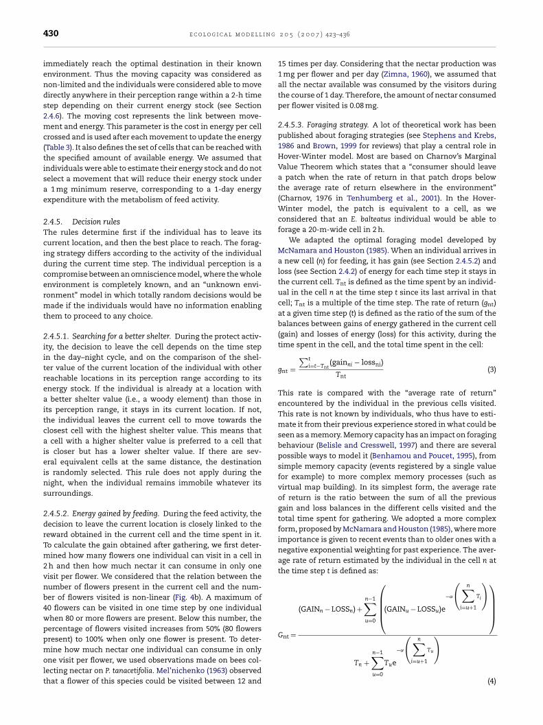
2.4.5.3. Foraging strategy. A lot of theoretical work has beenpublished about foraging strategies (see Stephens and Krebs,1986 and Brown, 1999 for reviews) that play a central role inHover-Winter model. Most are based on Charnov’s MarginalValue Theorem which states that a “consumer should leavea patch when the rate of return in that patch drops belowthe average rate of return elsewhere in the environment”(Charnov, 1976 in Tenhumberg et al., 2001). In the Hover-Winter model, the patch is equivalent to a cell, as weconsidered that an E. balteatus individual would be able toforage a 20-m-wide cell in 2 h.

We adapted the optimal foraging model developed byMcNamara and Houston (1985). When an individual arrives ina new cell (n) for feeding, it has gain (see Section 2.4.5.2) andloss (see Section 2.4.2) of energy for each time step it stays inthe current cell. Tnt is defined as the time spent by an individ-ual in the cell n at the time step t since its last arrival in thatcell; Tnt is a multiple of the time step. The rate of return (gnt)at a given time step (t) is defined as the ratio of the sum of thebalances between gains of energy gathered in the current cell(gain) and losses of energy (loss) for this activity, during thetime spent in the cell, and the total time spent in the cell:

gnt =∑t

i=t−Tnt(gainni − lossni)

Tnt(3)

This rate is compared with the “average rate of return”encountered by the individual in the previous cells visited.This rate is not known by individuals, who thus have to esti-mate it from their previous experience stored in what could beseen as a memory. Memory capacity has an impact on foragingbehaviour (Belisle and Cresswell, 1997) and there are severalpossible ways to model it (Benhamou and Poucet, 1995), fromsimple memory capacity (events registered by a single valuefor example) to more complex memory processes (such asvirtual map building). In its simplest form, the average rateof return is the ratio between the sum of all the previousgain and loss balances in the different cells visited and thetotal time spent for gathering. We adopted a more complexform, proposed by McNamara and Houston (1985), where moreimportance is given to recent events than to older ones with anegative exponential weighting for past experience. The aver-age rate of return estimated by the individual in the cell n atthe time step t is defined as:

Gnt =

(GAINn − LOSSn) +n−1∑u=0

⎛⎜⎜⎜⎝(GAINu − LOSSu)e

−˛

(n∑

i=u+1

Ti

)⎞⎟⎟⎟⎠

(n

)

Tn +

n−1∑u=0

Tue

−˛

∑i=u+1

Tu

(4)

g 2 0

wows

alflsmaottni

2OietsBi(−met

D

w((Dfi

tfvttwnWpOip

2

Sowgi

e c o l o g i c a l m o d e l l i n

here GAINu and LOSSu are the total amount of gain and lossf energy respectively in the cell u, and � is the exponentialeighting factor, corresponding to the adaptive capacity of the

pecies, fixed in the model to 0.05.If the rate of return in the current cell is lower than the

verage rate of return, i.e., gnt < Gnt, then the individual willeave its cell to the closest one with the highest number ofowers in its perception range. If two or more cells have theame high number of flowers at the same distance, then theodel chooses randomly. It should be stressed that the model

ssumes that the individuals are able to estimate the numberf flowers of the surrounding cells, but not their Nectar quan-ity, which can vary greatly depending on previous foraging inhe cells. This implies that the ability to identify the highestumber of flowers does not necessarily imply the highest gain

n the future.

.4.6. Death probabilitynly two reasons for death can intervene at the end of the

nsect time step. The first is loss of energy: if the individualnergy stock falls below 0 (due to its activity and movement)hen its death probability is 1. The second reason is expo-ure to low temperatures. We used data measured by Hart andale (1997) who observed that low temperatures had a strong

mpact on E. balteatus individuals: a temperature of −14 ◦CTD90) led to a mortality of 90% of the individuals, whereas10 ◦C (TD50) and −6 ◦C (TD10) corresponded respectively to aortality of 50% and 10% of the individuals, whatever their

nergy stock. We calibrated a logistic function (5) passinghrough these experimental points (Fig. 4c):

P = 1

(1 + e−b(FT−TD50)/(TD90−TD10))(5)

here DP is the death probability; FT the felt temperaturesee below), TD50 the temperature value at which DP = 0.550%) and DTD80 the difference between temperature at whichP = 0.1 (10%), temperature at which DP = 0.9 (90%), and b is thetting constant coefficient (value: 2 Ln(9) = 4.3944).

The effect of protect activity was translated as a modula-ion of death probability. Death probability is calculated usingelt temperature, which is given by combining the shelteralue of the cell where the individual is currently located andhe Local temperature in this cell. Where the shelter value = 2,he felt temperature has a value of 0 ◦C for the individualsho perform the protect activity when local temperature isegative, and so the death probability in the cell is lowered.here shelter value = 1, the felt temperature is the local tem-

erature increased by one degree when the latter is negative.therwise, when local temperature is positive or when the

ndividual is not performing the protect activity, the felt tem-erature equals the local temperature.

.5. Model outputs

everal outputs can be displayed both during and at the end

f the simulation. The main output is the survival rate (SR),hich represents the percentage of individuals still alive at a

iven step of the simulation. Other outputs provide insightsnto individual behaviours. The mean residence time (MRT)

5 ( 2 0 0 7 ) 423–436 431

is the mean number of time steps spent at a given location,the mean number of visits per land cover type (MNV) repre-sents the mean number of arrivals in each land cover typeduring the course of the simulation, and the mean number oftimes (MNT) is the number of surviving individuals perform-ing each activity (protect or feed). The model calculates alsothe mean moving length (MML), which represents the averagedistance of one move, and the death causal (DC) that informsabout the reason for death: loss of energy or low tempera-ture. In this paper, we only give the output values at the endof the simulation (1080th time step, at the end of the 90 dayssimulation).

2.6. Analyses

The Hover-Winter model was developed using the CORMAS(COmmon-pool Resource and multi-agents system) software(http://cormas.cirad.fr). CORMAS is a multi-agent platformoriginally dedicated to the renewable resources management(Bousquet et al., 1998). It is based on the VisualWorks pro-gramming environment software using the Smalltalk objectoriented language (Visual Works 7.3, Cincom Softwares).

Sensitivity analyses provide results about the influence ofthe uncertainty in defining parameters values. If a small vari-ation in the value of a given parameter induced a significantvariation of the outputs from the model, then it indicated thata stronger effort should be put on a better and more accuratemeasure or estimation of this parameter. Sensitivity analy-ses were performed for six parameters selected for their apriori importance in the model and for the lack of accuracyin their estimations: perception range (PR), moving cost (MC),maximum energy stock (ES), feed activity probability (FAP),death probability (DP) and protect energy cost (PEC). For com-plex parameters defined as a curve of probability (feed activityprobability and death probability), simple sensitivity analyseswere difficult because several characteristics of the parame-ter could have been modified to study it. For the feed activityprobability parameter, we chose to keep the same curve shapeand to use several temperature values defining the 95% feedactivity probability (TFAP95), the other parameters (TFAP50and TFAP5) being deduced from this value as a function ofthe shape of the curve (Fig. 4a). The same method was appliedfor death probability where we also used the same curve pat-tern (Fig. 4c). For each parameter, different ranges of valueswere set for each parameter (including extreme values), all theothers being held constant. The consequences were observedfor the variations of survival rate with 75 repetitions for eachvalue. A set of 200 simulations was run with the referenceparameter values selected for the model (Table 3), and theoutputs were analyzed from an ecological point of view. Themodel was applied on a set of data obtained from a 670 halandscape located in a hilly region of Southwestern Francewhere E. balteatus females are known to overwinter. The spa-tial grid was created from a satellite SPOT image (Fig. 1). Thetemperature data for this area were measured in a north edge

of the landscape from the 20 December 2003 at 2 a.m. to the 19March 2004 at midnight. The temperature ranged from −5.8 to22.5 ◦C, with a mean value of 5.4 ◦C. 2000 individuals were setat the beginnings of the simulations.

i n g

432 e c o l o g i c a l m o d e l l

3. Results

3.1. Sensitivity analysis

Perception range had a negative effect on the survival rate(Fig. 5a), with a mean survival rate of 7% for the smallest per-ception range (five cells) to 4.6% for the largest range (20 cells).The selected value (10 cells) was in an intermediate position inthis range and did present a particular variability. The uncer-tainty of the perception range parameter did not seem to havean influence on the variability of the model output. Extremevalue of moving cost (MC = 7 units of energy per cell crossed),corresponding to almost impossible movement, produced thelowest mean survival rates (4%) (Fig. 5b) and the lowest value(MC = 0.02 units of energy per cell crossed), selected for themodel, corresponded to the highest survival rates, with amean of 5.25%. The uncertainty of this parameter seemed tohave low absolute influence on the output of the model since avariation from 0.02 to 7 units induced a variation of the outputsof only 1.25%, but its relative influence should be consideredsince this variation is 24% of the lowest mean survival rate.Survival rate was positively correlated with the maximum ofenergy stock (Fig. 5c). The selected value (7 mg) did not presenta particular variability of the survival rate. The uncertainty oftemperature of 90% death probability value (TDP90) had con-siderable consequences for the survival rate (Fig. 5f). Withina range of a few degrees, the survival rate increased from 0%(TDP90 = −6 ◦C) to more than 20% (TDP90 = −22 ◦C). A reduc-tion of only 2 ◦C of this parameter resulted in the survival oftwice the number of individuals. We observed that the tem-perature of 95% feed activity probability (TFAP95) had complexconsequences for the survival rate (Fig. 5e): low and high val-ues induced the lowest survival rates whereas intermediatevalues, where was the selected value (13 ◦C), corresponded tothe highest rates. The protect energy cost uncertainty mod-ified the survival rate of the model. Higher value than whathad been selected (0.02 mg) lead to lower survival rates, butthese values are not realistic since our selected value wasalready over-estimated comparatively with existing data. Forlower values, the survival rate was higher but seemed to reacha maximum for small protect energy cost values (0.0008, i.e.,1/100 of the feed energy cost).

3.2. Simulation runs

Starting with 2000 individuals and with the parameter val-ues of Table 3, the survival rate (SR) decreased rapidly in thebeginning of the run and slowly at the end. The mean sur-vival rate was 5.35% (minimum: 1.25%; maximum: 12.10%,standard error: 0.20) at the end of the simulation. The meanresidence time (MRT) in one cell was 5.23 time steps (S.E.: 0.09),corresponding to 10 h. The mean moving length (MML) was4.49 cells (S.E.: 0.02), corresponding to 90 m. The mean num-ber of times output (MNT) for each activity showed that thesurviving individuals spent more time performing the protect

activity (mean number of 908 time steps; S.E.: 2.65) than thefeed activity (mean number of 172 time steps; S.E.: 2.65). Thedeath causal output (DC) showed that death was mainly due tothe effect of low temperatures. Indeed, from the 2000 starting

2 0 5 ( 2 0 0 7 ) 423–436

individuals, a mean of 1122 (S.E.: 10.60) died from cold eventswhereas a mean of 772 (S.E.: 6.98) individuals died from energyloss. During the simulations, the mean number of visits output(MNV) showed that the survivors almost exclusively visitedthe South edge and Meadow land covers with means of 24.5and 30 visits, respectively (Fig. 6). Crop fields and forest centreswere never visited. In some simulations, the survivors visitedNorth edge a few times at the beginning of the winter beforefinding a suitable South edge (overall mean: 4 visits).

4. Discussion

4.1. Hover-Winter model quality

The main objective of the Hover-Winter model was to translatein a spatially explicit model, field data and both bibliograph-ical and expert knowledge, to be able to simulate realisticpopulation dynamics. That objective is reached and Hover-Winter is the first and the most comprehensive individualbased model for E. balteatus. In multi-agent modelling, theease of compiling and combining multiple sets of informationmay produce overcomplicated models which may be very dif-ficult to validate (Conroy et al., 1995; Bousquet and Le Page,2004). Although many parameters were taken into accountin the Hover-Winter model, its overall behaviour was quitestable and outputs never exhibited inconsistent results withthe biological and ecological knowledge about E. balteatus.Hover-Winter has moreover been presented at an interna-tional symposium to several syrphidologists (Arrignon et al.,2005) who regarded its main results as being realistic and eco-logically founded. As an indication of a global and qualitativevalidity, Hover-Winter model reflected qualitatively the samedistribution pattern observed by Sarthou et al. (2005) in south-western France. Surviving individuals, in model outputs andfield data, almost only visited south edges rather than northedges or forest centres. The high visit rate in Meadows exhib-ited by the model is also consistent with field observations.

More quantitative validations are needed but they arelimited by the difficulties to measure, with capture-marking-recapture methods for example, the actual population densityin the landscape that may be very low and unevenly dis-tributed. However, the hypotheses that are derived from theHover-Winter model outputs, based on rates comparisonsand qualitative aspects, could help designing particular sam-pling schemes adapted to these difficulties. Further importantimprovements could be obtained with a more detailed designof the temperature and food sub-models that are rather roughin the current version of Hover-Winter. For example temper-ature and nectar production could be linked and the effect ofboth air humidity and wind could be added to weather condi-tions.

Sensitivity analyses are also a key step towards a qualita-tive validation of the model (Rykiel, 1996). For perception range(MacLeod, 1999), feed activity temperature (Gilbert, 1985) ordeath probability (Hart and Bale, 1997), reliable information

was available in the literature. For moving cost parameter,information was lacking. As this parameter was only roughlyqualitatively estimated, classical experiments using Turchin’sdesign with mark-recapture techniques (Turchin, 1998) could

e c o l o g i c a l m o d e l l i n g 2 0 5 ( 2 0 0 7 ) 423–436 433

Fig. 5 – Sensitivity of the survival rate output to parameters uncertainty. Sensitivity analyses were used to estimate how theuncertainty of the model parameters influences the variability of its outputs. A range of values was tested for eachparameter, the other being held constant, in a set of 75 simulation runs for each value, with the same model inputs (see textfor details and Table 3 for parameter definitions). The figures present the effects on the survival rate of the perception range(a), the moving cost (b), the maximum energy stock (c), the protect energy cost (d), the temperature of 95% feed activityp andS

btdHs

robability (e) and the temperature of 90% death probability.E.: standard error and S.D.: standard deviation.

e conducted to assess it more accurately. For the parameters

ested and presented in this paper, the temperature of 90%eath probability, fixed in our model at −14 ◦C according toart and Bale (1997) data, was the only one that induced a

ignificant variability in the rate of survival output, for small

(f) the abscisses are discontinued where X-axis is missing.

variations. A small error of ±2 ◦C in the estimation of this

parameter would have disproportionate consequences on therate of survival estimated with temperature data from south-western France. The value selected for protect energy cost washigher than what was available for other species in the liter-

i n g

434 e c o l o g i c a l m o d e l l

ature. The winter conditions may induce a higher energy losswhen protecting, and the 2-h time step means that the individ-uals may perform other short time activities during the pro-tecting period, and thus may lose more energy than what theymay lose when they are strictly resting. The selected valueinduces a lower rate of survival than what could be expectedwith lower protect energy costs; however, even for very lowvalues, the rate of survival did not varies a lot (25% increase ofrate of survival for a protect energy cost divided by 100).

Sensitivity results may be interpreted also from an evo-lution perspective and used as a way to assess what is theinfluence of biological characteristics of the modelled specieson its fitness and ability to overwinter. As an example, the sen-sitivity results showed that the potential fitness improvementobtained via a movement is mostly linked with the equilib-rium between energy stock, moving cost and the gain obtainedafter the movement. The increase in the survival rate is mainlydue to the fact that the individual is able to survive muchlonger in the same place without moving, as the maximalenergy stock increases. When moving cost is high but notextreme, the individuals are able to reach a good site earlyin the simulation and then to survive there for the rest of thesimulation.

4.2. Ecological interpretation of Hover-Winter outputs

In the outputs of the simulations realized with the southwest-

ern France landscape and temperature series, 5/6th of the timewas spent on the protect activity, and around half this timeduring daytime, which is consistent with the fact that the win-ter temperature conditions do rarely allow feeding activities.

Fig. 6 – Distribution of the number of visits in land coverclasses during the simulations: the visits of the 2000 initialindividuals in each land cover classes during the 1080 timesteps of the 200 simulations of reference with the sameinput data (see text for details) were recorded. Thedistribution of the mean number of visits per landcoverclass shows that most individuals that survived visitedMeadows and South edges. Some insects that survived alsovisited North edges early in winter before finding a suitableSouth edge. Fields and forest centres were almost nevervisited. S.E.: standard error and S.D.: standard deviation.

2 0 5 ( 2 0 0 7 ) 423–436

The fact that most of the individuals died from low temper-ature showed that the ability to reach a shelter is of primeimportance for survival. 772 individuals among 2000 died dueto loss of energy, demonstrating how important the ability toperform the feed activity is for survival. The surviving indi-viduals mostly visited south edges and meadows. The meanmoving length (90 m) was not as great as expected comparedto the values for perception range (200 m).

From these results we deduce that the surviving individualsare mostly those located in a close “South edge-Meadow” cou-ple. When these individuals find this favourable combination,they are able to survive the whole winter as it combines highflower availability in the meadow and high shelter value in theedge, with sufficient days with high temperatures (South edge)for the individual to be active enough to reach the flowersin the neighbourhood. The relatively short distance betweenthese two landscape elements minimizes the energy spentand thus maximizes the survival rate. This leads us to assumethat E. balteatus follows a landscape complementation strat-egy (Dunning et al., 1992) during the winter part of its lifecycle. Meadows and edges would represent complementaryfactors (respectively energy and shelter) for the individuals,although North edge populations would not be viable due tolow temperatures.

The individual behaviours observed in the model areclosely linked to the decision to leave or not their location at agiven time step and that could explain emerging properties atthe population scale (Johnson et al., 1992; Russell et al., 2003;Breckling et al., 2005). Since the nectar resource decreases inthe current cell if the individual keeps on gathering it, the for-aging model adapted from McNamara and Houston’s modelforces the individual to find another suitable location that mayor not provide a higher rate of gain. However, since individualsare seldom active in winter due to low temperatures, there isvery low competition between individuals and the flowers inthe cell have therefore time to restore their nectar quantity. Inthis way, when an individual is feeding, the nectar quantity ofits current location is frequently maximal and the gnt thus donot frequently drop below Gnt. This could explain why someindividuals stay in the same location throughout the simula-tion. When it is not the case, the new location could be fartherfrom a potential shelter, and this decision may not be the mostappropriate to improve individual fitness if a low temperatureperiod occurs, preventing other movements towards a shelter.This balance between the probability to get a higher gain andthe probability to be in a more vulnerable situation introducesa complex system in the model that can be studied throughsets of repeated simulations in contrasted conditions accord-ing to the spatial distribution of food resources and shelters.

The complex effect of temperature on survival raises thefollowing question: “what is a good winter for E. balteatus”?If very cold temperatures have a negative impact on survival,warm temperatures are necessary to allow the insects to flyand feed. Thus, a climate with frequent periods with hightemperature, in sunny conditions for example, may be morefavourable than a more even climate with a higher mean tem-

perature but less numerous high temperature days. Very coldwinters with low temperatures at night may not be disastrousif relative high temperatures occur during the day in parts oflandscape that are close to flower resources.

g 2 0

5

TocgdspaleatusBsbbaem

A

Wfiuctolabgp

r

A

A

A

A

A

e c o l o g i c a l m o d e l l i n

. Conclusion

he open structure of multi-agent systems, where differentbjects with different properties can be combined in a set ofomplex and evolving relationships, is appealing for ecolo-ists who frequently observe that most ecological processeso not easily fit the frame of equation-based models. Thistructure is able to integrate in the same model very differentieces of knowledge. In our study, we were able to take intoccount field data and most of the knowledge available in theiterature and from experts of E. balteatus. This approach alsonabled us to identify crucial knowledge gaps. Using observednd published data, theoretical models and expert knowledge,he Hover-Winter model enabled a study of the role of individ-al behaviour in the dynamics of a population at the landscapecale (Turchin, 1991; Roese et al., 1991; South, 1999; Bowne andowers, 2004). However, these processes remain difficult totudy, as they combine biological and ethological data. Agent-ased models are useful tools for modelling such complexehaviours in a spatially explicit way as they produce a hugemount of output data that can be analyzed to generate newcological hypothesis to explain the patterns observed thatay be tested in the field.

cknowledgements

e thank Sylvie Ladet, Alexandre Leray and Bernard Bouyjouor their contribution to this study, by providing field and datamplementation help. We also thank Pierre Margerie for hisseful comments on earlier versions of the manuscript, Fran-is Gilbert, Francois Bousquet and Jean-Louis Hemptinne forheir valuable and insightful advices during the PhD defencef Florent Arrignon, Daphne Goodfellow for revising English

anguage. The paper was written while the first author heldgrant from the French Ministry of Research. This study has

een funded by the French Ministry of Research (PSDR pro-ram) and by the Midi-Pyrenees Regional Council (CCRRDTrogram).

e f e r e n c e s

ltieri, M.A., Nicholls, C.I., 1999. Biodiversity, ecosystemsfunction and insect pest management in agricultural systems.In: Collins, W.W., Qualset, C.O. (Eds.), Biodiversity inAgroecosystems. CRC Press, New York, pp. 69–84.

rrignon, F., 2006. HOVER-WINTER: un modele multi-agent poursimuler la dynamique hivernale d’un insecte auxiliaire descultures (Episyrphus balteatus, Diptera: Syrphidae) dans unpaysage heterogene. Institut National Polytechnique deToulouse. PhD Thesis. 220 pp.

rrignon, F., Sarthou, J.P., Deconchat, M., Monteil, C., 2005. Whatshould we know about Episyrphus balteatus to improve themodelling of its individual overwintering survival? In:Proceedings of the Third International Symposium on theSyrphidae, Leiden, The Netherlands, September 2–5.

ubert, J., Goeldlin, P., Lyon, J.P., 1969. Essais de marquage et dereprise d’insectes migrateurs en automne 1968. Bulletin de laSociete Entomologique Suisse 42, 140–166.

ubert, J., Aubert, J.J., Goeldlin, P., 1976. Douze ans de capturessystematiques de Syrphides (Dipteres) au col de Bretolet

5 ( 2 0 0 7 ) 423–436 435

(Alpes valaisannes). Mitteilungen der SchweizerischenEntomologischen Gesellschaft 49, 115–142.

Beane, K.A., Bugg, R.L., 1998. Natural and artificial shelter toenhance arthropod biological control agents. In: Pickett, C.H.,Bugg, R.L. (Eds.), Enhancing Biological Control. University ofCalifornia Press, Los Angeles, pp. 239–253.

Belisle, C., Cresswell, J., 1997. The effects of a limited memorycapacity on foraging behavior. Theor. Populat. Biol. 52,78–90.

Benhamou, S., Poucet, B., 1995. A comparative analysis of spatialmemory processes. Behav. Process. 35, 113–126.

Berec, L., 2002. Techniques of spatially explicit individual-basedmodels: construction, simulation, and mean-field analysis.Ecol. Model. 150, 55–81.

Bianchi, F., van der Werf, W., 2004. Model evaluation of thefunction of prey in non-crop habitats for biological control byladybeetles in agricultural landscapes. Ecol. Model. 171,177–193.

Booch, G., Rumbaugh, J., Jacobson, I., 1999. The Unified ModelingLanguage, User Guide. Addison-Wesley, Reading, MA, 482 pp.

Bousquet, F., Bakam, I., Proton, H., Le Page, C., 1998. Cormas:common-pool resources and multi-agent systems. Lect. NotesArtif. Intel. 1416, 826–838.

Bousquet, F., Le Page, C., 2004. Multi-agent simulations andecosystem management: a review. Ecol. Model. 176, 313–332.

Bowne, D.R., Bowers, M.A., 2004. Interpatch movements inspatially structured populations: a literature review. Landsc.Ecol. 19, 1–20.

Breckling, B., Muller, F., Reuter, H., Holker, F., Franzle, O., 2005.Emergent properties in individual-based ecologicalmodels—introducing case studies in an ecosystem researchcontext. Ecol. Model. 186, 376–388.

Brown, J.S., 1999. Foraging ecology of animals in response toheterogeneous environments. In: Hutchings, M., John, E.A.,Stewart, A.J., Webb, N.R. (Eds.), Ecological Consequences ofEnvironmental Heterogeneity. Blackwell Editor, London, pp.181–214.

Conroy, M., Cohen, Y., James, F., Matsinos, Y., Maurer, B., 1995.Parameter estimation, reliability, and model improvement forspatially explicit models of animal populations. Ecol. Appl. 5,17–19.

Cowgill, S.E., Wratten, S.D., Sotherton, N.W., 1993. The selectiveuse of floral resources by the hoverfly Episyrphus balteatus(Diptera: Syrphidae) on farmland. Ann. Appl. Biol. 122,223–231.

De Angelis, D., Gross, L.J., 1992. Individual-Based Models andApproaches in Ecology: Populations, Communities andEcosystems. Chapman and Hall, New York.

Dunning, J., Danielson, B., Pulliam, H., 1992. Ecological processesthat affect populations in complex landscapes. Oikos 65,169–175.

Ferber, J., 1995. Systemes Multi-Agents: Vers une IntelligenceCollective. Intereditions, Paris, 522 pp.

Ferber, J., 1999. Multi-Agent Systems: An Introduction toDistributed Artificial Intelligence. Addison-Wesley, Reading,MA, 528 pp.

Gilbert, F.S., 1985. Diurnal activity patterns in hoverflies (Diptera,Syrphidae). Ecol. Entomol. 10, 385–392.

Grimm, V., 1999. Ten years of individual-based modelling inecology: what have we learned and what could we learn inthe future? Ecol. Model. 115, 129–148.

Gurr, G.M., Wratten, S.D., Altieri, M.A. (Eds.), 2004. EcologicalEngineering for Pest Management—Advances in HabitatManipulation for Arthropods. CSIRO Publishing, Collingwood,

CABI Publishing, Oxon, 256 pp.

Hart, A.J., Bale, J.S., 1997. Cold tolerance of the aphid predatorEpisyrphus balteatus (DeGeer) (Diptera, Syrphidae). Physiol.Entomol. 22, 332–338.

i n g

436 e c o l o g i c a l m o d e l l

Haslett, J.R., 1989. Interpreting patterns of resource utilization:randomness and selectivity in pollen feeding by adulthoverflies. Oecologia 78, 433–442.

Heinrich, B., 1979. Bumblebee Economics. Harvard UniverityPress, Cambridge, MA, 245 pp.

Heinrich, B., 1981. Insect Thermoregulation. John Wiley & Sons,New York, 329 pp.

Huston, M., De Angelis, D., Pott, W., 1988. New computer modelsunify ecological theory. Bioscience 38, 682–691.

Johnson, A.R., Wiens, J.A., Milne, B.T., Crist, T.O., 1992. Animalmovements and population dynamics in heterogeneouslandscapes. Landsc. Ecol. 7, 63–75.

Jopp, F., Reuter, H., 2005. Dispersal of carabid beetles–emergenceof distribution patterns. Ecol. Model. 186, 389–405.

Lewis, T., 1965. The effects of an artificial wind break on the aerialdistribution of flying insects. Ann. Appl. Biol. 55, 503–512.

Lorek, H., Sonnenschein, M., 1998. Object-oriented support formodelling and simulation of individual-oriented ecologicalmodels. Ecol. Model. 108, 77–96.

Lyon, J.P., 1967. Deplacements et migrations chez les Syrphidae.Annales des Epiphyties 18, 117–118.

MacLeod, L., 1999. Attraction and retention of Episyrphus balteatusDeGeer (Diptera: Syrphidae) at an arable field margin with richand poor floral resources. Agric. Ecosyst. Environ. 73, 237–244.

McNamara, J.M., Houston, A.I., 1985. Optimal foraging andlearning. J. Theor. Biol. 117, 231–249.

Mel’nichenko, A.N., 1963. Bees themselves increase the nectarproductivity of flowers. Pchelovodstvo 40, 32–35.

Ngamo-Tinkeu, L.S., 1998. Atouts biologiques, ecologiques etmorphologiques precisant l’utilite de Episyrphus balteatus (deGeer, 1776) (Diptera: Syrphidae) dans la lutte biologique.Universite Catholique de Louvain. PhD Thesis. 210 pp.

Poehling, H.-M., 1988. Auftreten von Syrphiden- undCoccinellidenlarven in Winterweizen von 1984-1987 inRelation zur Abundanz von Getreideblattlausen. Mitteilungender Deutschen Gesellschaft fur allgemeine und angewanteEntomologie 6, 248–254.

Roese, J., Risenhoover, K., Folse, L., 1991. Habitat heterogeneity

and foraging efficiency: an individual-based model. Ecol.Model. 57, 133–143.

Russell, R., Swihart, R., Feng, Z., 2003. Population consequencesof movement decisions in a patchy landscape. Oikos 103,142–152.

2 0 5 ( 2 0 0 7 ) 423–436

Rykiel, J., 1996. Testing ecological models: the meaning ofvalidation. Ecol. Model. 90, 229–244.

Sarthou, J.P., 1996. Contribution a l’etude systematique,biogeographique et agroecocenotique des Syrphidae (Insecta,Diptera) du Sud-Ouest de la France. Institut NationalPolytechnique Toulouse. PhD Thesis. 251 pp.

Sarthou, J.P., Ouin, A., Arrignon, F., Barreau, G., Bouyjou, B., 2005.Landscape parameters explain the distribution andabundance of Episyrphus balteatus (Diptera: Syrphidae). Euro. J.Entomol. 102, 539–545.

Schneider, F., 1948. Beitrag zur Kenntnis derGenerationsverhaltnisse und Diapause rauberischerSchwebfliegen (Syrphidae, Dipt.). Mitteilungen derSchweizerischen Entomologischen Gesellschaft 21, 249–285.

South, A., 1999. Extrapolating from individual movementbehaviour to population spacing patterns in a rangingmammal. Ecol. Model. 117, 343–360.

Stephens, D.W., Krebs, J.R., 1986. Foraging Theory. PrincetonUniversity Press, Princeton, NJ, 247 pp.

Tenhumberg, B., Poehling, H.M., 1995. Syrphids as naturalenemies of cereal aphids in Germany: aspects of their biologyand efficacy in different years and regions. Agric. Ecosyst.Environ. 52, 39–43.

Tenhumberg, B., Keller, M., Possingham, H., Tyre, A., 2001.Optimal patch-leaving behaviour: a case study using theparasitoid Cotesia rubecula. J. Anim. Ecol. 70, 683–691.

Topping, C.J., Hansen, T.S., Jensen, T.S., Jepsen, J.U., Nikolajsen, F.,Odderskaer, P., 2003. ALMaSS, an agent-based model foranimals in temperate European landscapes. Ecol. Model. 167,65–82.

Turchin, P., 1991. Translating foraging movements inheterogeneous environments into the spatial distribution offoragers. Ecology 72, 1253–1266.

Turchin, P., 1998. Quantitative Analysis of Movement: Measuringand Modeling Population Redistribution in Animals andPlants. Sinauer Associates, Sunderland, MA, 396 pp.

Wratten, S.D., van Emden, H.F., Thomas, M.B., 1998. Within-fieldand border refugia for the enhancement of natural enemies.

In: Pickett, C.H., Bugg, R.L. (Eds.), Enhancing Biological Control.University of California Press, Los Angeles, pp. 375–403.

Zimna, J., 1960. Etudes comparatives sur la secretion nectariferede quatre especes de phacelia. Pszczelnicze Zeszyty Naukowe4, 167–174.