modelling the effect of food depletion on scallop growth in sungo bay (china

Original article

Modelling the effect of food depletionon scallop growth in Sungo Bay (China)

Cédric Bachera,*, Jon Grantb, Anthony J.S. Hawkinsc, Jianguang Fangd,Mingyuan Zhue, Mélanie Besnarda

a Ifremer, Crema, BP 5, 17137 L’Houmeau, Franceb Department of Oceanography, Dalhousie University, 1355 Oxford Street, Halifax, NS, Canada B3H 4J1

c Plymouth Marine Laboratory, Prospect Place, Plymouth PL1 3DH, UKd Chinese Academy of Fishery Sciences, 106 Nanjing Road, 266071 Qingdao, People’s Republic of China

e SOA-FIO, Xianxialing Road, Hi-Tech Industrial Park, 266061 Qingdao, People’s Republic of China

Received 29 April 2002; accepted 10 January 2003

Abstract

Sungo Bay (China) has a mean depth of 10 m, a total area of 140 km2 and is occupied by several types of aquaculture, whilst opening to theocean. The production of scallops (Chlamys farreri) cultured on long lines is estimated to exceed 50 000 tonnes (total weight) per year.Selection of sites for scallop growth and determination of suitable rearing densities have become important issues. In this study, we focused onthe local scale (e.g. 1000 m) where rearing density, food concentration and hydrodynamics interact. We have developed a depletion modelcoupling a detailed model ofC. farreri feeding and growth and a one-dimensional horizontal transport equation. The model was applied toassess the effect of some environmental parameters (e.g. food availability, temperature, hydrodynamism) and spatial variability on growth, andto assess the effect of density according to a wide range of hydrodynamical and environmental conditions. In the simulations, foodconcentrations always enabled a substantial weight increase with a final weight above 1.5 g dry weight. Compared to a reference situationwithout depletion, a density of 50 ind m–3 decreased growth between 0% and 100%, depending on current velocity when maximum currentvelocity was below 20 cm s–1. The mean ratio between food available inside and outside the cultivated area (depletion factor) varied with thepercentage of variation in scallop growth that was due to density. Our model suggests that scallop growth was correlated with maximumcurrent velocity for a given density and current velocity below 20 cm s–1. The model was integrated within a Geographical Information System(GIS) to assist in making decisions related to appropriate scallop densities suitable for aquaculture at different locations throughout the bay.Concepts (depletion), methods (coupling hydrodynamics and growth models), and the underlying framework (GIS) are all generic, and can beapplied to different sites and ecosystems where local interactions must be taken into account.

© 2003 Éditions scientifiques et médicales Elsevier SAS and Ifremer/IRD/Inra/Cemagref. All rights reserved.

Résumé

Modélisation de l’effet de la diminution de nourriture sur la croissance du pétoncle dans la baie de Sungo (Chine). La baie deSungo (Chine) est une baie largement ouverte sur l’océan, qui occupe une surface de 140 km2 pour une profondeur moyenne de 10 m et dontune grande partie est consacrée à l’aquaculture. La production annuelle de pétoncles (Chlamys farreri) dépasse ainsi les 50 000 tonnes (poidstotal). La sélection de sites et la définition de densité d’élevage favorables à la croissance sont devenues un enjeu important. Nous avonsdéveloppé un modèle mathématique prenant en compte les interactions entre densité d’élevage, concentration de nourriture et hydrodyna-misme à un niveau local, défini par une distance typique de 1000 m, afin de prédire la diminution de nourriture liée à la consommation par lespétoncles (appelée par la suite « déplétion ») et son effet sur la croissance. Ce modèle s’appuie d’une part sur des équations détaillant lanutrition et la croissance du pétoncle et d’autre part sur un modèle de transport horizontal unidimensionnel. Il permet d’évaluer l’effet desconditions environnementales (nourriture, température, hydrodynamisme) et de leur variabilité spatiale sur la croissance et de tester l’influencede la densité d’élevage pour ces différentes conditions. Nous avons comparé une situation sans déplétion (où la croissance est maximale) à unesituation avec une densité d’élevage de 50 ind par m3. Le modèle indique des diminutions de croissance entre 0 et 100 % en fonction de lavitesse du courant tant que la vitesse maximale reste en dessous de 20 cm s–1. Cette variation de croissance annuelle peut être mise en relation

* Corresponding author.E-mail address: [email protected] (C. Bacher).

Aquat. Living Resour. 16 (2003) 10–24

www.elsevier.com/locate/aquliv

© 2003 Éditions scientifiques et médicales Elsevier SAS and Ifremer/IRD/Inra/Cemagref. All rights reserved.DOI: 1 0 . 1 0 1 6 / S 0 9 9 0 - 7 4 4 0 ( 0 3 ) 0 0 0 0 3 - 2

avec le rapport entre la concentration moyenne de nourriture à l’ intérieur et à l’extérieur du domaine cultivé, qui est un indice de déplétionreflétant principalement l’effet de la vitesse du courant. Le modèle a été intégré àun Système d’ Informations Géographiques (SIG) ce quipermet de simuler et cartographier rapidement et automatiquement la croissance annuelle et de fournir ainsi des recommandations sur ladensitéd’élevage appropriée. Le concept de déplétion, le couplage d’un modèle de croissance et d’un modèle hydrodynamique et l’utilisationd’un SIG sont transposables à d’autres systèmes comparables dans lesquels les interactions locales doivent être considérées.

© 2003 Éditions scientifiques et médicales Elsevier SAS and Ifremer/IRD/Inra/Cemagref. Tous droits réservés.

Keywords: Energy budget; Rearing density; Transport equation; Chlamys farreri

1. Introduction

The development of shellfish aquaculture raises questionsregarding its sustainability defined via the carrying capacityconcept, i.e. the maximum production achievable in a givenecosystem given the biological constraints and characteris-tics of the aquaculture activity. Assessment of the maximumyield is relevant if one considers that little was known untilrecently on regarding the capacity of ecosystems to supportaquaculture activity apart from some empirical knowledge orsuccessful/unsuccessful trials to adapt different species incoastal areas. Since shellfish production is an important com-ponent of the fisheries resources of coastal communities,carrying capacity assessment has become a major focus ofscientific studies facilitating coastal zone management.

These topics are of particular importance in China wheretraditional aquaculture has been ongoing for centuries, buthas been undergoing especially rapid growth in the past 10years (Guo et al., 1999). Coastal zone management in Chinahas become a major concern because of the following rea-sons: (i) the impact of human activities on environmental andwater quality, and (ii) the need for optimization of aquacul-ture strategy (Fang et al., 1996). Within this context, a projectwas funded by the European Union to build tools capable ofcharacterizing the carrying capacity and impact of shellfishand kelp aquaculture in two Chinese bays situated in Shan-dong province. Cooperative studies were conducted on thefeeding responses and growth of cultivated species, variationin key environmental parameters in the field, and modellinghydrodynamics, filter-feeder growth and ecosystem dynam-ics.

When addressing carrying capacity assessment, an impor-tant first step is to describe and quantify the relationshipbetween filter-feeders and the environment, considering eco-physiological processes such as food filtration, ingestion,assimilation and metabolic losses (Dame, 1993). Physiologi-cal processes are driven by temperature, food concentration(particulate organic matter (POM), phytoplankton) flow andtotal suspended matter concentration which act on the abilityof the individual to ingest or to reject a fraction of theavailable food as pseudofaeces. Modelling these processesallows prediction of the relationship between individualscope for growth (SFG) and environmental factors. Eco-physiology models have been published recently for Mytilusedulis (Scholten and Smaal, 1998; Grant and Bacher, 1998),Crassostrea virginica (Powell et al., 1992), Crassostrea gi-

gas (Raillard et al., 1993; Barilléet al., 1997; Ren and Ross,2001), pearl oyster Pinctada margaritifera (Pouvreau et al.,2000), Tapes philippinarum (Solidoro et al., 2000), whichcan be used to identify food limitation. A second step is todefine the geographical scale of any food limitation. Carry-ing capacity may be defined at the ecosystem scale whenmajor parts of the bay are occupied by aquaculture (Raillardand Menesguen, 1994; Dowd, 1997; Bacher et al., 1998;Ferreira et al., 1998). Tidal currents and the geographicalposition of filter-feeders may also result in a low percentageof food used by those filter-feeders (Grant, 1996), so thatinvestigations at local scales are relevant when rearing den-sity and/or low currents are suspected to influence growththrough food depletion (Incze et al., 1981; Pilditch et al.,2001; Pouvreau et al., 2000). An understanding of foodlimitation in cultured populations assists managers in defin-ing the suitability of sites for aquaculture (Nath et al., 2000).

This paper is one of a series dealing with carrying capacityassessment in Sungo Bay at different spatial scales. SungoBay is a small bay with a mean depth of 10 m, total area of140 km2, opening to the ocean and occupied by several typesof aquaculture, e.g. kelp (Laminaria laminaria), oysters(Crassostrea gigas) and scallops in lantern nets (Chlamysfarreri) (Fig. 1). It is one of the most intensively culturedbays in China. The current velocity is driven by the tide and isusually <20 cm s–1. Due to low nutrient inputs from rivers,

Fig. 1. Location of Sungo Bay (China).

11C. Bacher et al. / Aquat. Living Resour. 16 (2003) 10–24

primary production originates from the import of organicmatter and nutrients from the sea, including recycling ofnitrogen within the bay. The total production and standingstocks have changed over the past 20 years, including a shiftfrom kelp to shellfish production. However, overexploitationis apparent from reduced shellfish growth and the increasedincidence of disease. Scallops are the dominant cultivatedfilter-feeders, and production is estimated as ~50 000 tonnes(total weight) per year. Selection of sites favourable forscallop growth, and determination of suitable rearing densi-ties have become important issues. We focus here on the localscale where rearing density, food concentration and hydrody-namics interact. The first objective was to assess individualscallop growth by combining a hydrodynamic model to pre-dict current velocity and food delivery (Grant and Bacher,2001) with an ecophysiological model to predict responsiveadjustments in scallop feeding and growth (Fig. 2) (Hawkinset al., 2002), taking into account any food depletion. Thecombined “depletion model” was used to simulate individualgrowth at several sites where food concentration had beenmeasured, determining the sensitivity of annual growth toscallop density. The second objective was to integrate themodel within a Geographical Information System (GIS) toassist in making decisions about the appropriate densitiessuitable for aquaculture at different sites throughout SungoBay.

2. Methodology

2.1. Depletion model

The depletion model is coupling food transport, foodconsumption by the scallop population and scallop growth atthe scale of a cultivated area—e.g. within a domain of a givenlength (typically 1000 m). Since we restricted the computa-tions to local scales, we considered the main direction of thecurrent at a given site. The model is based on a one-

dimensional (1D) equation comparable to Pilditch et al.(2001) and Wildish and Kristmanson (1997) when verticalmixing prevents a vertical gradient of particle concentration:

�C�t + u�C

�x = N ⋅ f� C, w � (1)

where C refers to either phytoplankton, organic or inorganicparticulate matter, u is the current velocity, f(C,w) is theindividual food consumption, N is scallop density, w is scal-lop tissue dry weight (DW), x is the distance along the maincurrent direction. Compared to Pilditch et al. (2001), weneglected dispersion terms, since (i) dispersion coefficientsare difficult to determine, (ii) their major effect is smoothingthe variation inside the domain, and (iii) the numerical inte-gration scheme yields numerical dispersion. Food depletionis related to consumption by animals, which was derivedeither from the ingestion rate or filtration rate. Filtration ratewould indeed modify the particle concentration, but an im-portant fraction of the filtered particles would remain in thewater column as pseudofaeces and would be reused by filter-feeders. On the other hand, it could also be argued that theseparticles would likely sink and therefore would not be avail-able for other animals. This is the reason why we comparedtwo models by calculating depletion due either to filtration oringestion rate. In both the cases forcing functions and themodel of scallop growth were the same (see the followingdescription). When depletion was related to ingestion, foodcontained in the pseudofaeces was reused with the sameefficiency and energy content.

The weight change of the scallop is described by:dw� x, t �

dt = g� C, w, T � (2)

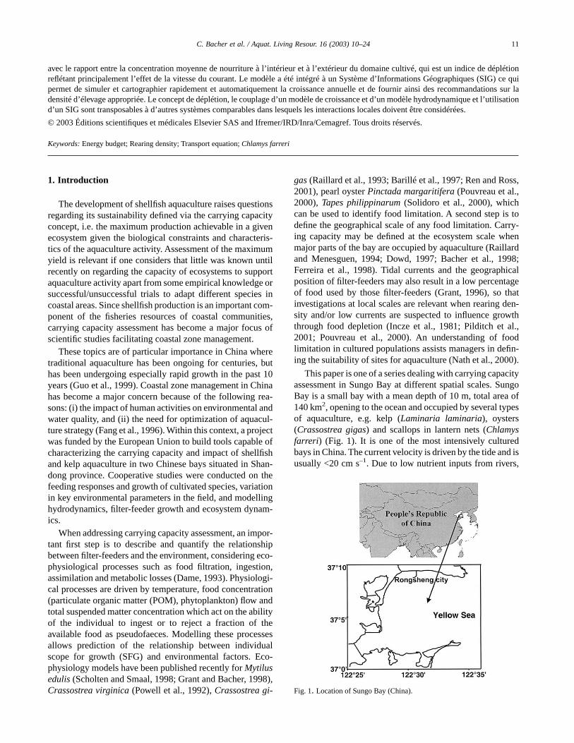
where T is the water temperature and g(C,w,T) is net energybalance established using a model of feeding and growth thathas been developed, calibrated and validated for C. farreri onthe basis of field measurements in Sungo Bay (Hawkins etal., 2002) (refer Table 1 and Fig. 2 for details). In this model,the rates of filtration, ingestion, assimilation and respirationare predicted from the abundances of total particulate matter(TPM), POM and chlorophyll a, including seawater tempera-ture. Net energy balance is determined as the differencebetween rates of assimilation and respiration, and the balanceis allocated between somatic tissue, shell and reproduction.Eqs. (1) and (2) above use these functions from the model ofHawkins et al. (2002) to couple food concentration andscallop growth, such that high scallop densities were ex-pected to result in increased food depletion and diminishedgrowth.

Current velocity was predicted by a hydrodynamic modeldescribed in Grant and Bacher (2001). This model computeswater height and current velocity on an irregular grid of 227nodes all over the bay, which yields more accurate calcula-tions in the area of strong gradients as in the vicinity of thecoastline (Fig. 3a). However, using model outputs at selectednodes for the depletion model requires water mass conserva-tion along the x-axis used in the 1D model. Assuming that thevariation in time of the water height is computed by the 2D

Fig. 2. Conceptual scheme of the scallop feeding and growth model (fromHawkins et al., 2002). Food sources are POM and phytoplankton. Physio-logy functions also depend on temperature and PIM. Filtration, ingestion,pseudofaeces and faeces production are computed for POM, PIM andphytoplankton (see Table 1 for details).

12 C. Bacher et al. / Aquat. Living Resour. 16 (2003) 10–24

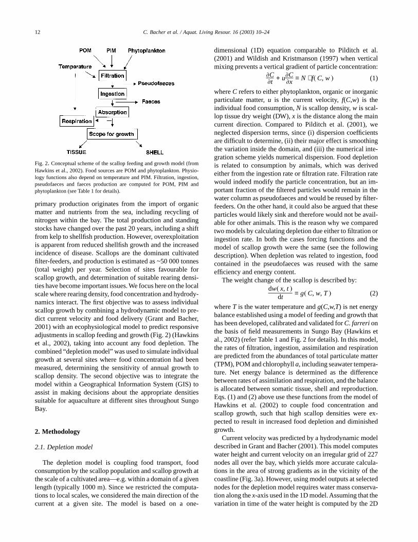
Table 1List of equations for the ecophysiological model of scallop feeding and growth (from Hawkins et al., 2002)

Equations CommentsForcing functionsPHYORG = CHL * chl2phy Phytoplankton (mg l–1)POM Particulate organic matter (mg l–1)TPM Total particulate matter (mg l–1)PIM Particulate inorganic matter (mg l–1)DETORG = POM - PHYORG Detritus (mg l–1)OCS = POM/TPM Food organic contentTEMP Temperature (°C)State variables (initial value)TDW (0.116) Tissue dry weight (g)SDW (0.903) Shell dry weight (g)SEC (265) Shell energy content (J)TEC (2312) Tissue energy content (J)ParametersEDET = 6.1 POM energy content (J mg–1)DW_standard = 1 Standardization weight (g)Allo_feed = 0.62 Allometry coefficient for the ingestionAllo_resp = 0.72 Allometry coefficient for the respirationEnergy_ratio = 0.897 Energy ratio between soft tissue and soft tissue plus shell energytissue2energy = 20 Tissue mass to energy conversion coefficient (J mg–1)shell2energy = 0.294 Shell mass to energy conversion coefficient (J mg–1)chl2phy = 0.1316 Chlorophyll to mass conversion coefficient (mg phyto µg chla–1)Filtration rate (mg d–1)Temp_lim = 2.751 * exp(- 0.00973 * (TEMP - 22.2).^2) Temperature effectallo_ir = (TDW/DW_standard) ** allo_feed Allometry functionFRPHY = exp(2.598 + (5.88 * (log(log(POM) + 1))) + (3.56 * Phytoplankton(log(POM) + 1)) + (0.406 * PHYORG)) * Temp_lim * allo_ir * 24FRDET = (0.542 + 0.586 * DETORG) * Temp_lim * allo_ir * 24 DetritusFRPOM = FRDET + FRPHY POMFRPIM = 19.06 * (1 - exp(- 0.110 * (PIM - 1.87))) * Temp_lim * allo_ir * 24 PIMFRTPM = FRPHY + FRPIM + FRDET TPMPHYCNFPOM = FRPHY/FRPOM Filtrated phytoplankton concentrationRejection rate (mg d–1)RRFRPHYORG = 1.0 – (0.895 * PHYCNFPOM) Phytoplankton enrichment factorRRDET = – 0.00674 + (0.348 * FRDET) DetritusRRPHY = FRPHY * RRFRPHYORG PhytoplanktonRRPIM = – 0.841 + 0.936 * FRPIM PIMRRTPM = RRDET + RRPHY + RRPIM TPMIngestion rate (mg d–1)IRTPM = FRTPM - RRTPM TPMIRDET = FRDET - RRDET DetritusIRPHY = FRPHY - RRPHY PhytoplanktonIRPIM = FRPIM - RRPIM PIMOCI = (IRDET + IRPHY)/IRTPM Ingestion organic contentOIR = IRPHY + IRDET Organic ingestion rateSelection efficiencyDETSEING = (IRDET/IRTPM)/(FRDET/FRTPM) DetritusPHYSEING = (IRPHY/IRTPM)/(FRPHY/FRTPM) PhytoplanktonPIMSEING = (IRPIM/IRTPM)/(FRPIM/FRTPM) PIMAbsorption rate (J d–1)NAEIO = 1.12 – 0.129 * 1/OCI Net absorption efficiencyNEA = (23.5 * IRPHY + EDET * IRDET) * NAEIO Net absorption rateRespiration rate (J d–1)Temp_loss = exp(0.074 * TEMP)/0.33 Temperature effectMaint_heat_loss = 3.55 * 24 * Temp_loss * Maintenance(TDW/DW_standard) ** allo_resp Total_heat_loss = 0.23 * NEA + Maint_heat_loss Total respirationExcretion rate (µg NH 4 d–1)O2N = 10 + 0.05 * NEA Conversion from oxygen to nitrogen


hydrodynamic and is uniform in space at the local scale, wewrote the same mass conservation equation as Roberts et al.(2000):

h ⋅ �u�x + �h

�t = 0 (3)

where h is the water height. The current velocity thereforevaries in space and time.

2.2. Boundary conditions

Boundary conditions were needed to solve Eqs. (1)–(3).The hydrodynamic model yielded both sea level and currentvelocity required for Eq. (3). The current velocity was alsomeasured at one site to check the validity of the modelprediction. An Applied Microsystems EMP2000 electromag-netic current meter was moored 1 m below the surface in a

cultivated area and current velocity and direction were re-corded every minute for 15 d.

Time series were also needed for the environmental pa-rameters. A monthly field survey was conducted betweenMay 1999 and April 2000 at seven sites to measure thefollowing parameters: temperature T, suspended particulatematter SPM, POM, particulate inorganic matter (PIM), andchlorophyll a CHL (Fig. 3a) (Hawkins et al., 2002).

These time series were used to compute food transportwithin the domain. In order to apply the depletion model todifferent sites of the bay, we interpolated the environmentalparameters in space using the seven sampling stations and alinear interpolation method based on inverse distanceweights. Though there was no obvious spatial gradient, wethought that mapping environmental parameters was the

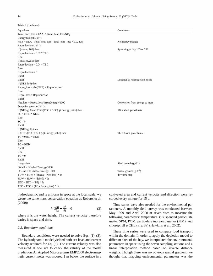
Table 1 (continued)

Equations CommentsTotal_excr_loss = 62.23 * Total_heat_loss/NO2

Energy budget (J d–1)NEB = NEA - Total_heat_loss - Total_excr_loss * 0.02428 Net energy budgetReproduction (J d–1)if (day.eq.165) then Spawning at day 165 or 250Reproduction = 0.07 * TECElseif (day.eq.250) thenReproduction = 0.04 * TECElseReproduction = 0EndifEndif Loss due to reproduction effortif (NEB.lt.0) thenRepro_loss = abs(NEB) + ReproductionElseRepro_loss = ReproductionEndifNet_loss = Repro_loss/tissue2energy/1000 Conversion from energy to massScope for growth (J d–1)if (NEB.gt.0.and.TEC/(TEC + SEC).gt.Energy_ratio) then SG = shell growth rateSG = 0.103 * NEBElseSG = 0Endifif (NEB.gt.0) thenif (TEC/(TEC + SEC).gt.Energy_ratio) then TG = tissue growth rateTG = 0.897 * NEBElseTG = NEBEndifElseTG = 0EndifIntegration Shell growth (g d–1)Dshell = SG/shell2energy/1000Dtissue = TG/tissue2energy/1000 Tissue growth (g d–1)TDW = TDW + (dtissue - Net_loss) * dt dt = time stepSDW = SDW + (dshell) * dtSEC = SEC + (SG) * dtTEC = TEC + (TG - Repro_loss) * dt


quickest and most relevant method to provide test values forthe model at any location of the bay.

2.3. Simulations

Numerical integration of Eqs. (1)–(3) was based on dis-cretization in space and time. The spatial domain was 1000 mand was split into three equivalently sized horizontal boxes toaccount for potential spatial variability, and the time step wasequal to 600 s. The model was successively applied to all thenodes used by the hydrodynamical model (Fig. 3a) (149nodes not counting the nodes at the terrestrial or oceanicboundaries). For each simulation, CHL, POM, PIM, indi-vidual scallop dry weight and total weight were computed for1 year. Simulations started in October, which is the seeding

time (Hawkins et al., 2002). We therefore used our measuredtime series of SPM, POM, CHL, PIM, T to build annualforcing functions starting in October. Guo et al. (1999) de-scribe the lantern net cultivation method in detail but, for ourmodel, it is more relevant to consider the density of individu-als (individuals per m3). We tested two different densities: 0and 50 ind m–3. The null density refers to a case where wesimulated the growth of a single individual without depletionand therefore provides the maximum annual weight. Com-paring the two series of simulations allows the assessment ofthe density effect on the growth. After many sites with differ-ent hydrodynamic and food conditions were simulated, theresults were mapped in order to assess the sensitivity of thedensity effect on the spatial variability of environmentalconditions, as well as produce baywide patterns of seston

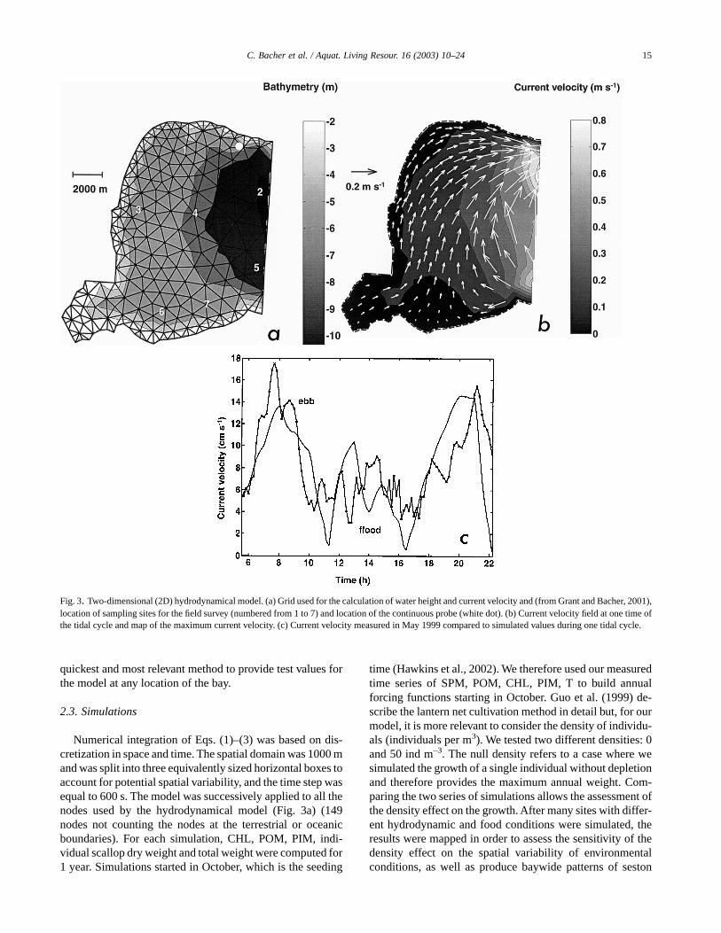
Fig. 3. Two-dimensional (2D) hydrodynamical model. (a) Grid used for the calculation of water height and current velocity and (from Grant and Bacher, 2001),location of sampling sites for the field survey (numbered from 1 to 7) and location of the continuous probe (white dot). (b) Current velocity field at one time ofthe tidal cycle and map of the maximum current velocity. (c) Current velocity measured in May 1999 compared to simulated values during one tidal cycle.


depletion and growth. Depletion factor was defined as theratio between food concentration (e.g. CHL or POM) insidethe spatial domain and at the boundary of the spatial domain.

3. Results

3.1. Field survey

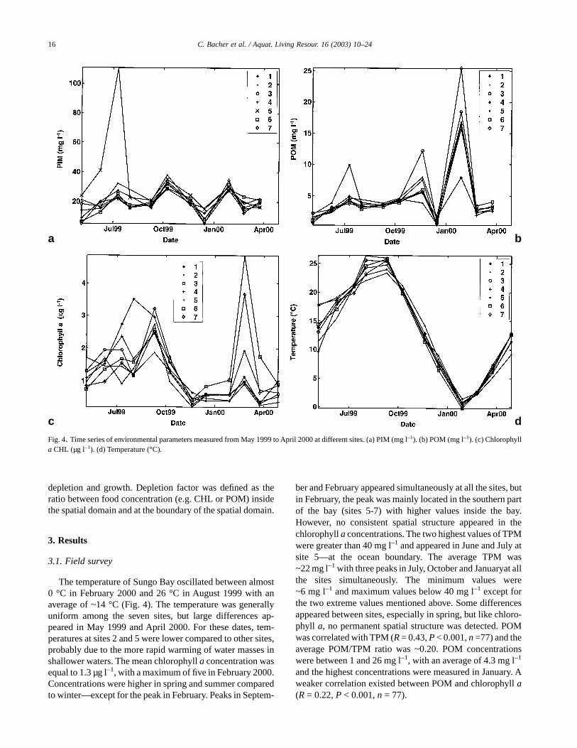
The temperature of Sungo Bay oscillated between almost0 °C in February 2000 and 26 °C in August 1999 with anaverage of ~14 °C (Fig. 4). The temperature was generallyuniform among the seven sites, but large differences ap-peared in May 1999 and April 2000. For these dates, tem-peratures at sites 2 and 5 were lower compared to other sites,probably due to the more rapid warming of water masses inshallower waters. The mean chlorophyll a concentration wasequal to 1.3 µg l–1, with a maximum of five in February 2000.Concentrations were higher in spring and summer comparedto winter—except for the peak in February. Peaks in Septem-

ber and February appeared simultaneously at all the sites, butin February, the peak was mainly located in the southern partof the bay (sites 5-7) with higher values inside the bay.However, no consistent spatial structure appeared in thechlorophyll a concentrations. The two highest values of TPMwere greater than 40 mg l–1 and appeared in June and July atsite 5—at the ocean boundary. The average TPM was~22 mg l–1 with three peaks in July, October and Januaryat allthe sites simultaneously. The minimum values were~6 mg l–1 and maximum values below 40 mg l–1 except forthe two extreme values mentioned above. Some differencesappeared between sites, especially in spring, but like chloro-phyll a, no permanent spatial structure was detected. POMwas correlated with TPM (R = 0.43, P < 0.001, n =77) and theaverage POM/TPM ratio was ~0.20. POM concentrationswere between 1 and 26 mg l–1, with an average of 4.3 mg l–1

and the highest concentrations were measured in January. Aweaker correlation existed between POM and chlorophyll a(R = 0.22, P < 0.001, n = 77).

Fig. 4. Time series of environmental parameters measured from May 1999 to April 2000 at different sites. (a) PIM (mg l–1). (b) POM (mg l–1). (c) Chlorophylla CHL (µg l–1). (d) Temperature (°C).

a b

c d


3.2. Hydrodynamics

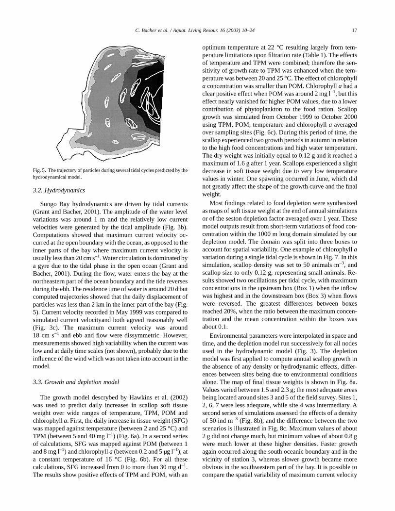
Sungo Bay hydrodynamics are driven by tidal currents(Grant and Bacher, 2001). The amplitude of the water levelvariations was around 1 m and the relatively low currentvelocities were generated by the tidal amplitude (Fig. 3b).Computations showed that maximum current velocity oc-curred at the open boundary with the ocean, as opposed to theinner parts of the bay where maximum current velocity isusually less than 20 cm s–1. Water circulation is dominated bya gyre due to the tidal phase in the open ocean (Grant andBacher, 2001). During the flow, water enters the bay at thenortheastern part of the ocean boundary and the tide reversesduring the ebb. The residence time of water is around 20 d butcomputed trajectories showed that the daily displacement ofparticles was less than 2 km in the inner part of the bay (Fig.5). Current velocity recorded in May 1999 was compared tosimulated current velocityand both agreed reasonably well(Fig. 3c). The maximum current velocity was around18 cm s–1 and ebb and flow were dissymmetric. However,measurements showed high variability when the current waslow and at daily time scales (not shown), probably due to theinfluence of the wind which was not taken into account in themodel.

3.3. Growth and depletion model

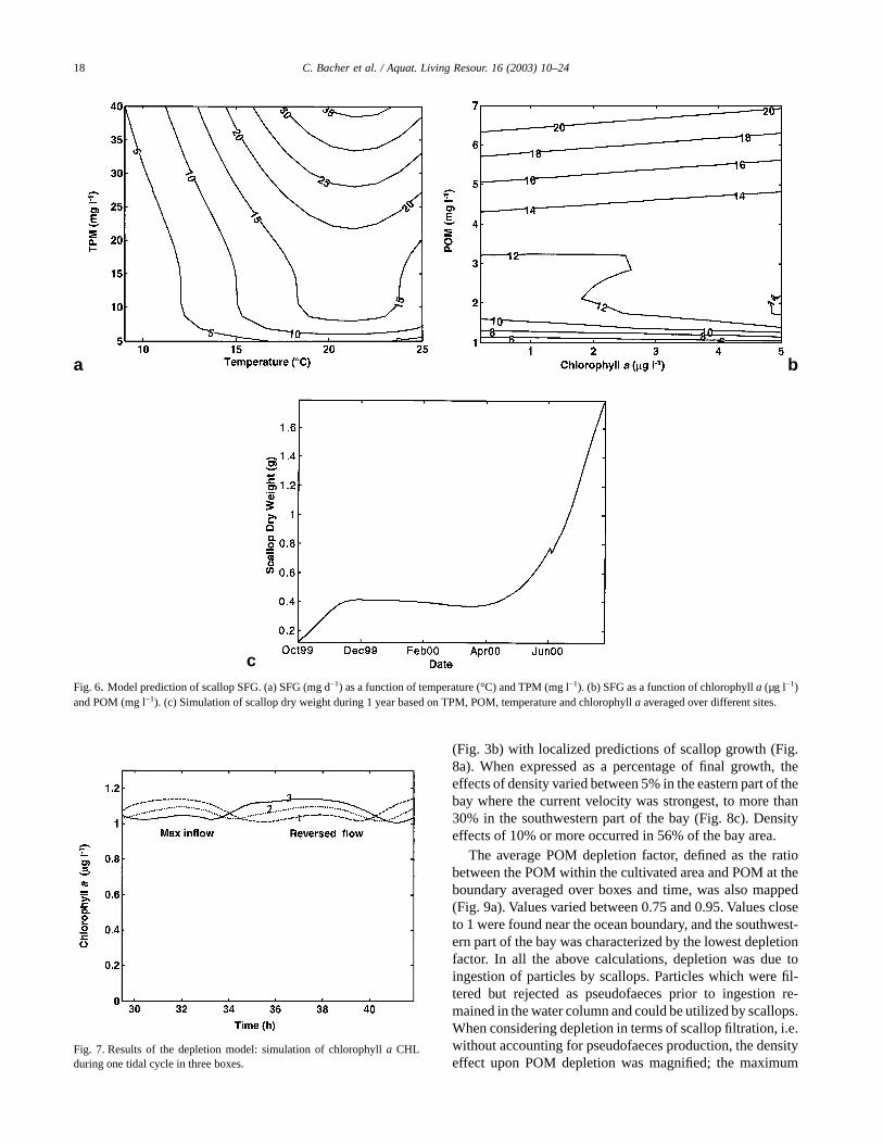
The growth model descrybed by Hawkins et al. (2002)was used to predict daily increases in scallop soft tissueweight over wide ranges of temperature, TPM, POM andchlorophyll a. First, the daily increase in tissue weight (SFG)was mapped against temperature (between 2 and 25 °C) andTPM (between 5 and 40 mg l–1) (Fig. 6a). In a second seriesof calculations, SFG was mapped against POM (between 1and 8 mg l–1) and chlorophyll a (between 0.2 and 5 µg l–1), ata constant temperature of 16 °C (Fig. 6b). For all thesecalculations, SFG increased from 0 to more than 30 mg d–1.The results show positive effects of TPM and POM, with an

optimum temperature at 22 °C resulting largely from tem-perature limitations upon filtration rate (Table 1). The effectsof temperature and TPM were combined; therefore the sen-sitivity of growth rate to TPM was enhanced when the tem-perature was between 20 and 25 °C. The effect of chlorophylla concentration was smaller than POM. Chlorophyll a had aclear positive effect when POM was around 2 mg l–1, but thiseffect nearly vanished for higher POM values, due to a lowercontribution of phytoplankton to the food ration. Scallopgrowth was simulated from October 1999 to October 2000using TPM, POM, temperature and chlorophyll a averagedover sampling sites (Fig. 6c). During this period of time, thescallop experienced two growth periods in autumn in relationto the high food concentrations and high water temperature.The dry weight was initially equal to 0.12 g and it reached amaximum of 1.6 g after 1 year. Scallops experienced a slightdecrease in soft tissue weight due to very low temperaturevalues in winter. One spawning occurred in June, which didnot greatly affect the shape of the growth curve and the finalweight.

Most findings related to food depletion were synthesizedas maps of soft tissue weight at the end of annual simulationsor of the seston depletion factor averaged over 1 year. Thesemodel outputs result from short-term variations of food con-centration within the 1000 m long domain simulated by ourdepletion model. The domain was split into three boxes toaccount for spatial variability. One example of chlorophyll avariation during a single tidal cycle is shown in Fig. 7. In thissimulation, scallop density was set to 50 animals m–3, andscallop size to only 0.12 g, representing small animals. Re-sults showed two oscillations per tidal cycle, with maximumconcentrations in the upstream box (Box 1) when the inflowwas highest and in the downstream box (Box 3) when flowswere reversed. The greatest differences between boxesreached 20%, when the ratio between the maximum concen-tration and the mean concentration within the boxes wasabout 0.1.

Environmental parameters were interpolated in space andtime, and the depletion model run successively for all nodesused in the hydrodynamic model (Fig. 3). The depletionmodel was first applied to compute annual scallop growth inthe absence of any density or hydrodynamic effects, differ-ences between sites being due to environmental conditionsalone. The map of final tissue weights is shown in Fig. 8a.Values varied between 1.5 and 2.3 g; the most adequate areasbeing located around sites 3 and 5 of the field survey. Sites 1,2, 6, 7 were less adequate, while site 4 was intermediary. Asecond series of simulations assessed the effects of a densityof 50 ind m–3 (Fig. 8b), and the difference between the twoscenarios is illustrated in Fig. 8c. Maximum values of about2 g did not change much, but minimum values of about 0.8 gwere much lower at these higher densities. Faster growthagain occurred along the south oceanic boundary and in thevicinity of station 3, whereas slower growth became moreobvious in the southwestern part of the bay. It is possible tocompare the spatial variability of maximum current velocity

Fig. 5. The trajectory of particles during several tidal cycles predicted by thehydrodynamical model.


(Fig. 3b) with localized predictions of scallop growth (Fig.8a). When expressed as a percentage of final growth, theeffects of density varied between 5% in the eastern part of thebay where the current velocity was strongest, to more than30% in the southwestern part of the bay (Fig. 8c). Densityeffects of 10% or more occurred in 56% of the bay area.

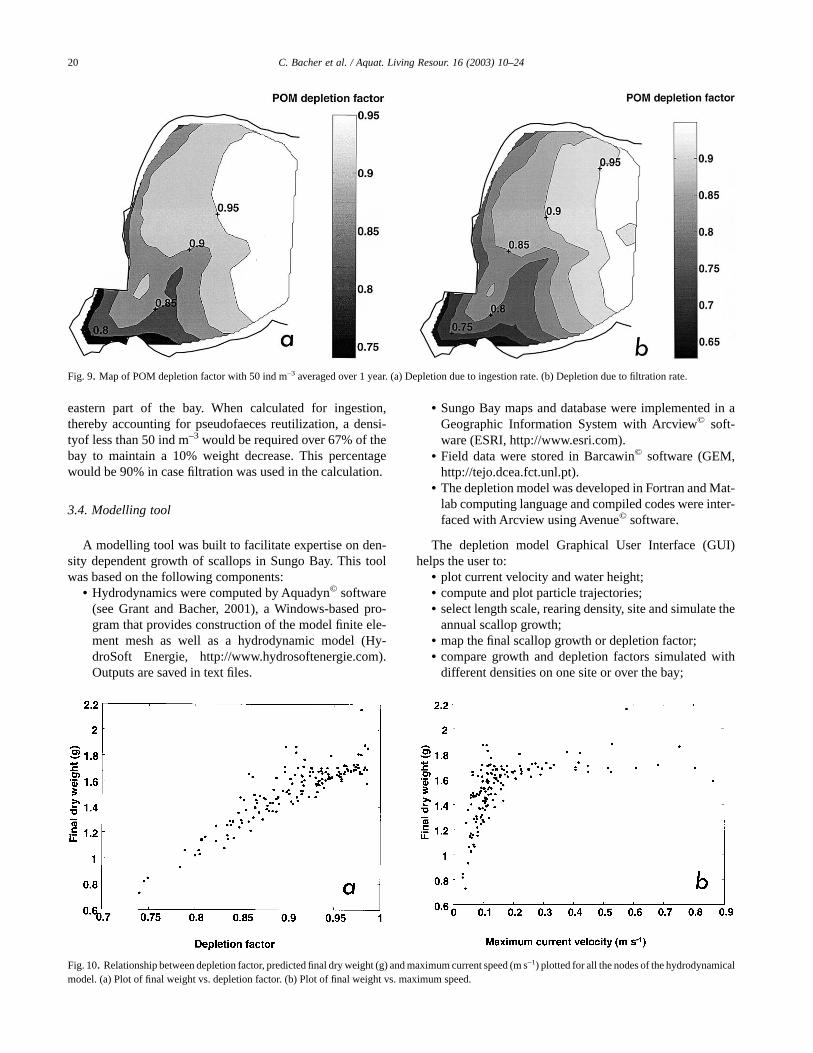
The average POM depletion factor, defined as the ratiobetween the POM within the cultivated area and POM at theboundary averaged over boxes and time, was also mapped(Fig. 9a). Values varied between 0.75 and 0.95. Values closeto 1 were found near the ocean boundary, and the southwest-ern part of the bay was characterized by the lowest depletionfactor. In all the above calculations, depletion was due toingestion of particles by scallops. Particles which were fil-tered but rejected as pseudofaeces prior to ingestion re-mained in the water column and could be utilized by scallops.When considering depletion in terms of scallop filtration, i.e.without accounting for pseudofaeces production, the densityeffect upon POM depletion was magnified; the maximum

Fig. 6. Model prediction of scallop SFG. (a) SFG (mg d–1) as a function of temperature (°C) and TPM (mg l–1). (b) SFG as a function of chlorophyll a (µg l–1)and POM (mg l–1). (c) Simulation of scallop dry weight during 1 year based on TPM, POM, temperature and chlorophyll a averaged over different sites.

a b

c

Fig. 7. Results of the depletion model: simulation of chlorophyll a CHLduring one tidal cycle in three boxes.


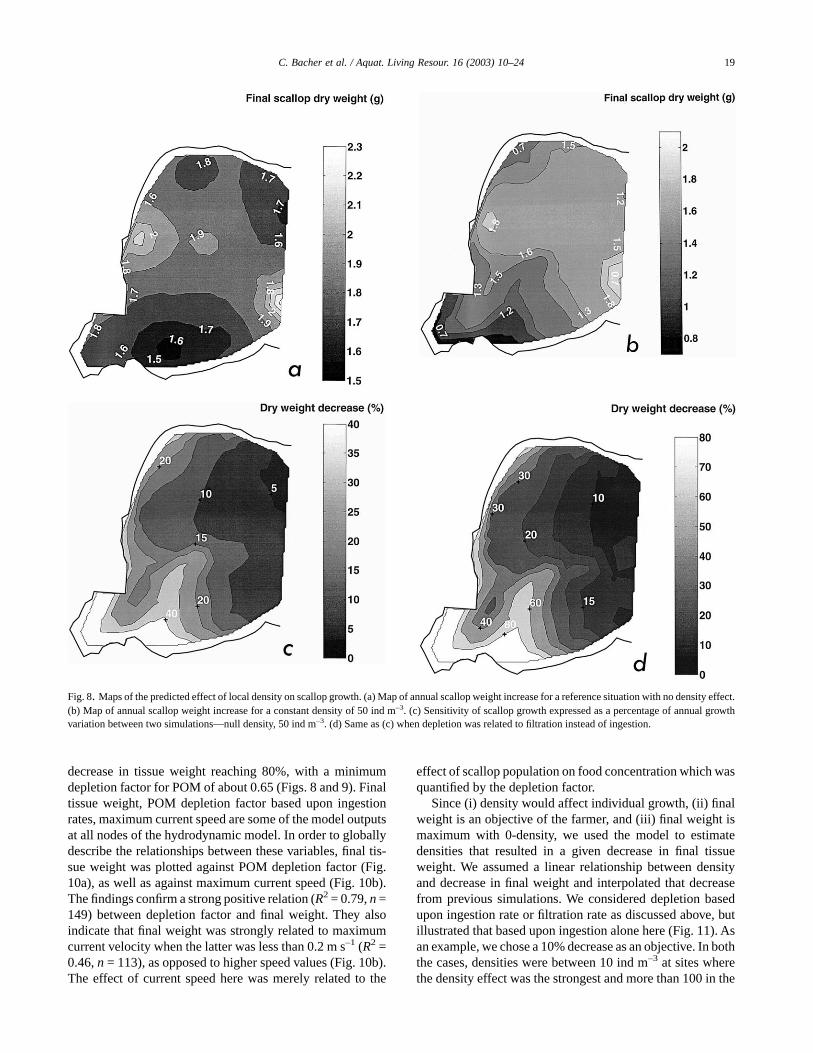
decrease in tissue weight reaching 80%, with a minimumdepletion factor for POM of about 0.65 (Figs. 8 and 9). Finaltissue weight, POM depletion factor based upon ingestionrates, maximum current speed are some of the model outputsat all nodes of the hydrodynamic model. In order to globallydescribe the relationships between these variables, final tis-sue weight was plotted against POM depletion factor (Fig.10a), as well as against maximum current speed (Fig. 10b).The findings confirm a strong positive relation (R2 = 0.79, n =149) between depletion factor and final weight. They alsoindicate that final weight was strongly related to maximumcurrent velocity when the latter was less than 0.2 m s–1 (R2 =0.46, n = 113), as opposed to higher speed values (Fig. 10b).The effect of current speed here was merely related to the

effect of scallop population on food concentration which wasquantified by the depletion factor.

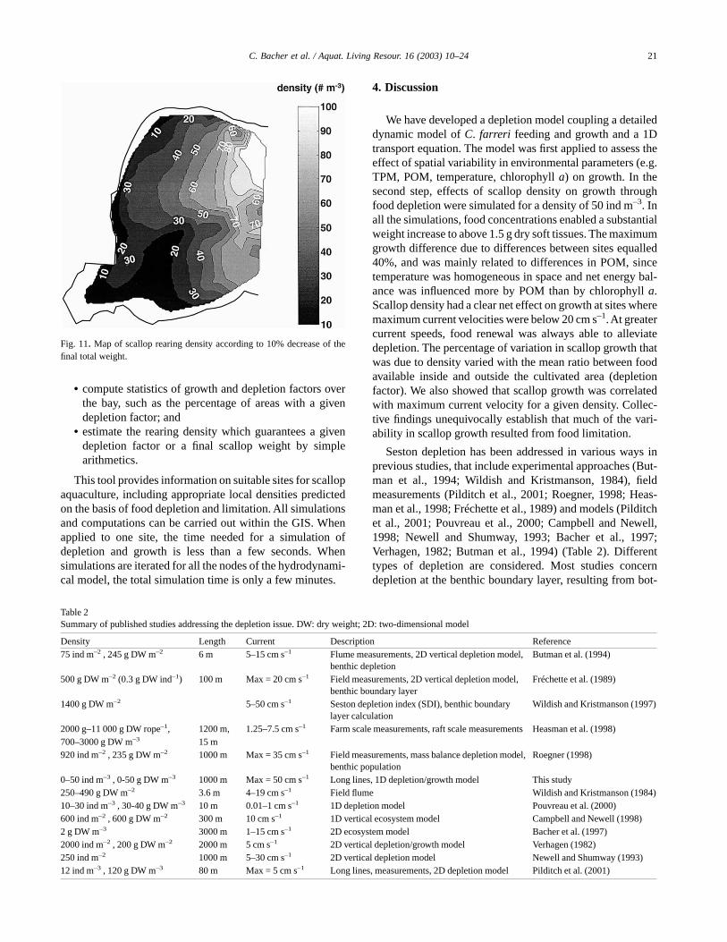
Since (i) density would affect individual growth, (ii) finalweight is an objective of the farmer, and (iii) final weight ismaximum with 0-density, we used the model to estimatedensities that resulted in a given decrease in final tissueweight. We assumed a linear relationship between densityand decrease in final weight and interpolated that decreasefrom previous simulations. We considered depletion basedupon ingestion rate or filtration rate as discussed above, butillustrated that based upon ingestion alone here (Fig. 11). Asan example, we chose a 10% decrease as an objective. In boththe cases, densities were between 10 ind m–3 at sites wherethe density effect was the strongest and more than 100 in the

Fig. 8. Maps of the predicted effect of local density on scallop growth. (a) Map of annual scallop weight increase for a reference situation with no density effect.(b) Map of annual scallop weight increase for a constant density of 50 ind m–3. (c) Sensitivity of scallop growth expressed as a percentage of annual growthvariation between two simulations—null density, 50 ind m–3. (d) Same as (c) when depletion was related to filtration instead of ingestion.


eastern part of the bay. When calculated for ingestion,thereby accounting for pseudofaeces reutilization, a densi-tyof less than 50 ind m–3 would be required over 67% of thebay to maintain a 10% weight decrease. This percentagewould be 90% in case filtration was used in the calculation.

3.4. Modelling tool

A modelling tool was built to facilitate expertise on den-sity dependent growth of scallops in Sungo Bay. This toolwas based on the following components:

• Hydrodynamics were computed by Aquadyn© software(see Grant and Bacher, 2001), a Windows-based pro-gram that provides construction of the model finite ele-ment mesh as well as a hydrodynamic model (Hy-droSoft Energie, http://www.hydrosoftenergie.com).Outputs are saved in text files.

• Sungo Bay maps and database were implemented in aGeographic Information System with Arcview© soft-ware (ESRI, http://www.esri.com).

• Field data were stored in Barcawin© software (GEM,http://tejo.dcea.fct.unl.pt).

• The depletion model was developed in Fortran and Mat-lab computing language and compiled codes were inter-faced with Arcview using Avenue© software.

The depletion model Graphical User Interface (GUI)helps the user to:

• plot current velocity and water height;• compute and plot particle trajectories;• select length scale, rearing density, site and simulate the

annual scallop growth;• map the final scallop growth or depletion factor;• compare growth and depletion factors simulated with

different densities on one site or over the bay;

Fig. 9. Map of POM depletion factor with 50 ind m–3 averaged over 1 year. (a) Depletion due to ingestion rate. (b) Depletion due to filtration rate.

Fig. 10. Relationship between depletion factor, predicted final dry weight (g) and maximum current speed (m s–1) plotted for all the nodes of the hydrodynamicalmodel. (a) Plot of final weight vs. depletion factor. (b) Plot of final weight vs. maximum speed.


• compute statistics of growth and depletion factors overthe bay, such as the percentage of areas with a givendepletion factor; and

• estimate the rearing density which guarantees a givendepletion factor or a final scallop weight by simplearithmetics.

This tool provides information on suitable sites for scallopaquaculture, including appropriate local densities predictedon the basis of food depletion and limitation. All simulationsand computations can be carried out within the GIS. Whenapplied to one site, the time needed for a simulation ofdepletion and growth is less than a few seconds. Whensimulations are iterated for all the nodes of the hydrodynami-cal model, the total simulation time is only a few minutes.

4. Discussion

We have developed a depletion model coupling a detaileddynamic model of C. farreri feeding and growth and a 1Dtransport equation. The model was first applied to assess theeffect of spatial variability in environmental parameters (e.g.TPM, POM, temperature, chlorophyll a) on growth. In thesecond step, effects of scallop density on growth throughfood depletion were simulated for a density of 50 ind m–3. Inall the simulations, food concentrations enabled a substantialweight increase to above 1.5 g dry soft tissues. The maximumgrowth difference due to differences between sites equalled40%, and was mainly related to differences in POM, sincetemperature was homogeneous in space and net energy bal-ance was influenced more by POM than by chlorophyll a.Scallop density had a clear net effect on growth at sites wheremaximum current velocities were below 20 cm s–1.At greatercurrent speeds, food renewal was always able to alleviatedepletion. The percentage of variation in scallop growth thatwas due to density varied with the mean ratio between foodavailable inside and outside the cultivated area (depletionfactor). We also showed that scallop growth was correlatedwith maximum current velocity for a given density. Collec-tive findings unequivocally establish that much of the vari-ability in scallop growth resulted from food limitation.

Seston depletion has been addressed in various ways inprevious studies, that include experimental approaches (But-man et al., 1994; Wildish and Kristmanson, 1984), fieldmeasurements (Pilditch et al., 2001; Roegner, 1998; Heas-man et al., 1998; Fréchette et al., 1989) and models (Pilditchet al., 2001; Pouvreau et al., 2000; Campbell and Newell,1998; Newell and Shumway, 1993; Bacher et al., 1997;Verhagen, 1982; Butman et al., 1994) (Table 2). Differenttypes of depletion are considered. Most studies concerndepletion at the benthic boundary layer, resulting from bot-

Fig. 11. Map of scallop rearing density according to 10% decrease of thefinal total weight.

Table 2Summary of published studies addressing the depletion issue. DW: dry weight; 2D: two-dimensional model

Density Length Current Description Reference75 ind m–2 , 245 g DW m–2 6 m 5–15 cm s–1 Flume measurements, 2D vertical depletion model,

benthic depletionButman et al. (1994)

500 g DW m–2 (0.3 g DW ind–1) 100 m Max = 20 cm s–1 Field measurements, 2D vertical depletion model,benthic boundary layer

Fréchette et al. (1989)

1400 g DW m–2 5–50 cm s–1 Seston depletion index (SDI), benthic boundarylayer calculation

Wildish and Kristmanson (1997)

2000 g–11 000 g DW rope–1, 1200 m, 1.25–7.5 cm s–1 Farm scale measurements, raft scale measurements Heasman et al. (1998)700–3000 g DW m–3 15 m920 ind m–2 , 235 g DW m–2 1000 m Max = 35 cm s–1 Field measurements, mass balance depletion model,

benthic populationRoegner (1998)

0–50 ind m–3 , 0-50 g DW m–3 1000 m Max = 50 cm s–1 Long lines, 1D depletion/growth model This study250–490 g DW m–2 3.6 m 4–19 cm s–1 Field flume Wildish and Kristmanson (1984)10–30 ind m–3 , 30-40 g DW m–3 10 m 0.01–1 cm s–1 1D depletion model Pouvreau et al. (2000)600 ind m–2 , 600 g DW m–2 300 m 10 cm s–1 1D vertical ecosystem model Campbell and Newell (1998)2 g DW m–3 3000 m 1–15 cm s–1 2D ecosystem model Bacher et al. (1997)2000 ind m–2 , 200 g DW m–2 2000 m 5 cm s–1 2D vertical depletion/growth model Verhagen (1982)250 ind m–2 1000 m 5–30 cm s–1 2D vertical depletion model Newell and Shumway (1993)12 ind m–3 , 120 g DW m–3 80 m Max = 5 cm s–1 Long lines, measurements, 2D depletion model Pilditch et al. (2001)


tom culture or benthic bivalve populations (Campbell andNewell, 1998; Newell and Shumway, 1993; Roegner, 1998;Verhagen, 1982; Butman et al., 1984; Wildish and Kristman-son, 1984, 1997). A few studies deal with cultivated specieson rafts or long-lines (Bacher et al., 1997; Pouvreau et al.,2000; Heasman et al., 1998; Pilditch et al., 2001). Scalesencompass a wide range of values. Lengths of the studiedsystems range from 6 m in experimental studies to more than1000 m. For benthic populations, the density of studiedsystems ranges from 75 to 2000 ind m–2, corresponding toranges from 200 to 1 400 g soft tissue m–2. For suspendedcultures, the density of studied systems ranges between 2 and700 g soft tissue m–3. Minimum current velocities range fromless than 1 to 35 cm s–1 (Table 2). All studies stress that fooddepletion may limit production, depending on the nature ofthe population (benthic, suspended), as well as scales ofcurrent velocity, density and length. Depletion would arise atspatial scales over a few kilometres when density is low orcurrent velocity is high (Bacher et al., 1997; Newell andShumway, 1993) and local depletion would not occur atsmaller distances. Our calculations clearly confirmed theimportance of depletion in the case of a bay with a largerange of hydrodynamical conditions, at a scale of 1000 m andwith a low density of animals. Our choice of 1000 m lengthstemmed from the mixing length defined from trajectorysimulations. This guaranteed mixing of particles when watermass exited the 1000 m area, so that boundary conditionswere correctly prescribed. Depletion would certainly occurat shorter lengths, but would be weaker unless densities aremuch higher, such as in raft culture (Heasman et al., 1998).For larger domains, we would have to consider other pro-cesses such as primary production, which would signifi-cantly compensate for the ingestion of particles by scallops.Here, we have demonstrated that managing rearing density ata 1000 m scale according to food supply and depletion aloneprovides useful indications on how to optimize individualgrowth.

Measuring food depletion, as well as its effect on growthand production, is problematic in the field. Fréchette et al.(1989) and Newell and Shumway (1993) demonstrated re-duction in phytoplankton concentration near benthic bound-ary layers. In the water column, Ogilvie et al. (2000) assessedthe effect of mussels on nutrients and chlorophyll a concen-trations within farms, finding depletion when phytoplanktonconcentrations were low. Roegner (1998) measured fooddepletion in an estuary in some occasions though flux calcu-lations always showed a significant effect of clearance ratedue to benthic filter-feeders. Heasman et al. (1998) relateddifferences in mussel growth to high depletion factors mea-sured within densely cultivated rafts. Pilditch et al. (2001)did not observe reduction in seston concentration at a smallscale, but expected a significant depletion if the lease areawere to be extended. The reasons generally invoked fordifficulty in measuring depletion are related either to scale(density, length, current velocity) or variability of environ-mental conditions. In the present study, it was quite clear that

environmental variability would mask the measurement ofdepletion in the field. Records of current velocity over sev-eral days were highly variable, probably due to the wind,with associated resuspension of organic and inorganic par-ticles. On large scales, measurements of depletion wouldrequire intensive sampling in time and space, optimally usinglong-term moored instruments.

Several sources of uncertainty were apparent in our calcu-lations. Measurements of current velocity revealed somevariability, which would affect predictions of depletion andgrowth. However, hydrodynamics were dominated by thetide, which generated a regular and consistent pattern. Moreuncertainty is expected from the estimation of food availabil-ity. Previous studies (Fang, comm. pers.) showed that inter-annual levels of POM, TPM, and chlorophyll a have beenchanging over the past 20 years, probably due to changes inland use and aquaculture practices. Our sampling strategybased on a monthly field survey did not account for short-term variability related to tides, nor for changes in meteoro-logical conditions on which information was lacking. Wewere forced to interpolate to supply sufficient data. Modeloutputs would certainly have benefited from a larger dataset,more accurately representing temporal and spatial variationsof the forcing functions. Finally, outputs of the depletionmodel were sensitive to how we formulated the sink ofparticles, whether through ingestion, thus allowing for thereutilization of rejected matter, or through filtration, in whichcase, all the filtered particles were no longer available. Usingingestion minimized depletion, including effects of densityon growth. It is likely that a significant fraction of pseud-ofaeces becomes available for reutilization following breakup and resuspension. One way to resolve this uncertaintywould be to measure the sinking rate of pseudofaeces incultivated areas, and parameterize a biodeposition term in thedepletion model.

Very high rearing densities would affect mortality andproduction (Fréchette et al., 2000), but we kept densities lowenough in our calculations to assume no effect. We alsoassumed that primary production was negligible at the scalewe chose. This can be acceptable when renewal time is short,which is presumably true in most parts of Sungo Bay. Forinstance, a 1000 m long domain is renewed every 3 h whenthe current speed is 10 cm s–1. It can also be argued thatphytoplankton is only a fraction of food ration and thatneglecting phytoplankton production would not affect scal-lop growth. If really needed, source terms could, however,easily be added to Eq. (1) using phytoplankton turnover ratesestimated from field measurements. Another potential im-provement in our calculation concerns interactions betweencurrent velocity and filter-feeders, which were neglected.Grant and Bacher (2001), Boyd and Heasman (1998) andPilditch et al. (2001) established that long lines or raftsmodify the current velocity within cultivated areas, resultingin increased food depletion. In addition, Wildish and Krist-manson (1997) reported as to how scallop filter feeding maybe inhibited at higher currents, though the effect of flow on


growth can be compensated when flow is periodic. Due totheir complexity, both positive and negative effects are diffi-cult to predict and have been neglected here, but we suggestthat our predictions are a valid and quantitative approach forguiding aquaculture practice. From this perspective and toour knowledge, our model is the most spatially explicit withrespect to modelling of density effects on aquaculture pro-duction ever attempted.

Our work was undertaken with the objective of helping todevelop tools for the management of aquaculture. Campbelland Newell (1998) simulated local interactions betweenmussel beds and ecosystem processes, to provide recommen-dations on seeding density and timing. Pastres et al. (2001)also used a detailed ecosystem model to identify suitablesites for clam production in the lagoon of Venice. Othermodels have been developed to assess carrying capacity atthe scale of the ecosystem (Raillard and Menesguen, 1994;Dowd, 1997; Bacher et al., 1998; Ferreira et al., 1998). Adifferent approach was proposed by Arnold et al. (2000) toselect lease sites for clam aquaculture in Florida, using mul-tiple criteria based on the limitation of culture impact, waterquality and associated spatial requirements. The novelty ofour approach has been in coupling bivalve growth and fooddepletion at a site of intensive aquaculture, where identifyingsustainable rearing densities is a major challenge. Fooddepletion factors, suitable rearing densities and expectedindividual growth rates can be superimposed with spatialinformation in a GIS, helping in the management of scallopaquaculture. Concepts (depletion), methods (coupling hy-drodynamics and ecophysiology), and the underlying frame-work (GIS) are all generic, and can be applied to differentsites where local interactions are important. Whilst of un-doubted application at the farm scale, more comprehensivemodels will be required to simulate processes at larger eco-system scales.

Acknowledgements

This work was supported by the INCO-DC project “Car-rying capacity and impact of aquaculture on the environmentin Chinese bays” contract number ERBIC18CT980291, EU.

References

Arnold, W.S., White, M.W., Norris, H.A., Berrigan, M.E., 2000. Hard clam(Mercenaria spp.) aquaculture in Florida, USA: geographic informationsystem applications to lease site selection. Aquacult. Eng. 23, 203–231.

Bacher, C., Duarte, P., Ferreira, J.G., Héral, M., Raillard, O., 1998. Assess-ment and comparison of the Marennes-Oléron Bay (France) and Carling-ford Lough (Ireland) carrying capacity with ecosystem models. Aquat.Ecol. 31, 379–394.

Bacher, C., Millet, B., Vaquer, A., 1997. Modélisation de l’ impact desmollusques cultivés sur la biomasse phytoplanctonique de l’étang deThau (France). C.R. Acad. Sci. Paris, Sér. III 320, 73–81.

Barillé, L., Héral, M., Barillé-Boyer, A.L., 1997. Modélisation del’écophysiologie de l’huître Crassostrea gigas dans un environnementestuarien. Aquat. Living Resour. 10, 31–48.

Boyd, A.J., Heasman, K.G., 1998. Shellfish mariculture in the Benguelasystem: water flow patterns within a mussel farm in Saldanha Bay, SouthAfrica. J. Shellfish Res. 17, 25–32.

Butman, C.A., Fréchette, M., Geyer, W.R., Starczak, V.R., 1994. Flumeexperiments on food supply to the blue mussel Mytilus edulis L. as afunction of boundary layer flow. Limnol.. Oceanogr. 39, 1755–1768.

Campbell, D.E., Newell, C.R., 1998. MUSMOD a production model forbottom culture of the blue mussel, Mytilus edulis L. J. Exp. Mar. Biol.Ecol. 219, 171–203.

Dame, R.F., 1993. Bivalve Filter Feeders in Estuarine and Coastal Ecosys-tem Processes. Springer-Verlag, 1993, Berlin, pp. 579.

Dowd, M., 1997. On predicting the growth of cultured bivalves. Ecol.Model. 104, 113–131.

Fang, J., Sun, H., Kuang, S., Sun,Y., Zhou, S., Song,Y., et al., 1996. Study onthe carrying capacity of Sanggou Bay for the culture of scallop Chlamysfarreri. Mar. Fish. Res. 17, 18–31 (in Chinese).

Ferreira, J.G., Duarte, P., Ball, B., 1998. Trophic capacity of CarlingfordLough for oyster culture—analysis by ecological modelling. Aquat.Ecol. 31, 361–378.

Fréchette, M., Butman, C.A., Geyer, W.R., 1989. The importance of bound-ary layer flows in supplying phytoplankton to the suspension feeder,Mytilus edulis L. Limnol. Oceanogr. 34, 19–36.

Fréchette, M., Gaudet, M., Vigneau, S., 2000. Estimating optimal populationdensity for intermediate culture of scallops in spat collector bags. Aquac-ulture 183, 105–124.

Grant, J., 1996. The relationship of bioenergetics and the environment to thefield growth of culture bivalves. Aquaculture 200, 239–256.

Grant, J., Bacher, C., 1998. Comparative models of mussel bioenergetics andtheir validation at field culture sites. J. Exp. Mar. Biol. Ecol. 219, 21–44.

Grant, J., Bacher, C., 2001. A numerical model of flow modification inducedby suspended aquaculture in a Chinese bay. Can. J. Fish. Aquat. Sci. 58,1003–1011.

Guo, X., Ford, S., Zhang, F., 1999. Molluscan aquaculture in China. J.Shellfish Res. 18, 19–32.

Hawkins, A.J.S., Duarte, P., Fang, J.G., Pascoe, P.L., Zhang, J.H.,Zhang, X.L., et al., 2002. A functional simulation of responsive filter-feeding and growth in bivalve shellfish, configured and validated for thescallop Chlamys farreri during culture in China. J. Exp. Mar. Biol. Ecol.281, 13–40.

Heasman, K.G., Pitcher, G.C., McQuaid, C.D., Hecht, T., 1998. Shellfishmariculture in the Benguela system: raft culture of Mytilus galloprovin-cialis and the effect of rope spacing on food extraction, growth rate,production, and condition of mussels. J. Shellfish Res. 17, 33–39.

Incze, L.S., Lutz, R.A., True, E., 1981. Modelling carrying capacity forbivalve molluscs in open, suspended-culture systems. J. World Maricult.Soc. 12, 143–155.

Nath, S.S., Bolte, J.P., Ross, L.G., Aguilar-Manjarrez, J., 2000. Applicationsof geographical information system (GIS) for spatial decision support inaquaculture. Aquacult. Eng. 23, 233–278.

Newell, C.R., Shumway, S.E., 1993. Grazing of natural particulates bybivalves molluscs: a spatial and temporal perspective. In: Dame, R.F.(Ed.), Bivalve Filter Feeders in Estuarine and Coastal Ecosystem Pro-cesses. Springer-Verlag, Berlin, 1993, Berlin.

Ogilvie, S.C., Ross, A.H., Schiel, D.R., 2000. Phytoplankton biomass asso-ciated with mussel farms in Beatrix Bay, New Zealand. Aquaculture 181,71–80.

Pastres, R., Solidoro, C., Cossarini, G., Melaku Canu, D., Dejak, C., 2001.Managing the rearing of Tapes philippinarum in the lagoon of Venice: adecision support system. Ecol. Model. 138, 231–245.

Pilditch, C.A., Grant, J., Bryan, K.R., 2001. Seston supply to sea scallops(Placopecten magellanicus) in suspended culture. Can. J. Fish. Aquat.Sci. 58, 241–253.

Pouvreau, S., Bacher, C., Héral, M., 2000. Ecophysiological model ofgrowth and reproduction of the black pearl oyster, Pinctadamargaritifera: potential applications for pearl farming in French Polyne-sia. Aquaculture 186, 117–144.


Powell, E.N., Hofmann, E.E., Klinck, J.M., Ray, S.M., 1992. Modellingoyster populations. I. A commentaryon filtration rate. Is faster alwaysbetter? J. Shellfish Res. 11, 387–398.

Raillard, O., Deslous-Paoli, J.M., Héral, M., Razet, D., 1993. Modélisationdu comportement nutritionnel et de la croissance de l’huître japonaiseCrassostrea gigas. Oceanol. Acta 16, 73–82.

Raillard, O., Menesguen, A., 1994. An ecosystem box model for estimatingthe carrying capacity of a macrotidal shellfish system. Mar. Ecol. Prog.Ser. 115, 117–130.

Ren, J.S., Ross, A.H., 2001. A dynamic energy budget model of the Pacificoyster Crassostrea gigas. Ecol. Model. 142, 105–120.

Roberts, W., Le Hir, P., Whitehouse, R.J.S., 2000. Investigation using simplemathematical models of the effect of tidal currents and waves on theprofile shape of intertidal mudflats. Cont. Shelf Res. 20, 1079–1097.

Roegner, G.C., 1998. Hydrodynamic control of supply of suspended chlo-rophyll a to infaunal estuarine bivalves. Estuar. Coast. Shelf Sci. 47,369–384.

Scholten, H., Smaal, A.C., 1998. Responses of Mytilus edulis L. to varyingfood concentrations: testing EMMY, an ecophysiological model. J. Exp.Mar. Biol. Ecol. 219, 217–239.

Solidoro, C., Pastres, R., Melaku Canu, D., Pellizzato, M., Rossi, R., 2000.Modelling the growth of Tapes philippinarum in Northern Adriaticlagoons. Mar. Ecol. Prog. Ser. 199, 137–148.

Verhagen, J.H.G., 1982. A distribution and population model of the musselMytilus edulis in lake Grevelingen. Third International Conference onState-of-the-Art in Ecological Modelling, Colorado State University,May 24–28, 1982, pp. 373–383.

Wildish, D., Kristmanson, D., 1984. Importance to mussels of the benthicboundary layer. Can. J. Fish. Aquat. Sci. 41, 1618–1625.

Wildish, D., Kristmanson, D., 1997. Benthic Suspension Feeders and Flow.Cambridge University Press, 1997, New York.


modelling the effect of food depletion on scallop growth in sungo bay (china

Documents