Modeling visual search using three-parameter probabilityfunctions in a hierarchical Bayesian framework

Yi-Shin Lin & Dietmar Heinke & Glyn W. Humphreys

Published online: 13 February 2015# The Psychonomic Society, Inc. 2015

Abstract In this study, we applied Bayesian-based distribu-tional analyses to examine the shapes of response time (RT)distributions in three visual search paradigms, which varied intask difficulty. In further analyses we investigated two com-mon observations in visual search—the effects of display sizeand of variations in search efficiency across different taskconditions—following a design that had been used in previousstudies (Palmer, Horowitz, Torralba, & Wolfe, Journal ofExperimental Psychology: Human Perception andPerformance, 37, 58–71, 2011; Wolfe, Palmer, & Horowitz,Vision Research, 50, 1304–1311, 2010) in which parametersof the response distributions were measured. Our studyshowed that the distributional parameters in an experimentalcondition can be reliably estimated by moderate sample sizeswhen Monte Carlo simulation techniques are applied. Moreimportantly, by analyzing trial RTs, we were able to extractparadigm-dependent shape changes in the RT distributionsthat could be accounted for by using the EZ2 diffusion model.The study showed that Bayesian-based RT distribution analy-ses can provide an important means to investigate the under-lying cognitive processes in search, including stimulus group-ing and the bottom-up guidance of attention.

Keywords Bayesianmodeling . Visual search . Responsetimemodels

Distributional analyses are becoming an increasingly popularmethod of analyzing performance in cognitive tasks (e.g.,Balota & Yap, 2011; Heathcote, Popiel, & Mewhort, 1991;Hockley & Corballis, 1982; Ratcliff & Murdock, 1976; Sui &Humphreys, 2013; Tse & Altarriba, 2012). When comparedwith analyses based onmean performance, distributional anal-yses potentially allow a more detailed assessment of the un-derlying processes that lead to a final decision. In particular ithas long been noted that response time (RT) data frequentlyshow a positively skewed, unimodal distribution (Luce, 1986;Van Zandt, 2000). Distributional analyses begin to allow us todecompose such skewed data and to address the processes thatcontribute to different parts of the RT function. One approachto this is through hierarchical Bayesian modeling (HBM), amethod that blends Bayesian statistics and hierarchical model-ing. The latter technique uses separate regressors to assessvariations across trial RTs collected from a participant by es-timating regression coefficients, contrary to conventionalsingle-level analysis of variance (ANOVA) models, whichdirectly use RT means as dependent variables. The hierarchi-cal modeling then carries on assessing the coefficient varia-tions across participants at the second level, accounting forindividual differences. One direct advantage of the hierarchi-cal method is that variation across trials can be described by apositively skewed distribution (or other distributions, as ana-lysts wish), in contrast to the Gaussian distribution implicitlyadopted by a single-level ANOVA model (which works di-rectly on the second level of the hierarchical method). Theflexibility to choose an underlying distribution liberates ana-lysts from using statistics derived from the Gaussian distribu-tion to represent each participant’s performance in an experi-mental condition, since a Gaussian assumption may not beappropriate, given positively skewed RT distributions.

Hierarchical modeling typically relies on point estimation,which itself depends on the critical assumption of the inde-pendence of random sampling—making performance highly

Y.<S. Lin (*) :D. HeinkeSchool of Psychology, University of Birmingham, Edgbaston, B152TT Birmingham, UKe-mail: yxl193@bham.ac.uk

G. W. Humphreys (*)Department of Experimental Psychology, University of Oxford,South Parks Road, Oxford OX1 3UD, UKe-mail: glyn.humphreys@psy.ox.ac.uk

Atten Percept Psychophys (2015) 77:985–1010DOI 10.3758/s13414-014-0825-x

sensitive to the sample size. Hierarchical modeling may per-form less than optimally when, relative to the number of esti-mated parameters, the trial numbers are too few to account forthe parameter uncertainties at each hierarchical level (Gelman& Hill, 2007). This is possible when a non-Gaussian distribu-tion is used to estimate the parameters for each participantseparately in a hierarchical manner. For example, a data setwith ten participants, when using an ex-Gaussian distribution(fully described by three parameters), estimates simultaneous-ly at least 30 (3 × 10) parameters, each of which should bederived from a distribution with an appropriate uncertaintydescription (i.e., parameters for variability). This is assumingthat only one experimental condition is tested. It follows thatsmall trial numbers within an experimental condition mayresult in biased uncertainty estimates, which render the effortof adapting hierarchical modeling in vain. Bayesian statisticsis one of the solutions to the problem of point estimationinherent in the conventional approach. Building on the natureof the hierarchical structure of parameter estimations,Bayesian statistics conceptualize each parameter at one levelas an estimate from a prior distribution. On the basis ofBayes’s theorem, the outputs of prior distributions can thenbe used to calculate posterior distributions, which are concep-tualized as the underlying functions for the parameters at thenext level. By virtue of Monte Carlo methods, HBM is able toestimate appropriately the uncertainty at each level of the hi-erarchy, even when trial numbers are limited (Farrell &Ludwig, 2008; Rouder, Lu, Speckman, Sun, & Jiang, 2005;Shiffrin, Lee, Kim, & Wagenmakers, 2008). Note thatBayesian statistics here are used to link variations in the trialRTs within an observer with the variations in aggregated RTsbetween observers. This differs from applying Bayesian sta-tistics to account for how an observer identifies a search targetby conceptualizing that his or her prior experiences (e.g.,search history; modeling the RTs in the [N – 1]th trial as theprior distribution) influence the current search performance(modeling the RTs in theNth trial as the posterior distribution).

HBM has been used previously in cognitive psychology toexamine, for example, the symbolic distance effect—reflecting the influence of analog distance on number process-ing (Rouder et al., 2005; for other examples, see Matzke &Wagenmakers, 2009; Rouder, Lu, Morey, Sun, & Speckman,2008). In symbolic distance studies, observers may be askedto decide whether a randomly chosen number is greater or lessthan 5. Observers tend to respond more slowly when the num-ber is close to the boundary (5) than when the number is farfrom it. One interpretation based on mean RTs is that an ad-ditional process of mental rechecking is required when num-bers are close to 5. The results fromHBM, however, suggest afurther refinement for this interpretation, by showing that thelocus of the effect resides in the scale (rate), rather than theshape, of the RT distributions. A scale effect, interpreted to-gether with other symbolic-distance findings using a diffusion

process or a random walk, implies a general enhancement ofresponse speed, including perceptual and motor times, as op-posed to a change merely in a late-acting cognitive processsuch as mental rechecking (Rouder et al., 2005).

Application to visual search

In the present study, we applied HBM and distributional anal-yses to account for the RT distributions generated as partici-pants carried out visual search. To do this, we compared par-ticipants’ performances under three search conditions varyingin their task demands: a feature search task, a conjunctionsearch task, and a spatial configuration search task. A typicalvisual search paradigm requires an observer to look for a spe-cific target. The “template” (Duncan&Humphreys, 1989) set-up for the target can act to guide attention to stimuli whosefeatures match those of the expected target. Depending on therelations between the target and the distractors, and also therelations between the distractors themselves (Duncan &Humphreys, 1989), performance is affected by several keyfactors, including the presence or absence of the target, andthe similarity between the target and the distractor and thesimilarity between distractors (for a computational implemen-tation of these effects based on stimulus grouping, see Heinke& Backhaus, 2011; Heinke & Humphreys, 2003).

The display size effect relates to how performance is affect-ed by the number of distractors in the display. Effects of dis-play size are frequently observed in tasks in which target–distractor similarity is high and distractor–distractor similaritylow (conjunction search being a prototypical example;Duncan & Humphreys, 1989). In addition, the Display Size× RTs function shows a slope ratio of absent trials to presenttrials slightly greater than 2, which varies systematically withthe types of search task, from efficient to inefficient (Wolfe,1998).

To date these effects have mostly been studied by examin-ing mean RTs across trials, with the variability across trialsconsidered as uncorrelated random noise (though see, e.g.,Ward & McClelland, 1989, who used across-participant vari-ation to examine how search might be terminated). The as-sumption of across trial random noise unavoidably sacrificesthe information carried by response distributions, which mayhelp to clarify underlying mechanisms (e.g., the influence oftop-down processing on search). In contrast to this, hierarchi-cal distributional analyses set out to use the variability at eachpossible level of analyses as well as the mean tendency acrossresponses, and through this, they relax the assumption of anidentical, independent Gaussian distribution underlying trialRTs. This then permits trial RTs to be accounted for by apositively skewed function. The reasons that we adoptedHBM (see Rouder et al., 2005, as well as Rouder & Lu,2005) in the present study are that (1) it harnesses the strength

986 Atten Percept Psychophys (2015) 77:985–1010

of Bayesian statistics, which take into account the evolution ofthe entire response distributions from trial RTs in one partici-pant to aggregated RTs across all participants; (2) it uses thedependencies between each level of response as crucial infor-mation for identifying possible differences between the exper-imental manipulations; and (3) it takes into account the differ-ences between individual performances. Notably, the responsevariability across different trials is no longer assumed to con-stitute random noise but rather it is treated as crucial informa-tion that must be modeled.

In this study, we examined the effectiveness of distribution-al analyses and the HBM approach for understanding perfor-mance in three benchmark visual search tasks, which weremodified from those of Wolfe, Palmer, and Horowitz (2010;a different set of analyses was also reported in Palmer,Horowitz, Torralba, &Wolfe, 2011; also see the computation-al model aiming at clarifying the mechanism of search termi-nation in Moran, Zehetleitner, Müller, & Usher, 2013). InWolfe et al.’s (2010) paradigm, an observer searched for anidentical target throughout one task—either a red vertical barin the feature and conjunction tasks or a white digital number2 in the spatial configuration task. The distractors, either agroup of homogeneous green vertical bars or a mixture ofgreen vertical and red horizontal bars, set the feature and con-figuration tasks apart. In the feature task, the homogeneousdistractors enabled the target’s color to act as the guiding at-tribute (Wolfe & Horowitz, 2008) making search efficient. Inthe conjunction task, and possibly also in the spatial configu-ration task, a further stage of processing might be required inorder to find the target amongst the distractors as no simplefeature then suffices. All search items were randomly present-ed in an invisible 5 × 5 grid. One of the crucial contributionsderived from previous work using RT distributions is thatobservers set a threshold of search termination dependingnot only on prior knowledge, but also on the outcome of priorsearch trials (see Lamy & Kristjánsson, 2013, for a review).As a consequence, instead of always exhaustively searchingevery item in a display, an observer may adapt the terminationthreshold dynamically (Chun & Wolfe, 1996). A second con-tribution has been to show that variations in the display sizecan have relatively little impact on the shape of the RT distri-bution (Palmer et al., 2011; Wolfe et al., 2010) and effects onthe shape of the distribution only emerge at the large displaysizes (i.e., 18 items) when the task difficulty is high (i.e., ontarget absent trials in the spatial configuration task; Palmer

et al., 2011; though see Rouder, Yue, Speckman, Pratte, &Province, 2010, for a contrasting result).

The three-parameter probability functions

For our study, we adopted four three-parameter probability—lognormal, Wald, Weibull, and gamma1—functions (Johnson,Kotz, & Balakrishnan, 1994) to estimate RT distributionsusing HBM. Unlike the frequently used ex-Gaussian function,the three-parameter probability functions describe an RT dis-tribution with shift, scale, and shape parameters that charac-terize the pattern of a distribution. An increase in the scaleparameter shortens the central location of a distribution andthickens its tail. This implies that the responses originallyaccumulated around the central part become slower, and thusmove to the tail side. An increase in the shape parametermakes the tail thinner, because those originally slow responsesare moved from the tail to the central location. Hence, anincrease in the shape parameter not only changes the kurtosis,skewness, and variance, but also likely moves the measures ofthe central location. An increase in the shift parameter pre-serves the general pattern of a distribution. That is, an identicalcurve is moved rightward (see Fig. 1 for an illustration).

In this study, we assumed that changes in RT distributionsreflect unobservable cognitive processes (a similar argumentwas made by Heathcote et al., 1991). As is illustrated in Fig. 1,factors that affect quick, moderate, and slow responses evenlywill show a selective effect on the shift parameter. Factors thatalter only the proportion of responses, moving it from thecentral location to the tail part of a distribution (or vice versa),will affect the scale parameter. Lastly, an effect on the shapeparameter may result from factors that affect both the centraland tail parts of a distribution and effectively increase theresponse density between them.

The visual search processes that may change RT distribu-tions include, but are not restricted to, the clustering process ofhomogeneous distractors, the matching process of a searchtemplate with a target and distractors, and the process of re-sponse selection (see Duncan & Humphreys, 1989; Heinke &Backhaus, 2011; Heinke & Humphreys, 2003; J. Palmer,1995). Some previous work (e.g., Rouder et al., 2005) hassuggested interpreting Weibull-based analyses as reflectingpsychologically meaningful processes. For example, the shift,scale, and shape parameters of an RT distribution have beensuggested to link, respectively, with the irreducible minimumresponse latency (Dzhafarov, 1992), the speed of processing,and high-level cognition (e.g., decision making). This is sim-ilar to some reports that have applied distributional analyses toRT data, attempting to link distributional parameters with psy-chological processes directly (e.g., Gu, Gau, Tzang, & Hsu,2013; Rohrer & Wixted, 1994). Although it is ambitious toposit links between distributional parameters and underlying

1 These functions describe distributions with the same set of parameters:shape, scale, and shift. Because, relative to other functions, a previousanalysis (Palmer et al., 2011) had reported a worse χ2 fit for the Weibullfunction, we constructed comparable three-parameter HBM analyses totest whether other functions would gain substantially better fit by using ahierarchical Bayesian approach rather than the Weibull function. Wethank Evan Palmer for this suggestion.

Atten Percept Psychophys (2015) 77:985–1010 987

psychological processes, a better strategy is to take advantageof the descriptive nature of distributional parameters(Schwarz, 2001), which permits a concise summary of howa distribution varies in response to a particular experimentalmanipulation. The distributional parameters describe how anRT distribution changes in three different, separable aspects(shift, scale, and shape). This enables researchers to examineRT data as an entirety, building on what can be provided by ananalysis of mean RTs. However, one potential pitfall is uncer-tainty as to how the distributional parameters can be under-stood with regard to unobservable psychological mechanisms(e.g., the visual search processes we investigated here). Weexplored a possible avenue to resolve this issue by applyinga plausible computational model to understand the same set ofRT data (a similar strategy was reported recently by Matzke,Dolan, Logan, Brown, & Wagenmakers, 2013, and suggestedalso by Rouder et al., 2005).

To understand how our distribution-based HBM cor-relates with underlying cognitive processes, we com-pared the HBM parameters with those estimated fromthe EZ2 diffusion model (Wagenmakers, van der Maas,Dolan, & Grasman, 2008; Wagenmakers, van der Maas,& Grasman, 2007), which is a closed-form and simpli-fied variant of Ratcliff’s (1978) diffusion model. Thediffusion model conceptualizes decision making in atwo-alternative forced choice (2AFC) task as a processof sensory evidence accumulation. The accumulationprocess is described through an analogy in which a

particle oscillates randomly on a decision plane, wherethe x-axis represents the lapse of time and the y-axisrepresents the amount of sensory evidence. When theamount of evidence surpasses either the positive or thenegative decision boundary on the y-axis, a decision isreached, and the time that the process takes is the de-cision RT. The merits of the diffusion model are that itdirectly estimates three main cognitively interpretableprocesses—the drift rate, the boundary separation, andthe nondecision component—three parameters that turnthe random oscillation into a noisy deterministic pro-cess. The drift rate is associated with the speed to reacha decision threshold (Ratcliff & McKoon, 2007), whichis determined by the correspondence between the stimuli(search items) and the memory set (search template). Inthe case of template-based visual search, the drift ratecorrelates with the matching of the template to thesearch items; thus, it is conceivable that the shape ofan RT distribution will correlate with the drift rate, ifthe process of template matching influences the RTshape. The boundary separation, on the other hand,may reflect how conservative a participant is. Liberalobservers may reach a conclusion earlier than conserva-tive observers on the basis of the same amount of evi-dence if their decision criterion is set lower. The non-decision component is a residual time, calculated bysubtracting the decision time (estimated by the diffusionmodel) from the total (recorded) RT; this may reflect

Fig. 1 Illustration of changes inthe scale, shape, and shiftparameters, simulated by a three-parameter Weibull function. Thelegend in each panel shows theextent to which the parameter isadjusted while the others are keptconstant

988 Atten Percept Psychophys (2015) 77:985–1010

the time to encode stimuli (perceptual time) togetherwith the time to produce a response output (motor time;Ratcliff & McKoon, 2007).

The diffusion model has been applied to various 2AFCparadigms, and so far both psychophysical and neurophysio-logical studies indicate its usefulness in probing the two latentdecision-making processes and decision-unrelated times (e.g.,Cavanagh et al., 2011; Towal, Mormann, & Koch, 2013; seeRatcliff & McKoon, 2007, for a review). The EZ2 model isone type of simplification (Grasman, Wagenmakers, & vander Maas, 2009; though see a review for more complicatedstatistical decision models of visual search in Smith & Sewell,2013) that provides a coarse and efficient estimation for thetwo important aspects of search decision: decision rate anddecision criterion. By dissecting the joint data of RT and ac-curacy into parts that are influenced by either decision-relatedor non-decision-related processes, the EZ2 model is able toaccount for the changes in RT distributions in a psychologi-cally meaningful way. For instance, a factor that affects thenondecision process should reflect on the shift parameter,which hardly changes the general pattern of an RT distribu-tion, because its effect would be on all ranges of a distribution.If most responses in a distribution are delayed equally, theshift parameter will also increase selectively. On the otherhand, a factor that delays decision-related processes may con-sistently delay only the responses from the quick to the centralband of an RT distribution, so it will result in an increase of thescale parameter. That is, as the leftmost panel in Fig. 1 shows,a scale increase shortens a distribution and thickens its tail.Alternatively, if a decision-related factor delays the quick-to-central band of an RT distribution, but speeds up the very slowband of responses, it will result in a shape increase.

The diffusion model was used to complement the distribu-tional analysis. The three diffusion processes—the evidenceaccumulator, boundary separation, and the nondecision pro-cess—are operated at the stage of stimulus comparison in asearch trial. We used the EZ2 model to estimate the meansacross trials of the diffusion parameters in each condition.Weibull HBM, on the other hand, summarizes the shape ofthe RT distribution in each condition. The RT distributionsthus are the aggregated outputs from the diffusion processes.The dual-modeling approach, on the one hand, assumes thatone search response is driven by the diffusion process, and onthe other, that all of the responses in one experimental condi-tion aggregate to form an RT distribution, described by theWeibull parameters. Even though the Weibull model takesonly correct trials into account, the EZ2 estimations were stillable to account for the descriptive model, because the bench-mark paradigms produced high accuracy responses.

In summary, for this study we examined three questionsrelated to the perceptual decisionmaking during visual search.The first question was whether the demands of a search taskaffect the drift rate of sensory evidence accumulation related

to decision speed, and how this influence manifests in an RTdistributionwith regard to its shift and shape. The three bench-mark search tasks here likely required various high-level cog-nitive processes, such as focusing attention to improve thequality of sensory evidence and binding multiple features tomatch a search template. Particularly, the spatial configurationsearch task has been shown to be highly inefficient (Bricolo,Gianesini, Fanini, Bundesen, & Chelazzi, 2002; Kwak,Dagenbach, & Egeth, 1991; Woodman & Luck, 2003). It isreasonable to expect that this particular search task wouldchange the shape of the RT distribution drastically. The sec-ond question examined was whether the display size affectsthe shape of the RT distribution. As the stage model of infor-mation processing (Rouder et al., 2005) presumes, the shapeof an RT distribution is likely affected specifically by late-stage cognitive process. If the increase of search items in adisplay merely adds to the burden on early perceptual process,we should expect to find no influences from the display sizeon any decision parameters, and thus on the RT shape. Thethird question examined was the hypothesis of group segmen-tation and recursive rejection processes in search (Humphreys& Müller, 1993). Specifically, segmentation and distractor re-jection may involve both late-stage cognitive processes (bind-ing multiple search items as a group) and early-stage percep-tual processes (recursively encoding sensory information).This may, in turn, affect the decision and nondecision param-eters, and therefore manifest as an interaction effect on theshape of the RT distribution.

Method

Participants

Forty volunteers took part, from 18 to 22 years old (M ± SE =18.9 ± 1.01; 33 females, seven males, 35 right- and five left-handers). All volunteers reported normal or corrected-to-normal vision and signed a consent form before taking partin the study. One participant was excluded from the analysisbecause of chance-level responses. The procedure wasreviewed and granted permission to proceed by the EthicsReview Committee at the University of Birmingham.

Design

The study used a design similar to that of Wolfe et al. (2010),with a slight modification. Specifically, we used a circulardisplay layout with a viewing area of 7.59 × 7.59 deg of visualangle, in which 25 locations were allocated to hold searchitems. Wolfe et al. (2010) used a viewing area of 22.5 ×22.5 deg of visual angle (also with 25 search locations), andeach search item subtended around 3.5 to 4.1 deg of visualangle. Relative to Wolfe et al.’s (2010) study, our setting (i.e.,

Atten Percept Psychophys (2015) 77:985–1010 989

using a similar number of search items presented in a smallerviewing area) rendered a high density of homogeneousdistractors more likely when display sizes were large.

In the study, we investigated two factors, display size (3, 6,12, and 18 items) and whether the target was present or absent,using a repeated measures within-subjects design. One groupof participants (N = 20) took part in the feature and conjunc-tion search tasks, and a second group took part in the spatialconfiguration search task (N = 20). To minimize one of thepossible experimenter biases related to the analysis of nullhypothesis significance testing (Kruschke, 2010), we set atarget sample size (20 in each group) before collecting data.The target sample size was determined on the basis of com-monly used sample sizes (approximately 5–20 participants) inthe visual search literature. We did not analyze the data fromparticipants who withdrew and completed only part of thetasks; these participants were replaced with other individuals.

In the feature search task, each observer looked for a darksquare amongst varying numbers of gray squares (both were0.69 × 0.69 deg of visual angle). In the conjunction searchtask, observers looked for a vertical, dark bar (0.33 × 0.96 degof visual angle) amongst two types of distractors, vertical graybars (0.33 × 0.96 deg of visual angle) and horizontal dark bars(0.96 × 0.33 deg of visual angle). In the spatial configurationsearch task, each observer looked for the digit 2 amongst digit5 s (both are 0.33 × 0.58 deg of visual angle) (see Fig. 2 for anexample trial in each of the tasks).

Before the search display was presented, a 500-ms fixationcross appeared at the center of the screen, followed by a 200-ms blank duration. A trial was terminated when the observerpressed the response key. The search tasks were programmedby using PsyToolkit (Stoet, 2010), complied by GNU C com-piler on a PC equipped with a Linux hard real-time kernel2.6.31-11-rt and an NVidia GeForce 8500 GT graphic card,which rendered the visual stimuli on an invisible circle inblack or gray color onto a gray background (RGB: 190, 190,190). All stimuli were presented on a Sony CPD-G420 CRTmonitor at the resolution of 1,152 × 864 pixels with a refreshrate set at 100 Hz. The visible area included the entire screen(i.e., 1,152 × 864 pixels), but the relevant stimuli were alldrawn within the viewing area of 7.59 × 7.59 deg of visualangle. Volunteers were asked to give speeded responses

without compromising their accuracy, and responses weremade using a Cedrus RB-830 response pad. Each volunteercompleted 800 trials, in which each experimental conditioncomprised 100 trials. The volunteers carrying out the featureand conjunction search tasks completed the tasks in acounterbalanced sequence.

Hierarchical Bayesian model (HBM)

The HBM framework is based on Rouder and Lu’s (2005) Rcode, which used a Markov chain Monte Carlo (MCMC) al-gorithm to implement hierarchical data analysis assuming athree-parameter Weibull function. We modified Rouder andLu’s code into an OpenBUGS-based R program by adaptingMerkle and van Zandt’s (2005) WinBUGS code to run aWeibull hierarchical BUGS model (Lunn, Spiegelhalter,Thomas, & Best, 2009), which was linked with R codes byR2jags (Sturtz, Ligges, & Gelman, 2005) and JAGS(Plummer, 2003). Readers who are interested in the program-ming details may visit the authors’ GitHub, at https://github.com/yxlin/HBM-Approach-Visual-Search.

The Weibull function was used to model the individ-ual RT observations, assuming that each of them was arandom variable generated by the Weibull function. Thefunction comprises three parameters: shape (i.e., β, de-scribing the shape of an RT distribution), scale (i.e., θ,describing the general enhancement of the magnitudeand variability in an RT distribution), and shift (i.e.,ψ, describing the possible minimal RT of a distribution).The β parameter was then modeled by a γ distributionwith two hyperparameters, η1 and η2, and the θ and ψparameters were modeled by two uniform distributions.The former (θ) was initialized as an uninformative dis-tribution, whereas the latter (ψ) was set to the rangefrom zero to minimal RTs for each respective conditionand participant, because the ψ parameter assumed a roleas the nondecision component. The hyperparameters un-derlying the γ distributions were then modeled by otherγ distributions with designated parameters, followingRouder and Lu (2005). Likewise, we replaced theWeibull function with the three-parameter gamma, log-normal, and Wald functions (Johnson et al., 1994),keeping similar prior parameter setting.

In HBM, correct RTs were modeled for each participantseparately in each condition. The HBM consisted of threesimultaneous iteration chains. Each of them iterated 105,000times and sampled once every four iterations, in order to alle-viate possible autocorrelation problems. The first 5,000 sam-ples were considered to be arbitrary and were discarded (i.e.,burn-in length). The same setting was applied both to our dataand to Wolfe et al.’s (2010) data to allow for a directcomparison.

Fig. 2 Schematic representation of the tasks. In each panel a target ispresent (from left to right, the black item [feature], the black vertical bar[color–form conjunction], and the number 2 [spatial configuration])

990 Atten Percept Psychophys (2015) 77:985–1010

Diffusion model

Analyses were also based on Grasman et al. (2009) EZ diffu-sion model, implemented in R’s EZ2 package, to estimate thedrift rate, boundary separation, and nondecision componentsseparately for each participant in each condition. Followingthe assumptions of the EZ diffusion model (Wagenmakerset al., 2008), the across-trial variability associated with eachof the drift rate, boundary separation, and nondecision com-ponents was held constant. Due to the high accuracy rate, theanalyses applied the edge correction procedure,2 followingWagenmakers et al. (2008; see also other possible solutionsin Macmillan & Creelman, 2005), for the conditions in whichan observer committed no errors. “Present” and “absent” re-sponses were modeled separately, using the simplex algorithm(Nelder & Mead, 1965) to approach a converging estimation.The initial input values to the EZ2model were set according tothe paradigm and the literature: (1) The paradigm permittedonly two response options (the target was either present orabsent) and (2) the search slope for the present-to-absent ratiowas slightly greater than 2 (Wolfe, 1998). Accordingly, theinitial values of the drift rates for “present” and “absent” re-sponses were, respectively, set at 0.5 and 0.25. The nondeci-sion component and the boundary separation were arbitrarily,but reasonably, set at 0.05 and 0.09. The initial values weresimply educated guesses provided to allow the algorithm toapproach reasonable estimations.

For both HBM and the diffusion model, the parameterswere estimated on a per-condition, per-participant basis, sothe data from each participant contributed 24 (3 × 2 × 4) datapoints for each parameter. The analyses assessed the variabil-ity across individuals in visually weighted regression lines,using a nonparametric bootstrapping procedure implementedby Schönbrodt (2012) for Hsiang’s (2013) visually weightedregression method.3

Results

We report the data in four sections. First, we report standardsearch analyses, using mean measures of performance for in-dividuals across trials. Next, we present the distributionalanalyses, using box-and-whisker plots, probability densityplots with quantile–quantile subplots, and empiricalcumulative density plots to recover the RT distributions. Thedistributions from each condition were then compared. Third,the standard search analyses and the distributional analyses

were then contrasted with previous findings reported byWolfe et al. (2010) and by Palmer et al. (2011).4 In the lastsection, we report the analyses, using HBM and the EZ2 dif-fusion model. These include the data for the Weibull and thediffusion model parameters, presented separately, with visual-ly weighted nonparametric regression plots. From here we goon to discuss the factors contributing to the RT shape, shift,and scale parameters, on the basis of how these parameterschange across the different search conditions, and contrastthem with the decision parameters from the diffusion model.The appendix presents two simulation studies that we used toexamine whether Weibull HBM estimates of the distributionalparameters were reliable with a small sample size, andBayesian diagnostics were used to verify the reliability ofthe Markov chain Monte Carlo procedure.

We focus on the data from target-present trials becausetarget-absent trials likely involve a different set of decisionprocesses (one possibility is an adaptive termination rule, sug-gested by Chun & Wolfe, 1996; alternatively, see a recentcomputational model by Moran et al., 2013). A decision in atarget-absent trial is possibly reached on the basis, for exam-ple, of a termination rule that allows an observer to deem thatthe collected sensory evidence is strong enough to refute thepresence of a target. Although it is likely that an observer, in atarget-present trial, may also adopt an identical terminationrule to infer the likelihood of target presence, he or she wouldrely on the stronger sensory evidence extracted from a targetthan from nontargets. This is likely when a target image isphysically available in a trial and target foreknowledge is setup in an attentional template. Thus, the main aim of this reportis to examine the role of factors such as the target–distractorgrouping effect on the distribution of target-present responsesin search. We nevertheless also append standard analyses fortarget-absent trials in all the figures.

Mean RTs and error rates

As is typically done for analyses of aggregated RTs, wetrimmed outliers by defining them as (1) incorrect responsesor correct responses outside the range of 200 to 4,000 ms, forfeature and conjunction searches, and 200 to 8,000 ms, forspatial configuration searches (though see Heathcote et al.,1991, for the downside of trimming RT data). The trimmingscheme was the same that was used by Wolfe et al. (2010).This outlier trimming resulted in rejection rates of 9.2 %,12 %, and 7.2 % of responses, respectively for the three tasks.After excluding the outliers, the data were then averagedacross the trials within each condition, resulting in 76 aver-aged observations for the feature and conjunction searchesand 80 observations for the spatial configuration search. Alloutliers were defined as error responses.

2 When an observer made no error responses (i.e., 100 % accuracy, Pc),the accuracywas replacedwith a value that corresponded to one half of anerror, following the formula Pc = 1 – (1/2n).3 The technique was discussed and implemented in the blogsphere beforeit was formally published in the 2013 technical report. 4 We thank Jeremy Wolfe and Evan Palmer for their permission.

Atten Percept Psychophys (2015) 77:985–1010 991

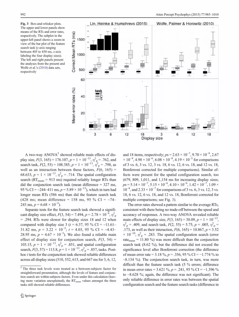
A two-way ANOVA5 showed reliable main effects of dis-play size, F(3, 165) = 176.107, p = 1 × 10−13, η2p = .762, andsearch task, F(2, 55) = 108.385, p = 1 × 10−13, η2p = .798, aswell as an interaction between these factors, F(6, 165) =68.633, p = 1 × 10−13, η2p = .714. The spatial configurationsearch (RTmean = 913 ms) required reliably longer RTs thandid the conjunction search task (mean difference = 327 ms,95 % CI = ~244–411 ms, p = 5.89 × 10−13), which in turn hadlonger mean RTs (586 ms) than did the feature search task(428 ms; mean difference = 158 ms, 95 % CI = ~74–243 ms, p = 6.68 × 10−5).

Separate tests for the feature search task showed a signifi-cant display size effect, F(3, 54) = 7.494, p = 2.78 × 10−4, η2p= .294. RTs were slower for display sizes 18 and 12 whencompared with display size 3 (t = 6.37, 95 % CI = ~11.61–31.82 ms, p = 3.22 × 10−5; t = 4.03, 95 % CI = ~4.43–28.95 ms, p = 4.67 × 10−3). We also found a reliable maineffect of display size for conjunction search, F(3, 54) =103.15, p = 1 × 10−13, η2p = .851, and spatial configurationsearch, F(3, 57) = 113.8, p = 1 × 10−13, η2p = .857, tasks. Post-hoc t tests for the conjunction task showed reliable differencesacross all display sizes (510, 552, 615, and 667 ms for 3, 6, 12,

and 18 items, respectively; ps = 2.63 × 10−7, 9.70 × 10−9, 2.67× 10−9, 4.98 × 10−6, 6.08 × 10−8, 4.19 × 10−5 for comparisonsof 3 vs. 6, 3 vs. 12, 3 vs. 18, 6 vs. 12, 6 vs. 18, and 12 vs. 18,Bonferroni corrected for multiple comparisons). Similar ef-fects were present for the spatial configuration search, too(679, 809, 1,011, and 1,154 ms for increasing display sizes;ps = 5.14 × 10−7, 5.15 × 10−9, 4.10 × 10−9, 1.42 × 10−7, 1.09 ×10−8, and 2.33 × 10−7 for comparisons of 3 vs. 6, 3 vs. 12, 3 vs.18, 6 vs. 12, 6 vs. 18, and 12 vs. 18, Bonferroni corrected formultiple comparisons; see Fig. 3).

The error rates showed a pattern similar to the average RTs,consistent with there being no trade-off between the speed andaccuracy of responses. A two-way ANOVA revealed reliablemain effects of display size, F(3, 165) = 38.09, p = 1 × 10−13,η2p = .409, and search task, F(2, 55) = 5.75, p = .005, η2p =.173, as well as their interaction, F(6, 165) = 10.867, p = 3.52× 10−10, η2p = .283. The spatial configuration search (errorratemean = 11.80 %) was more difficult than the conjunctionsearch task (8.62 %), but the difference did not exceed thesignificance level after Bonferroni correction (the differenceof mean error rate = 3.18 %, p = .356, 95 % CI = −1.774 % to~8.134 %). The conjunction search task, in turn, was moredifficult than the feature search task (5 % errors; differencein mean error rates = 3.621 %, p = .241, 95 % CI = −1.396 %to ~8.628 %; again, the difference was not significant). Theonly reliable difference in error rates was between the spatialconfiguration search and the feature search tasks (difference in

5 The three task levels were treated as a between-subjects factor forstraightforward presentation, although the levels of feature and conjunc-tion search are within-subjects factors. Even under this calculation (leav-ing more variation unexplained), the RTmean values amongst the threetasks still showed reliable differences.

Fig. 3 Box-and-whisker plots.The upper and lower panels showmeans of the RTs and error rates,respectively. The subplot in theupper-left panel shows a zoom-inview of the bar plot of the featuresearch task (y-axis rangingbetween 405 to 450 ms, x-axislabeling the four display sizes).The left and right panels presentthe analyses from the present andWolfe et al.’s (2010) data sets,respectively

992 Atten Percept Psychophys (2015) 77:985–1010

mean error rates = 6.801 %, p = .004, 95 % CI = 1.847 % to~11.755 %).

For the feature search, the effect of display size was notreliable, F(3, 54) = 1.517, p = .221, η2p = .078, whereas therewas a reliable effect of display size for both the conjunctionsearch task, F(3, 54) = 6.075, p = .001, η2p = .252, and thespatial configuration task, F(3, 57) = 41.426, p = 1.24 × 10−13,η2p = .686 (lower panel in Fig. 3). Post-hoc t tests indicatedthat in the conjunction search task, participants committedmore errors at display size 18 (13.05 %) than at display sizes12 (8.84 %; p = .028) and 6 (6.79 %; p = .043, Bonferronicorrected for multiple comparisons). In the spatial configura-tion search, there were differences across all display sizepairings except for 3 versus 6 (p = .161; ps = 5.90 × 10−5,9.85 × 10−6, 3.58 × 10−4, 6.80 × 10−6, and 1.21 × 10−5 for 3 vs.12, 3 vs. 18, 6 vs. 12, 6 vs. 18, and 12 vs. 18, Bonferronicorrected for multiple comparisons).

Error analysis

To test whether the shape change in an RT distribution wasdue to an increase of miss errors (Wolfe et al., 2010), we alsoanalyzed two types of errors: misses (i.e., participants pressedthe “absent” key in target-present trials) and false alarms (i.e.,participants pressed the “present” key in target-absent trials).

A two-way ANOVA on miss error rates showed reliablemain effects of display size, F(3, 165) = 38.08, p = 1 × 10−13,η2p = .409, and search task, F(2, 55) = 5.75, p = .005, η2p =

.173, as well as an interaction between these factors, F(6, 165)= 10.85, p = 3.62 × 10−10, η2p = .283. Both the spatial config-uration, F(3, 57) = 41.37, p = 1.25 × 10−13, η2p = .685, andconjunction search, F(3, 54) = 6.08, p = .001, η2p = .253, tasksshowed increasing miss errors as the display size increased,but the feature search task did not, F(3, 54) = 1.52, p = .221,η2p = .078. False alarms showed only a display size effect,F(3, 165) = 3.94, p = .010, η2p = .067. The reliable effect offalse alarm errors was observed in both feature search, F(3,54) = 2.81, p = .048, η2p = .135, and conjunction search, F(3,54) = 2.96, p = .040, η2p = .141, but not in spatial configura-tion search, F(3, 57) = 1.14, p = .340, η2p = .057 (Fig. 4).

Distributional analysis

Figure 3 also shows the distributions of the means of RTs anderror rates across the display sizes and tasks. Three noticeablecharacteristics are evident. First, performance in the featuresearch task changed little across the display sizes. Second, inthe two inefficient search tasks (conjunction and spatial con-figuration), increases in the display size not only delayed cen-tral RTs within the distribution (i.e., the estimates that medianand mean results aim to capture), but also shifted the entireresponse distribution. Third, the increases in task difficultyaffected not only central RTs, but also the variability of thedistribution. There were also some differences between theconjunction and spatial configuration tasks. The widely dis-tributed RTs for the spatial configuration task elongated the

Fig. 4 Mean rates of miss andfalse alarm errors. The error barsshow one standard error of themean. The y-axis showspercentage of errors. “F,” “C,”and “S” stand for feature,conjunction, and spatialconfiguration searches

Atten Percept Psychophys (2015) 77:985–1010 993

central measures of performance as well as the long-latencyresponses. Notably, the difference between the effects of thedifferent display sizes at the long end of the response distri-bution was exacerbated for the spatial configuration searchtask.

The box-and-whisker plot for error rates showed a similarpattern across the display sizes to the plot for the mean RTdata, although the effects were relatively modest inmagnitude.

Figure 5 shows the RT distributions at the differentdisplay sizes and search tasks. The distributions wereconstructed on the basis of the mean RTs (Nfeat andNconj = 19, Nspat = 20; 464 data points). The featuresearch showed a leptokurtic distribution, and thequantile–quantile plots indicated clear deviations at bothends of the distributions. The conjunction and spatialconfiguration search tasks at the small display sizes,however, showed only moderate signs of violation ofthe normality assumption, though at the large displaysizes, the distributions were platykurtic (flat) and thelong-latency RTs showed signs of deviation from a nor-mal distribution.

Figure 6 shows RT distributions and quantile–quantile plots. The distributions were constructed onthe basis of the trial RTs (43,485 data points). Eachdensity line represents the data from one participant.Evidently, the normality assumption was untenable

across all of the conditions. All subplots showed thatthe data clearly deviated from the theoretical normallines. It is also apparent that individual differencesplayed a more important role for the conjunction andspatial configuration tasks than for the feature task,judging by the diversity of the density lines in thetwo difficult search tasks.

Figure 7 shows the empirical cumulative distribu-tions, drawn on the basis of trial RTs (43,485 and109,036 data points in our and Wolfe et al.’s, 2010,data sets, respectively). The contrasting RTs across thedisplay sizes confirm Wagenmakers and Brown’s (2007)analysis that, in inefficient relative to efficient searchtasks, the RT standard deviation and RT mean play cru-cial roles in describing visual search performance.Specifically, the elongated cumulative distributions sug-gest that the more items are present, the more likely anobserver is to produce a response that falls in the righttail of the RT distribution. This observation again cau-tions us against a reliance solely on using measurementsof the central location when investigating visual searchperformance.

Contrasts with prior data

We compared our data with those of Wolfe et al. (2010). Acomparison of the mean RT and error rates indicated similar

Fig. 5 Mean RT distributions.The subplots within each panelare quantile–quantile (Q–Q)normalized plots showingdeviations of the data from thetheoretical normal distribution.The Q–Q normalized plotscompare RT means [y-axis label,“RT (ms)”] with normalized zscores [x-axis label, “Z-score”]. F,C, and S stand for feature,conjunction, and spatialconfiguration tasks, and P and Aare target-present and -absent trials, respectively

994 Atten Percept Psychophys (2015) 77:985–1010

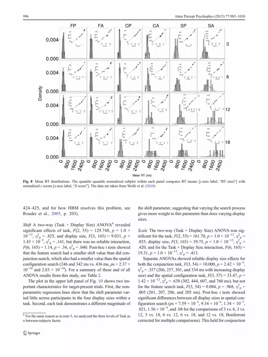
patterns across the studies (see Fig. 3), as is also suggested bythe cumulative density and RT plots shown in Figs. 7 and 8.

With only a small number of participants, it is difficult torule out the normality assumption when examining the mean

RTs (see the subplots in Fig. 8), but the data for the trial RTsreveal a skewed distribution (Fig. 9).

HBM estimates

In this section, we first present each parameter separate-ly for the respective ANOVA results, and compare thedata for the three search tasks at the different displaysizes, modeled by HBM. Next, we describe a nonpara-metric bootstrap regression to assess the relationship be-tween display size and the difficulty of the search task.The analysis focused on target-present trials. We usedthe deviance information criterion (DIC) to evaluateeach function’s fit to the data (see Table 1). In general,the smaller the DIC, the better the fit (Lunn, Jackson,Best, Thomas, & Spiegelhalter, 2013). Although thelognormal and Wald functions showed the smallestDICs, the DICs across the four fitted functions wereclose. Moreover, the diagnostics of the gamma HBMsuggests that its posterior distributions did not converge.Excluding the nonconverged gamma function, we arbi-trarily report estimates from the Weibull HBM, giventhat prior work has shown that this function providesa highly robust account, not strongly moderated bynoise in the data (for a specific pathology of theWeibull function, see Rouder & Speckman, 2004, pp.

Fig. 6 Trial RT distributions. Thequantile–quantile normalizedsubplot within each panelcompares trial RTs [y-axis label,“RT (ms)”] with normalized zscores [x-axis label, “Z-score”]

Fig. 7 Empirical cumulative RT density curves, drawn on the basis of thetrial RTs. The areas within each envelope represent the differencesbetween target-present and target-absent trials for each task. The twodashed lines show the positions of the 50 % and 95 % cumulative densi-ties. Long latencies (right border of envelopes) were consistently ob-served on target absent trials

Atten Percept Psychophys (2015) 77:985–1010 995

424–425, and for how HBM resolves this problem, seeRouder et al., 2005, p. 203).

Shift A two-way (Task × Display Size) ANOVA6 revealedsignificant effects of task, F(2, 55) = 129.748, p = 1.0 ×10−13, η2p = .825, and display size, F(3, 165) = 9.031, p =1.43 × 10−5, η2p = .141, but there was no reliable interaction,F(6, 165) = 1.14, p = .34, η2p = .040. Post-hoc t tests showedthat the feature search had a smaller shift value than did con-junction search, which also had a smaller value than the spatialconfiguration search (246 and 342 ms vs. 436 ms, ps = 2.37 ×10−10 and 2.83 × 10−10). For a summary of these and of allANOVA results from this study, see Table 2.

The plot in the upper left panel of Fig. 10 shows two im-portant characteristics for target-present trials. First, the non-parametric regression lines show that the shift parameter var-ied little across participants in the four display sizes within atask. Second, each task demonstrates a different magnitude of

the shift parameter, suggesting that varying the search processgives more weight to this parameter than does varying displaysizes.

Scale The two-way (Task × Display Size) ANOVA was sig-nificant for the task, F(2, 55) = 161.70, p = 1.0 × 10−13, η2p =.855, display size, F(3, 165) = 39.75, p = 1.0 × 10−13, η2p =.420, and for the Task × Display Size interaction, F(6, 165) =19.31, p = 1.0 × 10−13, η2p = .413.

Separate ANOVAs showed reliable display size effects forboth the conjunction task, F(3, 54) = 10.000, p = 2.42 × 10−5,η2p = .357 (206, 257, 301, and 334 ms with increasing displaysize) and the spatial configuration task, F(3, 57) = 33.47, p =1.42 × 10−12, η2p = .638 (302, 444, 607, and 760 ms), but notfor the feature search task, F(3, 54) = 0.084, p = .968, η2p =.005 (201, 207, 206, and 205 ms). Post-hoc t tests showedsignificant differences between all display sizes in spatial con-figuration search (ps = 7.59 × 10−3, 9.34 × 10−6, 1.34 × 10−7,.021, 1.56 × 10−4, and .04 for the comparisons of 3 vs. 6, 3 vs.12, 3 vs. 18, 6 vs. 12, 6 vs. 18, and 12 vs. 18; Bonferronicorrected for multiple comparisons). This held for conjunction

6 For the same reason as in note 5, we analyzed the three levels of Task asa between-subjects factor.

Fig. 8 Mean RT distributions. The quantile–quantile normalized subplot within each panel compares RT means [y-axis label, “RT (ms)”] withnormalized z scores [x-axis label, “Z-score”]. The data are taken from Wolfe et al. (2010)

996 Atten Percept Psychophys (2015) 77:985–1010

search only for the 3 versus 12, and 3 versus 18 comparisons(ps = .001, Bonferroni corrected for multiple comparisons).No significant differences were observed in feature search.

The lower left panel of Fig. 10 shows two importantcharacteristics. First, the regression lines indicate in-creasing variability (i.e., decreasing ribbon density) asthe display sizes increase for conjunction and spatialconfiguration search, but not for feature search.Second, the display size effect only becomes noticeable

for the inefficient search tasks, in line with the RTmean results.

Shape The two-way (Task × Display Size) ANOVA re-vealed significant effects of task, F(2, 55) = 23.50, p =4.21 × 10−8, η2p = .461, and marginally significant re-sults for display size, F(3, 165) = 2.44, p = .067, η2p =.042, and their interaction, F(6, 165) = 3.45, p = .003,η2p = .111.

Separate ANOVAs showed reliable display size effectsfor both conjunction search (1,496, 1,731, 1,695, and 1,702 with increasing display size), F(3, 54) = 4.21, p =.009, η2p = .190, and spatial configuration search (1,573,1,541, 1,397, and 1,529), F(3, 57) = 4.45, p = .007, η2p =.190, but not for feature search (1,702, 1,819, 1,976, and1,850), F(3, 54) = 2.13, p = .106, η2p = .106. Post-hoc ttests showed significant display size differences for 3 ver-sus 6, 3 versus 12, and 3 versus 18 items, ps = .022,.018, and .009, in the conjunction search. In the spatialconfiguration search, the display size differences were ob-served at 3 versus 12, 6 versus 12, and 12 versus 18

Fig. 9 Trial RT distributions. The quantile–quantile normalized subplot within each panel compares trial RTs [y-axis label, “RT (ms)”] with normalized zscores [x-axis label, “Z-score”]. The data are taken from Wolfe et al. (2010)

Table 1 Deviance information criteria of the four fitted functions

Present Study Wolfe et al. (2010)

Gamma 385,348,342 975,871,147

Lognormal 385,348,002 975,870,279

Wald 385,348,026 975,870,358

Weibull 385,348,139 975,871,078

The criteria are averaged across target-absent and -present trials, tasks,and display sizes.

Atten Percept Psychophys (2015) 77:985–1010 997

items, ps = .013, .047, and .003 (Bonferroni corrected formultiple comparisons).

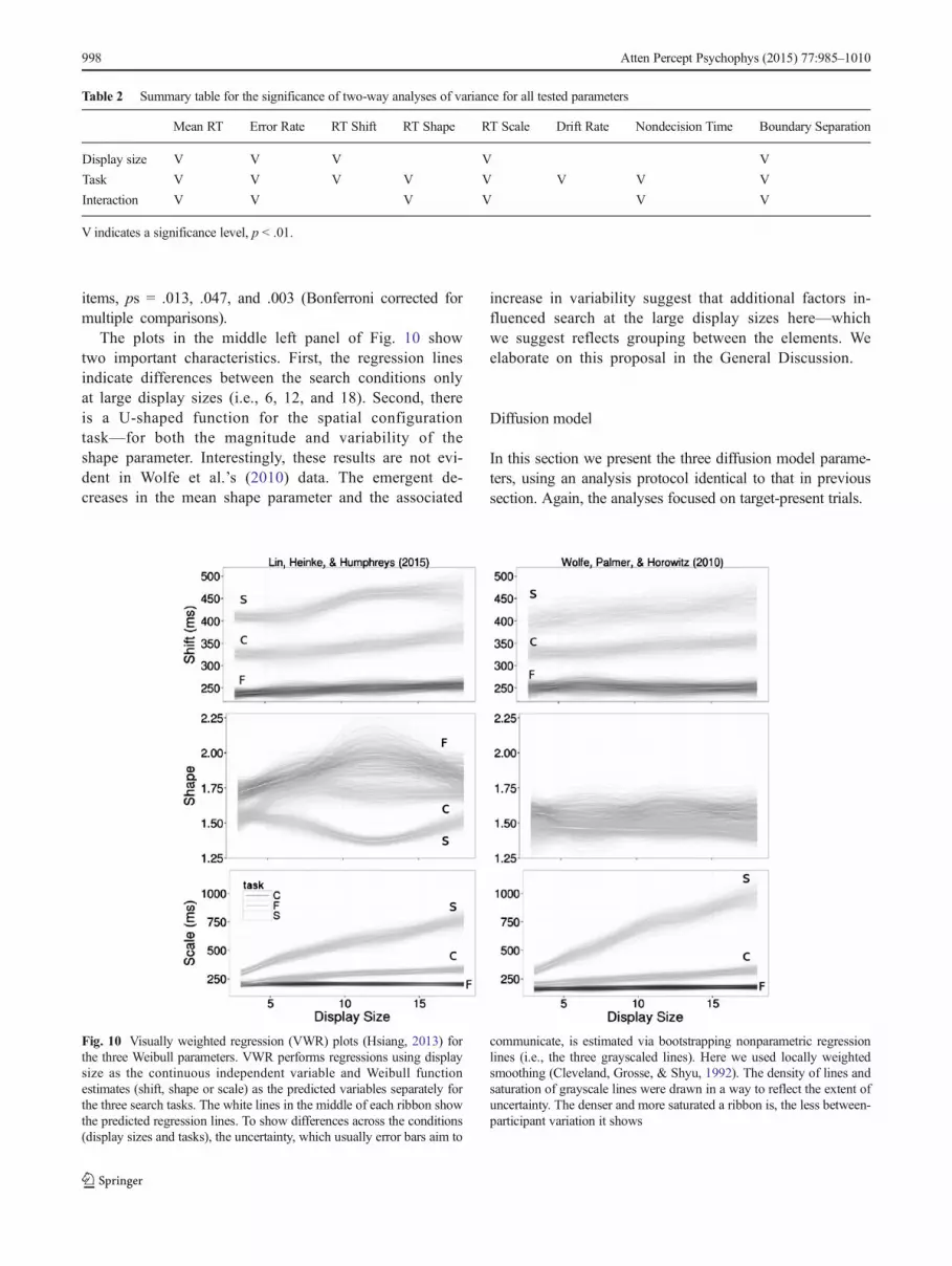
The plots in the middle left panel of Fig. 10 showtwo important characteristics. First, the regression linesindicate differences between the search conditions onlyat large display sizes (i.e., 6, 12, and 18). Second, thereis a U-shaped function for the spatial configurationtask—for both the magnitude and variability of theshape parameter. Interestingly, these results are not evi-dent in Wolfe et al.’s (2010) data. The emergent de-creases in the mean shape parameter and the associated

increase in variability suggest that additional factors in-fluenced search at the large display sizes here—whichwe suggest reflects grouping between the elements. Weelaborate on this proposal in the General Discussion.

Diffusion model

In this section we present the three diffusion model parame-ters, using an analysis protocol identical to that in previoussection. Again, the analyses focused on target-present trials.

Table 2 Summary table for the significance of two-way analyses of variance for all tested parameters

Mean RT Error Rate RT Shift RT Shape RT Scale Drift Rate Nondecision Time Boundary Separation

Display size V V V V V

Task V V V V V V V V

Interaction V V V V V V

V indicates a significance level, p < .01.

Fig. 10 Visually weighted regression (VWR) plots (Hsiang, 2013) forthe three Weibull parameters. VWR performs regressions using displaysize as the continuous independent variable and Weibull functionestimates (shift, shape or scale) as the predicted variables separately forthe three search tasks. The white lines in the middle of each ribbon showthe predicted regression lines. To show differences across the conditions(display sizes and tasks), the uncertainty, which usually error bars aim to

communicate, is estimated via bootstrapping nonparametric regressionlines (i.e., the three grayscaled lines). Here we used locally weightedsmoothing (Cleveland, Grosse, & Shyu, 1992). The density of lines andsaturation of grayscale lines were drawn in a way to reflect the extent ofuncertainty. The denser and more saturated a ribbon is, the less between-participant variation it shows

998 Atten Percept Psychophys (2015) 77:985–1010

Drift rate The two-way (Task × Display Size) ANOVA re-vealed a significant effect of task, F(2, 55) = 9.47, p = 2.92× 10−4, η2p = .256, but not of display size, F(3, 165) = 0.472, p= .703, η2p = .009, and no interaction, F(6, 165) = 1.27, p =.28, η2p = .044. Post-hoc t tests showed that the feature search(0.323) drifted faster than did the conjunction search (0.265;marginally significant, p = .057, 95 % CI = −0.117 to .001)and the spatial configuration search (0.220; p = 1.81 × 10−4,95 % CI = 0.044 to 0.161). No difference was found betweenthe conjunction and spatial configuration searches.

The drift rate, shown in the upper left panel in Fig. 11,manifests two critical characteristics. First, for both the featureand conjunction search tasks, the drift rate evolves at a con-stant rate across the display sizes. The second noticeable char-acteristic is a clear separation of the drift rates across the threetasks, suggesting differences in the rates at which sensoryevidence accumulates in the different tasks. There is also atendency for the drift rate to rise at the large display size inthe spatial configuration task (Fig. 11), suggesting that anemergent factor, such as the grouping of homogeneousdistractor elements, increased the drift rate—though the vari-ability across observers suggests that this was not universallythe case for all participants. This was not evident in target-absent trials.7 This upward trend was also not present in thedata of Wolfe et al. (2010).

Nondecision time The two-way (Task × Display Size)ANOVAwas significant for the main effect of task, F(2, 55)= 5.64, p = .006, η2p = .170, and the interaction, F(6, 165) =4.16, p = .001, η2p = .131. Post-hoc t tests showed that spatialconfiguration search (79 ms) was associated with a longernondecision time than were feature search (57 ms, p = .008,95%CI = 4.53 to 38.1ms) and conjunction search (61 ms, p =.038, 95 % CI = 0.707 to 34.2 ms). We observed reliabledisplay size effects for the spatial configuration task, F(3,57) = 6.886, p = 4.89 × 10−4, η2p = .266 (60.59, 80.54,89.50, and 84.23 ms with increasing display size), but notfor feature or conjunction search tasks.

Boundary separation The two-way (Task × Display Size)ANOVA revealed significant effects of the task, F(2, 55) =31.75, p = 6.81 × 10−10, η2p = .536, and the display size, F(3,165) = 7.6, p = 8.61 × 10−5, η2p = .121, as well as a Task ×Display Size interaction,F(6, 165) = 4.76, p = 1.69 × 10−4, η2p= .147. The value of the boundary separation for featuresearch (0.111) was smaller than that for spatial configurationsearch (0.192; p = 1.01 × 10−9, 95 % CI = 0.055 to 0.107) andwas not different from that found for conjunction search(0.132). The conjunction search task also demonstrateda reliable difference from the spatial configuration con-dition (p = 1.49 × 10−6, 95 % CI = 0.034 to 0.086).Separate ANOVAs showed reliable display size effectsfor the spatial configuration search (0.148, 0.170, 0.201,and 0.249 for 3, 6, 12, and 18 items, respectively), F(3,

Fig. 11 Visually weightedregression plot for the EZ2diffusion model parameters

7 See https://github.com/yxlin/HBM-Approach-Visual-Search for thetarget-absent trial data.

Atten Percept Psychophys (2015) 77:985–1010 999

57) = 6.73, p = .001, η2p = .262, but not for the featureor conjunction searches.

General discussion

In this study, we applied an integrated approach to themodeling of visual search data. We examined the datanot only using standard aggregation approaches, but al-so using distributional approaches to extract cognitive-related parameters from the trial RTs. This approachallowed us to reveal the possible accounts of the threedistributional parameters—shift, shape, and scale—byassociating them with the nondecision time, drift rate,and boundary separation estimated from the diffusionmodel. Our study goes farther than most previous ones(Balota & Yap, 2011; Heathcote et al., 1991; Sui &Humphreys, 2013; Tse & Altarriba, 2012) that have ap-plied distributional analyses to RT data. We used con-ventional distributional analyses to examine empiricalRT distributions, and the associated parameters werecomplemented with Bayesian-based hierarchical model-ing to optimize the estimates. Moreover, we examinedthose distributional parameters against a plausible com-putational model—the EZ2 diffusion model—to link thedistributional parameters to underlying psychologicalprocesses.

Replicating many previous findings in the search literature,our data showed efficient search for feature targets and ineffi-cient search when targets could only be distinguished fromnontargets by conjoining multiple features (shape and color,or shape only; see Chelazzi, 1999, and Chun & Wolfe, 2001,for reviews). The display size effect present in feature search(415, 426, 432, and 437 ms) suggests some limitations onselecting feature targets, but the analyses based on mean RTsdid not differentiate whether the effect (η2p = .294) was due topostselection reporting (Duncan, 1985; Riddoch &Humphreys, 1987) or to an involvement of focal attention infeature search. This question was addressed by examining theestimates from HBM together with those from the EZ2 diffu-sion model. The lack of display size effects for nondecisiontime suggests that the increasing trend in the mean RTs wasunlikely to be due to a delay in peripheral processes, such asmotor or early perceptual times. Neither drift rate showed areliable effect of the display size for feature search. The onlypossible difference was an unreliable display size effect (p =.106), together with an increase of variation in the shape pa-rameter at display size 18. This result appears to favor theexplanation of focal attention.

Though previous results have indicated that search is ofteninefficient for conjunction- and configuration-based stimuli,our findings indicated that spatial configuration search was

particularly difficult (Bricolo et al., 2002; Kwak et al., 1991;Woodman& Luck, 2003). This could reflect either a reductionin the guidance of search from spatial configuration, as com-pared with simple orientation and color information, or in thelength of time taken to identify each item after it had beenattended. Interestingly, although when compared with thestandard deviation of the conjunction search (9.68 ms), con-figuration search generally showed a larger value across par-ticipants (24.54 ms), the standard deviations within the con-figuration search decreased as the display sizes increased(35.17, 27.12, 15.38, and 20.49 ms). This last result suggeststhat high-density homogeneous configurations of distractorsdo facilitate search, a point that we return to below (Bergen &Julesz, 1983; Chelazzi, 1999; Duncan & Humphreys, 1989;Heinke & Backhaus, 2011; Heinke & Humphreys, 2003).

Methodological issues

The analyses of the mean RTs, however, did not alwaysaccord with the analyses of trial RTs. For example, thedensity plots of mean RTs (Fig. 5) suggest that the datawere distributed symmetrically, contrasting with thecommon notion that an RT density curve tends to bepositively distributed toward long latencies (Luce,1986). However, the analyses of the trial RTs (Fig. 6)revealed clearly skewed RT distributions. This was be-cause the procedure of determining a representative val-ue using a central location parameter (the mean, in thecase of our data) from each observer’s RT distributionfor a condition (individual curves in Fig. 6) is affectedgreatly by the weight of the slow RTs. The conditionsand observers that contribute the slow responses tend tomove the central location toward longer latencies withina distribution; hence, we observed more symmetricaland sub-Gaussian (i.e., flat) density curves for the meanRTs. Additionally, because the density curve for themean RTs is usually constructed by means of a biasedcentral-location parameter (with respect to a skewed RTdistribution), the nature of the RT distribution (e.g., ifthere are a majority of quick responses and a minorityof slow responses) is hidden by an unrepresentativecentral-location parameter. A solution has been proposedrecently of using some variants of distributional analy-ses (Balota & Yap, 2011; Bricolo et al., 2002;Heathcote et al., 1991), and these have been appliedto various cognitive tasks (Palmer et al., 2011; Sui &Humphreys, 2013; Tse & Altarriba, 2012; Wolfe et al.,2010). Essentially, the distributional approach constructsan empirical distribution by using the trial RTs fromeach individual in a condition and uses a plausible dis-tributional function (such as Weibull or ex-Gaussian) toextract distributional parameters, with the parameters be-ing averaged across participants and then compared

1000 Atten Percept Psychophys (2015) 77:985–1010

across the different conditions. This approach descrip-tively dissects an RT distribution into multiple compo-nents (e.g., mu, sigma, and tau), each potentiallyreflecting a contrasting psychological process (Balota& Yap, 2011). However, the link between the compo-nent and the underlying process can be elusive (Matzke& Wagenmakers, 2009) without directly modeling of theunderlying factors. We addressed this issue by contrast-ing the empirical data modeled by both a distributionalapproach (HBM) and a computational model (the EZ2diffusion model).

On top of the analyses of mean performance, the integra-tion of hierarchical Bayesian and EZ2 diffusion modelinghelped to throw new light on search. Following Rouder et al.(2005), HBM dissects an RT distribution into three parame-ters: shift, scale, and shape. The shift parameter has beenlinked to residual RTs, the scale parameter with the responserate, and the shape parameter with postattentive response se-lection (Wolfe, Võ, Evans, & Greene, 2011). The EZ2 diffu-sion model directly estimates three parameters: (1) the driftrate, reflecting the quality of the match between a memorytemplate and a search display (the goodness of match, inRatcliff & Smith’s, 2004, terms); (2) the boundary separation,reflecting the response criterion (Wagenmakers et al., 2007);and (3) the nondecision time, reflecting the time that an ob-server requires to encode stimuli and execute a motor re-sponse. This conceptualization can help articulate the correla-tion between the descriptive parameters from the RT distribu-tion and those estimated by the diffusion model. For example,the role of shift in a Weibull function is to directly set a min-imal threshold for responses and rule out the possibility ofnegative responses. This suggests an association between theRT shift and nondecision time parameters.

Model-based analysis

The EZ2 diffusion model and HBM results suggest that dis-tributional parameters reflect different aspects of search. First,the shift parameter varied across the search tasks and displaysizes, a pattern that was in line with our illustration and theideal analysis (see Fig. 1 and Appendix 2). This parameterreflects the psychological processes that evenly influence allranges of RTs. One of the diffusion processes likely to influ-ence the shift changes is the drift rate, which showed only amain effect of task. Since the drift rate aims to model the rateof information accumulation determined by the goodness ofmatch between the templates and search stimuli, the shift pa-rameter appears to result from a change in the quality of thememory match. This is a plausible account, because the threesearch tasks demand contrasting matching processes, from (i)feature search, which requires only preattentive parallel pro-cessing to extract just one simple salient feature, to (ii) con-junction search, in which two simple features must be bound

to facilitate a good match, to (iii) spatial configuration search,which demands both feature binding and coding the configu-ration of the features. The lack of an interaction with displaysize further supports our argument that the shift reflects factorsthat affect the entire RT distribution equally. The weak displaysize effect can be readily explained by the crowded layout thatwe used; it had not been observed [F(3, 75) = 0.016, p = .997]in Wolfe et al.’s (2010) data. This weak effect of the shiftparameter is further accounted for by our visually weightedplot in the drift rate parameter, showing a clear split of trendsand an increase of between-observer variation at the largedisplay size. Specifically, a subset of participants adopted astrategy similar to those of the participants in Wolfe and col-leagues’ (2010) study. These participants did not assemble asimilarity search unit, so the predicted drift rate decreased atlarge display sizes, whereas the other subset of participantsbenefited from the crowded homogeneous distractors, andthus increased drift rate at the large display sizes.

Another account for the strong task effect but the weakeffect of display size is that this pattern reflects a process suchas the recursive rejection of distractors, proposed byHumphreys and Müller (1993) in their SERR model of visualsearch (see also Heinke & Humphreys, 2005). Humphreysand Müller argued that search can reflect the grouping andthen recursive rejection of distractors. The process here mayreflect the strength of grouping rather than the number ofdistractors, since multiple distractors may be rejected togetherin a group—indeed, effects of the number of distractors maybe nonlinear, since grouping can increase at larger displaysizes. Grouping and group selection both reflect the similarityof targets and distractors and the similarity of the distractorsthemselves, and these two forms of similarity vary in oppositedirections in conjunction and spatial configuration search (rel-ative to a feature search condition such as the one employedhere, the two types of search respectively reflect weakerdistractor–distractor grouping and stronger target–distractorgrouping; see Duncan & Humphreys, 1989). If the processof distractor rejection is more difficult in conjunction and con-figuration search, as compared with feature search, then theeffects on a parameter will reflect this process, and this maynot vary directly with display size, as we observed.

In contrast to the shift parameter, the shape parametershowed a marginal effect of display size, a reliable effect oftask, and an interaction between these factors. The magnitudeof this parameter increased monotonically with the displaysize for the feature and conjunction searchers, but demonstrat-ed a U-shaped function for the spatial configuration search.This last result is consistent with a contribution from an emer-gent property of the larger configuration displays, such as thepresence of grouping between the multiple homogeneousdistractors leading to a change in perceptual grouping (seealso Levi, 2008, for a similar argument concerning visualcrowding). This change in the shape parameter in the large

Atten Percept Psychophys (2015) 77:985–1010 1001

display size of the spatial configuration task is in line with asudden increase of the drift rate standard deviation (0.080,0.050, 0.054, and 0.344 with increasing display size), suggest-ing either (1) a change in the quality of a match between thestimuli and the template or (2) a variable grouping unit(amongst different observers) affecting the recursive rejectionprocess.

In addition, we observed a general increase in the values ofthe shape parameter, from 1.73 at display size 3, to 1.86 atdisplay size 6, 2.05 at display size 12, and 1.96 at display size18, on target-absent trials in the spatial configuration task, F(3,57) = 6.13, p = .001, η2p = .244. The target-absent-inducedshape change in the spatial configuration task was also ob-served in Palmer et al.’s (2011) analysis. However, their datashowed no reliable shape change across display sizes fortarget-present trials (Palmer et al., 2011). Following Wolfeet al.’s (2010) suggestion, Palmer and colleagues speculatedthat the display size effect for the shape parameter might resultfrom the premature abandoning of search, a view that wassupported by Wolfe et al.’s (2010) data showing a high rateof miss errors in the spatial configuration task. The high rate ofmiss errors might reflect an observer prematurely deciding togive an “absent” response on a target-present trial. This would,in turn, reduce the overall number of slow responses, leadingto an RT distribution with low skewness. This indicates that inthe conditions with high miss errors, participants tended to seta low decision threshold for the “absent” response. The ten-dency might also appear in the target-absent trials, resulting incorrect rejections by luck, a result leading to RT distributionsin these trials with an increase in the shape parameter. We,applying a more sensitive method under the constraint of lim-ited trial numbers, showed reliable display size effects on theRTshape in the target-present trials of the spatial configurationand conjunction searches. Together with the miss error data,our data do indicate that a link between miss errors and theshape of the RT distribution is plausible. In addition to theexplanation of participants abandoning search prematurely(i.e., a dynamic changes of boundary separation), we proposeanother explanation: Relative to feature search, the factor thatchanges the RT shape in spatial configuration search is thegoodness of match between the search template and the searchdisplay (i.e., the drift rate changes). This implies that factorscontributing to change in different parts of an RT distributionwill result in its shape changing. As our simulation studyshows (see Appendix 2), doubling the shape parameter resultsin a decrease in boundary separation (in line with the misserror account) and an increase in the drift rate (in line withthe goodness-of-match account). The two diffusion parame-ters are likely the processes driving changes in the shape of theRT distribution.

Among the three Weibull parameters, the scale parametershowed the highest correlation with mean RTs (Pearson’s r =.78, p = 2.20 × 10−16), a result replicating Palmer et al.’s

(2011) analysis. The high correlation should not be surprising,considering that both the RT scale and the mean RTs capturechange in the central location of the RT distributions. Thescale parameter estimates an overall enhancement (or reduc-tion) of response latency as well as response variance, as dothe mean and variance of RTs (see the review inWagenmakers& Brown, 2007). Unlike the mean RTs, however, the scaleparameter in our data set was not sensitive to the display sizein the feature search task. A cross-examination with theboundary separation in the diffusion model appeared to indi-cate that the scale parameter might reflect the influence ofresponse criteria, with only the inefficient tasks showing adisplay size effect. This should not be taken as evidence indi-cating that the scale parameter is a direct index of the responsecriteria, however; rather, changes in the scale parameter are aconsequence of altering the response criteria. An observerwith a conservative criterion, for example, might show a gen-eral change in response latency and variance (the more reluc-tant one is to make a decision, the more variable a responsewill be), so the scale parameter reflects this change.

Distributional parameters reflect underlying processes

The RT distributional parameters have been posited, under theframework of the stage model of information processing, toreflect different aspects of peripheral and central processing.The shift parameter has been associated with the speed ofperipheral processes (i.e., the irreducible minimum responselatency; Dzhafarov, 1992), the scale parameter with the speedof executing central processes, and the shape and scale param-eters with the insertion of additional stages into central pro-cessing (Rouder et al., 2005).

Using benchmark paradigms of visual search (Wolfe et al.,2010), our data indicate that the shift parameter, instead ofreflecting the speed of peripheral processes, may be associatedwith the process of distractor rejection and the quality of thematch between a template and a search display. This is sup-ported by the analysis using the EZ2 diffusion model. As weargued previously, the shift parameter captures the factors thatinfluence the entire RT distribution equally. A possible situa-tion in which a peripheral process may result in a clear shiftchange is when the other two parameters are kept constant—that is, when no factor influences the decision-making processand when the shape of an RT distribution is unchanged. Wesuggest that the data better reflect a process such as the recur-sive rejection of grouped distractors and the quality of thematch to a target template, which, when accurate, contributesto the entire RT distribution.

Our results for the scale parameter are consistent with thoseof Rouder and colleagues (2005) in suggesting that this pa-rameter reflects the speed of execution in a central decision-making process. Since the execution speed closely links withthe decision boundaries and the initial state of sensory

1002 Atten Percept Psychophys (2015) 77:985–1010

information that an observer sets for a response trial, we ob-served similar patterns in the scale parameter, the boundaryseparation, and the nondecision time. The pattern in the non-decision times is readily accounted for by the fact that the EZ2diffusion model absorbs the parameter reflecting the initialstate of sensory evidence into the nondecision time. The dis-tance between the decision boundary and the initial state ofsensory evidence can then be taken as reflecting changes inthe response criteria, and hence altering the scale of an RTdistribution.

For the shape parameter, we observed an emergent effect ofperceptual grouping for the large display size in the spatialconfiguration search. This is in line with the drift rate data,in that the drift rate was slower for the spatial configurationsearch task than for the two simple search tasks, in both ourdata (0.323 and 0.265 vs. 0.220) and those of Wolfe et al.(2010; 0.341 and 0.299 vs. 0.203). In Palmer et al.’s (2011)analysis, no task effect was found in the shape parameter.Using HBM, we observed a significant task effect, F(2, 55)= 23.50, p = 4.21 × 10−8, η2p = .461, suggesting that theprevious result might reflect a lack of power. The observationsof shape invariance in Palmer et al.’s analysis could also beinterpreted in terms of a memory match account (Ratcliff &Rouder, 2000). This account presumes that, when the integrityof a memory match between the template and search items isstill intact, the evidence strength is strong enough to permit acorrect decision (Smith, Ratcliff, & Wolfgang, 2004; Smith &Sewell, 2013). Since in the previous study fewer participantswere recruited, and some might have found strategies throughwhich to conduct the difficult searches while still using thesame processing stages as in the feature search task, the shapeparameter reflected only a marginal effect.

Another possible factor that may explain the different find-ings for the shape parameter is illustrated by the visuallyweighted plot of drift rate. The visually weighted regressionlines indicate two groups of participants accumulating sensoryevidence at different rates, where only one homogeneousgroup appeared inWolfe et al.’s (2010) data. As our simulatedstudy showed (Appendix 2), the drift rate can also change theshape parameter. This suggests that some of our participantstook advantage of the crowded layout to facilitate search in thespatial configuration task, and some did not. This could nothappen in Wolfe et al.’s (2010) sparse layout, and likely alsocontributed to our significant finding for the shape parameteron target-present trials.

Limitation

The analytic approach that we adopted assumes that individ-ual RTs are generated by three-parameter probability func-tions. Our selection of the Weibull function was determined,on the one hand, by its probing three important aspects—theshift, scale, and shape—of an RT distribution, which differs

from what the ex-Gaussian function describes (mu, tau, andsigma). On the other hand, we selected the Weibull functionbecause it permits a reliable posterior distribution to converge,has broad application to memory as well as to visual search(Logan, 1992; see also Hsu&Chen, 2009), and also can applyto the hierarchical Bayesian framework (Rouder et al., 2005).

Conclusion

In conclusion, our study shows that an HBM-based distribu-tional analysis, complemented with the EZ2 diffusion model,can help to clarify the processes mediating visual search. Thedata indicate that different effects of search difficulty contrib-ute to performance, with the effects of the search conditionbeing distinct from those of display size in some cases (on thedrift rate and shift parameters), but not in others (e.g., effectson nondecision factors and on the separation of decisionboundaries). We have linked this dissociation to the involve-ment of distractor grouping and rejection (on the one hand)and to serial selection of the target and the setting of a responsecriterion (on the other). This approach goes beyond what canbe done using standard analyses based on mean RTs.

Appendix 1

HBM simulations

The stimulation study was performed to examine the estima-tion biases on three standard distributional parameters—mean, variance, and skewness—when various probabilityfunctions were fitted under different sample sizes per experi-mental condition and the true distributions generating the RTswere known. The study helped clarify whether the per-condition trial number was sufficient to allow reliable param-eter estimation using HBM. The conclusion from this simula-tion suggested that (1) no difference in results distinguishedHBM from maximum likelihood estimation (MLE) when thesample size was larger than 120; (2) HBM was better thanMLE at estimating variance when the sample size was small;and (3) the specification of equally plausible probability func-tions is crucial only when the function matches the true distri-bution that generated the RT data.

Through simulations8 we examined four scenarios, alterna-tively assuming that the true distribution followed a normal,an ex-Gaussian, a Wald, or a Weibull function (which adoptedCousineau, Brown, & Heathcote’s, 2004, parameter values).

8 We used R routines—rnorm, rexGAUS, rinvgauss, and rweibull3—togenerate those computer-simulated data.

Atten Percept Psychophys (2015) 77:985–1010 1003

Specifically, we used the parameter values listed in Table 3 ofCousineau et al.’s report to construct four true distributions,which in turn repeatedly generated randomly simulated RTs.The simulations generated 20 homogeneous participants; eachparticipant contributed RT observations for ten different sam-ple sizes, ranging from 20 to 470 with a step size of 50. Thesimulated data were then submitted separately to HBM and to

MLE to estimate the shift, scale, and shape parameters. Bothmethods assumed that RTs were random variables generatedby the Weibull function. Those parameters were then analyt-ically converted to the mean, variance, and skewness to eval-uate the performance of the two methods.

Figure 12 shows the absolute values of the differences be-tween the true values and the estimates at the mean, variance,and skewness of a distribution. In general, no differences wereobserved between the twomethods when estimating the mean.The only factor that improved the estimation was the per-condition sample size, F(9, 1520) = 64.46, p < .0001: Themore observations were in a condition, the higher wasthe precision of the estimate. The bias dropped rapidlywhen the trial number surpassed 100, from 17.59 ms at20 observations to 6.74 ms at 120 observations, and itdecreased at a slower rate when the trial size was over120 observations (on average, 5.4 ms). The specificationof the true distribution did not alter the precision ofmean estimation, F(3, 1520) = 1.912, p = .126, eventhough both estimation methods assume that a Weibullfunction accounted for the RT data.

In contrast, HBM demonstrated a clear advantage over theMLE method when recovering the variance, F(1, 1520) =9.345, p = .0023. Again, a large number of observations helpedto improve the fit, F(1, 1520) = 29.84, p < .0001. Importantly,HBM estimated the parameters better than MLE at the smallestsample size (N = 20), F(1, 152) = 6.907, p = .0095, though thedifference was gradually resolved when the observation num-bers exceeded 120, F(1, 152) = 0.936, p = .335 (i.e., the dashedline in Fig. 1). Misspecification of the underlying distributionresulted in different estimations of variance,F(3, 1520) = 7.635,p < .0001. Both methods needed a sample size larger than 170to resolve this issue (the dotted line in Fig. 12). Parameter

Fig. 12 Sample mean, variance, and skewness values, compared to thetrue values that generated the simulated data. “HBM” and “MLE” standfor the hierarchical Bayesian model and maximum likelihood estimates,respectively. The mean and variance are in scales of seconds and squaredseconds, respectively. The skewness was calculated by dividing the thirdmoment about the RT mean [m3 = (RT – RTmean)

3/N] by the cube of theRT standard deviation, which renders it dimensionless (Crawley, 2002).The three dashed lines are drawn at sample sizes of 120, 170, and 220 toshow critical changes in the three parameters with regard to the samplesizes

Fig. 13 The estimation of skewness. The figure traces the differencesbetween hierarchical Bayesian modeling (HBM) and maximum likeli-hood estimation (MLE) at different sample sizes in an experimentalcondition

Fig. 14 Goodness of fit of the empirical data against the Weibulldistribution, using the maximum likelihood estimation(MLE) andhierarchical Bayesian modeling (HBM) methods

1004 Atten Percept Psychophys (2015) 77:985–1010

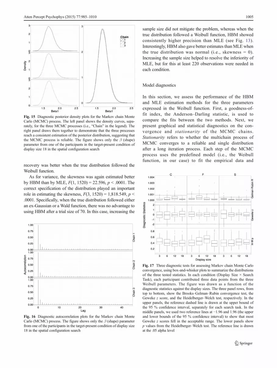
recovery was better when the true distribution followed theWeibull function.

As for variance, the skewness was again estimated betterby HBM than by MLE, F(1, 1520) = 22.596, p < .0001. Thecorrect specification of the distribution played an importantrole in estimating the skewness, F(3, 1520) = 1,818.549, p <.0001. Specifically, when the true distribution followed eitheran ex-Gaussian or a Wald function, there was no advantage tousing HBM after a trial size of 70. In this case, increasing the

sample size did not mitigate the problem, whereas when thetrue distribution followed a Weibull function, HBM showedconsistently higher precision than MLE (see Fig. 13).Interestingly, HBM also gave better estimates thanMLEwhenthe true distribution was normal (i.e., skewness = 0).Increasing the sample size helped to resolve the inferiority ofMLE, but for this at least 220 observations were needed ineach condition.

Model diagnostics

In this section, we assess the performance of the HBMand MLE estimation methods for the three parametersexpressed in the Weibull function. First, a goodness-of-fit index, the Anderson–Darling statistic, is used tocompare the fits between the two methods. Next, wepresent graphical and statistical diagnostics on the con-vergence and stationarity of the MCMC chains.Stationarity refers to whether the multichain process ofMCMC converges to a reliable and single distributionafter a long iteration process. Each step of the MCMCprocess uses the predefined model (i.e., the Weibullfunction, in our case) to fit the empirical data and

Fig. 15 Diagnostic posterior density plots for the Markov chain MonteCarlo (MCMC) process. The left panel shows the density curves, sepa-rately, for the three MCMC processes (i.e., “Chain” in the legend). Theright panel draws them together to demonstrate that the three processesreach a consistent estimation of the posterior distribution, suggesting thatthe MCMC process is reliable. The figure shows only the β (shape)parameter from one of the participants in the target-present condition ofdisplay size 18 in the spatial configuration search

Fig. 16 Diagnostic autocorrelation plots for the Markov chain MonteCarlo (MCMC) process. The figure shows only the β (shape) parameterfrom one of the participants in the target-present condition of display size18 in the spatial configuration search

Fig. 17 Three diagnostic tests for assessing Markov chain Monte Carloconvergence, using box-and-whisker plots to summarize the distributionsof the three tested statistics. In each condition (Display Size × SearchTask), each participant contributed three data points from the threeWeibull parameters. The figure was drawn as a function of thediagnostic statistics against the display sizes. The three panel rows, fromtop to bottom, show the Brooks–Gelman–Rubin convergence test, theGeweke z score, and the Heidelberger–Welch test, respectively. In theupper panels, the reference dashed line is drawn at the upper bound ofthe 95 % confidence interval, separately for each search task. In themiddle panels, we used two reference lines at −1.96 and 1.96 (the upperand lower bounds of the 95 % confidence interval) to show that mostGeweke z scores fell in the acceptable range. The lower panels showp values from the Heidelberger–Welch test. The reference line is drawnat the .05 alpha level

Atten Percept Psychophys (2015) 77:985–1010 1005

predict a posterior distribution. The posterior distribu-tion is then used as a prior distribution in the next stepto fit a new posterior distribution. This process iteratesitself until the predefined number of iterations (105,000in our setting). The final posterior distribution was thepredicted distribution presumed to be the true distribu-tion underlying an RT distribution in the visual searchparadigm that we examined. We ran three separate in-dependent MCMC processes (i.e., three chains) to testwhether all three converged to an identical final poste-rior distribution. If this was so, it would indicate thatour hierarchical Bayesian setting and the Weibull func-tion provided an appropriate approximation of an RTdistribution. A nonconvergent MCMC process wouldnot provide a reliable prediction for the final posteriordistribution. That is, it would predict, even after a longiteration process, different distributions accounting forthe empirical data.

Goodness of fit Because RT distributions are formed by acontinuous rather than a discrete random variable, we usedthe Anderson–Darling statistic, rather than chi-square, as theindex of goodness of fit. Figure 14 shows that there were fewdifferences between the MLE and HBM fits: Both methodsperformed similarly and improved their fits as the display sizeincreased.

Bayesian model diagnosis In this section, we examine wheth-er the estimated parameters converged to a stationary posteriordistribution and whether the setting for conducting MCMCsampling was appropriate for permitting reliable inferences.

Figures 15 and 16 shows one of the examples of thediagnostic plots, indicating the convergence of β (i.e.,the shape parameter), which was estimated from one ofthe participants performing the spatial configurationsearch at display size 18 in the target-present condition.The figures are the posterior density curve and the au-tocorrelation plot. We ran three Markov chains in par-allel to approach a stationary posterior distribution, sothree sets of parallel data represent the three processes.Three MCMC chains mixed quickly to a limited rangeafter the iteration process began (after 5,000 burn-initerations), suggesting that the posterior distributionreached a reliable stationary point.9 This impression issupported by the posterior density distributions(Fig. 15), showing that all three chains predict overlap-ping distributions with very similar shapes and disper-sions, consistent with the three chains predicting identi-cal posterior distributions. The autocorrelation plots(Fig. 16) showed that the MCMC sampling interval (inour case, the computer program took one sample every

9 A nonstationary mix will manifest as three clearly separated lines.

Fig. 18 Figure showing howchanges in the distributionalparameters may alter theparameters estimated by the EZ2diffusion model. Ter, a, and vstand for the nondecision time,boundary separation, and driftrate, respectively

1006 Atten Percept Psychophys (2015) 77:985–1010

four iterations) is appropriate to reduce the interiterationcorrelation rapidly within first 50 iterations (after thefirst 5,000 samples have been discarded).

The information from the graphical diagnoses is com-patible with the nonparametric statistical tests. Figure 17presents the graphical summary of the nonparametrictests for the stationarity across all the conditions andparticipants. The upper panels show the Brooks–Gelman–Rubin (BGR; Brooks & Gelman, 1998) shrinkfactor. The recommended BGR upper limit is 1.1(Gelman, 2004; Gelman & Hill, 2007), and values be-low it are deemed acceptable. We drew the referenceline at the grand average 95 % confidence interval toallow a clear inspection of the distribution for the sta-tistics. Very few BGR diagnostics exceeded the grandaverage of 95 % confidence interval. Although a fewvalues fall outside the upper limit of the box-and-whisker plots, they are nevertheless all within the rec-ommended upper limit. The BGR shrink factor providesno evidence of an unstable mixing of the three chains,confirming the observations from the trace plots.

The middle panels show the Geweke z score. This testexamines the stationarity of the posterior distribution. A zscore exceeding ±1.96 is considered problematic. Only afew cases at display size 6 in the conjunction search and atdisplay size 3 in the spatial configuration search exceeded thetwo reference lines, drawn at Z = ±1.96. In general, the distri-bution of the Geweke z is compatible with the stationarityassumption that we have observed in the posterior densityplots. In other words, the posterior distribution estimated fromthe three separate chains converged to an identicaldistribution.

The lower panels show the distribution of the p values fromHeidelberger and Welch’s test. The reference line was drawnat a .05 p value. The figure complements the observationsfound both in the graphical diagnostics and the Geweke z test.None of the p values exceeded .05 levels. In summary, wefound, from both graphical diagnoses and nonparametric tests,no obvious evidence, in all estimated parameters across allparticipants and conditions, against either the hypothesis ofthe stationarity of the posterior distributions, the ill-mixedMarkov chains, or an unreliable convergence.

Fig. 19 The figure compares the Bayesian deviance information criteria for the fitted three-parameter probability functions across the data sets, searchtasks, target types, and display sizes. “L” and “W” stand for our and Wolfe et al. (2010) data sets

Atten Percept Psychophys (2015) 77:985–1010 1007

Appendix 2: EZ2 diffusion model simulations

The stimulation study was undertaken to examine how theparameters estimated from the EZ2 diffusion model correlatewith the Weibull parameters in a simple, well-controlled situ-ation. We performed three case studies in which we changedonly one of the Weibull parameters. Note that the three distri-butional parameters jointly determine the general shape of adistribution. Thus, a change in the drift rate may alter one ormore of the Weibull parameters. In the three studies, we dou-bled, respectively, the shift, the scale, and the shape parame-ters in a Weibull function and simulated 200 RTs from 20homogeneous observers.

The data were than submitted to the EZ2 model toestimate the drift rate, boundary separation, and nonde-cision time. The results indicated that, first, doublingthe shift parameter resulted in a near two-fold increasein nondecision time (416 vs. 827 ms), a small increasein drift rate (0.012 vs. 0.013), and a small decrease inboundary separation (4.89 vs. 4.57). Second, doublingthe scale parameter resulted in a decrease in drift rate(0.013 vs. 0.009), an increase in boundary separation(4.70 vs. 6.57), and a 10-ms increase in the nondecisiontime (407 vs. 417 ms). Finally, doubling the shape pa-rameter resulted in an increase in drift rate (0.013 vs.0.018), a decrease in boundary separation (4.57 vs.3.39), and again, a small increase in the nondecisiontime (410 vs. 507), although this increase was relativelylarger than that from doubling the scale parameter.Figure 18 shows a comparison across the three casestudies.

Appendix 3: Why use the Weibull function?

The Weibull probability function is one of the manyplausible functions that can accommodate positivelyskewed RT distributions. We chose it to describe theRT distributions because of its parametric characteris-tics, permitting us to describe the shape of an RT dis-tribution in an intuitive way. Nevertheless, there areother alternatives, such as the gamma, lognormal, andWald functions. All of them are capable of accommo-dating skewed RT distributions and provide similar de-scriptive parameters. Here, we delineate our reasons tofit the HBM Weibull function to our RT data.

The first reason is that the Weibull function is able to pro-vide a concise way to summarize the shape of an RT distribu-tion. As is described in the main text and illustrated in Fig. 1,changes in the three parameters shift, scale, and shape areassociated differently with increases/decreases of RT densi-ties, allowing us to understand how an experimental factormay alter different areas of an RT distribution. Secondly, the

three-parameter gamma function does not converge whenfitted with hierarchical Bayesian approach. The compatiblethree-parameter gamma funct ion shows signs ofnonconvergence and perhaps because of this, it fits the dataslightly worse, indicated by the DICs. Third, we fitted also theother two three-parameter functions: Wald and lognormal.They provide the same set of descriptive parameters as theWeibull function. The DICs suggest that these functionsfit both our and Wolfe et al. (2010) data slightly betterthan the Weibull function. However, we have main-tained the Weibull function because the fits of the fourfunctionsare very similar for each task, display size,target type, and data set (Fig. 19). To test whether anyfunction would work, we fitted a Gaussian function.The Gaussian fit DICs (approximately −3,150) are farworse than the four plausible functions that can accom-modate positive-skewed RT. Below, we report the de-tailed procedure to fit gamma functions.

To test whether the Weibull function fits better than thegamma function, we built a three-parameter gamma functionin the HBM framework. Because currently BUGS does notimplement a prebuilt three-parameter gamma function, weused Johnson et al. (1994, p. 337, Eq. 17.1) equation to im-plement the gamma function. Practically, the density functionin the BUGS code is changed to:

#‐‐‐‐‐‐‐‐‐‐‐‐‐‐‐‐‐‐‐‐‐‐‐‐‐‐## Gamma density ##‐‐‐‐‐‐‐‐‐‐‐‐‐‐‐‐‐‐‐‐‐‐‐‐‐‐#

term1 i; j½ � < − beta i½ �*log theta i½ �ð Þ þ y i; j½ �−psi i½ �ð Þ=theta i½ � þloggam beta i½ �ð Þterm2 i; j½ � < − beta i½ �−1ð Þ*log y i; j½ �−psi i½ �ð Þ:

Similar to the way we implemented the Weibull function,we assessed the parameters via minus log-likelihood and usedthe pseudo-Poisson (zero) trick. This implementation resultedin unstable, nonconverged estimations. Take the shape param-eter as an example. In the spatial configuration search forParticipant 3, the shape (beta) estimation yielded three differ-ent posterior distributions, and the trace plots from the threechains unstably oscillated around different ranges. In addition,the autocorrelation plots indicated a problem that did not abatewith increasing iterations. In summary, the diagnostics showthat the gamma function does not converge when fitted withan HBM framework.

This failure of gamma fit could have occurred because (1)the gamma function is not suitable for HBM in this context,and/or (2) the gamma function indeed fits worse than theWeibull function (as the DIC suggests). Note that we ran ahigh number of iterations (i.e., 105,000) with a reasonablethinning length, which still did not resolve the nonconvergedgamma fit.

1008 Atten Percept Psychophys (2015) 77:985–1010

References

Balota, D. A., &Yap,M. J. (2011). Moving beyond the mean in studies ofmental chronometry: The power of response time distributionalanalyses. Current Directions in Psychological Science, 20, 160–166. doi:10.1177/0963721411408885

Bergen, J. R., & Julesz, B. (1983). Parallel versus serial processing inrapid pattern discrimination. Nature, 303, 696–698.

Bricolo, E., Gianesini, T., Fanini, A., Bundesen, C., & Chelazzi, L.(2002). Serial attention mechanisms in visual search: A direct be-havioral demonstration. Journal of Cognitive Neuroscience, 14,980–993. doi:10.1162/089892902320474454

Brooks, S. P., & Gelman, A. (1998). General methods for monitoringconvergence of iterative simulations. Journal of Computationaland Graphical Statistics, 7, 434–455.

Cavanagh, J. F., Wiecki, T. V., Cohen, M. X., Figueroa, C. M., Samanta,J., Sherman, S. J., & Frank, M. J. (2011). Subthalamic nucleusstimulation reverses mediofrontal influence over decision threshold.Nature Neuroscience, 14, 1462–1467. doi:10.1038/nn.2925

Chelazzi, L. (1999). Serial attention mechanisms in visual search: A crit-ical look at the evidence. Psychological Research, 62, 195–219. doi:10.1007/s004260050051

Chun,M.M., &Wolfe, J.M. (1996). Just say no: How are visual searchesterminated when there is no target present? Cognitive Psychology,30, 39–78. doi:10.1006/cogp.1996.0002

Chun, M. M., &Wolfe, J. M. (2001). Visual attention. In E. B. Goldstein(Ed.), Blackwell handbook of perception (pp. 272–310). Oxford,UK: Blackwell.

Cleveland, W. S., Grosse, E., & Shyu, W. M. (1992). Local regressionmodels. In J. M. Chambers & T. J. Hastie (Eds.), Statistical modelsin S (pp. 309–376). New York, NY: Chapman & Hall.

Cousineau, D., Brown, S., & Heathcote, A. (2004). Fitting distributionsusing maximum likelihood: Methods and packages. BehaviorResearch Methods, Instruments, & Computers, 36, 742–756.

Crawley, M. J. (2002). Statistical computing: An Introduction to dataanalysis using S-Plus. Chichester, UK: Wiley.

Duncan, J. (1985). Visual search and visual attention. In M. I. Posner &O. S. M. Marin (Eds.), Attention and performance XI (pp. 85–106).Hillsdale, NJ: Erlbaum.

Duncan, J., & Humphreys, G. W. (1989). Visual search and stimulussimilarity. Psychological Review, 96, 433–458. doi:10.1037/0033-295X.96.3.433

Dzhafarov, E. N. (1992). The structure of simple reaction time to step-function signals. Journal ofMathematical Psychology, 36, 235–268.doi:10.1016/0022-2496(92)90038-9

Farrell, S., & Ludwig, C. J. H. (2008). Bayesian and maximum likelihoodestimation of hierarchical response time models. PsychonomicBulletin & Review, 15, 1209–1217. doi:10.3758/PBR.15.6.1209

Gelman, A. (2004).Bayesian data analysis. Boca Raton, FL: Chapman&Hall/CRC.

Gelman, A., & Hill, J. (2007). Data analysis using regression andmultilevel/hierarchical models. Cambridge, UK: CambridgeUniversity Press.

Grasman, R. P. P. P., Wagenmakers, E.-J., & van der Maas, H. L. J.(2009). On the mean and variance of response times under the dif-fusion model with an application to parameter estimation. Journal ofMathematical Psychology, 53, 55–68. doi:10.1016/j.jmp.2009.01.006

Gu, S. L., Gau, S. S., Tzang, S.W., &Hsu,W. Y. (2013). The ex-Gaussiandistribution of reaction times in adolescents with attention-deficit/hyperactivity disorder. Research in Developmental Disabilities, 34,3709–3719. doi:10.1016/j.ridd.2013.07.025

Heathcote, A., Popiel, S. J., & Mewhort, D. J. (1991). Analysis of re-sponse time distributions: An example using the Stroop task.

Psychological Bulletin, 109, 340–347. doi:10.1037/0033-2909.109.2.340

Heinke, D., & Backhaus, A. (2011). Modelling visual search with theselective attention for identification model (VS-SAIM): A novelexplanation for visual search asymmetries. CognitiveComputation, 3, 185–205. doi:10.1007/s12559-010-9076-x

Heinke, D., & Humphreys, G. W. (2003). Attention, spatial representation,and visual neglect: Simulating emergent attention and spatial memoryin the selective attention for identification model (SAIM).Psychological Review, 110, 29–87. doi:10.1037/0033-295X.110.1.29

Heinke, D., & Humphreys, G. W. (2005). Computational models of vi-sual selective attention: A review. In G. Houghton (Ed.),Connectionist models in cognitive psychology (Vol. 1, pp. 273–312). New York, NY: Psychology Press.

Hockley, W. E., & Corballis, M. C. (1982). Tests of serial scanning initem recognition. Canadian Journal of Psychology, 36, 189–212.doi:10.1037/h0080637

Hsiang, S. M. (2013). Visually-weighted regression (SSRNWorking Paper).Retrieved from papers.ssrn.com/sol3/papers.cfm?abstract_id=2265501

Hsu, Y.-F., & Chen, Y.-H. (2009). Applications of nonparametric adaptivemethods for simple reaction time experiments. Attention,Perception, & Psychophysics, 71, 1664–1675. doi:10.3758/APP.71.7.1664

Humphreys, G. W., & Müller, H. J. (1993). SEarch via RecursiveRejection (SERR): A connectionist model of visual search.Cognitive Psychology, 25, 43–110. doi:10.1006/cogp.1993.1002

Johnson, N. L., Kotz, S., & Balakrishnan, N. (1994). Continuous univar-iate distributions (2nd ed., Vol. 1). New York, NY: Wiley.

Kruschke, J. K. (2010). What to believe: Bayesian methods for dataanalysis. Trends in Cognitive Sciences, 14, 293–300. doi:10.1016/j.tics.2010.05.001

Kwak, H.-W., Dagenbach, D., & Egeth, H. (1991). Further evidence for atime-independent shift of the focus of attention. Perception &Psychophysics, 49, 473–480. doi:10.3758/BF03212181

Lamy, D. F., & Kristjánsson, A. (2013). Is goal-directed attentional guid-ance just intertrial priming? A review. Journal of Vision, 13(3), 14.doi:10.1167/13.3.14

Levi, D. M. (2008). Crowding—An essential bottleneck for object rec-ognition: A mini-review. Vision Research, 48, 635–654. doi:10.1016/j.visres.2007.12.009

Logan, G. D. (1992). Shapes of reaction-time distributions and shapes oflearning curves: A test of the instance theory of automaticity.Journal of Experimental Psychology: Learning, Memory, andCognition, 18, 883–914. doi:10.1037/0278-7393.18.5.883

Luce, R. D. (1986). Response times: Their role in inferring elementarymental organization. Oxford, UK: Oxford University Press,Clarendon Press.

Lunn, D., Jackson, C., Best, N., Thomas, A., & Spiegelhalter, D. J.(2013). The BUGS book: A practical introduction to Bayesiananalysis. Boca Raton, FL: Chapman & Hall/CRC.

Lunn, D., Spiegelhalter, D., Thomas, A., & Best, N. (2009). The BUGSproject: Evolution, critique and future directions. Statistics inMedicine, 28, 3049–3067. doi:10.1002/sim.3680

Macmillan, N. A., & Creelman, C. D. (2005). Detection theory: A user’sguide. Mahwah, NJ: Erlbaum.

Matzke, D., Dolan, C. V., Logan, G. D., Brown, S. D., & Wagenmakers,E.-J. (2013). Bayesian parametric estimation of stop-signal reactiontime distributions. Journal of Experimental Psychology: General,142, 1047–1073. doi:10.1037/a0030543

Matzke, D., & Wagenmakers, E.-J. (2009). Psychological interpretationof the ex-Gaussian and shifted Wald parameters: A diffusion modelanalysis. Psychonomic Bulletin & Review, 16, 798–817. doi:10.3758/PBR.16.5.798

Merkle, E., & van Zandt, T. (2005, August). WinBUGS tutorial.Retrieved from http://maigret.psy.ohio-state.edu/~trish/Downloads/

Atten Percept Psychophys (2015) 77:985–1010 1009

Moran, R., Zehetleitner, M., Müller, H. J., & Usher, M. (2013).Competitive guided search: Meeting the challenge of benchmarkRT distributions. Journal of Vision, 13(8), 24. doi:10.1167/13.8.24

Nelder, J. A., & Mead, R. (1965). A simplex method for function mini-mization. Computer Journal, 7, 308–313. doi:10.1093/comjnl/7.4.308

Palmer, E. M., Horowitz, T. S., Torralba, A., &Wolfe, J. M. (2011). Whatare the shapes of response time distributions in visual search?Journal of Experimental Psychology: Human Perception andPerformance, 37, 58–71. doi:10.1037/a0020747

Palmer, J. (1995). Attention in visual search: Distinguishing four causesof a set-size effect. Current Directions in Psychological Science, 4,118–123. doi:10.1111/1467-8721.ep10772534

Plummer, M. (2003). JAGS: A program for analysis of Bayesian graph-ical models using Gibbs sampling. In K. Hornik, F. Leisch, & A.Zeileis (Eds.), Proceedings of the 3rd International Workshop onDistributed Statistical Computing (DSC 2003) (pp. 20–22).Vienna, Austria: Technische Universität Wien.

Ratcliff, R. (1978). A theory of memory retrieval. Psychological Review,85, 59–108. doi:10.1037/0033-295X.85.2.59

Ratcliff, R., &McKoon, G. (2007). The diffusion decisionmodel: Theoryand data for two-choice decision tasks. Neural Computation, 20,873–922. doi:10.1162/neco.2008.12-06-420

Ratcliff, R., & Murdock, B. B. (1976). Retrieval processes in recognitionmemory. Psychological Review, 83, 190–214. doi:10.1037/0033-295X.83.3.190

Ratcliff, R., & Rouder, J. N. (2000). A diffusion model account ofmasking in two-choice letter identification. Journal ofExperimental Psychology: Human Perception and Performance,26, 127–140. doi:10.1037/0096-1523.26.1.127

Ratcliff, R., & Smith, P. L. (2004). A comparison of sequential samplingmodels for two-choice reaction time. Psychological Review, 111,333–367. doi:10.1037/0033-295X.111.2.333

Riddoch, J. M., & Humphreys, G. W. (1987). Perceptual and actionsystems in unilateral visual neglect. Advances in Psychology, 45,151–181.

Rohrer, D., & Wixted, J. T. (1994). An analysis of latency andinterresponse time in free recall. Memory & Cognition, 22, 511–524. doi:10.3758/BF03198390

Rouder, J. N., & Lu, J. (2005). An introduction to Bayesian hierarchicalmodels with an application in the theory of signal detection.Psychonomic Bulletin & Review, 12, 573–604. doi:10.3758/BF03196750

Rouder, J. N., Lu, J., Morey, R. D., Sun, D., & Speckman, P. L. (2008). Ahierarchical process-dissociation model. Journal of ExperimentalPsychology: General, 137, 370–389. doi:10.1037/0096-3445.137.2.370

Rouder, J. N., Lu, J., Speckman, P., Sun, D., & Jiang, Y. (2005). Ahierarchical model for estimating response time distributions.Psychonomic Bulletin & Review, 12, 195–223. doi:10.3758/BF03257252

Rouder, J. N., & Speckman, P. L. (2004). An evaluation of theVincentizing method of forming group-level response time distribu-tions. Psychonomic Bulletin & Review, 11, 419–427. doi:10.3758/BF03196589

Rouder, J. N., Yue, Y., Speckman, P. L., Pratte, M. S., & Province, J. M.(2010). Gradual growth versus shape invariance in perceptual deci-sion making. Psychological Review, 117, 1267–1274. doi:10.1037/a0020793

Schönbrodt, F. (2012). Visually weighted/watercolor plots, new variants:Please vote! Retrieved from www.nicebread.de/visually-weighted-watercolor-plots-new-variants-please-vote/

Schwarz, W. (2001). The ex-Wald distribution as a descriptive model ofresponse times. Behavior Research Methods, Instruments, &Computers, 33, 457–469. doi:10.3758/BF03195403

Shiffrin, R. M., Lee, M. D., Kim, W., & Wagenmakers, E.-J. (2008). Asurvey of model evaluation approaches with a tutorial on hierarchi-cal Bayesian methods. Cognitive Science, 32, 1248–1284. doi:10.1080/03640210802414826

Smith, P. L., Ratcliff, R., & Wolfgang, B. J. (2004). Attention orientingand the time course of perceptual decisions: Response time distribu-tions with masked and unmasked displays. Vision Research, 44,1297–1320. doi:10.1016/j.visres.2004.01.002

Smith, P. L., & Sewell, D. K. (2013). A competitive interaction theory ofattentional selection and decision making in brief, multielement dis-plays. Psychological Review, 120, 589–627. doi:10.1037/a0033140

Stoet, G. (2010). PsyToolkit: A software package for programming psy-chological experiments using Linux. Behavior Research Methods,42, 1096–1104. doi:10.3758/BRM.42.4.1096

Sturtz, S., Ligges, U., &Gelman, A. E. (2005). R2WinBUGS: A package forrunning WinBUGS from R. Journal of Statistical Software, 12, 1–16.

Sui, J., & Humphreys, G. W. (2013). The boundaries of self face percep-tion: Response time distributions, perceptual categories, and deci-sion weighting. Visual Cognition, 21, 415–445. doi:10.1080/13506285.2013.800621

Towal, R. B., Mormann, M., & Koch, C. (2013). Simultaneous modelingof visual saliency and value computation improves predictions ofeconomic choice. Proceedings of the National Academy of Sciences,110, E3858–E3867. doi:10.1073/pnas.1304429110

Tse, C.-S., & Altarriba, J. (2012). The effects of first- and second-language proficiency on conflict resolution and goal maintenancein bilinguals: Evidence from reaction time distributional analyses ina Stroop task. Bilingualism: Language and Cognition, 15, 663–676.doi:10.1017/S1366728912000077

Van Zandt, T. (2000). How to fit a response time distribution.Psychonomic Bulletin & Review, 7, 424–465. doi:10.3758/BF03214357

Wagenmakers, E.-J., & Brown, S. (2007). On the linear relation betweenthe mean and the standard deviation of a response time distribution.Psychological Review, 114, 830–841. doi:10.1037/0033-295X.114.3.830

Wagenmakers, E.-J., van der Maas, H. L. J., Dolan, C. V., & Grasman, R.P. P. P. (2008). EZ does it! Extensions of the EZ-diffusion model.Psychonomic Bulletin & Review, 15, 1229–1235. doi:10.3758/PBR.15.6.1229

Wagenmakers, E.-J., van der Maas, H. L. J., & Grasman, R. P. P. P.(2007). An EZ-diffusion model for response time and accuracy.Psychonomic Bulletin & Review, 14, 3–22. doi:10.3758/BF03194023

Ward, R., &McClelland, J. L. (1989). Conjunctive search for one and twoidentical targets. Journal of Experimental Psychology: HumanPerception and Performance, 15, 664–672. doi:10.1037/0096-1523.15.4.664

Wolfe, J. M. (1998). What can 1 million trials tell us about visual search?Psychological Science, 9, 33–39. doi:10.1111/1467-9280.00006

Wolfe, J. M., & Horowitz, T. S. (2008). Visual search. Scholarpedia, 3,3325. doi:10.4249/scholarpedia.3325

Wolfe, J. M., Palmer, E. M., & Horowitz, T. S. (2010). Reaction timedistributions constrain models of visual search. Vision Research, 50,1304–1311. doi:10.1016/j.visres.2009.11.002

Wolfe, J. M., Võ,M. L.-H., Evans, K. K., & Greene, M. R. (2011). Visualsearch in scenes involves selective and nonselective pathways.Trends in Cognitive Sciences, 15, 77–84. doi:10.1016/j.tics.2010.12.001

Woodman, G. F., & Luck, S. J. (2003). Serial deployment of attentionduring visual search. Journal of Experimental Psychology: HumanPerception and Performance, 29, 121–138. doi:10.1037/0096-1523.29.1.121

1010 Atten Percept Psychophys (2015) 77:985–1010