Modeling Human Locomotion with TopologicallyConstrained Latent Variable Models

Raquel Urtasun1, David J. Fleet2, and Neil D. Lawrence3

1 Massachusetts Institute of Technology, Cambridge, MA 02139 USA2 University of Toronto, Canada M5S 3H5

3 School of Computer Science, University of Manchester, M13 9PL, U.K.

Abstract. Learned, activity-specific motion models are useful for hu-man pose and motion estimation. Nevertheless, while the use of activity-specific models simplifies monocular tracking, it leaves open the largerissues of how one learns models for multiple activities or stylistic vari-ations, and how such models can be combined with natural transitionsbetween activities. This paper extends the Gaussian process latent vari-able model (GP-LVM) to address some of these issues. We introduce anew approach to constraining the latent space that we refer to as thelocally-linear Gaussian process latent variable model (LL-GPLVM). TheLL-GPLVM allows for an explicit prior over the latent configurationsthat aims to preserve local topological structure in the training data. Wereduce the computational complexity of the GPLVM by adapting sparseGaussian process regression methods to the GP-LVM. By incorporatingsparsification, dynamics and back-constraints within the LL-GPLVM wedevelop a general framework for learning smooth latent models of dif-ferent activities within a shared latent space, allowing the learning ofspecific topologies and transitions between different activities.

1 Introduction

Modeling human motion is important for computer vision, computer graph-ics, orthopedics, sports and the entertainment industry (e.g., movies, computergames). In computer vision, for example, pose and motion models help resolveambiguities in monocular people tracking. Nevertheless, learning human motionmodels is challenging since we must learn models from relatively sparse trainingdata while avoiding overfitting, and the models must generalize to previouslyunobserved styles. One common approach has been to focus on activity-specificmodels [4,12,19,26]. This greatly simplifies learning, but leaves open the largerissues of how one learns models for a wide range of activities and stylistic vari-ations, and how such models are combined with natural transitions from oneactivity to another [4,26]. To address these problems, this paper introduces anew form of Gaussian process latent variable model (GPLVM) [10] for learningmodels of different activities within a shared latent space, along with transitionsbetween activities.

A. Elgammal et al. (Eds.): Human Motion 2007, LNCS 4814, pp. 104–118, 2007.c© Springer-Verlag Berlin Heidelberg 2007

Modeling Human Locomotion 105

The GPLVM and the Gaussian process dynamical model (GPDM) have beenused to learn generative models for human motion, including walking, running,and baseball pitching, proving useful for people tracking and computer animation[5,14,24,27,26,28]. Nonetheless, when there are large stylistic variations or differ-ent activities, the Gaussian process framework can produce models that are notsmooth, fail to generalize well to nearby motions, and are therefore unsuitablefor tracking and simulation [25].

One major problem lies with the formulation of the GPLVM. In its standardform the GPLVM ensures that the mapping from the latent space to the posespace is smooth, but not the map from pose space to latent space. That is, nearbylatent positions will generate similar poses, but similar poses do not necessarilymap to nearby latent positions. It is interesting to contrast this behaviour withother methods for nonlinear dimensionality reduction, such LLE [18], which aimto preserve the local topological structure of the training data. Unfortunatelysuch methods for embedding do not provide generative models.

To preserve topological structure, the back-constrained GPLVM [8], intro-duces smoothness by constraining the latent positions to be a smooth functionof the data space. The first goal of this paper is to generalize this approachwith the formulation of a generative latent variable model whose prior, like theobjective function used for LLE, aim to preserve local topological structure ofthe training data. We refer to this model as the locally-linear Gaussian processlatent variable model (LL-GPLVM).

The second goal of this paper is to explore the ways in which one can con-strain learning to produce topologically meaningful latent models. Most exist-ing methods for learning motion models ignore useful prior information abouthuman motion, such as the cyclic nature of locomotion, the physical laws atplay, and the limited ways people transition between activities. Wang et al. [29]proposed a multifactor model for learning distributions of styles of human mo-tion, parametrizing the space of human motion styles by a small number oflow-dimensional factors, such as identity and gait. Their multifactor model canbe viewed as a special case of the GPLVM, where the covariance function ofthe GP is a product of covariance functions for the individual factors. Here wetake a complementary approach, incorporating prior knowledge about differentactivities and transitions between them within the LL-GPLVM and the back-constrained GPLVM. Importantly, transitions between different activities do nothave to be present in the training data to be learned.

Finally, the application of the GPLVM has also been limited to small trainingsets because of its computational complexity, O

(N3

), where N is the number

of data points. One way to reduce this computational burden is to use the infor-mative vector machine [9] to obtain a sparse representation; however, by usingjust a subset of the data, this approach ignores valuable training data, and is notguarrenteed to converge. We review the use of sparse Gaussian process regressionin the GPLVM [11] in the context of human motion data. This results in a moreeffective algorithm, which converges to a generative model that depends on theentire data set.

106 R. Urtasun, D.J. Fleet, and N.D. Lawrence

2 Related Work

It has long been accepted that useful representations for visual analysis shouldcapture the intrinsic structure of the data. This is the motivation to separatestyle and content with multilinear models for example [23,6,29]. Such modelsembody the tacit assumptions that there are a number of somewhat independentcauses generating the data, and that these should be represented with separatedimensions. More generally, to learn such models, it is also often important toexploit all available prior knowledge about the domain.

Elgammal et al. [4] showed that for walking, nearby poses on a single per-son’s gait are more similar than poses from other peoples’. As a consecuence,even for a single activity like walking, it can be challenging to learn a coherentmodel for multiple people, in which the motions are aligned and can be inter-polated smoothly to generate new plausible styles. This becomes more difficultwith multiple activities, where we wish to interpolate over different people’sposes if their style is sufficiently similar, or to transition from one activity toanother.

Perhaps the simplest approach to the general modeling problem is to usenon-parametric models (e.g., [1,7,19]). This approach was used successfully formulti-activity character animation and tracking, but it does not easily gener-alize to nearby activities and styles, so one must have an enormous trainingcorpus.

Classical multilinear models [23,6] produce style-content separation but arenot suitable for many types of motions such as those with cyclic behaviour ornonlinearities [4]. Moreover, they have not been extended to handle transitionsbetween activities. Elgammal et al. [4] learn a nonlinear model with stylisticvariation (multiple people) for walking by first building individual models, andthen using nonlinear regression to align the manifolds to build a unified model.While evocative, it is not clear whether this piecemeal approach will scale to morecomplex motions, multiple motions, or to many people. Wang et al. [29] proposea multifactor model for learning distributions of styles of human locomotion(walking, running and striding) but they do not explicitly model transitions.Somewhat smooth transitions can be achieved by linearly inerpolating the stylefactors.

Switching LDS [13,15] and HMMs [3] can represent multiple motions and di-verse styles. Switching models have attractive properties that are somewhat com-plementary to the GP-LVM, but at present they require large amount of trainingdata. Smoothness of the global model is another issue, as is the intractability oflearning. In practice, it is sometimes argued that current switching models donot generalize well beyond the training data.

GP models [26,14,28] have proven very effective when dealing with a singlemotion type. Nevertheless, as discussed above, they have problems when dealingwith multiple motions and different styles [25]. The aim of this paper is to discussrecently developed formulations that help address these issues.

Modeling Human Locomotion 107

3 Gaussian Process Latent Variable Models (GP-LVM)

We begin with a brief review of the GP-LVM. The GP-LVM represents a high-dimensional data set, Y, through a low dimensional latent space, X, and aGaussian process mapping from the latent space to the data space. Let Y =[y1, ...,yN ]T be a matrix in which each row is a single training datum, yi ∈ �D.Let X = [x1, ...,xN ]T denote the matrix whose rows represent the correspondingpositions in latent space, xi ∈ �d. The GPLVM is a generative model of the data

yt =∑

j

bjfj(xt) + ny,t (1)

for weights B = [b1,b2, ...], basis functions fj and additive zero-mean whiteGaussian noise ny,t. Given a covariance function for the Gaussian process,kY (x,x′), the likelihood of the data given the latent positions is,

p(Y |X, β) =1

√(2π)ND|KY |D

exp(

−12tr

(K−1

Y YYT))

, (2)

where KY is known as the kernel matrix, and β is a vector of kernel hyper-parameters. The elements of the kernel matrix are defined by the covariancefunction, (KY )i,j = kY (xi,xj). A common choice is the radial basis function(RBF), kY (x,x′) = β1 exp(−β2

2 ||x − x′||2) + δx,x′

β3, where β = {β1, β2, ...} are

the kernel hyperparameters that determine the output variance, the RBF sup-port width, and the variance of the additive noise. Learning in the GP-LVMconsists of maximizing (2) with respect to the latent space configuration, X,and the hyperparameters, β.

When one has time-series data, Y represents a sequence of observations, andit is natural to augment the GP-LVM with an explicit dynamical model. Forexample, the Gaussian Process Dynamical Model (GPDM) models the latentsequence as a latent stochastic process with a Gaussian process prior [28], i.e.,

p(X | α) =p(x1)√

(2π)(N−1)d|KX |dexp

(−1

2tr

(K−1

X XoutXTout

))

(3)

where Xout = [x2, ...,xN ]T , KX ∈ �(N−1)×(N−1) is the kernel matrix constructedfrom Xin = [x1, ...,xN−1], x1 is given an isotropic Gaussian prior and α arethe kernel hyperparameters. Below we use an RBF kernel for KX . Like theGP-LVM the GPDM provides a generative model for the data, but additionallyit provides one for the dynamics. One can therefore predict future observationsequences given past observations, and simulate new sequences.

4 Sparse Approximations

By exploiting a sparse approximation to the full Gaussian process it is usu-ally possible to reduce the computational complexity from an often prohibitive

108 R. Urtasun, D.J. Fleet, and N.D. Lawrence

O(N3

)to a more manageable O

(k2N

), where k is the number of points re-

tained in the sparse representation [11]. A large body of recent work has beenfocussed on approximating the covariance function with a low rank approxima-tion [9,16,21]. All approximations involve augmenting the function values at thetraining points, F ∈ �N×d, with F = [f1, ..., fN ]T and the function values atthe test points, F∗ ∈ �∞×d, by an additional set of variables, U ∈ �k×d, calledinducing variables [16]. The number of these variables, k, can be specified by theuser.

The factorisation of the likelihood across the columns of Y allows us to focuson one column of F without loss of generality. We therefore consider functionvalues at f ∈ �N×1, f∗ ∈ �∞×1 and u ∈ �k×1. These variables are consideredto be jointly Gaussian distributed with f and f∗ such that

p (f , f∗) =∫

p (f , f∗|u) p (u) du,

where the prior distribution over the inducing variables is given by a Gaussianprocess,

p (u) = N (u|0,Ku,u) ,

with a covariance function given by Ku,u. This covariance is constructed on aset of inputs Xu which may or may not be a subset of X. Assume that thevariables associated with the training data, f , are conditionally independent ofthose associated with the test data, f∗, given the inducing variables, u[16]

p (f , f∗,u) = p (f |u) p (f∗|u) p (u) ,

where

p (f |u) = N(f |Kf,uK−1

u,uu, Kf,f − Kf,uK−1u,uKu,f

)

is the training conditional and

p (f∗|u) = N(f∗|K∗,uK−1

u,uu,K∗,∗ − K∗,uK−1u,uKu,∗

)

is the test conditional. Kf ,u is the covariance function computed between thetraining inputs, X, and the inducing variables, Xu, Kf ,f is the symmetric co-variance between the training inputs, K∗,u is the covariance function betweenthe test inputs and the inducing variables and K∗,∗ is the symmetric covari-ance function the test inputs. This decomposition does not in itself entail anyapproximations: the approximations are introduced through assumptions aboutthe form of these distributions. Here we consider the Fully Independence approx-imation (FITC) of Snelson and Ghahramani [21], where the training conditionalis assumed to be

q (f |u) = N(f(j)|Kf ,uK−1

u,uu, diag(Kf ,f − Kf ,uK−1

u,uKu,f))

.

For more details and other approximations we refer the reader to [11].The smaller the number of inducing variables, the greater the computational

and memory savings. Furthermore, estimation of a large number of inducing

Modeling Human Locomotion 109

variables may come with a risk of overfitting. However, a small number of induc-ing variables can result in poor reconstruction. In general the optimal amountof inducing variables is a function of the variation of the training data. If thereis small variability in the training data (e.g. few persons with similar styles), asmall amount of inducing variables is sufficient for accurate reconstruction. Onthe other hand, if the test data is very different from the training data, one hasto choose a small number of inducing variables to avoid overfitting and generalizewell to unseen styles. Unfortunately, there is no optimal way to automaticallychoose the number of inducing variables, and one has, for example, to use avalidation set.

5 Top Down Imposition of Topology

The smooth mapping in the GP-LVM ensures that distant points in data spaceremain distant in latent space. However, as discussed in [8], the mapping in theopposite direction is not required to be smooth. While the GPDM may mitigatethis effect, it often produces models that are neither smooth nor generalize well[26,28].

To help ensure smoother, well-behaved models, [8] suggest the use of back-constraints, wherein each point in the latent space is a smooth function of itscorresponding point in data space, xij = gj (yi;aj), where {aj} is the set ofparameters of the mapping. Optimisation proceeds by substituting each xij in(2) with gj (yi;aj) and maximizing the likelihood with respect to {aj}. Thisapproach is known as the back-constrained GP-LVM.

Nevertheless, when learning human motion data with large stylistic variationsor different motions, neither GPDM nor back-constrainted GP-LVM producesmooth models that generalize well. For example, Fig. 1(a) shows a GPDMlearned from a training set comprising 9 walks and 10 runs. Compared to themodels in Fig. 3 learned from the same training data, the GPDM (Fig. 1(a))and the back-constrained GPDM (Fig. 1(a)) do not generalize to new runs andwalks well, nor do they produce realistic looking simulations.

In this paper we first consider an alternative approach to the hard constraintson the latent space arising from gj (yi; aj). We introduce topological constraintsthrough a prior distribution in the latent space, based on a neighborhood struc-ture learn through a generalized local linear embedding (LLE) [18]. We thenshow how to incorporate domain-specific prior knowledge. This allows us to de-velop motion models with specific topologies that incorporate different activitieswithin a single latent space and transitions between them.

5.1 Locally Linear GP-LVM

The locally linear embedding (LLE) [18] preserves topological constraints byfinding a representation based on reconstruction in a low dimensional space withan optimized set of local weightings. Here we show how the LLE objective can becombined with the GP-LVM, yielding a locally linear GP-LVM (LL-GPLVM).

110 R. Urtasun, D.J. Fleet, and N.D. Lawrence

(a) (b)

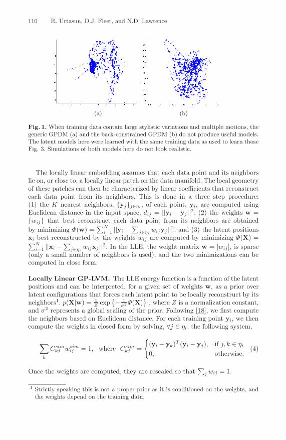
Fig. 1. When training data contain large stylistic variations and multiple motions, thegeneric GPDM (a) and the back-constrained GPDM (b) do not produce useful models.The latent models here were learned with the same training data as used to learn thoseFig. 3. Simulations of both models here do not look realistic.

The locally linear embedding assumes that each data point and its neighborslie on, or close to, a locally linear patch on the data manifold. The local geometryof these patches can then be characterized by linear coefficients that reconstructeach data point from its neighbors. This is done in a three step procedure:(1) the K nearest neighbors, {yj}j∈ηi , of each point, yi, are computed usingEuclidean distance in the input space, dij = ||yi − yj ||2; (2) the weights w ={wij} that best reconstruct each data point from its neighbors are obtainedby minimizing Φ(w) =

∑Ni=1 ||yi −

∑j∈ηi

wijyj ||2; and (3) the latent positionsxi best reconstructed by the weights wij are computed by minimizing Φ(X) =∑N

i=1 ||xi −∑

j∈ηiwijxj ||2. In the LLE, the weight matrix w = [wij ], is sparse

(only a small number of neighbors is used), and the two minimizations can becomputed in close form.

Locally Linear GP-LVM. The LLE energy function is a function of the latentpositions and can be interpreted, for a given set of weights w, as a prior overlatent configurations that forces each latent point to be locally reconstruct by itsneighbors1. p(X|w) = 1

Z exp{− 1

σ2 Φ(X)}

, where Z is a normalization constant,and σ2 represents a global scaling of the prior. Following [18], we first computethe neighbors based on Euclidean distance. For each training point yi, we thencompute the weights in closed form by solving, ∀j ∈ ηi, the following system,

∑

k

Csimkj wsim

ij = 1, where Csimkj =

{(yi − yk)T (yi − yj), if j, k ∈ ηi

0, otherwise.(4)

Once the weights are computed, they are rescaled so that∑

j wij = 1.

1 Strictly speaking this is not a proper prior as it is conditioned on the weights, andthe weights depend on the training data.

Modeling Human Locomotion 111

Learning the locally linear GP-LVM is then equivalent to minimizing thenegative log posterior of the model, that is up to an additive constant equal to 2

LS = log p(Y|X, β) p(β) p(X|w)

=D

2ln |KY | +

12tr

(K−1

Y YYT)

+∑

i

ln βi +1σ2

N∑

i=1

‖xi −N∑

j=1

wijxj‖2 .(5)

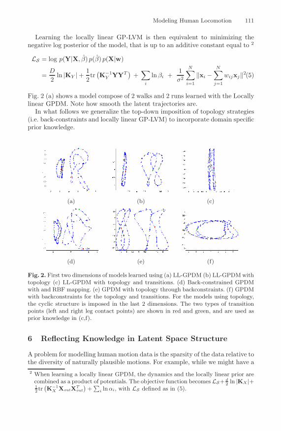
Fig. 2 (a) shows a model compose of 2 walks and 2 runs learned with the Locallylinear GPDM. Note how smooth the latent trajectories are.

In what follows we generalize the top-down imposition of topology strategies(i.e. back-constraints and locally linear GP-LVM) to incorporate domain specificprior knowledge.

(a) (b) (c)

(d) (e) (f)

Fig. 2. First two dimensions of models learned using (a) LL-GPDM (b) LL-GPDM withtopology (c) LL-GPDM with topology and transitions. (d) Back-constrained GPDMwith and RBF mapping. (e) GPDM with topology through backconstraints. (f) GPDMwith backconstraints for the topology and transitions. For the models using topology,the cyclic structure is imposed in the last 2 dimensions. The two types of transitionpoints (left and right leg contact points) are shown in red and green, and are used asprior knowledge in (c,f).

6 Reflecting Knowledge in Latent Space Structure

A problem for modelling human motion data is the sparsity of the data relative tothe diversity of naturally plausible motions. For example, while we might have a2 When learning a locally linear GPDM, the dynamics and the locally linear prior are

combined as a product of potentials. The objective function becomes LS+ d2 ln |KX |+

12 tr

(K−1

X XoutXTout

)+

∑i ln αi, with LS defined as in (5).

112 R. Urtasun, D.J. Fleet, and N.D. Lawrence

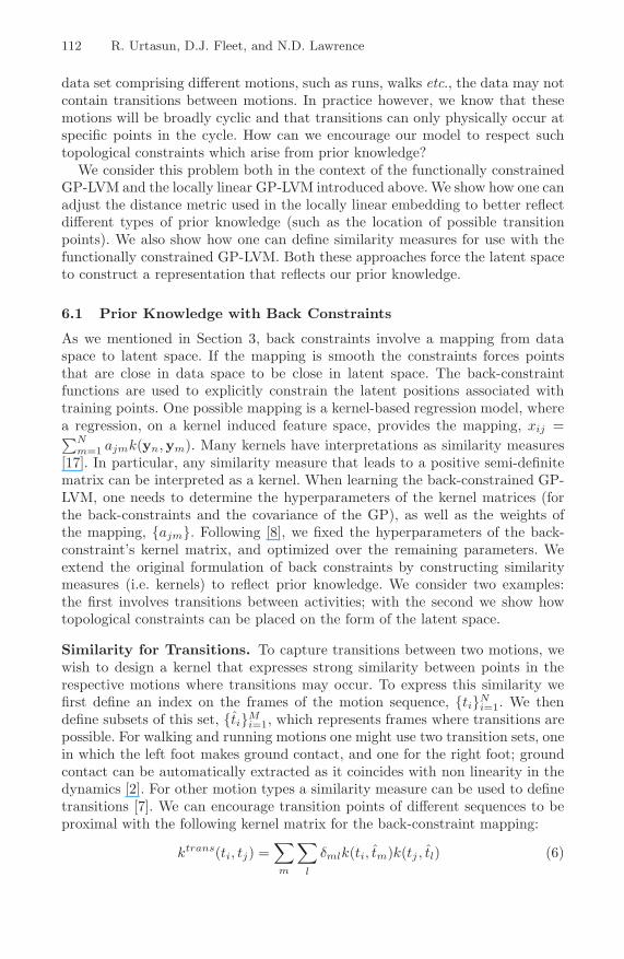
data set comprising different motions, such as runs, walks etc., the data may notcontain transitions between motions. In practice however, we know that thesemotions will be broadly cyclic and that transitions can only physically occur atspecific points in the cycle. How can we encourage our model to respect suchtopological constraints which arise from prior knowledge?

We consider this problem both in the context of the functionally constrainedGP-LVM and the locally linear GP-LVM introduced above. We show how one canadjust the distance metric used in the locally linear embedding to better reflectdifferent types of prior knowledge (such as the location of possible transitionpoints). We also show how one can define similarity measures for use with thefunctionally constrained GP-LVM. Both these approaches force the latent spaceto construct a representation that reflects our prior knowledge.

6.1 Prior Knowledge with Back Constraints

As we mentioned in Section 3, back constraints involve a mapping from dataspace to latent space. If the mapping is smooth the constraints forces pointsthat are close in data space to be close in latent space. The back-constraintfunctions are used to explicitly constrain the latent positions associated withtraining points. One possible mapping is a kernel-based regression model, wherea regression, on a kernel induced feature space, provides the mapping, xij =∑N

m=1 ajmk(yn,ym). Many kernels have interpretations as similarity measures[17]. In particular, any similarity measure that leads to a positive semi-definitematrix can be interpreted as a kernel. When learning the back-constrained GP-LVM, one needs to determine the hyperparameters of the kernel matrices (forthe back-constraints and the covariance of the GP), as well as the weights ofthe mapping, {ajm}. Following [8], we fixed the hyperparameters of the back-constraint’s kernel matrix, and optimized over the remaining parameters. Weextend the original formulation of back constraints by constructing similaritymeasures (i.e. kernels) to reflect prior knowledge. We consider two examples:the first involves transitions between activities; with the second we show howtopological constraints can be placed on the form of the latent space.

Similarity for Transitions. To capture transitions between two motions, wewish to design a kernel that expresses strong similarity between points in therespective motions where transitions may occur. To express this similarity wefirst define an index on the frames of the motion sequence, {ti}N

i=1. We thendefine subsets of this set, {ti}M

i=1, which represents frames where transitions arepossible. For walking and running motions one might use two transition sets, onein which the left foot makes ground contact, and one for the right foot; groundcontact can be automatically extracted as it coincides with non linearity in thedynamics [2]. For other motion types a similarity measure can be used to definetransitions [7]. We can encourage transition points of different sequences to beproximal with the following kernel matrix for the back-constraint mapping:

ktrans(ti, tj) =∑

m

∑

l

δmlk(ti, tm)k(tj , tl) (6)

Modeling Human Locomotion 113

where k(ti, tl) is an RBF centered at tl, and δml = 1 if tm and tl are in the sameset. The ‘strength’ of the encouragement is controlled by the support width ofthe RBF kernel.

Combining Similarities. One advantage of our framework is that kernel ma-trices can be combined in a principled manner to form new kernel matrices. Ker-nels can be multiplied (on an element by element basis) or added together. Mul-tiplication of kernel-based similarity measures has, loosely speaking, an ‘ANDgate effect’, i.e. both similarity measures must agree that an object is similar fortheir product to express similarity. Adding them produces more of an ‘OR gateeffect’, i.e. if either representation expresses similarity the resulting measure willalso express similarity.

Topologically Constrained Latent Spaces. We now consider kernels thatencourage the latent space to have a particular topology. Specifically we are in-terested in suitable topologies for walking and running data. Because the dataare approximately periodic, it seems appropriate to have a non-Cartesian topol-ogy. To this end one could extract the phase of the motion3, φ, and use itwith a suitable similarity measure to encourage the latent points to response anon-Cartesian topology within a Cartesian space. As an illustrative example weconsider a cylindrical topology within a three dimensional latent space by con-straining two of the latent dimensions with phase. In particular to represent thecyclic motion we construct a distance function on the unit circle, where a latentpoint corresponding to phase φ is represented with the point (cos(φ), sin(φ)). Aperiodic mapping can be constructed from a kernel matrix as follows,

xn,1 = gcos1 (yn, φn) =

N∑

m=1

acosm k(cos(φn), cos(φm)) + acos

0 δn,m,

xn,2 = gsin2 (yn, φn) =

N∑

m=1

asinm k(sin(φn), sin(φm)) + asin

0 δn,m,

where k is an RBF kernel function, and xn,i is the ith coordinate of the nth

latent point. These two mappings project onto two dimensions of the latentspace, forcing them to have a periodic structure (which comes about through thedependence of the kernel with respect to cosine and sine of the phase). Fig. 2 (e)shows a model learned using GPDM with the last two dimensions constrained inthis way (the third dimension is out of plane). The first dimension is constrainedby an RBF mapping on the input space. Each dimension’s kernel matrix canthen be augmented by adding the transition similarity given in (6), resulting inthe model depicted by Fig. 2 (f).

3 The phase can be easily extracted from the data by Fourier analysis or by detectingkey postures and interpolating the phases between them. Another idea, not furtherexplored here, would be to optimize the GP-LVM with respect to the phase.

114 R. Urtasun, D.J. Fleet, and N.D. Lawrence

6.2 Prior Knowledge Through Local Linearities

We now turn to consider how one might incorporate prior knowledge in thelocally linear GP-LVM framework. This is accomplished by replacing the localEuclidean distance measures presented in Section 5.1 with other similarity mea-sures. The standard Euclidean distance measure leads to the covariance matricegiven in (4). However, just as we developed similarity matrices above, we canalso modify this covariance function to reflect our prior knowledge in the latentspace.

Covariance for Transitions. To capture transitions in the latent model wedefine the elements for the covariance matrix as follows,

Ctransij = 1 −

[δij exp(−ζ(ti − tj)2)

](7)

with ζ a constant, and δij = 1 if ti and tj are in the same set {tk}Mk=1, and

otherwise δij = 0. This covariance encourages the points at which transitionsare physically possible to be close together in the latent space.

Combining Covariances. As above the covariance matrices can also be com-bined in a principled way. Covariances can be added or multiplied (on an elementby element basis) to loosely speaking produce and ‘OR’ or ‘AND’ gate effect.

Covariance for Topologies. To force a cylindrical topology on the latentspace, we can introduce covariances based on the phase, specifying differentcovariances for each latent dimensions. As before we construct a distance functionin the unit circle, that takes into account the phase.

Ccosj,k =

(cos(φi) − cos(φηj )

)(cos(φi) − cos(φηk

)) (8)

Csinj,k =

(sin(φi) − sin(φηj )

)(sin(φi) − sin(φηk

)) , (9)

The covariance for the remaining dimension is constructed as usual, based onEuclidean distance in the data space. In Fig. 2 (b) a GPDM is constrained inthis way, and in Fig. 2 (c) the covariance is augmented with transitions.

Note that the use of different distance measures for each dimension of thelatent space implies that the neighborhood and the weights in the locally linearprior will also be different for each dimension. One way of looking at it is thatthree different locally linear embeddings are developed for constructing the priordistribution. Each gives a prior distribution for a different dimension of the latentspace.

6.3 Model Combination

The two sections above have shown how to incorporate prior knowledge in theGP-LVM by means of 1) local linearities and 2) backconstraints. In general, thelatter converges faster but it is more intuitive to constraint the latent spacewith soft constraints. Both techniques are complementary and can be combinedstraightforwardly by including priors over some dimensions, and constraining theothers through back-constraint mappings. Fig. 3 shows a model learned with thelocally linear GPDM to impose smoothness and backconstraints for topology.

Modeling Human Locomotion 115

(a) (b) (c)

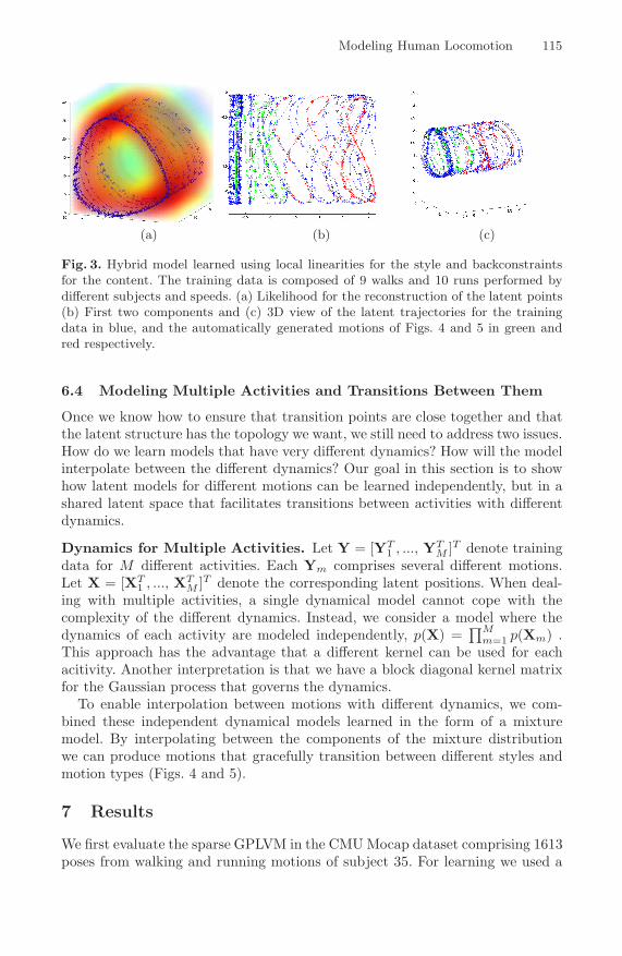
Fig. 3. Hybrid model learned using local linearities for the style and backconstraintsfor the content. The training data is composed of 9 walks and 10 runs performed bydifferent subjects and speeds. (a) Likelihood for the reconstruction of the latent points(b) First two components and (c) 3D view of the latent trajectories for the trainingdata in blue, and the automatically generated motions of Figs. 4 and 5 in green andred respectively.

6.4 Modeling Multiple Activities and Transitions Between Them

Once we know how to ensure that transition points are close together and thatthe latent structure has the topology we want, we still need to address two issues.How do we learn models that have very different dynamics? How will the modelinterpolate between the different dynamics? Our goal in this section is to showhow latent models for different motions can be learned independently, but in ashared latent space that facilitates transitions between activities with differentdynamics.

Dynamics for Multiple Activities. Let Y = [YT1 , ..., YT

M ]T denote trainingdata for M different activities. Each Ym comprises several different motions.Let X = [XT

1 , ..., XTM ]T denote the corresponding latent positions. When deal-

ing with multiple activities, a single dynamical model cannot cope with thecomplexity of the different dynamics. Instead, we consider a model where thedynamics of each activity are modeled independently, p(X) =

∏Mm=1 p(Xm) .

This approach has the advantage that a different kernel can be used for eachacitivity. Another interpretation is that we have a block diagonal kernel matrixfor the Gaussian process that governs the dynamics.

To enable interpolation between motions with different dynamics, we com-bined these independent dynamical models learned in the form of a mixturemodel. By interpolating between the components of the mixture distributionwe can produce motions that gracefully transition between different styles andmotion types (Figs. 4 and 5).

7 Results

We first evaluate the sparse GPLVM in the CMU Mocap dataset comprising 1613poses from walking and running motions of subject 35. For learning we used a

116 R. Urtasun, D.J. Fleet, and N.D. Lawrence

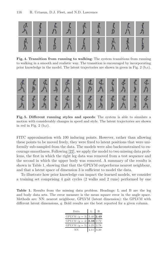
Fig. 4. Transition from running to walking: The system transitions from runningto walking in a smooth and realistic way. The transition is encouraged by incorporatingprior knowledge in the model. The latent trajectories are shown in green in Fig. 2 (b,c).

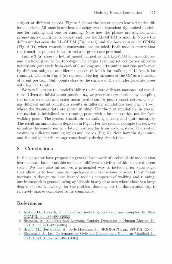
Fig. 5. Different running styles and speeds: The system is able to simulate amotion with considerably changes in speed and style. The latent trajectories are shownin red in Fig. 2 (b,c).

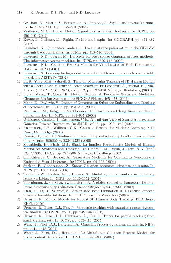
FITC approximation with 100 inducing points. However, rather than allowingthese points to be moved freely, they were fixed to latent positions that were uni-formily sub-sampled from the data. The models were also backconstrained to en-courage smoothness. Following [22], we apply the model to two missing data prob-lems, the first in which the right leg data was removed from a test sequence andthe second in which the upper body was removed. A summary of the results isshown in Table 1, showing that that the GPLVM outperforms nearest neighbour,and that a latent space of dimension 3 is sufficient to model the data.

To illustrate how prior knowledge can impact the learned models, we considera training set comprising 4 gait cycles (2 walks and 2 runs) performed by one

Table 1. Results from the missing data problem. Headings: L and B are the legand body data sets. The error measure is the mean square error in the angle space.Methods are: NN: nearest neighbour, GPLVM (latent dimension): the GPLVM withdifferent latent dimensions, q. Bold results are the best reported for a given column.

Data L B

GPLVM (q = 3) 3.40 2.49

GPLVM (q = 4) 3.38 2.72

GPLVM (q = 5) 4.25 2.78

NN 4.11 3.20

Modeling Human Locomotion 117

subject at different speeds. Figure 2 shows the latent spaces learned under dif-ferent priors. All models are learned using two independent dynamical models,one for walking and one for running. Note how the phases are aligned whenpromoting a cylindrical topology, and how the LL-GPDM is smooth. Notice thedifference between the LL-GPDM (Fig. 2 (c)) and the backconstrained GPDM(Fig. 2 (f)) when transition constraints are included. Both models ensure thatthe transition points (shown in red and green) are proximal.

Figure 3 (a) shows a hybrid model learned using LL-GPDM for smoothness,and back-constraints for topology. The larger training set comprises approxi-mately one gait cycle from each of 9 walking and 10 running motions performedby different subjects at different speeds (3 km/h for walking, 6–12 km/h forrunning). Colors in Fig. 3 (a) represent the log variance of the GP as a functionof latent position. Only points close to the surface of the cylinder generate poseswith high certainty.

We now illustrate the model’s ability to simulate different motions and transi-tions. Given an initial latent position x0, we generate new motions by samplingthe mixture model, and using mean prediction for pose reconstruction. Choos-ing different initial conditions results in different simulations (see Fig. 3 (b-c),where the training data are shown in blue). For the first simulation (in green),the motion is initialized to a running pose, with a latent position not far fromwalking poses. The system transitions to walking quickly and quite naturally.The resulting animation is depicted in Fig. 4. For the second example (in red), weinitialize the simulation to a latent position far from walking data. The systemevolves to different running styles and speeds (Fig. 5). Note how the dynamics,and the strike length, change considerably during simulation.

8 Conclusions

In this paper we have proposed a general framework of probabilistic models thatlearn smooth latent variable models of different activities within a shared latentspace. We have also introduced a principled way to include prior knowledge,that allow us to learn specific topologies and transitions between the differentmotions. Although we have learned models composed of walking and running,our framework is general, being applicable in any data sets where there is a largedegree of prior knowledge for the problem domain, but the data availability isrelatively sparse compared to its complexity.

References

1. Arikan, O., Forsyth, D.: Interactive motion generation from examples. In: SIG-GRAPH, pp. 483–490 (2002)

2. Bissacco, A.: Modeling and Learning Contact Dynamics in Human Motion. In:CVPR, pp. 421–428 (2005)

3. Brand, M., Hertzmann, A.: Style Machines. In: SIGGRAPH, pp. 183–192 (2000)4. Elgammal, A., Lee, C.: Separating Style and Content on a Nonlinear Manifold. In:

CVPR, vol. 1, pp. 478–485 (2004)

118 R. Urtasun, D.J. Fleet, and N.D. Lawrence

5. Grochow, K., Martin, S., Hertzmann, A., Popovic, Z.: Style-based inverse kinemat-ics. In: SIGGRAPH, pp. 522–531 (2004)

6. Vasilescu, M.A.: Human Motion Signatures: Analysis, Synthesis. In: ICPR, pp.456–460 (2002)

7. Kovar, L., Gleicher, M., Pighin, F.: Motion Graphs. In: SIGGRAPH, pp. 473–482(2002)

8. Lawrence, N., Quinonero-Candela, J.: Local distance preservation in the GP-LVMthrough back constraints. In: ICML, pp. 513–520 (2006)

9. Lawrence, N.D., Seeger, M., Herbrich, R.: Fast sparse Gaussian process methods:The informative vector machine. In: NIPS, pp. 609–616 (2003)

10. Lawrence, N.D.: Gaussian Process Models for Visualisation of High DimensionalData. In: NIPS (2004)

11. Lawrence, N.: Learning for larger datasets with the Gaussian process latent variablemodel. In: AISTATS (2007)

12. Li, R., Yang, M.H., Sclaroff, S., Tian, T.: Monocular Tracking of 3D Human Motionwith a Coordinated Mixture of Factor Analyzers. In: Leonardis, A., Bischof, H., Pinz,A. (eds.) ECCV 2006. LNCS, vol. 3952, pp. 137–150. Springer, Heidelberg (2006)

13. Li, Y., Wang, T., Shum, H.: Motion Texture: A Two-Level Statistical Model forCharacter Motion Synthesis. In: SIGGRAPH, pp. 465–472 (2002)

14. Moon, K., Pavlovic, V.: Impact of Dynamics on Subspace Embedding and Trackingof Sequences. In: CVPR, pp. 198–205 (2006)

15. Pavlovic, J.M., Rehg, J., MacCormick, J.: Learning switching linear models ofhuman motion. In: NIPS, pp. 981–987 (2000)

16. Quinonero-Candela, J., Rasmussen, C.E.: A Unifying View of Sparse ApproximateGaussian Process Regression. In: JMLR, vol. 6, pp. 1939–1959 (2006)

17. Rasmussen, C.E., Williams, C.K.: Gaussian Process for Machine Learning. MITPress, Cambridge (2006)

18. Roweis, S., Saul, L.: Nonlinear dimensionality reduction by locally linear embed-ding. Science 290(5500), 2323–2326 (2000)

19. Sidenbladh, H., Black, M.J., Sigal, L.: Implicit Probabilistic Models of HumanMotion for Synthesis and Tracking. In: Tistarelli, M., Bigun, J., Jain, A.K. (eds.)ECCV 2002. LNCS, pp. 784–800. Springer, Heidelberg (2002)

20. Sminchisescu, C., Jepson, A.: Generative Modeling for Continuous Non-LinearlyEmbedded Visual Inference. In: ICML, pp. 96–103 (2004)

21. Snelson, E., Ghahramani, Z.: Sparse Gaussian processes using pseudo-inputs. In:NIPS, pp. 1257–1264 (2006)

22. Taylor, G.W., Hinton, G.E., Roweis, S.: Modeling human motion using binarylatent variables. In: NIPS, pp. 1345–1352 (2007)

23. Tenenbaum, J., de Silva, V., Langford, J.: A global geometric framework for non-linear dimensionality reduction. Science 290(5500), 2319–2323 (2000)

24. Tian, T., Li, R., Sclaroff, S.: Articulated Pose Estimation in a Learned SmoothSpace of Feasible Solutions. In: CVPR Learning Workshop (2005)

25. Urtasun, R.: Motion Models for Robust 3D Human Body Tracking. PhD thesis,EPFL (2006)

26. Urtasun, R., Fleet, D.J., Fua, P.: 3d people tracking with gaussian process dynam-ical models. In: CVPR, vol. 1, pp. 238–245 (2006)

27. Urtasun, R., Fleet, D.J., Hertzman, A., Fua, P.: Priors for people tracking fromsmall training sets. In: ICCV, pp. 403–410 (2005)

28. Wang, J., Fleet, D.J., Hertzman, A.: Gaussian Process dynamical models. In: NIPS,pp. 1441–1448 (2005)

29. Wang, J., Fleet, D.J., Hertzman, A.: Multifactor Gaussian Process Models forStyle-Content Separation. In: ICML, pp. 975–982 (2007)