UNIVERSITÉ DE MONTRÉAL

MODÈLES D’OPTIMISATION STOCHASTIQUE POUR LE PROBLÈME DE GESTIONDE RÉSERVOIRS

CHARLES GAUVINDÉPARTEMENT DE MATHÉMATIQUES ET DE GÉNIE INDUSTRIEL

ÉCOLE POLYTECHNIQUE DE MONTRÉAL

THÈSE PRÉSENTÉE EN VUE DE L’OBTENTIONDU DIPLÔME DE PHILOSOPHIÆ DOCTOR

(MATHÉMATIQUES DE L’INGÉNIEUR)MAI 2017

c© Charles Gauvin, 2017.

UNIVERSITÉ DE MONTRÉAL

ÉCOLE POLYTECHNIQUE DE MONTRÉAL

Cette thèse intitulée :

MODÈLES D’OPTIMISATION STOCHASTIQUE POUR LE PROBLÈME DE GESTIONDE RÉSERVOIRS

présentée par : GAUVIN Charlesen vue de l’obtention du diplôme de : Philosophiæ Doctora été dûment acceptée par le jury d’examen constitué de :

M. AUDET Charles, Ph. D., présidentM. GENDREAU Michel, Ph. D., membre et directeur de rechercheM. DELAGE Erick, Ph. D., membre et codirecteur de rechercheM. BASTIN Fabian, Ph. D., membreM. GEORGHIOU Angelos, Ph. D., membre externe

iii

REMERCIEMENTS

Bien que la réalisation de cette thèse n’ait pas toujours été une expérience facile ni agréable,je suis reconnaissant de la richesse des expériences personnelles et professionnelles que j’aivécues au cours de ces quatre dernières années. J’ai eu l’opportunité d’en apprendre plus surun très large spectre de sujets en plus de développer une certaine expertise dans des domainespassionnants.

Avant toute chose, j’aimerais mettre l’accent sur la chance que j’ai eu au cours de monparcours. Sans chance, je n’aurais pu intégrer la maîtrise à Polytechnique, car je n’avais pasles compétences de base nécessaires. Je n’aurais pas non plus pu poursuivre au doctorat nirencontrer Erick, qui est devenu mon codirecteur.

Je tiens à remercier Michel de m’avoir supervisé au cours de ces quatre années. Bien que j’aiegrandement bénéficié de sa très vaste expérience, je retiens particulièrement son côté humainet ses encouragements à certains moments clés.

Je suis également reconnaissant à Erick de m’avoir encadré. J’apprécie maintenant sa granderigueur et minutie. Ses suggestions ont considérablement amélioré la qualité de mes travauxet m’ont très bien guidé. Je suis privilégié d’avoir pu le côtoyer, car il représente assurémentl’un des meilleurs chercheurs en recherche opérationnelle que j’ai eu la chance de rencontrer.C’est aussi grâce à lui que j’ai pu visiter le groupe du professeur Kuhn à Lausanne, ce qui aété un voyage extraordinaire.

I want to thank Daniel Kuhn as well as everyone in the RAO group at EPFL, namely Dirk,Grani, Napat, Peyman, Soroosh and Viet (ordered arbitrarily). My stay in Switzerland wasmemorable thanks to your kindness and the dynamic atmosphere of the lab.

Mes pensées se tournent ensuite vers tous les gens du GERAD que j’ai pu rencontrer au coursde ma maîtrise et de mon doctorat. Comme j’ai passé beaucoup de temps au laboratoire, jene pourrais nommer tous les gens que j’ai eu la chance de côtoyer sans oublier de noms. Leurprésence a cependant fortement contribué à enrichir et agrémenter mon expérience.

Merci aux gens d’Hydro-Québec et de l’IREQ de m’avoir fourni les données et la probléma-tique mais surtout de judicieux conseils. Je suis particulièrement reconnaissant à GrégoryÉmiel, Pierre-Marc Rondeau, Louis Delorme, Pierre-Luc Carpentier, Laura Fagherazzi ainsiqu’Alexia Marchand. Je suis également reconnaissant du support financier d’Hydro-Québecet du CRSNG.

Je tiens à souligner l’importance des discussions que j’ai eu avec Pascal Côté et Sara Séguin

iv

de Rio Tinto. Leur expertise et intérêt pour le problème de gestion hydroélectrique m’ontpermis de clarifier et de remettre en question plusieurs points.

Merci à Charles Audet, Fabian Bastin et Richard Gourdeau d’avoir lu ma thèse avec autantde minutie et d’intérêt en plus de m’avoir fait des commentaires d’une grande pertinence.

I would like to thank Angelos for accepting my invitation to be on my Ph.D. defense com-mittee and taking the time to give me such insightful comments. I am privileged to have sucha prolific researcher review my work.

J’ai également été touché par l’accueil que j’ai reçu au CIRRELT à Québec. Merci à YanCimon et Pierre Marchand de m’avoir trouvé un endroit pour travailler ainsi que de leurbonne humeur. Merci également à Jean-François Côté, Géraldine Heilporn, Leandro Coelhoet Bernard Lamond pour les nombreuses opportunités qu’ils m’ont présentées.

Je remercie également tous les gens qui m’ont encouragé à poursuivre des études supérieureset qui m’ont donné des opportunités d’effectuer de la recherche, notamment Paul Intrevado,Geneviève Bassellier et Liette Lapointe. Merci également à Guy Desaulniers pour son ex-cellent encadrement durant ma maîtrise.

I would also like to take the time to thank Jeroen Struben for the support and enthusiasm hedisplayed while I was still an undergraduate student at McGill. His supervision and teachinghad a profound impact on the way I think in general as well as my desire to pursue research.

Merci à Didier, Éric, Charles, Philippe, Cédric, Étienne, Carl-André et Marc (dans un ordrearbitraire) pour leur amitié au cours de ces nombreuses années.

Merci à toute ma famille pour leur support constant et leurs nombreuses attentions. Je suischoyé de toujours pouvoir compter sur eux.

Finalement, je remercie Caroline, l’amour de ma vie, pour ses nombreux encouragements aucours de ces dernières années. Elle est sans contredit la personne qui a le plus contribué àcette thèse et je lui en serai toujours reconnaissant.

v

RÉSUMÉ

La gestion d’un système hydroélectrique représente un problème d’une grande complexitépour des compagnies comme Hydro-Québec ou Rio Tinto. Il faut effectivement faire uncompromis entre plusieurs objectifs comme la sécurité des riverains, la production hydro-électrique, l’irrigation et les besoins de navigation et de villégiature. Les opérateurs doiventégalement prendre en compte la topologie du terrain, les délais d’écoulement, les interdé-pendances entre les réservoirs ainsi que plusieurs phénomènes non linéaires physiques. Mêmedans un cadre déterministe, ces nombreuses contraintes opérationnelles peuvent mener à desproblèmes irréalisables sous certaines conditions hydrologiques.

Par ailleurs, la considération de la production hydroélectrique complique considérablementla gestion du bassin versant. Une modélisation réaliste nécessite notamment de prendre encompte la hauteur de chute variable aux centrales, ce qui mène à un problème non convexe.

En outre, de nombreuses sources d’incertitude entourent la réalisation d’un plan de produc-tion. Les prix de l’électricité sur les marchés internationaux, la disponibilité des turbines,la charge/demande du réseau ainsi que les apports en eau sont tous incertains au momentd’établir les soutirages et les déversés pour un horizon temporel donné. Négliger cette incer-titude et supposer une connaissance parfaite du futur peut mener à des politiques de gestionbeaucoup trop ambitieuses. Ces dernières ont tendance à engendrer des conséquences désas-treuses comme le vidage ou le remplissage très rapide des réservoirs, ce qui conduit ensuiteà des inondations ou des sécheresses importantes.

Cette thèse considère le problème de gestion de réservoirs avec incertitude sur les apports. Elletente spécifiquement de développer des modèles et des algorithmes permettant d’améliorer lagestion mensuelle de la rivière Gatineau, notamment en période de crue. Dans cette situation,il est primordial de considérer l’incertitude autour des apports, car ces derniers ont uneinfluence marquée sur l’état hydrologique du système en plus d’être la cause d’évènementsdésastreux comme les inondations.

La gestion des inondations est particulièrement importante pour la Gatineau, car la rivièrecoule près de la ville de Maniwaki qui a déjà vécu des inondations dans le passé et continuede présenter des risques importants. Cette rivière représente également une excellente étudede cas, car elle possède plusieurs barrages et réservoirs. La grande dimension du système renddifficile l’application de certains algorithmes populaires comme la programmation dynamiquestochastique.

vi

Afin de minimiser le risque d’inondations, on propose initialement un modèle de programma-tion stochastique multi-étapes (multi-stage stochastic program) basé sur les règles de décisionaffine et les règles de décision affines liftées. On considère l’aversion au risque en évaluantla valeur à risque conditionnelle (conditional value-at-risk) aussi connue comme "CVaR".Ce travail considère une représentation polyhédrale de l’incertitude très simple basée sur lamoyenne et la variance d’échantillon.

Le deuxième article propose d’améliorer cette représentation de l’incertitude en considérantexplicitement la corrélation temporelle entre les apports. À cet effet, il introduit les modèles deséries chronologiques de type ARIMA et présente une manière de les incorporer efficacementdans un modèle multi-étapes avec règles de décision. On étend ensuite l’approche pour évaluerles processus GARCH, ce qui permet d’incorporer l’hétéroscédasticité.

Le troisième travail raffine la représentation de l’incertitude utilisée dans le deuxième travailen s’appuyant sur un modèle ARMA calibré sur le logarithme des apports. Cette représenta-tion non linéaire mène à un ensemble d’incertitude non convexe qu’on choisit d’approximer defaçon conservatrice par un polyhèdre. Ce modèle offre néanmoins plusieurs avantages commela possibilité de dériver une expression analytique pour l’espérance conditionnelle. Afin deconsidérer la hauteur de chute variable, on propose un algorithme de région de confiance trèssimple, mais efficace.

Ces travaux montrent qu’il est possible d’obtenir de bons résultats pour le problème degestion de réservoir en considérant les règles de décision linéaires en combinaison avec unereprésentation basée sur les processus ARIMA.

vii

ABSTRACT

The problem of designing an optimal release schedule for a hydroelectric system is extremelychallenging for companies like Rio Tinto and Hydro-Québec. It is essential to strike anadequate compromise between various conflicting objectives such a riparian security, hydro-electric production as well as navigation and irrigation needs. Operators must also considerthe topology of the terrain, water delays, dependence between reservoirs as well as non-linearphysical phenomena. Even in a deterministic framework, it may be impossible to find afeasible solution under given hydrological conditions.

Considering hydro-electricity generation further complicates the problem. Indeed, a realisticmodel must take into account variable water head, which leads to an intractable bilinearnon-convex problem.

In addition, there exists various sources of uncertainty surrounding the elaboration of theproduction plan. The price of electricity on foreign markets, availability of turbines, loadof the network and water inflows all remain uncertain at the time of fixing water releasesand spills over the given planning horizon. Neglecting this uncertainty and assuming perfectforesight will lead to overly ambitious policies. These decisions will in turn generate disastrousconsequences such as very rapid emptying or filling of reservoirs, which in turn generatedroughts or floods.

This thesis considers the reservoir management problem with uncertain inflows. It aims atdeveloping models and algorithms to improve the management of the Gatineau river, namelyduring the freshet. In this situation, it is essential to consider the randomness of inflows sincethese drive the dynamics of the systems and can lead to disastrous consequences like floods.

Flood management is particularly important for the Gatineau, since the river runs near thetown of Maniwaki, which has witnessed several floods in the past. This river also represents agood case study because it comprises various reservoirs and dams. This multi-dimensionalitymakes it difficult to apply popular algorithms such as stochastic dynamic programming.

In order to minimize the risk of floods, we initially propose a multi-stage stochastic pro-gram based on affine and lifted decision rules. We capture risk aversion by optimizing theconditional value-at-risk also known as "CVaR". This work considers a simple polyhedraluncertainty representation based on the sample mean and variance.

The second paper builds on this work by explicitly considering the serial correlation betweeninflows. In order to do so, it introduces ARIMA time series models and details their in-

viii

corporation into multi-stage stochastic programs with decision rules. The approach is thenextended to take into account heteroscedasticity with GARCH models

The third work further refines the uncertainty representation by calibrating an ARMA modelon the log of inflows. This leads to a non-convex uncertainty set, which is approximated witha simple polyhedron. This model offers various advantages such as increased forecastingskill and ability to derive an analytical expression for the conditional expectation. In orderto consider the variable water head, we propose a successive linear programming (SLP)algorithm which quickly yields good solutions.

These works illustrate the value of using affine decision rules in conjunction with ARIMAmodels to obtain good quality solutions to complex multi-stage stochastic problems.

ix

TABLE DES MATIÈRES

REMERCIEMENTS . . . . . . . . . . . . . . . . . . . . . . . . . . . . . . . . . . . . iii

RÉSUMÉ . . . . . . . . . . . . . . . . . . . . . . . . . . . . . . . . . . . . . . . . . . v

ABSTRACT . . . . . . . . . . . . . . . . . . . . . . . . . . . . . . . . . . . . . . . . vii

TABLE DES MATIÈRES . . . . . . . . . . . . . . . . . . . . . . . . . . . . . . . . . ix

LISTE DES TABLEAUX . . . . . . . . . . . . . . . . . . . . . . . . . . . . . . . . . xiv

LISTE DES FIGURES . . . . . . . . . . . . . . . . . . . . . . . . . . . . . . . . . . . xv

LISTE DES SIGLES ET ABRÉVIATIONS . . . . . . . . . . . . . . . . . . . . . . . xvii

CHAPITRE 1 INTRODUCTION . . . . . . . . . . . . . . . . . . . . . . . . . . . . 11.1 Production hydroélectrique . . . . . . . . . . . . . . . . . . . . . . . . . . . . 21.2 Gestion de la rivière Gatineau . . . . . . . . . . . . . . . . . . . . . . . . . . 5

1.2.1 La rivière . . . . . . . . . . . . . . . . . . . . . . . . . . . . . . . . . 51.2.2 Les apports . . . . . . . . . . . . . . . . . . . . . . . . . . . . . . . . 81.2.3 Gestion historique des réservoirs . . . . . . . . . . . . . . . . . . . . . 9

1.3 Objectifs de recherche . . . . . . . . . . . . . . . . . . . . . . . . . . . . . . 111.3.1 Modélisation . . . . . . . . . . . . . . . . . . . . . . . . . . . . . . . 121.3.2 Résolution . . . . . . . . . . . . . . . . . . . . . . . . . . . . . . . . . 121.3.3 Simulation et ajustement . . . . . . . . . . . . . . . . . . . . . . . . . 13

1.4 Plan du mémoire . . . . . . . . . . . . . . . . . . . . . . . . . . . . . . . . . 13

CHAPITRE 2 REVUE DE LITTÉRATURE . . . . . . . . . . . . . . . . . . . . . . 142.1 Modèles de séries chronologiques de type ARIMA . . . . . . . . . . . . . . . 14

2.1.1 Modèles univariés stationnaires . . . . . . . . . . . . . . . . . . . . . 142.1.2 Modèles non stationnaires . . . . . . . . . . . . . . . . . . . . . . . . 172.1.3 Modèles GARCH . . . . . . . . . . . . . . . . . . . . . . . . . . . . . 182.1.4 Modèles de séries chronologiques multivariées . . . . . . . . . . . . . 18

2.2 Programmation dynamique stochastique (Stochastic dynamic programming -SDP) . . . . . . . . . . . . . . . . . . . . . . . . . . . . . . . . . . . . . . . . 192.2.1 Cas général, dépendance arbitraire entre les apports . . . . . . . . . . 21

x

2.2.2 Cas où les apports sont indépendants . . . . . . . . . . . . . . . . . . 212.2.3 Cas (V)AR(p), corrélation d’ordre p ∈ N . . . . . . . . . . . . . . . . 212.2.4 Autres modélisations des variables hydrologiques . . . . . . . . . . . . 222.2.5 Améliorations permettant de réduire les malédictions de la dimensionalité 22

2.3 Programmation stochastique dynamique par échantillonnage (Sampling sto-chastic dynamic programming - SSDP) . . . . . . . . . . . . . . . . . . . . . 23

2.4 Programmation stochastique dynamique duale (Stochastic dual dynamic pro-gramming - SDDP) . . . . . . . . . . . . . . . . . . . . . . . . . . . . . . . . 242.4.1 Phase arrière - borne supérieure (pour un problème de maximisation) 242.4.2 Phase avant - borne inférieure . . . . . . . . . . . . . . . . . . . . . . 25

2.5 Programmation stochastique sur arbre . . . . . . . . . . . . . . . . . . . . . 262.6 Règles de décision linéaires/affines (Linear/affine decision rules) . . . . . . . 28

2.6.1 Mesures de risque . . . . . . . . . . . . . . . . . . . . . . . . . . . . . 33

CHAPITRE 3 ORGANISATION DE LA THÈSE . . . . . . . . . . . . . . . . . . . 37

CHAPITRE 4 ARTICLE 1: DECISION RULE APPROXIMATIONS FOR THE RISKAVERSE RESERVOIR MANGEMENT PROBLEM . . . . . . . . . . . . . . . . 394.1 Introduction . . . . . . . . . . . . . . . . . . . . . . . . . . . . . . . . . . . . 394.2 Description of the deterministic reservoir management problem (RMP) . . . 43

4.2.1 Basic model . . . . . . . . . . . . . . . . . . . . . . . . . . . . . . . . 434.2.2 Considering floods . . . . . . . . . . . . . . . . . . . . . . . . . . . . 454.2.3 Evaluating floods over the entire horizon for the whole hydro electrical

complex . . . . . . . . . . . . . . . . . . . . . . . . . . . . . . . . . . 464.3 Incorporating inflow uncertainty . . . . . . . . . . . . . . . . . . . . . . . . . 474.4 Risk analysis . . . . . . . . . . . . . . . . . . . . . . . . . . . . . . . . . . . 47

4.4.1 Conditional value-at-risk . . . . . . . . . . . . . . . . . . . . . . . . . 474.4.2 Dynamic risk measures and time consistency . . . . . . . . . . . . . . 49

4.5 Stochastic model and choice of decision rules . . . . . . . . . . . . . . . . . . 494.5.1 Affine decision rules . . . . . . . . . . . . . . . . . . . . . . . . . . . . 494.5.2 Objective function formulation for robust problem . . . . . . . . . . . 504.5.3 Affine decision rules on lifted probability space . . . . . . . . . . . . . 51

4.6 Case study . . . . . . . . . . . . . . . . . . . . . . . . . . . . . . . . . . . . . 534.6.1 The river system . . . . . . . . . . . . . . . . . . . . . . . . . . . . . 534.6.2 The inflows . . . . . . . . . . . . . . . . . . . . . . . . . . . . . . . . 554.6.3 Upper bounds on the risk of floods . . . . . . . . . . . . . . . . . . . 564.6.4 Evaluating the policies through simulation . . . . . . . . . . . . . . . 61

xi

4.6.5 Comparison with stochastic model based on a scenario tree . . . . . . 614.6.6 Simulation results . . . . . . . . . . . . . . . . . . . . . . . . . . . . . 624.6.7 Real scenarios results . . . . . . . . . . . . . . . . . . . . . . . . . . . 664.6.8 Brief comparison of budgeted and box uncertainty . . . . . . . . . . . 69

4.7 Conclusion . . . . . . . . . . . . . . . . . . . . . . . . . . . . . . . . . . . . . 734.8 Acknowledgments . . . . . . . . . . . . . . . . . . . . . . . . . . . . . . . . . 744.9 Appendix . . . . . . . . . . . . . . . . . . . . . . . . . . . . . . . . . . . . . 74

4.9.1 Representative robust constraint under standard affine decision rulesand box uncertainty . . . . . . . . . . . . . . . . . . . . . . . . . . . 74

4.9.2 Representative robust constraint under standard affine decision rulesand budgeted uncertainty . . . . . . . . . . . . . . . . . . . . . . . . 75

4.9.3 Equality constraints under standard affine decision rules . . . . . . . 764.9.4 Details on lifted decision rules with example . . . . . . . . . . . . . . 76

CHAPITRE 5 ARTICLE 2: A STOCHASTIC PROGRAM WITH TIME SERIES ANDAFFINE DECISION RULES FOR THE RESERVOIR MANAGEMENT PROBLEM 835.1 Introduction . . . . . . . . . . . . . . . . . . . . . . . . . . . . . . . . . . . . 83

5.1.1 Notation . . . . . . . . . . . . . . . . . . . . . . . . . . . . . . . . . . 875.2 The stochastic reservoir management problem . . . . . . . . . . . . . . . . . 87

5.2.1 Deterministic look-ahead model for flood minimization . . . . . . . . 875.2.2 Sources of uncertainty . . . . . . . . . . . . . . . . . . . . . . . . . . 905.2.3 General framework . . . . . . . . . . . . . . . . . . . . . . . . . . . . 905.2.4 Affine decision rules . . . . . . . . . . . . . . . . . . . . . . . . . . . . 915.2.5 Minimizing flood risk . . . . . . . . . . . . . . . . . . . . . . . . . . . 92

5.3 Exploiting time series models and linear decision rules . . . . . . . . . . . . . 935.3.1 General inflow representation . . . . . . . . . . . . . . . . . . . . . . 935.3.2 Considering general ARMA models . . . . . . . . . . . . . . . . . . . 945.3.3 Support of the joint distribution of the %t . . . . . . . . . . . . . . 975.3.4 Support of the (conditional) joint distribution of the ξt . . . . . . . 995.3.5 Considering heteroscedasticity . . . . . . . . . . . . . . . . . . . . . . 995.3.6 Additional modelling considerations . . . . . . . . . . . . . . . . . . . 1015.3.7 Optimizing the conditional expected flood penalties with affine decision

rules . . . . . . . . . . . . . . . . . . . . . . . . . . . . . . . . . . . . 1015.4 Monte Carlo simulation and rolling horizon framework . . . . . . . . . . . . 1045.5 Case study . . . . . . . . . . . . . . . . . . . . . . . . . . . . . . . . . . . . . 105

5.5.1 The river system . . . . . . . . . . . . . . . . . . . . . . . . . . . . . 105

xii

5.5.2 Historical daily inflows . . . . . . . . . . . . . . . . . . . . . . . . . . 1075.5.3 Forecasting daily inflows . . . . . . . . . . . . . . . . . . . . . . . . . 1085.5.4 Heteroscedastic inflows . . . . . . . . . . . . . . . . . . . . . . . . . . 1095.5.5 Comparing forecasts . . . . . . . . . . . . . . . . . . . . . . . . . . . 1105.5.6 Numerical experiments . . . . . . . . . . . . . . . . . . . . . . . . . . 1115.5.7 Simulations with ARMA(1,1) & GARCH(1,1) generator . . . . . . . 1125.5.8 Simulation with different time series model . . . . . . . . . . . . . . . 1135.5.9 Real Scenarios . . . . . . . . . . . . . . . . . . . . . . . . . . . . . . . 114

5.6 Conclusion . . . . . . . . . . . . . . . . . . . . . . . . . . . . . . . . . . . . . 1165.7 Acknowledgments . . . . . . . . . . . . . . . . . . . . . . . . . . . . . . . . . 1185.8 Appendix . . . . . . . . . . . . . . . . . . . . . . . . . . . . . . . . . . . . . 118

5.8.1 Joint probabilistic guarantees for the polyhedral support . . . . . . . 1185.8.2 Equivalent reformulation of the stochastic program according to % . . 1195.8.3 Deriving the robust/deterministic equivalent . . . . . . . . . . . . . . 1205.8.4 Details on GARCH(m, s) model . . . . . . . . . . . . . . . . . . . . . 1225.8.5 Forecast skill with synthetic ARMA(1,1) time series . . . . . . . . . . 124

CHAPITRE 6 ARTICLE 3: A SUCCESSIVE LINEAR PROGRAMMING ALGORITHMWITH NON-LINEAR TIME SERIES FOR THE RESERVOIR MANAGEMENTPROBLEM . . . . . . . . . . . . . . . . . . . . . . . . . . . . . . . . . . . . . . . 1266.1 Nomenclature . . . . . . . . . . . . . . . . . . . . . . . . . . . . . . . . . . . 127

6.1.1 Sets and parameters . . . . . . . . . . . . . . . . . . . . . . . . . . . 1276.1.2 Decision variables . . . . . . . . . . . . . . . . . . . . . . . . . . . . . 1286.1.3 Random variables . . . . . . . . . . . . . . . . . . . . . . . . . . . . . 128

6.2 Introduction . . . . . . . . . . . . . . . . . . . . . . . . . . . . . . . . . . . . 1286.3 Deterministic formulation . . . . . . . . . . . . . . . . . . . . . . . . . . . . 130

6.3.1 Daily river operations . . . . . . . . . . . . . . . . . . . . . . . . . . . 1306.3.2 Biobjective problem . . . . . . . . . . . . . . . . . . . . . . . . . . . . 134

6.4 Incorporating uncertainty . . . . . . . . . . . . . . . . . . . . . . . . . . . . 1356.5 Stochastic multi-stage formulation . . . . . . . . . . . . . . . . . . . . . . . . 136

6.5.1 Affine decision rules . . . . . . . . . . . . . . . . . . . . . . . . . . . . 1366.5.2 Objective function and composite risk . . . . . . . . . . . . . . . . . . 1376.5.3 Using successive linear programming to approximate the true problem 1376.5.4 Rolling horizon simulation . . . . . . . . . . . . . . . . . . . . . . . . 138

6.6 The Gatineau river system . . . . . . . . . . . . . . . . . . . . . . . . . . . . 1386.7 Numerical experiments . . . . . . . . . . . . . . . . . . . . . . . . . . . . . . 140

xiii

6.7.1 Daily inflows . . . . . . . . . . . . . . . . . . . . . . . . . . . . . . . 1406.7.2 Model performance under hard synthetic scenario compared with al-

ternative inflow representations . . . . . . . . . . . . . . . . . . . . . 1406.7.3 Model performance under realistic historical conditions compared with

historical decisions . . . . . . . . . . . . . . . . . . . . . . . . . . . . 1416.7.4 Exploring the solution space . . . . . . . . . . . . . . . . . . . . . . . 143

6.8 Conclusion . . . . . . . . . . . . . . . . . . . . . . . . . . . . . . . . . . . . . 145Acknowledgment . . . . . . . . . . . . . . . . . . . . . . . . . . . . . . . . . . . . 1456.9 Appendix . . . . . . . . . . . . . . . . . . . . . . . . . . . . . . . . . . . . . 145

6.9.1 Details on Ξt . . . . . . . . . . . . . . . . . . . . . . . . . . . . . . . 1456.9.2 Analytical expression for the composite risk . . . . . . . . . . . . . . 1496.9.3 First order Taylor approximation of the composite risk . . . . . . . . 151

CHAPITRE 7 DISCUSSION GÉNÉRALE . . . . . . . . . . . . . . . . . . . . . . . 1527.1 Synthèse des travaux . . . . . . . . . . . . . . . . . . . . . . . . . . . . . . . 1527.2 Limitations de la solution proposée . . . . . . . . . . . . . . . . . . . . . . . 1537.3 Améliorations futures . . . . . . . . . . . . . . . . . . . . . . . . . . . . . . . 154

7.3.1 Représentation des apports pour le premier article . . . . . . . . . . 1547.3.2 Représentation des apports pour le deux derniers articles . . . . . . . 1557.3.3 Conséquence additionnelle d’une représentation plus fine des apports 1597.3.4 Utilisation d’un modèle hydrologique . . . . . . . . . . . . . . . . . . 1617.3.5 Modélisation des courbes d’évacuation . . . . . . . . . . . . . . . . . 1617.3.6 Résolution en horizon roulant sur un plus long horizon et réplication

de la politique de gestion . . . . . . . . . . . . . . . . . . . . . . . . . 162

CHAPITRE 8 CONCLUSION . . . . . . . . . . . . . . . . . . . . . . . . . . . . . . 164

RÉFÉRENCES . . . . . . . . . . . . . . . . . . . . . . . . . . . . . . . . . . . . . . . 165

xiv

LISTE DES TABLEAUX

Tableau 1.1 Classification typique des problèmes d’optimisation hydroélectrique . 1Tableau 1.2 Proportion de l’eau soutirée du réservoir immédiatement en amont au

jour t se rendant au réservoir au jour t+ l . . . . . . . . . . . . . . . 6Tableau 4.1 Decision variables . . . . . . . . . . . . . . . . . . . . . . . . . . . . . 44Tableau 4.2 Comparison of optimal values and solution times . . . . . . . . . . . 58Tableau 4.3 Size of robust equivalents (standard affine vs. lifted) . . . . . . . . . . 59Tableau 4.4 Number of Simplex/Barrier iterations and solution times . . . . . . . 60Tableau 4.5 Size of robust equivalents (box vs. budget) . . . . . . . . . . . . . . . 71Tableau 6.1 Impact of different uncertainty representations . . . . . . . . . . . . . 140Tableau 6.2 Energy generation increase (%) with model water head . . . . . . . . 143

xv

LISTE DES FIGURES

Figure 1.1 Vue en coupe d’une centrale hydroélectrique . . . . . . . . . . . . . . 3Figure 1.2 Puissance de référence pour une hauteur de chute et débits déversés

constants . . . . . . . . . . . . . . . . . . . . . . . . . . . . . . . . . 4Figure 1.3 Bassin versant de la rivière Gatineau . . . . . . . . . . . . . . . . . . 7Figure 1.4 Apports historiques journaliers aux différents points névralgiques de la

rivière . . . . . . . . . . . . . . . . . . . . . . . . . . . . . . . . . . . 9Figure 1.5 Volumes historiques journaliers aux différents réservoirs . . . . . . . . 11Figure 2.1 Filtres linéaires . . . . . . . . . . . . . . . . . . . . . . . . . . . . . . 17Figure 2.2 Arbre de scénario symétrique . . . . . . . . . . . . . . . . . . . . . . 26Figure 2.3 Arbre de scénario asymétrique . . . . . . . . . . . . . . . . . . . . . . 27Figure 4.1 Simplified representation of the Gatineau river system . . . . . . . . . 53Figure 4.2 Evacuation curves . . . . . . . . . . . . . . . . . . . . . . . . . . . . . 54Figure 4.3 Violations with perfect foresight . . . . . . . . . . . . . . . . . . . . . 55Figure 4.4 Sample observations (Y = 6 years) for inflows . . . . . . . . . . . . . 56Figure 4.5 Impact of number of simplex iterations on total computing times . . 60Figure 4.6 Sample multistage tree generated by SCENRED2 from scenario fan . 62Figure 4.7 Empirical CVaRα of violations accross policies with log-normally simu-

lated random variables and α ∈ 0, 0.5, 1 for a fixed reservoir . . . . 64Figure 4.8 Empirical CVaRα of violations across reservoirs with log-normally si-

mulated random variables for a fixed policy . . . . . . . . . . . . . . 65Figure 4.9 Actual values . . . . . . . . . . . . . . . . . . . . . . . . . . . . . . . 68Figure 4.10 Impact of different uncertainty sets on simulation results . . . . . . . 70Figure 4.11 Impact of different uncertainty sets on real historical inflows . . . . . 72Figure 4.12 Image of polyhedron under a bijective linear mapping and bounding box 77Figure 4.13 Lt([lt, ut]) and conv(Lt([lt, ut])), t = 1, 2. . . . . . . . . . . . . . . . . 78Figure 5.1 Sequential Dynamic Decision Process . . . . . . . . . . . . . . . . . . 91Figure 5.2 Simplified representation of the Gatineau river system . . . . . . . . . 106Figure 5.3 Sample inflows for 1999-2004 and 2008-2013 (12 years) with "in-sample"

mean . . . . . . . . . . . . . . . . . . . . . . . . . . . . . . . . . . . . 107Figure 5.4 Comparing simple forecasts for 1999 & 2002 . . . . . . . . . . . . . . 109Figure 5.5 Residuals from ARMA(1,1) model . . . . . . . . . . . . . . . . . . . 110Figure 5.6 Influence of reduced forecast skill . . . . . . . . . . . . . . . . . . . . 112Figure 5.7 Influence of increased unconditional variance . . . . . . . . . . . . . 113

xvi

Figure 5.8 Influence of different time series structure . . . . . . . . . . . . . . . 114Figure 5.9 Simulation results for 1999-2004 & 2008-2013 (12 years) . . . . . . . 115Figure 6.1 Flow chart for the rolling horizon simulation algorithm . . . . . . . . 138Figure 6.2 Reference production functions . . . . . . . . . . . . . . . . . . . . . 139Figure 6.3 Model results on hard historical scenario . . . . . . . . . . . . . . . . 142Figure 6.4 Exploring the solution space . . . . . . . . . . . . . . . . . . . . . . . 144Figure 6.5 Non convex uncertainty set . . . . . . . . . . . . . . . . . . . . . . . 149Figure 7.1 Relation entre les apports totaux ∑j ξjt et les apports aux différents

réservoirs ξjt . . . . . . . . . . . . . . . . . . . . . . . . . . . . . . . . 154Figure 7.2 Relation entre les apports à Baskatong, Maniwaki et Rapides-Farmer 156

xvii

LISTE DES SIGLES ET ABRÉVIATIONS

(S)AR(I)MA (Seasonal) Autoregressive (Integrated) Moving AverageCVaR Conditional Value At RiskGARCH Generalized Autoregressive Conditional HeteroscedasticMSE Mean Square ErrorSDDP Stochastic Dual Dynamic ProgrammingSDP Stochastic Dynamic ProgrammingSLP Successive Linear ProgrammingSOCP Second Order Cone ProgrammingSSDP Sampling Stochastic Dynamic ProgrammingVaR Value At Risk

1

CHAPITRE 1 INTRODUCTION

Hydro-Québec représente l’un des plus grands producteurs d’électricité au monde. Tirantla quasi-totalité de son énergie de l’hydro-électricité, la société d’état est responsable dela gestion de plus de 80 centrales hydroélectriques et quelques unités thermales avec unecapacité installée de plus de 36 000 MW (Hydro-Québec, 2015). Elle dispose également d’unevingtaine de réservoirs de forte contenance et plus de 600 barrages répartis en quatre zonesgéographiques distinctes.

L’optimisation d’un tel parc de production représente un problème d’une complexité énorme.Il faut effectivement considérer un problème de très grande dimension avec des objectifs mul-tiples parfois contradictoires, des contraintes non convexes pouvant être difficiles à modéliserainsi que de nombreuses sources d’incertitude s’étalant sur un horizon temporel parfois trèslong.

Afin de trouver des solutions opérationnelles à un tel problème, on procède à une décompo-sition du problème en plusieurs sous-étapes, de façon similaire à ce qui est fait dans d’autresdomaines comme le transport aérien (Saddoune, 2010) et la foresterie (Rönnqvist, 2003).Dans le cas des problèmes d’optimisation hydroélectriques, on considère spécifiquement lamodélisation court (opérationnel), moyen (tactique) et long terme (stratégique) (voir le ta-bleau 1.1)

Tableau 1.1 Classification typique des problèmes de gestion hydroélectrique.

TypeHorizontemporeltypique

Pas detemps

Type dedécisions

Représentationdu parc

Importancede l’aléa

Courtterme 1 semaine - 1 mois horaire

opérationnelex : -vente et achatsur les marchés spot

et jour d’avant-production journalière

détaillée faible

Moyenterme 1-2 ans hebdomadaire

tactiqueex : -contrats à moyen terme

-évaluation desstocks saisonniers

moyenne moyenne

Longterme 5-10 ans mensuel

stratégiqueex : -investissements

-localisation de centralesagrégée élevée

Ces problèmes sont liés entre eux et les résultats des modèles plus agrégés sont utilisés afinde guider la résolution de modèles plus fins. Par exemple, la résolution de modèles moyenterme peut permettre d’obtenir des hyperplans afin de valoriser les stocks finaux d’eau dans

2

les réservoirs. Ces hyperplans peuvent ensuite être utilisés par des modèles court terme dansle but d’éviter de vider les réservoirs à la fin de l’horizon relativement court.

Cette thèse se penche spécifiquement sur un problème d’horizon court terme, à savoir lagestion mensuelle de la rivière Gatineau en présence d’incertitude sur les apports. Le modèlea notamment été développé dans l’optique de faciliter la gestion de la rivière en période decrue. Les sections qui suivent donnent plus de détails sur la gestion de la rivière ainsi que surla production hydroélectrique en général.

1.1 Production hydroélectrique 1

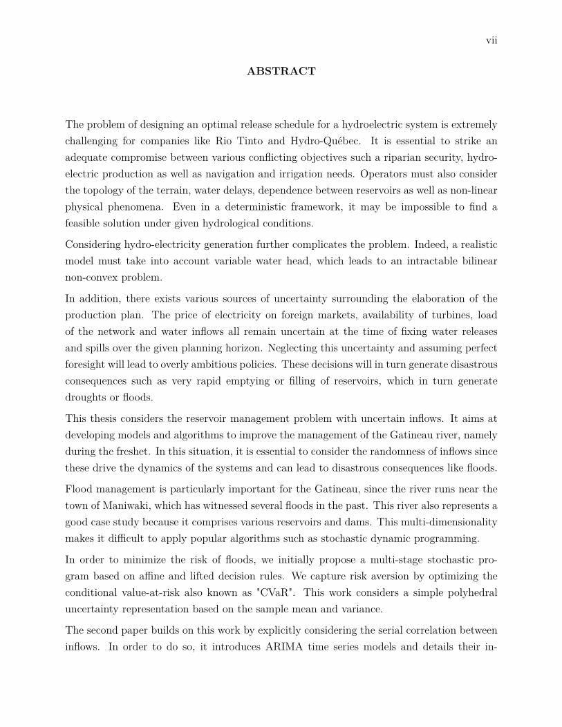
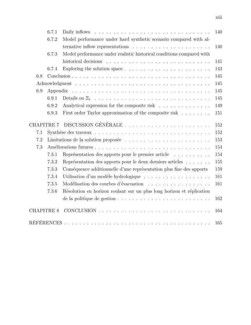
La production hydroélectrique exploite le cycle naturel d’évapotranspiration, condensation,précipitation et ruissellement/infiltration afin de convertir l’énergie potentielle de l’eau enénergie mécanique puis en énergie électrique (en plus de pertes d’énergie thermique). Cestransformations sont décrites à l’aide de la figure 1.1. 2

Le processus consiste initialement à stocker de l’énergie potentielle sous forme d’eau dansdes réservoirs (A). 3 En ouvrant les vannes (intake) (E), les opérateurs peuvent contrôler laquantité d’eau soutirée (released) qui sera ensuite amenée vers la conduite forcée (penstock),ce qui engendrera certaines pertes thermiques. Cette eau fera ensuite tourner les pales dela turbine (C), ce qui permettra de produire de l’électricité grâce au générateur (D) dans lacentrale (powerhouse/power plant) (B). L’électricité est finalement transportée par les ligneshaute tension (G), alors que l’eau s’écoule vers la rivière en aval (H).

1. Cette section est inspirée des travaux de Séguin (2016); Côté (2010).2. Pour assurer la cohésion et faciliter la lecture des chapitres 4 5 et 6, certains termes techniques anglais

correspondants sont indiqués en italique.3. Selon la capacité du réservoir, on dira que la centrale est une centrale à réservoir (conventional/dam

plant) ou une centrale au fil de l’eau (run-of-the-river plant).

3

Figure 1.1 Vue en coupe d’une centrale hydroélectrique. Adaptée avec permission de "Hy-droelectric dam" par Tomia, 2008. Image sous license GFDL et CC-BY-2.5.

La puissance générée (en MW) à un instant donné par une centrale est une fonction de lahauteur de chute (water head), c’est-à-dire de la différence (enm) entre le niveau d’eau ou biefamont et le niveau d’eau ou bief aval. La puissance dépend également des caractéristiquesdes turbines individuelles et de l’eau soutirée et déversée (en m3/s). Dans cette thèse, onconsidère une formulation plus agrégée que celle de Séguin (2016) et les groupes de turbinessont traités comme un seul bloc homogène. Par ailleurs, on suppose que toutes les turbinessont disponibles et fonctionnent à leur capacité normale. Cette hypothèse n’est pas toujoursvérifiée, car la pression de l’eau sur les pales ainsi que certains phénomènes de cavitationpeuvent engendrer des bris qui nécessitent des arrêts de maintenance. On ignore égalementles zones interdites, car ces dernières causent des difficultés numériques considérables et notresolution ne les considère jamais. La formule utilisée pour représenter P totaleit , la puissanceproduite (en MW) à tout instant durant le jour t à la centrale i prend la forme 4 :

P totalit (Rit,Lit,Hit) = Pit(Rit,Lit)Hit. (1.1)

où Pit(R,L) représente la puissance de référence, qui est fonction des débits soutirés Rit etdéversés Lit pour une hauteur de chute fixée. L’expression Hit indique quant à elle la hauteur

4. Cette représentation est notamment utilisée par Gjelsvik et al. (2010).

4

de chute relative, donnée par :

Hiτ = Nj−τ −Nj+τHrefi

(1.2)

où Hrefi représente la hauteur de chute de référence et Nj−t et Nj+τ représentent le niveau

d’eau amont (forebay) et aval (tailrace) (en m) à la centrale. Le niveau d’eau amont Nj−t estune fonction concave croissante du volume du réservoir Sjt. Pour la plupart des réservoirs, leniveau aval est considéré comme constant. Cependant, lorsque deux centrales sont très prèsl’une de l’autre, le niveau aval à une centrale est une fonction du volume à la centrale aval.

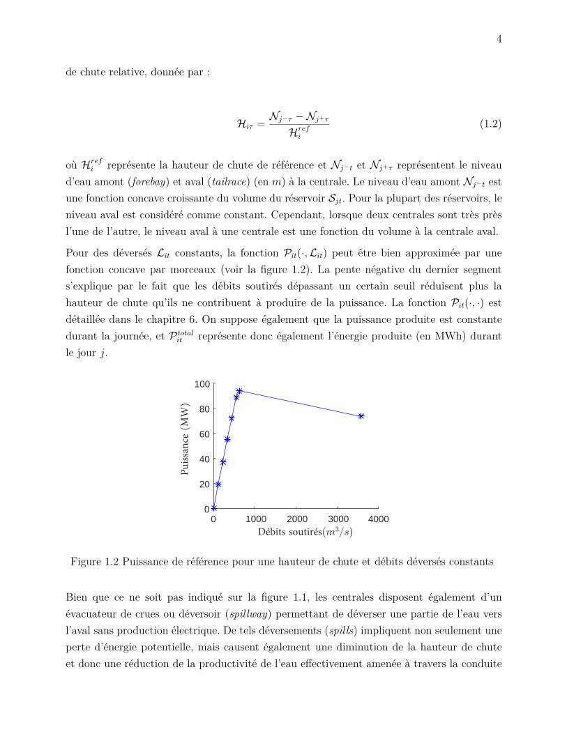
Pour des déversés Lit constants, la fonction Pit(·,Lit) peut être bien approximée par unefonction concave par morceaux (voir la figure 1.2). La pente négative du dernier segments’explique par le fait que les débits soutirés dépassant un certain seuil réduisent plus lahauteur de chute qu’ils ne contribuent à produire de la puissance. La fonction Pit(·, ·) estdétaillée dans le chapitre 6. On suppose également que la puissance produite est constantedurant la journée, et P totalit représente donc également l’énergie produite (en MWh) durantle jour j.

0 1000 2000 3000 4000 50000

50

100

150

200

250

Pow

er(M

Wh)

Plant - Paugan

0 40001000 2000 3000 Total flow (m3=s)

0

50

100

150

Pow

er(M

Wh)

Plant - Chelsea

0 40001000 2000 3000 Débits soutirés(m3=s)

0

20

40

60

80

100

Puiss

ance

(M

W)

Total flow (m3=s)

Reference production

Figure 1.2 Puissance de référence pour une hauteur de chute et débits déversés constants

Bien que ce ne soit pas indiqué sur la figure 1.1, les centrales disposent également d’unévacuateur de crues ou déversoir (spillway) permettant de déverser une partie de l’eau versl’aval sans production électrique. De tels déversements (spills) impliquent non seulement uneperte d’énergie potentielle, mais causent également une diminution de la hauteur de chuteet donc une réduction de la productivité de l’eau effectivement amenée à travers la conduite

5

pour produire de l’électricité.

1.2 Gestion de la rivière Gatineau

1.2.1 La rivière

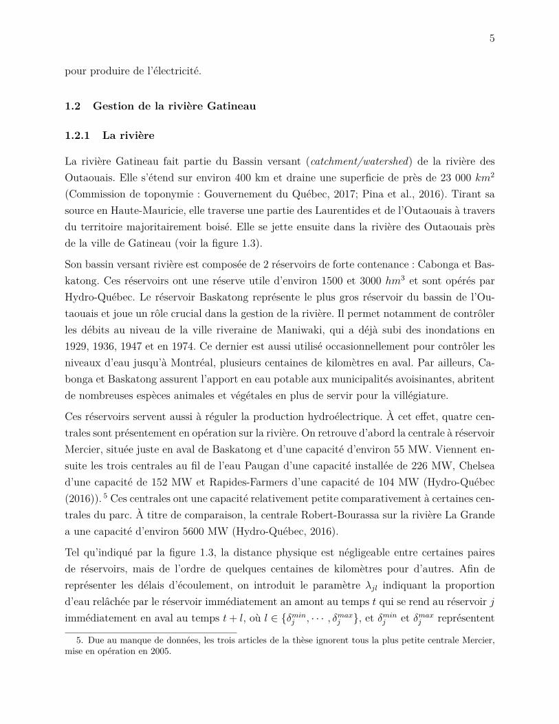
La rivière Gatineau fait partie du Bassin versant (catchment/watershed) de la rivière desOutaouais. Elle s’étend sur environ 400 km et draine une superficie de près de 23 000 km2

(Commission de toponymie : Gouvernement du Québec, 2017; Pina et al., 2016). Tirant sasource en Haute-Mauricie, elle traverse une partie des Laurentides et de l’Outaouais à traversdu territoire majoritairement boisé. Elle se jette ensuite dans la rivière des Outaouais prèsde la ville de Gatineau (voir la figure 1.3).

Son bassin versant rivière est composée de 2 réservoirs de forte contenance : Cabonga et Bas-katong. Ces réservoirs ont une réserve utile d’environ 1500 et 3000 hm3 et sont opérés parHydro-Québec. Le réservoir Baskatong représente le plus gros réservoir du bassin de l’Ou-taouais et joue un rôle crucial dans la gestion de la rivière. Il permet notamment de contrôlerles débits au niveau de la ville riveraine de Maniwaki, qui a déjà subi des inondations en1929, 1936, 1947 et en 1974. Ce dernier est aussi utilisé occasionnellement pour contrôler lesniveaux d’eau jusqu’à Montréal, plusieurs centaines de kilomètres en aval. Par ailleurs, Ca-bonga et Baskatong assurent l’apport en eau potable aux municipalités avoisinantes, abritentde nombreuses espèces animales et végétales en plus de servir pour la villégiature.

Ces réservoirs servent aussi à réguler la production hydroélectrique. À cet effet, quatre cen-trales sont présentement en opération sur la rivière. On retrouve d’abord la centrale à réservoirMercier, située juste en aval de Baskatong et d’une capacité d’environ 55 MW. Viennent en-suite les trois centrales au fil de l’eau Paugan d’une capacité installée de 226 MW, Chelsead’une capacité de 152 MW et Rapides-Farmers d’une capacité de 104 MW (Hydro-Québec(2016)). 5 Ces centrales ont une capacité relativement petite comparativement à certaines cen-trales du parc. À titre de comparaison, la centrale Robert-Bourassa sur la rivière La Grandea une capacité d’environ 5600 MW (Hydro-Québec, 2016).

Tel qu’indiqué par la figure 1.3, la distance physique est négligeable entre certaines pairesde réservoirs, mais de l’ordre de quelques centaines de kilomètres pour d’autres. Afin dereprésenter les délais d’écoulement, on introduit le paramètre λjl indiquant la proportiond’eau relâchée par le réservoir immédiatement an amont au temps t qui se rend au réservoir jimmédiatement en aval au temps t+ l, où l ∈ δminj , · · · , δmaxj , et δminj et δmaxj représentent

5. Due au manque de données, les trois articles de la thèse ignorent tous la plus petite centrale Mercier,mise en opération en 2005.

6

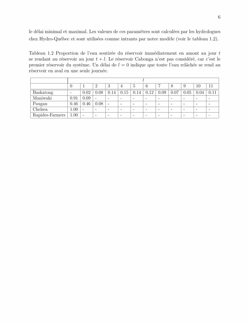
le délai minimal et maximal. Les valeurs de ces paramètres sont calculées par les hydrologueschez Hydro-Québec et sont utilisées comme intrants par notre modèle (voir le tableau 1.2).

Tableau 1.2 Proportion de l’eau soutirée du réservoir immédiatement en amont au jour tse rendant au réservoir au jour t + l. Le réservoir Cabonga n’est pas considéré, car c’est lepremier réservoir du système. Un délai de l = 0 indique que toute l’eau relâchée se rend auréservoir en aval en une seule journée.

l0 1 2 3 4 5 6 7 8 9 10 11

Baskatong - 0.02 0.08 0.14 0.15 0.14 0.12 0.09 0.07 0.05 0.04 0.11Maniwaki 0.91 0.09 - - - - - - - - - -Paugan 0.46 0.46 0.08 - - - - - - - - -Chelsea 1.00 - - - - - - - - - - -Rapides-Farmers 1.00 - - - - - - - - - - -

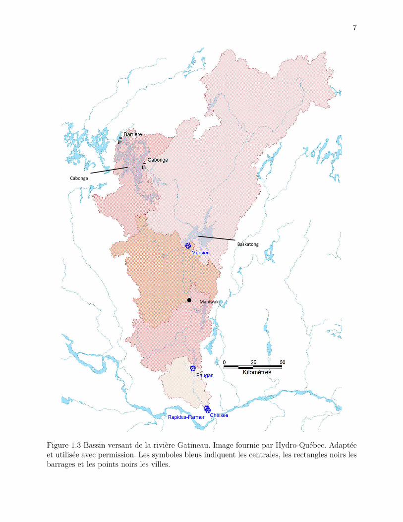
7

!

Baskatong

Cabonga

Maniwaki

Figure 1.3 Bassin versant de la rivière Gatineau. Image fournie par Hydro-Québec. Adaptéeet utilisée avec permission. Les symboles bleus indiquent les centrales, les rectangles noirs lesbarrages et les points noirs les villes.

8

1.2.2 Les apports

Dans un contexte de minimisation des inondations, les facteurs les plus importants à considé-rer sont les stocks initiaux d’eau dans les réservoirs ainsi que les apports en eau, qui demeurentincertains au moment de développer un plan d’opération. Comme l’indique la figure 1.4, cesderniers sont sujets à des variations saisonnières et inter-annuelles très importantes.

Durant l’hiver et le printemps, le régime hydraulique est principalement influencé par laprésence puis la fonte de neige. La crue printanière engendre notamment des apports trèsimportants dans un court laps de temps. Cette période est névralgique, car l’hydraulicitémoyenne et la variabilité y sont maximisées.

Pendant l’été, les apports sont faibles. Comme ce moment coïncide avec une période denavigation et d’achalandage accru sur la rivière, il est important de s’assurer que les niveauxd’eau minimaux soient respectés.

Suit ensuite une seconde crue en automne due à des précipitations plus importantes quedurant le reste de l’année. Pour certains réservoirs et certaines années, la crue automnale estencore plus critique que celle du printemps. La section 6 présente d’ailleurs une étude de casconsidérant la crue automnale de 2003.

9

0 500 1000 1500 2000

Jours (depuis 01/01/99)

0

200

400m

3/s

Cabonga

0 500 1000 1500 2000

Jours (depuis 01/01/99)

0

1000

2000

m3/s

Baskatong

0 500 1000 1500 2000

Jours (depuis 01/01/99)

0

100

200

300

m3/s

Maniwaki

0 500 1000 1500 2000

Jours (depuis 01/01/99)

0

100

200

m3/s

Paugan

0 500 1000 1500 2000

Jours (depuis 01/01/99)

0

100

200

m3/s

Chelsea

0 500 1000 1500 2000

Jours (depuis 01/01/99)

0

0.2

0.4

0.6

m3/s

Rapides-Farmers

Apports journaliers historiques Moyenne annuelle historique

Figure 1.4 Apports historiques journaliers aux différents points névralgiques de la rivière (enm3/s) de 1999-2004. Les barres grises verticales délimitent les 6 années.

1.2.3 Gestion historique des réservoirs

Hydro-Québec est tenu de gérer ses installations de façon intégrée en s’assurant de la sécuritédes opérations et en se concertant avec plusieurs groupes d’intérêts. Le risque d’inondationà Maniwaki est particulièrement important pour les opérateurs de la rivière, notamment enpériode de crue (freshet). Pour ces raisons, la rivière Gatineau est gérée de façon indépendantedu reste du parc de production.

Les apports ont une influence capitale sur la gestion des différents réservoirs. En effet, le

10

volume moyen d’apport en eau durant la crue printanière à Cabonga et Baskatong est de 590et 3630 hm3 et a même atteint 710 et 4700 hm3 en 1997. Ayant des capacités utiles d’environ1500 et 3000 hm3, ceci implique que ces réservoirs, particulièrement Baskatong, peuvent seremplir complètement en une seule crue. Les opérateurs utilisent donc un cycle de vidangeet de remplissage annuel pour Baskatong (voir la figure 1.5). Le 1er avril, aux alentours ducommencement de la crue printanière, on vise un niveau d’eau suffisamment faible permettantde remplir le réservoir tout en évitant les débits trop élevés en aval à Maniwaki.

Comme Cabonga reçoit moins d’eau par rapport à sa capacité et qu’il est possible d’évacuerune partie de son stock hors du bassin versant de la Gatineau vers le lac Barrière, le réservoiroffre plus de flexibilité et peut être utilisé afin de stocker ou de soutirer de l’eau selon laquantité d’apports.

Les stocks aux centrales au fil de l’eau sont quant à eux beaucoup plus variables d’unejournée et d’une année à l’autre. En effet, ces réservoirs ont une très petite contenance et ilspeuvent être vidés ou remplis complètement en quelques jours seulement. Ces niveaux d’eauvolatiles permettent aux opérateurs de tirer des avantages opérationnels dus à des variationsde hauteur de chute.

On note notamment que le réservoir Paugan est historiquement maintenu à son niveau maxi-mal, ce qui maximise la hauteur de chute. Les niveaux d’eau à Chelsea sont également main-tenus à des niveaux assez élevés, bien qu’il semble y exister des cycles interannuels causésnotamment par les apports ainsi que le désir des opérateurs de conserver une certaine margede manœuvre. Finalement, on observe que les niveaux d’eau à Rapides-Farmers ne dépassentjamais un seuil critique. Ceci est dû à la présence d’une crête déversante à la centrale. Cetouvrage d’évacuation ne permet pas aux opérateurs de contrôler directement les débits dé-versés. En effet, lorsque les stocks d’eau dépassent un certain niveau, une certaine proportionde l’eau est naturellement évacuée en aval. Comme ce déversement ne conduit pas à de laproduction hydroélectrique, les opérateurs choisissent de le minimiser.

11

0 20000

500

1000

1500

2000

hm3

Cabonga

0 20000

1000

2000

3000

4000

hm3

Baskatong

0 20000

50

100

hm3

500 1000 1500

Jours (depuis 01/01/99)Paugan

0 2000500 1000 1500

Jours (depuis 01/01/99)

0

2

4

6

hm3

500 1000 1500

Jours (depuis 01/01/99)

Chelsea

0 2000500 1000 1500

Jours (depuis 01/01/99)

0

1

2

3

hm3

500 1000 1500

Jours (depuis 01/01/99)Rapides-Farmers

Volume historique

Figure 1.5 Volumes historiques journaliers aux différents réservoirs de 1999-2004 (en hm3)

1.3 Objectifs de recherche

L’objectif de cette thèse est de concevoir des modèles mathématiques et des algorithmesdans le but de développer un outil d’aide à la décision facilitant la gestion de la rivière pourles opérateurs et permettant de réaliser certaines études exploratoires. À terme, cet outilpourrait même permettre d’améliorer ces opérations, notamment en aidant à concevoir desplans de production générant plus d’électricité tout en maintenant, ou même en réduisant,le risque d’inondations.

12

1.3.1 Modélisation

La première étape consiste à bien modéliser le problème. Il faut spécifiquement identifier unefonction objectif adéquate, la représentation de l’incertitude, les contraintes, ainsi que lesdécisions à prendre. Il est impératif de proposer une modélisation fidèle à la réalité permettantde s’assurer du respect de toutes les contraintes opérationnelles et satisfaisant les intérêts desdifférents groupes d’intérêt.

En présence d’aléa, la prise de décision prend la forme d’une politique de gestion, c’est-à-dire un ensemble de fonctions de l’incertitude. On optimise donc sur un espace fonctionnel,plutôt que sur un espace de variables comme c’est le cas en programmation mathématiquedéterministe.

Il faut ensuite déterminer la bonne fonctionnelle permettant d’évaluer l’objectif pour diffé-rents scénarios d’apports. Cette thèse utilise l’espérance mathématique, mais explore éga-lement quelques mesures de risque afin d’évaluer l’impact de l’aversion au risque sur lessolutions finales.

Tel que mentionné précédemment, la modélisation des apports est d’une importance crucialepour ce problème. Il faut donc savoir bien utiliser les techniques de modélisation statistique.Cette thèse exploite notamment les processus stochastiques à temps discrets de type ARIMA(autoregressive integrated moving average) pour bien représenter la corrélation temporelle. Lesarbres de décision, populaires en programmation stochastique multi-étapes, sont égalementexplorés dans le chapitre 4.

1.3.2 Résolution

La deuxième étape consiste à concevoir des algorithmes permettant de résoudre efficacementle problème. Il s’agit d’écrire du code informatique permettant de traduire le modèle théoriqueen format numérique pour enfin utiliser des solveurs commerciaux extrêmement efficacescomme CPLEX et Mosek afin de le résoudre.

L’outil devra être utilisable de façon opérationnelle. Ceci implique entres autres qu’il devrafournir des solutions de bonne qualité à l’intérieur de temps de calcul raisonnables, idéalementquelques secondes. Il devra permettre d’évaluer différents scénarios efficacement et de fournirdes réponses rapides afin de guider le choix des opérateurs.

13

1.3.3 Simulation et ajustement

Finalement, la dernière étape consiste à ajuster le modèle après avoir observé les résultatspréliminaires et les avoir confrontés aux scénarios réels. Il s’agit ici de concevoir un banc detest de simulation pour bien tester notre modèle. Encore une fois, plusieurs notions de statis-tiques et de processus hydrologiques deviennent utiles pour concevoir des scénarios d’apportsynthétiques réalistes et intéressants. L’étude de cas du chapitre 4 illustre notamment com-ment ces simulations permettent de mieux comprendre les hypothèses et les limitations denotre modèle. L’utilisation de scénarios historiques se révèle également essentielle pour aug-menter la crédibilité de nos travaux. Le chapitre 6 explique notamment que notre modèlepourrait améliorer les décisions historiques.

1.4 Plan du mémoire

Le chapitre 2 présente une revue de littérature des principales méthodes d’optimisation sto-chastique utilisées pour la gestion de réservoirs. Cette section survole également deux sujetsimportants pour la thèse : les mesures de risque et les séries chronologiques de type ARIMA.Le chapitre 3 dresse un portrait d’ensemble des 3 articles de la thèse, présentés aux chapitres4, 5 et 6. Finalement, le chapitre 8 tire des conclusions sur le travail réalisé et propose despistes de solutions futures.

14

CHAPITRE 2 REVUE DE LITTÉRATURE

2.1 Modèles de séries chronologiques de type ARIMA

Une partie importante de cette thèse se base sur la représentation des apports à l’aide desséries chronologiques à temps discret de type ARIMA. Ces processus linéaires paramétriquesoffrent plusieurs avantages. Ils possèdent une représentation linéaire compacte et facile àcomprendre, ont des propriétés bien étudiées, bénéficient de logiciels permettant de réaliserleur calibrage et ont été utilisés avec succès pour modéliser les apports. Cette section s’appuiefortement sur les trois références Box et al. (2008); Brockwell and Davis (1987) et Tsay (2005)

2.1.1 Modèles univariés stationnaires

Par souci de simplicité, on commence par traiter le cas univarié, c’est-à-dire qu’on considèred’abord un processus stochastique ζt∞t=−∞ où chaque ζt est une variable aléatoire réelle.

Avant de procéder à la description de ces processus, il est important de détailler certainsconcepts. On dit qu’un processus stochastique ζt∞t=−∞ est stationnaire 1 s’il respecte lespropriétés suivantes :

E [ζt] = µ, ∀t ∈ Z, (2.1)γ(h) = E [ζtζt+h] , ∀t, h ∈ Z, (2.2)E[ζ2t

]<∞, ∀t ∈ Z. (2.3)

L’équation (2.1) implique que le processus a une moyenne constante. Dans ce cas, on peuttoujours remplacer ζt par ζ ′t = ζt − µ et on peut donc supposer que µ = 0. L’équation (2.2)indique que la covariance dépend uniquement du déplacement h ∈ Z dans le temps et doncen particulier on obtient la variance γ(0) = σ2, qui est constante par rapport au temps, enévaluant γ(·) en 0. Finalement, (2.3) indique que le second moment est borné, ce qui impliqueque la variance est également bornée.

On s’intéresse notamment au processus stationnaire de bruit blanc %t qui possède les pro-priétés suivantes :

1. Il s’agit en fait d’hypothèse de stationnarité au sens large aussi connue sous le nom de stationnaritéfaible ou de second ordre.

15

γ(h) =

σ2 si h = 0

0 sinon ,∀h ∈ Z (2.4)

E [%t] = 0, ∀t ∈ Z. (2.5)

Bien qu’on ait uniquement besoin de ces conditions sur les deux premiers moments pourdévelopper les modèles de séries chronologiques, les chapitres 5 et 6 imposent des contraintesadditionnelles sur le support des %t. Le chapitre 5 supposent que les %t sont non corrélés etsuivent un processus GARCH (generalized autoregressive conditional heteroscedastic model),décrit dans les sections qui suivent. Le chapitre 6 fait des hypothèses plus fortes. Il supposenotamment que les %t suivent une distribution particulière et sont indépendants.

Étant donné le processus de bruit blanc %t décrit précédemment, on dit que le proces-sus stochastique ζt suit un processus ARMA(p, q) s’il est stationnaire et s’il respecte leséquations de différence suivantes pour tout t ∈ Z :

φ(B)ζt = θ(B)%t, (2.6)

où φ(B) = ∑pi=0 φiB

i et θ(B) = ∑qi=0 θiB

i représentent des polynômes. L’opérateur B permetd’effectuer un décalage dans le temps : Biζt = ζt−i. Les paramètres à calibrer sont les φi ∈ Roù i = 1, · · · , p et θj ∈ R où j = 1, · · · , q, pour des p, q ∈ N fixés. On impose toujoursφ0 = θ0 = 1.

La stationnarité de ζt est assurée si φ(z) 6= 0,∀z ∈ C : |z| ≤ 1. Dans ce cas, il existeψ(B) = ∑∞

i=0 ψiBi tel que ∑∞i=0 |ψi| <∞ et ψ(B) = φ−1(B)θ(B) de telle sorte que pour tout

t :

ψ(B)%t = φ−1(B)θ(B)%t = φ−1(B)φ(B)ζt = ζt2 (2.7)

La représentation (2.7) est d’une grande importance, car elle indique que les ζt peuvent êtreexprimés comme une combinaison linéaire infinie des résidus ou chocs passés : %s : s ≤ t. La

2. Pour résoudre cette équation, on considère φ(B)ψ(B) = θ(B) ⇔ (1 + ψ1B + ψ2B2 + · · · )(1 + φ1B +

φ2B2 + · · ·+φpB

p) = (1 + θ1B+ · · · θqBq) et on s’assure récursivement que la somme des coefficients des Bisoit égale à 0 pour tout i ∈ N. Par exemple : φ1 + ψ1 = θ1, φ2 + φ1ψ1 + ψ2 = θ2, etc.

16

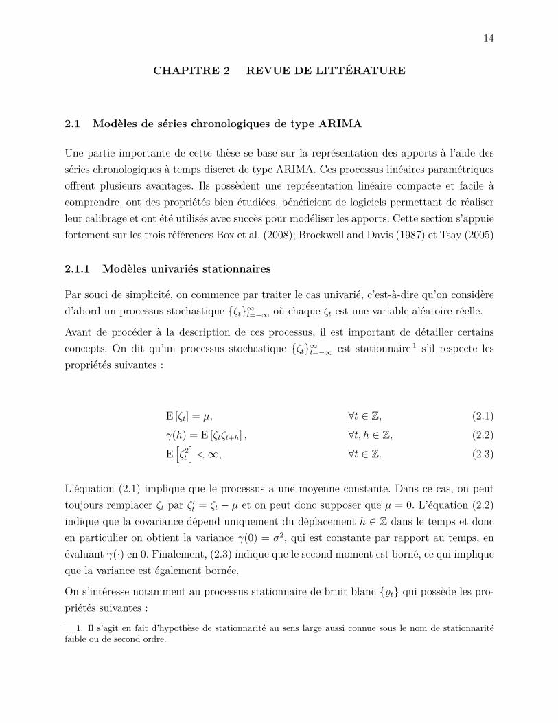
condition que la somme des coefficients ψi converge absolument assure que la limite existe etest unique dans un certain sens (Brockwell and Davis, 1987). Dans la littérature, on dit queψ(B) est un filtre linéaire ou une fonction de transfert. Tel que l’indique la figure 2.1, ψ(B)prend le bruit blanc %ss≤r non-corrélé en intrant et produit des ζt ayant une "corrélationplus structurée" comme extrant.

Cette représentation permet également de dériver une expression décomposable pratique poureffectuer des prévisions. En effet pour tout t ∈ Z et l ∈ N :

ζt+l =∞∑i=l

ψi%t+l−i︸ ︷︷ ︸ζt(l)

+l−1∑i=0

ψi%t+l−i︸ ︷︷ ︸ρt(l)

(2.8)

Le premier terme ζt(l) représente la prévision (forecast) effectuée au temps t pour un tempsfutur (lead time) de l périodes. Le deuxième terme ρt(l) représente donc l’erreur de prévision :ρt(l) = ζt+l − ζt(l). La prévision est donc déterministe sachant %sts=−∞, car elle dépenduniquement des résidus passés, qu’on suppose parfaitement observables. L’erreur de prévisionpeut quant à elle être exprimée comme un combinaison linéaire des résidus futurs : %st+ls=t+1.

Cette stationnarité dépend du polynôme φ(B). La condition correspondante : θ(z) 6= 0, ∀z ∈C : |z| ≤ 1 se nomme inversibilité. Dans ce cas, il existe π(B) = ∑∞

i=0 πiBi tel que ∑∞i=0 |πi| <

∞ et π(B) = θ−1(B)φ(B). La propriété suivante tient donc pour tout t :

%t = π(B)ζt. (2.9)

La propriété d’inversibilité assure entre autres que pour tout l ∈ N et f : Rt+l → R, lesespérances conditionnelles E

[f(ζ1, · · · , ζt+l)|ζ[t]

]et E

[f(ζ1, · · · , ζt+l)|%[t]

]sont identiques, car

l’information fournie par les %sts=−∞ est identique à celle fournie par ζsts=−∞.

Comme c’est presque toujours le cas dans la littérature, cette thèse considère uniquementdes processus stationnaires et inversibles. Ces deux conditions sont respectées si θ(z)φ(z) 6=0,∀z ∈ C : |z| ≤ 1. Il faut donc que les racines des polynômes θ(z) et φ(z) se trouvent àl’extérieur du cercle unitaire. Par exemple, on sait que le processus ARMA(1,1) utilisé auchapitre 5 respecte cette conditions, car on a : φ(z) = 1−0.96z et θ(z) = 1−0.13z. Les racinessont donc 0.96−1 > 1 et 0.13−1 > 1. Le processus AR(4) utilisé au chapitre 6 a également 4racines (complexes) à l’extérieur du cercle unitaire.

17

Sous les hypothèse de stationnarité et d’inversibilité, on a : ψ(B) = φ−1(B)θ(B) et π(B) =θ−1(B)φ(B). On a donc ψ(B)π(B) = 1 ou encore ψ−1(B) = π(B) et π−1(B) = θ(B). Tel quementionné dans Brockwell and Davis (1987), sous certaines autres hypothèses standards surles zéros des polynômes φ(z) et θ(z), on peut même garantir qu’il existe une seule solutionsatisfaisant (2.6).

A(B)

:(B)

1t%t

t t

Figure 2.1 Filtres linéaires

2.1.2 Modèles non stationnaires

On peut exprimer le polynôme φ(z) = 1 − φ1z − · · · − φpzp comme φ(z) = (1 − G1z)(1 −G2z) · · · (1−Gpz) où G−1

i sont les racines du polynôme φ(z).

Si φ(z) a k ∈ N racines unitaires et le reste de ses racines à l’extérieur du cercle unitaire, alors ilexiste K ⊂ 1, · · · , p; |K| = k tel que Gi = 1,∀i ∈ K ce qui implique φ(B) = φ′(B)(1−B)k

où φ′(z) 6= 0,∀z ∈ C : |z| ≤ 1. On peut donc appliquer l’analyse précédente sur la sériestationnaire : z′t = (1 − B)kzt. Par exemple si on a une tendance d’accroissement linéaire,alors il serait judicieux d’utiliser k = 1 et d’évaluer les différences (1 − B)zt = zt − zt−1 quisera stationnaire, même si les zt ne le sont pas Box et al. (2008). L’utilisation de l’opérateur(1−B)k conduit à un modèle (non-stationnaire) "intégré" d’ordre k, dénoté ARIMA(·, k, ·).

Un autre cas commun est celui où le polynôme φ(z) peut être exprimé comme φ(z) = φ′(z)(1−zs) pour un s ∈ N donné où φ′(z) 6= 0,∀z ∈ C : |z| ≤ 1. Dans ce cas, φ(z) a s racines surle cercle unitaire de la forme : e2πi k

s où√i = −1 et k = 0, 1, · · · , s − 1. La solution à

(1− Bs)zt = %t où %t représente du bruit blanc sera donc, en moyenne, une combinaison decosinus et sinus d’une périodicité de s périodes. L’utilisation de l’opérateur (1− zs) conduitici à l’ajout de la saisonnalité, d’où le "S" dans "SARIMA".

18

2.1.3 Modèles GARCH

Dans le cas le plus simple, les résidus %t sont supposés indépendants et on a E[ζ2t+l|%[t]

]=

E[ζ2t+l

]= σ2, peu importe l ∈ N. Si on relaxe cette hypothèse et qu’on suppose plutôt que les

résidus sont non corrélés et que les variances conditionnelles respectent la relation suivante :

σ2t−1(1) = α0 +

m∑i=1

αi%2t−i +

s∑j=1

βjσ2t−1−j(1) , (2.10)

où σ2t (l) = E

[%2t+l|%[t]

]pour tout l ∈ N, alors on dit que les résidus suivent un modèle

GARCH(m, s) (Bollerslev, 1986). Le terme hétéroscédasticité conditionnelle indique simple-ment que la variance conditionnelle n’est plus constante comme dans le cas où les %t sontindépendants. Ceci permet de modéliser plusieurs phénomènes tirés du monde réel, notam-ment en finance, où des périodes de volatilité accrues tendent à être suivies de périodesde variation élevée (Garcia et al., 2005; Tsay, 2005). Bien que les modèles GARCH n’aientpas été utilisés abondamment en gestion de réservoirs, Pianosi and Soncini-Sessa (2009) ontconsidéré cette forme d’incertitude dans un modèle réduit résolu "en ligne" pour gérer le lacVerbano sur la frontière italo-suisse.

Afin de s’assurer de la non-négativité de la variance conditionnelle, on impose des restrictionssur les coefficients : α0, αi, βj ≥ 0,∀i, j. En prenant l’espérance des deux côtés de (2.10) eten se rappelant que l’espérance est constante selon les hypothèses de stationnarité (2.4), ondérive également d’autres relations sur les coefficients.

Le chapitre 5 indique qu’en appliquant une transformation affine aux apports, le test sta-tistique Ljung-Box (Ljung and Box, 1978) permet de rejeter l’hypothèse que les %2

t sontindépendants, suggérant donc l’utilité d’un modèle GARCH. Par contre, l’utilisation du lo-garithme au chapitre 6 permet de contrôler ce phénomène et ne nécessite donc pas l’utilisationdu modèle GARCH.

2.1.4 Modèles de séries chronologiques multivariées

Cette thèse considère uniquement des processus stochastiques univariés en faisant des hypo-thèse simplificatrices sur la corrélation spatiale des apports à chaque pas de temps. Le cha-pitre 8 discute néanmoins de quelques améliorations possibles afin de considérer des modèlesplus réalistes. Ces représentations s’appuient sur des processus ARMA multidimensionnels(vectoriels) aussi appelés VARMA. Si ζt et %t représentent des vecteurs aléatoires de dimen-sion |J | pour tout t et Φi ∈ R|J |×|J |, i = 1, · · · , p, alors on pourrait notamment exploiter la

19

représentation :

ζt =p∑i=1

Φiζt−i + %t (2.11)

On note cependant que l’identification, le calibrage ainsi que la vérification des conditionsde stationnarité sont relativement plus complexes pour les modèles multivariés (Tsay, 2005).Ces derniers introduisent également certains phénomènes comme la colinéarité en plus denécessiter la sauvegarde de matrices de dimension |J | × |J | plutôt que des scalaires et sontsusceptibles d’augmenter considérablement la complexité du modèle. Bien que ces modèlessoient un peu plus rares dans la littérature, ils ont été considérés par certains chercheurscomme Gjelsvik et al. (2010) qui discute notamment de l’utilisation d’un modèle VAR(1).

2.2 Programmation dynamique stochastique (Stochastic dynamic programming- SDP)

La programmation dynamique stochastique représente l’une des méthodes les plus utiliséesen optimisation de petits systèmes sur un horizon moyen terme. Cette méthode bénéficie deplusieurs décennies de recherche et a été implantée avec succès pour déterminer les soutiragesmensuels et évaluer les stocks d’eau pour certains réservoirs opérés par Hydro-Québec.

Afin de décrire cette approche, on considère le problème de gestion de réservoirs en présenced’incertitude sur les apports. On le formule comme le problème de contrôle optimal suivantadapté de Turgeon (2005) et Séguin (2016) :

maxπt(·)

E[T∑t=1

Bt(xt, ut, ξt)]

: xt+1 = ft(xt, ut, ξt); xt ∈ Xt; ut ∈ Ut(xt, ξt); πt(xt) = ut

,

(2.12)

où on définit les concepts suivants :

— Les états : xt ∈ Xt ⊂ Rs comprennent habituellement les volumes de chaque réservoirau début du temps t ainsi qu’un sous-ensemble de l’historique des apports pour tenircompte de la corrélation temporelle. Le vecteur x0 est connu au temps 0.

— Les actions/décisions : ut ∈ Ut(xt, ξt) ⊂ Ra représentent habituellement les débitssoutirés (turbinés) et déversés. Le domaine Ut(xt, ξt) assure le respect des contraintes

20

opérationnelles.— L’incertitude : ξt ∈ Ξt ⊂ Rr représentent habituellement les apports aux différents

réservoirs.— Les fonctions de récompense : Bt : Xt × Ut × Ξt → R sont typiquement les fonc-

tions de production auxquelles on soustrait une pénalité pour des inondations et/oules déversés. Bt(·) peut être une fonction arbitraire, possiblement discontinue et nonconvexe.

— Les fonctions de transition : ft : Xt × Ut × Ξt → Rs représentent habituellement leséquations de conservation de masse (conservation de l’eau).

On cherche la politique optimale, c’est-à-dire les fonctions πt : Rs → Ra pour chaque t ∈T = 1, · · · , T qui maximisent (2.12). À cet effet, on exprime notre problème de manièrerécursive en exploitant le principe d’optimalité de Bellman. Ceci nécessite de définir Jt(xt)comme la fonction de valeur au temps t ∈ 1, · · · , T évaluée en xt, c’est-à-dire le coût espérédes opérations de t à T étant donné l’état actuel xt. Plus précisément :

JT (xT ) = Jval. eau(xT ) (2.13)

Jt(xt) = Eξt[

maxut∈Ut(xt,ξt)

Bt(xt, ut, ξt) + Jt+1(ft(xt, ut, ξt)) |ξt−1, · · · , ξ1

], t = 1, · · · , T − 1,

(2.14)

où Jval. eau(·) est la fonction valorisant le stock final d’eau. Cette fonction peut notammentêtre obtenue en résolvant un problème de gestion de réservoirs moyen terme. Les chapitres 4,5 et 6 considèrent le cas où Jval. eau(·) est affine, mais en général cette fonction est continueet non convexe.

Comme Jval. eau(·) et Bt(·) peuvent être des fonctions non convexes, le problème d’optimi-sation (2.14) est difficile en général et il faut procéder à une approximation. On supposesouvent dans la littérature qu’on discrétise les états, les actions et les réalisations de l’incerti-tude selon la même granularité à chaque pas de temps pour chaque dimension. La dimensionde l’incertitude et des actions reste constante à travers le temps, mais la dimension des étatspeut croître. On fixe : |Xt| = K s

x × |Ξt|g(t), |Ut| = Kau et |Ξt| = Kr

ξ où Kx, Ku, Kξ ∈ N repré-sente le nombre de discrétisations pour chacune des dimensions des états, des décisions etde l’incertitude pour tout t et g : T → T ∪ 0. Pour les valeurs manquantes, une interpo-lation est utilisée. La constante Kx ne tient pas compte de la dimension de l’historique desapports. Elle pourrait notamment représenter le nombre de discrétisations pour chacun des

21

s réservoirs du système.

La tractabilité de cette méthode de résolution dépend principalement de la définition desétats, qui elle dépend notamment de la représentation de l’incertitude considérée. On consi-dère quelques choix communs :

2.2.1 Cas général, dépendance arbitraire entre les apports

Dans le cas général où ξt et ξt+l sont des vecteurs aléatoires corrélés de dimension r, ondéfinit xt = (xt, ξ[t−1]) où xt représente le vecteur de volumes initiaux de dimension s etξ[t−1] = (ξ1, · · · , ξt−1) représente l’historique d’apports.

Ce problème général mène a une formulation intractable dans la quasi-totalité des cas, carla dimension de la variable d’état est extrêmement grande. Il faut effectivement procéder àO(∑T

t=1KsxK

auK

r(t−1)ξ ) = O(K s

xKauK

(T−1)rξ ) évaluations des fonctions de valeurs.

2.2.2 Cas où les apports sont indépendants

Dans ce cadre très particulier, on peut exprimer les fonctions de valeurs uniquement commedes fonctions des stocks d’eau initiaux et l’espérance conditionnelle se réduit à l’espérance.On a donc uniquement O(∑T

t=1KsxK

au) = O(TKs

xKau) évaluations à faire, où s = s. Ceci

représente un gain extrêmement important, car on passe d’une complexité exponentielle selonl’horizon T à une complexité linéaire.

2.2.3 Cas (V)AR(p), corrélation d’ordre p ∈ N

Dans le cas où ξt suit un processus (vectoriel) autorégressif d’ordre p, c’est-à-dire que Φ(B)ξt =%t où Φ(B) = 1 −∑p

i=1 ΦiBi et Φi ∈ Rr×r,∀i et ξt, %t sont des processus stochastiques

discrets de dimension r, les apports au temps t dépendent uniquement de (ξt−1, · · · , ξt−p) defaçon linéaire. Ceci peut réduire la dimension du problème considérablement par rapport aucas général.

En supposant que ξt+l est connu pour tout l ∈ Z−, on a O(∑Tt=1K

sxK

auK

rmint−1,pξ ) =

K sxK

au(∑p+1

t=1 Kr(t−1)ξ +∑T

t=p+2Krpξ ) = O(K s

xKau(Krp

ξ +Krpξ (T−p−1))) = O(K s

xKau(T−p)Krp

ξ ).Il s’agit donc d’un cas mitoyen entre l’indépendance et la corrélation parfaite.

La cas Markovien avec p = 1 a notamment attiré beaucoup d’attention, car il permet deconsidérer une certaine corrélation temporelle sans toutefois engendrer des difficultés compu-tationelles trop importantes. Bien que ce modèle de l’incertitude se révèle particulièrementutile pour représenter les apports mensuels, les apports journaliers tendent à avoir une cor-

22

rélation temporelle plus importante (Turgeon, 2005; Gauvin et al., 2017).

Afin d’obtenir une représentation plus fidèle pour les apports journaliers, Turgeon (2005)considère le cas particulier d’un seul réservoir avec des apports unidimensionnels où(ξt+l, · · · , ξt) ∼ MVN(µt,l, σ2

t,l) pour tout t ∈ T et l ∈ 0 ∪ N, c’est-à-dire que les apportssuivent une loi multinormale peut importe le temps t et l’horizon l. Sous cette hypothèse, ilparvient à déduire une formulation où il est possible de remplacer l’historique (ξt−1, · · · , ξt−p)par une seule variable hydrologique Ht représentant une combinaison linéaire des apportspassés. Bien que l’hypothèse de normalité soit difficile à vérifier en pratique, il est possibled’appliquer des transformations de puissance similaires à celles utilisés au chapitre 6 pourmieux respecter cette hypothèse.

2.2.4 Autres modélisations des variables hydrologiques

Il est également possible de considérer différentes variables hydrologiques afin de mieux pré-voir les apports. Quentin et al. (2014) et Côté et al. (2011) considèrent l’ajout de l’équivalentde l’eau de neige (snow water equivalent), l’humidité du sol ainsi que différentes combinaisonsde ces indicateurs. Kelman et al. (1990) considèrent quant à eux des prévisions saisonnières.

2.2.5 Améliorations permettant de réduire les malédictions de la dimensionalité

L’analyse de complexité précédente illustre que la méthode souffre de la malédiction de ladimensionalité et ne peut permettre de résoudre de gros problèmes. En effet, la discrétisationimplique une croissance exponentielle selon le nombre de décisions ou d’états. Pour un systèmeavec 5 réservoirs comme c’est le cas dans aux chapitres 4, 5 et 6, on a besoin de Ω(105 ×105× 29× 105) = Ω(1015) évaluations de la fonction de valeur si on considère uniquement lesdébits soutirés, un processus autorégressif d’ordre 1 ainsi que 10 discrétisations pour chaquedimension des états, décisions et incertitude.

Comme on le verra aux chapitres 4, 5 et 6, il faudrait ajouter les débits totaux (somme desdéversés et soutirés) au temps passé pour modéliser nos contraintes sur les variations desflots. Afin de prendre en compte les délais d’écoulement décrits à la section 1.2.1, il faudraitégalement considérer ces débits passés sur un horizon allant jusqu’à 11 jours. Ceci mèneraità des variables d’état de taille supérieure à 20. Une telle dimension conduirait assurémentà des problèmes de trop grande taille pour pouvoir être résolus directement par la méthodeSDP.

Il est néanmoins possible de réduire les effets de cette malédiction de la dimensionalité eneffectuant une meilleure discrétisation et interpolation des fonctions de valeurs. Cervellera

23

et al. (2006); Castelletti et al. (2008) proposent notamment d’interpoler la fonction de valeursgrâce aux réseaux de neurone (artifical neural network). Powell (2007) propose plusieurs typesd’approximations s’appuyant notamment sur l’apprentissage machine afin de bien approximerles fonctions de valeurs à faible coût.

Dans le cas où Ut(xt, ξt) est convexe et Bt(xt, ut, ξt) est concave conjointement en (xt, ut) etJt+1(·) est concave, Zéphyr et al. (2016) propose de décomposer l’espace des états à l’aidede simplexes plutôt que par hyperrectangles comme c’est habituellement. Ces derniers sug-gèrent également une approche d’approximation récursive permettant d’obtenir une meilleureapproximation de la fonction de valeur.

2.3 Programmation stochastique dynamique par échantillonnage (Sampling sto-chastic dynamic programming - SSDP)

Tel qu’illustré à la section précédente, la programmation dynamique stochastique a bénéfi-cié de nombreuses améliorations au cours des dernières décennies. Cependant, l’algorithmeSDP souffre toujours de plusieurs limitations, notamment la représentation de l’incertitude.En effet, il est difficile de bien représenter la corrélation spatiale pour les systèmes à plu-sieurs réservoirs ainsi que les corrélations temporelles plus longues que quelques périodesavec l’algorithme SDP de base sans engendrer une explosion de la dimension des états.

Par ailleurs, tel que mentionné par Kelman et al. (1990), la discrétisation des apports créé unedistorsion dans la distribution, ce qui a comme effet d’éliminer ou de réduire la probabilitéde scénarios extrêmes. Ceci peut avoir des conséquences désastreuses pour la gestion desinondations et des sécheresses.

Afin de pallier à ces limitations, certains chercheurs on introduit la programmation stochas-tique dynamique par échantillonnage (Côté and Leconte, 2015; Stedinger and Faber, 2001;Kelman et al., 1990). Plutôt que de supposer que les apports ξt suivent une distributiondiscrète particulière, ces derniers proposent d’utiliser M ∈ N scénarios d’apports historiquesou prévisions d’ensemble (ensemble streamflow predictions) : ξ1, · · · , ξM où ξi ∈ RT . Cesséries chronologiques tiennent implicitement compte des dépendances spatiales et temporellescomplexes et sont faciles à représenter et utiliser.

La difficulté consiste à évaluer les probabilités de transiter d’un scénario i à un autre j.Ces probabilités sont calculées à l’aide du théorème de Bayes et en faisant des hypothèseparticulières sur les distributions des variables hydrologiques. Si une variable hydrologiqueest ajoutée, on peut également évaluer ces probabilités de transition en conditionnant surl’état hydrologique actuel.

24

Des variations de cette approche algorithmique offrent d’excellents résultats avec des tempsde calcul raisonnables. Ils ont également été testés dans des cadres opérationnels réels, no-tamment par Rio Tinto (Côté and Leconte, 2015).

2.4 Programmation stochastique dynamique duale (Stochastic dual dynamicprogramming - SDDP)

Dans le cas spécial où Ut(xt, ξt) est un polyhèdre pour tout (xt, ξt) et ft(·), Bt(·) sont desfonctions linéaires, il est possible d’utiliser un algorithme spécialisé : la programmation sto-chastique dynamique duale. Cet algorithme a initialement été conçu afin de résoudre desproblèmes de coordination entre la production hydroélectrique et thermale pour la gestionlong terme du parc de production brésilien (Pereira and Pinto, 1991). L’algorithme SDDPpermet d’obtenir des solutions à des problèmes linéaires stochastiques multi-étapes de trèsgrandes dimensions que des algorithmes de type SDP et SSDP seraient incapables de ré-soudre.

Dans ce cas, il est possible de montrer que la fonction de valeur Jt+1(·) est concave (pour unproblème de maximisation comme (2.14)) et linéaire par morceaux (Shapiro, 2011). Grâce àla dualité forte en programmation linéaire, il est possible d’obtenir des hyperplans de supportpour ces fonctions de valeurs. Il est possible de raffiner progressivement ces approximationsà l’aide d’une phase récursive arrière. Puis, une phase de simulation avant nous permet d’ob-tenir une solution réalisable étant donné un ensemble de trajectoires possibles du processusstochastique généré.

Ces phases sont expliquées sommairement dans les sections qui suivent. Pour les besoinsd’illustration, les variables aléatoires sont supposées indépendantes à chaque temps. Bienque ce ne soit pas le cas en général, il est notamment possible d’ajouter des réalisationspassées à la variable d’état pour modéliser des processus ARIMA. On suppose également queles variables aléatoires sont discrètes et peuvent uniquement prendre Mt valeurs distinctes àchaque temps t et qu’il y a ΠT

t=1Mt = M scénarios possibles. On se limite également au casde recours relativement complet, c’est-à-dire qu’avec probabilité 1, il est toujours possible detrouver une solution réalisable au problème (2.14), peu importe l’état actuel.

2.4.1 Phase arrière - borne supérieure (pour un problème de maximisation)

On suppose qu’on dispose de Jt(·), une borne supérieure sur la fonction de valeur à chaqueétape t et où Jt(x) = Jt(x) = 0,∀x. On connaît également xtTt=1, un ensemble d’états àévaluer ainsi que ξitMt

i=1, les réalisations possibles au temps t. Pour chaque t = T, T−1, · · · , 1,

25

pour tout xt et ξit, on résout le dual du problème linéaire suivant :

maxut∈Ut(xt,ξit)

Bt(xt, ut, ξit) + Jt+1(ft(xt, ut, ξit))

(2.15)

En prenant la moyenne sur lesMt scénarios, la valeur des variables duales optimales ainsi quel’objectif optimal nous permettent ensuite d’obtenir un hyperplan de la forme αtxt + βt quimajore Jt+1(xt). On raffine ensuite la représentation en utilisant : Jt(xt) = minJt(xt), αtxt+βt (pour un problème de maximisation).

2.4.2 Phase avant - borne inférieure

En utilisant les approximations (fonctions majorantes) Jt(·) trouvées à l’étape précédente, onconsidère ensuite N ≤ M trajectoires possibles du processus stochastique : ξ1, · · · , ξN oùξ ∈ RT ,∀i. Pour chaque t = 1, · · · , T on résout le problème suivant (pouvant être modélisécomme un programme linéaire en ajoutant des variables de décision additionnelles) :

maxut∈Ut(xt,ξit)

Bt(xt, ut, ξit) + Jt+1(ft(xt, ut, ξit))

(2.16)

où xt+1 = ft(xt, ut, ξit) et x0 est connu.

Dans le cas où N < M , on doit procéder par échantillonnage et la solution optimale trouvéeest donc aléatoire. Dans ce cas, l’algorithme peut être stoppé si la différence entre la bornesupérieure et la borne inférieure se situe dans un certain intervalle de confiance.

L’algorithme SDDP jouit d’une popularité considérable dans le milieu académique et indus-triel. Phillpot and Guan (2008); Shapiro (2011) ont étudié ses propriétés théoriques. Lestravaux récents de Shapiro et al. (2013) ont permis d’incorporer l’aversion au risque. Tilmantand Kelman (2007); Rougé and Tilmant (2016) ont également utilisé l’algorithme dans diverscontextes de gestion des ressources hydriques alors que Maceira and Damázio (2004) l’ontutilisé pour optimiser le parc de production brésilien. L’algorithme a également été incorporédans des logiciels d’aide à la décision dans de nombreux pays d’Amérique du Sud afin defaciliter la planification énergétique.

26

2.5 Programmation stochastique sur arbre

Une approche alternative aux algorithmes SDP, SSDP et SDDP est la programmation sto-chastique multi-étapes sur arbre. Dans sa forme la plus simple, cette approche consiste sim-plement à indexer chacune des décisions du problème déterministe original par une réalisationdu processus stochastique à un temps donné, c’est-à-dire à un nœud de l’arbre de scénario.

Les figures 2.2 et 2.3 présentent deux exemples d’arbre de scénarios sur un horizon de T = 30jours. Alors que l’arbre 2.2 considère deux réalisations différentes à chaque 5 jours, l’autreutilise une structure de branchement asymétrique où l’on considère différentes réalisationsaux premiers jours, mais où il n’existe plus d’incertitude à partir du jour 6.

bbbbbbbbbbbbbbbbbbb

bbbbbb

bbbbb

bbbbbbbbbbbbbbbbbbb

bbbbbb

bbbbb

bbbbbbbbbbbbbbbbbbb

bbbbb

bbb

bbbbbbbbbbbbbbbbbbb

bbbbbb

bbbbb

bbbbbbbbbbbbbbbbbbb

bbbbbb

bbbbb

bbbbbbbbbbbbbbbbbbb

bbbbbb

bbbbb

bbbbbbbbbbbbbbbbbbb

bbbbbb

bbbbb

bbbbbbbbbbbbbbbbbbb

bbbbbb

bbbbb

bbbbbbbbbbbbbbbbbbb

bbbbbb

bbbbb

bbbbbbbbbbbbbbbbbbb

bbbbbb

bbbbb

bbbbbbbbbbbbbbbbbbb

bbbbbb

bbbbb

bbbbbbbbbbbbbbbbbbb

bbbbbb

bbbbbbbbbbbbbbbbbb

bbbbbbbbbbbb

bbbbbbbbbbbbbbbbbb

bbbbbbbbbbbb

bbbbb bbbbbbbbbbbbbbbbbbb

bbbbbb

bbbbb bbbbbbbbbbbbbbbbbbb

bbbbbb

bbbbb bbbbbbbbbbbbbbbbbbb

bbbbb

bbbbb bbbbbbbbbbbbbbbbbbb

bbbbbb

bbbbbbbbbbbbbbbbbb

bbbbbbbbbbbb

bbbbbbbbbbbbbbbbbb

bbbbbbbbbbbb

bbbbb

bbbbbbbbbbbbbbbbbbb

bbbbbb

bbbbb

bbbbbbbbbbbbbbbbbbb

bbbbbb

bbbbb

bbbbbbbbbbbbbbbbbbb

bbbbbb

bbbbb

bbbbbbbbbbbbbbbbbbb

bbbbbb

bbbbb

bbbbbbbbbbbbbbbbbbb

bbbbbb

bbbbb

bbbbbbbbbbbbbbbbbbb

bbbbbb

bbbbb

bbbbbbbbbbbbbbbbbbb

bbbbbb

bbbbb

bbbbbbbbbbbbbbbbbbb

bbbbbb

bbbbb

bbbbbbbbbbbbbbbbbbb

bbbbbb

bbbbb

bbbbbbbbbbbbbbbbbbb

bbbbbb

bbbbb

bbbbbbbbbbbbbbbbbbb

bbbbbb

bbbbb

bbbbbbbbbbbbbbbbbbb

bbbbbb

bbbbb1Figure 2.2 Arbre de scénario symétrique

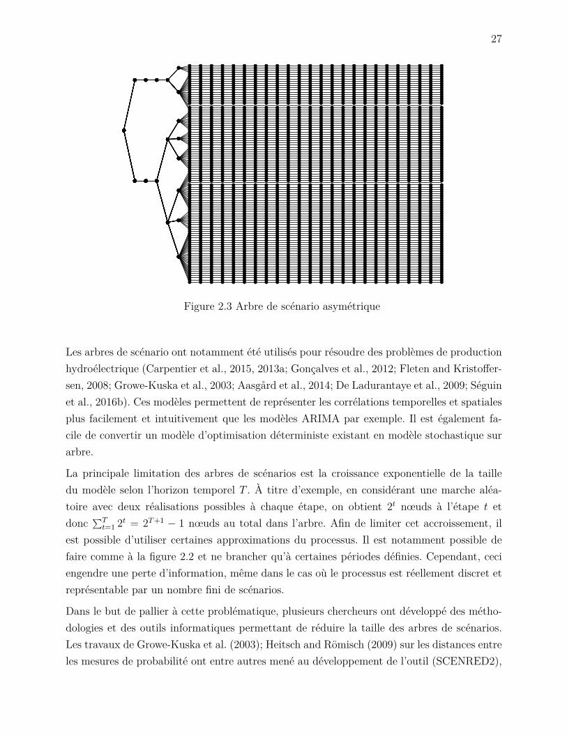
27

Figure 2.3 Arbre de scénario asymétrique

Les arbres de scénario ont notamment été utilisés pour résoudre des problèmes de productionhydroélectrique (Carpentier et al., 2015, 2013a; Gonçalves et al., 2012; Fleten and Kristoffer-sen, 2008; Growe-Kuska et al., 2003; Aasgård et al., 2014; De Ladurantaye et al., 2009; Séguinet al., 2016b). Ces modèles permettent de représenter les corrélations temporelles et spatialesplus facilement et intuitivement que les modèles ARIMA par exemple. Il est également fa-cile de convertir un modèle d’optimisation déterministe existant en modèle stochastique surarbre.

La principale limitation des arbres de scénarios est la croissance exponentielle de la tailledu modèle selon l’horizon temporel T . À titre d’exemple, en considérant une marche aléa-toire avec deux réalisations possibles à chaque étape, on obtient 2t nœuds à l’étape t etdonc ∑T

t=1 2t = 2T+1 − 1 nœuds au total dans l’arbre. Afin de limiter cet accroissement, ilest possible d’utiliser certaines approximations du processus. Il est notamment possible defaire comme à la figure 2.2 et ne brancher qu’à certaines périodes définies. Cependant, ceciengendre une perte d’information, même dans le cas où le processus est réellement discret etreprésentable par un nombre fini de scénarios.

Dans le but de pallier à cette problématique, plusieurs chercheurs ont développé des métho-dologies et des outils informatiques permettant de réduire la taille des arbres de scénarios.Les travaux de Growe-Kuska et al. (2003); Heitsch and Römisch (2009) sur les distances entreles mesures de probabilité ont entre autres mené au développement de l’outil (SCENRED2),

28

intégré à la librairie GAMS. L’outil permet de construire des arbres de scénarios à partir depeignes ou encore de réduire la taille de l’arbre initial et a notamment été utilisées par Fengand Ryan (2014). Les travaux récents de Pflug and Pichler (2016) ont également proposéune approche théorique basée sur les distances de probabilités imbriquées. Ce concept a étéexploité par Séguin et al. (2016b) pour un problème de gestion hydroélectrique court termeréel.

Une approche alternative consiste à utiliser l’algorithme progressive hedging introduit initia-lement par Rockafellar and Wets (1991). Cette technique consiste essentiellement à décom-poser l’arbre en un peigne composé de scénarios indépendants et d’imposer des contraintesde non-anticipativité pour lier certains de ces scénarios. On utilise ensuite une méthode delangrangien augmenté pour pénaliser les violations des contraintes de non-anticipativité.

Cette méthode a été étudiée par Carpentier et al. (2013a) dans le cadre d’une étude surl’évaluation des politiques de gestion des réservoirs au Québec ainsi que par Gonçalves et al.(2012, 2013) pour résoudre le problème de coordination hydro-thermal au Brésil. Toutefois,l’algorithme est sensible aux variations des paramètres et la convergence peut être longueà atteindre. Tel que mentionné brièvement par Côté and Leconte (2015), il est assez lourdd’implémenter le progressive hedging pour des problèmes réels, surtout si on veut évaluer lesrègles de gestion à l’aide de simulation et d’un horizon fuyant.

2.6 Règles de décision linéaires/affines (Linear/affine decision rules) 3

Bien que les méthodes de résolution présentées aux sections précédentes possèdent des avan-tages indéniables et aient été utilisées avec succès pour résoudre des problèmes industrielsréels, elles supposent (presque) toutes que les variables aléatoires suivent une distributiondiscrète.

Cette hypothèse assez forte se révèle parfois problématique, car elle entraîne des difficultésnumériques importantes. Pour les arbres de scénarios, la dimension de l’espace des décisionscroît exponentiellement selon l’horizon du problème. Pour les méthodes liées à la program-mation dynamique, la complexité croît exponentiellement selon la dimension de l’incertitudeet la considération de la corrélation temporelle augmente la taille des variables d’état.

Bien que la méthode SDDP ne nécessite pas de faire l’hypothèse de distributions discrètes, ellenécessite quand même de pouvoir échantillonner à partir de la distribution. De plus, le nombre

3. Dans le reste du texte, on utilise les termes "affine" et "linéaire" de manière interchangeable. En effet,pour une fonction affine l : Rp → Rq de la forme l(ξ) = L0 + L∆ξ où p, q ∈ N, L0 ∈ Rq, L∆ ∈ Rq×p et ξ ∈Ξ ⊂ Rp on peut trouver une fonctions linéaire correspondante l(ξ) = L∆ξ où ξ ∈ (1, ξ>)> : ξ ∈ Ξ ⊂ Rp+1

et L∆ = (L0, L∆) ∈ Rq×(p+1) (voir Georghiou et al. (2015)).

29

de problèmes d’optimisation résolus dépend du nombre de réalisations échantillonnées, autantpour la phase avant que la phase arrière.

La discrétisation de l’incertitude complique également l’implémentation des règles de gestiondans le cas usuel où l’incertitude suit une loi continue. Par exemple, il faut procéder à uneinterpolation des fonctions de valeurs lorsqu’on utilise des méthodes dérivées de la program-mation dynamique, car leur valeur est uniquement calculée explicitement à quelques points.De manière semblable, les arbres de scénarios conduisent à des politiques implémentables 4

uniquement lorsqu’un scénario considéré par le modèle se matérialise réellement.

Bien qu’il soit possible de contourner cette limitation en résolvant ces problèmes en horizonfuyant, cette approche peut se révéler assez lourde en temps de calcul lorsqu’on effectue dessimulations avec de nombreux scénarios d’apport.

Plutôt que de considérer des règles de gestion arbitraires et de les approximer en les discréti-sant comme c’est le cas pour SDP, SSDP et la programmation stochastique sur arbre, il estpossible d’étudier un ensemble limité de fonctions ayant une forme particulièrement simple.Cette thèse utilise notamment les règles de décision linéaires (linear decision rules) et lesrègles de décision linéaires par morceaux aussi connues sous le nom de règles de décision"liftées" (lifted decision rules).

La méthode basée sur ces règles de décision suppose qu’au temps t, on optimise sur un espacede fonctions de la forme Xt : RrT → Rnt où nt ∈ N, r ∈ N et T représentent respectivementla dimension de l’espace des décisions, la dimension de l’incertitude (les apports ξt dans cettethèse) et l’horizon temporel (fini). Si Kt = nt−1 + 1, · · · , nt−1 + nt représente l’ensembledes indices associés aux décisions au temps t et que ξtTt=1 représente les apports où ξt estun vecteur aléatoire de dimension r pour tout t, alors il est possible d’exprimer les règles dedécision linéaires sous la forme :

Xk,t(ξ) = X 0k,t +

r∑j=1

T∑t′=1X t′,ik,t ξt′,j, ∀k ∈ Kt (2.17)

où X 0k,t,X

t′,ik,t ∈ R sont les paramètres de la fonction affine des apports à optimiser. Dans les

cas où E [ξtj] = 0,∀j, t, on peut interpréter X 0k,t comme la décision moyenne ou nominale alors

que le termer∑j=1

T∑t′=1X t′,ik,t ξj,t′ permet d’ajuster cette solution aux différentes réalisations des

4. On définit l’implémentabilité comme le fait de pouvoir mettre en application une décision réelle etpertinente (par exemple la quantité de débits à soutirer d’un réservoir) uniquement sur la base de l’informationdisponible à ce moment.

30

ξjt.

Afin d’obtenir des règles de décision implémentables 5, on impose X t′,ik,t = 0,∀t′ ≥ t,∀i =

1, · · · , r. Ceci permet naturellement de s’assurer que les décisions à prendre au temps tdépendent uniquement de ξ[t−1], l’historique des apports observés.

Dans le reste de cette section ainsi que le reste de la thèse, on considère le cas particulier r = 1.Il est notamment raisonnable de supposer que le processus d’apports est unidimensionel sion considère une seul réservoir ou si on étudie les apports sur toute la rivière.

Il est surprenant de constater que les règles de décision linéaires ont été introduites il y aplus de 40 ans pour optimiser la capacité de réservoirs multi-usage sous certaines contraintessur la navigation et le risque d’inondation (ReVelle and Kirby, 1970; Loucks and Dorfman,1975). Ces auteurs considèrent par exemple le cas où les débits soutirés prennent la forme :

Rt = St − Bt (2.18)

où Rt,St représentent respectivement les débits soutirés, les volumes d’eau dans le réservoirau temps t et Bt est une variable de décision réelle à optimiser. En négligeant les débitsdéversés, les contraintes de conservation de l’eau s’expriment comme : St+1 = St + ξt−Rt oùξt sont les apports. En exploitant (2.18) et en explicitant la dépendance sur ξt, on a donc :

St+1(ξ) = ξt + Bt, t = 1, · · · , T (2.19)Rt+1(ξ) = ξt + Bt − Bt+1, t = 1, · · · , T (2.20)S1(ξ) = S1, (2.21)R1(ξ) = S1 − B1, (2.22)

où l’on suppose que S1 est connu. S1(·) et R1(·) sont donc des fonctions constantes del’incertitude.

On peut donc conclure que sous cette forme, les volumes et les débits soutirés sont biendes fonctions affines de l’incertitude ayant la forme (2.17). Cependant, ils représentent uncas relativement limitant et rigide, car les Bt sont communs à St+1 et Rt+1 et on fixe lecoefficients de ξt à 1 et celui de ξt−l à 0 pour l = 1, · · · , t − 1. Les débits et les volumes

5. On dit également que les règles de décision sont causales, non anticipatives ou encore adaptées à lafiltration FtTt=1 où Ft = σ(ξ[t−1]) représente l’information contenue par l’historique ξ[t−1].

31

au temps t dépendent donc uniquement des apports à ce temps donné d’une manière trèsprécise.

Une autre limitation importante de ces travaux est le fait de supposer que les apports suiventune distribution particulière connue parfaitement. Sous cette hypothèse, ces auteurs par-viennent à modéliser le problème comme un problème avec contraintes probabilistes (chance-constrained problem). Ils garantissent ainsi que les contraintes du type Rt(ξ) ≤ r sont res-pectées avec une probabilité 1− ε pour un petit ε > 0 fixé.

Certains auteurs comme Stedinger (1984) ont néanmoins critiqué l’utilisation pratique detels modèles, notamment car ils conduisent à des décisions trop rigides se révélant souventtrop conservatrices lorsqu’évaluées sur des scénarios réels. Les règles de décision linéaires ontdonc perdu beaucoup de popularité au cours des décennies suivantes.

Il a fallu attendre les années 2000 avant que les travaux de Ben-Tal et al. (2004) et Kuhn et al.(2011) sur les problèmes stochastiques et robustes 6multi-étapes redonnent une impulsion auxrègles de décision linéaires. 7 Depuis cette période, les règles de décision linéaires ont connu unregain d’intérêt considérable. Bertsimas et al. (2010) ont étudié leurs propriétés et ont établicertaines conditions garantissant leur optimalité. Kuhn et al. (2011) proposent d’utiliser cesrègles de décision sur le problème dual et primal afin de pouvoir évaluer leur degré de sous-optimalité. Afin d’améliorer leur performance, plusieurs auteurs ont également développé desextensions afin de considérer des règles de décision linéaires sur un espace lifté (Georghiouet al., 2015; Goh and Sim, 2010) ou encore des règles de décision entières (Bertsimas andGeorghiou, 2015).

Les règles de décision linéaires ont également été utilisées avec succès dans de nombreuxdomaines comme la gestion d’inventaires, la localisation d’entrepôts, la gestion de projets, etc.(Delage and Iancu). Ces techniques ont également été exploitées pour résoudre des problèmesen énergie comme les problèmes de chargement (unit commitment problems) (Lorca and Sun,2015; Lorca et al., 2016; Bertsimas et al., 2013) et des problèmes de gestion de portefeuille

7. On définit l’optimisation robuste comme une méthodologie de prise de décision en présence d’incertitudefaisant un nombre minimal d’hypothèses sur l’aléa et axée sur la tractabilité des problèmes résolus (Ben-Talet al., 2009). Un problème d’optimisation robuste est habituellement formulé comme un problème de laforme : minx∈X maxξ∈Ξf(x, ξ) : gi(x, ξ) ≤ 0, ∀i = 1, · · · ,m,∀ξ ∈ Ξ où X et Ξ représentent des ensemblesdéterministes convexes et f(·, ·) et gi(·, ·) sont des fonctions convexes en x et concave en ξ. On supposeégalement couramment que le problème de maximisation interne puisse se formuler comme un programmelinéaire, conique de second ordre ou semi-défini afin de pouvoir utiliser la dualité pour le reformuler comme unproblème de minimisation. L’approche peut s’inscrire dans un cadre non-probabiliste ou probabiliste, commec’est le cas dans ce mémoire. Dans ce second cas, on suppose que l’aléa (ξ) peut être représenté par desvariables aléatoires dont on connait certaines informations comme le support et l’espérance. L’optimisationrobuste probabiliste peut donc être considérée comme une branche de l’optimisation stochastique.

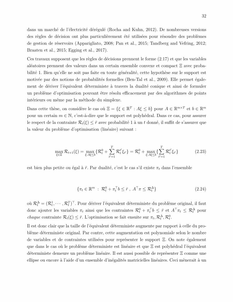
32

dans un marché de l’électricité dérégulé (Rocha and Kuhn, 2012). De nombreuses versionsdes règles de décision ont plus particulièrement été utilisées pour résoudre des problèmesde gestion de réservoirs (Apparigliato, 2008; Pan et al., 2015; Tandberg and Vefring, 2012;Braaten et al., 2015; Egging et al., 2017).

Ces travaux supposent que les règles de décisions prennent le forme (2.17) et que les variablesaléatoires prennent des valeurs dans un certain ensemble convexe et compact Ξ avec proba-bilité 1. Bien qu’elle ne soit pas faite en toute généralité, cette hypothèse sur le support estmotivée par des notions de probabilités formelles (Ben-Tal et al., 2009). Elle permet égale-ment de dériver l’équivalent déterministe à travers la dualité conique et ainsi de formulerun problème d’optimisation pouvant être résolu efficacement par des algorithmes de pointsintérieurs ou même par la méthode du simplexe.

Dans cette thèse, on considère le cas où Ξ = ξ ∈ RT : Aξ ≤ b pour A ∈ Rm×T et b ∈ Rm

pour un certain m ∈ N, c’est-à-dire que le support est polyhédral. Dans ce cas, pour assurerle respect de la contrainte Rt(ξ) ≤ r avec probabilité 1 à un t donné, il suffit de s’assurer quela valeur du problème d’optimisation (linéaire) suivant :

maxξ∈ΞRt+1(ξ) = max

ξ:Aξ≤bR0

t +T∑t′=1Rt′

t ξt′ = R0t + max

ξ:Aξ≤b

T∑t′=1Rt′

t ξt′ (2.23)

est bien plus petite ou égal à r. Par dualité, c’est le cas s’il existe πt dans l’ensemble

πt ∈ Rm : R0t + π>t b ≤ r , A>π ≤ R∆

t (2.24)

où R∆t = (R1

t , · · · ,RTt )>. Pour dériver l’équivalent déterministe du problème original, il faut

donc ajouter les variables πt ainsi que les contraintes R0t + π>t b ≤ r et A>πt ≤ R∆

t pourchaque contrainte Rt(ξ) ≤ r. L’optimisation se fait ensuite sur πt,R∆

t ,R0t .

Il est donc clair que la taille de l’équivalent déterministe augmente par rapport à celle du pro-blème déterministe original. Par contre, cette augmentation est polynomiale selon le nombrede variables et de contraintes utilisées pour représenter le support Ξ. On note égalementque dans le cas où le problème déterministe est linéaire et que Ξ est polyhédral l’équivalentdéterministe demeure un problème linéaire. Il est aussi possible de représenter Ξ comme uneellipse ou encore à l’aide d’un ensemble d’inégalités matricielles linéaires. Ceci mènerait à un

33

problème conique de second ordre ou un problème semi-défini.

2.6.1 Mesures de risque

Dans la grande majorité des travaux cités aux sections précédentes, l’objectif à optimiser estla valeur espérée d’une fonction de récompense, typiquement une combinaison linéaire de laproduction hydroélectrique totale, de pénalisations pour des violations de contraintes et/oude déversés ainsi qu’une valorisation du stock final d’eau.

Bien que l’espérance mathématique et l’espérance conditionnelle possèdent des avantagesconsidérables comme la linéarité et la propriété de l’espérance totale en plus d’être bien étu-diées, ces fonctionnelles souffrent également de limitations importantes. On considère souventl’espérance dans une optique intuitive où l’on cherche à s’assurer de la performance d’unsystème en moyenne sur un grand nombre de réalisations. Cependant, tel que soulevé parBen-Tal et al. (2009), cette interprétation par la loi des grands nombres est uniquement sa-tisfaisante pour un preneur de décision si ce dernier est prêt à échantillonner de nombreusesobservations 8.

Une telle hypothèse est peut-être vérifiée dans le cas de la production hydroélectrique courtterme où la planification doit être effectuée de très nombreuses fois. Dans ce cas, il est proba-blement acceptable de produire moins durant certains jours si cette réduction est compenséepar une production accrue pendant une autre période. Toutefois, ce n’est pas nécessairementle cas pour la minimisation d’inondations, car les conséquences humaines et environnemen-tales d’une seule occurrence d’un tel désastre sont extrêmement importantes.

Afin de modéliser cette aversion au risque, il est possible d’utiliser les travaux importants surla théorie de l’utilité espérée (Neumann and Morgenstern, 1953; Föllmer and Schied, 2011).Toutefois, il est souvent difficile de bien codifier la fonction d’utilité pour un preneur dedécision particulier (Armbruster and Delage, 2015). Par ailleurs, plusieurs travaux suggèrentque les fonctions d’utilité seraient non convexes et non concaves en réalité, ce qui mènerait àdes difficultés numériques considérables. Les lacunes de la théorie de l’utilité espérée ont par

7. Il existe des similitudes très marquées entre l’histoire des règles de décision linéaires et celle de l’opti-misation robuste. En effet, l’optimisation robuste a initialement été introduite dans les années 70 par Soyster(1973) pour résoudre des problèmes linéaires incertains. Toutefois, cette méthodologie est uniquement deve-nue populaire dans les années 2000 suite notamment aux développements en optimisation conique (Ben-Taland Nemirovski, 1998; El Ghaoui and Lebret, 1997; El Ghaoui et al., 1998). Ces recherches ont a leur tourgénéré de l’attention sur les problèmes avec incertitude linéaire (Sim and Bertsimas, 2004) et ont même menéau développement d’outils de formulation automatiques (Goh and Sim, 2011). Ces avancées ont grandementfacilité l’utilisation et la popularité de la méthodologie.

8. Si ces observations sont faites à travers le temps, alors ce système doit également se comporter de façonstationnaire.

34

ailleurs mené à la formulation de paradoxes comme celui d’Ellsberg (Ellsberg, 1961). 9

Le paradoxe d’Ellsberg est intéressant, car il démontre que la plupart des individus ne res-pectent pas les axiomes classiques de la théorie de l’utilité espérée. Ces derniers font plutôtpreuve d’aversion à l’ambiguïté. En effet, ils font face non seulement à de l’incertitude auniveau des réalisations des variables aléatoires, mais également à une ambiguïté sur la distri-bution à considérer. En d’autres mots, il existe un risque sur le risque.

Les travaux de Artzner et al. (1999) sur la théorie des mesures de risque cohérentes per-mettent de répondre à certaines de ces critiques. Cette approche consiste à définir un en-semble de fonctionnelles possédant certaines propriétés computationelles désirables fondéessur des axiomes intuitifs et rigoureux.

Si on considère U,W ∈ L∞ où L∞ est un espace de variables aléatoires bornées avec pro-babilité 1, alors on définit une mesure de risque comme une fonctionnelle ρ : L∞ → R tellequ’une position aléatoire U est acceptable si ρ(U) ≤ 0, c’est-à-dire si le risque ρ(U) de lavariable aléatoire U est non positif. On cherche à minimiser ρ(U) et on peut donc interpréterU comme une perte ou une violation. Les mesures de risque cohérentes respectent les quatreaxiomes suivant :

U ≥ W ⇒ ρ(U) ≥ ρ(W ), (2.25)ρ(U + c) = ρ(U) + c,∀c ∈ R, (2.26)ρ(λU + (1− λ)W ) ≤ λρ(U) + (1− λ)ρ(W ),∀λ ∈ [0, 1], (2.27)ρ(λU) = λρ(U),∀λ ≥ 0, (2.28)

où l’inégalité U ≥ W tient avec probabilité 1 et c et λ sont des constantes réelles.

9. Le paradoxe d’Ellsberg est illustré à l’aide d’une expérience assez simple. On considère une urne remplied’un tiers de balles rouges et de deux tiers de balles jaunes et noires dont on ignore les proportions exactes.On considère ensuite 2 rondes où l’on propose chaque fois 2 paris à une personne. Au cours de la premièreronde, on offre le choix entre A : 100 $ si une balle rouge est tirée et B : 100 $ si une balle noire est tirée.Pendant la deuxième ronde, on propose ensuite C : 100 $ si on tire une balle jaune ou rouge et D : 100 $si on tire une balle jaune ou noire. selon la théorie de l’utilité espérée, une personne rationnelle qui préfèrestrictement (n’est pas indifférente) le choix A estime que la proportion de balles rouges est supérieure à cellede balles noires. Ainsi, pour être cohérente avec son premier choix, cette personne devrait également préférerstrictement le choix C au choix D. Hors, en pratique, les participants préfèrent majoritairement le choix Apar rapport au B ainsi que le choix D par rapport au C. Cette contradiction apparente découle possiblementdu fait que l’on sait exactement que la probabilité de gagner les paris A et D est de 1

3 et 23 , respectivement,

alors que la probabilité de gagner les paris B et C se situe dans les intervalles [0, 23 ] et [ 1

3 , 1], respectivement.En d’autres termes, il existe de l’ambiguïté sur les paris B et C et la pire probabilité de B ou C est inférieureà la probabilité certaine du pari correspondant.

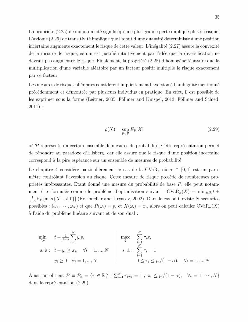
35

La propriété (2.25) de monotonicité signifie qu’une plus grande perte implique plus de risque.L’axiome (2.26) de transitivité implique que l’ajout d’une quantité déterministe à une positionincertaine augmente exactement le risque de cette valeur. L’inégalité (2.27) assure la convexitéde la mesure de risque, ce qui est justifié intuitivement par l’idée que la diversification nedevrait pas augmenter le risque. Finalement, la propriété (2.28) d’homogénéité assure que lamultiplication d’une variable aléatoire par un facteur positif multiplie le risque exactementpar ce facteur.

Les mesures de risque cohérentes considèrent implicitement l’aversion à l’ambiguïté mentionnéprécédemment et démontrée par plusieurs individus en pratique. En effet, il est possible deles exprimer sous la forme (Leitner, 2005; Föllmer and Knispel, 2013; Föllmer and Schied,2011) :

ρ(X) = supP∈P

EP [X] (2.29)

où P représente un certain ensemble de mesures de probabilité. Cette représentation permetde répondre au paradoxe d’Ellsberg, car elle assure que le risque d’une position incertainecorrespond à la pire espérance sur un ensemble de mesures de probabilité.

Le chapitre 4 considère particulièrement le cas de la CVaRα où α ∈ [0, 1] est un para-mètre contrôlant l’aversion au risque. Cette mesure de risque possède de nombreuses pro-priétés intéressantes. Étant donné une mesure du probabilité de base P , elle peut notam-ment être formulée comme le problème d’optimisation suivant : CVaRα(X) = mint∈R t +

11−αEP [maxX − t, 0] (Rockafellar and Uryasev, 2002). Dans le cas où il existe N scénariospossibles : (ω1, · · · , ωN) et que P (ωi) = pi et X(ωi) = xi, alors on peut calculer CVaRα(X)à l’aide du problème linéaire suivant et de son dual :

mint,y

t+ 11−α

N∑i=1

yipi maxq

N∑i=1

πixi

s. à : t+ yi ≥ xi, ∀i = 1, ..., N s. à :N∑i=1

πi = 1

yi ≥ 0 ∀i = 1, ..., N 0 ≤ πi ≤ pi/(1− α), ∀i = 1, ..., N

Ainsi, on obtient P ≡ Pα = π ∈ RN+ : ∑N

i=1 πixi = 1 ; πi ≤ pi/(1 − α), ∀i = 1, · · · , Ndans la représentation (2.29).

36

On peut également écrire CVaRα(X) = 11−α

∫ 1α qX(t)dt où qX(α) = inft : FX(t) ≥ α est la

fonction de quantile évaluée en α ∈ (0, 1). La fonction qX(·) est la pseudo-inverse de la fonctionde répartition FX(·) où FX(x) = P (X ≤ x) pour x ∈ R (Acerbi and Tasche, 2002). Dans lecas où FX est continue, on obtient donc CVaRα(X) = 1

1−αE[XIX>qX(α)

]= E [X|X > qX(α)]

Cette interprétation à l’aide de l’espérance conditionnelle est intéressante, car elle indique in-tuitivement que l’on considère uniquement les pires 100(1−α) % des scénarios. Par ailleurs,on peut démontrer que E [X] ≤ CVaRα(X) ≤ ess sup X pour tout α ∈ (0, 1) ainsi quelimα→0 CVaRα(X) = E [X] et limα→1 CVaRα(X) = ess sup X où ess sup X indique la plusgrande valeur (le supremum) que X peut prendre avec probabilité 1. Le paramètre α repré-sente donc une manière simple et efficace de contrôler l’aversion au risque.

Les mesures de risque ont gagné en popularité au cours des dernières années. Bien qu’ellesaient initialement été appliquées au domaine financier, notamment pour évaluer le risquede crédit et gérer des portefeuille (Acerbi and Tasche, 2002; Bertsimas et al., 2004), ellesont trouvé de nombreuses applications pratiques et théoriques en recherche opérationnelle(Chen et al., 2010; Natarajan et al., 2009; Brown and Bertsimas, 2009; Brown, 2007), plusspécifiquement en optimisation de la production énergétique (Gonçalves et al., 2013; Shapiroet al., 2013).

37

CHAPITRE 3 ORGANISATION DE LA THÈSE

Les trois prochains chapitres sont associés à trois article publiés ou soumis dans des revuesscientifiques. Ces travaux considèrent tous le problème de gestion de réservoir court terme enprésence d’incertitude. On s’intéresse plus particulièrement à la gestion mensuelle de la rivièreGatineau avec pas de temps journaliers. L’accent est mis sur les nombreuses contraintes opé-rationnelles spécifiques au bassin versant comme le risque d’inondations à différents segmentsde la rivière.

Les modèles et les algorithmes ont été développés dans le but de produire un outil d’aide à ladécision permettant de faciliter le travail des gestionnaires de la rivière. À cet effet, tous lesmodèles sont relativement faciles à implémenter, permettent d’obtenir de bonnes solutionstrès rapidement et peuvent être utilisés dans un contexte de simulation pour procéder à desétudes de cas.

Le chapitre 4 s’intéresse à la minimisation du risque d’inondations. Après avoir introduit leproblème de gestion de réservoir, on propose une modélisation du problème déterministe.On introduit ensuite les règles de décision linéaires et les règles liftées. Ceci nous permet deformuler l’équivalent déterministe comme un problème linéaire qu’on résout avec CPLEX.

Le chapitre présente également une étude numérique assez exhaustive basée sur diversessimulations et règles de gestion. On s’intéresse notamment à la résolution d’un modèle dé-terministe en horizon roulant, un modèle de programmation stochastique sur arbre construitavec SCENRED2, quelques variantes des règles de décision affines ainsi que les règles de dé-cision liftées. Le chapitre conclut qu’en général, les règles de décision affines qui considèrentuniquement l’incertitude sur un horizon limité offrent les meilleurs compromis entre tempsde calcul et performance.

On y étudie aussi la performance de quelques représentations polyhédrales utilisées couram-ment dans la littérature sous l’influence de différents processus hydrologiques. On expliquenotamment qu’en présence de forte corrélation temporelle, il peut être néfaste d’utiliser unensemble basé sur un budget d’incertitude (Sim and Bertsimas, 2004) trop petit.

Finalement, cet article analyse l’impact de l’utilisation de la mesure de risque CVaRα avecdifférentes tolérances α ∈ [0, 1]. Les résultats de simulation n’apportent pas de conclusionprobante applicable à tous les modèles. Ceci est peut-être dû au fait que les simulationsconsidèrent des réalisations de l’incertitude plus réalistes que le modèle d’optimisation. Cettesimulation hors-échantillon mène à des conditions pour lesquelles le modèle d’optimisation

38

n’a pas été calibré.

Le chapitre 5 jette les bases de l’utilisation de séries chronologiques de type ARIMA pour desproblèmes stochastiques multi-étapes avec règles de décision. On considère initialement unprocessus ARMA(1,1) stationnaire où les chocs sont indépendants, mais on étend les travauxau cas où ils sont uniquement non corrélés et suivent un processus GARCH(1,1). On supposeici que les apports sont une fonction linéaire des chocs et que ces derniers appartiennent àun polyhèdre motivé par l’inégalité de Chebychev.

Contrairement au chapitre 4, on minimise une fonction quadratique convexe des inondationsafin de refléter les conséquences marginales croissantes des inondations. Ceci mène à unproblème quadratique où l’objectif varie dans le temps selon les réalisations passées lorsqu’onajoute l’hétéroscédasticité.

Bien que les résultats de simulation soient prometteurs, cette section ne semble pas indiquerun avantage important d’une modélisation basée sur les processus ARMA par rapport à unereprésentation ignorant la corrélation temporelle similaire à celle utilisée dans le chapitre 4dans le cas des apports historiques. Effectivement, les modèles GARCH(1,1) + ARMA(1,1),ARMA(1,1) ainsi que le modèle naïf donnent des performances semblables en termes deminimisation des inondations. Cette faiblesse est attribuable au choix de modèle ARMAlinéaire qui viole certaines propriétés de base comme la non-négativité des apports en plusd’offrir un potentiel prédictif faible.

Contrairement aux deux premiers chapitres 4 et 5, le chapitre 6 considère également la valo-risation du stock d’eau, la production hydroélectrique ainsi que le risque d’inondations. Onconsidère une combinaison convexe des différents objectifs et on explore l’espace des solutionsselon différents scénarios hydrologiques.

Afin de modéliser réalistement la production hydroélectrique, on considère une hauteur dechute variable, ce qui mène à un problème non convexe qu’on résout approximativement àl’aide d’un algorithme de région de confiance très simple, mais efficace.

Ce chapitre présente par ailleurs un processus ARMA qui lie les apports aux chocs de façonnon linéaire. Cette représentation plus réaliste mène à un ensemble d’incertitude non convexe,qu’on choisit d’approximer de façon conservatrice par un polyhèdre. Cette forme permetégalement de dériver une expression analytique pour l’espérance conditionnelle.

La section 8 effectue un retour sommaire sur l’ensemble du travail réalisé et propose quelquespistes d’améliorations et de réflexions. On évalue notamment les différentes façons d’améliorerla modélisation de la rivière et des apports.

39

CHAPITRE 4 ARTICLE 1: DECISION RULE APPROXIMATIONS FORTHE RISK AVERSE RESERVOIR MANGEMENT PROBLEM

Cet article a été publié : Gauvin, C., Delage, E., and Gendreau, M. (2017). Decision ruleapproximations for the risk averse reservoir management problem. European Journal ofOperational Research, 261 :317–336. (Gauvin et al., 2017). 1Auteurs : Charles Gauvin, ErickDelage et Michel Gendreau.

Abstract : This paper presents a new formulation for the risk averse stochastic reservoirmanagement problem. Using recent advances in robust optimization and stochastic program-ming, we propose a multi-stage model based on minimization of a risk measure associatedwith floods and droughts for a hydro-electrical complex. We present our model and thenidentify approximate solutions using standard affine decision rules commonly found in theliterature as well as lifted decision rules. Finally, we conduct thorough numerical experimentsbased on a real river system in Western Québec and conclude on the relative performance offamilies of decision rules.

Keywords : Stochastic programming, Robust optimization, Risk analysis, OR in energy

4.1 Introduction

The problem of designing an optimal release schedule for a set of interconnected reservoirsis extremely challenging. Operators must often make decisions for various dams or otherwater control structures in each period of a given time horizon while taking into accountthe dynamical structure and topology of the system. It may also be important to considercomplex non-linear physical phenomenon such as the effect of water volumes on outflow orwater delays. This generally leads to high dimensional dynamic and non-convex problems.

Furthermore, operators must deal with various conflicting objectives of varying importance.Hydro-electrical complexes must namely balance criteria such as recreational and environ-mental needs with electricity generation, irrigation and flood control (Labadie, 2004). The

1. L’écriture de ce chapitre a été légèrement modifiée par rapport au rapport technique afin de standardiserla notation pour l’ensemble de la thèse. Après avoir reçu les rapports d’arbitres pour le deuxième article,nous avons effectué plusieurs changements de notation pour se rapprocher de l’écriture standard en gestion deressources hydriques. Ces changements ne nous avaient pas été demandés pour le premier manuscrit soumisprécédemment à European Journal of Operational Research.

40

importance of considering multiple criteria in stochastic reservoir management problems isnamely illustrated in Hajkowicz and Higgins (2008); Tilmant and Kelman (2007); Castellettiet al. (2010).

Considerable uncertainty surrounds various factors such as price of electricity, turbine brea-kage, inflows and demand. It is virtually impossible to perfectly identify and represent thetrue multi-dimensional stochastic process. However, failure to take into account this stochas-ticity can lead not only to severely suboptimal solutions, but even disastrous consequencessuch as floods or droughts. Incorporating uncertainty also poses serious numerical limitationsas this leads to multi-stage stochastic programs, which are generally intractable (see Dyerand Stougie (2006)).

There is a need to develop scalable and flexible operational tools that can take this uncertaintyinto account. In Québec for instance, current operating practices for short-term planninginclude use of simplified linear programming models or more complex heuristics. Althoughboth approaches evaluate policies on extensive test-beds in order to assess their performanceunder various inflow scenarios, they do not consider stochasticity explicitly.

Existing methods capable of handling decision under uncertainty suffer from various limita-tions. Stochastic dynamic programming (SDP), which has historically been one of the mostpopular algorithms in academia and in practice for reservoir management (Saad and Turgeon,1988; Saad et al., 1996; Turgeon and Charbonneau, 1998; Stedinger and Faber, 2001), cantypically only be applied for problems that ignore water flow delays and consider a limitednumber of reservoirs, typically 1 or 2. In contrast, our case study considers 5 reservoirs andwould require using a state of dimension 18 when considering the sum of past releases over allpossible water delays. The discretization required by SDP may also lead to approximationsand numerical difficulties. Finally, the algorithms often assume normally or log-normally dis-tributed random variables (Turgeon, 2005), which is not verified empirically for daily inflows.

In the last decades, the stochastic dual dynamic programming algorithm (SDDP) (Pereiraand Pinto, 1991; Tilmant and Kelman, 2007; Rougé and Tilmant, 2016) has emerged as viablealternative to traditional SDP to tackle multidimensional problems. This algorithm consistsof a backward recursive phase where the future value function is approximated with Benderscuts though the solution of a dual problem and a forward sampling and simulation phase.This alleviates the curses of dimensionality associated to the space of controls and is thereforeuseful for large reservoir systems. However, the algorithm does not provide implementablepolicies as would an SDP algorithm, can display relatively slow convergence and relies on afixed sampling distribution such as the log-normal Shapiro et al. (2013).

Stochastic programming models based on scenario trees have also attracted attention (Gon-

41

çalves et al., 2012; Carpentier et al., 2013a; Aasgård et al., 2014). This tree representationis useful to model a wide range of distributions while capturing complex correlations ofthe multi-dimensional processes. However, it also fails to provide an implementable policyand generally leads to very large deterministic equivalent programs. In order to mitigate thiscomputational issue, various tree-reduction approaches based on Heitsch and Römisch (2009)have been used. Although useful, the loss of information caused by the aggregation may failto capture more extreme scenarios, which may be essential for flood management purposes.Other scenario aggregation and partitioning schemes (Carpentier et al., 2013b) as well as theprogressive hedging algorithm (Rockafellar and Wets, 1991) have also been investigated. No-netheless, convergence may be long to reach for large problems and these algorithm displaysensitivity to parameters and scenario representation (Carpentier et al., 2013a; Gonçalveset al., 2012).

This paper addresses these issues by proposing a multi-stage multi-reservoir model based onrobust optimization. Robust optimization is a rapidly expanding paradigm that has gainedin popularity over the years (Bertsimas et al., 2011; Ben-Tal et al., 2009). By restrictinguncertainty to reside within a given parametrized and deterministic convex set, large sto-chastic models can be converted into their robust counterparts while maintaining tractabilitythrough conic programming duality.

The robust optimization paradigm has been extended to dynamic problems with affine de-cision rules (Ben-Tal et al., 2004) as well as more sophisticated decision rules by variousauthors to provide more flexibility and precision (Chen et al., 2008; Goh and Sim, 2010;Georghiou et al., 2015). Some of these robust optimization methods have recently been usedfor reservoir management problems. The authors of Apparigliato (2008) and Pan et al. (2015)namely use this framework to derive operating policies to maximize the expected electric pro-duction for a multi-period and multi-reservoir hydro-electric complex. Both works considerlow-dimensional systems of up to 3 reservoirs. They focus on systems where the risk of floodsare relatively modest and therefore only consider bounds on total releases and volumes.

This paper differs significantly from the previous work in that it considers more realisticoperating conditions. Our model explicitly considers water delays, non-linear functions relatedto the physical structure of the evacuation structures and flow variation constraints. Moreover,we focus on a difficult problem instance without complete recourse with tight constraints thatmay be significantly violated under certain inflow scenarios.

For this reason, we formulate a novel multi-dimensional problem that minimizes the riskof floods at various critical locations on the river. Unlike Pan et al. (2015), we do not useover-the-shelf software like ROME (Robust Optimization Made Easy) (Goh and Sim, 2011),

42

because of the computational overhead and because our approach can be tailored to ourspecific needs. This is namely important because the built-in lifted decision rules cannot beadapted to the ones used in this paper to the best of our knowledge.

Unlike competing methods like SDP, SDDP and stochastic programs based on scenario trees,robust optimization reduces the need for distributional assumptions. In particular, it does notrequire fixing a pre-specified distribution from which it is possible to sample. As observed byPan et al. (2015), this increases the resilience of the solutions when tested on out-of-sampledata while providing similar performance for in-sample data.

Although these decision rules provide a conservative approximation of the objective value,they remain tractable and provide rules that can easily be used in simulations, which is notnecessarily the case of SDDP or tree-based stochastic programs, except when used in a rollinghorizon fashion. The ability to simulate river management policies is of prime importance forpractical reservoir management. Difficulty to evaluate solutions based on multi-stage decisiontrees has namely impeded their implementation in practice.

Contrary to an overwhelming majority of models mentioned previously, including Appari-gliato (2008) and Pan et al. (2015), we do not assume risk neutrality. We explicitly considerrisk aversion and perform sensitivity analysis on the α parameter of the coherent risk mea-sure CVaRα. This allows us to easily interpret the risk of these natural disasters and performsensitivity analysis.

Like Pan et al. (2015), we evaluate the use of linear and piecewise affine decision rules. Ourwork draws heavily from both state-of-the art techniques in robust optimization and thework of Georghiou et al. (2015) on stochastic programming. We conduct extensive numericalexperiments based on a real river system to evaluate and compare these different policies andalso consider a rolling horizon approach embedded in a realistic simulation environment.

The rest of the paper is structured as follows. We introduce our deterministic model andthe objective in Section 4.2. Section 4.3 focuses on the uncertainty surrounding inflows whilesection 4.4 discusses risk analysis. Section 4.5 discusses affine and piecewise-affine decisionrules. We then present a case study based on a real hydroelectric reservoir managementproblem in Québec in Section 4.6 and offer concluding remarks in Section 4.7.

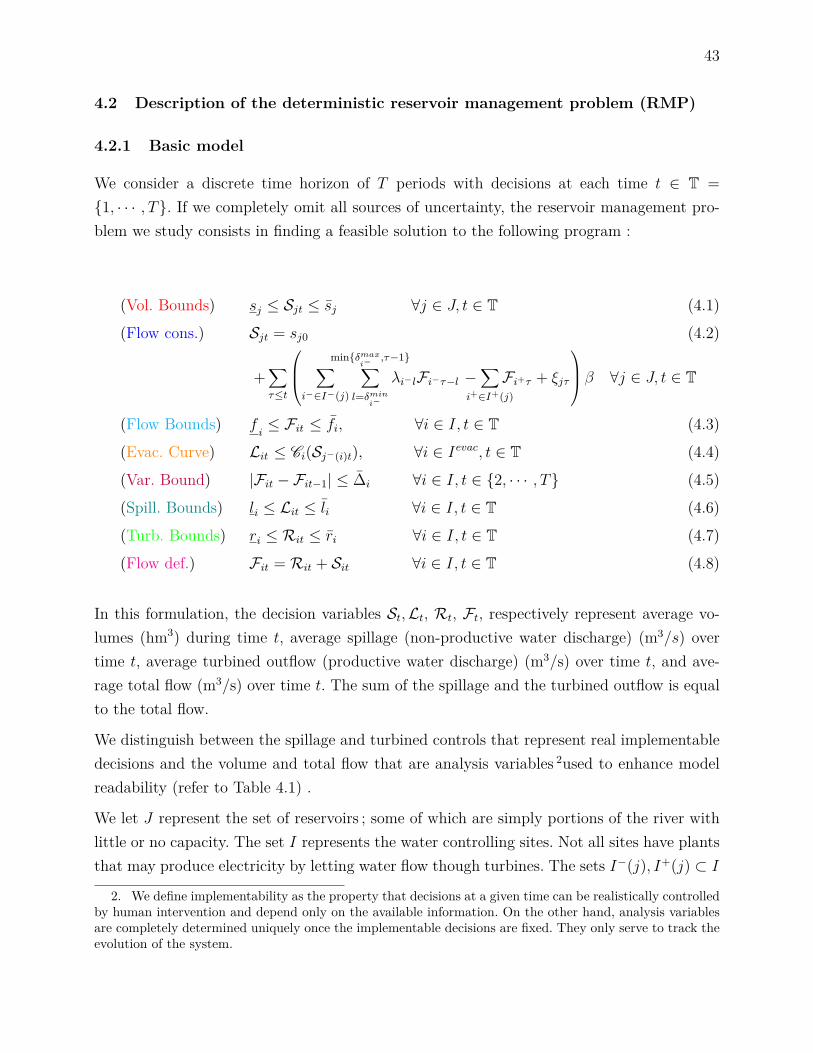
43

4.2 Description of the deterministic reservoir management problem (RMP)

4.2.1 Basic model

We consider a discrete time horizon of T periods with decisions at each time t ∈ T =1, · · · , T. If we completely omit all sources of uncertainty, the reservoir management pro-blem we study consists in finding a feasible solution to the following program :

(Vol. Bounds) sj ≤ Sjt ≤ sj ∀j ∈ J, t ∈ T (4.1)(Flow cons.) Sjt = sj0 (4.2)

+∑τ≤t

∑i−∈I−(j)

minδmaxi−

,τ−1∑l=δmin

i−

λi−lFi−τ−l −∑

i+∈I+(j)Fi+τ + ξjτ

β ∀j ∈ J, t ∈ T

(Flow Bounds) fi≤ Fit ≤ fi, ∀i ∈ I, t ∈ T (4.3)

(Evac. Curve) Lit ≤ Ci(Sj−(i)t), ∀i ∈ Ievac, t ∈ T (4.4)(Var. Bound) |Fit −Fit−1| ≤ ∆i ∀i ∈ I, t ∈ 2, · · · , T (4.5)(Spill. Bounds) li ≤ Lit ≤ li ∀i ∈ I, t ∈ T (4.6)(Turb. Bounds) ri ≤ Rit ≤ ri ∀i ∈ I, t ∈ T (4.7)(Flow def.) Fit = Rit + Sit ∀i ∈ I, t ∈ T (4.8)

In this formulation, the decision variables St,Lt, Rt, Ft, respectively represent average vo-lumes (hm3) during time t, average spillage (non-productive water discharge) (m3/s) overtime t, average turbined outflow (productive water discharge) (m3/s) over time t, and ave-rage total flow (m3/s) over time t. The sum of the spillage and the turbined outflow is equalto the total flow.

We distinguish between the spillage and turbined controls that represent real implementabledecisions and the volume and total flow that are analysis variables 2used to enhance modelreadability (refer to Table 4.1) .

We let J represent the set of reservoirs ; some of which are simply portions of the river withlittle or no capacity. The set I represents the water controlling sites. Not all sites have plantsthat may produce electricity by letting water flow though turbines. The sets I−(j), I+(j) ⊂ I

2. We define implementability as the property that decisions at a given time can be realistically controlledby human intervention and depend only on the available information. On the other hand, analysis variablesare completely determined uniquely once the implementable decisions are fixed. They only serve to track theevolution of the system.

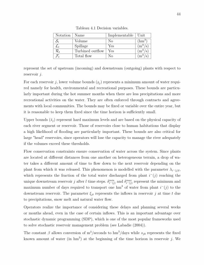
44

Tableau 4.1 Decision variables.

Notation Name Implementable UnitSt Volume No (hm3)Lt Spillage Yes (m3/s)Rt Turbined outflow Yes (m3/s)Ft Total flow No (m3/s)

represent the set of upstream (incoming) and downstream (outgoing) plants with respect toreservoir j.

For each reservoir j, lower volume bounds (sj) represents a minimum amount of water requi-red namely for health, environmental and recreational purposes. These bounds are particu-larly important during the hot summer months when there are less precipitations and morerecreational activities on the water. They are often enforced through contracts and agree-ments with local communities. The bounds may be fixed or variable over the entire year, butit is reasonable to keep them fixed since the time horizon is sufficiently small.

Upper bounds (sj) represent hard maximum levels and are based on the physical capacity ofeach river segment or reservoir. Those of reservoirs close to human habitations that displaya high likelihood of flooding are particularly important. These bounds are also critical forlarge "head" reservoirs, since operators will lose the capacity to manage the river adequatelyif the volumes exceed these thresholds.

Flow conservation constraints ensure conservation of water across the system. Since plantsare located at different distances from one another on heterogeneous terrain, a drop of wa-ter takes a different amount of time to flow down to the next reservoir depending on theplant from which it was released. This phenomenon is modelled with the parameter λi−(j)l,which represents the fraction of the total water discharged from plant i−(j) reaching theunique downstream reservoir j after l time steps. δmini−(j) and δmaxi−(j) represent the minimum andmaximum number of days required to transport one hm3 of water from plant i−(j) to thedownstream reservoir. The parameter ξjt represents the inflows in reservoir j at time t dueto precipitations, snow melt and natural water flow.

Operators realize the importance of considering these delays and planning several weeksor months ahead, even in the case of certain inflows. This is an important advantage overstochastic dynamic programming (SDP), which is one of the most popular frameworks usedto solve stochastic reservoir management problem (see Labadie (2004)).

The constant β allows conversion of m3/seconds to hm3/days while sj0 represents the fixedknown amount of water (in hm3) at the beginning of the time horizon in reservoir j. We

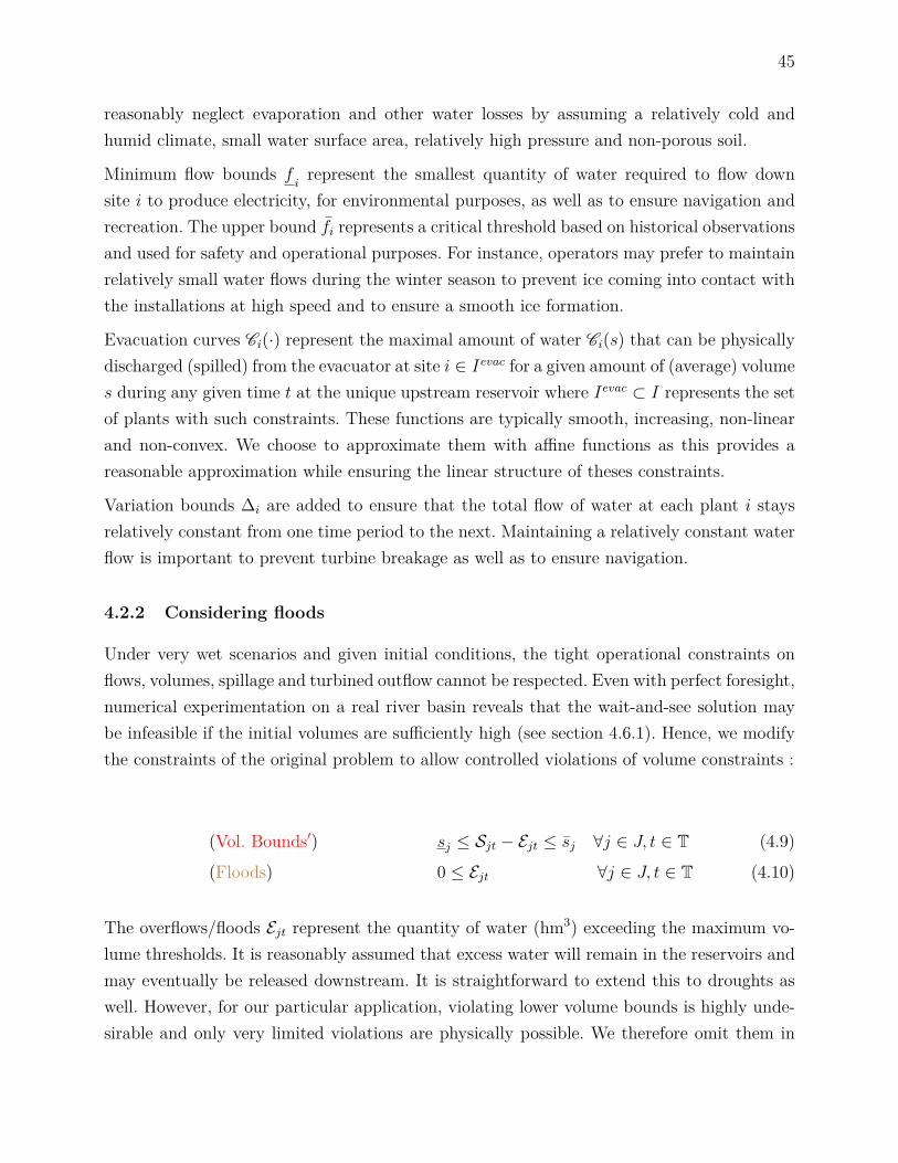
45

reasonably neglect evaporation and other water losses by assuming a relatively cold andhumid climate, small water surface area, relatively high pressure and non-porous soil.

Minimum flow bounds firepresent the smallest quantity of water required to flow down

site i to produce electricity, for environmental purposes, as well as to ensure navigation andrecreation. The upper bound fi represents a critical threshold based on historical observationsand used for safety and operational purposes. For instance, operators may prefer to maintainrelatively small water flows during the winter season to prevent ice coming into contact withthe installations at high speed and to ensure a smooth ice formation.

Evacuation curves Ci(·) represent the maximal amount of water Ci(s) that can be physicallydischarged (spilled) from the evacuator at site i ∈ Ievac for a given amount of (average) volumes during any given time t at the unique upstream reservoir where Ievac ⊂ I represents the setof plants with such constraints. These functions are typically smooth, increasing, non-linearand non-convex. We choose to approximate them with affine functions as this provides areasonable approximation while ensuring the linear structure of theses constraints.

Variation bounds ∆i are added to ensure that the total flow of water at each plant i staysrelatively constant from one time period to the next. Maintaining a relatively constant waterflow is important to prevent turbine breakage as well as to ensure navigation.

4.2.2 Considering floods

Under very wet scenarios and given initial conditions, the tight operational constraints onflows, volumes, spillage and turbined outflow cannot be respected. Even with perfect foresight,numerical experimentation on a real river basin reveals that the wait-and-see solution maybe infeasible if the initial volumes are sufficiently high (see section 4.6.1). Hence, we modifythe constraints of the original problem to allow controlled violations of volume constraints :

(Vol. Bounds′) sj ≤ Sjt − Ejt ≤ sj ∀j ∈ J, t ∈ T (4.9)(Floods) 0 ≤ Ejt ∀j ∈ J, t ∈ T (4.10)

The overflows/floods Ejt represent the quantity of water (hm3) exceeding the maximum vo-lume thresholds. It is reasonably assumed that excess water will remain in the reservoirs andmay eventually be released downstream. It is straightforward to extend this to droughts aswell. However, for our particular application, violating lower volume bounds is highly unde-sirable and only very limited violations are physically possible. We therefore omit them in

46

our formulation.

4.2.3 Evaluating floods over the entire horizon for the whole hydro electricalcomplex

We seek a solution that minimizes these floods over all reservoirs and time periods. These ob-jectives may be conflicting as variations in volumes upstream may have important cascadingeffects on downstream reservoirs. This approach is tantamount to numerous hydro electricalcomplexes in the presence of nearby riparian human populations and infrastructure as wellas fauna and flora.

It is also crucial to consider the relative importance of floods as they may have widely varyingconsequences depending on the segments of the river where they occur, the time of the yearand their magnitude. We tackle this problem by considering the positive linear combinationsof floods ∑j∈J

∑Tt=1(κjtEjt) with parameters κjt > 0, ∀j, t and E = (E11, · · · , E|J |T )> ∈ R|J |T .

To reflect the importance of reservoirs located near riparian populations and high risks offloods as well as those with critical importance, we define the set J crit and fix κjt = Wκ, ∀j ∈J crit, t for some largeW ∈ N and κ ∈ R. Since the relative importance of upper volume boundsat each of the reservoirs in J \J crit is similar, we fix κjt = κ, ∀j ∈ J \J crit, t. For our specificapplication, this categorization is clearly defined, but identifying the relative importance ofviolations may require using preference assessment tools such as MACBETH (Bana e Costaand Vansnick, 1997). We choose κ such that the sum of weights is equal to 1 and keep itconstant with respect to time since we consider a small time horizon.

Although we use the simple linear penalization term κjtEjt for fixed j and t, it would bestraightforward to consider convex piecewise linear functions. It would also be possible touse other convex functions such as convex quadratic functions and then obtain conservativepolyhedral approximations as we do in Section 4.6.1 for the evacuation curves. Consideringmore general non-convex functions such as the ones used in Pianosi and Soncini-Sessa (2009)could perhaps be done through non-convex piecewise linear functions, but would requireusing a mixed-integer program, which would significantly increase the computational requi-rements compared to our proposed approach and reduce its practical applicability for rivermanagement. After discussions with Hydro-Québec, the simple linear penalization functionwas deemed appropriate for our needs.

47

4.3 Incorporating inflow uncertainty

In most river systems, there is a considerable amount of uncertainty surrounding inflows. Thisrandomness is one of the main driving forces in the variability of the state of the system.For these reasons, we let (Ω,F , Ft,P) be a filtered probability space where ξt : Ω →R, ∀t ∈ 1, · · · , T represents the total inflows (in m3/s) for the river basin at time t, F isa σ-algebra and Ft is the natural filtration induced by the stochastic process ξtt=1,··· ,T

where Ft = σ(ξs, s < t) ⊂ F = FT . The random vector ξ[t] = (ξ1, · · · , ξt)> represents thepast inflows up time t and ξ ≡ ξ[T ].

We denote E the expectation operator and assume that E[ξt] = µt <∞ and E[(ξt−µt)2] 12 =

σt < ∞ for all t. These moments are estimated with their corresponding non-parametricsample statistics. For the random variable ξt : Ω → R, we denote ess sup ξt = infa ∈R : P(ξt > a) = 0. We assume ζt = ξt − µt is essentially bounded and that the compactand convex set Zν ⊂ RT represents the true support of the probability measure Pζ = P ζ−1 with fixed parameter 0 ≤ ν < ∞. More precisely, we assume Zν = ζ ∈ RT : ζt ∈[−minνσt, µt, νσt], ∀t since ξt = ζt + µt ≥ 0 with Pζ a.s. ∀t.

We choose this uncertainty set because of its simplicity and numerical efficiency. It also allowsus to obtain simple probabilistic bounds on individual random variables. Indeed, for any fixedt, Tchebyshev’s inequality yields P (ζt ∈ [−minνσt, µt, νσt]) = P (|ζt| ≤ νσt) ≥ 1 − ν−2.In any case, this can be considered a basic assumption of our model. Nonetheless, we testedthe performance of our method with the budgeted uncertainty and present some results inSections 4.6.3 and 4.6.6.

We assume a relatively small river basin where inflows at each reservoir are perfectly correla-ted. Although our method can easily consider the case of independent or partially spatiallycorrelated inflows, this would increase the computational burden and complicate the exposi-tion of the problem. In the case of perfectly spatially correlated inflows, we can represent ξjt,the total water inflow in m3/s from natural precipitations and spring thaw going in reservoirj at time t as ξjt(ζ) = µjt + ζtαjt where αjt = µjt(

∑j µjt)−1 is the expected proportion of the

total inflows entering the reservoir at that time.

4.4 Risk analysis

4.4.1 Conditional value-at-risk

To evaluate the riskiness of floods over all reservoirs and time periods, we evaluate theconditional value at risk of the total weighted floods over the entire horizon for the hydro-

48

electrical complex that was presented earlier in Section 4.2.3 for a fixed α ∈ [0, 1] :

CVaRα(∑j∈J

T∑t=1

(κjtEjt)) (4.11)

The conditional value at risk is a coherent risk measure (Artzner et al., 1999; Rockafellarand Uryasev, 2002; Acerbi and Tasche, 2002). If U is a continuous random variable boundedwith probability 1, then CVaRα(U) = E[U|U > VaRα(U)] holds for α ∈ (0, 1). In otherwords, CVaRα(U) represents the conditional expectation of U given that it is greater thanthe (1 − α) left quantile VaRα(U) = infu ∈ R : P(U ≤ u) ≥ 1 − α for a given α ∈ (0, 1).We can thus interpret the risk of U , as the average of the worst α100% of values for someα ∈ (0, 1)(see Acerbi and Tasche (2002)). As observed in financial applications, CVaRα offersthe important property of considering all the realizations of a random variable in the "worst"α-tail of the distribution. As α→ 1, we consider more realizations, but reduce the weight ofextremely bad realizations. For a continuous random variable U , we also have :

limα→1

CVaRα(U) = E[U ] and limα→0

CVaRα(U) = ess supU (4.12)

that correspond to the natural risk neutral approach and to the totally risk averse approachused in robust optimization. Both E and ess sup also correspond to coherent risk measures.Furthermore, we have the relationship E[U ] ≤ CVaRα(U) ≤ ess supU , ∀α ∈ (0, 1).

The conditional value-at-risk can also be written as the following optimization problem :CVaRα(U) = inft∈Rt + α−1E[maxU − t, 0]. CVaRα therefore represents a very naturaland flexible risk measure and offers the possibility to explore the impact of various risktolerance and model conservativeness through sensitivity analysis on the α parameter.

Recent studies based on coherent risk measures and other statistical functionals have shownthe value of incorporating risk aversion into the decision process (Shapiro et al., 2013; Babaeiet al., 2015; Artus et al., 2006). Like some of these works, we highlight the fact that riskaversion can be introduced at little or no computational cost compared with the traditionalrisk neutrality.

49

4.4.2 Dynamic risk measures and time consistency

Our optimization model evaluates the risk measure CVaRα at the beginning of the entirehorizon once in a static fashion. For α ∈ (0, 1), this approach may lead to solutions thatviolate the concept of time-consistency. This notion is related to Bellman’s principle and canloosely be interpreted as the requirement that optimal decisions taken at a given time fora fixed horizon should remain optimal when the problem is solved again at any other laterdate (see Acciacio and Penner (2011) for more details on dynamic risk measures). Althoughthis issue is important in a dynamic decision making environment, we omit to address it inour model because there has been little work on tractable representations of time-consistentstochastic problems using dynamic risk measures except in simple cases such as seriallyindependent random variables when considering the risk neutral expectation (see Shapiro(2009)).

4.5 Stochastic model and choice of decision rules

We consider a dynamic setting were the true realization of the random process is pro-gressively revealed as time unfolds over the horizon of T days. A sequence of controlsX1, · · · ,Xt must be fixed at each stage t = 1, · · · , T after observing the realized historyζ[t−1](ω) = (ζ1, · · · , ζt−1)>(ω), but before knowing the future values (ζt, · · · , ζT )>(ω). At eachtime t = 1, · · · , T , we optimize over the class of bounded functions of the form Xt : RT → Rnt ,∑T−1t=0 nt = n. Hence, we convert the decision variables of our deterministic model 3into more

flexible functions.

Real implementable decisions must be non-anticipative such that Xt ζ must be Ft−1 mea-surable. Once ζ[t−1](ω) is known, they can be implemented to yield the actual decisionsXt(ζ[t−1](ω)) ∈ Rnt . We may interchangeably refer to X as controls or decision rules anduse the notation X = (X>1 , · · · ,X>T )>. The aggregate decision rule Xt = (S>t ,L>t , R>t ,F>t ,E>t )> is simply the stacking of each decision at time t. Refer to Table 4.1 for identification ofimplementable decisions.

4.5.1 Affine decision rules

In order to obtain an upper bound on the optimal value of our stochastic programmingproblem, we first consider decision rules that are affine in ζ. If Kt = nt−1 +1, · · · , nt−1 +ntrepresents the indices associated with decisions at time t ≥ 1 and n0 = 0, we can write thecontrols in the form :

3. We can see the decision variables of our deterministic model as constant functions of the uncertainty.

50

Xkt(ζ) = X 0kt +

T∑t′=1X t′

ktζt′ , k ∈ Kt (4.13)

where X 0kt,X t′

kt ∈ R, ∀k ∈ Kt, t′ ∈ 1, · · · , T. In order to ensure that controls that represent

real implementable decisions are non-anticipative, it is sufficient to force X t′kt = 0, ∀k ∈

K It , t = 1, · · · , T, t′ ≥ t where K I

t ⊂ Kt represents the set of indices associated with realimplementable decisions.

The volumes, droughts and floods can also be anticipative, since they represent analy-sis/auxiliary variables that are only required for computation (refer to Table 4.1). Because ofthe full-dimensionality of Zν and the additive uncertainty, flow conservation constraints (4.2)are satisfied by solving a non-homogeneous linear system of equations in X t′

kt,X 0kt (see Lorca

et al. (2016) for example and Section 4.9.3 of the Appendix for a detailed formulation).

We reformulate the variation of flow constraints across time by writing :

(Fit −Fit−1)(ζ) ≤ ∆i, ∀i, t = 2, · · · , T (4.14)−(Fit −Fit−1)(ζ) ≤ ∆i, ∀i, t = 2, · · · , T (4.15)

where all constraints must hold ∀ζ ∈ Zν . As mentioned previously, we consider affine ap-proximations of the real maximum spillage constraints : Ci : v → C 0

i +C ∆i v with C 0

i ,C∆i ∈ R

for all plants i ∈ Ievac. Hence if j−(i) indicates the unique reservoir upstream of plant i, thefollowing evacuation curve constraints must hold ∀ζ ∈ Zν :

Lit(ζ) ≤ C 0i + C ∆

i Sj−(i)t(ζ), ∀i ∈ Ievac, t (4.16)

4.5.2 Objective function formulation for robust problem

To express our objective function, we exploit the formulation of CVaRα as an optimiza-tion problem. Indeed, for α ∈ (0, 1) and random variable X ∈ L∞, we have CVaRα(X) =inft∈Rt+ 1

αE[maxX − t, 0]. This corresponds to the definition of Pflug (2000), where we

have replaced 1− α by α so that the CVaRα we consider is non-increasing in α.

To obtain a conservative (upper bound) on CVaRα(∑j∈J∑Tt=1(κjtE+

jt(ζ))), we consider theanticipative decision rule D(ζ) = D0 + ∑T

t′=1Dt′ζt′ where E[D(ζ)] = D0 since we consider

51

affine decision rules and E[ζt] = 0,∀t without loss of generality. We then add the decisionvariables ϕ, t ∈ R as well as the following constraints :

t+ 1αD0 ≤ ϕ (4.17)

D(ζ) ≥ 0 (4.18)

D(ζ) ≥∑j∈J

T∑t=1

(κjtEjt(ζ))− t (4.19)

that must hold ∀ζ ∈ Zν . We finally set ϕ as the objective function to minimize. Constraints(4.18)-(4.19) model D(ζ) ≥ max∑j∈J

∑Tt=1(κjtEjt(ζ))− t, 0, ∀ζ ∈ Zν .

The case α = 0 is handled separately by adding the variable ϕ and the constraintϕ ≥ ∑

j∈J∑Tt=1(κjtEjt(ζ)),∀ζ ∈ Zν . Hence minimizing ϕ yields ess sup(∑j

∑Tt=1 Ejt(ζ)κjt) =

maxζ∈Zν∑j∈J

∑Tt=1(κjtEjt(ζ)), which is the worst case if we only consider support information

and corresponds to the classical robust objective.

The case α = 1 (expected value) is treated by adding ϕ and ϕ ≥ ∑j∈J

∑Tt=1(κjtE0+

jt ) =E[∑j

∑Tt=1 Ejt(ζ)κjt]. In all cases, we use this epigraph form and set ϕ as the objective value

to minimize. Since we restrict ourselves to a limited class of decision rules, it follows that theoptimal solution of our problem (given by ϕ∗) bounds the true risk from above.

The rest of the constraints are readily obtained from the deterministic problem where wereplace decision variables with their associated affine decision rules. Deriving the deterministicequivalent program is straightforward by using well known methods from robust optimization.For all the inequality constraints that are meant to hold ∀ζ ∈ Zν , we namely use strong linearprogramming duality, which is possible since Zν is a non-empty compact polyhedron. Therobust equivalent is explicitly computed for a representative inequality in Section 4.9.1 of theAppendix.

4.5.3 Affine decision rules on lifted probability space

In order to obtain a better upper bound on the optimal solution of our risk averse stochasticprogram, we consider a special case of the lifted decision rules of Georghiou et al. (2015).Since we follow their work closely, we give a brief treatment of these decisions rules. However,we provide a detailed discussion with an example in the Appendix to help build the intuitionof the reader.

The general idea is to apply a non-linear transformation L′ : RT → RrT for some r ∈ N to Zν

52

in order to lift the random vector ζ ∈ RT onto a higher dimensional space : L′(ζ) = ζ ′′ ∈ RrT .Under our choice of L′, which we describe shortly, the set L′(Zν) is non-convex. It thereforebecomes convenient to consider an exterior convex approximation Z ′′ν ⊃ L′(Zν). We thendefine the retraction operator R′ : RrT → RT such that (R′ L′) = I and impose thatR′ζ ′′ ∈ Zν for all points ζ ′′ ∈ Z ′′ν .

By considering controls that are affine functions of the new lifted random variables ζ ′′ ∈ RrT ,the decisions rules (4.13) become :

Xkt(ζ ′′) = X 0kt +

T∑t′=1

r∑s=1X t′skt ζ

′′t′,s k ∈ Kt (4.20)

and we can express the robust counterpart directly in terms of ζ ′′. By restricting the coeffi-cients of our new lifted affine decision rules (4.20), we can always obtain the initial (unlifted)affine decision rules. Hence, with this choice of Z ′′ν , L′ and R′, the lifted problem provides anupper bound that is at least as good as the one with the original affine decisions.

The heart of the problem is then to judiciously define L′ and the corresponding R′ in order tomaintain the tractability of the new lifted program while ensuring an efficient representationof the feasible domain of the lifted random variables and improving the upper bound onthe optimal solution of our program. We fix L

′ = L F where L is a non-linear bijectivemapping and F : RT → RT is a simple bijective linear mapping (F−1 is a T × T matrix thatexists) preserving the non-anticipativity of decision rules (Fij = 0, ∀i < j) and that can beinterpreted as a change of basis. It is possible to consider non-invertible mappings, but weignore this case for sake of simplicity (see Georghiou et al. (2015)).

The non-linear operator L : RT → RrT is defined through the partial lifting Lt : R → Rr asfollows :

Ltk(ζ′) =

minζ ′t , zt1 if k = 1

max0,minζ ′t , ztk − ztk−1 if k = 2, · · · , r − 1

maxζ ′t − ztk−1, 0 if k = r

for all t where zt1 < zt2 < · · · < ztr−1 are breakpoints dividing the range of the original ζ ′t in rdimensions. Similarly, we define the partial (linear) retraction operator Rt : Rr → R, ∀t asfollows :

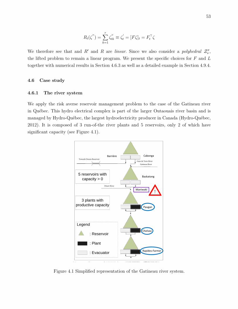
53

Rt(ζ′′) =

r∑k=1

ζ′′

tk ≡ ζ′

t = [Fζ]t = F>t ζ

We therefore see that and R′ and R are linear. Since we also consider a polyhedral Z ′′ν ,the lifted problem to remain a linear program. We present the specific choices for F and Ltogether with numerical results in Section 4.6.3 as well as a detailed example in Section 4.9.4.

4.6 Case study

4.6.1 The river system

We apply the risk averse reservoir management problem to the case of the Gatineau riverin Québec. This hydro electrical complex is part of the larger Outaouais river basin and ismanaged by Hydro-Québec, the largest hydroelectricity producer in Canada (Hydro-Québec,2012). It is composed of 3 run-of-the river plants and 5 reservoirs, only 2 of which havesignificant capacity (see Figure 4.1).

5 reservoirs with

capacity > 0

3 plants with

productive capacity

CabongaBarrière

Baskatong

Maniwaki

Paugan

Chelsea

Legend

: Reservoir

: Plant

: Evacuator

!

Towards Dozois Reservoir

Gatineau RiverGens e erre River

Désert River

Rapides-Farmer

Figure 4.1 Simplified representation of the Gatineau river system.

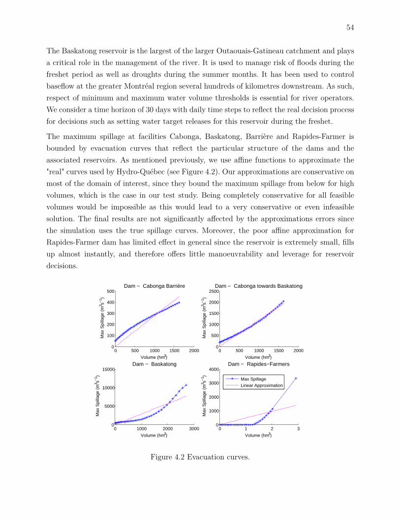
54

The Baskatong reservoir is the largest of the larger Outaouais-Gatineau catchment and playsa critical role in the management of the river. It is used to manage risk of floods during thefreshet period as well as droughts during the summer months. It has been used to controlbaseflow at the greater Montréal region several hundreds of kilometres downstream. As such,respect of minimum and maximum water volume thresholds is essential for river operators.We consider a time horizon of 30 days with daily time steps to reflect the real decision processfor decisions such as setting water target releases for this reservoir during the freshet.

The maximum spillage at facilities Cabonga, Baskatong, Barrière and Rapides-Farmer isbounded by evacuation curves that reflect the particular structure of the dams and theassociated reservoirs. As mentioned previously, we use affine functions to approximate the"real" curves used by Hydro-Québec (see Figure 4.2). Our approximations are conservative onmost of the domain of interest, since they bound the maximum spillage from below for highvolumes, which is the case in our test study. Being completely conservative for all feasiblevolumes would be impossible as this would lead to a very conservative or even infeasiblesolution. The final results are not significantly affected by the approximations errors sincethe simulation uses the true spillage curves. Moreover, the poor affine approximation forRapides-Farmer dam has limited effect in general since the reservoir is extremely small, fillsup almost instantly, and therefore offers little manoeuvrability and leverage for reservoirdecisions.

0 500 1000 1500 20000

100

200

300

400

500Dam − Cabonga Barrière

Volume (hm3)

Max

Spi

llage

(m

3 s−1 )

0 500 1000 1500 20000

500

1000

1500

2000

2500Dam − Cabonga towards Baskatong

Volume (hm3)

Max

Spi

llage

(m

3 s−1 )

0 1000 2000 30000

5000

10000

15000Dam − Baskatong

Volume (hm3)

Max

Spi

llage

(m

3 s−1 )

0 1 2 30

1000

2000

3000

4000

Volume (hm3)

Max

Spi

llage

(m

3 s−1 )

Dam − Rapides−Farmers

Max SpillageLinear Approximation

Student Version of MATLAB

Figure 4.2 Evacuation curves.

55

Although there are no structures to control water outflow near Maniwaki, there are extremelytight constraints on maximum and minimum flow at that river segment. These bounds re-present critical outflow level used to control the risk of drought and flood for the neighbouringtown and are therefore essential.

The Gatineau represents an excellent case study as it has relatively small productive capacitycompared to the rest of the park. More importantly, the river runs near the small town ofManiwaki that is subject to high risks of flooding, particularly during the spring freshet.Indeed, the city has suffered 4 significant floods in 1929, 1936, 1947 and 1974.

Even today, there exists a need to mitigate the risk of these natural disasters. As Figure4.3 illustrates, it is possible that we fail to find a solution eliminating all floods even whenwe have perfect foresight. This is namely the case when ζt = µt + 2σt, ∀t. Although thissynthetic scenario is wet over the entire month, it remains plausible because of the strongserial correlation of inflows as well as evidence from past observations. In this case, even ifwe spill as much as possible at Baskatong so that the total flow at Maniwaki downstream isconstantly at its upper bound, the deterministic program cannot prevent the reservoir fromfilling up and eventually flooding.

0 5 10 15 20 25 300

500

1000

1500

2000

2500

3000

3500

Time

hm3

Synthetic scenario: µt+2σt, ∀ t

Floods

Student Version of MATLAB

Figure 4.3 Violations with perfect foresight.

4.6.2 The inflows

Based on our sample observations, the assumption of perfectly spatially correlated inflows isnot unreasonable for the Gatineau river. As is clear from the Figure 4.4, water inflows areparticularly important during the months of March through April (freshet) as snow melts.There is a second surge during fall caused by greater precipitations and finally there are very

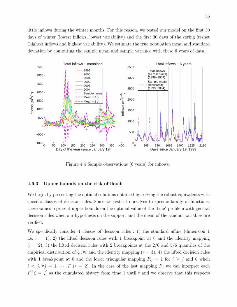
56

little inflows during the winter months. For this reason, we tested our model on the first 30days of winter (lowest inflows, lowest variability) and the first 30 days of the spring freshet(highest inflows and highest variability). We estimate the true population mean and standarddeviation by computing the sample mean and sample variance with these 6 years of data.

0 50 100 150 200 250 300 350 400−1000

−500

0

500

1000

1500

2000

2500

3000

3500

Day of the year (since January 1st)

Total inflows − combined

199920002001200220032004Sample meanMean + 2 σMean − 2 σ

0 365 730 1095 1460 1825 21900

500

1000

1500

2000

2500

3000

3500

Days since January 1st 1999

Inflo

ws

(m3 s−

1 )

Total inflows − 6 years

Total inflows(all reservoirs)(1999−2004)Sample mean(replicated)(1999−2004)

Student Version of MATLAB

Inflo

ws

(m3 s−

1 )

Figure 4.4 Sample observations (6 years) for inflows.

4.6.3 Upper bounds on the risk of floods

We begin by presenting the optimal solutions obtained by solving the robust equivalents withspecific classes of decision rules. Since we restrict ourselves to specific family of functions,these values represent upper bounds on the optimal value of the "true" problem with generaldecision rules when our hypothesis on the support and the mean of the random variables areverified.

We specifically consider 4 classes of decision rules : 1) the standard affine (dimension 1i.e. r = 1), 2) the lifted decision rules with 1 breakpoint at 0 and the identity mapping(r = 2), 3) the lifted decision rules with 2 breakpoints at the 2/6 and 5/6 quantiles of theempirical distribution of ζt,∀t and the identity mapping (r = 3), 4) the lifted decision ruleswith 1 breakpoint at 0 and the lower triangular mapping Fij = 1 for i ≥ j and 0 wheni < j, ∀j = 1, · · · , T (r = 2). In the case of the last mapping F , we can interpret eachF>t ζ = ζ

′t as the cumulated history from time 1 until t and we observe that this respects

57

non-anticipativity. We attempted to solve the model with the same mapping F and r = 3,but ran into computational difficulties since the problem could not be solved in less than 3days. As we discuss later in this Section, this is likely a consequence of the high degeneracyof the linear program.

All solutions where obtained by setting ν = 3, which ensured the support contained allhistorical inflows from 1999-2004 and provided good quality solutions across all models. Wetested our models with varying values of ν and found that increasing its value above a certainthreshold leads to infeasibility issues as all bounds cannot be simultaneously respected forvery large uncertainty sets. As expected, small ν’s lead the model to predict small violations.However, the solutions displayed poor performance when tested on realistic inflows that didnot belong to the uncertainty set. Our sensitivity analysis did not seem to reveal any clearlink between the size of ν and the performance of our models when tested with ζ 6∈ Zν .

The upper bounds are displayed in the line "Optimal solution" of Table 4.2. These values aregood indicators of the CVaR of volume violations at Baskatong predicted by the model. Itis therefore interesting to compare them with the empirical CVaR of violations presented inFigure 4.7 of Section 4.6.6.

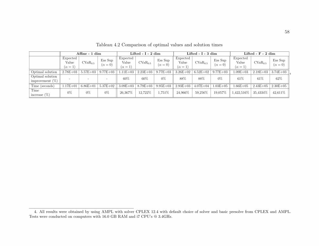
58

Tableau 4.2 Comparison of optimal values and solution times

Affine - 1 dim Lifted - I - 2 dim Lifted - I - 3 dim Lifted - F - 2 dimExpectedValue(α = 1)

CVaR0.5Ess Sup(α = 0)

ExpectedValue(α = 1)

CVaR0.5Ess Sup(α = 0)

ExpectedValue(α = 1)

CVaR0.5Ess Sup(α = 0)

ExpectedValue(α = 1)

CVaR0.5Ess Sup(α = 0)

Optimal solution 2.78E+03 5.57E+03 9.77E+03 1.11E+03 2.23E+03 9.77E+03 3.26E+02 6.52E+02 9.77E+03 1.09E+03 2.18E+03 3.74E+03Optimal solutionimprovement (%) - - - 60% 60% 0% 88% 88% 0% 61% 61% 62%

Time (seconds) 1.17E+01 6.86E+01 5.37E+02 3.09E+03 8.79E+03 9.95E+03 2.93E+03 4.07E+04 1.03E+05 1.66E+05 2.43E+05 2.30E+05Timeincrease (%) 0% 0% 0% 26,367% 12,722% 1,751% 24,966% 59,256% 19,057% 1,422,516% 35,4334% 42,611%

4

4. All results were obtained by using AMPL with solver CPLEX 12.4 with default choice of solver and basic presolve from CPLEX and AMPL.Tests were conducted on computers with 16.0 GB RAM and i7 CPU’s @ 3.4GHz.

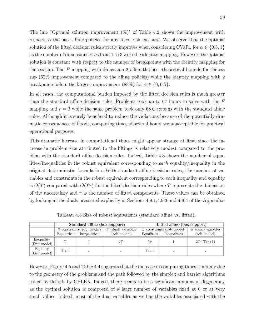
59

The line "Optimal solution improvement (%)" of Table 4.2 shows the improvement withrespect to the base affine policies for any fixed risk measure. We observe that the optimalsolution of the lifted decision rules strictly improves when considering CVaRα for α ∈ 0.5, 1as the number of dimensions rises from 1 to 3 with the identity mapping. However, the optimalsolution is constant with respect to the number of breakpoints with the identity mapping forthe ess sup. The F mapping with dimension 2 offers the best theoretical bounds for the esssup (62% improvement compared to the affine policies) while the identity mapping with 2breakpoints offers the largest improvement (88%) for α ∈ 0, 0.5.

In all cases, the computational burden imposed by the lifted decision rules is much greaterthan the standard affine decision rules. Problems took up to 67 hours to solve with the Fmapping and r = 2 while the same problem took only 68.6 seconds with the standard affinerules. Although it is surely beneficial to reduce the violations because of the potentially dra-matic consequences of floods, computing times of several hours are unacceptable for practicaloperational purposes.

This dramatic increase in computational times might appear strange at first, since the in-crease in problem size attributed to the liftings is relatively modest compared to the pro-blem with the standard affine decision rules. Indeed, Table 4.3 shows the number of equa-lities/inequalities in the robust equivalent corresponding to each equality/inequality in theoriginal deterministic formulation. With standard affine decision rules, the number of va-riables and constraints in the robust equivalent corresponding to each inequality and equalityis O(T ) compared with O(Tr) for the lifted decision rules where T represents the dimensionof the uncertainty and r is the number of lifted components. These values can be obtainedby looking at the duals presented explicitly in Sections 4.9.1,4.9.3 and 4.9.4 of the Appendix.

Tableau 4.3 Size of robust equivalents (standard affine vs. lifted).

Standard affine (box support) Lifted affine (box support)# constraints (rob. model) # (dual) variables

(rob. model)# constraints (rob. model) # (dual) variables

(rob. model)Equalities Inequalities Equalities InequalitiesInequality

(Det. model) T 1 2T Tr 1 2T+T(r+1)

Equality(Det. model) T+1 - - Tr+1 - -

However, Figure 4.5 and Table 4.4 suggests that the increase in computing times is mainly dueto the geometry of the problems and the path followed by the simplex and barrier algorithmscalled by default by CPLEX. Indeed, there seems to be a significant amount of degeneracyas the optimal solution is composed of a large number of variables fixed at 0 or at verysmall values. Indeed, most of the dual variables as well as the variables associated with the

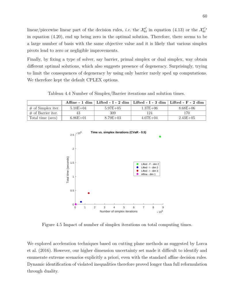
60

linear/piecewise linear part of the decision rules, i.e. the X t′kt in equation (4.13) or the X t′s

kt

in equation (4.20), end up being zero in the optimal solution. Therefore, there seems to bea large number of basis with the same objective value and it is likely that various simplexpivots lead to zero or negligible improvements.

Finally, by fixing a type of solver, say barrier, primal simplex or dual simplex, way obtaindifferent optimal solutions, which also suggests presence of degeneracy. Surprisingly, tryingto limit the consequences of degeneracy by using only barrier rarely sped up computations.We therefore kept the default CPLEX options.

Tableau 4.4 Number of Simplex/Barrier iterations and solution times.

Affine - 1 dim Lifted - I - 2 dim Lifted - I - 3 dim Lifted - F - 2 dim# of Simplex iter. 5.10E+04 5.97E+05 1.37E+06 8.68E+06# of Barrier iter. 43 309 124 170Total time (secs) 6.86E+01 8.79E+03 4.07E+04 2.43E+05

0 1 2 3 4 5 6 7 8 9

Number of simplex iterations #106

0

0.5

1

1.5

2

2.5

Tot

al ti

me

(sec

onds

)

#105 Time vs. simplex iterations (CVaR - 0.5)

Lifted - F - dim 2Lifted - I - dim 2Lifted - I - dim 3Affine - dim 1

Figure 4.5 Impact of number of simplex iterations on total computing times.

We explored acceleration techniques based on cutting plane methods as suggested by Lorcaet al. (2016). However, our higher dimension uncertainty set made it difficult to identify andenumerate extreme scenarios explicitly a priori, even with the standard affine decision rules.Dynamic identification of violated inequalities therefore proved longer than full reformulationthrough duality.

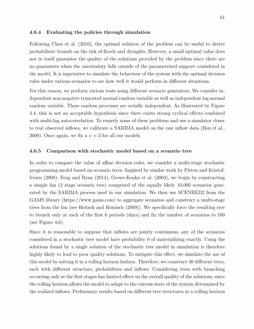
61

4.6.4 Evaluating the policies through simulation

Following Chen et al. (2010), the optimal solution of the problem can be useful to deriveprobabilistic bounds on the risk of floods and droughts. However, a small optimal value doesnot in itself guarantee the quality of the solutions provided by the problem since there areno guarantees when the uncertainty falls outside of the parametrized support considered inthe model. It is imperative to simulate the behaviour of the system with the optimal decisionrules under various scenarios to see how well it would perform in different situations.

For this reason, we perform various tests using different scenario generators. We consider in-dependent non-negative truncated normal random variable as well as independent log normalrandom variable. These random processes are serially independent. As illustrated by Figure4.4, this is not an acceptable hypothesis since there exists strong cyclical effects combinedwith multi-lag autocorrelation. To remedy some of these problems and use a simulator closerto real observed inflows, we calibrate a SARIMA model on the raw inflow data (Box et al.,2008). Once again, we fix a ν = 3 for all our models.

4.6.5 Comparison with stochastic model based on a scenario tree

In order to compare the value of affine decision rules, we consider a multi-stage stochasticprogramming model based on scenario trees. Inspired by similar work by Fleten and Kristof-fersen (2008); Feng and Ryan (2014); Growe-Kuska et al. (2003), we begin by constructinga simple fan (2 stage scenario tree) comprised of the equally likely 10,000 scenarios gene-rated by the SARIMA process used in our simulation. We then use SCENRED2 from theGAMS library (https://www.gams.com) to aggregate scenarios and construct a multi-stagetrees from the fan (see Heitsch and Römisch (2009)). We specifically force the resulting treeto branch only at each of the first 6 periods (days) and fix the number of scenarios to 100(see Figure 4.6).

Since it is reasonable to suppose that inflows are jointly continuous, any of the scenariosconsidered in a stochastic tree model have probability 0 of materializing exactly. Using thesolutions found by a single solution of the stochastic tree model in simulation is thereforehighly likely to lead to poor quality solutions. To mitigate this effect, we simulate the use ofthis model by solving it in a rolling horizon fashion. Therefore, we construct 30 different trees,each with different structure, probabilities and inflows. Considering trees with branchingoccurring only at the first stages has limited effect on the overall quality of the solutions, sincethe rolling horizon allows the model to adapt to the current state of the system determined bythe realized inflows. Preliminary results based on different tree structures in a rolling horizon

62

framework suggests that branching at the early stages is a more important performance driverthan the total number of scenarios considered.

Figure 4.6 Sample multistage tree generated by SCENRED2 from scenario fan.

We also tested affine decision rules in a rolling horizon, but with a shorter lookahead period,namely 1 week. These problems took on average 5 seconds to solve. In comparison, eachproblem based on scenario trees took almost 4 times more time to solve. Because of thesetime limitations, we were only able to simulate the behaviour of the scenario tree with rollinghorizon based on 1,000 random scenarios, rather than the full 10,000. This also explains whywe limited the size and structure of the tree.

4.6.6 Simulation results

We report the empirical conditional value at risk of violations for the three most importantconstraints in Figure 4.7. We namely consider volume violations at Baskatong and Cabonga,the two large reservoirs, as well as the flow violations at the town of Maniwaki, which is acritical flood indicator. We compute the CVaR at different levels of risk α′ = 100(1−α) withα ∈ 0.01, · · · , 0.99. We also show the expected value at α′ = 0 and the ess sup at α′ = 100.All results are obtained by considering 10,000 scenarios, except for the scenario tree, whichconsiders only 1,000, since using a rolling horizon heuristic over the 30-day horizon for 10,000scenarios would take on average more than 40 days.

63

In all cases, we find that the theoretical upper bound found by solving the stochastic modelis loose. Even if we do not restrict the random variables to lie within the support consideredby our model, we find that the empirical CVaRα is usually smaller than the theoretical upperbound.

For sake of space, we present only results for the independent log-normally distributed randomvariables with mean equal to µt and variance set to ν ′σt at every t = 1, · · · , T for a givenν ′ ∈ R+

5. The µt and σt are the same values as the ones considered in the uncertainty sets.Although we use 1 ≤ ν ′ < ν, we consider the full support of the random variables (0,∞) anddo not restrict the realisations to the box considered by the model. Results for the normalindependent variables and the SARIMA time series are similar in nature, even if the scenariotree is constructed with some knowledge of the inflows’ serial correlation.

Increasing the value of ν ′ from its standard value changes the shape of the empirical dis-tribution, but the relative performance of each model stays relatively constant. Moreover,excessively increasing ν ′ may lead to scenarios that are more extreme than natural and thatmay have limited practical interpretation. The treatment of rare extreme events is an openquestion we do not wish to tackle here.

Figure 4.8 presents the empirical CVaRα of violations for the three reservoirs for a fixedpolicy. These can be seen as parametric curves where the α′ is progressively increased from0 to 100. Thus the curves can be read by starting at the (0, 0, 0) point and moving to theupper (104, 6× 103, 60) point.

As Figure 4.8 illustrates, when considering a fixed policy, different risk measures may lead tosolutions that are empirically dominated by others. For instance with the lifted affine decisionrules, mapping I and 2 dimensions, the solution provided by minimizing CVaRα seems to bedominated by the two others since it lies above the curves. However, the situation is reversedfor the lifted affine decision rules, mapping F and 2 dimensions. In this case, the solutionprovided by minimizing CVaRα seems better than the two others.

In most cases, Figure 4.8 suggests that the policy results are similar for all three risk measures.The policies often have the most noticeable differences in the most extreme scenarios, whichrarely occur. However, for the scenario tree with rolling horizon, the policy performances areconsiderably different, particularly for the violations at Baskatong. This does not seem tobe a consequence of the reduced number of simulations, since most results stabilized aftera relatively limited number of simulations. It is possible that by exploiting the probabilities

5. Here ν′ is a parameter controlling the variability of the simulated random variables. We always perfor-med simulations with 1 ≤ ν′ to test the robustness of our solutions.

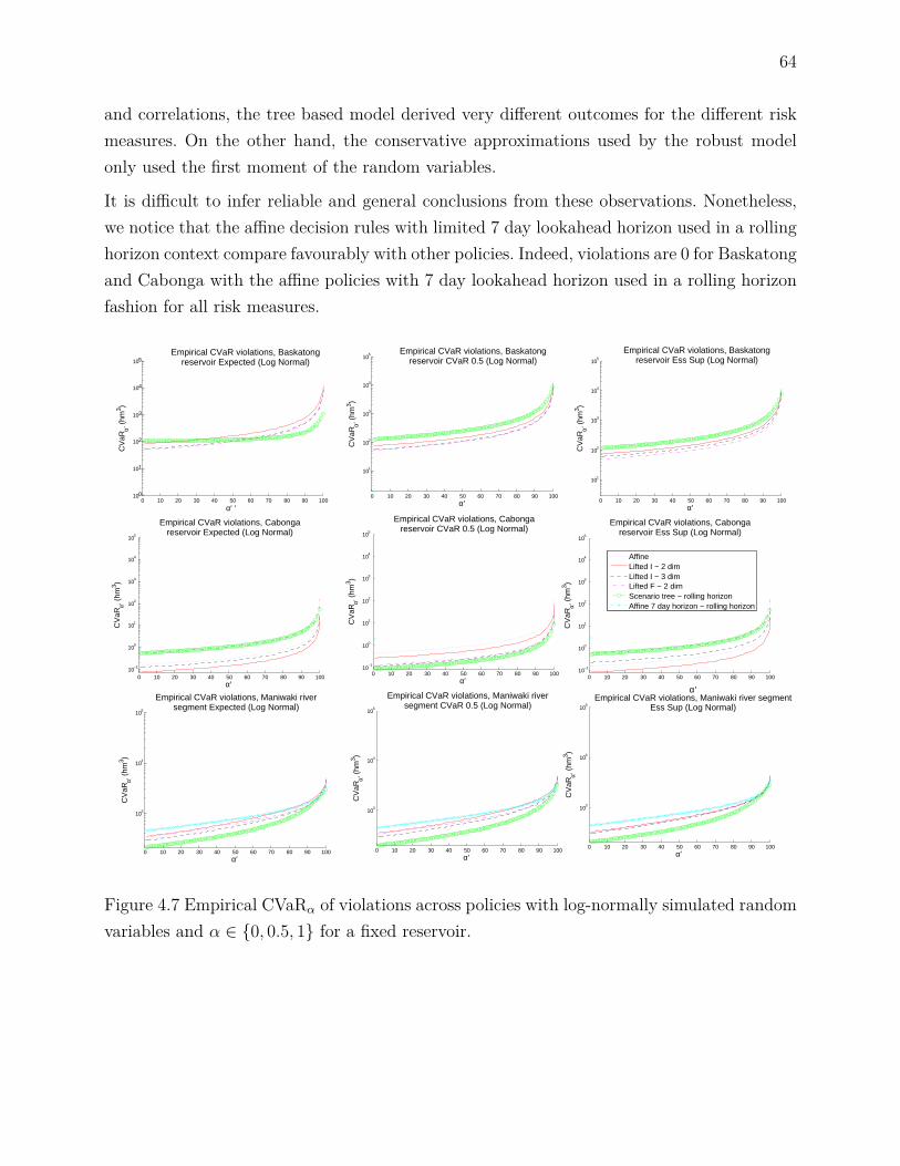
64

and correlations, the tree based model derived very different outcomes for the different riskmeasures. On the other hand, the conservative approximations used by the robust modelonly used the first moment of the random variables.

It is difficult to infer reliable and general conclusions from these observations. Nonetheless,we notice that the affine decision rules with limited 7 day lookahead horizon used in a rollinghorizon context compare favourably with other policies. Indeed, violations are 0 for Baskatongand Cabonga with the affine policies with 7 day lookahead horizon used in a rolling horizonfashion for all risk measures.

0 10 20 30 40 50 60 70 80 90 100100

101

102

103

104

105Empirical CVaR violations, Baskatong

reservoir Expected (Log Normal)

α′ ′

CV

aRα′

(hm

3 )

0 10 20 30 40 50 60 70 80 90 100

101

102

103

104

105 Empirical CVaR violations, Baskatong

reservoir CVaR 0.5 (Log Normal)

α′

CV

aRα′

(hm

3 )

0 10 20 30 40 50 60 70 80 90 100

101

102

103

104

105

Empirical CVaR violations, Baskatong reservoir Ess Sup (Log Normal)

α′

CV

aRα′

(hm

3 )

0 10 20 30 40 50 60 70 80 90 10010

−1

100

101

102

103

104

105

Empirical CVaR violations, Cabonga reservoir Expected (Log Normal)

α′

CV

aRα′

(hm

3 )

0 10 20 30 40 50 60 70 80 90 10010

−1

100

101

102

103

104

105

Empirical CVaR violations, Cabonga reservoir CVaR 0.5 (Log Normal)

α′

CV

aRα′

(hm

3 )

0 10 20 30 40 50 60 70 80 90 10010

−1

100

101

102

103

104

105

Empirical CVaR violations, Cabonga reservoir Ess Sup (Log Normal)

CV

aRα′

(hm

3 )AffineLifted I − 2 dimLifted I − 3 dimLifted F − 2 dimScenario tree − rolling horizonAffine 7 day horizon − rolling horizon

0 10 20 30 40 50 60 70 80 90 100

103

104

105

Empirical CVaR violations, Maniwaki river segment Expected (Log Normal)

α′

CV

aRα′

(hm

3 )

0 10 20 30 40 50 60 70 80 90 100

103

104

105

Empirical CVaR violations, Maniwaki river segment CVaR 0.5 (Log Normal)

α′

CV

aRα′

(hm

3 )

0 10 20 30 40 50 60 70 80 90 100

103

104

105

α′Empirical CVaR violations, Maniwaki river segment

Ess Sup (Log Normal)

α′

CV

aRα′

(hm

3 )

Figure 4.7 Empirical CVaRα of violations across policies with log-normally simulated randomvariables and α ∈ 0, 0.5, 1 for a fixed reservoir.

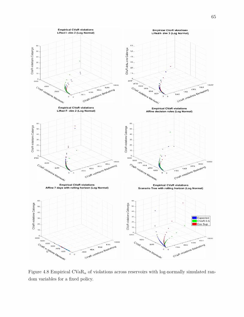
65

"' 0) C:

"'

u "' C:

0

·;:;

Cl'.'. "'

u

60

50

40

30

20

10

6000

C 4000

Ii' 00

Empirical CVaR violations

Lifted I- dim 2 (Log Normal)

. .

:::

vt· 'o,., 0 :s-%

,., . :tii-f,.

10000

"' 0) C:

"'

u "' C:

0

·;:;

Cl'.'. "'

u

60

50

40

30

20

10

Empirical CVaR violations

Lifted F- dim 2 (Log Normal)

10000

60

"' en

50 C:

0 .0

"'

<.)

VJ C:

0

0 ·;;

Cl'. "'

<.)

40

30

20

10

0

6000

5000

Empirical CVaR violations

Affine decision rules (Log Normal)

. .

10000

8000

Empirical CVaR violations

Affine 7 days with rolling horizon (Log Normal)

60 "' CJ) C 50 0

.0

"'

u

"'

40 C

0

30 0 ·;;:

Cl:'. 20 "'

> u 10

0 6000

5000 10000

C

4000

/i> 3000

0ai>oa,., 1000 0 0 u'

I)'·

ti-f;

60

"'

C: 0

(.) (/) C: 0

0

·5

ll'. "'

(.)

40

30

20

10

0

6000

Empirical CVaR violations

Scenario Tree with rolling horizon (Log Normal)

•Expected •cvaR0.5

•EssSup

10000

Figure 4.8 Empirical CVaRα of violations across reservoirs with log-normally simulated ran-dom variables for a fixed policy.

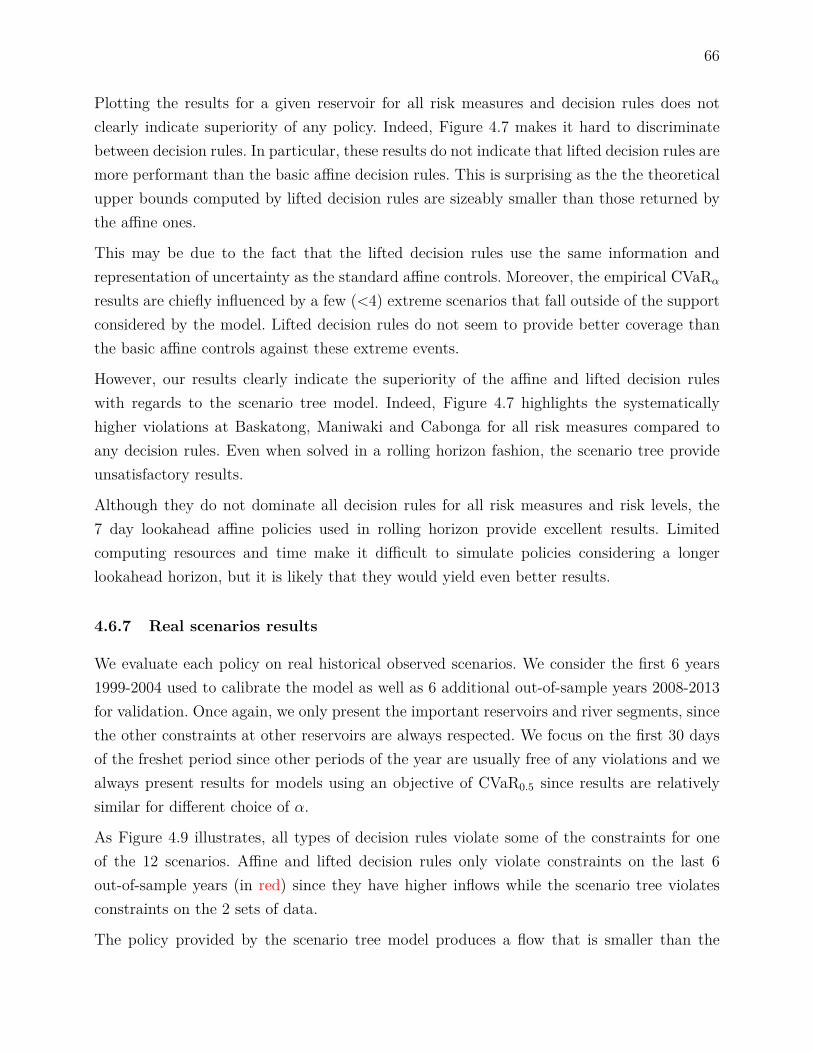
66

Plotting the results for a given reservoir for all risk measures and decision rules does notclearly indicate superiority of any policy. Indeed, Figure 4.7 makes it hard to discriminatebetween decision rules. In particular, these results do not indicate that lifted decision rules aremore performant than the basic affine decision rules. This is surprising as the the theoreticalupper bounds computed by lifted decision rules are sizeably smaller than those returned bythe affine ones.

This may be due to the fact that the lifted decision rules use the same information andrepresentation of uncertainty as the standard affine controls. Moreover, the empirical CVaRα

results are chiefly influenced by a few (<4) extreme scenarios that fall outside of the supportconsidered by the model. Lifted decision rules do not seem to provide better coverage thanthe basic affine controls against these extreme events.

However, our results clearly indicate the superiority of the affine and lifted decision ruleswith regards to the scenario tree model. Indeed, Figure 4.7 highlights the systematicallyhigher violations at Baskatong, Maniwaki and Cabonga for all risk measures compared toany decision rules. Even when solved in a rolling horizon fashion, the scenario tree provideunsatisfactory results.

Although they do not dominate all decision rules for all risk measures and risk levels, the7 day lookahead affine policies used in rolling horizon provide excellent results. Limitedcomputing resources and time make it difficult to simulate policies considering a longerlookahead horizon, but it is likely that they would yield even better results.

4.6.7 Real scenarios results

We evaluate each policy on real historical observed scenarios. We consider the first 6 years1999-2004 used to calibrate the model as well as 6 additional out-of-sample years 2008-2013for validation. Once again, we only present the important reservoirs and river segments, sincethe other constraints at other reservoirs are always respected. We focus on the first 30 daysof the freshet period since other periods of the year are usually free of any violations and wealways present results for models using an objective of CVaR0.5 since results are relativelysimilar for different choice of α.

As Figure 4.9 illustrates, all types of decision rules violate some of the constraints for oneof the 12 scenarios. Affine and lifted decision rules only violate constraints on the last 6out-of-sample years (in red) since they have higher inflows while the scenario tree violatesconstraints on the 2 sets of data.

The policy provided by the scenario tree model produces a flow that is smaller than the

67

others on average. Moreover, together with the deterministic model, it is the only policy thatviolates lower flow bounds. Consequently, the upstream reservoir Baskatong fills up more onaverage, which increases the risk of floods upstream. This leads to particularly importantviolations for the year 2013.

On the other hand, affine and lifted decision rules provide a generally adequate solution.Although there are maximum volume violations at the end of the time horizon for very wetyears as well as maximum flow violations at periods of high inflow, these violations are usuallymore acceptable than those of the tree model. It is also rather surprising to see that lifteddecision rules do not consistently outperform the simple affine decision rules.

We also include the trajectories for the deterministic model used in a rolling horizon fashionas well as the standard affine decision rules with a limited lookahead horizon of 1 week. Thedeterministic model does very poorly with regards to flow bound violations at Maniwaki.This result is consistent with the empirical observations of Apparigliato (2008) who observedsuperiority of the robust approach relative to deterministic optimization. The limited affinemodel in rolling horizon takes a similar amount of computing resources as the decision tree,but seems to achieve a better trade-off between violations of volume bounds at Baskatongand flow bounds at Maniwaki.

Although we do not push the volumes towards a desired goals at the end of the time horizon,our solution never completely empties the reservoirs nor fills them up when physically pos-sible. This is an advantage of the model since it yields more realistic water release schedulesand does not necessarily require taking into account a future monetary value of water.

The implemented flow values at Maniwaki presented in Figure 4.9 also highlight on thepresence of a larger number of null values in the linear/piecewise linear part of the optimalcontrols, which was previously mentioned in Section 4.6.3. Indeed, the realized trajectoriesof flows at Maniwaki reveal that the controls provided by the various models move togetheracross time. Therefore, the adjustable linear or piecewise linear part of the decision rulesmust be very small and the bulk of the decisions resides in the nominal decision.

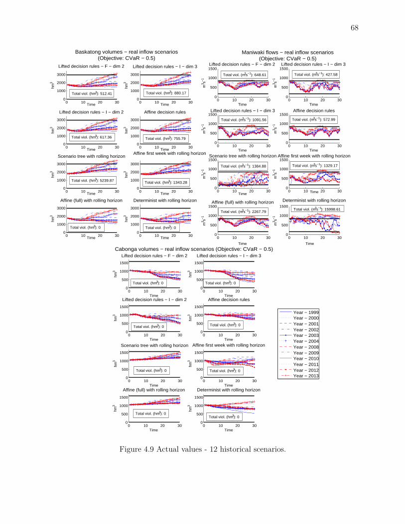
68

0 10 20 300

1000

2000

3000

Time

hm3

Lifted decision rules − F − dim 2

0 10 20 300

1000

2000

3000

Time

hm3

Lifted decision rules − I − dim 3

0 10 20 300

1000

2000

3000

Time

hm3

Lifted decision rules − I − dim 2

0 10 20 300

1000

2000

3000

Time

hm3

Affine decision rules

0 10 20 300

1000

2000

3000

Time

hm3

Scenario tree with rolling horizon

0 10 20 300

1000

2000

3000

Time

hm3

Affine first week with rolling horizon

0 10 20 300

1000

2000

3000

Time

hm3

Affine (full) with rolling horizon

Baskatong volumes − real inflow scenarios (Objective: CVaR − 0.5)

0 10 20 300

1000

2000

3000

Time

hm3

Determinist with rolling horizon

Total viol. (hm3): 0 Total viol. (hm3): 0

Total viol. (hm3): 5239.87 Total viol. (hm3): 1343.28

Total viol. (hm3): 755.79Total viol. (hm3): 617.36

Total viol. (hm3): 512.41 Total viol. (hm3): 880.17

0 10 20 300

500

1000

Lifted decision rules − F − dim 21500

m3 s−1

0 10 20 300

500

1000

1500

m3 s−1

Lifted decision rules − I − dim 3

0 10 20 300

500

1000

1500

m3 s−1

Time

Lifted decision rules − I − dim 3

0 10 20 300

500

1000

1500

m3 s−1

0 10 20 300

500

1000

Time

Scenario tree with rolling horizon1500

m3 s−1

0 10 20 300

500

1000

1500

1m

3 s−

Time

Affine first week with rolling horizon

0 10 20 300

500

1000

1500

Time

m3 s−1

Time

Affine (full) with rolling horizon

Maniwaki flows − real inflow scenarios (Objective: CVaR − 0.5)

0 10 20 300

500

1000

1500

Time

m3 s−1

Time

Determinist with rolling horizon

Total viol. (m3s−1): 1329.17

Total viol. (m3s−1): 427.58

Time

Affine decision rules

Total viol. (m3s−1): 572.99

Total viol. (m3s−1): 15998.61Total viol. (m3s−1): 2267.79

Total viol. (m3s−1): 1384.88

Total viol. (m3s−1): 1091.56

Total viol. (m3s−1): 648.61

0 10 20 300

500

1000

1500

hm3

Lifted decision rules − F − dim 2

0 10 20 300

500

1000

1500

hm3

Lifted decision rules − I − dim 3

0 10 20 300

500

1000

1500

hm3

TimeLifted decision rules − I − dim 2

0 10 20 300

500

1000

1500

hm3

TimeAffine decision rules

0 10 20 300

500

1000

1500

hm3

Time

Scenario tree with rolling horizon

0 10 20 300

500

1000

1500

hm3

Time

Affine first week with rolling horizon

0 10 20 300

500

1000

1500

Time

hm3

TimeAffine (full) with rolling horizon

Cabonga volumes − real inflow scenarios (Objective: CVaR − 0.5)

0 10 20 30

500

1000

1500

Time

hm3

TimeDeterminist with rolling horizon

0

Year − 1999Year − 2000Year − 2001Year − 2002Year − 2003Year − 2004Year − 2008Year − 2009Year − 2010Year − 2011Year − 2012Year − 2013

Total viol. (hm3): 0

Total viol. (hm3): 0

Total viol. (hm3): 0

Total viol. (hm3): 0

Total viol. (hm3): 0

Total viol. (hm3): 0

Total viol. (hm3): 0

Total viol. (hm3): 0

Figure 4.9 Actual values - 12 historical scenarios.

69

4.6.8 Brief comparison of budgeted and box uncertainty

We also tested our model with the following commonly use budgeted uncertainty set (seenamely Ardestani-Jaafari and Delage (2014)) 6 :

ζ ∈ RT

∣∣∣∣∣∣ ∃(ζ+>, ζ−>)> ∈ Zν,Γ

ζt′ = ζ+t′ − ζ−t′ ,∀t′

(4.21a)(4.21b)

where :

Zν,Γ =

(ζ+>, ζ−>)> ∈ R2T

+

∣∣∣∣∣∣∣∣∣∣∣∣∣

ζ+t′ ≤ νσt′ , ∀t′

ζ−t′ ≤ minµt′ , νσt′, ∀t′T∑t′=1

ζ+t′

νσt′+ ζ−t′

minµt′ , νσt′≤ Γ

(4.22a)(4.22b)

(4.22c)

Constraints (4.22a)-(4.22b) correspond to the basic box constraints, equality (4.21b) ensureswe get the original ζt and can be seen as the retraction operator while (4.22c) is the budgetconstraint determining the number of random variables that can take their extremal valuesover the entire horizon. To focus the comparison on the geometry of the uncertainty set ratherthan the power of the liftings, we fixed the coefficients of ζ+

t′ and ζ−t′ at the same value in theaffine decision rules (see 4.9.2 of the Appendix for more details).

Figure 4.10 suggests that there is not a significant difference between the performance of theaffine decision rules with and without the budget constraint with Γ > 0 when consideringindependent log-normally distributed random variables. In this case, the graphs of the em-pirical CVaR of the total violation cross and we cannot identify a dominant policy. This istrue for all budgets except for the case Γ = 0 which performs very poorly and is dominatedby all policies. As intuition might suggest, the policy considering only box support hedgesagainst very extreme scenarios. As such, it does better in the worst case, but at the priceof degraded CVaRα′ performance compared to the policy with the budget constraint withΓ > 0 for α′ ∈ (0, 100].

However, when we consider the seasonal time series model with strong correlation acrosstime, we find more significant variations in performance across policies. We namely see thatconsidering Γ ≤

√T ≈ 5.48 leads to poor results with empirical risk higher than the one of

the box support for all α′ ∈ [0, 100]. In this case, the budgeted uncertainty set fails to take

6. For all experiments with the budgeted uncertainty set, we fixed ν = 3 as in the rest of our numericalexperiments.

70

into account the possibility of persistently high or low inflows. For Γ =√T + i (T−

√T )

5 andi ∈ 1, 2, 3, 4, 5 however, neither the box nor the policy with the budget dominate the other.Only i = 5 is shown in Figure 4.10, but the results are very similar for i ∈ 1, 2, 3, 4. As inthe independent case, the box leads to better worst case performance, but degraded CVaRα′

performance for α′ ∈ (0, 100].

It is also interesting to note that although the theoretical models with the box and the non-binding budget constraint with Γ = 30 are equivalent, the solutions found and the simulationresults differ. This is another consequence of the multiplicity of the optimal solutions and thedegeneracy of the problem. Solutions with the same objective value can yield different resultswhen tested against specific scenarios. In future work, it may be interesting to consider mul-tiple objectives to resolve this multiplicity. For instance, we could compare different optimalsolutions obtained by minimizing a fixed CVaRα based on their performance for differentCVaRα′ .

0 20 40 60 80 100

103

104

105

Empirical Total violations (CVaR − 0.5)(Affine)(Log Normal)

α′

CV

aRα′

(hm

3 )

0 20 40 60 80 100

104

105

Empirical Total violations (CVaR − 0.5)(Affine)(SARIMA)

α′

CV

aRα′

(hm

3 )

BoxBudget − Γ=0 Budget − Γ=5.48 Budget − Γ=6.70 Budget − Γ=7.93 Budget − Γ=30

Student Version of MATLAB

Figure 4.10 Impact of different uncertainty sets on simulation results.

Computational experiments also revealed that by considering the budgeted uncertainty setwith Γ = T so that the constraint is not binding, the computational time grew from 3.9minutes with our standard box formulation to 153.9 minutes (≈ 2.5 hours) with the budgeteduncertainty sets when considering the ess sup as the risk measure. This is an increase of morethan 39 times.

Table 4.5 sheds light on this initially surprising result. We first observe that the budgetedformulation generates T additional inequalities and equalities for each inequality in the ori-

71

ginal deterministic formulation. We then note that the robust equivalents have very differentstructure. The robust equivalent of the box model generates significantly more equalities thaninequalities. This is a consequence of the dualization procedure and is described explicitly inSections 4.9.1 and 4.9.2 of the Appendix. The consequences of this large number of equalitiesis that the presolve engine of both AMPL and CPLEX can make dramatic reductions inmodel size by appropriate substitutions. Turning this option off namely resulted in muchlarger models and increased computing times with the box support.

Tableau 4.5 Size of robust equivalents (box vs. budget).

Standard affine (box support) Standard affine (budget support)# constraints (rob. model) # (dual) variables

(rob. model)# constraints (rob. model) # (dual) variables

(rob. model)Equalities Inequalities Equalities InequalitiesInequality

(Det. model) T 1 2T - 2T+1 2T+1

Equality(Det. model) T+1 - - T+1 - -

To validate these results, we also tested the following equivalent uncertainty set :

ζ ∈ RT

∣∣∣∣∣∣∣∣∣∣∣∣∣∣∣∣∣∣∣∣

∃% ∈ RT+

ζt′ ≤ %t′νσt′ , ∀t′

− ζt′ ≤ %t′ minµt′ , νσt′, ∀t′

%t′ ≤ 1, ∀t′

T∑t′=1

%t′ ≤ Γ

(4.23a)(4.23b)(4.23c)(4.23d)

(4.23e)

Contrary to formulation (4.21), the ζt are unrestricted in sign in (4.23). This uncertaintyset therefore leads to the same number of equalities as the box, but with an additional Tinequalities for each original inequality. Considering this alternative formulation reduced thecomputing times by a factor close to 4 compared with formulation (4.21) for tests performedwith CVaRα and α ∈ 0, 0.5, 1. However, when setting Γ ≥ T , the standard box still perfor-med significantly better than both budgeted formulations in terms of computing times. Thesefindings corroborate the importance of the number of equalities in the resulting deterministicequivalent.

Nonetheless, Figure 4.11 shows that the model with budgeted uncertainty can provide betterquality policies than those of the standard box for fixed scenarios. Indeed, if we consider the12 historical inflow scenarios and use Γ =

√T + 2 (T−

√T )

5 ≈ 15.29, which is very close to15.90, the minimal value that ensures that all 6 years of real data are contained within the

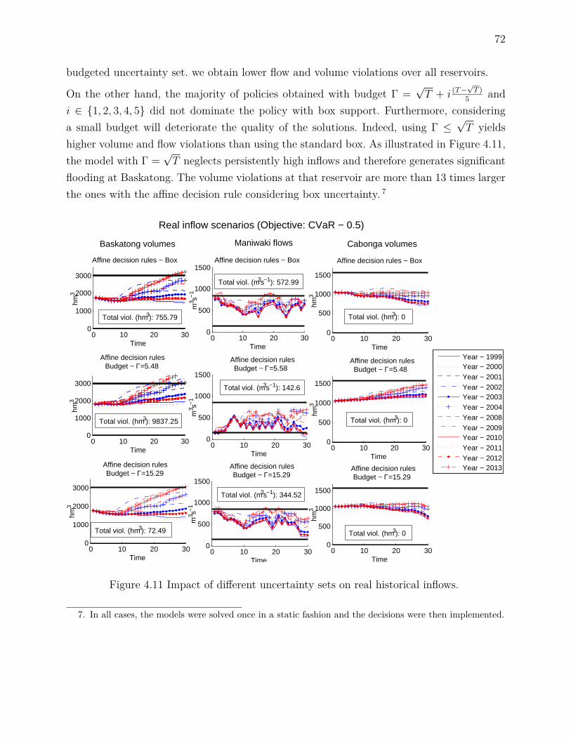
72

budgeted uncertainty set. we obtain lower flow and volume violations over all reservoirs.

On the other hand, the majority of policies obtained with budget Γ =√T + i (T−

√T )

5 andi ∈ 1, 2, 3, 4, 5 did not dominate the policy with box support. Furthermore, consideringa small budget will deteriorate the quality of the solutions. Indeed, using Γ ≤

√T yields

higher volume and flow violations than using the standard box. As illustrated in Figure 4.11,the model with Γ =

√T neglects persistently high inflows and therefore generates significant

flooding at Baskatong. The volume violations at that reservoir are more than 13 times largerthe ones with the affine decision rule considering box uncertainty. 7

0 10 20 300

1000

2000

3000

Time

hm3

Affine decision rules − Box

0 10 20 300

1000

2000

3000

Time

hm3

Affine decision rules Budget − Γ=5.48

0 10 20 300

1000

2000

3000

Time

hm3

Affine decision rules Budget − Γ=15.29

0 10 20 300

500

1000

1500

Time

m3 s−

1

Affine decision rules − Box

0 10 20 300

500

1000

1500

Time

m3 s−

1

Affine decision rulesBudget − Γ=5.58

0 10 20 300

500

1000

1500

Time

m3 s−

1

Affine decision rules Budget − Γ=15.29

0 10 20 300

500

1000

1500

Time

hm3

Affine decision rules − Box

0 10 20 300

500

1000

1500

Time

hm3

Affine decision rulesBudget − Γ=5.48

Real inflow scenarios (Objective: CVaR − 0.5)

0 10 20 300

500

1000

1500

Time

hm3

Affine decision rulesBudget − Γ=15.29

Year − 1999Year − 2000Year − 2001Year − 2002Year − 2003Year − 2004Year − 2008Year − 2009Year − 2010Year − 2011Year − 2012Year − 2013

Total viol. (hm3): 0

Total viol. (hm3): 0

Total viol. (hm3): 0

Total viol. (m3s−1): 572.99

Total viol. (m3s−1): 142.6

Total viol. (m3s−1): 344.52

Total viol. (hm3): 755.79

Total viol. (hm3): 9837.25

Total viol. (hm3): 72.49

Baskatong volumes Maniwaki flows Cabonga volumes

Student Version of MATLAB

Figure 4.11 Impact of different uncertainty sets on real historical inflows.

7. In all cases, the models were solved once in a static fashion and the decisions were then implemented.

73

4.7 Conclusion

In conclusion, we propose a novel robust optimization formulation for the risk averse sto-chastic reservoir management problem. Our model can easily be obtained from an existingdeterministic model and is relatively easy to understand and implement.

We also formalize risk-aversion through the coherent risk measure CVaRα. By performingsensitivity analysis on the α parameter, we study the theoretical and simulated impact ofdifferent risk profiles.

Contrary to other popular methods such as stochastic dynamic programming, we can easilyincorporate constraints involving different time steps, such as flow variation constraints. Ourmethod also allows the consideration of objective functions such as CVaR that do not permittime decomposition.

Our various numerical experiments confirm the value of using affine decision rules to providegood implementable solutions while maintaining the tractability of the model. Our experi-ments also suggest that these decision rules offer little optimality loss over more complexpiece-wise linear decision rules while providing extremely important computational savings.Affine and piece-wise linear decision rules seem to perform consistently better than decisiontrees, even when considering a rolling horizon framework.

The results based on historical and synthetic inflows also suggest that the affine decision rulescompare favourably with scenario tree models in terms of solution quality. However, theseconclusions may not be generalizable to other problems and instances. In addition, moreelaborate and representative scenario trees may lead to better results, since these modelcan exploit probabilities and serial correlation to which the robust model is insensitive. Ourintuition is that if the decision makers have very rich and reliable data spanning long timeperiods, then it might be beneficial to exploit the structure provided by scenario trees. Onthe other hand, if the decisions makers only have limited data, as was the case in this study,or if they must extrapolate into the future and stationarity is a questionable assumption,then the robust model may provide more reliable results.

Our experiments also showcase the computational advantages of the affine decision rulescompared to the tree based model. We feel that this is an important point, notably foroperational purposes. This advantage may be less important if the model is only used forstrategic long term decisions and long computing times are acceptable. Nonetheless, detailedtree structures will invariably lead to difficulties when using simulation and stress tests. Itmight be possible to speed up computations by using decomposition techniques such as theones considered in Carpentier et al. (2013a), however, these will require a significantly amount

74

of technical work to implement.

Finally, we perform a brief but interesting comparison of box and budgeted uncertainty sets.We show that in the presence of significant serial correlation, decision makers should usecaution when choosing the value of Γ. If the model can be calibrated thorough reliable simu-lation, then it might be preferable to consider the budget uncertainty sets with a properlychosen budget. However, in the context of considerable ambiguity in distributions and possi-bly non-stationary, the simple box might provide more reliable solutions. In any case, the useof the box uncertainty set should reduce model size and speed up computations comparedwith the budgeted uncertainty set.

4.8 Acknowledgments

The authors would like to thank everyone at Hydro-Québec and IREQ for their ongoingsupport, particularly Grégory Émiel, Louis Delorme and Pierre-Marc Rondeau as well asPierre-Luc Carpentier and Alexia Marchand. We are also grateful to Daniel Kuhn, PascalCôté and Sara Séguin for valuable discussions. The comments of anonymous referees also hel-ped improve the quality of the paper. This research was supported by the Natural Sciencesand Engineering Reasearch Council of Canada (NSERC) and Hydro-Québec through the In-dustrial Research Chair on the Stochastic Optimization of Electricity Generation and NSERCgrant 386416-2010 .

4.9 Appendix

4.9.1 Representative robust constraint under standard affine decision rules andbox uncertainty

Consider standard affine decision rules and the maximum turbined flow constraints (4.7) :Rit(ζ) ≤ ri,∀ζ ∈ Zν = T

t=1[−minµt, νσt, νσt] for a fixed plant and time. We omit theindices i and t for sake of clarity and formulate these robust constraints as the followinglinear program :

maxζ

R0 +T∑t′=1Rt′ζt′ ≤ r

s. t. (π+t′ ) ζt′ ≤ νσt′ , ∀t′ = 1, · · · , T

(π−t′ ) − ζt′ ≤ −minµt′ , νσt′, ∀t′ = 1, · · · , T

75

Taking the dual yields :

minπ

R0 +T∑t′=1

[νσt′π

+t′ −minµt′ , νσt′π−t′

]≤ r

s. t. π+t′ − π+

t′ = Rt′ , ∀t′ = 1, · · · , Tπ+t′ , π

−t′ ≥ 0, ∀l′ = 1, · · · , L

4.9.2 Representative robust constraint under standard affine decision rules andbudgeted uncertainty

In contrast, adding a budget constraint with budget Γ > 0 to our basic box uncertainty yieldsthe following linear program :

maxζ

R0 +T∑t′=1Rt′(ζ+

t′ − ζ−t′ ) ≤ r

s. t. (π+t′ ) ζ+

t′ ≤ νσt′ , ∀t′ = 1, · · · , T(π−t′ ) ζ−t′ ≤ minµt′ , νσt′, ∀t′ = 1, · · · , T

(π0)T∑t′=1

ζ+t′

νσt′+ ζ−t′

minµt′ , νσt′≤ Γ

ζ+t′ , ζ

−t′ ≥ 0, ∀t′ = 1, · · · , T

Taking the dual yields :

minπ

R0 +T∑t′=1

[νσt′π

+t′ + minµt′ , νσt′π−t′

]+ Γπ0 ≤ r

s. t. π+t′ + π0

νσt′≥ Rt′ , ∀t′ = 1, · · · , T

π−t′ + π0

minµt′ , νσt′≥ −Qt′ , ∀t′ = 1, · · · , T

π+t′ , π

−t′ ≥ 0, ∀l′ = 1, · · · , L

Note that since the intervals [minµt, νσt, νσt] may be non symmetric for any t, we have toconsider the problem on the lifted space with ζt = ζ+

t − ζ−t decomposed into its positive and

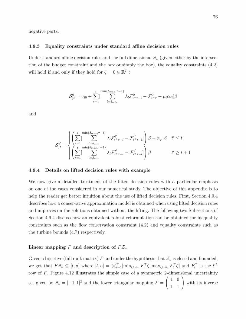
76

negative parts.

4.9.3 Equality constraints under standard affine decision rules

Under standard affine decision rules and the full dimensional Zν (given either by the intersec-tion of the budget constraint and the box or simply the box), the equality constraints (4.2)will hold if and only if they hold for ζ = 0 ∈ RT :

S0jt = vj0 +

t∑τ=1

[minδmax,τ−1∑

l=δminλlF0

i+τ−l −F0i−τ + µtαjt]β

and

St′jt =

t∑τ=1

[minδmax,τ−1∑

l=δminλlF t

′

i+τ−l −F t′

i+τ−l] β + αjt′β t′ ≤ t t∑

τ=1[minδmax,τ−1∑

l=δminλlF t

′

i+τ−l −F t′

i+τ−l] β t′ ≥ t+ 1

4.9.4 Details on lifted decision rules with example

We now give a detailed treatment of the lifted decision rules with a particular emphasison one of the cases considered in our numerical study. The objective of this appendix is tohelp the reader get better intuition about the use of lifted decision rules. First, Section 4.9.4describes how a conservative approximation model is obtained when using lifted decision rulesand improves on the solutions obtained without the lifting. The following two Subsections ofSection 4.9.4 discuss how an equivalent robust reformulation can be obtained for inequalityconstraints such as the flow conservation constraint (4.2) and equality constraints such asthe turbine bounds (4.7) respectively.

Linear mapping F and description of FZν

Given a bijective (full rank matrix) F and under the hypothesis that Zν is closed and bounded,we get that FZν ⊆ [l, u] where [l, u] = T

t=1[minζ∈Zν F>t ζ,maxζ∈Zν F>t ζ] and F>t is the tth

row of F . Figure 4.12 illustrates the simple case of a symmetric 2-dimensional uncertainty

set given by Zν = [−1, 1]2 and the lower triangular mapping F = 1 0

1 1

with its inverse

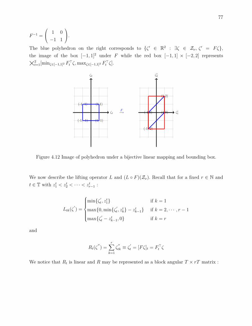
77

F−1 = 1 0−1 1

.The blue polyhedron on the right corresponds to ζ ′ ∈ R2 : ∃ζ ∈ Zν , ζ ′ = Fζ,the image of the box [−1, 1]2 under F while the red box [−1, 1] × [−2, 2] represents2

t=1[minζ∈[−1,1]2 F>t ζ,maxζ∈[−1,1]2 F

>t ζ].

ζ1

ζ2

(-1, 1)

(-1, -1) (1,-1)

(1,1)

Fζ ′1

ζ ′2

(-1,-2)

(1,0)

(1,2)

(-1,0)

Figure 4.12 Image of polyhedron under a bijective linear mapping and bounding box.

We now describe the lifting operator L and (L F )(Zν). Recall that for a fixed r ∈ N andt ∈ T with zt1 < zt2 < · · · < ztr−1 :

Ltk(ζ′) =

minζ ′t , zt1 if k = 1

max0,minζ ′t , ztk − ztk−1 if k = 2, · · · , r − 1

maxζ ′t − ztk−1, 0 if k = r

and

Rt(ζ′′) =

r∑k=1

ζ′′

tk ≡ ζ′

t = [Fζ]t = F>t ζ

We notice that Rt is linear and R may be represented as a block angular T × rT matrix :

78

R =

1 · · · 1︸ ︷︷ ︸r terms

1 · · · 1. . .

. . .1 · · · 1

As described in Georghiou et al. (2015), in order to get an accurate description of the uncer-tainty set for ζ ′′, we need to characterize the convex hull of (LF )(Zν). Geoghiou et al. showhow this can be done exactly when F (Zν) is an hyperrectangle. In particular, if one conside-red the lifted image L(t[lt, ut]), then he could exploit the property that conv(L(t[lt, ut]))= t convLt([lt, ut]) and observe that for every t, Lt([lt, ut]) is a set of connected segments(defined through the choice of breakpoints zt1, · · · , ztr−1) for which convLt([lt, ut]) simply re-duces to the set of convex combinations of the following r + 1 affinely independent points inRr :

vt1 =

lt

0· · ·0

vt2 =

zt1

0· · ·0

vt3 =

zt1

zt2 − zt1· · ·0

· · · vtr+1 =

zt1

zt2 − zt1· · ·

ut − ztr−1

For instance, consider the simple lifting which breaks the components into their positive andnegative parts. We have r = 2, z1

1 = z12 = 0 and l1 = −1, u1 = 1, l2 = −2, u2 = 2. This is

illustrated in Figure 4.13 where the solid green lines indicate Lt([lt, ut]) and the (light andsolid) green represents conv(Lt([lt, ut])).

ζ ′′21

ζ ′′22

(-2, 0) (0, 0)

(0,2)

ζ ′′11

ζ ′′12

(-1,0) (0,0)

(0,1)

Figure 4.13 Lt([lt, ut]) and conv(Lt([lt, ut])), t = 1, 2.

79

If we regroup the points vt1, vt2, · · · , vtr+1 in the following invertible matrix :

Vt = 1 · · · 1vt1 · · · vtr+1

∈ R(r+1)×(r+1)

then we have :

convLt([lt, ut]) = ζ ′′t ∈ Rr : (1, ζ ′′>t )> = Vtλ, λ ∈ Rr+1+

= ζ ′′t ∈ Rr : V −1t (1, ζ ′′>t )> ≥ 0.

Building on these observations, we obtain :

conv(L F )(Zν) = conv((L F )(Zν) ∩ ζ ′′ ∈ RrT : ∃ζ ∈ Zν , Rζ ′′ = Fζ) (4.24)⊆ conv((L F )(Zν)) ∩ conv(ζ ′′ ∈ RrT : ∃ζ ∈ Zν , Rζ ′′ = Fζ) (4.25)⊆ conv(L(

t

[lt, ut])) ∩ conv(ζ ′′ ∈ RrT : ∃ζ ∈ Zν , Rζ ′′ = Fζ) (4.26)

= Z ′′ν := ζ ′′ ∈ RrT : F−1Rζ ′′ ∈ Zν , V −1t ζt

′′ ≥ 0,∀t , (4.27)

where the first inclusion comes from the property that conv(A ∩ B) ⊆ conv(A) ∩ conv(B),while the second inclusion comes from the property that FZν ⊆

t[lt, ut] which implies

that conv((L F )(Zν)) ⊆ conv(L(t[lt, ut])). We will conveniently formulate each robustconstraint of the lifted decision rules model in terms of Z ′′ν .

Following our previous example with r = 2, we see that V −1t ζt

′′ ≥ 0,∀t corresponds to :

0 1

lt0

1 − 1lt− 1ut

0 0 1ut

︸ ︷︷ ︸

V −1t

1ζ ′′t1

ζ ′′t2

≥

000

, t = 1, 2 (4.28)

⇔ ζ ′′21 ≤ 0 ζ ′′11 ≤ 0 (4.29)−ζ ′′21

2 + ζ ′′222 ≤ 1 − ζ ′′11 + ζ ′′12 ≤ 1 (4.30)

ζ ′′22 ≥ 0 ζ ′′12 ≥ 0 (4.31)

80

with ζ ′1 = R1ζ′′ = ζ11 + ζ12 and ζ ′2 = R1ζ

′′ = ζ21 + ζ22 where we could use the more eloquentlabelling ζt1 = −ζ−t ≤ 0 and ζt2 = ζ+

t ≥ 0 for t = 1, 2 to represent the negative and positivepart of ζ ′t. At any extreme point of Z ′′ν , at most one of ζ ′′t1 or ζ ′′t2 can be non-zero for t = 1, 2.From (4.27), all that is left is to ensure F−1Rζ ′′ ∈ Zν . In our example, this translates to Z ′′νbeing described with the following linear constraints :

−1−1

≤ 1 0−1 1

︸ ︷︷ ︸

F−1

1 1 0 00 0 1 1

︸ ︷︷ ︸

R

ζ ′′11

ζ ′′12

ζ ′′21

ζ ′′22

≤ 1

1

and (4.29)− (4.31). (4.32)

It is worth emphasizing the fact that since Z ′′ν is an outer approximation of conv(L F )(Zν),one should expect that each robust constraint will be replaced by one that is more conservativethan needed hence preventing the optimization model from fully exploiting the flexibilityprovided by the piecewise linear lifting. However, with Z ′′ν , we are at least guaranteed toobtain a better approximation than with the scheme that only uses affine decision rules. Thisis due to the fact that for any standard and lifted affine decision rules of the form (4.13) and(4.20), respectively :

Xkt(ζ) = X 0kt +

T∑t′=1X t′

ktζt′ , k ∈ Kt

Xkt(ζ ′′) = X 0kt +

T∑t′=1

r∑s=1X t′skt ζ

′′t′,s k ∈ Kt

it is always possible to fix the values X t′skt to ensure that the following holds for a fixed affine

policy and an arbitrary function f : R× RT → R :

maxζ∈Zν

f(Xkt(ζ), ζ) = maxζ′′∈RrT :F−1Rζ′′∈Zν

f(Xkt(ζ ′′), F−1Rζ ′′)

≥ maxζ′′∈Z′′ν

f(Xkt(ζ ′′), F−1Rζ ′′) ,

The equality follows from the particular restriction of the lifted decision rules and the factthat the "retracted" F−1Rζ ′′ lie within Zν . For instance, with the identity mapping F = I,it suffices to set X t′s

kt = X t′kt,∀s ∈ 1, · · · , r, since

∑rs=1 ζ

′′t′,s = ζt′ for any t′. The inequality

81

follows from equation (4.27), which implies Z ′′ν ⊆ ζ ′′ ∈ RrT : F−1Rζ ′′ ∈ Zν. We thereforeconclude that for any feasible solution based on standard affine decision rules it is possibleto find a feasible solution with lifted decision rules with the same objective value.

The following subsections will illustrate how we can derive a reformulation for each typeof robust constraint in this lifted decision rules framework under Z ′′ν as defined in equation(4.32).

Representative robust constraint under lifted decision rules

Under the lifting (LF ) where F is linear and bijective, the robust turbined flow constraints(4.7) for a fixed plant i and time t will be satisfied by imposing maxζ′′∈Z′′ν⊇(LF )(Zν)R0 +∑Tt=1

∑rj=1Rtjζ ′′tj ≤ r.

We let at represent the 1st column of V −1t and bt ∈ R(r+1)×r be the matrix composed of the

last r columns of V −1t from the preceding Section 4.9.4. We can then write this explicitly as

the following linear program with block constraint matrix under the hypothesis that Zν =Tt=1[minµt, νσt, νσt] :

R0 + maxζ′′

R11ζ′′11+ ... +R1rζ

′′1r+ ... RT1ζ

′′T1+ ... +RTrζ

′′Tr ≤ r

s. t. (π+1 ) F−1

11 ζ′′11 ... F−1

11 ζ′′1r ... F−1

1T ζ′′T1 ... F−1

1T ζ′′Tr ≤ νσ1

(π+2 ) F−1

21 ζ′′11 ... F−1

21 ζ′′1r ... F−1

2T ζ′′T1 ... F−1

2T ζ′′Tr ≤ νσ2

... ... ... ... ... ... ... ... ...

(π+T ) F−1

T1 ζ′′11 ... F−1

T1 ζ′′1r ... F−1

TT ζ′′T1 ... F−1

TT ζ′′Tr ≤ νσT

(π−1 ) −F−111 ζ

′′11 ... −F−1

11 ζ′′1r ... −F−1

1T ζ′′T1 ... F−1

1T ζ′′Tr ≤ minµ1, νσ1

(π−2 ) −F−121 ζ

′′11 ... −F−1

21 ζ′′1r ... −F−1

2T ζ′′T1 ... −F−1

2T ζ′′Tr ≤ minµ2, νσ2

... ... ... ... ... ... ... ... ...

(π−T ) −F−1T1 ζ

′′11 ... −F−1

T1 ζ′′1r ... −F−1

TT ζ′′T1 ... −F−1

TT ζ′′Tr ≤ minµT , νσT

(φ11) −b111ζ

′′11 ... −b1

1rζ′′1r ≤ a1

1

... ... ... ...

(φ1(r+1)) −b1(r+1)1ζ

′′11 ... −b1

(r+1)rζ′′1r ≤ a1

(r+1)

... ... ... ... ... ... ... ... ...

(φT1) −bT11ζ′′T1 ... −bT1rζ

′′Tr ≤ aT1

... ... ... ...

(φT (r+1)) −bT(r+1)1ζ′′T1 ... −bT(r+1)rζ

′′Tr ≤ aTr+1

82

The first set of constraints associated with the π dual variables represent F−1Rζ ′′ ∈ Zν whenZν = T

t=1[max−νσt,−µt, νσt] and the second one associated with the φ dual variablesrepresents V −1

t (1, ζ ′′t1, · · · , ζ ′′tr)> ≥ (0, · · · , 0)>,∀t. Taking the dual yields :

R0 + minπ,φ

T∑t′=1

(νσt′π+t′ + π−t′ minµt′ , νσt′) +

T∑t′=1

r+1∑j′=1

φt′j′at′

j′ ≤ r

s. t.T∑

t′′=1F−1t′′t′(π+

t′′ − π−t′′)−r+1∑j′′=1

φt′j′′bt′

j′′j′ = Rt′j′ ∀t′ = 1, · · · , T, j′ = 1, · · · , r

π−t′ , π−t′ ≥ 0 ∀t′ = 1, · · · , T

φt′j′′ ≥ 0, ∀t′ = 1, · · · , T, j′′ = 1, · · · , r + 1

Equality constraints under lifted affine decision rules

Under the lifted decision rules, the nominal equality constraints for ζ = 0 remain the same :

S0jt = vj0 +

t∑τ=1

[minδmax,τ−1∑

l=δminλlF0

i+τ−l −F0i−τ + µταjτ ]β

However, the other constraints take the form :

Sj′t′

jt = t∑τ=1

[minδmax,τ−1∑

l=δminλlF t

′j′

i+τ−l −Ft′j′

i+τ−l + F−1τt′ αjτ ]

βfor all t′ = 1, · · · , T, j′ = 1, · · · , r, t = 1, · · · , T and j ∈ J . In particular, if F = I, thenF−1τt = 1 if τ = t and 0 otherwise, which yields a structure similar to the standard affine case.

83

CHAPITRE 5 ARTICLE 2: A STOCHASTIC PROGRAM WITH TIMESERIES AND AFFINE DECISION RULES FOR THE RESERVOIR

MANAGEMENT PROBLEM

Cet article a été accepté avec révision mineures par European Journal of Operational Researchen avril 2017. Auteurs : Charles Gauvin, Erick Delage et Michel Gendreau.

Un rapport technique préliminaire est disponible : Gauvin, C., Delage, E. et Gendreau, M.,A stochastic program with time series and affine decision rules for the reservoir managementproblem, Les Cahiers du GERAD, Avril 2016, Révisé Janvier 2017, ISSN : 0711–2440 (Gauvinet al., 2016).

Abstract : This paper proposes a multi-stage stochastic programming formulation for thereservoir management problem. Our problem specifically consists in minimizing the risk offloods over a fixed time horizon for a multi-reservoir hydro-electrical complex. We considerwell-studied linear time series models and enhance the approach to consider heteroscedas-ticity. Using these stochastic processes under very general distributional assumptions, weefficiently model the support of the joint conditional distribution of the random inflows andupdate these sets as new data are assimilated. Using robust optimization techniques andaffine decision rules, we embed these time series in a tractable convex program. This allowsus to obtain good quality solutions rapidly and test our model in a realistic simulation fra-mework using a rolling horizon approach. Finally, we study a river system in western Québecand perform various numerical experiments based on different inflow generators.

Keywords : Stochastic programming, Stochastic processes, Robust optimization, Forecas-ting, OR in energy, Risk analysis

5.1 Introduction

This paper considers the problem of minimizing the risk of floods for a multi-reservoir systemover a fixed time horizon subject to uncertainty on inflows while respecting tight operationalconstraints on total storage, spills, releases, water balance and additional physical constraints.This reservoir management problem is of vital importance to various real sites that are closeto human habitations and that are prone to flooding (Quentin et al., 2014; Pianosi andSoncini-Sessa, 2009; Castelletti et al., 2010; Gauvin et al., 2017).

The deterministic version of the problem already poses serious challenges since operatorsmust consider complex non-linear phenomena related to the physical nature of the system

84

(Labadie, 2004). The interconnection of the catchment also complicates decisions as ups-tream releases affect downstream volumes and flows. This issue is particularly important forlarge catchments where there can be long water delays (Gauvin et al., 2017). Considering un-certainty significantly increases theses difficulties since the sequential decision-making underuncertainty represents a huge theoretical obstacle in itself (Dyer and Stougie, 2006).

In order to solve this problem, we propose a multi-stage stochastic program based on affinedecision rules and well-known time series models. Our approach leverages techniques fromstochastic programming, stochastic processes and robust optimization.

Starting with the pioneering work of Ben-Tal et al. (2004), adjustable robust optimizationbased on affine decision rules has emerged as a viable approach for dynamic problems whereuncertainty is progressively revealed. The approach has been shown capable of finding goodquality solutions to large multi-stage stochastic problems that would otherwise be unmana-geable to traditional methods such as stochastic dynamic programming.

These techniques have been applied to the reservoir management problems with a varyingdegree of success. The authors of Apparigliato (2008) and Pan et al. (2015) use this frameworkto maximize the expected electric production for a multi-period and multi-reservoir hydro-electric complex while Gauvin et al. (2017) minimize the risk of floods by adopting a riskaverse approach that explicitly considers the multidimensional nature of the problem subjectto more realistic operating constraints.

Although some of these studies use elaborate decision rules based on works such as Chen et al.(2008); Goh and Sim (2010) and Georghiou et al. (2015), they only consider very simplifiedrepresentations of the underlying stochastic process and generally omit serial correlation.However, the importance of the persistence of inflows can play a crucial factor in hydrologicalmodelling for stochastic optimization problems, particularly when daily inflows need to beconsidered. Authors like Turgeon (2005); Pianosi and Soncini-Sessa (2009) argue that serialcorrelation of high order is important to consider inflows that are high or low on manyconsecutive days and risk producing a flood or low baseflow.

This paper addresses the issue by developing a dynamic robust uncertainty set that takesinto consideration the dynamic structure and serial correlation of the inflow process. We showthat under certain conditions, these sets correspond to the support of the joint conditionaldistribution of uncorrelated random variables that determine the inflows over a given horizon.Our work shares similarities with the paper of Lorca and Sun (2015) who propose dynamicuncertainty sets based on time series models for a 2-stage economic dispatch problem in thepresence of high wind penetration. Like these authors, we take advantage of the dynamicadaptability of the uncertainty sets by incorporating our model in a realistic simulation

85

framework with rolling horizon.

Nonetheless, we give significantly more details on the construction of these uncertainty sets forgeneral univariate ARMA models and provide key insights which are of value to practitionersand academics alike. We also consider the case of heteroscedasticity which is empiricallyobserved in various inflow time series (Romanowicz et al., 2006). Although we minimize therisk of floods, our work can be directly extended to electricity generation, under the hypothesisthat head is constant and that the production function can be modeled as a piecewise linearfunction.

Our model considers ARMA and GARCH models of any order without increasing the com-plexity of the problem. This is a huge improvement over stochastic dynamic programming(SDP) methods, which have historically been the most popular techniques used for reservoirmanagement both in academia and in practice (see Labadie (2004); Yeh (1985); Castellettiet al. (2008); Turgeon (2005) and references therein). Although these methods can deal withmore realistic non-convex optimization problems and provide excellent closed-loop policies,they can usually only consider serial correlation through autoregressive models of small ordersince higher order models require increasing the state-space, which quickly leads to numeri-cal intractability ; particularly for multi-reservoir operations (Turgeon, 2007; Cervellera et al.,2006; Tilmant and Kelman, 2007).

Considering heteroscedasticity further increases the state dimension and the resulting compu-tational burden for SDP. As such, we are only aware of the work of Pianosi and Soncini-Sessa(2009) that is capable of considering this phenomenon with this methodology. Furthermore,these authors only manage to incorporate heteroscedasticity in a reduced model used foron-line computations.

Numerous refinements of classical SDP have emerged to circumvent some of these difficulties.Neuro-dynamic programming (Castelletti et al., 2010), sampling SDP (Stedinger and Faber,2001) and more elaborate discretization schemes (Zéphyr et al., 2016; Cervellera et al., 2006)have namely been applied successfully to large reservoir systems while explicitly or implici-tely considering high order serial correlation. However, most of these methods still requiresimplifications of the river dynamics and inflow representation as well as discretization ofdecisions, which is not the case of our approach.

Other works based on SDP, such as Turgeon (2005); Stedinger and Faber (2001); Tejada-Guibert et al. (1995); Côté et al. (2011), have focused on various low-dimensional hydrologicalvariables such as seasonal forecasts, additional exogenous information like soil moisture andlinear combinations of past inflows. Although these aggregate hydrological variables improvethe solution quality without excessive computational requirements, they often rely on distri-

86

butional assumptions such as normality that are not verified in practice or exogenous datathat may be difficult to obtain. Our model does not suffer from such limitations.

In recent years, the stochastic dual dynamic programming (SDDP) method has emerged asan effective algorithm capable of successfully tackling multi-dimensional stochastic reservoirsproblems (Tilmant and Kelman, 2007; Shapiro et al., 2013; Rougé and Tilmant, 2016; Gjels-vik et al., 2010; Pereira and Pinto, 1991; Phillpot and Guan, 2008). Moreover, Maceira andDamázio (2004) illustrate that this method can consider multiple lag autoregressive processeswithout excessively increasing the size of the problem for the aggregated 4-state Brazilianhydro-thermal system. However, the algorithm can exhibit relatively slow convergence (Sha-piro et al., 2013). To avoid this issue, various studies only consider a limited number ofdiscrete scenarios (<100) (Tilmant and Kelman, 2007; Rougé and Tilmant, 2016), but thisonly leads to approximate solutions of questionable quality (Shapiro, 2011).

We also mention stochastic programming methods based on decision trees, which are alsotheoretically capable of explicitly handling highly persistent inflows (Carpentier et al., 2013a;Gonçalves et al., 2013; Fleten et al., 2011). These models are simple to implement when anexisting deterministic model already exists and are intuitive to use and interpret. Unfor-tunately, they display exponential growth in complexity as a function of the time horizon.Therefore, they are usually limited to small decision trees. Gauvin et al. (2017) shows thatthese methods can be considerably more computationally intensive than corresponding sto-chastic programs based on decision rules.

The main advantage of our method with respect to SDDP and scenario-tree based stochasticprogram is its limited distributional assumptions. Whereas these competing methods requiresusing specific distributions from which it is possible to sample, our approach only demandshypothesis on the first 2 moments of the random variables as well as the correlation betweenthem. As observed by Pan et al. (2015), this is likely to lead to solutions that are more robustwhen tested on out-of-sample scenarios, which is of prime concern when data availability islimited. Another shortcoming of SDDP and tree-based stochastic programming comparedwith decision rules and SDP are their inability to provide explicit policies that can be directlyused by decision makers. Nonetheless, this is usually not a critical point, particularly whenrolling horizon simulations are considered.

The paper is structured as follows. The model for the deterministic reservoir managementproblem and the stochastic version based on affine decision rules are presented in Section5.2. Section 5.3 discusses inflow representation and general univariate ARMA models and theresulting conditional supports. It then studies heteroscedastic time series and their impact onthe model formulation. Section 5.4 explains the solution procedure and simulation framework

87

while Section 5.5 studies a river in western Québec. Conclusions are drawn in Section 5.6.

5.1.1 Notation

The sets Z+ = 0, 1, 2, · · · and Z− = 0,−1,−2, · · · represent the non-negative and non-positive integers while Sn+ is the cone of square n × n semi-definite matrices. The set T =1, · · · , T represents the entire horizon of T periods and L = 0, · · · , L − 1 denotes alimited look-ahead horizon for some L < T .

Let (Ω,F , Ft,P) be a filtered probability space where Ft is a collection of σ-algebrasrepresenting some information available at time t ∈ T where F0 = Ω, ∅ and FT = F . Welet E [·] denote mathematical expectation while E[·|A ] represents conditional expectationgiven any σ-algebra A ⊆ F . Both expectations are taken with respect to P, the baseprobability measure on F .

For the real random variables X, σ(X) represents the σ-algebra generated by X (Billingsley,1995). We abuse language and refer to the support of X as the smallest closed set on whichX takes values with probability one. For any discrete time real valued stochastic processXtt∈Z, we denote the RL valued random vector (Xt, · · · , Xt+L−1)> ≡ X[t,t+L−1] for anyt ∈ Z and L ∈ N with the special notation X[L] if t = 1. For simplicity, we abuse notationand do not distinguish a random variable from a given realisation.

5.2 The stochastic reservoir management problem

5.2.1 Deterministic look-ahead model for flood minimization

Before describing our stochastic reservoir management problem with affine decision rules, wedescribe the deterministic version. A similar model is described in Gauvin et al. (2017), butwe present it here to make the paper self-contained. We write the problem in a "look-ahead"form to facilitate its integration in the rolling horizon framework presented in Section 5.4.

At the beginning of time t ∈ T, we seek a vector of decisions for each future time τ ∈t, · · · , t + L − 1 that will minimize a coarse measure of flood damages over a limitedhorizon of L periods, where L − 1 ≤ T − t. These decisions must respect the operationalconstraints (5.1b)-(5.1j) :

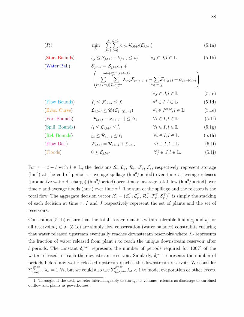
88

(Pt) minX

J∑j=1

L−1∑l=0

κjt+lKjt+l(Ej,t+l) (5.1a)

(Stor. Bounds) sj ≤ Sj,t+l − Ej,t+l ≤ sj ∀j ∈ J, l ∈ L (5.1b)(Water Bal.) Sj,t+l = Sj,t+l−1 + ∑

i−∈I−(j)

minδmaxi−

,t+l−1∑l=δmin

i−

λi− lFi−,t+l−l −∑

i+∈I+(j)Fi+,t+l + αj,t+lξt+l

∀j ∈ J, l ∈ L (5.1c)

(Flow Bounds) fi≤ Fi,t+l ≤ fi ∀i ∈ I, l ∈ L (5.1d)

(Evac. Curve) Li,t+l ≤ Ci(Sj−(i),t+l) ∀i ∈ Ievac, l ∈ L (5.1e)(Var. Bounds) |Fi,t+l −Fi,t+l−1| ≤ ∆i ∀i ∈ I, l ∈ L (5.1f)(Spill. Bounds) li ≤ Li,t+l ≤ li ∀i ∈ I, l ∈ L (5.1g)(Rel. Bounds) ri ≤ Ri,t+l ≤ ri ∀i ∈ I, l ∈ L (5.1h)(Flow Def.) Fi,t+l = Ri,t+l + Li,t+l ∀i ∈ I, l ∈ L (5.1i)(Floods) 0 ≤ Ej,t+l ∀j ∈ J, l ∈ L. (5.1j)

For τ = t + l with l ∈ L, the decisions Sτ ,Lτ , Rτ , Fτ , Eτ , respectively represent storage(hm3) at the end of period τ , average spillage (hm3/period) over time τ , average releases(productive water discharge) (hm3/period) over time τ , average total flow (hm3/period) overtime τ and average floods (hm3) over time τ 1. The sum of the spillage and the releases is thetotal flow. The aggregate decision vector Xτ = (S>τ ,L>τ , R>τ ,F>τ , E>τ )> is simply the stackingof each decision at time τ . I and J respectively represent the set of plants and the set ofreservoirs.

Constraints (5.1b) ensure that the total storage remains within tolerable limits sj and sj forall reservoirs j ∈ J . (5.1c) are simply flow conservation (water balance) constraints ensuringthat water released upstream eventually reaches downstream reservoirs where λil representsthe fraction of water released from plant i to reach the unique downstream reservoir afterl periods. The constant δmaxi represents the number of periods required for 100% of thewater released to reach the downstream reservoir. Similarly, δmini represents the number ofperiods before any water released upstream reaches the downstream reservoir. We consider∑δmaxi

l=δminiλil = 1, ∀i, but we could also use∑δmaxi

l=δminiλil < 1 to model evaporation or other losses.

1. Throughout the text, we refer interchangeably to storage as volumes, releases as discharge or turbinedoutflow and plants as powerhouses.

89

At time t = 1, we have Sjt−1(ξ) = sj0 where sj0 represents the fixed known amount ofwater (in hm3) in reservoir j at the beginning of the time horizon. We use the approximationξjt = αjtξt where ξt and ξjt represent the total inflows over all reservoirs and the inflowsat a specific reservoir j at time t where αjt is the average fraction of total inflows at timet entering reservoir j. Inflows are expressed in hm3/period and namely come from naturalprecipitations, run-off and spring thaw.

Constraints (5.1d) ensure that flows are within limits fit, fit while constraints (5.1f) ensure

that the total flow deviation at a given plant i does not exceed a pre-specified threshold ∆i

from one period to the next. Constraints (5.1e) bound the maximum amount of water thatcan be unproductively spilled at plant i ∈ Ievac ⊂ I for a given storage in the upstreamreservoir, where Ievac is the set of plants with such constraints. This relationship is givenby the non-linear function C (·) called an evacuation curve. Following Gauvin et al. (2017),we approximate it by an affine function in our model, but maintain the true structure inour simulations. We successfully tested more precise representations by introducing binarydecisions, but found that our simple affine approximation has negligible impact on the finalresults.

Equations (5.1g) ensure respect of absolute upper and lower bounds. These constraints aredetermined by specific physical characteristic of given plants. Constraints (5.1h) ensure thereleases at plant i are within prescribed bounds rit, rit, ∀t. These are based on navigationand flood safety thresholds as well as agreements with riparian communities. Finally, (5.1i)defines the total flow as the sum of unproductive spillage and releases.

We explicitly model spills and releases separately for illustrative purposes and to facilitate theextension to the case where hydroelectrical generation and spills should also be optimized.However, this is not necessary for flood-minimizing purposes, and it would be possible toreduce the dimensionality of the problem by aggregating both decisions to consider onlytotal flows. In this situation, the upper bounds on total flows become a function of theupstream storage due to the evacuation curves.

Constraints (5.1j) define overflows (floods) with respect to the critical storage levels sjt, sjtand represent quantities we wish to minimize. Since the bounds are taken with respect toa given useful reservoir storage, underflows (droughts) can theoretically exist at a reservoirj, but are physically bounded by a small constant 0 < εj and are highly undesirable. Wetherefore chose to forbid them, even if they can be added to our model very straightforwardly.

We consider a convex quadratic penalization function : Kjt(Ejt) = aE2jt with a > 0 in the

objective (5.3) to reflect the fact that larger floods have increasingly disastrous consequences.It is possible to extend our formulation to more general functions such as the ones considered

90

in Pianosi and Soncini-Sessa (2009) by introducing binary decisions to model discontinuitiesand non-convexities. However, this would lead to a mixed integer program and would affectthe tractability of our model and ultimately its use by decision makers. Indeed, our model maybe solved frequently to analyse what-if scenarios and therefore needs to be rapidly solvableby commercial off-the-shelf software. Moreover, Section 5.5 shows it leads to good empiricalresults.

The parameters κj,t > 0 in (5.3) represent the relative weight of each reservoir at a given time.We define the set J crit representing reservoirs located near riparian populations and high risksof floods as well as those with critical importance. We then fix κjt = Wκ, ∀j ∈ J crit, t forsome large W ∈ N and some fixed κ > 0 and impose that the sum of the weights equal oneso that we have a convex combination. For our problem, the dichotomy between critical andnon-critical reservoirs is unequivocal, but we could easily adapt this to more intricate cases.

5.2.2 Sources of uncertainty

We focus on the stochasticity surrounding inflows which is one of the main factors of therisks of floods and droughts. We therefore study the discrete time stochastic process ξtrepresenting total inflows over the river system at time t ∈ Z where the ξt : Ω → R arereal valued random variables bounded and non-negative with probability one. Although wefocus on minimizing the risk of floods for a finite time interval T, the process ξtt∈Z extendsinfinitely far in the past and the future. We denote the mean and variance at time t ∈ Z asE [ξt] = µt and E [(ξt − µt)2] = σ2

t .

5.2.3 General framework

We consider a dynamic setting were the true realization of the random process ξt is gra-dually revealed as time unfolds over the horizon of T days (Delage and Iancu; Shapiro et al.,2009). A sequence of controls Xt must be fixed at each stage t ∈ T after observing therealized history ξ[t−1], but before knowing the future random variables. Once ξ[t−1] is known,Xt can be implemented to yield the actual decisions Xt(ξ[t−1]) ∈ Rnt where nt ∈ N representsthe number of decisions to be taken at time t. This decision process can be visualized inFigure 5.1.

91

X1 fixed ξ1 observed · · · XT ξT

0 1 · · · T − 1 TTime TTime 1

Figure 5.1 Sequential Dynamic Decision Process

5.2.4 Affine decision rules

To consider this uncertainty and formulate the stochastic version of model (5.1), we changethe decision variables X to functions X (·) of the underlying stochastic process. We specificallyconsider simple affine functions of the uncertain inflows, which are a restricted class of possiblysuboptimal policies. These decision rules were popularized in dynamic/adjustable robustoptimization models by Ben-Tal et al. (2004) and have gained considerable attention in therecent years, namely in the field of energy (Gauvin et al., 2017; Apparigliato, 2008; Lorca andSun, 2015; Rocha and Kuhn, 2012). Although they do not guarantee optimality in general,they often lead to good-quality solutions that can be obtained very efficiently.

At the beginning of period t ∈ T, we let Kτ = nτ−1 + 1, · · · , nτ−1 + nτ represent theindices associated with decisions at time τ = t + l for lead times l ∈ L and horizon L ∈0, · · · , T−t+1. We can then express affine functions of the future inflow vector ξ ≡ ξ[t,t+L−1]

in the form :

Xk,t+l(ξ) = X 0k,t+l +

L−1∑l′=0X l′

k,t+lξt+l′ , (5.2)

where X l′k,t+l ∈ R for k ∈ Kt+l, t ∈ T and l, l′ ∈ L. The decisions pertaining to spillage,

flow and discharge represent real implementable decisions used by river operators to controlthe dynamics of the river system. Decisions that must be implemented at some future timeτ = t+ l for l ∈ L can therefore only depend on information up to time τ − 1. We thereforerequire that : X l′

k,t+l = 0, ∀l′ ≥ l and k ∈ Kimplt+l ⊂ Kt+l where the Kimpl

t+l represents the set ofindices associated to such decisions at time t+ l.

However, storage and flood are analysis variables that are only meant to track the evolutionof the system. As such, decisions at time τ can also depend of information up to time τ andwe enforce X l′

k,t+l = 0, ∀l′ ≥ l+ 1 and k ∈ Kt+l \Kimplt+l . In both cases, the impact of the past

observed ξ[t−1] is reflected implicitly in X 0k,t+l.

92

The stochastic lookahead model (5.1) based on affine decision rules provides the importantadvantage of avoiding the curse of dimensionality as well as the discretization of the randomvariables and decisions required to solve the problem through its dynamic programmingrecursions. This observation is important since finding a feasible solution to the deterministicmulti-stage problem (5.1b) - (5.1j) at time t requires considering minδmaxi− , t− 1 past waterreleases for all i− ∈ I−(j) and all j ∈ J as well as |J | initial storages. For the values |J | = 5and∑j∈J

∑i−∈I−(j)(δmaxi− −δmini− ) = 13 used in our case study, this leads to a state of dimension

18, which is already extremely demanding for classical dynamic programming. Consideringthe uncertainty and persistence of inflows further increases the state dimension. For instance,an autoregressive model of order p ∈ N would require an additional p states.

Moreover, it becomes much easier to consider constraints such as (5.1c) and (5.1f) that involvedecisions in multiple periods. Finally, Section 5.3.7 shows that by leveraging techniques fromrobust optimization, we are able to formulate each lookahead problem as a tractable convexprogram that can be solved in a single "forward" phase and that makes limited distributionassumptions compared with SDP or stochastic programming based on scenario trees.

5.2.5 Minimizing flood risk

We define the risk of floods at the beginning of time t as the conditional expected value ofthe penalized aggregated flood ∑J

j=1∑L−1l=0 κjt+lKjt+l(Ej,t+l(ξ)) over the L period look-ahead

horizon given the information up to time t− 1 where ξ ≡ ξ[t,t+L−1]. We therefore modify theobjective (5.1a) to :

(SPt) minX (·)

E J∑j=1

L−1∑l=0

κjt+lKjt+l(Ej,t+l(ξ))|Ft−1

. (5.3)

The conditional expectation offers the advantage of being the simplest consistent and co-herent dynamic risk measure (Riedel, 2004). It also enjoys various interesting properties suchas linearity and has been extensively studied in stochastic processes as well as reservoirmanagement applications. We refer to the stochastic version of problem (5.1) at time t asSPt.

93

5.3 Exploiting time series models and linear decision rules

5.3.1 General inflow representation

The quality of the solutions returned by solving the lookahead problem SPt crucially dependson the representation of the underlying stochastic process ξt. Assuming simple independenttime series will likely lead to poor quality solutions in the presence of significant serial cor-relation. However, we also want to maintain the tractability of the overall linear programconsidering affine decision rules.

In order to achieve these conflicting objectives, we assume that at the beginning of eachtime t ∈ T, the future inflows ξ ≡ ξ[t,t+L−1] over the next L days lie within the set Ξt withprobability a.s.. We also assume that this random vector can be represented as an affinefunction of some vector % ≡ %[t,t+L−1] of real valued, uncorrelated, zero mean, second orderstationary random variables. This affine representation will allow us to construct the serialdependence empirically observed in the ξ[t,t+L−1] while exploiting the convenient statisticalproperties of the %[t,t+L−1].

For modeling and tractability purposes, we will also assume that the support of the %[t,t+L−1]

is a bounded polyhedron in RL. More specifically, we assume that there exists Ut, Vt ∈RL×L,Wt ∈ Rc×L and ut, vt ∈ RL, wt ∈ Rc for some c ∈ N such that the following represen-tation, which shares important similarities with the one presented in Lorca and Sun (2015),holds :

Ξt =

ξ ∈ RL

∣∣∣∣∣∣∣∣∣∣∣∣∣

∃ζ, % ∈ RL

ξ = Utζ + ut

ζ = Vt%+ vt

Wt% ≤ wt

(5.4a)(5.4b)(5.4c)(5.4d)

We assume that for any ξ, there exists %, ζ such that the representation (5.4) holds. Althoughthis is not required in general, we naturally assume for the rest of the paper that the %, ζ areunique. This is enforced by requiring that both Ut and Vt be of full rank L. Although thiscondition may seem strong, we will see that it arises automatically in important contexts.As detailed in Section (5.3.7), a possible advantage of this unicity is the possibility to definea correspondence between affine functions of ξ and affine functions of the uncorrelated %.

We will further assume that both Ut and Vt, as well as their inverse U−1t , V −1

t when theseexists, are lower triangular. This requirement is related to the concept of non-anticipativity

94

discussed previously and intuitively ensures that each ζt and ξt is only a function of the past%[t]. We assume that ζt, ξt and %t are perfectly known and observable at each time t.

As will become clear in the next Section, the relationship between ζ ≡ ζ[t,t+L−1] and % aswell as the structure of Vt and vt play a very important role in our analysis. We thereforeexplicitly consider the intermediary RL dimensional vector random ζ even if we could directlysubstitute (5.4c) into (5.4b). More specifically, we will consider the case where the ζt followwell-known autoregressive moving average (ARMA) time series models.

In this context, (5.4b) can be naturally interpreted as a way to remove a deterministictrend, seasonal component or perform other preprocessing as is commonly done in time seriesanalysis (Brockwell and Davis, 1987; Box et al., 2008). The % can then also be seen as theresiduals obtained after fitting a specific ARMAmodel to the ζ. We assume the random vector% lies within the polyhedron % ∈ RL : Wt% ≤ wt and show there exists systematic andsound probabilistic methods to construct these polyhedral sets. We begin by assuming thatthe %t are serially independent, but then generalize the approach by considering generalizedautoregressive conditional heteroscedastic (GARCH) time series models.

Finally, using the theory of ARMA and GARCH models, we will show how the representation(5.4) can be updated to more adequately reflect the random environment as we move forwardin time and new data is progressively observed.

5.3.2 Considering general ARMA models

This Section assumes some basic familiarity with linear AR(I)MA time series. For furtherdetails, we refer to the classic texts (Box et al., 2008; Brockwell and Davis, 1987). ARMAmodels are simple linear and discrete time series that filter the serial dependency and outputwhite noise. These time series model allow us to express future random variables as an affinefunction of independent random variables. Furthermore, their parsimonious representation,practical importance, successful utilization in past hydrological models for stochastic reservoiroptimization and linear structure make them as invaluable stochastic model that can beincorporated directly in our multi-stage stochastic problem. We assume that at each timet ∈ Z, the real valued ζt satisfy the equation :

φ(B)ζt = θ(B)%t, (5.5)

for some φ(B) = 1−∑pi=1 φiB

i and θ(B) = 1 +∑qi=1 θiB

i with φi, θi ∈ R for p, q ∈ N where

95

B represents the backshift operator acting on time indices such that Bpζt = ζt−p for allt, p ∈ Z (Box et al., 2008; Brockwell and Davis, 1987). We suppose the %t are independentidentically distributed zero mean and Ft-measurable random variables. In order to guaranteesecond order stationarity, we require that the process autocovariance function γ(l) = E [%t%t+l]depend only on l ∈ Z and in particular that the variance γ(0) = σ2

% be constant across time.For any ARMA process respecting equation (5.5), we can equivalently write :

ζt = ψ(B)%t, (5.6)

where φ(B)ψ(B) = θ(B) for some ψ(B) = ∑∞i=0 ψiB

i. We can therefore express ζt as aninfinite linear combination of past %ττ=t,t−1,···. We specifically consider the case where∑∞i=0 |ψi| < ∞. In this case, we say that the process ζt is stable. Since we assume the %

are bounded with probability 1, the representation (5.6) is essentially unique (Brockwell andDavis, 1987). We can relax the assumption that the original ζt are stable if (1−B)dζt = ζ ′t forsome d ∈ N such that the ζ ′t are stable. It follows that our framework also applies to ARIMAmodels of any integer integration order d ∈ N.

Example Consider the simple AR(1) model where ζt = φζt−1 + %t holds ∀t ∈ Z. In this case(1 − φB)∑∞i=0 ψiB

i = 1 if and only if ψi = φi, i ∈ Z+. It follows the process is stable if andonly if |φ| < 1. If φ = 1, then taking ζ ′t = ζt− ζt−1 implies that ζ ′t = %t,∀t ∈ Z are iid randomvariables that satisfy our assumptions.

Representation (5.6) is particularly useful when forecasting the future values of ζt given theinformation available at time t ∈ Z. For any t ∈ Z, l ∈ Z+ we have :

ζt+l =∞∑j=l

ψj%t+l−j︸ ︷︷ ︸ζt(l)

+l−1∑j=0

ψj%t+l−j︸ ︷︷ ︸ρt(l)

, (5.7)

where ζt(l) = E [ζt+l|Ft] is the forecast and ρt(l) = ζt+l − ζt(l) is the forecast error. Thisfollows by the linearity of conditional expectation together with E [%t+l|Ft] = %t+l if l ∈ Z−and E [%t+l|Ft] = E [%t+l] = 0 otherwise. For any t ∈ Z, l ∈ Z+, we observe that ρt(l) isFt+l measurable while ζt(l) is Ft measurable. For l ∈ Z−, the forecast coincides with theactual observed random variable and therefore ρt(l) = 0 while ζt(l) = ζt+l. The conditional

96

expectation E [ζt+l|Ft] is a natural choice of forecast as it represents the minimum meansquared error estimator of ζt+l given the information up to time t ∈ Z for l ∈ Z+ (Brockwelland Davis, 1987).

Example (continued) For the stable AR(1) model and any t ∈ Z, l ∈ Z+, we haveζt+l = φlζt and ρt(l) = ∑l−1

i=0 φi%t+l−i.

If we set ρt−1,L ≡ (ρt−1(1), · · · , ρt−1(L))> for any t ∈ Z, we can then express the forecasterror vector ρt−1,L as a linear function of the independent %[t,t+L−1]. More specifically, thefollowing holds for all L ∈ 1, · · · , T − t+ 1 :

ρt−1,L = Vt%[t,t+L−1], (5.8)

where Vt ≡ V ∈ RL×L is the following invertible and lower triangular square matrix, whichis constant across all t ∈ Z :

V =

1 · · · 0ψ1 1 ...... . . .

ψL−1 · · · ψ1 1

(5.9)

We then have the equality :

ζ[t,t+L−1] = ζt−1,L + ρt−1,L (5.10)= ζt−1,L + V %[t,t+L−1], (5.11)

where ζt−1,L ≡ (ζt−1(1), · · · , ζt−1(L))> corresponds to vt in the representation (5.4). Thestructure of V as well as the definition of ζt−1,L and ρt−1,L ensures that the representation isunique. Putting all these together yields a crisp representation of the inflows ξ[t,t+L−1] as anaffine function of %[t,t+L−1] whose structure depends on the past observations through ζt−1,L :

97

ξ[t,t+L−1] = Utζ[t,t+L−1] + ut (5.12)= Ut(ζt−1,L + ρt−1,L) + ut (5.13)= Ut(ζt−1,L + V %[t,t+L−1]) + ut. (5.14)

Example (continued) Consider the discrete time process ξt with mean E [ξt] = µt,∀tsuch that Ut = I, ut = µt and therefore ξt = ζt + µt holds ∀t. Also suppose that ζt followsa stable AR(1) model. For any t ∈ Z, l ∈ Z+ and L ∈ N, we can represent ξ[t,t+L−1] as :

ξt

ξt+1...

ξt+L−1

=

φζt−1

φ2ζt−1...

φLζt−1

+

1 · · · 0φ1 1 ...... . . .

φL−1 · · · φ1 1

%t

%t+1...

%t+L−1

+

µt

µt+1...

µt+L−1

. (5.15)

The affine representation (5.14) reveals that the ξ[t,t+L−1] vector is completely determined by%[t,t+L−1]. We therefore set σ(%s; s ≤ t) = Ft,∀t ∈ T which reflects the fact that observing%[t−1] at the beginning of time t ∈ Z gives us all the information necessary to apply the realimplementable policies at times 1, 2, · · · , t− 1.

5.3.3 Support of the joint distribution of the %t

Having defined the relationship between %, ζ and ξ, we now study the support hypothesis forthe % vector. For any L ∈ N, we specifically assume that the support of %[t,t+l−1], which alsocorresponds to the set % ∈ RL : Wt% ≤ wt described in (5.4), is a bounded polyhedron inRL given by the intersection of the following two polyhedrons 2 :

B∞L,ε = % ∈ RL : |%i|σ−1% ≤ (Lε)1/2, i = 1, · · · , L (5.16a)

B1L,ε = % ∈ RL :

L∑i=1|%i|σ−1

% ≤ Lε1/2. (5.16b)

2. The set B∞L,ε ∩B1L,ε is not strictly speaking a polyhedron since (5.16a)-(5.16b) involve the non-linear

absolute value function. Nonetheless, lifting this set using the commonly used decomposition %i = %+i − %

−i

98

Although limiting, the use of this polyhedron is motivated by a sound probabilistic interpre-tation. If the %t are (possibly unbounded) iid random variables with constant variance σ2

%,then for t, L ∈ N, the covariance matrix of % ≡ %[t,t+L−1] is simply the positive definite matrixΣ%,L = σ2

%IL where IL is the L×L identity matrix. Therefore, if tr denotes the (linear) traceoperator and % is a RL valued random vector, Markov’s inequality gives us :

P(%>Σ−1%,L% > Lε) ≤ E

[%>Σ−1

%,L%]

(Lε)−1 (5.17)

= tr(Σ−1%,LE

[%%>

])(Lε)−1 (5.18)

= ε−1. (5.19)

The polytope B∞L,ε ∩B1L,ε contains the ellipsoid B2

L,ε = % ∈ RL : %>Σ−1%,L% ≤ Lε (see 5.8.1

for more details). It follows that P(% ∈ B∞L,ε ∩B1L,ε) ≥ 1− ε−1 for all t, L ∈ N. Although we

could use B2L,ε as the support, preliminary tests demonstrate that it is preferable to consider

the exterior polyhedral approximation (5.16) to speed computations.

For our particular case, we consider a large ε and reasonably assume P(% ∈ B∞L,ε ∩B1L,ε) = 1.

If the %t are essentially bounded iid random variables with constant variance σ2%, then

this assumption is not restrictive, as we can always find an ε that respects this hypotheses.Since inflows can only take a finite value with P a.s., the essential boundedness assumptionis realistic.

In a robust optimization context, this polyhedral support would be referred to as an "uncer-tainty set" since it represents the set of possible values that the random variables can take.Our approach can be straightforwardly extended to more complex polytopes and it will retainpolynomial complexity if it is extended to the intersection of polytopes and second order orsemi-definite cones (Ben-Tal et al., 2009).

The polyhedron defined by (5.16a) - (5.16b) is namely influenced by the lead time L andextending far into the future intuitively leads to a larger set. We also note that if the calibratedtime series model fits the in-sample data poorly, then the estimated σ% will be large and hencethe size of the support will increase.

This distribution-free uncertainty set offers important advantages in the presence of limiteddata availability. Indeed, since it provides valid bounds for any distribution, the ellipsoid%>Σ−1

%,L% ≤ Lε and the enclosing polyhedral set we consider are rather large compared with

and |%i| = %+i + %−i with %+

i , %−i ≥ 0,∀i yields a polyhedron where each projected point lies in the original

B∞L,ε ∩B1L,ε (Ben-Tal et al., 2009).

99

similar sets derived from assuming specific distributions.

For instance, if we assume % is jointly normal, then P(%>Σ−1% ≤ Lε) = Fχ(Lε, L), whereFχ(x, k) is the cdf of a chi-square distribution with k degrees of freedom evaluated at x. Forthe values of ε, L used in our numerical study, Fχ(Lε, L) can be considerably larger than1− ε−1. For instance, taking ε = 16 and L = 7, we get : Fχ(Lε, L) ≈ 1 > 0.9375 = 1− ε−1.

This additional conservativeness proves beneficial with limited data as we do not constructoverly small and optimistic uncertainty sets. We also observe empirically that the distribution-free set captures a much larger proportion of the out-of-sample data than a similar set witha fixed distribution.

5.3.4 Support of the (conditional) joint distribution of the ξt

Building on these assumptions, it follows that the polyhedron given by (5.4) represents theconditional support of ξ[t,t+L−1] for L ∈ 1, · · · , T − t+ 1 given the past observed %[t−1]. Theset Ξt implicitly depends on past %[t−1] through vt ≡ ζt−1,L and is therefore perfectly known atthe beginning of time t. Given our past hypothesis on the support of % as well as knowledge of%[t−1], the future inflows ξ[t,t+L−1] reside within Ξt with probability 1. In robust optimizationterminology, this polytope can be seen as a dynamic uncertainty set determining the possiblerealizations of the random vector ξ[t,t+L−1] based on past observations.

5.3.5 Considering heteroscedasticity

We now relax the assumption that the %t are independent and consider the case when theresidual %t follow a GARCH(m, s) model where m, s ∈ N. GARCH processes have provenuseful for numerous applications, namely in the field of finance where the assumption ofconstant conditional variance is not always verified and large shocks tend to be followed byperiods of increased volatility (Garcia et al., 2005; Lamoureux and Lastrapes, 1990). As wediscuss in Section 5.5.4, this is also empirically observed in daily inflows. For further detailson GARCH processes, see Box et al. (2008); Bollerslev (1986).

In this case, we still assume that for any t ∈ Z, E [%t+l|Ft] = 0,∀l ∈ Z+, E [%t] = 0 andE [%2

t ] = σ2%. We also have E [%t+k%t+l|Ft−1] = E [%t+lE [%t+k|Ft+l] |Ft−1] = 0 for l < k ∈ L. In

other words, the %t are uncorrelated zero-mean random variables with constant varianceσ2a. However, they are not necessarily independent since they are linked through the following

relation for all t ∈ Z :

100

σ2t−1(1) = α0 +

m∑i=1

αi%2t−i +

s∑j=1

βjσ2t−1−j(1) , (5.20)

where σ2t (l) = E

[%2t+l|Ft

]3for l ∈ N and α0, αi, βj ≥ 0,∀i, j to ensure non-negativity of the

conditional variance. In 5.8.4, we show that under standard stationarity assumptions on the%t, the squared shocks %2

t satisfy the difference equation :

φ(B)(%2t − σ2

a

)= θ(B)νt. (5.21)

where the νt are zero mean uncorrelated random variables with νt = %2t − σ2

t−1(1). Thepolynomials are given by θ(B) = 1+∑s

j=1 θjBj and φ(B) = 1−∑maxs,m

i=1 φiBi for θi, φi ∈ R.

We can then find ψ(B) = ∑∞i=0 ψiB

i such that φ(B)ψ(B) = θ(B) and we therefore have :

%2t = σ2

% + ψ(B)νt. (5.22)

Similarly to the ARMA model, assuming ∑∞i=0 |ψi| <∞ with νt essentially bounded ensuresthat the representation is unique. Taking the conditional expectation on both sides of equation(5.22) at the beginning of time t allows us to obtain an expression for the conditional variancereminiscent of the conditional expectation described in Section 5.3.2. For l ∈ N, we specificallyhave :

σ2t (l) = σ2

% +∞∑j=l

ψjνt+l−j. (5.23)

We can then write the conditional covariance matrix as Σ%,L,t−1 = diag(σ2t−1(1), · · · , σ2

t−1(L)),where each conditional variance σ2

t (l) is a known value at time t for l ∈ 1, · · · , L. The matrixremains diagonal since the %t are uncorrelated (details are provided in 5.8.4). In Section5.3.7, we show how to obtain a better estimation of the expected flood penalties by exploitingthis information. Note that we keep the same support described in the preceding Section and

3. Although non-standard, we adopt the notation σ2t (l) to maintain the coherence with the past sections

and to highlight the similarities with the conditional expectation of ζt+l for some t ∈ Z and l ∈ Z+ given Ft,which we denoted ζt(l).

101

that only the objective changes compared to the initial ARMA model.

When the residuals follow a GARCH process, large past errors will boost σt−1(i) for alli ∈ 1, · · · , L over the look-ahead horizon. On one hand, a stochastic process that followsthe fitted time series model very closely will therefore generate small conditional and uncon-ditional variances. On the other hand, a poor time series model will not only lead to impreciseforecasts and a large unconditional σ%, but also to extremely large σt−1(i), which may make itmore difficult to find solutions without any storage violations. However considering a variableconditional variance may help adapt to inflows that deviate from the forecast.

5.3.6 Additional modelling considerations

The representation (5.4) assumes that ξt ∈ R, ∀t ∈ T, which is not physically meaningful sinceinflows must always be non-negative. We can correct this by using the affine representation(5.14). More precisely, we can impose ξ[t,t+L−1] ∈ RL

+ by requiring that with P a.s., the futurerandom vector %[t,t+L−1] reside within the following polyhedron, which is perfectly known atthe beginning of time t ∈ T :

% ∈ RL : UtV % ≥ −(Utζt−1,L + ut)

(5.24a)

The additional structure imposed by equation (5.24a) affects the independence and the un-correlation of the %τ , but this hypothesis may not be severely violated if the constraint is notbinding "very often", which is the case in our numerical experiments.

If the violation of independence seems severely violated and this negatively impacts perfor-mance, our modelling approach can still be used by ignoring (5.24a). This simply leads to amore conservative modelling of the uncertainty and may be considered an exterior polyhedraluncertain set on the "true" uncertainty set representing the support.

5.3.7 Optimizing the conditional expected flood penalties with affine decisionrules

We suppose that the inflow model (5.4) is correct and that the % are possibly heteroscedas-tic. Next, we consider our lookahead model SPt at the beginning of time t ∈ T with arbitrarydecision rules, after observing the past %[t−1] and ξ[t−1] for a horizon of L ∈ 1, · · · , T − t+ 1days and where ξ ≡ ξ[t,t+L−1] in a more condensed and abstract form :

102

minX

E[L−1∑l=0X>t+l(ξ)Gt+lXt+l(ξ)|Ft−1

](5.25a)

s.t.l∑l=0

At+l,t+lXt+l(ξ) ≥ C∆t+lξ + C0

t+l ∀l ∈ L P a.s. (5.25b)

l∑l=0

Dt+l,t+lXt+l(ξ) = E∆t+lξ + E0

t+l ∀l ∈ L P a.s., (5.25c)

for some At+l,t+l ∈ Rm≥t+l×nt+l , C∆

t+l ∈ Rm≥t+l×L, C0

t+l ∈ Rm≥t+l , D∆

t+l ∈ Rm=t+l×L, E0

t+l ∈Rm=

t+l ,Xt+l(ξ) ∈ Rnt+l , Gt+l ∈ Snt+l+ for l ∈ L, for m≥t ,m=t , nt ∈ N.

We now limit ourselves to affine decision rules and rewrite (5.2) in the more compact form :

Xt(ξ) = X 0t + X∆

t ξ, (5.26)

for ξ ≡ ξ[t,t+L−1] ∈ RL,X 0t ∈ Rnt and X∆

t ∈ Rnt×L whose structure depends on the non-anticipativity of the respective decisions. Assuming that constraint (5.24a) does not signifi-cantly affect the hypothesis that E [%t+l|Ft−1] = 0,∀l ∈ Z+ and setting % ≡ %[t,t+L−1], theobjective value (5.25a) then becomes :

E[L−1∑l=0X>t+l(ξ)Gt+lXt+l(ξ)|Ft−1

]=

L−1∑l=0

E[X 0,>t+l Gt+lX 0

t+l|Ft−1]

+L−1∑l=0

E[%>X∆,>

t+l Gt+lX∆t+l%|Ft−1

](5.27)

=L−1∑l=0X 0,>t+l Gt+lX 0

t+l +L−1∑l=0

tr(E[%%>|Ft−1

]X∆,>t+l Gt+lX∆

t+l)

(5.28)

=L−1∑l=0X 0,>t+l Gt+lX 0

t+l +L−1∑l=0

(X∆t+lΣ

1/2%,L,t−1)>Gt+l(X∆

t+lΣ1/2%,L,t−1),

(5.29)

where :

103

X 0t+l = X 0

t+l + X∆t+lut + X∆

t+lUtζt−1,L (5.30)X∆t+l = X∆

t+lUtV (5.31)Σ1/2%,L,t−1 = diag(σt−1(1), · · · , σt−1(L)), (5.32)

and we have used the following decomposition from Section 5.3.2 :

ξ[t,t+L−1] = Ut(ζt−1,L + V %[t,t+L−1]) + ut. (5.33)

In the case of homoscedasticity, (5.32) is simply replaced by its unconditional version Σ1/2%,L =

σ%IL. Using the definition of the conditional joint support of ξ[t,t+L−1] given by (5.4) , we seethat for any f : RL → R and k ∈ R, f(ξ) ≥ k,∀ξ ∈ Ξt ⇒ P(f(ξ[t,t+L−1]) ≥ k|Ft−1) = 1 withP a.s.. With (5.30)-(5.32), problem (5.25) can therefore be written as :

minX 0,X∆

L−1∑l=0X 0,>t+l Gt+lX 0

t+l +L−1∑l=0

(X∆t+lΣ

1/2%,L,t−1)>Gt+l(X∆

t+lΣ1/2%,L,t−1) (5.34a)

s.t. (l∑l=0

At+l,t+lX∆t+l − C

∆t+l)ξ ≥ −

l∑l=0

At+l,t+lX 0t+l + C0

t+l ∀l ∈ L, ∀ξ ∈ Ξt

(5.34b)

(l∑l=0

Dt+l,t+lX∆t+l − E

∆t+l)ξ = −

l∑l=0

Dt+l,t+lX 0t+l + E0

t+l ∀l ∈ L, ∀ξ ∈ Ξt.

(5.34c)

Its optimal solution represents an upper bound on (5.25a) - (5.25c) with arbitrary decisionrules because we limit ourselves to affine functions. Since Ξt is a polyhedron, we can handle theconstraints (5.34b) through robust optimization techniques and linear programming duality(Ben-Tal et al., 2009). We also reformulate (5.34c) without the ξ by exploiting the fact thatΞt is full dimensional and contains 0. The resulting feasible domain of the robust equivalent istherefore polyhedral. Since equation (5.34a) is of the convex quadratic type, the deterministicequivalent is a large (minimization) second-order cone program (SOCP), which can be solvedvery efficiently with interior point solvers. We give more details in 5.8.2 and 5.8.3.

From this derivation, we also see that the optimal value of problem (5.34a)-(5.34b) willbe an upper bound on the conditional expectation of (weighted) floods over the horizont, · · · , t+ L− 1 for any distribution of the %t provided that the true support remains within

104

the polyhedral support defined by (5.16a) - (5.16b), constraint (5.24a) does not affect thehypothesis of E [%t+l|Ft−1] = 0,∀l ∈ Z+ and the structure of the ARMA and GARCH modelsare correct.

As can be seen from (5.30) - (5.31) and (5.32), given X 0t+l, X∆

t+l that solve problem (5.34),it is straightforward to obtain an affine mapping in terms of the ξ when Ut and V areinvertible. Indeed, we only need to compute X∆

t+lV−1U−1

t and then subtract the constantX∆t+lut + X∆

t+lUtζt−1,L from X 0t+l. This might be beneficial if river operators prefer to have

decisions expressed directly in terms of the inflows rather than the residuals %.

5.4 Monte Carlo simulation and rolling horizon framework

Solving the stochastic version of problem (5.1a)-(5.1j) with affine decision rules at the begin-ning of time 1 for L = T provides an upper bound on the value of the "true" problem overthe horizon T when various hypotheses on %t and ξt are verified. However, simulating thebehaviour of the system with a given distribution can give a better assessment of the realperformance of these decisions. Using random variables that violate the support assumptionsalso provides interesting robustness tests.

Furthermore, the full potential of ARMA and GARCHmodels crucially depends on the abilityto assimilate new data as it is progressively revealed. Using time series model to construct asingle forecast at time 1 for the entire horizon may lead to more realistic uncertainty modellingthan considering an uncertainty set that completely ignores the serial correlation. However,computing new forecasts as inflows are progressively revealed will increase the precision ofour model. We capture this fact by considering a rolling horizon framework.

A rolling horizon framework also reflects the true behaviour of river operators who must takedecisions now at the beginning of time t for each future time t, · · · , t+ L− 1 by consideringsome horizon L ∈ N 4and will update the parameters of the model as the time horizonprogresses and new information on inflows and other random variables is revealed. Section5.5.3 also illustrates that the consequences of bad forecasts can be mitigated by adaptingpast previsions.

The rolling horizon simulation works as follows. We simulate a T dimensional trajectoryof zero-mean, constant unconditional variance and uncorrelated random variables %s[T ] ≡(%s,1, · · · , %s,T )> which together with the fixed and deterministic initial inflows ξ0

5completelydetermine inflows ξs[T ] ≡ (ξs,1, · · · , ξs,T )>. For a given scenario s at the beginning of time t,

4. We consider a rolling rather than receding horizon approach. More specifically, the future time horizonL ∈ N is held constant at each optimization and does not decrease. This reflects the true approach used byriver operators.

105

after having observed the past history ξs[t−1] and %s[t−1], the initial storage Sj,t−1(ξs[T ]) and thepast water releases Fi,t′(ξs[T ]), t′ ≤ t − 1, i ∈ I, but before knowing the future inflows ξs[t,T ],we compute the conditional expectation and variance of the inflows using the ARMA andGARCH models.

We then solve the affine problem at time t by considering the (future) time horizon t, · · · , t+L− 1 and by taking the deterministic equivalent when considering affine decision rules withthe conditional support Ξt. We then implement the first period decisions, observe the totalrandom inflow ξs,t during time t, compute the linear combination of actual floods, updateSjt(ξs[T ]) and the past water releases Ft′,i(ξs[T ]), t′ ≤ t; i ∈ I and solve SPt+1. We repeat thisstep for times t = 1, · · · , T − L+ 1 for each of S sample trajectories.

5.5 Case study

5.5.1 The river system

We apply our methodology to the Gatineau river in Québec. This hydro electrical complexis part of the larger Outaouais river basin and is managed by Hydro-Québec, the largest hy-droelectricity producer in Canada (Hydro-Québec, 2012). It is composed of 3 run-of-the-riverplants with relatively small productive capacity and 5 reservoirs, of which only Baskatongand Cabonga have significant capacity (see figure 5.2).

5. We fix ξ0 = E [ξ0] as the unconditional mean inflow at time 0.

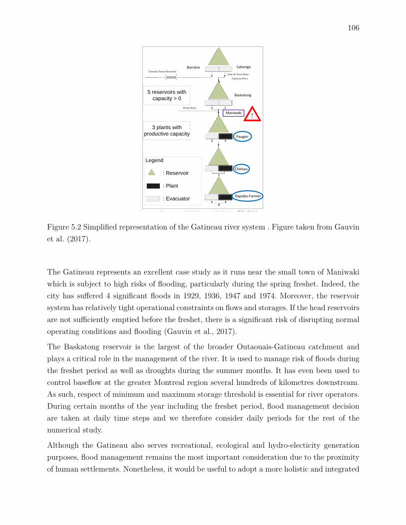
106

5 reservoirs with

capacity > 0

3 plants with

productive capacity

CabongaBarrière

Baskatong

Maniwaki

Paugan

Chelsea

Legend

: Reservoir

: Plant

: Evacuator

!

Towards Dozois Reservoir

Gatineau RiverGens e erre River

Désert River

Rapides-Farmer

Figure 5.2 Simplified representation of the Gatineau river system . Figure taken from Gauvinet al. (2017).

The Gatineau represents an excellent case study as it runs near the small town of Maniwakiwhich is subject to high risks of flooding, particularly during the spring freshet. Indeed, thecity has suffered 4 significant floods in 1929, 1936, 1947 and 1974. Moreover, the reservoirsystem has relatively tight operational constraints on flows and storages. If the head reservoirsare not sufficiently emptied before the freshet, there is a significant risk of disrupting normaloperating conditions and flooding (Gauvin et al., 2017).

The Baskatong reservoir is the largest of the broader Outaouais-Gatineau catchment andplays a critical role in the management of the river. It is used to manage risk of floods duringthe freshet period as well as droughts during the summer months. It has even been used tocontrol baseflow at the greater Montreal region several hundreds of kilometres downstream.As such, respect of minimum and maximum storage threshold is essential for river operators.During certain months of the year including the freshet period, flood management decisionare taken at daily time steps and we therefore consider daily periods for the rest of thenumerical study.

Although the Gatineau also serves recreational, ecological and hydro-electicity generationpurposes, flood management remains the most important consideration due to the proximityof human settlements. Nonetheless, it would be useful to adopt a more holistic and integrated

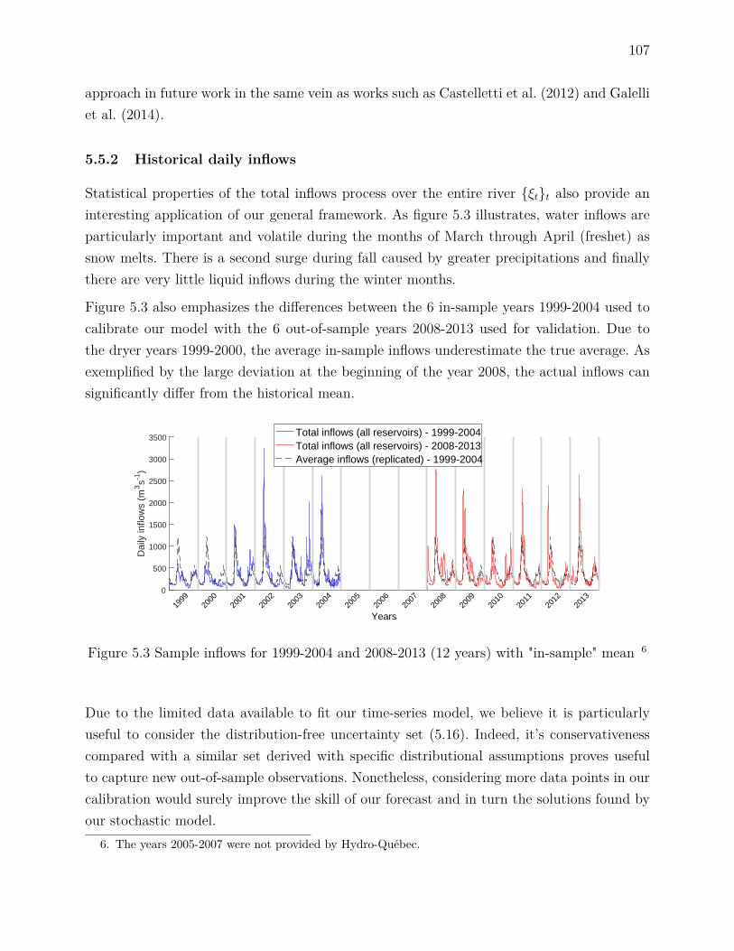
107

approach in future work in the same vein as works such as Castelletti et al. (2012) and Galelliet al. (2014).

5.5.2 Historical daily inflows

Statistical properties of the total inflows process over the entire river ξtt also provide aninteresting application of our general framework. As figure 5.3 illustrates, water inflows areparticularly important and volatile during the months of March through April (freshet) assnow melts. There is a second surge during fall caused by greater precipitations and finallythere are very little liquid inflows during the winter months.

Figure 5.3 also emphasizes the differences between the 6 in-sample years 1999-2004 used tocalibrate our model with the 6 out-of-sample years 2008-2013 used for validation. Due tothe dryer years 1999-2000, the average in-sample inflows underestimate the true average. Asexemplified by the large deviation at the beginning of the year 2008, the actual inflows cansignificantly differ from the historical mean.

0

500

1000

1500

2000

2500

3000

3500

Dai

ly in

flow

s (m

3s-1

)

1999

2000

2001

2002

2003

2004

2005

2006

2007

2008

2009

2010

2011

2012

2013

Years

Total inflows (all reservoirs) - 1999-2004Total inflows (all reservoirs) - 2008-2013Average inflows (replicated) - 1999-2004

Figure 5.3 Sample inflows for 1999-2004 and 2008-2013 (12 years) with "in-sample" mean 6

Due to the limited data available to fit our time-series model, we believe it is particularlyuseful to consider the distribution-free uncertainty set (5.16). Indeed, it’s conservativenesscompared with a similar set derived with specific distributional assumptions proves usefulto capture new out-of-sample observations. Nonetheless, considering more data points in ourcalibration would surely improve the skill of our forecast and in turn the solutions found byour stochastic model.

6. The years 2005-2007 were not provided by Hydro-Québec.

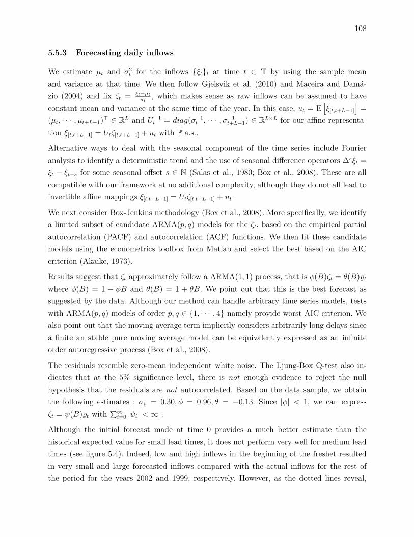
108

5.5.3 Forecasting daily inflows

We estimate µt and σ2t for the inflows ξtt at time t ∈ T by using the sample mean

and variance at that time. We then follow Gjelsvik et al. (2010) and Maceira and Damá-zio (2004) and fix ζt = ξt−µt

σt, which makes sense as raw inflows can be assumed to have

constant mean and variance at the same time of the year. In this case, ut = E[ξ[t,t+L−1]

]=

(µt, · · · , µt+L−1)> ∈ RL and U−1t = diag(σ−1

t , · · · , σ−1t+L−1) ∈ RL×L for our affine representa-

tion ξ[t,t+L−1] = Utζ[t,t+L−1] + ut with P a.s..

Alternative ways to deal with the seasonal component of the time series include Fourieranalysis to identify a deterministic trend and the use of seasonal difference operators ∆sξt =ξt − ξt−s for some seasonal offset s ∈ N (Salas et al., 1980; Box et al., 2008). These are allcompatible with our framework at no additional complexity, although they do not all lead toinvertible affine mappings ξ[t,t+L−1] = Utζ[t,t+L−1] + ut.

We next consider Box-Jenkins methodology (Box et al., 2008). More specifically, we identifya limited subset of candidate ARMA(p, q) models for the ζt, based on the empirical partialautocorrelation (PACF) and autocorrelation (ACF) functions. We then fit these candidatemodels using the econometrics toolbox from Matlab and select the best based on the AICcriterion (Akaike, 1973).

Results suggest that ζt approximately follow a ARMA(1, 1) process, that is φ(B)ζt = θ(B)%twhere φ(B) = 1 − φB and θ(B) = 1 + θB. We point out that this is the best forecast assuggested by the data. Although our method can handle arbitrary time series models, testswith ARMA(p, q) models of order p, q ∈ 1, · · · , 4 namely provide worst AIC criterion. Wealso point out that the moving average term implicitly considers arbitrarily long delays sincea finite an stable pure moving average model can be equivalently expressed as an infiniteorder autoregressive process (Box et al., 2008).

The residuals resemble zero-mean independent white noise. The Ljung-Box Q-test also in-dicates that at the 5% significance level, there is not enough evidence to reject the nullhypothesis that the residuals are not autocorrelated. Based on the data sample, we obtainthe following estimates : σ% = 0.30, φ = 0.96, θ = −0.13. Since |φ| < 1, we can expressζt = ψ(B)%t with

∑∞i=0 |ψi| <∞ .

Although the initial forecast made at time 0 provides a much better estimate than thehistorical expected value for small lead times, it does not perform very well for medium leadtimes (see figure 5.4). Indeed, low and high inflows in the beginning of the freshet resultedin very small and large forecasted inflows compared with the actual inflows for the rest ofthe period for the years 2002 and 1999, respectively. However, as the dotted lines reveal,

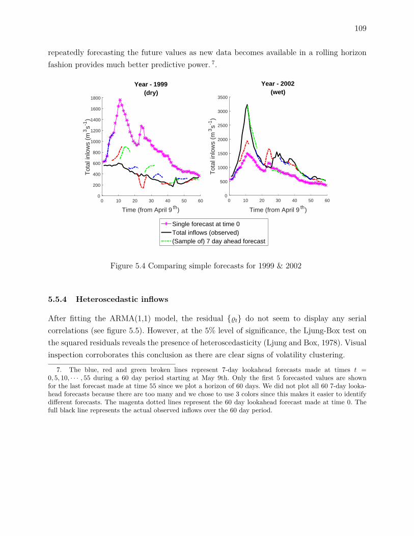
109

repeatedly forecasting the future values as new data becomes available in a rolling horizonfashion provides much better predictive power. 7.

0 10 20 30 40 50 60

Time (from April 9 th)

0

200

400

600

800

1000

1200

1400

1600

1800

Tot

al in

low

s (m

3s-1

)Year - 1999

(dry)

Single forecast at time 0Total inflows (observed)(Sample of) 7 day ahead forecast

0 10 20 30 40 50 60

Time (from April 9 th)

0

500

1000

1500

2000

2500

3000

3500

Tot

al in

low

s (m

3s-1

)

Year - 2002(wet)

Figure 5.4 Comparing simple forecasts for 1999 & 2002

5.5.4 Heteroscedastic inflows

After fitting the ARMA(1,1) model, the residual %t do not seem to display any serialcorrelations (see figure 5.5). However, at the 5% level of significance, the Ljung-Box test onthe squared residuals reveals the presence of heteroscedasticity (Ljung and Box, 1978). Visualinspection corroborates this conclusion as there are clear signs of volatility clustering.

7. The blue, red and green broken lines represent 7-day lookahead forecasts made at times t =0, 5, 10, · · · , 55 during a 60 day period starting at May 9th. Only the first 5 forecasted values are shownfor the last forecast made at time 55 since we plot a horizon of 60 days. We did not plot all 60 7-day looka-head forecasts because there are too many and we chose to use 3 colors since this makes it easier to identifydifferent forecasts. The magenta dotted lines represent the 60 day lookahead forecast made at time 0. Thefull black line represents the actual observed inflows over the 60 day period.

110

0 500 1000 1500 2000 2500−2

−1.5

−1

−0.5

0

0.5

1

1.5

2Residuals from ARMA(1,1) model

Time

Obs

erve

d re

sidu

al

Student Version of MATLAB

Figure 5.5 Residuals from ARMA(1,1) model

We find that the residual %t approximately follow a GARCH(1, 1) model with the followingestimates : α0 = 0.01, α1 = 0.14, β1 = 0.84. We can show that the coefficients in (5.23) aregiven by ψi = φi−1

1 (φ + θ) = (α1 + β1)i−1α1 since φi = (α1 + β1) and θ1 = −β1. It followsthat ∑∞i=0 |ψi| < ∞. We point out that this parsimonious GARCH process has proven veryeffective to forecast financial time-series data (Lamoureux and Lastrapes, 1990; Hansen andLunde, 2005).

5.5.5 Comparing forecasts

Sections 5.3.3 - 5.3.5 suggests that bad forecasts will lead to poor quality solutions. In or-der to evaluate the forecasting accuracy of our time series model ξfrcst,t+lL−1

l=0 , we the-refore compare it with the naive static forecast consisting of the historical daily meanξnaive,tL−1

l=0 where ξnaive,t+1 = µt+l,∀l ∈ L.. We then use the standard skill score, also knownas the Nash-Sutcliffe efficiency (Nash and Sutcliffe, 1970; Gupta et al., 2009). This statisticalmeasure can be expressed as : 1 − E [MSEfrcst,t,L]E [MSEnaive,t,L]−1 where MSEfrcst,t,L =L−1∑L−1

l=0 E[(ξfrcst,t+l − ξt+l)2

]and MSEnaive,t,L = L−1∑L−1

l=0 E [(ξt+l − µt+l)2]. A skill scoreof 1 indicates a perfect forecast with zero mean square error while a skill score of −∞ indi-cates a forecast doing infinitely worse than the reference forecast. Positive, null and negativeskill score respectively indicate superior, identical and inferior performance relative to thereference forecast.

111

5.5.6 Numerical experiments

To validate the practical importance of our multi-stage stochastic program based on ARMAand GARCH time series and affine decision rules, we perform a series of tests based ondifferent inflow generators for the Gatineau river. We consider a total horizon of T = 59 daysbeginning at the start of the spring freshet and use daily time steps. We chose this granularitybecause it corresponds to the approach used by river operators to manage the river duringthe freshet. We concentrate on the freshet as it represents the most difficult and interestingcase for our problem. However, we only report results for the first 30 days, which are alsothe most volatile and wet.

All experiments are performed by solving the problem in a rolling horizon fashion. Eachoptimization problem uses a lookahead period of L = 30 days and we perform 30 model reso-lutions for each simulated inflow trajectory. For each resolution, we only consider uncertaintyon a limited time horizon of 7 days and use the deterministic mean inflows for the remaining23 days. This reduces the impact of poor quality forecasts and speeds up computations.

To test the robustness of the different methods and evaluate if our approach could be usedto avoid emptying the head reservoirs before spring as is currently done, we always consideran initial storage that is considerably higher than the normal operating conditions for thisperiod. Results were obtained by assuming no past water releases at time 0.

We used a ε1/2 = 4 which generates relatively large supports. Simulations were run on 2000randomly generated scenarios and took several hours (> 3 hours) to complete although mostindividual problems are solved in less than 5 seconds. Problems were solved using AMPLwith solver CPLEX 12.5 on computers with 16.0 GB RAM and i7 CPU’s @ 3.4 GHz.

Unfortunately, this large ε combined with very wet or dry conditions as well as the tight flowbounds at Maniwaki can make our model infeasible. When this is the case, we allow flowbounds violations in addition to floods to get complete recourse.

For simulated inflows, we present the sample CVaRα of floods for α = 10−2n, n = 0, 1, · · · , 100over the entire time horizon of T = 30 days where for the continuous random variable X, wedefine CVaRα = E[X|X > VaRα(X)] and VaRα(X) = qX(α) = inft : P(X ≤ t) ≥ α is theα quantile for some α ∈ (0, 1) (Pflug, 2000).

As in Gauvin et al. (2017), we choose to represent the empirical CVaR rather than theempirical distributions since it allows rapid graphical comparison of the expected value (α =0) and worst case (α = 1). Moreover, as mentioned namely in Bertsimas et al. (2004), CVaRis consistent with second order stochastic dominance which is of prime concern for risk aversedecision makers.

112

To evaluate the suboptimality of our policies, we also plot the expected value of the ’wait-and-see’ solution with perfect foresight. Although very simple, Section 5.5.6 reveals that thebound can be relatively tight in some cases and therefore that our models perform well undersome scenarios.

5.5.7 Simulations with ARMA(1,1) & GARCH(1,1) generator

We first assume that the %t are zero-mean uncorrelated normal variables with unconditionalvariance σ2

%. Hence these random variables violate our assumption of boundedness made inSection 5.3.3. Choosing random variables with support defined exactly by (5.16b)-(5.16a)leads to virtually no floods.

We then suppose the true inflow process ξt is given by ξt = σtζt + µt where the ζt followan ARMA(1,1) model with parameters θ and φ. We specifically fix φ = φ and θ = θ + εθ

where φ and θ are the values used by our model through prior calibration.

Under these hypothesis, the skill of the ARMA forecast relative to the naive forecast will benon-negative if and only if −0.87 ≤ εθ ≤ 0.87. This is independent of GARCH effects. Detailsare provided in 5.8.5.

As the first 2 graphs of figure 5.6 illustrate, taking −0.87 ≤ εθ ≤ 0.87 with ARMA andGARCH models unsurprisingly leads to the greatest flood reductions while only consideringan ARMA model still improves the solution quality compared to the naive forecast. The lastgraph with εθ = −5 reveals that even with negative skill, it may pay off to consider ARMA orthe combined GARCH and ARMA models when the true process follows the same structureas those used by the model.

0 50 100

, 0 (=100,)

10-2

10-1

100

101

102

103

104

105

CV

aR, (

hm3)

Empirical CVaR violationsManiwaki river segment

03=0

Var coefficient=1

0 50 100

, 0 (=100,)

10-2

10-1

100

101

102

103

104

105

CV

aR, (

hm3)

Empirical CVaR violationsManiwaki river segment

03=0

Var coefficient=2

0 50 100

, 0 (=100,)

10-2

10-1

100

101

102

103

104

105

CV

aR, (

hm3)

Empirical CVaR violationsManiwaki river segment

03=0

Var coefficient=3

ARMA(1,1)+GARCH(1,1)ARMA(1,1)NaiveLower bound

Figure 5.6 Influence of reduced forecast skill

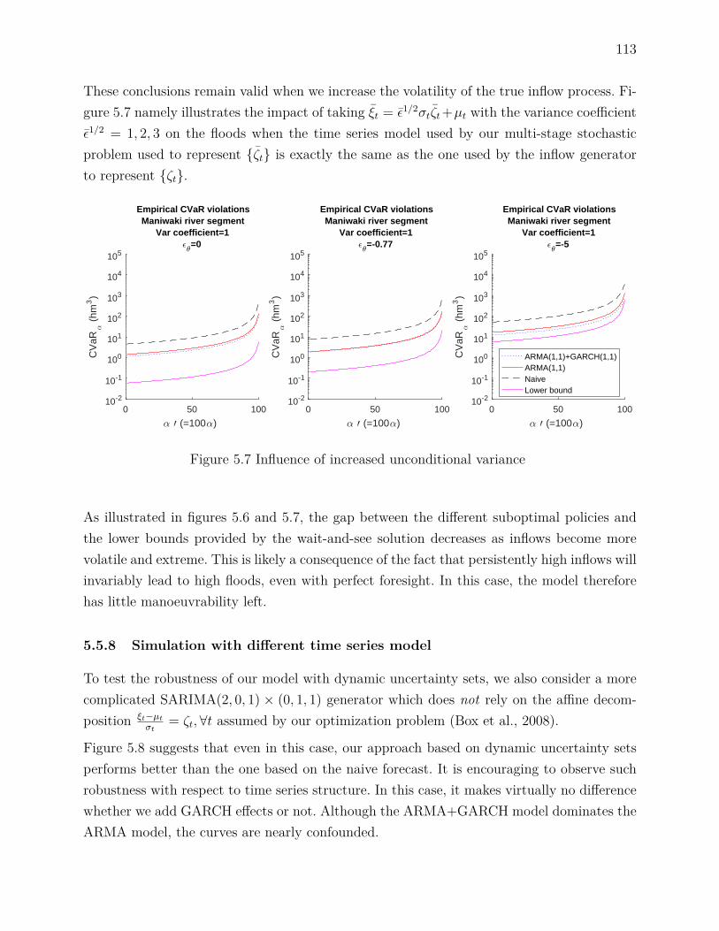
113

These conclusions remain valid when we increase the volatility of the true inflow process. Fi-gure 5.7 namely illustrates the impact of taking ξt = ε1/2σtζt+µt with the variance coefficientε1/2 = 1, 2, 3 on the floods when the time series model used by our multi-stage stochasticproblem used to represent ζt is exactly the same as the one used by the inflow generatorto represent ζt.

0 50 100

, 0 (=100,)

10-2

10-1

100

101

102

103

104

105

CV

aR, (

hm3)

Empirical CVaR violationsManiwaki river segment

Var coefficient=103=0

0 50 100

, 0 (=100,)

10-2

10-1

100

101

102

103

104

105

CV

aR, (

hm3)

Empirical CVaR violationsManiwaki river segment

Var coefficient=103=-0.77

0 50 100

, 0 (=100,)

10-2

10-1

100

101

102

103

104

105

CV

aR, (

hm3)

Empirical CVaR violationsManiwaki river segment

Var coefficient=103=-5

ARMA(1,1)+GARCH(1,1)ARMA(1,1)NaiveLower bound

Figure 5.7 Influence of increased unconditional variance

As illustrated in figures 5.6 and 5.7, the gap between the different suboptimal policies andthe lower bounds provided by the wait-and-see solution decreases as inflows become morevolatile and extreme. This is likely a consequence of the fact that persistently high inflows willinvariably lead to high floods, even with perfect foresight. In this case, the model thereforehas little manoeuvrability left.

5.5.8 Simulation with different time series model

To test the robustness of our model with dynamic uncertainty sets, we also consider a morecomplicated SARIMA(2, 0, 1) × (0, 1, 1) generator which does not rely on the affine decom-position ξt−µt

σt= ζt,∀t assumed by our optimization problem (Box et al., 2008).

Figure 5.8 suggests that even in this case, our approach based on dynamic uncertainty setsperforms better than the one based on the naive forecast. It is encouraging to observe suchrobustness with respect to time series structure. In this case, it makes virtually no differencewhether we add GARCH effects or not. Although the ARMA+GARCH model dominates theARMA model, the curves are nearly confounded.

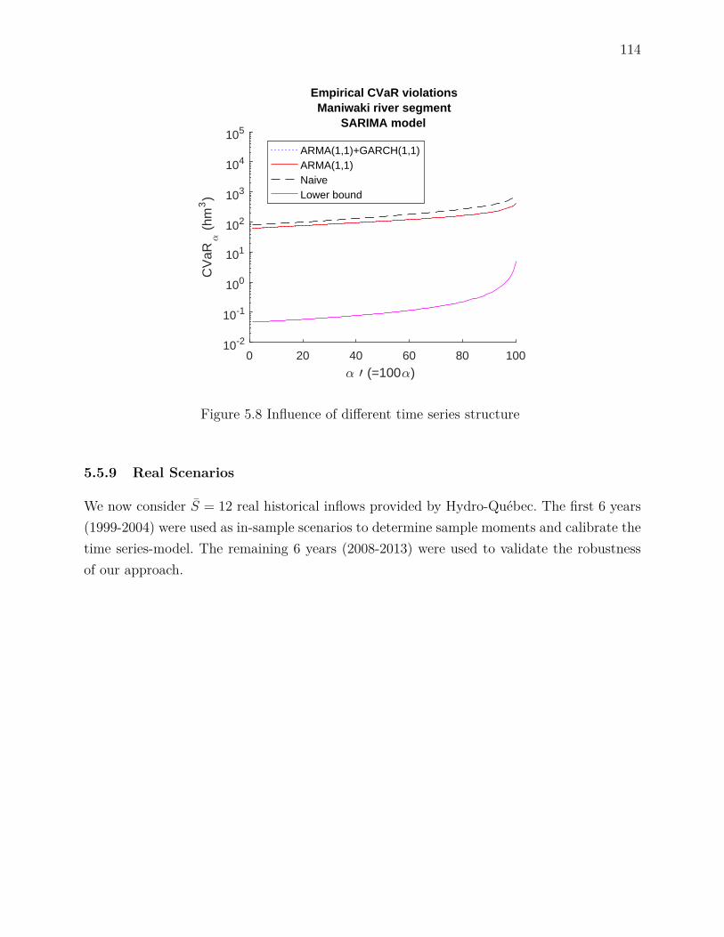
114

0 20 40 60 80 100

, 0 (=100,)

10-2

10-1

100

101

102

103

104

105

CV

aR, (

hm3)

Empirical CVaR violationsManiwaki river segment

SARIMA model

ARMA(1,1)+GARCH(1,1)ARMA(1,1)NaiveLower bound

Figure 5.8 Influence of different time series structure

5.5.9 Real Scenarios

We now consider S = 12 real historical inflows provided by Hydro-Québec. The first 6 years(1999-2004) were used as in-sample scenarios to determine sample moments and calibrate thetime series-model. The remaining 6 years (2008-2013) were used to validate the robustnessof our approach.

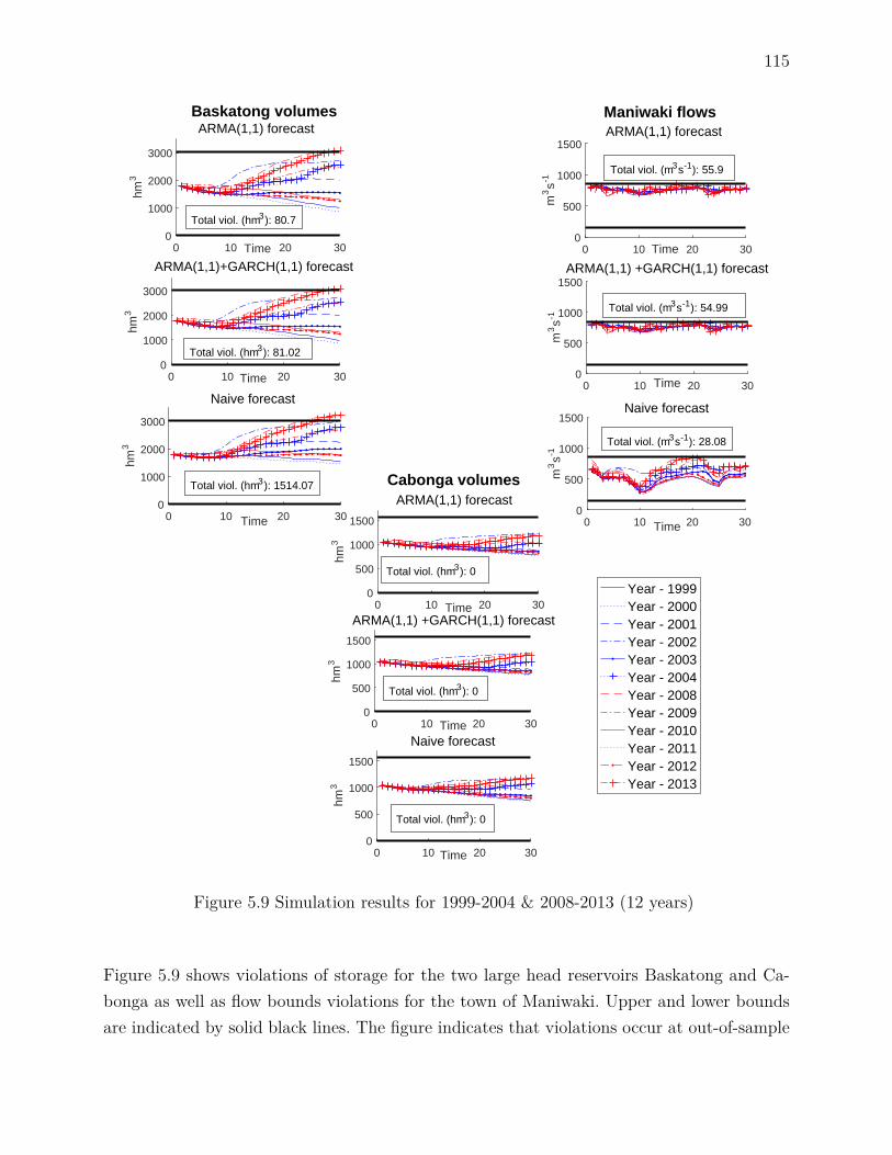
115

0 10 20 30Time0

1000

2000

3000

hm3

ARMA(1,1) forecast

0 10 20 30Time0

1000

2000

3000

hm3

ARMA(1,1)+GARCH(1,1) forecast

0 10 20 30Time0

1000

2000

3000

hm3

Naive forecast

0 10 20 30Time0

500

1000

1500

m3s-1

ARMA(1,1) forecast

0 10 20 30Time0

500

1000

1500

m3s-1

ARMA(1,1) +GARCH(1,1) forecast

0 10 20 30Time0

500

1000

1500

m3s-1

Naive forecast

0 10 20 30Time0

500

1000

1500

hm3

ARMA(1,1) forecast

0 10 20 30Time0

500

1000

1500

hm3

ARMA(1,1) +GARCH(1,1) forecast

0 10 20 30Time0

500

1000

1500

hm3

Naive forecast

Year - 1999Year - 2000Year - 2001Year - 2002Year - 2003Year - 2004Year - 2008Year - 2009Year - 2010Year - 2011Year - 2012Year - 2013

Total viol. (hm3): 80.7

Total viol. (hm3): 1514.07

Total viol. (hm3): 81.02

Total viol. (m3s-1): 54.99

Total viol. (m3s-1): 55.9

Total viol. (m3s-1): 28.08

Total viol. (hm3): 0

Total viol. (hm3): 0

Total viol. (hm3): 0

Baskatong volumes Maniwaki flows

Cabonga volumes

Figure 5.9 Simulation results for 1999-2004 & 2008-2013 (12 years)

Figure 5.9 shows violations of storage for the two large head reservoirs Baskatong and Ca-bonga as well as flow bounds violations for the town of Maniwaki. Upper and lower boundsare indicated by solid black lines. The figure indicates that violations occur at out-of-sample

116

years (in red) while in-sample years (in blue) respect all constraints. The two wet years2008 and 2013 are particularly problematic. The plots show that the models with ARMAand GARCH forecast usually yield overall superior performance compared with the naiveforecast. Indeed, these policies produce significantly less storage violations at the expenseof only slightly increased flow violations. The GARCH + ARMA and ARMA models givequalitatively similar policies.

Our results also highlight the value of parsimony and the use of criteria such as AIC thatpenalize models with numerous parameters. Complex models with higher order lags tendedto produce very bad results when tested on the out-of-sample historical inflows since theeffect of bad forecasts had lasting consequences. For instance, the abnormally high inflowsat the beginning of the freshet in 2008 resulted in residuals that were more than 10 timeshigher than the (in-sample) standard deviation at the beginning of the period. Models basedon ARMA(p,q) with large p or q produced overly wet forecasts over the next days, which ledto model infeasibility.

This issue is directly related to over-fitting problems, which have attracted considerableattention in statistics, namely in machine learning (Hastie et al., 2001). We believe that theseresults provide a counterexample to Turgeon’s claim that we should always try to optimizethe (in-sample) performance of our model and completely disregard parsimony (Turgeon,2005).

5.6 Conclusion

In conclusion, we illustrate the importance and value of considering the persistence of inflowsfor the reservoir management problem. Repeatedly solving a simple data-driven stochasticlookahead model using affine decision rules and ARMA and GARCH time series modelprovides good quality solutions for a problem that would otherwise be intractable for classicalSDP and that would require considerably more distributional assumptions for SDDP or tree-based stochastic programming.

We give detailed explanations on the construction and update of the forecasts as well as theconditional distribution of the inflows. We also generalize the approach to consider heteros-cedasticity. Although our method is applied to the reservoir management problem, variousinsights and results can be easily exported to other stochastic problems where serial correla-tion plays an important role.

As the results from Sections 5.5.7, 5.5.8 and 5.5.9 seem to suggest, it is beneficial to considerARMA and GARCH models when theses models describe the real inflow process sufficiently

117

well. When this is not the case, the stochastic models based on these forecasts may only yieldmodest benefits compared to naive static representations of the random vectors.

Nonetheless, our method offers numerous advantages that in our opinion outweigh its draw-backs. From a practical point of view, our method can be easily incorporated into an existingstochastic programming formulation based on affine decision rules. When the time seriesmodel is parsimonious, it is rather straightforward to compute the forecasts and update thestochastic model. The computational overhead is negligible and our approach can be usedfor any time series model of any structure and any order.

Combined with affine decision rules, our lookahead model is not only tractable from a theo-retical point of view, it is also extremely fast to solve. This allows us to embed our opti-mization in a heavier rolling horizon framework and to perform extensive simulations withvarious inflow generators. Although this would also be theoretically possible for other com-peting methods such as stochastic programming based on scenario trees, the computationrequirements could quickly become excessive for practical purposes (Gauvin et al., 2017).

In addition, results indicate that even when the true process differs from the model conside-red the dynamic uncertainty sets can achieve superior performance. It is likely that furtherperformance gain can be obtained by easily incorporating additional exogenous informationsuch as soil moisture at no complexity cost.

A possible avenue for further research is to extend the framework to multivariate time-series. Although this is feasible in theory, we believe it may be harder to correctly identifya multivariate model (Tsay, 2005). With limited data availability, the increased degrees offreedom provided by the multivariate model may also overfit the data and in turn producea model of questionable forecasting skill. The increased dimensionality of the problem mayalso pose numerical difficulties for multi-reservoir systems.

We also believe that it might be possible to consider ARIMA models with exogeneous va-riables such as soil moisture, temperature and weather forecasts. Although this may improvethe forecasting skill, this approach is considerably more data intensive and will make modelcalibration more difficult.

It might also be possible to combine our approach with hydrologic models by performingstatistical analysis on the forecast errors of models such as Morin and Paquet (2007) or otherensemble streamflow predictions (ESP) made by weather agencies. This might help correctthe biases of ESP forecast mentioned in Wood and Schaake (2008).

118

5.7 Acknowledgments

The authors would like to thank Charles Audet, Fabian Bastin, Angelos Georghiou, Stein-Erick Fleten and Amaury Tilmant for valuable discussion as well as everyone at Hydro-Québec and IREQ for their ongoing support, particularly Grégory Émiel, Louis Delorme,Laura Fagherazzi and Pierre-Marc Rondeau. The comments of two anonymous referee alsohelped improved the initial version of our paper. This research was supported by the NaturalSciences and Engineering Reasearch Council of Canada (NSERC) and Hydro-Québec throughthe Industrial Research Chair on the Stochastic Optimization of Electricity Generation andNSERC grant 386416-2010.

5.8 Appendix

5.8.1 Joint probabilistic guarantees for the polyhedral support

Theorem 1. For any ε > 0 and L ∈ N, we have :

|xi|σi≤√Lε, ∀i = 1, 2, · · · , L and

L∑i=1

|xi|σi≤ L√ε (5.35)

Proof 1. The matrix Σ satisfies Σ−1 = AA where A = diag(σ−11 , · · · , σ−1

L ). Classical inequa-lities between norms (see Rudin (1987) for example) ensure that :

|xi|σi≤ ‖Ax‖∞ ≤ ‖Ax‖2 , ∀i = 1, 2, · · · , L (5.36)

L∑i=1

|xi|σi

= ‖Ax‖1 ≤√L ‖Ax‖2 . (5.37)

The results follow by observing that ‖Ax‖2 =√x>Σ−1x for any x ∈ RL and justifies the use

of our bounded polyhedral support.

Observation 1. We observe that (5.35) is slightly different from the standard inclusion usedin robust optimization (Ben-Tal et al. (2009) Section 2.3 and Sim and Bertsimas (2004)).This is due to the fact that the authors in Ben-Tal et al. (2009) intersect the ellipsoid with abox (norm infinity ball) of radius 1, assume independent random variables and use Berstein’sinequality to obtain probabilistic guarantees. The authors in Sim and Bertsimas (2004) alsoderive similar uncertainty sets, but with different probabilistic guarantees because they assume

119

independent and bounded random variables with symmetric distribution.

However, the bound we derive is based on Markov’s/Chebyshev’s conditional or unconditio-nal inequality and does not require finding the maximum realisation of the random variablesexplicitly. Our bounds also hold when we weaken the requirements of independence to uncor-relation, which is required when considering heteroscedasticity and the GARCH model.

5.8.2 Equivalent reformulation of the stochastic program according to %

In order to derive the deterministic/robust equivalent of problem (5.34a)-(5.34c), it is conve-nient to formulate the problem only in terms of %. Recall the following uncertainty set forthe random inflow vector ξ :

Ξt =ξ ∈ RL

∣∣∣∣∣∣∃% ∈ ΥL,ε,t

ξ = Ut(ζt−1,L + V %) + ut

(5.38a)(5.38b)

where :

ΥL,ε,t =

% ∈ RL

∣∣∣∣∣∣∣∣∣∣∣∣

|%i|σ−1% ≤ (Lε)1/2, i = 1, · · · , L

L∑i=1|%i|σ−1

% ≤ Lε1/2

Ut(ζt−1,L + V %) + ut ≥ 0

(5.39a)

(5.39b)

(5.39c)

For any ξ ∈ Ξt, equation (5.38b) implies that the affine decision rules X (ξ) = X 0 +X∆ξ canbe written as X 0 + X∆% for some % ∈ ΥL,ε,t where :

X 0 = X 0 + X∆ut + X∆Utζt−1,L (5.40)X∆ = X∆UtV (5.41)

Since X 0 and X∆ are decision variables unrestricted in sign, we can equivalently write problem

120

(5.34a)-(5.34c) as :

minX 0,X∆

L−1∑l=0X 0,>t+l Gt+lX 0

t+l +L−1∑l=0

(X∆t+lΣ

1/2%,L,t−1)>Gt+l(X∆

t+lΣ1/2%,L,t−1) (5.42a)

s.t. (l∑l=0

At+l,t+lX∆t+l − C

∆t+l)% ≥ −

l∑l=0

At+l,t+lX 0t+l + C0

t+l ∀l ∈ L, ∀% ∈ ΥL,ε,t

(5.42b)

(l∑l=0

Dt+l,t+lX∆t+l − E

∆t+l)% = −

l∑l=0

Dt+l,t+lX 0t+l + E0

t+l ∀l ∈ L, ∀% ∈ ΥL,ε,t

(5.42c)

where C∆t+l = Ct+lUtV , C0

t+l = Ct+lUtζt−1 + Ct+lut, E∆t+l = Et+lUtV and E0

t+l =Et+lUtζt−1 + Et+lut.

5.8.3 Deriving the robust/deterministic equivalent

In order to robustify constraint (5.42b), we write ΥL,ε,t as a polyhedron in the lifted space(%+

1 , %−1 , · · · , %+

L , %−L)> ∈ R2L

+ : ∃% ∈ RL; %+i − %−i = %i; %+

i + %−i = |%i|,∀i = 1, · · · , L, whichis the image of RL under the coordinate-wise lifting Li(%) = (−min%i, 0,max%i, 0)> fori = 1, · · · , L. We specifically consider :

ΥliftL,ε |Ft−1 =

%lift =

%+1

%−1...%+L

%−L

∈ R2L

+

∣∣∣∣∣∣∣∣∣∣∣∣∣∣∣∣

Σ−1/2%,L S%lift ≤ (Lε)1/21

1>Σ−1/2%,L S%lift ≤ Lε1/2

− UtV R%lift ≤ Utζt−1,L + ut

(5.43a)(5.43b)(5.43c)

where

R =

1 −1

1 −1. . .

1 −1

∈ RL×2L

121

S =

1 1

1 1. . .

1 1

∈ RL×2L

1> = (1, · · · , 1)> ∈ RL

with S>i %lift = |%i| and R>i %lift = %i for any i = 1, · · · , L.

Robustifying the kthl ∈ 1, · · · ,mt+l constraint (5.42b) for a fixed l ∈ L can thereforebe achieved by setting α>kl(X ) = −(∑l

l=0At+l,t+lX∆t+l − C∆

t+l)>kl ∈ R1×L as the kthl row of−(∑l

l=0At+l,t+lX∆t+l − C

∆t+l) and ensuring that α>kl(X )R%lift ≤ (∑l

l=0 At+l,t+l)kl holds for all%lift ∈ Υlift

L,ε |Ft−1. Since ΥliftL,ε |Ft−1 is a closed, non-empty and bounded polyhedron, this can

be achieved by ensuring that the maximum value of the following pair of linear programs issmaller or equal than (∑l

l=0At+l,t+lX 0t+l − C

0t+l)kl :

max%lift≥0

α>kl(X )R%lift minπ,ν≥0

(Lε)1/2π>1 + π0Lε1/2 + ν>(Utζt−1,L + ut)

s. t : Σ−1/2%,L S%lift ≤ (Lε)1/21 s. t : π>Σ−1/2

%,L S + π01>Σ−1/2%,L S

(P ) 1>Σ−1/2%,L S%lift ≤ Lε1/2 (D) −ν>(UtV R) ≥ α>kl(X )R

−UtV R%lift ≤ Utζt−1,L + ut

Since ΥL,ε,t is full dimensional and contains 0, the linear system (5.42c) will hold for all% ∈ ΥL,ε,t if and only if :

−l∑l=0

Dt+l,t+lX 0t+l + E0

t+l = 0 ∈ Rnt+l (5.44a)

(l∑l=0

Dt+l,t+lX∆t+l − E

∆t+l) = 0 ∈ Rmt+l (5.44b)

122

It follows that problem (5.34a)-(5.34c) is equivalent to :

minX 0,X∆,π,ν≥0

L−1∑l=0X 0,>t+l Gt+lX 0

t+l +L−1∑l=0

(X∆t+lΣ

1/2%,L,t−1)>Gt+l(X∆

t+lΣ1/2%,L,t−1) (5.45a)

s.t. (Lε)1/2π>1 + π0Lε1/2 + ν>(Utζt−1,L + ut) ≤ (l∑l=0

At+l,t+lX 0t+l − C

0t+l)kl

∀kl ∈ 1, · · · ,ml, l ∈ L (5.45b)π>Σ−1/2

%,L S + π01>Σ−1/2%,L S − ν>(UtV R) ≥ α>kl(X )R

∀kl ∈ 1, · · · ,ml, l ∈ L (5.45c)

−l∑l=0

Dt+l,t+lX 0t+l + E0

t+l = 0 ∈ Rnt+l (5.45d)

(l∑l=0

Dt+l,t+lX∆t+l − E

∆t+l) = 0 ∈ Rmt+l (5.45e)

5.8.4 Details on GARCH(m, s) model

Recall the general GARCH(m, s) model :

σ2t−1(1) = α0 +

m∑i=1

αi%2t−i +

s∑j=1

βjσ2t−1−j(1) (5.46)

Stationarity conditions

In order for the %t to be second order stationary with constant variance σ2a we require that

for any t ∈ Z :

E[E[%2t |Ft−1

]]= E

α0 +m∑i=1

αi%2t−i +

s∑j=1

βjσ2t−1−j(1)

(5.47)

⇔ σ2% = α0

1−maxm,s∑

j=1(αj + βj)

−1

(5.48)

which is finite and positive if and only if ∑maxm,sj=1 (αj + βj) < 1 with αj = 0 if j > m and

βj = 0 if j > s.

123

Reformulation of difference equations

We can reformulate (5.46) by making the substitution νt = %2t − σ2

t−1(1) :

σ2t−1(1) = α0 +

m∑i=1

αi%2t−i +

s∑j=1

βjσ2t−1−j(1) (5.49)

⇔ %2t−i −

maxm,s∑i=1

(αi + βi)%2t−i = α0 + νt −

s∑i=1

βjνt−j (5.50)

with αi = 0 if i > m and βi = 0 if i > s. We can then rewrite (5.50) in a more compact formsimilar to the general ARMA model :

φ(B)%2t = α0 + θ(B)νt (5.51)

where φ(B) = (1 − ∑maxm,si=1 φiB

i) and θ(B) = (1 + ∑si=1 θiB

i). The coefficients of thepolynomials are given by :

φi =

1 if i = 0

(αi + βi) if i = 1, · · · ,mins,m

βi if mins,m < i ≤ maxs,m and s > m

αi if mins,m < i ≤ maxs,m and s < m

0 otherwise

and

θi =

1 if i = 0

−βi if i = 1, · · · ,m

0 otherwise.

Given conditions (5.48) :

φ(B)σ2% =

(1−∑maxm,s

j=1 (αj + βj))

(1−∑maxm,s

j=1 (αj + βj))α0 (5.52)

Hence (5.51) is equivalent to :

124

φ(B)(%2t − σ2

%) = θ(B)νt. (5.53)

Computing the conditional variance for arbitrary lead times

We can find ψ(B) such that φ(B)ψ(B) = θ(B) and we can therefore "invert" (5.53). Givenany l ∈ Z+, we specifically obtain :

%2t+l = σ2

% +∞∑i=0

ψiνt+l−i. (5.54)

Taking the conditional expectation E [·|Ft] on both sides of the equation (5.54) yields :

σ2t (l) = σ2

% +∞∑j=l

ψjνt+l−j (5.55)

Equation (5.55) holds since for j ≤ l − 1 and l ∈ Z+ :

E [νt+l−j|Ft] = E[%2t+l−j − E

[%2t+l−j|Ft+l−j−1

]|Ft

](5.56)

= E[%2t+l−j|Ft

]− E

[E[%2t+l−j|Ft+l−j−1

]|Ft

](5.57)

= 0 (5.58)

and by the linearity and towering property of the conditional expectation (Billingsley, 1995).

5.8.5 Forecast skill with synthetic ARMA(1,1) time series

If the true process follows an ARMA(1,1) model with parameters θ and φ, the quality of aL day ahead forecast made at any time t will be superior to that of the naive forecast onaverage when the skill of that forecast is non-negative :

125

0 ≤ 1− E [MSEfrcst,t,L]E [MSEnaive,t,L]−1 (5.59)

⇔L−1∑l=0

E[(σt+l(

∞∑i=0

(ψi − ψi)%t+l−i))2]≤

L−1∑l=0

E[(σt+l

∞∑i=0

ψi%t+l−i)]2

. (5.60)

If φ = φ and θ 6= θ, then (5.60) is equivalent to :

L−1∑l=0

σ2t+l

(θ − θ)2

1− φ2 σ2% ≤

L−1∑l=0

σ2t+lθ(2φ+ θ) + 1

1− φ2 σ2% (5.61)

which for values φ = −0.96 and θ = −0.13 is satisfied if and only if −1 ≤ θ ≤ 0.74. Hence ifwe have the perturbed model θ = θ+ εθ, then the skill of the forecast will be non-negative ifand only if −0.87 ≤ εθ ≤ 0.87. This is independent of GARCH effects since we consider theexpected mean square error and not the conditional expected mean square error.

126

CHAPITRE 6 ARTICLE 3: A SUCCESSIVE LINEAR PROGRAMMINGALGORITHM WITH NON-LINEAR TIME SERIES FOR THE RESERVOIR

MANAGEMENT PROBLEM

Cet article a été soumis à IEEE Transactions on Power Systems en mars 2017. Auteurs :Charles Gauvin, Erick Delage et Michel Gendreau.

Abstract : This paper proposes a multi-stage stochastic programming formulation basedon affine decision rules for the reservoir management problem. Our approach seeks to find arelease schedule that balances flood control and power generation objectives while consideringrealistic operating conditions as well as variable water head. To deal with the non-convexityintroduced by the variable water head, we implement a simple, yet effective, successive linearprogramming algorithm. We also introduce a novel non-linear inflow representation thatcaptures serial correlation of arbitrary order. We test our method on a real river system anddiscuss policy implications. Our results namely show that our method can decrease flood riskcompared to historical decisions, albeit at the cost of reduced final storages.

Keywords : Mathematical programming, Stochastic processes, Forecasting, Risk analysis

127

6.1 Nomenclature

6.1.1 Sets and parameters

T Total number of periodsL Length of look-ahead period (L ≤ T )Tt,L Look-ahead period of L periods starting at time tL Lead timesKprod. ref. Piecewise linear segments approximating the reference production curveKflood dmg. Piecewise linear segments approximating the flood damage curveKf.val. Piecewise linear segments approximating the storage value function curveI Set of plantsIevac Set of plants with evacuation curve constraintsJ Set of reservoirsj+(i), j−(i) Unique reservoir upstream or downstream of plant i, respectivelyHrefi Reference water head at plant iN refjt Reference water level at reservoir j

λil Fraction of the releases from plant i reaching the unique downstream reservoirafter l periods

δmini , δmaxi Minimum and maximum water delays for plant iκjt Relative importance of flood damages at reservoir j at time tφ Relative importance of power generation objectives compared to flood controlαjt Average proportion of the total inflows entering reservoir j at time tli, li Upper and lower bounds on total spillage at plant iri, ri Upper and lower bounds on releases at plant ifi, f i Upper and lower bounds on total releases/total flow at plant i

∆i Maximum flow variation between periods at plant isj, sj Upper and lower bounds on storage at reservoir jC ∆i , C 0

i Parameters for the linear approximation of the evacuation curve at plant ip∆ik, p

0ik Parameters for the kth segment of piecewise linear approximation of the reference

production function for plant in∆j , n

0j Parameters for the linear approximation of the water level curve for reservoir j

e∆jk, e

0jk Parameters for the kth segment of piecewise linear approximation of the flood

penalty at reservoir js∆jk, s

0jk Parameters for the kth segment of piecewise linear approximation of the final

water value function at reservoir jνt Price of 1 MWh during time tη Number of hours per period

128

6.1.2 Decision variables

Rit Releases at plant i during time tLit Spills at plant i during time tFit Total flow at plant i during time tSjt, Sjt Storage and value of storage at reservoir j at the end of time tEjt, Ejt Floods and flood damages at reservoir j at the end of time tHit Relative water head at plant i and time tPit,P totalit Reference and real production at plant i and time tNjt Water level at reservoir j and time tOfloodst Cost associated with floods at time tOprodt Cost associated with electricity generation and final value of storage at time t

6.1.3 Random variables

ξt Total inflows over all reservoirs during time tξjt Inflows at reservoir j during time tζt Logged (total) inflows during time t%t Residuals at time tFt Information known at time tΞt Dynamic uncertainty set for inflows given Ft

Ξt Exterior polyhedral approximation of Ξt

Υ Polyhedral uncertainty set for residuals

6.2 Introduction

This paper considers the optimal operation of a multi-reservoir hydro-electrical system overa given time horizon subject to uncertainty on inflows. We seek to balance hydro-electricalproduction and flood control while respecting a host of operating constraints on storages,spills, releases and water balance. Our model explicitly considers water delays as well asvariable water head. In addition, we consider inflow persistence through ARIMA time seriesof arbitrary order.

As mentioned in Labadie (2004), this stochastic multi-stage non-convex problem is extremelychallenging to solve. The variable water head and the associated non-convexity make itimpractical to find a globally optimal solution while the multi-dimensional nature of theproblem often requires various simplifications that may lead to policies of limited practicaluse (Castelletti et al., 2008).

129

To solve this problem, we propose a stochastic program based on affine decision rules, non-linear ARIMA time series and a successive linear programming (SLP) algorithm. We incorpo-rate our lightweight model in a rolling horizon framework and test it with historical inflows.Our approach builds on previous work (Gauvin et al., 2017, 2016), but makes importantimprovements in terms of modeling and empirical results, namely regarding flood reduction.

Following the work of Ben-Tal et al. (2004); Kuhn et al. (2011), affine decision rules havegained some attention for reservoir management problems and other energy-related problems(Gauvin et al., 2017; Lorca and Sun, 2015). Although they do not guarantee optimality ingeneral, these simple parametric policies often lead to good-quality solutions that can beobtained very efficiently.

Unlike competing methods such as traditional stochastic dynamic programming (SDP) (Tur-geon, 2005) and various other extensions such as sampling stochastic dynamic programming(Stedinger and Faber, 2001) and SDP based on improved discretization schemes (Zéphyret al., 2016), affine decision rules do not require discretizing the state-space, which results inimportant computational gains.

As illustrated in Gauvin et al. (2016), affine decision rules also make it possible to considerlong water delays as well as highly persistent inflows without increasing the computationalburden as would be the case of algorithms belonging to the family of SDP. Considering theselong inflow delays can be essential to avoid overly optimistic solutions in the face of floods(Gauvin et al., 2016; Turgeon, 2005; Pianosi and Soncini-Sessa, 2009).

Contrary to scenario-tree based stochastic programming and stochastic dual dynamic pro-gramming (SDDP), these decision rules also provide easily implementable policies that canbe computed off-line and used by operators for simulations.

This paper also extends Gauvin et al. (2016) and Lorca and Sun (2015) by introducing a newinflow representation based on a simple non-linear time series model. Although this leadsto a non-convex support, the resulting model has nice statistical interpretation and goodforecasting ability.

By exploiting this representation along with affine decision rules, we are able to obtain acompact bilinear expression for the objective function. In order to tackle the non-convexity,we implement a simple SLP algorithm. These algorithms have been successfully utilized inhydro-electrical reservoir management problems in the context of stochastic programs basedon scenario-trees (De Ladurantaye et al., 2009), distributionally robust optimization (Panet al., 2015) as well as at the operational level for deterministic and stochastic optimization,namely at Hydro-Québec. These experimental results suggest that this simple algorithm can

130

provide good quality solutions since the objective is bilinear and therefore well approximatedby a linear first-order Taylor approximation in a restricted neighborhood.

Considering variable water head is important since it captures the fact that a better produc-tion schedule can produce more electricity by using less water than the corresponding optimalplan with fixed head (Séguin et al., 2016a). This is also an important consideration from anoperational perspective in various regions such as Québec where cascaded river systems arewidespread. Evaluating water head is an important advantage of our method compared withSDDP since this method relies on convexity assumptions to obtain hyperplanes boundingthe optimal cost-to-go functions (Rougé and Tilmant, 2016; Pereira and Pinto, 1991; Shapiroet al., 2013).

The paper is structured as follows. We present the deterministic reservoir management pro-blem in Section 6.3. We then discuss our non-linear inflow representation and the associatednon-convex uncertainty set in Section 6.4. Section 6.5 presents the multi-stage stochasticprogram based on affine decision rules as well as the SLP algorithm used to solve it approxi-mately. We then present the river system used for our numerical experiments in Section 6.6.Section 6.7 discusses results and Section 6.8 draws concluding comments.

6.3 Deterministic formulation

6.3.1 Daily river operations

River operators must determine the average water release that will flow through the turbinesof the powerhouse i during day τ = t+ l where τ ∈ Tt,L = t, · · · , t+L− 1. For the level ofgranularity considered by our model (daily decisions), the different turbines are aggregatedand it is assumed that no maintenance occurs so that all turbines are available for powergeneration. Because of plant specificities and other physical limitations, the total releases arerequired to reside within some closed interval :

ri ≤ Riτ ≤ ri ∀i ∈ I, τ ∈ Tt,L. (6.1)

Based on physical characteristics of the sites, a certain amount of water can also be unpro-ductively spilled :

131

li ≤ Liτ ≤ li ∀i ∈ I, τ ∈ Tt,L. (6.2)

Certain sites i ∈ Ievac ⊂ I can also evacuate water through a separate spillway. Due to thephysical structure of these evacuators, the maximal amount of water that can be physicallyspilled is bounded by a function of Sjτ , the storage (hm3) in the unique upstream reservoirj−(i) at the end of time τ . We approximate these functions with affine functions parametrizedby C ∆

i ,C0i ∈ R to obtain :

Liτ ≤ C ∆i Sj−(i)τ + C 0

i , ∀i ∈ Ievac, τ ∈ Tt,L. (6.3)

We define Fiτ = Riτ + Liτ as the total flow (hm3/day) ∀i ∈ I, τ ∈ Tt,L, which is simply thesum of unproductive spillage and releases. These quantities are bounded for navigation andrecreation purposes, environmental needs as well as to ensure smooth ice formation duringthe winter months :

fi≤ Fiτ ≤ fi ∀i ∈ I, τ ∈ Tt,L. (6.4)

To avoid plant damages, we also ensure that the total flow does not change excessively fromone day to the next :

|Fiτ −Fiτ−1| ≤ ∆i ∀i ∈ I, τ ∈ Tt,L, (6.5)

where Fi,t+l are already known at time t for any l ≤ 0.

We require that the final water storage at the end of time τ at reservoir j lie within fixedbounds :

sj ≤ Sjτ ≤ sj ∀j ∈ J, τ ∈ Tt,L. (6.6)

Given very wet conditions, it is possible that the upper bound constraint (6.6) is violated.

132

We therefore introduce the non-negative variable Ejτ ≥ 0 representing floods and modify thesecond inequality to : Sjτ − Ejτ ≤ sj,∀j ∈ J, τ ∈ Tt,L. For sake of simplicity, it is assumedthat floods remain in the reservoir. Although physically possible in some cases when eithersj > 0 or reservoirs represent "useful" storages, we do not consider lower bounds violations.

We model the flood severity ($) as a piecewise linear increasing convex function of floods,which reflects the assumption that greater floods have increasing marginal consequences. Wespecifically introduce the decision variable Ejτ ≥ 0 and impose :

Ejτ ≥ e∆jkEjτ + e0

jk,∀k ∈ Kflood dmg., (6.7)

for all j, τ where Kflood dmg. = 1, · · · , Kflood dmg. and e∆jk, e

0jk define the hyperplanes. In

reality, the impact of floods are often non-convex due to threshold effects and other complexphysical phenomenon Pianosi and Soncini-Sessa (2009). However, we believe our model issatisfactory since our policies yield very limited floods when tested on historical scenarios.

Water balance constraints ensure that the current storage is given as the previous storageplus the net inflow. The net inflow is itself defined as the sum, over all upstream reservoirs,of past releases (hm3/day) weighted by the flow delay coefficients plus the daily inflows ξjt(hm3/day) during time τ less the releases from all plants during the day (hm3/day) :

Sj,τ = Sj,τ−11+

∑i−∈I−(j)

minδmaxi−

,τ−1∑l=δmin

i−

λi− lFi−,τ−l −∑

i+∈I+(j)Fi+,τ+l + ξjt, (6.8)

where Sj,t+l are already known at time t for any l ≤ 0.

for all j ∈ J, τ ∈ Tt,L where δmini− and δmaxi− represent the minimum and maximum timetaken for a drop of water released from plant i−(j) ≡ i− to reach reservoir j. We makethe simplifying assumptions that ξjt = αjtξt where αjt is the average proportion of inflowsentering reservoir j at time t and ξt are the inflows over the entire catchment at time t.

As is customarily done, we model the final water value function with a piecewise linear in-creasing concave function (Carpentier et al., 2013a). More precisely, we introduce the decisionvariable Sjτ ≥ 0 and impose :

133

Sjτ ≤ s∆jkSjτ + s0

jk,∀k ∈ Kf.val., (6.9)

for all j, τ where Kf.val. = 1, · · · , Kf.val. and s∆jk, s

0jk define the hyperplanes, which are based

on the output of other long-term scheduling tools.

The total power produced (in MW) during time τ for plant i is taken as the product of thereference production Piτ at some fixed reference water head times the relative water headHiτ (De Ladurantaye et al., 2007; Gjelsvik et al., 2010; De Ladurantaye et al., 2009) :

P totaliτ = PiτHiτ . ∀i ∈ I, τ ∈ Tt,L. (6.10)

The relative water head is given by the net water head divided by the reference water headHrefi :

Hiτ = (Nj−τ −Nj+τ )/Hrefi ∀i ∈ I, τ ∈ Tt,L. (6.11)

The net water head is simply the difference between forebayNj+τ and tailraceNj−τ elevationsduring time τ , where j+ ≡ j+(i) and j− ≡ j−(i) respectively represent the reservoir upstreamand downstream of plant i.

The forebay and tailrace elevation (m) at a given plant i are concave increasing functionsof the average storage in the upstream and downstream reservoir during time τ respectively.These functions are sufficiently well approximated by affine functions of the water storage inthe associated reservoir :

Nj−τ = n0j− + n∆

j−Sj−τ ∀j ∈ J, τ ∈ Tt,L (6.12a)Nj+τ = n0

j+ + n∆j+Sj+τ ∀j ∈ J, τ ∈ Tt,L, (6.12b)

where n0j , n

∆j ∈ R,∀j. For plants where the downstream reservoir is sufficiently far, the

tailrace water level is taken as a constant Nj− = N refj+ .

The reference production itself depends on the total flows (hm3/day). For every i and τ , we

134

use the following approximation for the reference production function by using Kprod. ref. ∈ Nhyperplanes :

Piτ ≤ p∆ikFiτ + p0

ik,∀k ∈ Kprod. ref., (6.13)

where Kprod. ref. = 1, · · · , Kprod. ref. and p∆ik, p

0ik ∈ R. Each piecewise function is increasing

only on a subset of its domain to reflect negative tailrace effects caused by excessive flows.Indeed, for each plant, we have p∆

ik > 0, k ∈ K \ Kprod. ref. and p∆iKprod. ref. < 0. Section 6.6

provides concrete examples and additional details.

6.3.2 Biobjective problem

We wish to find a production plan that balances some systemic measure of flood occurrencewhile maximizing electricity production and avoiding completely emptying the reservoirs atthe end of the horizon.

Based on previous work (Gauvin et al., 2017), we let κjt ≥ 0 reflect the relative importance offloods at reservoir j at time t where ∑j∈J κjt = 1, ∀t. We then consider Ofloodsτ , the weightedflood damages over the entire catchment at time τ ∈ Tt,L ($), which is given by the followingsimple relationship :

Ofloodsτ =∑j∈J

κjτ Ejτ . (6.14)

We evaluate the hydro-electric productive benefits associated to a reservoir release scheduleat time τ ∈ Tt,L by considering the (negative) total hydroelectric production value and thevalue of the final storage of reservoirs ($) :

Oprodτ =

−∑i∈Iprod P total,i,τ ηντ −

∑j∈J Sjτ if τ = t+ L− 1

−∑i∈Iprod P totali,τ ηντ else,(6.15)

where η is the number of hours per period, ντ is the price of 1 MWh and Sjτ indicates thefinal value of this water storage. Electricity generation is assumed constant throughout eachperiod τ . We also assume that electricity prices are known constants, which makes sense in

135

the case of Hydro-Québec.

Finally, at the beginning of time t ∈ T, we seek to minimize

t+L−1∑τ=t

((1− ϕ)Ofloodsτ + ϕOprodτ

), (6.16)

for some ϕ ∈ [0, 1] reflecting the relative importance of the aggregate production measureOprodτ compared to the aggregated flood measure Ofloodsτ .

We acknowledge that this approach has important theoretical limitations. Since we considera non-convex objective, we have no guarantee of being able to explore the set of Pareto-optimal solutions of the true problem by varying ϕ (Ehrgott, 2005). However, in practice,this simple parametrization is sufficient to gain important insights on the solution space whenconsidering simulated or historical inflows. We briefly explore these issues in Section 6.7.4.

In any case, it would be easily possible to consider a lexicographic optimization approach andminimize floods, then maximize production objectives subject to flood restrictions dependingon the optimal solution of the first problem. However, this will slightly increase computingtimes since 2 models must be successively solved.

6.4 Incorporating uncertainty

We want to model ξtt∈Z, the discrete time stochastic process representing total inflows. Ateach time t ∈ T = 1, · · · , T for the lead times L = 0, · · · , L − 1, we assume that theξ ≡ ξ[t,t+L−1] lie within the following set with probability 1 :

Ξt =

ξ ∈ RL

∣∣∣∣∣∣∣∣∣∣∣∣∣

∃ζ, % ∈ RL

ξt+l = eζt+l ,∀l ∈ L

ζ = Vt%+ vt

W% ≤ w

(6.17a)(6.17b)(6.17c)(6.17d)

where ζ ≡ ζ[t,t+L−1] and % ≡ %[t,t+L−1] represent random variables for the next future L days.We fix Vt ∈ RL×L, W ∈ Rc×L, vt ∈ RL and w ∈ Rc for some c ∈ N.

Representation (6.17) essentially states that the logarithms of inflows follow some ARIMAprocess, whose structure is codified by the matrix Vt and the vector vt, and where the residuals% are random variables taking values in the polyhedral set Υ = % ∈ RL : W% ≤ w.

136

This representation captures commonly used inflow representations as a particular case. Forinstance, considering large Υ and assuming %[t,t+L−1] follow a multivariate normal distributionimplies that the inflows are correlated and approximately follow the popular log-normaldistribution, often used in reservoir management problems (Castelletti et al., 2010; Shapiroet al., 2013; Turgeon and Charbonneau, 1998).

The exponential function used in equation (6.17b) also possesses various intuitive and sta-tistically appealing properties. Indeed, the function ensures non-negativeness of inflows andbelongs to the family of Box-Cox transforms commonly used to obtain a more adequate fitwith a theoretical model (Box and Cox, 1964).

6.5 Stochastic multi-stage formulation

We consider a dynamic setting where the inflows are progressively revealed as time unfoldsover the horizon of T days. At each time t ∈ T, the decision maker fixes a sequence of policiesto be implemented at future times τ = t, · · · , t+L−1 under the assumptions that the futureinflows ξ[t,t+L−1] belong to Ξt. Decisions must be non-anticipative in the sense that each Xτmust only be a function of the past random variables ξ[τ−1].

6.5.1 Affine decision rules

Solving the true multistage problem to optimality requires considering arbitrary functions,which will lead to an intractable problem. We therefore limit ourselves to affine policies,which are suboptimal but might still capture well the general structure of future decisions.These functions take the following form at time τ = t+ l for t ∈ T and l ∈ L :

Xkτ (ξ) = X 0kτ +

t+L−1∑τ ′=tX τ ′

kτξτ ′ . (6.18)

In this case, k ∈ nτ−1 + 1, · · · , nτ−1 + nτ and nτ ∈ N represents the number of decisionsat time τ . X 0

kτ ,X τ ′kτ ∈ R,∀k, τ become the decision variables in our deterministic equivalent

formulation. Non-anticipativity is respected by imposing X τ ′kτ = 0,∀τ ′ ≥ τ .

As mentioned in Gauvin et al. (2017) and Egging et al. (2017), we replace each decision va-riable in the deterministic formulation by its associated affine decision in the stochastic model.To ensure that the inequalities hold with probability 1, we solve an optimization problem. Forinstance, constraint (6.1) is respected with probability 1 if maxξ∈Ξt R

0it + ∑t+L−1

t′=t Rt′itξt′ ≤ r.

137

However, this optimization problem is intractable given our choice of Ξt, since this set is notgenerally convex for an arbitrary t ∈ T (see the Appendix 6.9.1). Fortunately, it is possibleto obtain the following exterior polyhedral conservative approximation :

Ξt =Ll=1

[e

minW%≤w

V >l %+vt,l, e

maxW%≤w

V >l %+vt,l]. (6.19)

Indeed, using properties of the exponential and Υ, we can check that Ξt ⊆ Ξt. The set Ξt issimply the Cartesian product of intervals (i.e. a box) and can therefore be represented withonly 2L hyperplanes.

We then use strong linear programming duality to write the deterministic equivalent as a alarge linear program (see Gauvin et al. (2017) for details).

6.5.2 Objective function and composite risk

We define the (composite) risk of the production plan at the beginning of time t as :

E[L−1∑l=0

((1− ϕ)Ofloodst+l (ξ) + ϕOprodt+l (ξ)

)|Ft−1

], (6.20)

where Ft = σ(%τ : τ ≤ t) is the σ-algebra generated by the past %τ and that we can simplyinterpret as the information known at time t (Billingsley, 1995).

By linearity of the conditional expectation, it follows that this composite risk is simply aconvex combination of the flood risk and the production risk. Appendix 6.9.2 details theanalytical expression of these terms.

6.5.3 Using successive linear programming to approximate the true problem

Due to (6.10), (6.20) contains a bilinear term (see Appendix 6.9.2 for details). In order todeal with this non-convexity, we consider a commonly used first order Taylor approximation,which is detailed in the Appendix 6.9.3, as well as a SLP algorithm (see Palacios-Gomez et al.(1982); Castillo et al. (2016) for a similar algorithm based on a first-order approximationand Nocedal and Wright (2006); Yuan (2015) for additional details on the more generalclass of trust-region algorithms). Our algorithm begins by considering the linear problem ofminimizing flood damages and builds on this solution.

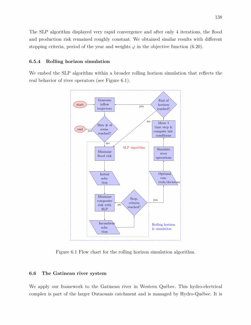
138

The SLP algorithm displayed very rapid convergence and after only 4 iterations, the floodand production risk remained roughly constant. We obtained similar results with differentstopping criteria, period of the year and weights ϕ in the objective function (6.20).

6.5.4 Rolling horizon simulation

We embed the SLP algorithm within a broader rolling horizon simulation that reflects thereal behavior of river operators (see Figure 6.1).

Generateinflow

trajectorystart

Max # ofscens.

reached?end

Minimizeflood risk

Initialsolu-tion

Minimizecompositerisk with

SLP

Incumbentsolu-tion

Stop.criteria

reached?

Optimalcon-

trols/decisions

Simulateriver

operations

Move 1time step &

compute init.conditions

End ofhorizon

reached?

no

yes

yes

no

yes

no

Rolling horizon& simulation

SLP algorithm

Figure 6.1 Flow chart for the rolling horizon simulation algorithm.

6.6 The Gatineau river system

We apply our framework to the Gatineau river in Western Québec. This hydro-electricalcomplex is part of the larger Outaouais catchment and is managed by Hydro-Québec. It is

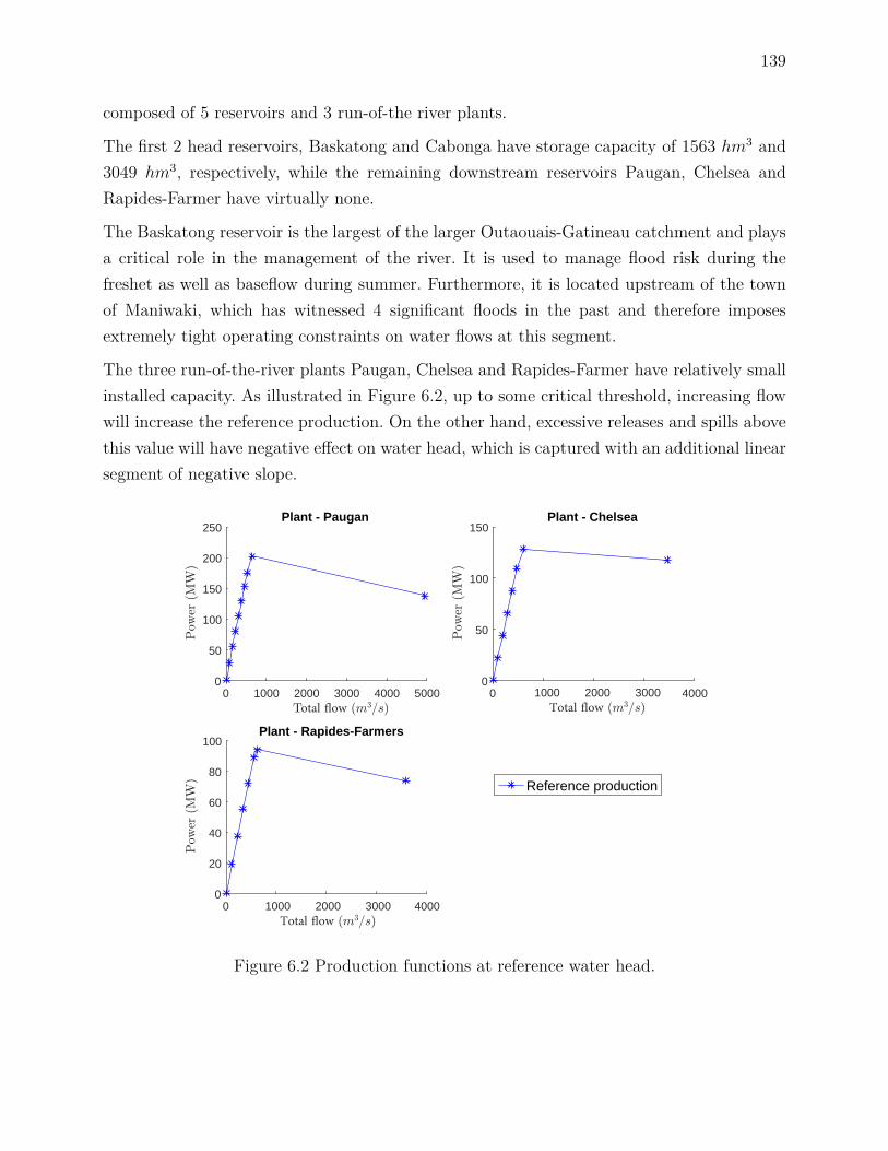
139

composed of 5 reservoirs and 3 run-of-the river plants.

The first 2 head reservoirs, Baskatong and Cabonga have storage capacity of 1563 hm3 and3049 hm3, respectively, while the remaining downstream reservoirs Paugan, Chelsea andRapides-Farmer have virtually none.

The Baskatong reservoir is the largest of the larger Outaouais-Gatineau catchment and playsa critical role in the management of the river. It is used to manage flood risk during thefreshet as well as baseflow during summer. Furthermore, it is located upstream of the townof Maniwaki, which has witnessed 4 significant floods in the past and therefore imposesextremely tight operating constraints on water flows at this segment.

The three run-of-the-river plants Paugan, Chelsea and Rapides-Farmer have relatively smallinstalled capacity. As illustrated in Figure 6.2, up to some critical threshold, increasing flowwill increase the reference production. On the other hand, excessive releases and spills abovethis value will have negative effect on water head, which is captured with an additional linearsegment of negative slope.

0 1000 2000 3000 4000 50000

50

100

150

200

250

Power

(M

W)

Plant - Paugan

0 40001000 2000 3000 Total flow (m3=s)

0

50

100

150

Power

(M

W)

Plant - Chelsea

0 40001000 2000 3000 Total flow (m3=s)

0

20

40

60

80

100

Pow

er (M

W)

Total flow (m3=s)

Plant - Rapides-Farmers

Reference production

Figure 6.2 Production functions at reference water head.

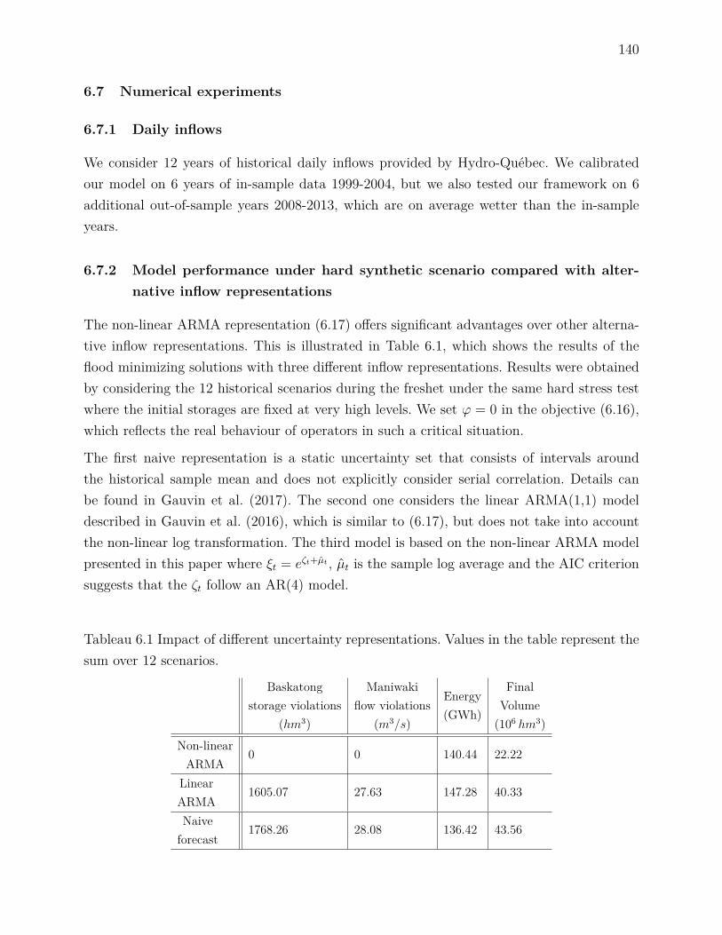
140

6.7 Numerical experiments

6.7.1 Daily inflows

We consider 12 years of historical daily inflows provided by Hydro-Québec. We calibratedour model on 6 years of in-sample data 1999-2004, but we also tested our framework on 6additional out-of-sample years 2008-2013, which are on average wetter than the in-sampleyears.

6.7.2 Model performance under hard synthetic scenario compared with alter-native inflow representations

The non-linear ARMA representation (6.17) offers significant advantages over other alterna-tive inflow representations. This is illustrated in Table 6.1, which shows the results of theflood minimizing solutions with three different inflow representations. Results were obtainedby considering the 12 historical scenarios during the freshet under the same hard stress testwhere the initial storages are fixed at very high levels. We set ϕ = 0 in the objective (6.16),which reflects the real behaviour of operators in such a critical situation.

The first naive representation is a static uncertainty set that consists of intervals aroundthe historical sample mean and does not explicitly consider serial correlation. Details canbe found in Gauvin et al. (2017). The second one considers the linear ARMA(1,1) modeldescribed in Gauvin et al. (2016), which is similar to (6.17), but does not take into accountthe non-linear log transformation. The third model is based on the non-linear ARMA modelpresented in this paper where ξt = eζt+µt , µt is the sample log average and the AIC criterionsuggests that the ζt follow an AR(4) model.

Tableau 6.1 Impact of different uncertainty representations. Values in the table represent thesum over 12 scenarios.

Baskatongstorage violations

(hm3)

Maniwakiflow violations

(m3/s)

Energy(GWh)

FinalVolume(106 hm3)

Non-linearARMA

0 0 140.44 22.22

LinearARMA

1605.07 27.63 147.28 40.33

Naiveforecast

1768.26 28.08 136.42 43.56

141

The absence of violations in the case of these extremely challenging stress tests is veryencouraging. Moreover, these flood reduction objectives are achieved without sacrificing muchenergy generation compared to the best model. These results suggest that Hydro-Québeccan maintain higher storages without violating operating constraints nor social obligations.However, Table 6.1 reveals that maintaining higher storage is of questionable value as asignificant amount of water needs to be evacuated out of the system to avoid floods.

6.7.3 Model performance under realistic historical conditions compared withhistorical decisions

Flood reduction

Next, we consider the very wet historical scenario of fall 2003. Figure 6.3 illustrates thatthese meteorological conditions led to very high storages at the Baskatong and Cabongareservoirs around early November and in turn to upper flow bounds violations of 55 m3/s

at the downstream town of Maniwaki on 3 occasions during the period November 14 toDecember 13.

We consider November 14 as the starting period, which is the day the Baskatong storagereached a level very close to maximal normal operating limits. We therefore naturally fixϕ = 0 and only focus on minimizing flood risk for the catchment. We fixed the initial storagesat their historical levels and used the realized inflows over this 30 day period.

Figure 6.3 reveals that our model out-performed the historical decisions since the productionplan leads to solutions that respect all operating constraints. We are able to respect flowbounds at Maniwaki by emptying the Baskatong reservoir faster and better anticipating thevery large inflows at times 5 and 6. Our release schedule maintains approximately the samefinal storages in Baskatong as the historical decisions, which illustrates the importance ofproperly timing the decisions. However, as in section 6.7.2, a significant amount of water isreleased from Cabonga out of the system. This result suggests that under hard scenarios, itis very hard to simultaneously reduce floods and maintain the same level of storage.

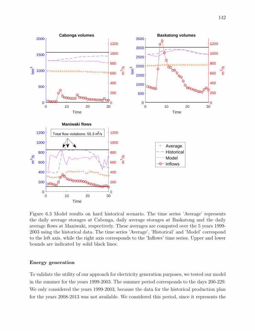
142

0 10 20 30

Time

0

500

1000

1500

2000

hm3

0

200

400

600

800

1000

1200

m3/s

Cabonga volumes

0 10 20 30

Time

0

500

1000

1500

2000

2500

3000

3500

hm3

0

200

400

600

800

1000

1200

m3/s

Baskatong volumes

0 10 20 30

Time

0

200

400

600

800

1000

1200

m3/s

0

200

400

600

800

1000

1200

m3/s

Maniwaki flows

AverageHistoricalModelInflows

Total flow violations: 55.3 m3/s

Figure 6.3 Model results on hard historical scenario. The time series ’Average’ representsthe daily average storages at Cabonga, daily average storages at Baskatong and the dailyaverage flows at Maniwaki, respectively. These averages are computed over the 5 years 1999-2003 using the historical data. The time series ’Average’, ’Historical’ and ’Model’ correspondto the left axis, while the right axis corresponds to the ’Inflows’ time series. Upper and lowerbounds are indicated by solid black lines.

Energy generation

To validate the utility of our approach for electricity generation purposes, we tested our modelin the summer for the years 1999-2003. The summer period corresponds to the days 200-229.We only considered the years 1999-2003, because the data for the historical production planfor the years 2008-2013 was not available. We considered this period, since it represents the

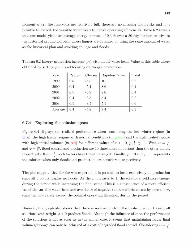
143

moment where the reservoirs are relatively full, there are no pressing flood risks and it ispossible to exploit the variable water head to derive operating efficiencies. Table 6.2 revealsthat our model yields an average energy increase of 0.3 % over a 30 day horizon relative tothe historical production plan. These figures are obtained by using the same amount of wateras the historical plan and avoiding spillage and floods.

Tableau 6.2 Energy generation increase (%) with model water head. Value in this table whereobtained by setting ϕ = 1 and focusing on energy production.

Year Paugan Chelsea Rapides-Farmer Total1999 0.5 -6.5 10.1 0.22000 0.4 -5.4 8.6 0.42001 0.5 -5.2 8.0 0.42002 0.4 -3.5 5.4 0.22003 0.1 -3.5 5.1 0.0Average 0.4 -4.8 7.4 0.3

6.7.4 Exploring the solution space

Figure 6.4 displays the realized performance when considering the low winter regime (inblue), the high freshet regime with normal conditions (in green) and the high freshet regimewith high initial volumes (in red) for different values of ϕ ∈ 0, 1

11 ,12 ,

1011 , 1. With ϕ = 1

11

and ϕ = 1011 , flood control and production are 10 times more important than the other factor,

respectively. If ϕ = 12 , both factors have the same weight. Finally, ϕ = 0 and ϕ = 1 represents

the solution when only floods and production are considered, respectively.

The plot suggests that for the winter period, it is possible to focus exclusively on productionsince all 5 points display no floods. As the ϕ increases to 1, the solutions yield more energyduring the period while increasing the final value. This is a consequence of a more efficientuse of the variable water head and avoidance of negative tailrace effects causes by excess flow,since the flow rarely exceed the optimal operating threshold during the period.

However, the graph also shows that there is no free lunch in the freshet period. Indeed, allsolutions with weight ϕ > 0 produce floods. Although the influence of ϕ on the performanceof the solutions is not as clear as in the winter case, it seems that maintaining larger finalvolumes/storage can only be achieved at a cost of degraded flood control. Considering ϕ = 1

11

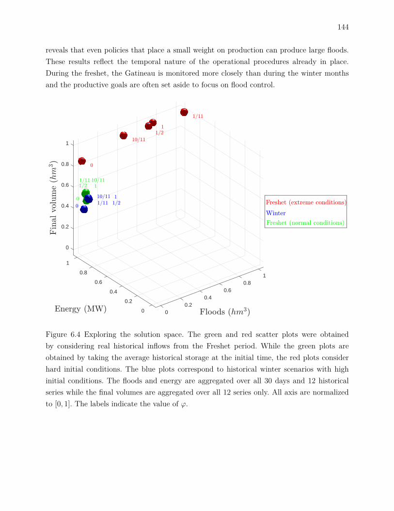
144

reveals that even policies that place a small weight on production can produce large floods.These results reflect the temporal nature of the operational procedures already in place.During the freshet, the Gatineau is monitored more closely than during the winter monthsand the productive goals are often set aside to focus on flood control.

1/2

1/11

1/11

1/2

1/21

1

0 10/11

0

10/11

0

1

0.2

1/11

0.4

0.8 1

1

Fin

alvolu

me

(hm

3)

0.6

0.6 0.8

Energy (MW)

0.8

10/11

0.6

Floods (hm3)

0.4

1

0

0.40.2

0.20 0

Freshet (normal conditions)

Winter

Freshet (extreme conditions)

Figure 6.4 Exploring the solution space. The green and red scatter plots were obtainedby considering real historical inflows from the Freshet period. While the green plots areobtained by taking the average historical storage at the initial time, the red plots considerhard initial conditions. The blue plots correspond to historical winter scenarios with highinitial conditions. The floods and energy are aggregated over all 30 days and 12 historicalseries while the final volumes are aggregated over all 12 series only. All axis are normalizedto [0, 1]. The labels indicate the value of ϕ.

145

6.8 Conclusion

This paper presents encouraging evidence that stochastic programming models based onaffine decision rules can improve short-term river management operations. Our frameworkbased on non-linear time series and a SLP algorithm can successfully consider importantphenomenon such as water delays, variable water head and inflow persistence of arbitraryorder.

More importantly, our model can yield sizable improvements when compared with historicaldecisions. We also show that it is possible to find feasible release schedules with storageconsiderably larger than average historical levels, even with high inflows. This suggests itis possible to revise the drawdown-refill cycle currently used in practice to maintain higherstorage and limit unproductive spills.

Finally, the simple convex combination of flood control and production objectives we considercan allow river operators to easily explore the solution space. It is namely interesting to assesspossible trade-offs using different inflow simulations. Since our model is extremely fast tosolve, it is highly feasible to perform such sensitivity analysis in a realistic setting.

Acknowledgment

The authors would like to thank Charles Audet, Fabian Bastin, Angelos Georghiou, GrégoryÉmiel, Louis Delorme, Pierre-Marc Rondeau, Sara Séguin and Pierre-Luc Carpentier. Thisresearch was supported by the Natural Sciences and Engineering Reasearch Council of Ca-nada (NSERC) and Hydro-Québec through the Industrial Research Chair on the StochasticOptimization of Electricity Generation and NSERC grant 386416-2010 .

6.9 Appendix

6.9.1 Details on Ξt

Time series model linking ζ and %

We assume that at each time t ∈ Z, there exists some finite constant vt such that ζt =ln ξt − vt 2 are zero mean random variables that satisfy the equation :

φ(B)ζt = θ(B)%t, (6.21)

146

where B represents the backshift operator acting on time indices such that Bpζt = ζt−p

for all t, p ∈ Z Box et al. (2008); Brockwell and Davis (1987), φ(B) = 1 − ∑pi=1 φiB

i andθ(B) = 1 +∑q

i=1 θiBi with φi, θi ∈ R for p, q ∈ N.

We also suppose %t are second order stationary zero-mean i.i.d. random variables (Boxet al., 2008) and that we can find ψ(B) = ∑∞

i=0 ψiBi where φ(B)ψ(B) = θ(B) such that∑∞

i=0 |ψi| <∞. Under suitable conditions on φ(B) and θ(B), the representation ζt = ψ(B)%tholds and is essentially unique (Brockwell and Davis, 1987).

We then exploit the following linear decomposition :

ζt(l) ≡ E [ζt+l|Ft] =l−1∑i=0

ψi%t+l−i (6.22)

ρt(l) ≡ ζt+l − ζt(l) =l−1∑i=0

ψi%t+l−i, (6.23)

for any t ∈ T and l ∈ L. ζt(l) can be naturally interpreted as a forecast of ζt+l giveninformation up to time t and ρt(l) as the forecast error.

If we set ρt−1,L ≡ (ρt−1(1), · · · , ρt−1(L))> for any t ∈ Z, we can then express the forecasterror vector ρt−1,L as a linear function of the independent %[t,t+L−1]. More specifically, ρt−1,L =Vt%[t,t+L−1] holds for all L ∈ 1, · · · , T−t+1, where Vt ≡ V ∈ RL×L is the following invertibleand lower triangular square matrix, which is constant across all t ∈ Z :

V =

1 · · · 0ψ1 1 ...... . . .

ψL−1 · · · ψ1 1

(6.24)

We then have the system of equalities :

ζ[t,t+L−1] = ζt−1,L + V %[t,t+L−1] (6.25)

2. Given S years of data where ξt,i represents the inflows on the tth period of the ith series, we can namelyconsider vt =

∑Si=1

1S ln ξt,i,∀t, the sample daily logged mean, which is also used in Shapiro et al. (2013).

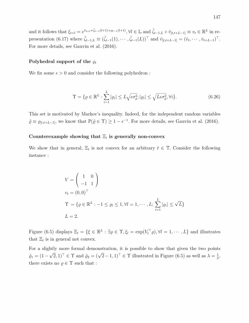
147

and it follows that ξt+l = evt+l+ζt−1(l+1)+ρt−1(l+1),∀l ∈ L and ζt−1,L + v[t,t+L−1] ≡ vt ∈ RL in re-presentation (6.17) where ζt−1,L ≡ (ζt−1(1), · · · , ζt−1(L))> and v[t,t+L−1] = (vt, · · · , vt+L−1)>.For more details, see Gauvin et al. (2016).

Polyhedral support of the %t

We fix some ε > 0 and consider the following polyhedron :

Υ = % ∈ RL :L∑i=1|%i| ≤ L

√εσ2

%; |%i| ≤√Lεσ2

%,∀i. (6.26)

This set is motivated by Markov’s inequality. Indeed, for the independent random variables% ≡ %[t,t+L−1], we know that P(% ∈ Υ) ≥ 1− ε−1. For more details, see Gauvin et al. (2016).

Counterexample showing that Ξt is generally non-convex

We show that in general, Ξt is not convex for an arbitrary t ∈ T. Consider the followinginstance :

V = 1 0−1 1

vt = (0, 0)>

Υ = % ∈ RL : −1 ≤ %l ≤ 1, ∀l = 1, · · · , L;L∑i=1|%i| ≤

√L

L = 2.

Figure (6.5) displays Ξt = ξ ∈ RL : ∃% ∈ Υ, ξl = exp(V >l %),∀l = 1, · · · , L and illustratesthat Ξt is in general not convex.

For a slightly more formal demonstration, it is possible to show that given the two points%1 = (1−

√2, 1)> ∈ Υ and %2 = (

√2− 1, 1)> ∈ Υ illustrated in Figure (6.5) as well as λ = 1

2 ,there exists no % ∈ Υ such that :

148

λ

eV>1 %1

eV>2 %1

+ (1− λ) eV

>1 %2

eV>2 %2

= eV

>1 %

eV>2 %

. (6.27)

Equivalently, we can show that ∀% ∈ Υ,

∥∥∥∥∥∥ eV

>1 %

eV>2 %

− λ eV

>1 %1

eV>2 %1

+ (1− λ) eV

>1 %2

eV>2 %2

∥∥∥∥∥∥∞

> 0.

This can be shown by solving the following linear program and observing that its optimalvalue is strictly larger than 0 :

min%+≥0,%−≥0,t≥0

t

s. t.2∑i=1

(%+i + %−i ) ≤

√2

%+i + %−i ≤ 1, ∀i = 1, 2V >i (%+ − %−)− lλi ≤ t, i = 1, 2lλi − V >i (%+ − %−) ≤ t, i = 1, 2

where lλi = ln(λeV >i %1 + (1− λ)eV >i %2) is a known constant.

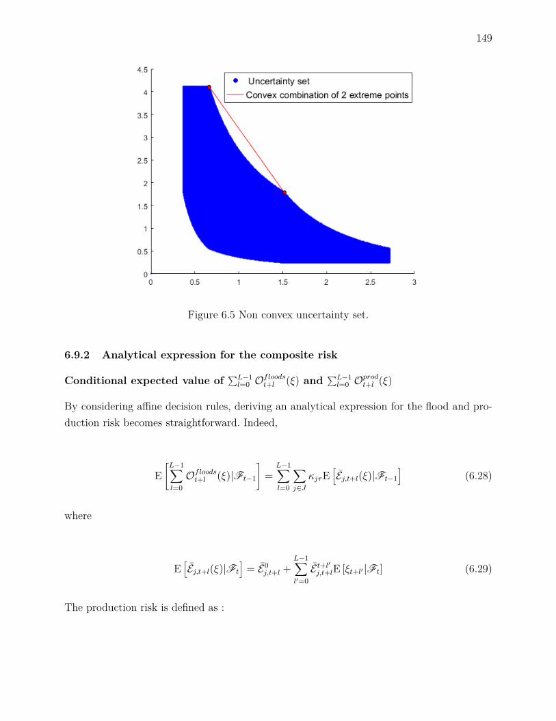
149

Figure 6.5 Non convex uncertainty set.

6.9.2 Analytical expression for the composite risk

Conditional expected value of ∑L−1l=0 O

floodst+l (ξ) and ∑L−1

l=0 Oprodt+l (ξ)

By considering affine decision rules, deriving an analytical expression for the flood and pro-duction risk becomes straightforward. Indeed,

E[L−1∑l=0Ofloodst+l (ξ)|Ft−1

]=

L−1∑l=0

∑j∈J

κjτE[Ej,t+l(ξ)|Ft−1

](6.28)

where

E[Ej,t+l(ξ)|Ft

]= E0

j,t+l +L−1∑l′=0E t+l′j,t+lE [ξt+l′ |Ft] (6.29)

The production risk is defined as :

150

E[L−1∑l=0Oprodt+l (ξ)|Ft−1

]

= −L−1∑l=0

∑i∈Iprod

E [Pi,t+l(ξ)Hi,t+l(ξ)|Ft−1]

−∑j∈J

E[Sj,t+L−1(ξ)|Ft−1

]. (6.30)

The conditional expected value of the final value of storages E[Sj,t+L−1(ξ)|Ft−1

]is defined

similarly to (6.29) while E [Pi,t+l(ξ)Hi,t+l(ξ)|Ft−1], which involves the product of two affinefunctions, is defined as :

E [Pi,t+l(ξ)Hi,t+l(ξ)|Ft−1] = P0i,t+lH0

i,t+l

+L−1∑k=0

(P0i,t+lHk

i,t+l +H0i,t+lPki,t+l)E [ξt+k|Ft−1]

+L−1∑m=0

L−1∑k=0Pmi,t+lHk

i,t+lE [ξt+mξt+k|Ft−1] . (6.31)

The conditional expectations E [ξt+k|Ft−1] and E [ξt+kξt+m|Ft−1] in (6.29) and (6.31) aredetailed in the following Section 6.9.2.

Conditional expected value of ξt+l

Theorem 2. For any t ∈ Z and l ∈ N :

E [ξt+l|Ft] = eζt(l) · E[eρt(l)

](6.32)

and for k ≥ l ≥ 1 :

E [ξt+lξt+k|Ft] = eζt(l)+ζt(k) · E[e∑k−l−1

i=0 ψi%t+k−i

]· E

[e∑k−1

i=k−l(ψi+ψl−k+i)%t+k−i]. (6.33)

151

Proof 2. This is a direct application of Theorem 34.3 of Billingsley (1995) together with theobservation that the %t are independent and hence eρt(l) = e

∑l−1i=0 ψi%t+l−i is independent of

%τtτ=−∞, which in turn implies that E[eρt(l)|Ft

]= E

[eρt(l)

].

At time t, eζt(l) is a known deterministic value for any l ∈ N that depends on the past observed%τtτ=−∞. To compute E

[e∑k

i=0 χi%t+i

]for any k ∈ 0, · · · , L and χi ∈ R, ∀i ∈ 0, · · · , L,

we perform Monte Carlo simulation.

6.9.3 First order Taylor approximation of the composite risk

We first fix E [Pi,t+l(ξ)Hi,t+l(ξ)|Ft−1] ≡ Fi,t+l(Hi,t+l,Pi,t+l) where Hi,t+l =(H0

i,t+l,Ht+1i,t+l, · · · ,Ht+L−1

i,t+l )> ∈ RL and Pi,t+l = (P0i,t+l,P t+1

i,t+l, · · · ,P t+L−1i,t+l )> ∈ RL. Gi-

ven the point (H>i,t+l, P>i,t+l)> ∈ R2L, we then obtain :

Fi,t+l(Hi,t+l,Pi,t+l)≈ Fi,t+l(Hi,t+l, Pi,t+l)

+ H0i,t+l(P0

i,t+l − P0i,t+l)

+L−1∑k=0Hki,t+l(P0

i,t+l − P0i,t+l)E [ξt+k|Ft−1]

+ P0i,t+l(H0

i,t+l − H0i,t+l)

+L−1∑k=0Pki,t+l(H0

i,t+l − H0i,t+l)E [ξt+k|Ft−1]

+L−1∑k=0P0i,t+l(Ht+k

i,t+l − Ht+ki,t+l)E [ξt+k|Ft−1]

+L−1∑m=0

L−1∑k=0P t+mi,t+l(Ht+k

i,t+l − Ht+ki,t+l)E [ξt+mξt+k|Ft−1]

+L−1∑k=0H0i,t+l(P t+ki,t+l − P t+ki,t+l)E [ξt+k|Ft−1]

+L−1∑m=0

L−1∑k=0Ht+mi,t+l(P t+ki,t+l − P t+ki,t+l)E [ξt+mξt+k|Ft−1] . (6.34)

152

CHAPITRE 7 DISCUSSION GÉNÉRALE

7.1 Synthèse des travaux

Les chapitres précédents présentent trois travaux sur la gestion mensuelle de la rivière Ga-tineau en présence d’incertitude sur les apports. Les résultats montrent que sous certainesconditions hydrologiques, il est difficile d’établir un plan de production qui respecte toujourstoutes les contraintes. Comme l’indique le chapitre 4, même en éliminant complètement l’in-certitude, il est impossible de trouver un plan de production réalisable si les niveaux d’eauet les apports sont suffisamment importants.

Comme en témoignent les résultats des chapitres 4 et 5 basés sur les règles de décision, les mo-dèles déterministes ainsi que ceux basés sur la programmation stochastique sur arbre, l’ajoutde l’incertitude complique significativement la prise de décisions et rend la minimisation desinondations très difficile. Il est donc encourageant d’obtenir une solution sans inondations auchapitre 6.

Bien que le chapitre 6 suggère que le modèle développé puisse améliorer certaines décisionshistoriques et qu’il soit possible de réduire le risque d’inondations, il semble prudent d’affirmerque le modèle ne permettra pas de révolutionner la gestion de la rivière du jour au lendemain.

Effectivement, il semble difficile, voire impossible de réduire le risque d’inondations tout enmaintenant le même stock d’eau dans tous les réservoirs. Notre modèle permet toutefoisd’explorer l’espace des solutions grâce à une expression paramétrique simple de l’objectif àoptimiser.

Cependant, les résultats des chapitres 4, 5 et 6 demeurent encourageants, car ils suggèrentque le modèle peut être utilisé efficacement et à très faibles coûts en termes de temps decalcul. L’approche par règles de décision linéaires offre assurément des avantages importantspar rapport à la prise de décision actuelle, basée sur la résolution de plusieurs modèlesdéterministes sous différents scénarios d’apports.

Le chapitre 4 suggère que l’approche par règles de décision linéaires est supérieure à cellebasée sur les arbres de scénarios au niveau des qualités fournies avec des temps de calcul si-milaires. Les règles de décision permettent également de considérer des problèmes beaucoupplus grands que ceux en programmation stochastique dynamique tout en faisant moins d’hy-pothèses sur les apports. Par ailleurs, le chapitre 6 indique que contrairement à l’algorithmeSDDP, il est possible de considérer la hauteur de chute variable avec notre méthodologie.

153

Malgré ces résultats prometteurs, plusieurs points demeurent en suspens ou sujets à amélio-ration. La section suivante fait un survol rapide des améliorations potentielles pouvant êtreétudiées lors de travaux futurs.

7.2 Limitations de la solution proposée

Les trois articles présentés aux Sections 4, 5 et 6 exploitent tous une représentation baséesur :

ξjt = αjtξt, ∀j, t (7.1)

où αjt représente la proportion moyenne des apports totaux entrant dans le réservoir j autemps t. Bien qu’elle soit compacte et réduise la dimension du problème, cette formulationsuppose implicitement que les apports sont parfaitement corrélés spatialement. Cette hypo-thèse est assez forte considérant que la distance entre certains réservoirs est importante. 1

Heureusement, la figure 7.1 suggère que l’hypothèse n’est pas complètement aberrante.

En effet, comme Baskatong reçoit systématiquement une grande proportion des apports to-taux, la représentation (7.1) a l’avantage d’expliquer une grande partie de l’incertitude. Parailleurs, comme Maniwaki se situe immédiatement en aval de Baskatong et qu’il existe uneforte corrélation entre Baskatong et Maniwaki (voir la Figure 7.2), cette représentation offreégalement l’avantage de bien prédire les apports au point névralgique de Maniwaki, ce qui serévèle utile pour éviter les inondations.

La faible corrélation entre les apports totaux et les apports aux deux derniers réservoirs n’estpas dramatique, car ces derniers reçoivent le moins d’eau de la rivière et il n’y a historiquementjamais d’inondations à ces centrales. La forme en "V" des données à ces 2 réservoirs suggèrenéanmoins la présence de deux régimes hydrologiques très différents ainsi qu’une différencestructurelle importante entre certaines années. Une analyse multivariée plus poussée semblede mise.

1. Dans la Section 1, on mentionne que la rivière Gatineau couvre une distance d’environ 400 km. Cepen-dant, il s’agit de la distance entre la source de la rivière et son exutoire non loin de la centrale Rapides-Farmer.En fait, la distance entre le barrage de Cabonga et la centrale Rapides-Farmer se situe aux alentours de 250-300 km alors que la distance entre Baskatong et Rapides-Farmer est environ de 150-200 km.

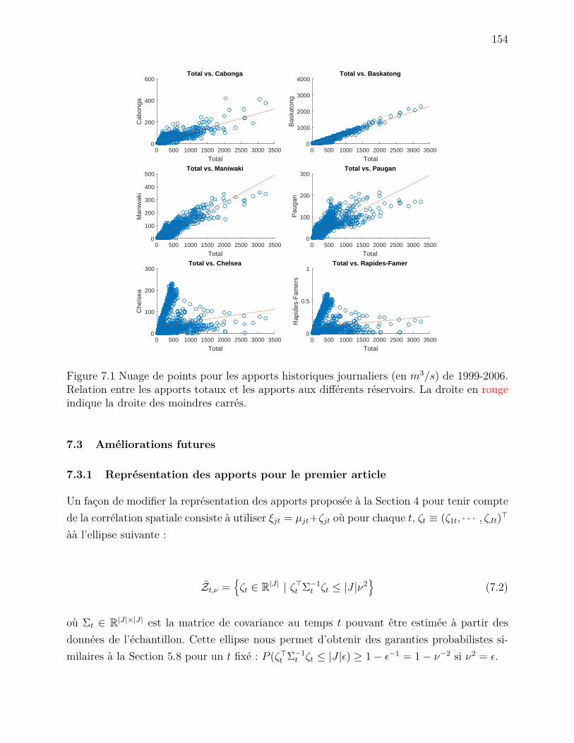
154

0 500 1000 1500 2000 2500 3000 3500

Total

0

200

400

600

Cab

onga

Total vs. Cabonga

0 500 1000 1500 2000 2500 3000 3500

Total

0

1000

2000

3000

4000

Bas

kato

ng

Total vs. Baskatong

0 500 1000 1500 2000 2500 3000 3500

Total

0

100

200

300

400

500

Man

iwak

i

Total vs. Maniwaki

0 500 1000 1500 2000 2500 3000 35000

100

200

300

Pau

gan

Total vs. Paugan

0 500 1000 1500 2000 2500 3000 3500

Total

0

100

200

300

Che

lsea

Total vs. Chelsea

0 500 1000 1500 2000 2500 3000 3500

Total

0

0.5

1

Rap

ides

-Fam

ers

Total

Total vs. Rapides-Famer

Figure 7.1 Nuage de points pour les apports historiques journaliers (en m3/s) de 1999-2006.Relation entre les apports totaux et les apports aux différents réservoirs. La droite en rougeindique la droite des moindres carrés.

7.3 Améliorations futures

7.3.1 Représentation des apports pour le premier article

Un façon de modifier la représentation des apports proposée à la Section 4 pour tenir comptede la corrélation spatiale consiste à utiliser ξjt = µjt+ζjt où pour chaque t, ζt ≡ (ζ1t, · · · , ζJt)>

àà l’ellipse suivante :

Zt,ν =ζt ∈ R|J | | ζ>t Σ−1

t ζt ≤ |J |ν2

(7.2)

où Σt ∈ R|J |×|J | est la matrice de covariance au temps t pouvant être estimée à partir desdonnées de l’échantillon. Cette ellipse nous permet d’obtenir des garanties probabilistes si-milaires à la Section 5.8 pour un t fixé : P (ζ>t Σ−1

t ζt ≤ |J |ε) ≥ 1− ε−1 = 1− ν−2 si ν2 = ε.

155

Néanmoins, on pourrait accuser cette représentation d’être "trop conservatrice", car il estpossible qu’elle contienne des déviations ζjt pouvant mener à des apports ξjt négatifs. Onpeut donc prendre l’intersection avec l’orthant non-négatif : Zt,ν ∩ ζj,t ≥ 0,∀j ∈ J quinous donne encore la garantie probabiliste 1 − ε−1, car les apports sont non-négatifs avecprobabilité 1. L’usage de cet ensemble implique que notre équivalent déterministe deviendraun second order cone problem (SOCP).

Si on choisit d’ignorer la corrélation complètement, il serait également possible d’utiliser lareprésentation polyhédrale suivante, plus près de celle utilisée dans la Section 4 : ξjt = µjt+ζjtoù pour chaque t, ζt ≡ (ζ1t, · · · , ζJt)> appartient à :

Zt,ν =ζt ∈ R|J | | −minµjt, νσjt ≤ ζjt ≤ νσjt,∀j

. (7.3)

Les σjt, µjt peuvent encore une fois être estimés à partir des données d’échantillons recueillies.

7.3.2 Représentation des apports pour le deux derniers articles

Il pourrait également être bénéfique de raffiner la représentation utilisée dans le chapitre 5.En effet, comme l’indique les Figures 7.1 et 7.2, il semble exister une corrélation spatialeplus complexe que celle supposée dans cette thèse. Afin d’avoir une meilleure compréhensiondes relations entre les apports aux différents réservoirs, une analyse par séries chronologiquesmultivariées semble prometteuse.

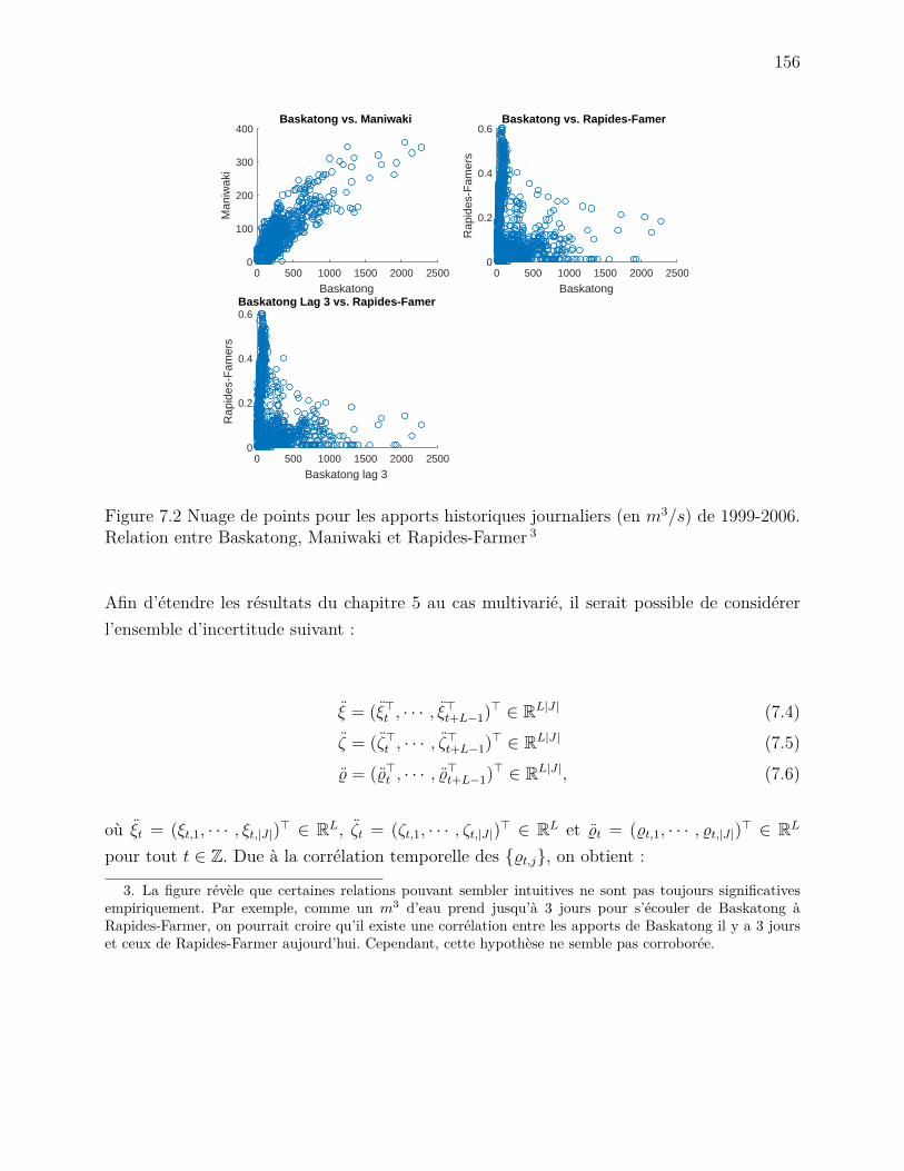
156

0 500 1000 1500 2000 25000

100

200

300

400

Man

iwak

i

Baskatong vs. Maniwaki

0 500 1000 1500 2000 2500

Baskatong

0

0.2

0.4

0.6

Rap

ides

-Fam

ers

Baskatong vs. Rapides-Famer

0 500 1000 1500 2000 2500

Baskatong lag 3

0

Rap

ides

-Fam

ers

BaskatongBaskatong Lag 3 vs. Rapides-Famer 0.6

0.4

0.2

Figure 7.2 Nuage de points pour les apports historiques journaliers (en m3/s) de 1999-2006.Relation entre Baskatong, Maniwaki et Rapides-Farmer 3

Afin d’étendre les résultats du chapitre 5 au cas multivarié, il serait possible de considérerl’ensemble d’incertitude suivant :

ξ = (ξ>t , · · · , ξ>t+L−1)> ∈ RL|J | (7.4)ζ = (ζ>t , · · · , ζ>t+L−1)> ∈ RL|J | (7.5)% = (%>t , · · · , %>t+L−1)> ∈ RL|J |, (7.6)

où ξt = (ξt,1, · · · , ξt,|J |)> ∈ RL, ζt = (ζt,1, · · · , ζt,|J |)> ∈ RL et %t = (%t,1, · · · , %t,|J |)> ∈ RL

pour tout t ∈ Z. Due à la corrélation temporelle des %t,j, on obtient :

3. La figure révèle que certaines relations pouvant sembler intuitives ne sont pas toujours significativesempiriquement. Par exemple, comme un m3 d’eau prend jusqu’à 3 jours pour s’écouler de Baskatong àRapides-Farmer, on pourrait croire qu’il existe une corrélation entre les apports de Baskatong il y a 3 jourset ceux de Rapides-Farmer aujourd’hui. Cependant, cette hypothèse ne semble pas corroborée.

157

E[%l%>k

]=

Σ ∈ R|J |×|J | if k = l

0 ∈ R|J |×|J | if k 6= l(7.7)

et donc :

E[%%>

]= Σ (7.8)

=

Σ · · · 0Σ ...

... . . .0 · · · Σ

∈ RL|J |×L|J |. (7.9)

Il devient ensuite possible de considérer l’ensemble d’incertitude suivant :

Ξt =

ξ ∈ RL|J |

∣∣∣∣∣∣∣∣∣∣∣∣∣

∃ζ , % ∈ RL|J |

ξ = Utζ + ut

ζ = Vt%+ vt

%>Σ−1% ≤ L|J |ε,

(7.10a)(7.10b)(7.10c)(7.10d)

où Ut, Vt ∈ RL|J |×L|J | sont des matrices creuses bloc angulaires ayant unestructure similaire à Σ et jouant un rôle semblable à celle dans la repré-sentation univariée du chapitre 5. On pourrait notamment considérer l’applica-tion Ut = diag(σt,1, · · · , σt,|J |, · · · , σt+L−1,1, · · · , σt+L−1,|J |) ∈ RL|J |×L|J | et ut =(µt,1, · · ·µt,|J |, · · · , µt+L−1,1, · · ·µt+L−1,|J |)> ∈ RL|J |, où σ2

t,j = E [(ξt,j − µt,j)2] et µt,j = E [ξt,j],qui est simplement la version multivariée de la transformation affine utilisée au chapitre 5.

Cependant, il n’est pas garanti que la matrice Σ−1 existe, car Σ et Σ ne sont pas nécessai-rement inversibles. il s’agit d’un exemple de difficulté additionnelle engendrée pas la naturemultidimensionnelle des séries chronologiques qui n’apparaissait pas dans le cas univarié.Dans le cas où Σ est de rang k < |J | ou presque singulière (ce qu’on peut notamment évaluerà l’aide d’une décomposition SVD et du nombre de conditionnement de la matrice), il estpossible de considérer k combinaisons linéaires indépendantes des ζt,∀t. On pourrait notam-ment utiliser l’analyse par composantes principales pour identifier les k combinaisons linéairesindépendants qui expliquent la plus grande variabilité des données. On peut ensuite effectuer

158

l’analyse par séries chronologiques sur les vecteurs aléatoires de dimension k appropriés.

On considère également la matrice suivante :

Vt =

I · · · 0Ψ1 I

...... . . .

ΨL−1 · · · Ψ1 I

∈ RL|J |×L|J |. (7.11)

Par exemple, dans le cas d’un modèle VAR(1)(vector autoregressive), on obtiendrait Ψi =Φi, i = 0, 1, · · · , L où Φ ∈ R|J |×|J | représente la matrice à calibrer en utilisant les données.

L’ellipse (7.10d) nous donne les mêmes garanties probabilistes qu’aux chapitres 5 et 6 :

P (%>Σ−1% > L|J |ε) ≤ tr(Σ−1E[%%>

])(L|J |ε)−1 (7.12)

=L∑l=1

tr(Σ−1E[%l%>l

])(L|J |ε)−1 (7.13)

= ε−1. (7.14)

Il serait possible d’obtenir une approximation polyhédrale conservatrice en utilisant les mêmetechniques que celles présentées aux chapitres 5 et 6. On pourrait plus spécifiquement utiliserl’inclusion :

y :∥∥∥Σ−1/2y

∥∥∥2≤√L|J |ε ⊂ y :

∥∥∥Σ−1/2y∥∥∥

1≤ L|J |

√ε ∩ y :

∥∥∥Σ−1/2y∥∥∥∞≤√L|J |ε (7.15)

présentée à l’annexe 5.8.1 en fixant y = Σ1/2% ⇔ Σ−1/2y = % 4 et en décomposant y en sapartie positive et négative : y = y+ − y− où y+, y− ∈ R|J |L+ . On obtient ensuite le polyhèdrelifté suivant, qui est une approximation conservatrice de l’ellipse (7.10d) :

4. En faisant l’hypothèse que Σ−1/2 existe.

159

Υ =

% ∈ RL|J |

+

∣∣∣∣∣∣∣∣∣∣∣∣∣∣∣∣

∃y+, y− ∈ R|J |L+

%i = Σ−1/2i (y+ − y−), ∀i = 1, · · · , L|J |

L|J |∑i=1

(y+i + y−i ) ≤ L|J |ε1/2

(y+i + y−i ) ≤ (L|J |ε)1/2, ∀i = 1, · · · , L|J |

.

(7.16a)(7.16b)

(7.16c)

(7.16d)

Bien qu’il existe peu de différences conceptuelles entre les ensembles d’incertitude pour lesséries chronologiques univariées et multivariées, on constate rapidement qu’il existe des dif-férences pratiques non-négligeables entre les deux approches. Outre le besoin d’éliminer lacolinéarité dans les ζt, il faut également considérer le fait que l’analyse multivariée est habi-tuellement beaucoup plus complexe que celle dans le cas univarié (Tsay, 2005). L’identificationd’un modèle adéquat, sa calibration ainsi que sa validation seront effectivement plus difficiles.

Par ailleurs, il faut prendre en compte les impacts de l’augmentation de la dimension del’incertitude. La sous-section suivante illustre que bien que l’augmentation de la taille del’équivalent déterministe soit polynomiale, car on passera de O(L) à O(L|J |) variables etcontraintes pour chaque contrainte dans le problème déterministe, il est fort probable quel’impact sur les temps de calcul sera assez important. Une seule résolution du modèle pourraitdemander quelques minutes, ce qui représente une augmentation significative par rapport auxquelques secondes nécessaires dans le cas univarié.

Il semble également possible d’utiliser un modèle multivarié semblable pour étendre les tra-vaux du chapitre 6 en considérant le logarithme des apports à chaque réservoir et chaquepériode. Toutefois, cette nouvelle représentation demanderait également un travail non né-gligeable.

7.3.3 Conséquence additionnelle d’une représentation plus fine des apports

Les représentations désagrégées proposées à la section 7.3 auront une conséquence majeuresur la tractabilité et les temps de calcul des problèmes. Par exemple, si on fait l’hypothèseque les règles de décision prennent la forme :

Xkt(ζ) = X 0kt +

J∑j′=1

T∑t′=1X j′t′

kt ζt′ , k ∈ Kt, (7.17)

il faut résoudre le problème suivant pour s’assurer que R(ζ) ≤ r, ∀ζt ∈ Zt,ν ,∀t, où Zt,ν est

160

décrit par l’équation (7.3) :

maxζ

R0 +T∑t′=1

|J |∑j′=1Rj′,t′ζj′,t′ ≤ q

s. t. (π+t′ ) ζj′,t′ ≤ νσj′,t′ , ∀j′ ∈ J, t′ = 1, · · · , T

(π−t′ ) − ζj′,t′ ≤ −minµj′,t′ , νσj′,t′, ∀j′ ∈ J, t′ = 1, · · · , T.

En prenant le dual on constate qu’on multiplie le nombre de variables et de contraintes par|J | par rapport au problème formulé à la section 4.9.1.

Or, il est essentiel de passer à la représentation (7.17) si on considère un ensemble de dimen-sion |J | comme Zt,ν . En effet, les contraintes de conservation de masse ne peuvent tenir si lagranularité des règles de décision est trop faible par rapport à celle de la représentation desapports.

Supposons que l’incertitude prenne la forme ξjt = µjt + ζjt et qu’elle soit donc représentéepar un vecteur de dimension |J | à chaque t. C’est notamment le cas si on considère Zt,ν ,∀tdécrit par (7.3). Supposons également pour les besoins de la contradiction qu’on conserve lareprésentation agrégée originale pour les règles de décision :

Xkt(ζ) = X 0kt +

T∑t′=1X t′

kt(∑j′∈J

ζj′t′), k ∈ Kt. (7.18)

Pour que les contraintes de conservation de masse (4.2) soient respectées pour tout ζt ∈ Zt,ν ,on doit s’assurer que la somme des coefficients des ζj′,t′ soit nulle et donc pour chaque j et t :

St′jt = t∑τ=1

[minδmax,τ−1∑

l=δminλlF t

′

i+τ−l −F t′

i+τ−l] β + β It′≤tIj′=j. (7.19)

On a donc un système linéaire à |J ||T | contraintes et seulement 3|T | variables qui n’a pas desolutions si |J | > 3. On conclut que si l’incertitude a la dimension |J | à chaque t, alors on nepeut conserver de règles de décision qui dépendent seulement de la variable aléatoire agrégée∑j ζjt à chaque t.

161

7.3.4 Utilisation d’un modèle hydrologique

Le domaine de la gestion hydrique bénéficie du fait que l’incertitude associée aux apportsest extrinsèque aux décisions prises. La fonte de neige et les précipitations sont effectivementindépendantes de la production hydroélectrique et des débits soutirés. Il existe par ailleurs uncouplage généralement assez faible entre les modèles d’optimisation et les représentations del’incertitude. Il est donc possible d’exploiter les nombreuses années de travail des hydrologuesen modélisation hydrologique. Il est notamment possible d’incorporer des modèles hydrolo-giques comme CEQUEAU ou HYDROTEL (Morin and Paquet, 2007; Fortin et al., 1995)développés par l’INRS-ETE au processus de prévision et d’optimisation d’un bassin versant.

Contrairement aux processus ARIMA, ces modèles permettent d’expliquer la relation entreles précipitations et les débits selon des équations physiques en s’appuyant sur le topologie duterrain, la composition du sol, certains facteurs comme l’humidité ainsi que divers indicateursmétéorologiques. Ils offrent donc une capacité prévisionnelle supérieure aux processus ARIMApour prévoir les débits lorsque les conditions hydrologiques sont différentes du passé (Turcotteet al., 2004). De tels modèles sont notamment utilisés de façon opérationnelle chez Rio Tintopour l’optimisation stochastique des centrales hydroélectriques (Côté and Leconte, 2015).

De tels modèles n’ont pas été utilisés dans cette thèse par souci de simplicité, par manquede connaissance de ces ressources et par manque de données. Il est fort à parier que cesmodèles permettraient d’améliorer la qualité prévisionnelles des apports de manière appré-ciable. Comme la prévision des apports représente un aspect central de la gestion des rivières,notamment pour le contrôle des inondations, ceci semble être un domaine de recherche pro-metteur.

Il serait peut-être possible de coupler les travaux effectués sur les processus ARIMA dans cettethèse aux modèles hydrologiques. En effet, il est possible que les erreur de prévision associéesau modèle hydrologique démontrent une certaine corrélation temporelle. Par exemple, il estpossible que le modèle prévoit systématiquement plus d’eau en été ou qu’ils ait tendance àen prévoir plus à un temps donné s’il en a déjà prévu durant la semaine passée.

7.3.5 Modélisation des courbes d’évacuation

Dans les trois chapitres 4 5 et 6, on utilise la représentation suivante pour les contraintesreliées aux courbes d’évacuation :

Lit(ζ) ≤ C 0i + C ∆

i Sj−(i)t(ζ), ∀i ∈ Ievac, t. (7.20)

162

Utiliser une telle représentation affine des volumes pour représenter les courbes d’évacuationest une approche assez naïve. Afin d’avoir une représentation plus réaliste, on pourrait mo-déliser le problème en utilisant des variables binaires. Pour chaque centrale i ∈ Ievac et tempst, on peut considérer Kit fonctions affines (hyperplans) et utiliser :

Lit(ζ) ≤ C 0i + C ∆

i,kSj−(i)t,k(ζ) +M(1− bit,k), ∀k ∈ 1, · · · , Kit (7.21a)Kit∑k=1

bit,k = 1 (7.21b)

bit,k ∈ 0, 1, ∀k ∈ 1, · · · , Kit (7.21c)

oùM est une grande constante, par exemple le déversé maximal associé au plus grand volumehistorique. Avec les courbes présentées à la section 4.6, il semble suffisant de considérerKit = 2,∀i ∈ Ievac, t ∈ T et on obtient ainsi un problème avec |Ievac|T variables entières.Dans notre étude de cas, |Ievac| = 4 et il est envisageable d’utiliser cette modélisation.

Des résultats numériques préliminaires on montré que les temps de calcul augmentaient defaçon modérée, mais notable, en considérant uniquement 2 segments à la centrale de Rapides-Farmer. Néanmoins, les temps de calcul demeurent raisonnables si on ne procède pas à lasimulation de la politique avec cette nouvelle modélisation.

7.3.6 Résolution en horizon roulant sur un plus long horizon et réplication dela politique de gestion

Tel que suggéré par Grégory Émiel et Pierre-Marc Rondeau d’Hydro-Québec Production, ilest intéressant d’évaluer le résultat de l’application de l’algorithme 6.1 sur un horizon longterme. En effet, notre modèle court terme dispose uniquement d’une vision assez myope dufutur à travers la fonction de valeur de l’eau. Il est donc possible que la politique de gestionsuggérée par notre modèle produisent des effets indésirables à long terme, par exemple levidage complet du réservoir pour éviter une inondation durant la période considérée parl’algorithme.

Des simulations ont été effectuées sur un horizon d’un an avec des apports historiques dansle but d’évaluer s’il était possible d’obtenir une évolution périodique des volumes similairesà celle engendrée historiquement et illustrée par la figure 1.5. En fixant ϕ dans l’équation∑t+L−1τ=t

((1− ϕ)Ofloodsτ + ϕOprodτ

)pour un certain ϕ ∈ [0, 1], on observe que les réservoirs

se vident ou se remplissent très rapidement, ce qui mène à plusieurs violations des bornes

163

supérieures ou inférieures sur les volumes sur un horizon annuel. Ces résultats semblaientindépendants des stocks d’eau initiaux.

Des modifications heuristiques de ϕt ∈ [0, 1] à chaque t selon la saison ou selon un processusde moyenne mobile (moving average) combinés à des variations des fonctions de valeur d’eaun’ont pas permis d’observer les comportements escomptés. Il semble donc qu’il faille passerplus de temps afin de créer un algorithme totalement automatique ne nécessitant aucuneintervention humaine. L’interaction entre les modèles court et moyen termes demeure unequestion ouverte d’une grande pertinence.

164

CHAPITRE 8 CONCLUSION

Cette thèse considère la gestion mensuelle de la rivière Gatineau en présence d’incertitude surles apports. Elle démontre que les règles de décision linéaires possèdent plusieurs avantagesimportants comme la facilité d’implémentation numérique, la rapidité de calcul et l’obten-tion directe d’une règle de gestion. Par ailleurs, cette technique permet de mieux modélisercertains phénomènes comme les longs délais d’écoulement et la persistance des apports qued’autres techniques alternatives populaires comme la programmation dynamique stochastiqueclassique.

Les résultats des chapitres 4, 5 et 6 indiquent que les règles de décision linéaires peuvent êtreutilisées avec succès pour faciliter la gestion de la rivière Gatineau lorsque combinées avecun modèle de l’incertitude ayant une bonne capacité prédictive.

La section 7 illustre plusieurs pistes de solutions permettant de raffiner l’approche et decorriger certaines de ses limitations. Cependant, ces extensions auront probablement desconséquences assez importantes sur la clarté et la formulation du modèle, en plus d’entraînerdes augmentations de temps de calcul conséquentes.

165

RÉFÉRENCES

Aasgård, E., Andersen, G., Fleten, S.-F., and Haugstvedt, D. (2014). Evaluating astochastic-programming-based bidding model for a multireservoir system. IEEE Transac-tions on Power Systems, 29(4) :1748–1757.

Acciacio, B. and Penner, I. (2011). Advanced mathematical methods for finance, chapterDynamic Risk Measures, pages 1–34. Springer.

Acerbi, C. and Tasche, D. (2002). On the coherence of expected shortfall. Journal of Bankingand Finance, 26 :1487–1503.

Akaike, H. (1973). Information theory and an extension of the maximum likelihood principle.In Petrov, B. N. and Csaki, F., editors, Second International Symposium on InformationTheory, pages 267–281, Budapest. Akadémiai Kiado.

Apparigliato, R. (2008). Règles de décision pour la gestion du risque : Application à lagestion hebdomadaire de la production électrique. PhD thesis, École Polytechnique.

Ardestani-Jaafari, A. and Delage, E. (2014). The value of flexibility in robust locationtransportation problem. Technical Report G201483, Les cahiers du GERAD.

Armbruster, B. and Delage, E. (2015). Decision making under uncertainty when preferenceinformation is incomplete. Management Science, 61(1) :111–128.

Artus, V., . Durlofsky, L., & Onwunalu, J., and Aziz, K. (2006). Optimization of non-conventional wells under uncertainty using statistical proxies. Computational Geosciences,10(4) :389–404.

Artzner, P., Delbaen, F., Eber, J.-M., and Heath, D. (1999). Coherent measures of risk.Mathematical Finance, 9(3) :203–228.

Babaei, M., Pan, I., and Alkhatib, A. (2015). Robust optimization of well location toenhance hysteretical trapping of co2 : Assessment of various uncertainty quantification me-thods and utilization of mixed response surface surrogates. Water Resources Research,51(2015WR017418) :9402–9424.

Bana e Costa, C. A. and Vansnick, J.-C. (1997). A Theoretical Framework for MeasuringAttractiveness by a Categorical Based Evaluation Technique (MACBETH), pages 15–24.Springer Berlin Heidelberg, Berlin, Heidelberg.

Ben-Tal, A., El Ghaoui, L., and Nemirovski, A. (2009). Robust Optimization. PrincetonUniversity Press.

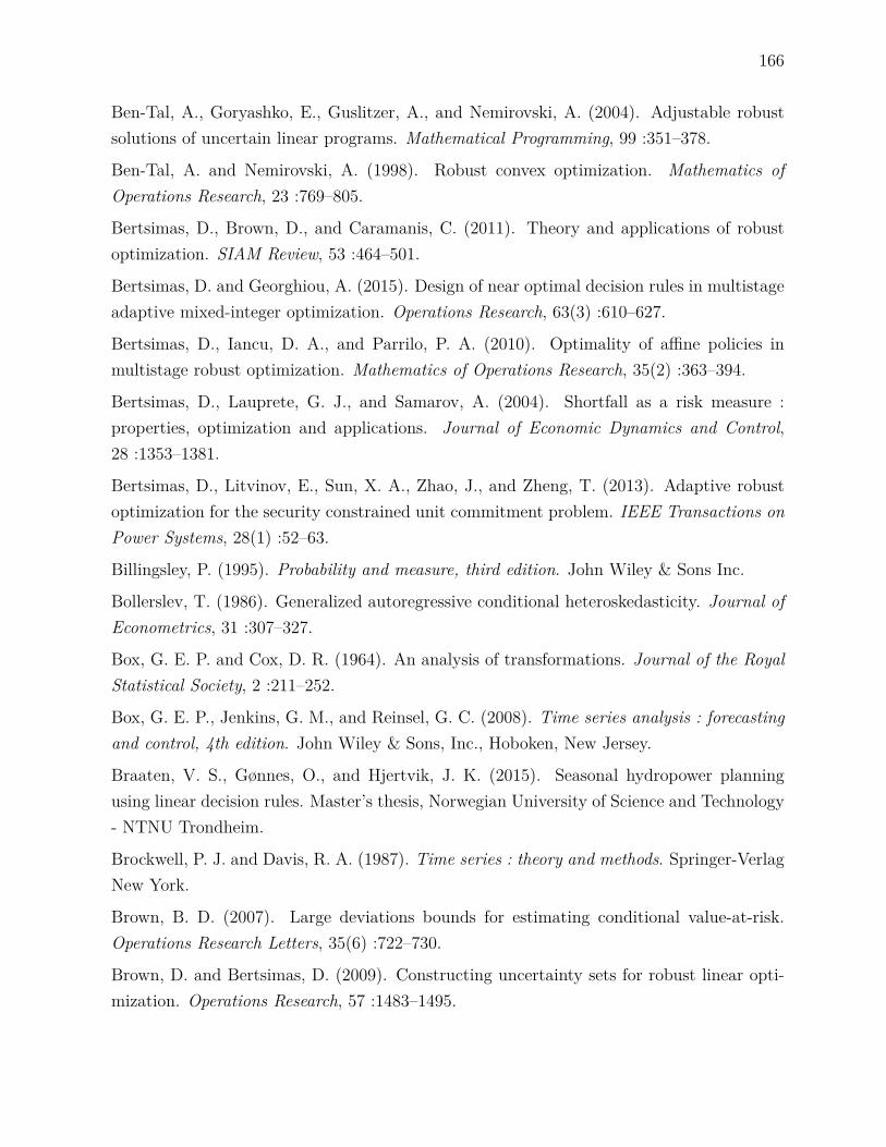
166

Ben-Tal, A., Goryashko, E., Guslitzer, A., and Nemirovski, A. (2004). Adjustable robustsolutions of uncertain linear programs. Mathematical Programming, 99 :351–378.

Ben-Tal, A. and Nemirovski, A. (1998). Robust convex optimization. Mathematics ofOperations Research, 23 :769–805.

Bertsimas, D., Brown, D., and Caramanis, C. (2011). Theory and applications of robustoptimization. SIAM Review, 53 :464–501.

Bertsimas, D. and Georghiou, A. (2015). Design of near optimal decision rules in multistageadaptive mixed-integer optimization. Operations Research, 63(3) :610–627.

Bertsimas, D., Iancu, D. A., and Parrilo, P. A. (2010). Optimality of affine policies inmultistage robust optimization. Mathematics of Operations Research, 35(2) :363–394.

Bertsimas, D., Lauprete, G. J., and Samarov, A. (2004). Shortfall as a risk measure :properties, optimization and applications. Journal of Economic Dynamics and Control,28 :1353–1381.

Bertsimas, D., Litvinov, E., Sun, X. A., Zhao, J., and Zheng, T. (2013). Adaptive robustoptimization for the security constrained unit commitment problem. IEEE Transactions onPower Systems, 28(1) :52–63.

Billingsley, P. (1995). Probability and measure, third edition. John Wiley & Sons Inc.

Bollerslev, T. (1986). Generalized autoregressive conditional heteroskedasticity. Journal ofEconometrics, 31 :307–327.

Box, G. E. P. and Cox, D. R. (1964). An analysis of transformations. Journal of the RoyalStatistical Society, 2 :211–252.

Box, G. E. P., Jenkins, G. M., and Reinsel, G. C. (2008). Time series analysis : forecastingand control, 4th edition. John Wiley & Sons, Inc., Hoboken, New Jersey.

Braaten, V. S., Gønnes, O., and Hjertvik, J. K. (2015). Seasonal hydropower planningusing linear decision rules. Master’s thesis, Norwegian University of Science and Technology- NTNU Trondheim.

Brockwell, P. J. and Davis, R. A. (1987). Time series : theory and methods. Springer-VerlagNew York.

Brown, B. D. (2007). Large deviations bounds for estimating conditional value-at-risk.Operations Research Letters, 35(6) :722–730.

Brown, D. and Bertsimas, D. (2009). Constructing uncertainty sets for robust linear opti-mization. Operations Research, 57 :1483–1495.

167

Carpentier, P.-L., Gendreau, M., and Bastin, F. (2013a). Long-term management of a hy-droelectric multireservoir system under uncertainty using the progressive hedging algorithm.Water Resources Research, 49 :2812–2827.

Carpentier, P.-L., Gendreau, M., and Bastin, F. (2013b). Optimal scenario set partitioningfor multistage stochastic programming with the progressive hedging algorithm. TechnicalReport CIRRELT-2013-55, CIRRELT.

Carpentier, P.-L., Gendreau, M., and Bastin, F. (2015). Managing hydroelectric reservoirsover an extended horizon using benders decomposition with a memory loss assumption.IEEE Transactions on Power Systems, 30(2) :563–572.

Castelletti, A., Galelli, S., Restelli, M., and Soncini-Sessa, R. (2012). Data-driven dynamicemulation modelling for the optimal management of environmental systems. EnvironmentalModelling & Software, 34 :30 – 43. Emulation techniques for the reduction and sensitivityanalysis of complex environmental models.

Castelletti, A., Galetti, S., Restelli, M., and Soncini-Sessa, R. (2010). Tree-based reinforce-ment learning for optimal water reservoir operation. Water Resources Research, 46 :W09507.

Castelletti, A., Pianosi, F., and Soncini-Sessa, R. (2008). Water reservoir control undereconomic, social and environmental constraints. Automatica, 44(6) :1595–1607.

Castillo, A., Lipka, P., Watson, J. P., Oren, S. S., and O’Neill, R. P. (2016). A successivelinear programming approach to solving the iv-acopf. IEEE Transactions on Power Systems,31(4) :2752–2763.

Cervellera, C., Chen, V., and Wen, A. (2006). Optimization of a large-scale water reser-voir network by stochastic dynamic programming with efficient state space discretization.European Journal of Operational Research, 171 :1139–1151.

Chen, W., Sim, M., Sun, J., and Teo, C.-P. (2010). From cvar to uncertainty set : implicationsin joint chance-constrained optimization. Operations Research, 58 :470–485.

Chen, X., Sim, M., Sun, P., and Zhang, J. (2008). A linear decision-based approximationapproach to stochastic programming. Operations Research, 56 :344–357.

Commission de toponymie : Gouvernement du Québec (2017). Rivière gatineau.

Côté, P. (2010). Gestion d’un ensemble d’installations hydroélèctriques soumis á unecontrainte de demande. PhD thesis, École Polytechnique de Montréal.

Côté, P., Haguma, D., Leconte, R., and Krau, S. (2011). Stochastic optimisation of hydro-quebec hydropower installations : a statistical comparison between sdp and ssdp methods.Revue canadienne de génie civil, 38(12) :1427–1434.

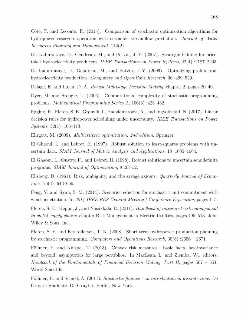
168

Côté, P. and Leconte, R. (2015). Comparison of stochastic optimization algorithms forhydropower reservoir operation with ensemble streamflow prediction. Journal of WaterResources Planning and Management, 142(2).

De Ladurantaye, D., Gendreau, M., and Potvin, J.-Y. (2007). Strategic bidding for price-taker hydroelectricity producers. IEEE Transactions on Power Systems, 22(4) :2187–2203.

De Ladurantaye, D., Gendreau, M., and Potvin, J.-Y. (2009). Optimizing profits fromhydroelectricity production. Computers and Operations Research, 36 :499–529.

Delage, E. and Iancu, D. A. Robust Multistage Decision Making, chapter 2, pages 20–46.

Dyer, M. and Stougie, L. (2006). Computational complexity of stochastic programmingproblems. Mathematical Programming Series A, 106(3) :423–432.

Egging, R., Fleten, S. E., Grønvik, I., Hadziomerovic, A., and Ingvoldstad, N. (2017). Lineardecision rules for hydropower scheduling under uncertainty. IEEE Transactions on PowerSystems, 32(1) :103–113.

Ehrgott, M. (2005). Multicriteria optimization, 2nd edition. Springer.

El Ghaoui, L. and Lebret, H. (1997). Robust solution to least-squares problems with un-certain data. SIAM Journal of Matrix Analysis and Applications, 18 :1035–1064.

El Ghaoui, L., Oustry, F., and Lebret, H. (1998). Robust solutions to uncertain semidefiniteprograms. SIAM Journal of Optimization, 9 :33–52.

Ellsberg, D. (1961). Risk, ambiguity, and the savage axioms. Quarterly Journal of Econo-mics, 75(4) :643–669.

Feng, Y. and Ryan, S. M. (2014). Scenario reduction for stochastic unit commitment withwind penetration. In 2014 IEEE PES General Meeting | Conference Exposition, pages 1–5.

Fleten, S.-E., Keppo, J., and Näsäkkälä, E. (2011). Handbook of integrated risk managementin global supply chains, chapter Risk Management in Electric Utilities, pages 495–513. JohnWiley & Sons, Inc.

Fleten, S.-E. and Kristoffersen, T. K. (2008). Short-term hydropower production planningby stochastic programming. Computers and Operations Research, 35(8) :2656 – 2671.

Föllmer, H. and Knispel, T. (2013). Convex risk measures : basic facts, law-invarianceand beyond, asymptotics for large portfolios. In MacLean, L. and Ziemba, W., editors,Handbook of the Fundamentals of Financial Decision Making, Part II, pages 507 – 554.World Scientific.

Föllmer, H. and Schied, A. (2011). Stochastic finance : an introduction in discrete time. DeGruyter graduate. De Gruyter, Berlin, New York.

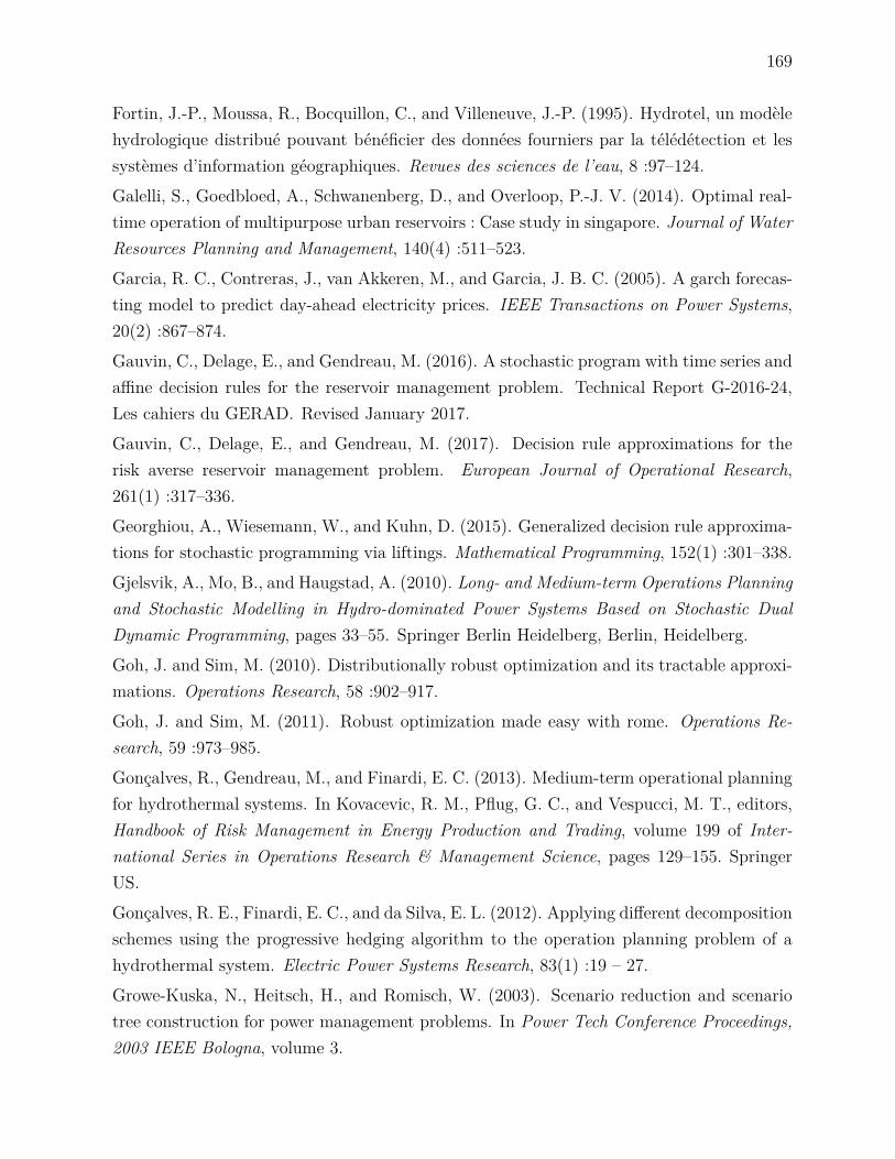
169

Fortin, J.-P., Moussa, R., Bocquillon, C., and Villeneuve, J.-P. (1995). Hydrotel, un modèlehydrologique distribué pouvant bénéficier des données fourniers par la télédétection et lessystèmes d’information géographiques. Revues des sciences de l’eau, 8 :97–124.Galelli, S., Goedbloed, A., Schwanenberg, D., and Overloop, P.-J. V. (2014). Optimal real-time operation of multipurpose urban reservoirs : Case study in singapore. Journal of WaterResources Planning and Management, 140(4) :511–523.Garcia, R. C., Contreras, J., van Akkeren, M., and Garcia, J. B. C. (2005). A garch forecas-ting model to predict day-ahead electricity prices. IEEE Transactions on Power Systems,20(2) :867–874.Gauvin, C., Delage, E., and Gendreau, M. (2016). A stochastic program with time series andaffine decision rules for the reservoir management problem. Technical Report G-2016-24,Les cahiers du GERAD. Revised January 2017.Gauvin, C., Delage, E., and Gendreau, M. (2017). Decision rule approximations for therisk averse reservoir management problem. European Journal of Operational Research,261(1) :317–336.Georghiou, A., Wiesemann, W., and Kuhn, D. (2015). Generalized decision rule approxima-tions for stochastic programming via liftings. Mathematical Programming, 152(1) :301–338.Gjelsvik, A., Mo, B., and Haugstad, A. (2010). Long- and Medium-term Operations Planningand Stochastic Modelling in Hydro-dominated Power Systems Based on Stochastic DualDynamic Programming, pages 33–55. Springer Berlin Heidelberg, Berlin, Heidelberg.Goh, J. and Sim, M. (2010). Distributionally robust optimization and its tractable approxi-mations. Operations Research, 58 :902–917.Goh, J. and Sim, M. (2011). Robust optimization made easy with rome. Operations Re-search, 59 :973–985.Gonçalves, R., Gendreau, M., and Finardi, E. C. (2013). Medium-term operational planningfor hydrothermal systems. In Kovacevic, R. M., Pflug, G. C., and Vespucci, M. T., editors,Handbook of Risk Management in Energy Production and Trading, volume 199 of Inter-national Series in Operations Research & Management Science, pages 129–155. SpringerUS.Gonçalves, R. E., Finardi, E. C., and da Silva, E. L. (2012). Applying different decompositionschemes using the progressive hedging algorithm to the operation planning problem of ahydrothermal system. Electric Power Systems Research, 83(1) :19 – 27.Growe-Kuska, N., Heitsch, H., and Romisch, W. (2003). Scenario reduction and scenariotree construction for power management problems. In Power Tech Conference Proceedings,2003 IEEE Bologna, volume 3.

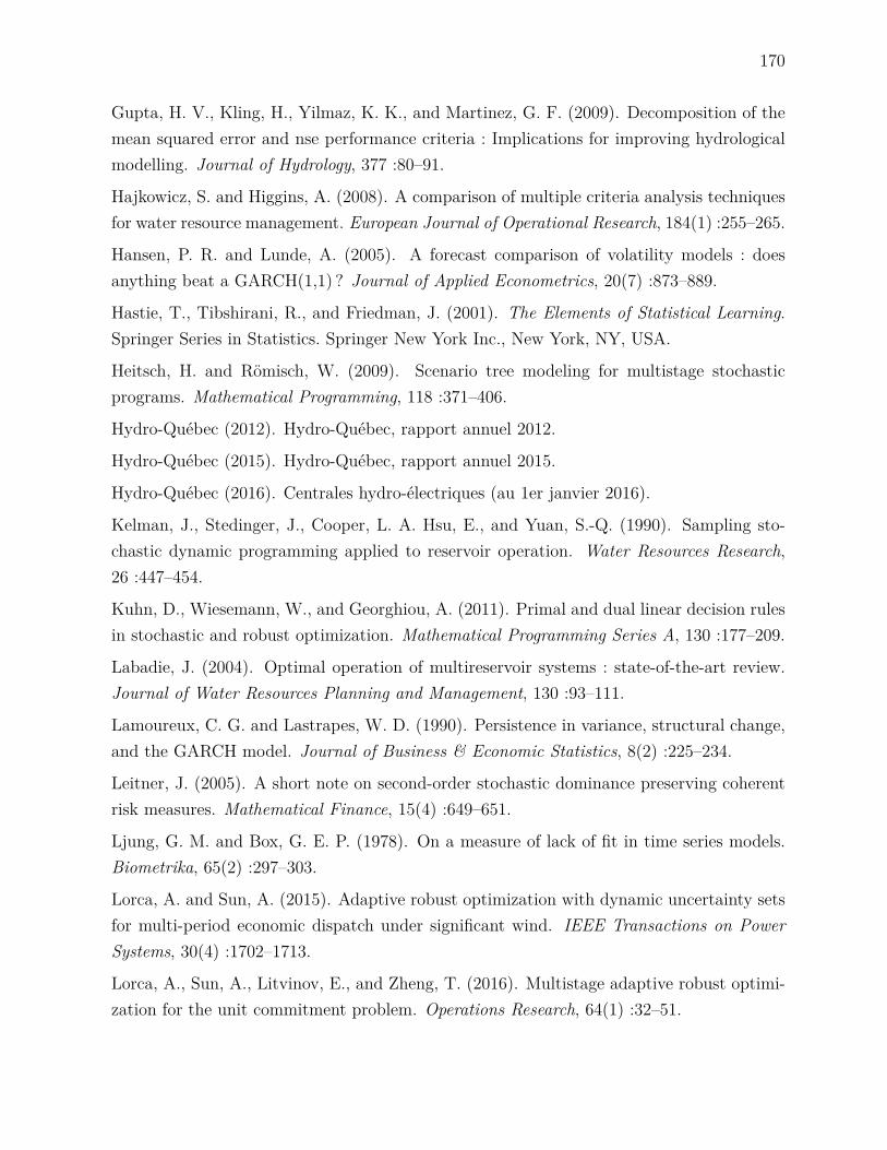
170

Gupta, H. V., Kling, H., Yilmaz, K. K., and Martinez, G. F. (2009). Decomposition of themean squared error and nse performance criteria : Implications for improving hydrologicalmodelling. Journal of Hydrology, 377 :80–91.

Hajkowicz, S. and Higgins, A. (2008). A comparison of multiple criteria analysis techniquesfor water resource management. European Journal of Operational Research, 184(1) :255–265.

Hansen, P. R. and Lunde, A. (2005). A forecast comparison of volatility models : doesanything beat a GARCH(1,1) ? Journal of Applied Econometrics, 20(7) :873–889.

Hastie, T., Tibshirani, R., and Friedman, J. (2001). The Elements of Statistical Learning.Springer Series in Statistics. Springer New York Inc., New York, NY, USA.

Heitsch, H. and Römisch, W. (2009). Scenario tree modeling for multistage stochasticprograms. Mathematical Programming, 118 :371–406.

Hydro-Québec (2012). Hydro-Québec, rapport annuel 2012.

Hydro-Québec (2015). Hydro-Québec, rapport annuel 2015.

Hydro-Québec (2016). Centrales hydro-électriques (au 1er janvier 2016).

Kelman, J., Stedinger, J., Cooper, L. A. Hsu, E., and Yuan, S.-Q. (1990). Sampling sto-chastic dynamic programming applied to reservoir operation. Water Resources Research,26 :447–454.

Kuhn, D., Wiesemann, W., and Georghiou, A. (2011). Primal and dual linear decision rulesin stochastic and robust optimization. Mathematical Programming Series A, 130 :177–209.

Labadie, J. (2004). Optimal operation of multireservoir systems : state-of-the-art review.Journal of Water Resources Planning and Management, 130 :93–111.

Lamoureux, C. G. and Lastrapes, W. D. (1990). Persistence in variance, structural change,and the GARCH model. Journal of Business & Economic Statistics, 8(2) :225–234.

Leitner, J. (2005). A short note on second-order stochastic dominance preserving coherentrisk measures. Mathematical Finance, 15(4) :649–651.

Ljung, G. M. and Box, G. E. P. (1978). On a measure of lack of fit in time series models.Biometrika, 65(2) :297–303.

Lorca, A. and Sun, A. (2015). Adaptive robust optimization with dynamic uncertainty setsfor multi-period economic dispatch under significant wind. IEEE Transactions on PowerSystems, 30(4) :1702–1713.

Lorca, A., Sun, A., Litvinov, E., and Zheng, T. (2016). Multistage adaptive robust optimi-zation for the unit commitment problem. Operations Research, 64(1) :32–51.

171

Loucks, D. P. and Dorfman, P. J. (1975). An evaluation of some linear decision rules inchance-constrained models for reservoir planning and operation. Water Resources Research,11 :777–785.

Maceira, M. and Damázio, J. (2004). The use of par(p) model in the stochastic dualdynamic programming optimization scheme used in the operation planning of the brazilianhydropower system. 8th International Conference on Probabilistic Methods Applied toPower Systems, pages 397–402. Iowa State University.

Morin, G. and Paquet, P. (2007). Modèle hydrologique cequeau. Technical report, INRS-ETE.

Nash, J. and Sutcliffe, J. (1970). River flow forecasting through conceptual models. part i.- a discussion of principles. Journal of Hydrology, 10 :282–290.

Natarajan, N., Pachamanova, D., and Sim, M. (2009). Constructing risk measures fromuncertainty sets. Operations Research, 57 :1129–1141.

Neumann, J. v. and Morgenstern, O. (1953). Theory of Games and Economic Behavior(Third ed.). Princeton, NJ : Princeton University Press.

Nocedal, J. and Wright, S. J. (2006). Numerical Optimization, 2nd Edition. Springer Seriesin Operations Research. Springer.

Palacios-Gomez, F., Lasdon, L., and Engquist, M. (1982). Nonlinear optimization by suc-cessive linear programming. Management Science, 28(10) :1106–1120.

Pan, L., Housh, M., Liu, P., Cai, X., and Chen, X. (2015). Robust stochastic optimizationfor reservoir operation. Water Resources Research, 51(1) :409–429.

Pereira, M. and Pinto, L. (1991). Multi-stage stochastic optimization applied to energyplanning. Mathematical Programming, 52 :359–375.

Pflug, G. (2000). Some remarks on the value-at-risk and the conditional value-at-risk.In Uryasev, S., editor, Probabilistic Constrained Optimization, volume 49 of NonconvexOptimization and Its Applications, pages 272–281. Springer US.

Pflug, G. and Pichler, A. (2016). From empirical observations to tree models for stochasticoptimization : Convergence properties. SIAM Journal on Optimization, 26(3) :1715–1740.

Phillpot, A. and Guan, Z. (2008). On the convergence of stochastic dual dynamic program-ming and related methods. Operations Research Letters, 36.

Pianosi, F. and Soncini-Sessa, R. (2009). Real-time management of a multipurpose waterreservoir with a heteroscedastic inflow model. Water Resources Research, 45(10) :1–12.W10430.

172

Pina, J., Tilmant, A., and Anctil, F. (2016). Horizontal approach to assess the impactof climate change on water resources systems. Journal of Water Resources Planning andManagement.

Powell, W. B. (2007). Approximate dynamic programming : solving the curses of dimensio-nality. Wiley.

Quentin, D., Côté, P. P., and Robert, L. (2014). Role of hydrologic information in stochasticdynamic programming : a case study of the kemano hydropower system in british columbia.Canadian Journal of Civil Engineering/Revue canadienne de génie civil, 41(9) :839–844.

ReVelle, C. S. and Kirby, W. (1970). Linear decision rule in reservoir management anddesign, 2, performance optimization. Water Resources Research, 6 :1033–1044.

Riedel, F. (2004). Dynamic coherent risk measures. Stochastic Processes and their Applica-tions, 112 :185–200.

Rocha, P. and Kuhn, D. (2012). Multistage stochastic portfolio optimisation in deregulatedelectricity markets using linear decision rules. European Journal of Operational Research,216(2) :397–408.

Rockafellar, R. and Wets, R. (1991). Scenarios and policy aggregation in optimization underuncertainty. Mathematics of Operations Research, 16 :119–147.

Rockafellar, T. R. and Uryasev, S. (2002). Conditional value-at-risk for general loss distri-butions. Journal of Banking and Finance, 26 :1443–1471.

Romanowicz, R. J., Young, P. C., and Beven, K. J. (2006). Data assimilation and adaptiveforecasting of water levels in the river severn catchment, united kingdom. Water ResourcesResearch, 42(6). W06407.

Rönnqvist, M. (2003). Optimization in forestry. Mathematical Programming, 97(1) :267–284.

Rougé, C. and Tilmant, A. (2016). Using stochastic dual dynamic programming in problemswith multiple near-optimal solutions. Water Resources Research, 52(5) :4151–4163.

Rudin, W. (1987). Real and Complex Analysis, 3rd Ed. McGraw-Hill, Inc., New York, NY,USA.

Saad, M., Bigras, P., and Turgeon, A. (1996). Fuzzy learning decomposition for the sche-duling of hydroelectric power system. Water Resources Research, 32 :179–186.

Saad, M. and Turgeon, A. (1988). Application of principal component anbalysis to long-termreservoir management. Water Resources Research, 24 :907–912.

Saddoune, M. (2010). Optimisation simultanée des rotations et des blocs mensuels deséquipages aériens. PhD thesis, École Polytechnique de Montréal.

173

Salas, J. D., Delleur, J. W., Yevjevich, V., and Lane, W. L. (1980). Applied modeling ofhydrologic time series. Water Resources Publications, Littleton, Colorado.

Séguin, S. (2016). Optimisation stochastique de la répartition spatio-temporelle d’un volumed’eau aux groupes turbo-alternateurs d’un système de production hydroélectrique. PhD thesis,École Polytechnique de Montréal.

Séguin, S., Côté, P., and Audet, C. (2016a). Self-scheduling short-term unit commitmentand loading problem. IEEE Transactions on Power Systems, 31(1) :133–142.

Séguin, S., Fleten, S.-E., Côté, P., Pichler, A., and Audet, C. (2016b). Stochastic short-termhydropower planning with inflow scenario trees. European Journal of Operational Research,259(3) :156–1168.

Shapiro, A. (2009). On a time consistency concept in risk averse multistage stochasticprogramming. Operations Research Letters, 37(3) :143 – 147.

Shapiro, A. (2011). Analysis of stochastic dual dynamic programming method. EuropeanJournal of Operational Research, 209 :63–72.

Shapiro, A., Dentcheva, D., and Ruszcyński, A. (2009). Lectures on stochastic programming :modeling and theory. MOS-SIAM Series on Optimization.

Shapiro, A., Tekaya, W., da Costa, J. P., and Soares, M. P. (2013). Risk neutral and riskaverse stochastic dual dynamic programming method. European Journal of OperationalResearch, 224(2) :375 – 391.

Sim, M. and Bertsimas, D. (2004). The price of robustness. Operations Research, 52(1) :35–53.

Soyster, A. (1973). Convex programming with set-inclusive constraints and applications toinexact linear programming. Operations Research, 21(5) :1154–1157.

Stedinger, J. (1984). The performance of ldr models for preliminary design and reservoiroperation. Water Resources Research, 20 :215–224.

Stedinger, J. R. and Faber, B. A. (2001). Reservoir optimization using sampling sdp withensemble streamflow prediction (esp) forecast. Journal of Hydrology, 249 :113–133.

Tandberg, C. and Vefring, E. S. (2012). The linear decision rule approach applied to thehydrothermal generation planning problem. Master’s thesis, Norwegian University of Scienceand Technology - NTNU Trondheim.

Tejada-Guibert, J. A., Johnson, S. A., and Stedinger, J. R. (1995). The value of hydrologicinformation in stochastic dynamic programming models of a multireservoir system. WaterResources Research, 31(10) :2571–2579.

174

Tilmant, A. and Kelman, R. (2007). A stochastic approach to analyze trade-offs and riskassociated with large-scale water resources systems. Water Resources Research, 43 :W06425.

Tsay, R. S. (2005). Analysis of Financial Time Series, Second Edition. John Wiley & Sons,Inc., Hoboken, New Jersey.

Turcotte, R., Lacombe, P., Dimnik, C., and Villeneuve, J.-P. (2004). Prévision hydrolo-gique distribuée pour la gestion des barrages publics du québec. Canadian Journal of CivilEngineering/Revue canadienne de génie civil, 31(2) :308–320.

Turgeon, A. (2005). Solving a stochastic reservoir management problem with multilagautocorrelated inflows. Water Resources Research, 41 :W12414.

Turgeon, A. (2007). Stochastic optimization of multireservoir operation : The optimal re-servoir trajectory approach. Water Resources Research, 43 :W05420.

Turgeon, A. and Charbonneau, R. (1998). An aggregation-disaggregation approach to long-term reservoir management. Water Resources Research, 34 :3585–3594.

Wood, A. W. and Schaake, J. C. (2008). Correcting errors in streamflow forecast ensemblemean and spread. Journal of hydrometeorology, 9 :132–174.

Yeh, W. W.-G. (1985). Reservoir management and operations models : A state-of-the-artreview. Water Resources Research, 21(12) :1797–1818.

Yuan, Y.-x. (2015). Recent advances in trust region algorithms. Mathematical ProgrammingSeries B, 151(1) :249–281.

Zéphyr, L., Lang, P., Lamond, B. F., and Côté, P. (2016). Controlled Approximation ofthe Stochastic Dynamic Programming Value Function for Multi-Reservoir Systems, pages31–37. Springer International Publishing, Cham.