model structures and structural identifiability: what? why? how?
TRANSCRIPT
Model structures and structural identifiability:What? Why? How?
Jason M. Whyte
Abstract We may attempt to encapsulate what we know about a physical systemby a model structure, S. This collection of related models is defined by parametricrelationships between system features; say observables (outputs), unobservable vari-ables (states), and applied inputs. Each parameter vector in some parameter spaceis associated with a completely specified model in S. Before choosing a model in Sto predict system behaviour, we must estimate its parameters from system observa-tions. Inconveniently, multiple models (associated with distinct parameter estimates)may approximate data equally well. Yet, if these equally valid alternatives producedissimilar predictions of unobserved quantities, then we cannot confidently makepredictions. Thus, our study may not yield any useful result.
We may anticipate the non-uniqueness of parameter estimates ahead of data col-lection by testing S for structural global identifiability (SGI). Here we will providean overview of the importance of SGI, some essential theory and distinctions, anddemonstrate these in testing some examples.
1 Introduction
A “model structure” (or simply “structure”) is essentially a collection of relatedmodels of some particular class (say the linear, first-order, homogeneous, constant-coefficient ODEs in n variables), as summarised by mathematical relationships be-tween system variables that depend on parameters. For example, in a “controlledstate-space structure” we may draw on our knowledge of the system to relate time-varying quantities such as “states” (x) that we may not be able to observe, and(typically known) controls or “inputs” (u) which act on some part of our system,to “outputs” (y) we can observe. A structure is a useful construct when seeking to
Jason M. WhyteACEMS, School of Mathematics and Statistics, and CEBRA, School of BioSciences, Universityof Melbourne, Parkville Victoria, Australia, 3010, e-mail: [email protected]
1
2 Jason M. Whyte
model some physical system for which our knowledge is incomplete. We choosesome suitable parameter space, and each parameter vector therein is associated witha model in our structure, where we use “model” to mean a completely specified setof mathematical relationships between system variables.
In order to illustrate the concept of a structure, we will consider S1, a controlledstate-space structure of “compartmental” models, meaning that these are subject toa “conservation of mass” condition—matter is neither created nor destroyed. Whenwe are interested in a system evolving in continuous time, a structure will employ or-dinary differential equations (ODEs) to describe the time course of the states. Com-partmental structures are often appropriate for the modelling of biological systems.To illustrate this, let us consider a simple biochemical system, where we considerthe interconversion and consumption of chemical species, as in a cellular process.Structure S1 has three states, x1, x2, and x3, representing concentrations of threedistinct chemical species, or “compartments”. Matter may be excreted from the sys-tem, delivered into the system, or converted between the forms. We assume that thesystem receives some infusion of x3 via input u.
Using standard notation for compartmental systems, a real parameter ki j (i, j =1,2,3, i 6= j) represents the rate constant for the conversion of x j into xi. A realparameter k0 j is the rate constant associated with the loss of material from x j tothe “environment” outside of the system. If reactions are governed by “first-ordermass-action kinetics”, the rate of conversion (or excretion) of some species at timet depends linearly on the amount of that species at time t.
Given our physical system and modelling paradigm, (and understanding that anexpression such as x represents dx/dt) we may write the “representative model” ofS1 as
x1(t) =−(k01 + k21)x1(t)− k12x2(t) ,
x2(t) = k21x1(t)− (k12 + k32)x2(t)+ k23x3(t) ,
x3(t) = k32x2(t)− k23x3(t)+u(t) ,(1)
where we set initial conditions for our states (where > denotes transpose)(x1(0) x2(0) x3(0)
)>=(0 x20 0
)>. (2)
Supposing that x1 is the only state we can observe over time, our output isy(t) = x1(t) . (3)
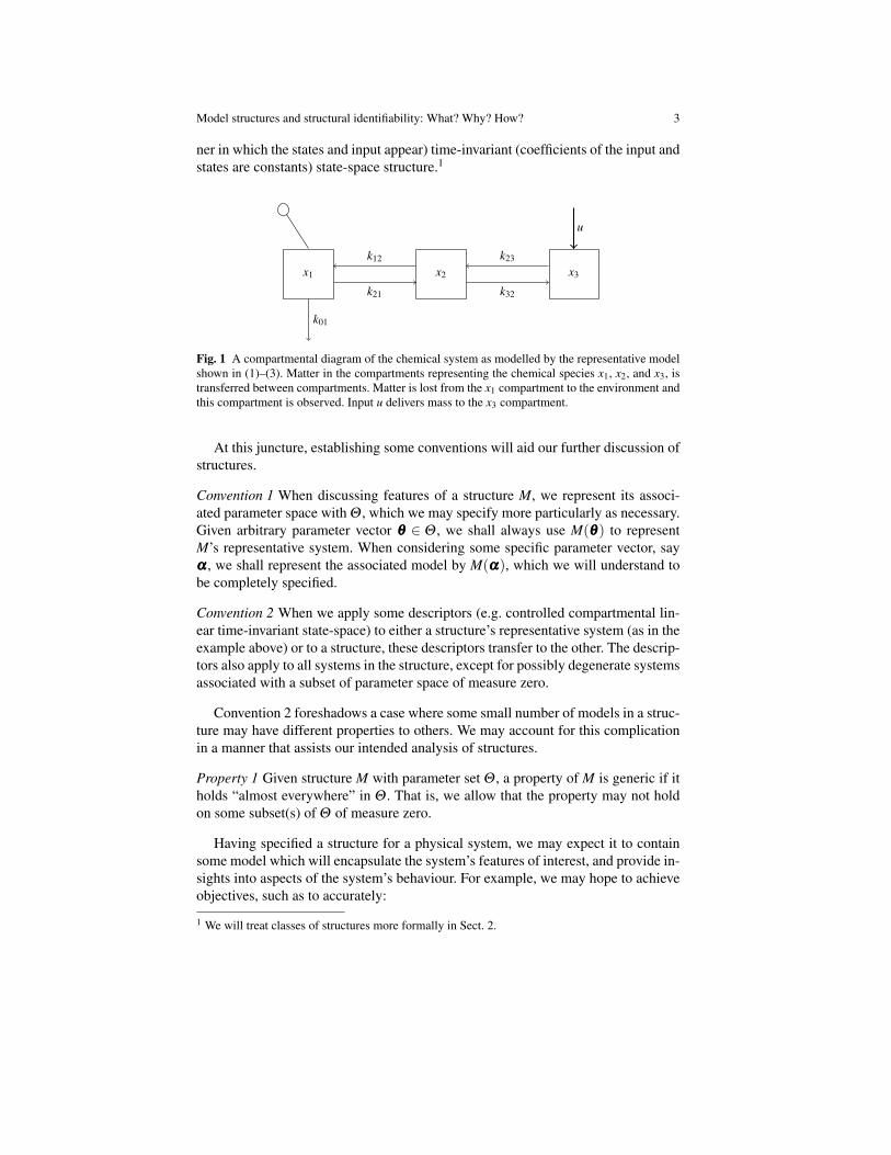
We may represent this “single-input single-output” (SISO) structure by a com-partmental diagram, as in Figure 1. Squares represent distinct chemical species, thinarrows show the conversion of mass to other forms, or excretion from the system.The rates of conversion or excretion are determined by the product of the associatedparameter and the state variable at the source of the arrow. The thick arrow shows aninput, and the circle linked to x1 indicates that this compartment is observed. Morespecifically, Figure 1, (1), and (3) illustrate the representative model of a controlled(due to the input u) compartmental (mass is conserved) linear (describing the man-
Model structures and structural identifiability: What? Why? How? 3
ner in which the states and input appear) time-invariant (coefficients of the input andstates are constants) state-space structure.1
x2x1 x3
k21
k12
k32
k23
k01
u
Fig. 1 A compartmental diagram of the chemical system as modelled by the representative modelshown in (1)–(3). Matter in the compartments representing the chemical species x1, x2, and x3, istransferred between compartments. Matter is lost from the x1 compartment to the environment andthis compartment is observed. Input u delivers mass to the x3 compartment.
At this juncture, establishing some conventions will aid our further discussion ofstructures.
Convention 1 When discussing features of a structure M, we represent its associ-ated parameter space with Θ , which we may specify more particularly as necessary.Given arbitrary parameter vector θθθ ∈ Θ , we shall always use M(θθθ) to representM’s representative system. When considering some specific parameter vector, sayααα , we shall represent the associated model by M(ααα), which we will understand tobe completely specified.
Convention 2 When we apply some descriptors (e.g. controlled compartmental lin-ear time-invariant state-space) to either a structure’s representative system (as in theexample above) or to a structure, these descriptors transfer to the other. The descrip-tors also apply to all systems in the structure, except for possibly degenerate systemsassociated with a subset of parameter space of measure zero.
Convention 2 foreshadows a case where some small number of models in a struc-ture may have different properties to others. We may account for this complicationin a manner that assists our intended analysis of structures.
Property 1 Given structure M with parameter set Θ , a property of M is generic if itholds “almost everywhere” in Θ . That is, we allow that the property may not holdon some subset(s) of Θ of measure zero.
Having specified a structure for a physical system, we may expect it to containsome model which will encapsulate the system’s features of interest, and provide in-sights into aspects of the system’s behaviour. For example, we may hope to achieveobjectives, such as to accurately:
1 We will treat classes of structures more formally in Sect. 2.

4 Jason M. Whyte
O1 predict system outputs at unobserved times within the time range for whichwe have data,
O2 estimate the time course of states,O3 anticipate system behaviour in situations for which we do not have data, such
as under a proposed change in experimental or environmental conditions,O4 compare the effects of a range of proposed actions on the system, allowing us
to discern which actions have the potential to produce beneficial results.
We can only hope to consistently gain such insights if our modelling effort pro-vides reliable predictions. Yet, features of an assumed structure may make this chal-lenging, or impossible. As such, we can benefit from interrogating structures inadvance of their use to ascertain their suitability.
To explain further, we may expect to arrive at a particular model in M that wecan use for prediction after using data to estimate our parameter vector in a processof “parameter identification” (PI). In essence, PI uses some objective function toquantify the goodness-of-fit of predictions made for some ααα ∈ Θ to data, and analgorithm that searches through Θ to improve upon this as much as possible. Thegoal is to determine those parameter vectors which optimise the objective function.Suppose that there is a “true” (unknown) parameter vector θθθ
∗ ∈Θ such that M(θθθ ∗)reproduces the actual dynamics of our physical system, including that relating toany unobservable states. As data is typically sparse and subject to noise, whilstwe expect that we cannot exactly recover θθθ
∗, we intend that PI can obtain a goodapproximation to it.
This ambition is frustrated when the value of the objective function is virtuallyconstant over some region of parameter space. Upon encountering such a region,a search algorithm is unable to find a search direction that will improve the objec-tive function’s value. This may lead to an unsatisfactory result. For example, the PIprocess may terminate without returning any parameter estimate.
Alternatively, PI’s results may defy interpretation. Suppose PI returns multiplefeasible, equally valid estimates of θθθ
∗. If we lack further constraints on the elementsof θθθ
∗ (e.g. relative sizes), we cannot discern which of the alternative estimates touse as our approximation.
This state of affairs may not matter if our only concern is O1, or we do not needto specifically know θθθ
∗. However, suppose that using M with alternative parame-ter estimates yields substantially different results for outcomes O2–O4. Then, wecannot confidently use M for prediction.
Cox and Huber [9] provided one example of such an unsatisfactory outcome. Theauthors showed that two parameter vectors returned by PI lead to equally good pre-dictions of the observed time series of counts of malignant cancer cells in a patient,yet produce substantially different counts for the time after an “intervention”— areduction in the carcinogenic components to which the patient is exposed.
PI may fail to uniquely estimate a parameter vector due an inherent property ofM. As such, our non-uniqueness problem is independent of the amount and qualityof data we have. That is, improvements in the volume of data or accuracy of itsmeasurement cannot resolve the problem.

Model structures and structural identifiability: What? Why? How? 5
We expect to anticipate the non-uniqueness of parameter estimates when scrutinyof our structure shows that it is not structurally globally identifiable (SGI).2 Theconcept was first formalised for state-space structures in Bellman and Åström [4]with reference to compartmental structures similar to that shown in Figure 1.
One tests a structure to determine whether or not it is SGI in an idealised frame-work.
Convention 3 The framework employed in testing a structure M for SGI is definedby assumptions including:
• the structure correctly represents our physical system,• a record of error-free data that is infinite in extent is available,• and others that may be particular to the assumed class of structure, or testing
method.
Some methods, e.g. those employing similarity transforms [21] or Markov and ini-tial parameters, [14], are only applicable when M is “generically minimal”. Thatis, for almost all θθθ ∈ Θ we cannot reduce M(θθθ) to a system of fewer states thatproduces an identical output function.
The test aims to discern whether or not it is possible for PI applied to idealiseddata to only return the true vector θθθ
∗, for almost all θθθ∗ ∈ Θ . The test result is
definitive in this case.Suppose that structure M is classified as SGI. Then, it may be possible for PI
applied to actual (limited in extent, noisy) data to return a unique estimate for θθθ∗,
but this is not guaranteed. As such, we can only consider an SGI model as possiblyuseful for prediction. Still, the value of knowing that M is SGI is the assurancethat we are not almost certain to fail in our objective before we commence ourstudy. Alternatively, it is extremely unlikely that PI applied to a non-SGI modeland actual data will return a unique estimate of θθθ
∗. In this case, we should notimmediately proceed to make predictions following PI. Instead, we may seek topropagate parameter uncertainty through our structure so as to produce a range ofpredictions, allowing us to quantify prediction uncertainty. From this we may judgewhether or not we can obtain sufficiently useful predictions for our purposes.
Aside from merely encouraging caution, the result of testing structure M forstructural global identifiability3 can deliver useful insights. The test result may al-low us to distinguish between individual parameters we may estimate uniquely, andthose we cannot.
2 The literature has various alternative terms for SGI, some of which may be equivalent only underparticular conditions. For two examples, Audoly et al. [3], used “structurally a priori identifiable”,where “a priori” emphasises that one can test a structure in advance of data collection. Godfrey [12]favoured “deterministic identifiability” in discussing compartmental models, for reasons relatingto the degree of a priori knowledge of a system and the dependence of the result of testing on thecombination of inputs. We will consider this second matter in Section 4.3 In the interests of brevity, henceforth we use SGI as a shorthand for this noun, in addition to theadjective used earlier, expecting that the reader can infer the meaning from context.

6 Jason M. Whyte
Further, awareness that a structure is not SGI can assist in correcting the prob-lem. The test may allow us to recognise those parameter combinations which PI mayreturn uniquely. This knowledge may guide reparameterisation of M(θθθ) so as to pro-duce the representative system of a new structure that is SGI. Additionally, havinglearned that M is not SGI, one can examine whether it is possible that modifying M(e.g. holding some parameters constant), or the combination of M and planned datacollection (e.g. supposing that an additional variable is measured, and rewriting Mto include this as another output), will remedy this. Thus, we can treat the processof testing a structure for SGI as an iterative process. We can detect a structure’s un-desirable features ahead of data collection, address them, test the revised structure,and continue this process until the structure is satisfactory.
Analytical inspection of (in particular, more complex) structures to anticipate theuniqueness or otherwise of parameter estimates is often not straightforward. Thedifficulties of testing a structure for SGI, as well as how the results of PI applied toreal data can be worse than that predicted by theory, have encouraged numerical ap-proaches to the task. (See [12, Chapter 8] for an introduction.) Broadly, approachesseeking to demonstrate “numerical” (or “practical”) identifiability are based on as-suming some number of parameter vectors; using each of these with the structure tosimulate data at a limited number of observation times, or under a limited numberof conditions (e.g. applied inputs or values of experimental variables), or subject tonoise, or some combination of these; conducting PI; and investigating the features ofparameter estimates to determine if these adequately approximate assumed values.
Testing a structure for numerical identifiability may determine when PI is un-likely to yield accurate results. However, unlike analytical scrutiny, these investiga-tions may not provide clear guidance on how to remedy the problem.
In this paper we will provide an introduction to the testing of (state-space) struc-tures for SGI. There are a variety of testing methods available (see, for example,[11]) although many are not an ideal means of introducing the field of identifiabilityanalysis. As such, we intend that our choices of testing method and examples willallow us to illustrate some important issues without having to encounter unnecessaryalgebraic and conceptual complexity.
In choosing example structures, we have limited ourselves to a class which arelinear in the state variables, as demonstrated in the representative model given in(1)–(3) . We further restrict these to compartmental structures. Given these choices,the “Transfer Function Approach” (TFA, see for example [8]), which makes use offeatures of the Laplace transform of a structure’s output function,4 is appropriatefor our purposes. Although one of the older testing methods, it is still included inrelatively recent texts presenting a range of methods (e.g. [11]), and:
1. is conceptually rather more straightforward than other methods,2. has the unusual distinction of being applicable to a structure that is not generi-
cally minimal, and3. is unambiguously appropriate for compartmental structures.
4 For this reason, the approach is also known as the “Laplace transform method”, as seen in [12,Chapter 6].

Model structures and structural identifiability: What? Why? How? 7
To explain the significance of Points 2 and 3, we note that a general linear state-space structure may be judged as generically minimal as a consequence of havingthe generic properties of controllability and observability. The conditions used indeciding this are appropriate for linear systems— these have a state space which isa vector space. However, the state space of a positive linear system is a polyhedralcone, and so it does not seem appropriate to treat these as we would a general linearsystem.
Certain authors have sought to highlight differences between features of linearand linear positive systems. In the context of discrete-time systems, Benvenuti andFarina sought to show
. . . that the minimality problem for positive linear systems is inherently different from thatof ordinary linear systems . . . ” ([5, Page 219]).
Whyte [26, Chapter 3, Section 5.2] considered some of the literature’s perspectiveson controllability of linear state-space systems. Briefly, the origins of the area re-lated to linear “structured” systems (see Poljak [17]) which are generally distinctfrom linear compartmental systems (a type of “descriptor” system; see Yamada andLuenberger [27]). This lead to suspicions that it may not always be inappropriateto test a linear compartmental structure for generic minimality using the machinerydesigned for general linear structures. By choosing to use the TFA in analysing astructure, Point 2 allows us to avoid this potential issue.
Further, the TFA has shown promise in the analysis of structures of linear switch-ing systems (LSSs) (Whyte [25, 26]). Structures of switching systems (especiallythose which evolve in continuous time) are largely neglected in the literature. Yetmethods under development may assist in the scrutiny of structures used to modelepidemics, such as where an intervention causes an abrupt change in some parame-ter values.
Discussions at a recent workshop “Identifiability problems in systems biology”held at the American Institute of Mathematics ([1]) highlighted a degree of incon-sistency in certain key definitions used in the field of identifiability analysis. Assuch, here we will draw on efforts to propose transparent and coherent definitionsin the analysis of uncontrolled structures (Whyte [25, 26]) in suggesting equivalentdefinitions for controlled structures.
The remainder of this paper is organised as follows. In Section 2 we presentsome preliminary material and introduce certain classes of structures that aid us inpresenting the TFA. In Section 3 we outline the general theory of testing an un-controlled structure for SGI, particularise this to uncontrolled linear time-invariant(LTI) state-space structures, and consider an example. Section 4 proceeds similarlyfor controlled LTI state-space structures, where we draw an important distinctionbetween testing approaches based on how much information we are able to elicitfrom our structure. Finally, in Sect. 5 we summarise some concepts in the testing ofstructures and offer some concluding remarks.
We conclude this section by establishing notation.
8 Jason M. Whyte
1.1 Notation
The field of real numbers is denoted by R. The subset of R containing only positive(non-negative) values is denoted by R+ (R+). The natural numbers {1,2,3, . . .} aredenoted by N, and we define N0 , N∪{0}.
The field of complex numbers is denoted by C. The real part of z ∈ C is denotedby Re(z). Given some a ∈ R, a useful set for the following discussion is
Ha , {s ∈ C∣∣Re(s)> a} . (4)
We use a bold lower-case (upper-case) symbol such as a (A) to denote a vector(matrix), and a superscript> associated with any such object indicates its transpose.Given vector a, a denotes its derivative with respect to time. To specify the (i, j)-thelement of A we may use ai, j, or prefer the simplicity of (A)i, j when A is a productof terms. For n ∈ N, we use diag(a1,a2, . . . ,an) to denote the square diagonal ma-trix having a1, . . . ,an on the main diagonal and zeros elsewhere. A special diagonalmatrix is the (n×n) identity matrix In ∈ Rn×n, having a main diagonal of n 1s.
Given field F and some indeterminate w, F(w) denotes the field of rational func-tions in w over F. Given a,b ∈ N0 and F, we use Fa×b to denote the set of matricesof a rows and b columns having elements in F. When at least one of a or b is zero, itis convenient to have Fa×b represent a set of “empty matrices”, and we can disregardany matrix in this set as it arises.
2 Preliminaries
In this section we will define certain classes of structures, and present an overviewof some useful properties, in preparation for a discussion of how we may test thesestructures for SGI.
We will aim to illustrate the features of systems by introducing sufficient systemstheory, beginning with some conventions. Suppose we have a set of input values U , aset of output values Y , and a time set T ⊆ R+. Let U denote a set of input functionssuch that for u∈U ,u : T →UT : t 7→ u(t)∈U . That is, U is a set of input functionstaking values in the set U . Similarly, let Y denote a set of functions such that fory ∈ Y ,y : T → Y T : t 7→ y(t) ∈ Y . That is, Y is a set of output functions takingvalues in a set Y . Finally, let ζ denote an “input-output” map from U to Y . We usethese definitions in presenting a general type of system in Definition 1. From thiswe may obtain other system types by imposing suitable conditions.
Definition 1 An input-output system on time set T is a triple (U ,Y ,ζ ).
Contained within the input-output systems are the state-space systems, which areof particular interest to us here. To aid our discussion of these, given some time setT we define the set

Model structures and structural identifiability: What? Why? How? 9
T 2+ ,
{(t2, t1); t2 ≥ t1, t1, t2 ∈ T
}. (5)
2.1 State-space structures
In the following definitions and discussion we draw on Whyte [26, Section 3.4],which was informed by Caines [6, Appendix 2]).
Definition 2 (Adapted from Whyte [26, Definition 3.8])A state-space system Σ is a quintuple (U ,X ,Y ,Φ ,η) where
• U is a set of input functions.• X is a set, called the state-space of Σ , with elements called states.• Y is a set of output functions.• Φ(· , · , · , ·) is the state transition function, which maps T 2
+×X×U into X .To illustrate this, consider time interval T ⊆ R+ with t0 , infT . Suppose Σ issubject to input function u ∈ U . Further, suppose that at t = t0 we have thatx0 ∈ X is the initial state of Σ . Then, for (t, t0) ∈ T 2
+, Φ(t, t0,x0,u) determines thestate of Σ as a consequence of time t, x0, and u. Under these conditions, we mayconcisely refer to Φ(t, t0,x0,u) as the state of Σ at time t.
• η(· , · , ·) is the output map, which maps T ×X×U into Y .That is, at some time t ∈ T , η determines the output vector that results from threeinputs: t, the state of Σ at that time, and the input u.
Further, the following four properties hold:
SS1: The Identity Property of Φ
Φ(t, t,x,u) = x, for all t ∈ T, x ∈ X and u ∈U .
That is, suppose the state of Σ at time t is x. Then, if no time has elapsed from t,Φ does not move the state away from x.
SS2: The Nonanticipative Property of Φ
Suppose we have any u1,u2 ∈U such that these functions are identical on timeinterval [t0, t1], where (t1, t0) ∈ T 2
+ ⊂ R2+. Then, for all x ∈ X we have
Φ(t1, t0,x,u1) = Φ(t1, t0,x,u2) .
To explain this, suppose the state of Σ at time t0 is some x ∈ X . The Nonanticipa-tive Property of Φ means that Σ reaches the same state at time t1 for Φ subject toeither u1 or u2. Equivalently, differences between u1 and u2 for any time greaterthan t1 do not influence the evolution of the state of Σ on [t0, t1] under Φ .
SS3: The Semigroup Property of Φ
For all (t1, t0),(t2, t1) ∈ T 2+, x ∈ X , and u ∈U ,
Φ(t2, t0,x,u) = Φ(t2, t1,Φ(t1, t0,x,u),u
).
10 Jason M. Whyte
To explain, suppose we have system Σ with initial state x at time t0 and input u.Suppose Φ acts on time interval [t0, t1] resulting in some particular state (say x1 ,Φ(t1, t0,x,u)) at t1. Suppose then Φ uses x1 as an initial state for evolving the stateof Σ on [t1, t2], resulting in a particular state (say x2 , Φ
(t2, t1,Φ(t1, t0,x,u),u
))
at t2. Due to the Semigroup Property of Φ , system Σ also reaches state x2 at t2 ifΦ is used to evolve the state on [t0, t2].
SS4: The Instantaneous Output Map η
For all x ∈ X , u ∈U , (t, t0) ∈ T 2+, the function y : T → Y defined via
y(t) = η(t,Φ(t, t0,x,u),u(t)
)is a segment of a function in Y .That is, we can use η to define the instantaneous output of Σ at current time tthrough t, the state of Σ at time t (Φ(t, t0,x,u)) and the value of the input at timet (u(t)). This property is useful as y provides a simpler means of illustrating theoutput of Σ than does η when we wish to introduce particular system types.
We will now illustrate some useful classes of continuous-time state-space struc-tures, beginning with a general type. Henceforth we consider spaces for states, in-puts, and outputs of X ⊆ Rn, U ⊆ Rm, and Y ⊆ Rk, respectively, where accordinglyindices n,m,k ∈ N determine the dimensions of our state, input, and output vectors.For arbitrary parameter vector θθθ ∈Θ , and input u ∈ U , at time t ∈ T a controlledstate-space structure M has representative system M(θθθ) of the general form:
x(t;θθθ) = f(x,u, t;θθθ), x(0;θθθ) = x0(θθθ) ,
y(t;θθθ) = g(x,u, t;θθθ) ,(6)
where f and g satisfy the relevant properties SS1–SS4 of Definition 2.A subtype of the controlled state-space structures are an uncontrolled class, lack-
ing inputs. If an uncontrolled state-space structure has indices for the state and out-put spaces of n and k respectively, then a representative model is similar to (6):
x(t;θθθ) = f(x, t;θθθ), x(0;θθθ) = x0(θθθ) ,
y(t;θθθ) = g(x, t;θθθ) .(7)
We will now introduce a particular class of the general state-space structuresdescribed above— that of linear time-invariant (LTI) structures. An LTI structure hasa representative system that is particular form of (6). We will use specific examplesof LTI structures to illustrate the testing of a structure for SGI in Sections 3 and 4.
2.2 Continuous-time linear, time-invariant structures
The following definitions are adapted from Whyte [26, Definition 3.21], which drewon concepts from van den Hof [14].
Model structures and structural identifiability: What? Why? How? 11
Definition 3 Given indices n,m,k ∈ N, a controlled continuous-time linear time-invariant state-space structure (or, more briefly, an LTI structure) M has state,input, and output spaces X = Rn, U = Rm, and Y = Rk, respectively. For parameterset Θ ⊆ Rp (p ∈ N), M has mappings
A : Θ → Rn×n , B : Θ → Rn×m , C : Θ → Rk×n , x0 : Θ → Rn , (8)
where the particular pattern of non-zero elements in the “system matrices” shown in(8) defines M. More specifically, mappings in (8) dictate the relationships betweenstate variables x, inputs u, and outputs y for all times t ∈ T ⊆R+. Thus, for arbitraryθθθ ∈Θ , M’s representative system M(θθθ) has the form
x(t,u;θθθ) = A(θθθ) ·x(t,u;θθθ)+B(θθθ) ·u(t) , x(0;θθθ) = x0(θθθ) , (9)y(t;θθθ) = C(θθθ) ·x(t;θθθ) . (10)
Defining
LΣP(n,m,k), Rn×n×Rn×m×Rk×n×Rn , (11)then
SLΣP(n,m,k),{(
A(θθθ),B(θθθ),C(θθθ),x0(θθθ))∈ LΣP(n,m,k)
∣∣∣θθθ ∈Θ
}(12)
is the set of system matrices associated with systems in M. Thus, we may considerthe matrices of a particular system in M as obtained by the parameterisation mapf : Θ → SLΣP(n,m,k) such that
f (θθθ) =(
A(θθθ),B(θθθ),C(θθθ),x0(θθθ)).
Together, the matrices and vector defined by (8) and the indices n, m, and k, arethe system parameters of M(θθθ).
We may consider an uncontrolled LTI structure having indices n,k ∈ N as aform of controlled LTI structure having n,m,k ∈N0 by setting m = 0. As such, sys-tems in the uncontrolled structure have X = Rn and Y = Rk. By omitting the emptymatrix B from (9) we obtain the form of the uncontrolled structure’s representativesystem:
x(t;θθθ) = A(θθθ) ·x(t;θθθ), x(0;θθθ) = x0(θθθ) , (13)y(t;θθθ) = C(θθθ) ·x(t;θθθ) , (14)
where the system matrices are A ∈ Rn×n, C ∈ Rk×n, and x0 ∈ Rn.As a notational convenience, we allow sets defined in (11) and (12) to apply to
this context, where LΣP(n,0,k) and SLΣP(n,0,k) are understood as neglecting theirrelevant B.
In modelling biological systems, we may employ a subclass of the LTI state-space structures in which systems have states, inputs, and outputs subject to con-straints informed by physical considerations. This, in turn, imposes conditions on
12 Jason M. Whyte
the structure’s system matrices. Our summary of the conditions in the followingdefinition is informed by the treatment of compartmental LTI systems given invan den Hof [14].
Definition 4 (Classes of LTI state-space structures)A positive LTI state-space structure with indices n,m,k ∈ N is an LTI state-
space structure after Definition 3, having representative system of the form given in(9) and (10), where states, outputs, and inputs are restricted to non-negative values.That is, the structure has X = Rn
+, U = Rm+, and Y = Rk
+.A compartmental LTI structure with indices n,m,k ∈N is a positive LTI state-
space structure for which systems in the structure have system matrices subject to“conservation of mass” conditions:
• all elements of B and C are non-negative, and• for A = (ai, j)i, j=1,...,n,
ai j ≥ 0 , i, j ∈ {1, . . . ,n} , i 6= j ,
aii ≤−n
∑j=1j 6=i
a ji , i ∈ {1, . . . ,n} . (15)
An uncontrolled positive LTI structure or an uncontrolled compartmental LTIstructure with indices n,k belongs to a subclass of the corresponding class of con-trolled LTI structures with indices n,k,m. The relationship between the controlledand uncontrolled forms is as for that between LTI structures and uncontrolled LTIstructures presented in Definition 3. The representative system of any such uncon-trolled structure has the form outlined in (13) and (14), subject to appropriate re-strictions on state and output spaces X and Y .
We shall now consider some properties of controlled LTI structures which willinform our testing of these structures for SGI subsequently.
2.3 Features of the states and outputs of a controlled LTI structure
A consideration of some features of the states and outputs of LTI structures herewill allow us to appreciate the utility of the TFA in testing such a structure for SGIin Section 3.
2.3.1 The time course of states and outputs
In this discussion we adapt the treatment of uncontrolled LTI systems given inWhyte [26, Chapter 3] and combine this with insights from Seber and Wild [18,Chapter 8]. In this subsection, in the interests of brevity, we we will neglect thedependence of systems on θθθ .
Model structures and structural identifiability: What? Why? How? 13
Let us consider a structure defined by system matrices in SLΣP(n,m,k) (recall(11)), where we assume the structure is defined on time set T = R+. Recall thatstates evolve according to an ODE system as in (9). Given state space X = Rn, thesolution for state vector x(t) depends on the matrix exponential eAt ∈Rn×n through
x(t) = eAtx0 +∫ t
0eA(t−t ′)Bu(t ′)dt ′ , (16)
provided that the integral exists. Assuming this existence, we may use (14) and theconvolution operator ∗ to express response as
y(t) = CeAtx0 +CeAtB∗u(t) . (17)
Let us presume a situation typical in the modelling of physical systems—that theelements of A are finite. Let us suppose that the n (finite and not necessarily distinct)eigenvalues of A are ordered from largest to smallest and labelled as λi, i = 1, . . . ,n.In the interests of simplicity, we also assume that A has n linearly independent righteigenvectors si, i = 1, . . . ,n, where each is associated with the appropriate λi. Wedefine S ∈ Rn×n as the matrix for which the i-th column is si. We may then employa spectral decomposition A ≡ SΛΛΛS−1, where ΛΛΛ = diag(λ1, . . . ,λn). As a result, wemay rewrite our matrix exponential:
eAt ≡ SeΛΛΛtS−1 , (18)
noting that each element is a sum of (up to n) exponentials, with exponents drawnfrom λi (i = 1, . . . ,n).
With this in mind, let us turn our attention towards the terms CeAtx0 ∈ Rk×1 andCeAtB ∈ Rk×m on the the right-hand side of (17). As x0 is a constant vector, and Band C are constant matrices, then each element of CeAtx0 and CeAtB is also a sumof exponentials in λi (i = 1, . . . ,n).
Suppose λ1 has multiplicity µ ≥ 1. Hence, the largest possible dominant term inany of our sums of exponentials involves tµ eλ1t . Hence, there exist real constantsK > 0 and λ > λ1 such that for all t ∈ R+ we have
Keλ t ≥
∣∣∣(CeAtx0
)i,1
∣∣∣ i = 1, . . . ,k ,∣∣∣(CeAtB)
i, j
∣∣∣ i = 1, . . . ,k ,j = 1, . . . ,m .
(19)
The existence of these bounds will prove important when we consider the appli-cation of the TFA to a LTI structure. Towards this, we shall consider some featuresof the Laplace transform of the output of LTI structures.

14 Jason M. Whyte
2.3.2 The Laplace transform of an LTI structure output function
We recall the definition of the Laplace transform of a real-valued function.
Definition 5 Suppose some real-valued function f is defined for all non-negativetime. (That is, f : R+ 7→ R, t 7→ f (t).) We represent the (unilateral) Laplace trans-form of f with respect to the transform variable s ∈ C by
L { f}(s),∫
∞
0f (t) · e−stdt ,
if this exists on some domain of convergence D ⊂ C.
Let us consider a controlled LTI structure S with parameter set Θ , with a repre-sentative system S(θθθ), having the form shown in (9) and (10). We assume systemmatrices belong to SLΣP(n,m,k) (recall (12)). Suppose that given input u, L {u}(s)exists. In this case the Laplace transform of output y given u is5
L {y(·,u;θθθ)}(s;θθθ) = V(s;θθθ)+W(s;θθθ)L {u}(s) ∈ R(s)k×1 , (20)where
V(s;θθθ), C(θθθ)(sIn−A(θθθ)
)−1x0(θθθ) ∈ R(s)k×1 , (21)
W(s;θθθ), C(θθθ)(sIn−A(θθθ)
)−1B(θθθ) ∈ R(s)k×m , (22)
and, owing to (19), each element of V and W is defined for all s ∈ Hλ .
Definition 6 We refer to V and W as “transfer matrices”, and each element of theseis a transfer function— specifically, a rational function in s. We term any such ele-ment an unprocessed transfer function.
Property 2 The degree of the denominator of any unprocessed transfer function inV or W is at most n. Similarly, if S is a compartmental structure, the degree of thenumerator of any transfer function is at most n−1. If we can cancel any factors ins between the numerator and denominator of the transfer function (pole-zero can-cellation), then we will obtain a degree for each of the numerator and denominatorwhich is lower than previously.
Suppose that pole-zero cancellation occurs in each unprocessed transfer functionin V and W. Then, S is not generically minimal (recall Convention 3).
When we have an uncontrolled LTI structure, (20) reduces to
L {y(·;θθθ)}(s) = V(s;θθθ) ∈ R(s)k×1 , (23)
with V as in (21), and the discussion of matrix elements given above also applies.
5 We note that others, such as Walter and Pronzato [22, Chapter 2, Page 22], have considered suchexpressions. However, the notation employed may make the description of transfer functions intesting a structure for SGI unnecessarily complicated. As such, we employ a simpler notation here.We also include x0 in V (unlike say in the equivalent matrix H2 in [22]), as otherwise the initialconditions do not feature in the test equations.

Model structures and structural identifiability: What? Why? How? 15
We may now proceed to consider definitions and processes relating to structuresand structural global identifiability, informed by Convention 3. By way of introduc-tion, we begin with the rather more straightforward matter of the testing of uncon-trolled structures.
3 Testing an uncontrolled structure for structural globalidentifiability
We will consider the testing of an uncontrolled structure for SGI following whatwe may call the “classical” approach originally outlined by Bellman and Åström[4]. We follow the treatment of [26] which drew on aspects of Denis-Vidal andJoly-Blanchard [10]. In essence, we judge a structure as SGI (or otherwise) withreference to the solution set of test equations.
Definition 7 Suppose we have a structure of uncontrolled state-space systems M,having parameter set Θ (an open subset of Rp, p ∈ N), and time set T ⊆ [0,∞).For some unspecified θθθ ∈ Θ , M has representative model M(θθθ), which has statefunction x(·;θθθ) ∈ Rn and output y(·;θθθ) ∈ Rk (recall (7)). Suppose that systems inM satisfy conditions:
1. The functions f(x, ·;θθθ) and g(x, ·;θθθ) are real and analytic for every θθθ ∈Θ on S(a connected open subset of Rn such that x(t;θθθ) ∈S for every t ∈ [0,τ], τ > 0).
2. f(x0(θθθ);θθθ) 6= 0 for almost all θθθ ∈Θ .
Then, for some finite time τ > 0, we consider the set
I (M),{
θθθ′∈Θ : y(t;θθθ
′) = y(t;θθθ) ∀t ∈ [0,τ]
}. (24)
If, for almost all θθθ ∈Θ :
I (M) = {θθθ}, M is structurally globally identifiable (SGI);the elements of I (M) are denumerable, M is structurally locally identifiable(SLI);the elements of I (M) are not denumerable, M is structurally unidentifiable (SU).
We note that some care is needed in the application of Definition 7, as it is notappropriate in all cases. Condition 1 ensures that the definition is not applicable toall classes of systems, including switching systems. Condition 2 indicates that theinitial state cannot be an equilibrium point, as otherwise response is constant forall time. Such a response cannot provide information on system dynamics. If theconstant response is atypical, it does not provide an appropriate idealisation of realdata. Thus, it is inappropriate to use a constant response in testing the structure forSGI.
Remark 1 Instead of the test described above, one may test a structure for the prop-erty of structural local identifiability ([20]). This is able to judge a structure as either
16 Jason M. Whyte
SLI, or SU. Discerning that a structure is SLI may be adequate in some circum-stances, and the tests tend to be easier to apply than tests for SGI.
In general, the output of system M(θθθ) features “(structural) invariants” [19] (or“observational parameters” [15]) φφφ(θθθ) which define the time course of output. Wemay use these to summarise the properties of the whole structure.6
Thus, invariants allow us to test a structure for SGI using algebraic conditionsthat are addressed more easily than a functional relationship as in (24). Here weformalise this property by rewriting Definition 7 in terms of invariants. This leadsto a test of a structure for SGI that is easier to apply than its predecessor.
Definition 8 Suppose that structure M satisfies Conditions 1 and 2 of Definition 7.Then, for some arbitrary θθθ ∈Θ , we define the set
I (M,φφφ),{
θθθ′∈Θ : φφφ(((θθθ
′))) = φφφ(θθθ)
}≡I (M) . (25)
It follows that determination of I (M,φφφ) allows classification of M according toDefinition 7.
Given Definition 8, we may propose a process for testing a structure for SGI.
Proposition 1Step 1 Obtain invariants φφφ(θθθ): there are various approaches, but some have re-
quirements (e.g. that the structure is generically minimal) that may be dif-ficult to check.
Step 2 Form alternative invariants φφφ(θθθ ′) by substituting θθθ′ for θθθ in φφφ(θθθ).
Step 3 Form equations φφφ(θθθ ′) = φφφ(θθθ).Step 4 Solve equations.Step 5 Scrutinise solution set to make a judgement on M according to Definition 8.
Step 1 poses a key problem : how may we obtain some suitable φφφ? When consid-ering an LTI structure, the TFA is appropriate. We will now introduce the approach,proceeding to illustrate its application to an uncontrolled LTI structure in Sect. 3.2.
3.1 The Transfer Function Approach
Consider a compartmental LTI structure S with indices n,k ∈ N and m ∈ N0, hav-ing system matrices belonging to SLΣP(n,m,k) (recalling that m = 0 indicates anuncontrolled structure). Recall the idealised framework employed in the testing of astructure for SGI shown in Convention 3. As such, we consider S defined for time setT = R+ . Recall (20), and the discussion of Sect. 2.3.1 which guarantees that there
6 We can conceive of invariants most directly when a structure is defined by one set of mathematicalrelations for all time. Otherwise, say for structures of switching systems, we require a more flexibleapproach ([23, 24]). Such structures are beyond the introductory intentions of this chapter.
Model structures and structural identifiability: What? Why? How? 17
exists some λ such that the Laplace transform of y has a domain of convergence.Then, given transfer matrices V and W (as appropriate), we may extract invariantsfor use in testing S for SGI. First, we must place the transfer functions into a specificform.
Definition 9 (Canonical form of a transfer function)Given compartmental LTI structure S of n ∈ N states, suppose that associated
with S(θθθ) is a transfer matrix (as in (20)) Z, composed of unprocessed transferfunctions. Given element zi, j(s;θθθ)∈C(s), we obtain the associated transfer functionin canonical form by cancelling any common factors between the numerator anddenominator, and rewriting to ensure that the denominator polynomial is monic.The result is an expression of the form:
zi, j(s;θθθ) =ωi, j,r+p(θθθ)sp + · · ·+ωi, j,r(θθθ)
sr +ωi, j,r−1(θθθ)sr−1 + · · ·+ωi, j,0(θθθ), ∀s ∈ C0 ⊇ Hλ ,
r ∈ {1, . . . ,n} , p ∈ {0, . . . ,r−1} .(26)
The coefficients ωi, j,0, . . . ,ωi, j,r+p in (26) contribute invariants towards φφφ(θθθ).
3.2 A demonstration of the testing of an uncontrolled LTI structure forSGI
Recalling the general form of systems in an uncontrolled compartmental LTI struc-ture from (13) and (14), let us consider a particular example S0, with representativesystem:
x0(t;θθθ) = A(θθθ) ·x0(t;θθθ) x0(0;θθθ) = x00(θθθ) , (27)y0(t;θθθ) = C(θθθ) ·x0(t;θθθ) , (28)
where the state vector is x0(t;θθθ) =[x1 x2 x3
]>, and the system matrices belong toSLΣP(3,0,1). These have the form:
x00(θθθ) =
0x200
, A(θθθ) =
−k01− k21 k12 0k21 −k12− k32 k230 k32 −k23
, C(θθθ) =[1 0 0
],
(29)
and we have parameter vector
θθθ = (k01,k12,k21,k23,k32,x20)> ∈ R5
+ . (30)
Condition 1 of Definition 7 is satisfied for linear systems. To test whether S0satisfies Condition 2 of Definition 7, we note that
18 Jason M. Whyte
x0(0,θθθ) = A(θθθ)x00(θθθ) =
k12x20−(k12 + k32)x20
k32x20
6= 0 (as all parameters are strictly positive),
(31)
and thus the condition is satisfied for all θθθ ∈Θ . As the conditions of Definition 7are satisfied, we may proceed in testing S0 for SGI following Proposition 1 andDefinition 8.
Recall that in this uncontrolled case, the Laplace transform of the output functionhas the form of (23). Following the notation introduced earlier, we write the trans-form for y0(·;θθθ) as S0V (s;θθθ), which is a scalar, and the only source of invariants forS0. Deriving the expression (and neglecting the matrix indices of Definition 9 forsimplicity) yields
S0V (s;θθθ) =φ4(θθθ)s+φ3(θθθ)
s3 +φ2(θθθ)s2 +φ1(θθθ)s+φ0(θθθ), ∀s ∈ C0, (32)
whereφ0(θθθ) = k01k12k23 ,
φ1(θθθ) = k01k12 + k01k23 + k01k32 + k12k23 + k21k23 + k21k32 ,
φ2(θθθ) = k01 + k12 + k21 + k23 + k32 ,
φ3(θθθ) = k12k23x20 ,
φ4(θθθ) = k12x20 .
(33)
We set
φφφ 0(θθθ),(
φ0(θθθ),φ1(θθθ),φ2(θθθ),φ3(θθθ),φ4(θθθ))>
, (34)
and defining
θθθ′ ,(k′01,k
′12,k
′21,k
′23,k
′32,x
′20)> ∈ R5
+ (35)
allows us to form the test equations
φφφ 0(θθθ′) = φφφ 0(θθθ) . (36)
We have six parameters, and merely five conditions. As such, we expect that S0is not SGI. Solving System (36) for feasible θθθ
′ yields the solution set:
I (S0,φφφ 0) =θθθ′ ∈ R5
+
∣∣∣∣∣∣∣{
x′20k01x20
, k12x20x′20
, Ψ −√
Π
2x′20, k23,
χ+√
Π
2x′20, x′20
},{
x′20k01x20
, k12x20x′20
, Ψ +√
Π
2x′20, k23,
χ−√
Π
2x′20, x′20
} , (37)
where we interpret x′20 as a free parameter,

Model structures and structural identifiability: What? Why? How? 19
Ψ ,φ1(θθθ)
2−
k01x′20x20
− k12x20
2x′20,
and setting Ξ , k01 + k21− k23 allows us to writeχ , (Ξ + k12 + k32)x′20− k12x20,
Π ,(Ξ
2 +2(k12− k32)Ξ +(k12 + k32)2)x′
2
20−2k12x20(Ξ − k12 + k32)x′20
+ k212x2
20 .
(38)
By substituting x′20 = x20 into either of the solution families given in (37) we seethat the trivial solution θθθ
′ = θθθ is also valid, as we would expect. We note that theparameter k23 is SGI.
Even though structure S0 contains relatively simple models, (37) with (38) showthat the solutions for θθθ
′ in terms of θθθ are somewhat complicated, and not particu-larly easy to categorise. However, we see in (37) that there are two distinct familiesof solutions. As x′20 is free in each, there are uncountably infinitely-many feasiblevectors θθθ
′ that reproduce the structure’s output for a nominated θθθ . As such, wejudge S0 as SU.
4 Testing controlled structures for structural globalidentifiability
In considering the properties of a controlled state-space structure, we must accountfor the effects of inputs. Returning to the testing overview outlined in Proposition 1,it is appropriate to precede Step 1 with a new step:
Step 0 Specify the set of inputs which may be applied to the structure.
It is also appropriate for us to adapt the definitions that suit uncontrolled struc-tures for this setting.
Definition 10 Suppose we have controlled state-space model structure M havingparameter set Θ and set of input functions U , and time set T ⊆ [0,∞). For someunspecified parameter vector and input, θθθ ∈Θ and u∈U respectively, we illustrateM with representative model M(θθθ) (say, as in (6)), having state function x(·,u;θθθ) ∈Rn and output function y(·,u;θθθ) ∈ Rk.
Suppose that for each u ∈U systems in M satisfy conditions:
1. Functions f(x,u, ·;θθθ) and g(x,u, ·;θθθ) are real and analytic for every θθθ ∈Θ onS (a connected open subset of Rn such that x(t,u;θθθ) ∈S for every t ∈ [0,τ],τ > 0).
2. For t belonging to (at least) some subinterval of [0,τ], f(x,u, t;θθθ) 6= 0 for almostall θθθ ∈Θ .
Given finite time τ > 0, we define
20 Jason M. Whyte
I (M,U ),{
θθθ′∈Θ : y(t,u;θθθ
′) = y(t,u;θθθ) ∀t ∈ [0,τ], ∀u ∈U
}. (39)
If, for almost all θθθ ∈Θ :
I (M,U ) = {θθθ}: M is structurally globally identifiable for input set U (U -SGI);the elements of I (M,U ) are denumerable: M is structurally locally identifiablefor input set U (U -SLI);the elements of I (M,U ) are not denumerable: M is structurally unidentifiablefor input set U (U -SU).
Remark 2 Conditions 1 and 2 of Definition 10 play similar roles to the correspond-ing conditions of Definition 7. Condition 1 excludes from consideration structuressubject to discontinuities in the state or output functions, for which we cannot read-ily define invariants. Condition 2 relates to conditions which allow us to elicit in-formative input from a system in M. This loosens the condition of the uncontrolledcase, where a system at equilibrium at t = 0 remains there. The controlled case isdifferent; a system at an equilibrium state may be displaced by the action of aninput. However, this alone does not guarantee that the output of a controlled sys-tem is informative for any input in U . As such, Condition 2 seeks to preclude thecase where the system’s state is largely constant, possibly changing only at isolatedpoints on [0,τ]. By doing so, we expect to obtain useful (non-degenerate) output,and possibly, invariants subsequently, depending on the nature of U .
Should Conditions 1 and 2 not hold for any u ∈ U , it is appropriate to removethese from the input set.
Suppose M satisfies Conditions 1 and 2 of Definition 10, and we may observeM’s outputs for U containing a sufficiently broad range of inputs (e.g. the set ofpiecewise continuous functions defined on T , [19]). Then, within our idealised test-ing framework (Convention 3) we can access the structure’s invariants, say φφφ . Insuch a case, rather than making a judgement on M using Definition 10, we may useφφφ with the more convenient Definition 8.
Let us turn our attention to the application of Definition 10 when M is a con-trolled compartmental LTI structure. By physical reasoning (x is real and does notexhibit jumps, and these properties are transferred to y) we expect that Condition1 is satisfied. Checking Condition 2 may not be trivial in general, and so it may beeasier to verify an alternative condition, even if this is stricter than necessary. Forexample, if we were to show that x(t;θθθ) 6= 0 for almost all θθθ ∈Θ and any t ∈ [0,τ]for finite τ , then Condition 2 is satisfied.
In practice, conditions such as those of Definition 10 do not typically feature indiscussions of the testing of controlled LTI structures for SGI. This is likely due tothe expectation that one can access a structure’s invariants if the input set meets onlymodest requirements: that U is sufficiently diverse, and that the Laplace transformof any input in U exists. Satisfying these conditions allows us to derive transfermatrices W and V as in (20), place transfer functions contained therein in canonicalform (recall Definition 9), and obtain φφφ from their coefficients.

Model structures and structural identifiability: What? Why? How? 21
In various situations, for practical or ethical reasons, one is limited in the natureand number of inputs that one can apply to some physical system. In such a case,it is not appropriate to assume that we may access φφφ from M. As such, the testingframework seen in Definition 8 is an inappropriate idealisation. However, we mayconsider the result of such a test as a “best case scenario”—we would not expect toobtain a more favourable result from a limited set of inputs. As such, if a test using φφφ
shows that M is SU, we can be almost certain that PI applied to the output from ourphysical system resulting from a limited set of inputs will not obtain unique param-eter estimates. Inconveniently, when the test classifies M as SGI or SLI, we cannotnecessarily ascertain whether this judgement will also apply when we know thatlimited inputs are available. As such, it is appropriate to return to Definition 10 andconsider a test for generic uniqueness of parameter vectors that takes into accountthe set of available inputs, and which does not require invariants.
Some authors have noted situations where—unlike in the testing of a structure forSGI based on invariants—we may not consider inputs as being applied sequentiallyto yield separate output time courses. For example, in considering LTI compartmen-tal structures, Godfrey [12, Page 95] cautioned:
However, when more than one input is applied simultaneously, identifiability may dependon the shape of the two inputs, and it is then essential to examine the form of the observa-tions Y(s) [the Laplace transform of y] rather than individual transfer functions.
In noting the importance of the available set of inputs, Jacquez and Grief [15,Page 201] sought to distinguish “system identifiability” (which we understand asSGI) from “model identifiability” which depends on some particular inputs (as wehave allowed for in Definition 10). The authors noted the confusion caused by fail-ing to distinguish between these different properties. To the best of our knowledge,the literature does not have consistent terminology to distinguish these concepts,which may be a consequence of how infrequently it is explicitly considered.
We will seek to reuse the TFA machinery in considering what parameter infor-mation we may glean from the idealised output of a compartmental LTI structuresubject to a single input. Let us consider such a structure S having system matricesin SLΣP(n,m,k). Suppose that we can observe idealised output for a single input u,that is U = {u}, and that L {u}(s) exists. Then, we may obtain parameter infor-mation for testing S for SGI given u from
L {y}(s;θθθ) = C(θθθ)(sI−A(θθθ)
)−1(x0(θθθ)+B(θθθ)L {u}(s)). (40)
In order to demonstrate the difference between the testing of a controlled struc-ture when invariants are and are not obtainable, we shall consider an example struc-ture for which different input sets are available. Recall the SISO structure S1 fromSect. 1. Following definitions from Sect. 2, we rewrite the representative system instate-space form as
x1(t;θθθ) = A(θθθ) ·x1(t;θθθ)+B(θθθ)u(t) , x1(0;θθθ) = x10(θθθ) , (41)y1(t;θθθ) = C(θθθ) ·x1(t;θθθ) , (42)
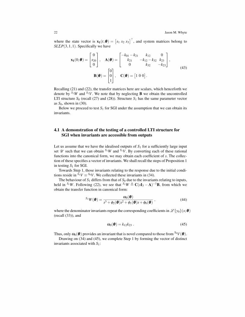
22 Jason M. Whyte
where the state vector is x1(t;θθθ) =[x1 x2 x3
]>, and system matrices belong toSLΣP(3,1,1). Specifically we have
x1(0;θθθ) =
0x200
, A(θθθ) =
−k01− k21 k12 0k21 −k12− k32 k230 k32 −k23
,B(θθθ) =
001
, C(θθθ) =[1 0 0
].
(43)
Recalling (21) and (22), the transfer matrices here are scalars, which henceforth wedenote by S1W and S1V . We note that by neglecting B we obtain the uncontrolledLTI structure S0 (recall (27) and (28)). Structure S1 has the same parameter vectoras S0, shown in (30).
Below we proceed to test S1 for SGI under the assumption that we can obtain itsinvariants.
4.1 A demonstration of the testing of a controlled LTI structure forSGI when invariants are accessible from outputs
Let us assume that we have the idealised outputs of S1 for a sufficiently large inputset U such that we can obtain S1W and S1V . By converting each of these rationalfunctions into the canonical form, we may obtain each coefficient of s. The collec-tion of these specifies a vector of invariants. We shall recall the steps of Proposition 1in testing S1 for SGI.
Towards Step 1, those invariants relating to the response due to the initial condi-tions reside in S1V ≡ S0V . We collected these invariants in (34).
The behaviour of S1 differs from that of S0 due to the invariants relating to inputs,held in S1W . Following (22), we see that S1W , C(sI3−A)−1B, from which weobtain the transfer function in canonical form:
S1W (θθθ) =ω0(θθθ)
s3 +φ2(θθθ)s2 +φ1(θθθ)s+φ0(θθθ), (44)
where the denominator invariants repeat the corresponding coefficients in L {y0}(s;θθθ)(recall (33)), and
ω0(θθθ) = k12k23 . (45)
Thus, only ω0(θθθ) provides an invariant that is novel compared to those from S0V (θθθ).Drawing on (34) and (45), we complete Step 1 by forming the vector of distinct
invariants associated with S1:
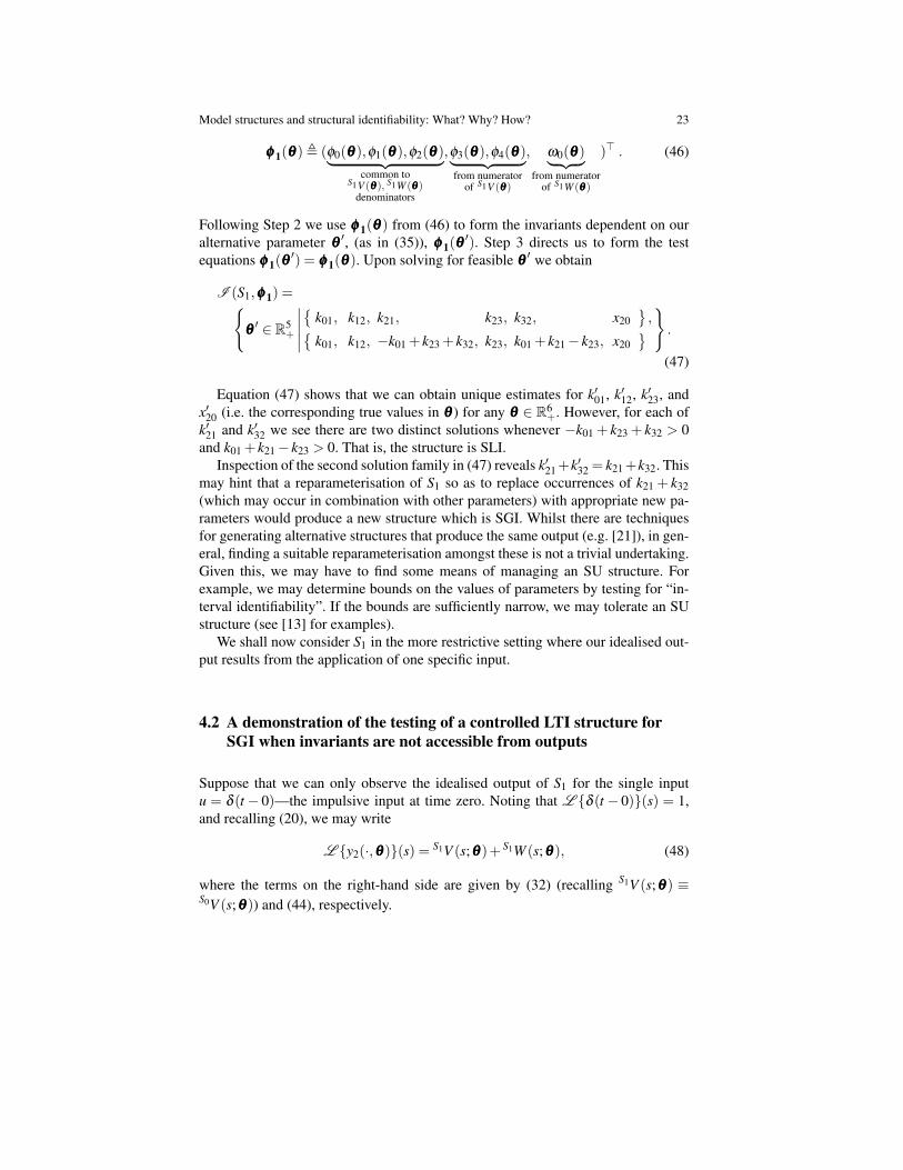
Model structures and structural identifiability: What? Why? How? 23
φφφ 1(θθθ), (φ0(θθθ),φ1(θθθ),φ2(θθθ)︸ ︷︷ ︸common to
S1V (θθθ), S1W (θθθ)denominators
,φ3(θθθ),φ4(θθθ)︸ ︷︷ ︸from numerator
of S1V (θθθ)
, ω0(θθθ)︸ ︷︷ ︸from numerator
of S1W (θθθ)
)> . (46)
Following Step 2 we use φφφ 1(θθθ) from (46) to form the invariants dependent on ouralternative parameter θθθ
′, (as in (35)), φφφ 1(θθθ′). Step 3 directs us to form the test
equations φφφ 1(θθθ′) = φφφ 1(θθθ). Upon solving for feasible θθθ
′ we obtain
I (S1,φφφ 1) ={θθθ′ ∈ R5
+
∣∣∣∣∣{
k01, k12, k21, k23, k32, x20},{
k01, k12, −k01 + k23 + k32, k23, k01 + k21− k23, x20} } .
(47)
Equation (47) shows that we can obtain unique estimates for k′01, k′12, k′23, andx′20 (i.e. the corresponding true values in θθθ ) for any θθθ ∈ R6
+. However, for each ofk′21 and k′32 we see there are two distinct solutions whenever −k01 + k23 + k32 > 0and k01 + k21− k23 > 0. That is, the structure is SLI.
Inspection of the second solution family in (47) reveals k′21+k′32 = k21+k32. Thismay hint that a reparameterisation of S1 so as to replace occurrences of k21 + k32(which may occur in combination with other parameters) with appropriate new pa-rameters would produce a new structure which is SGI. Whilst there are techniquesfor generating alternative structures that produce the same output (e.g. [21]), in gen-eral, finding a suitable reparameterisation amongst these is not a trivial undertaking.Given this, we may have to find some means of managing an SU structure. Forexample, we may determine bounds on the values of parameters by testing for “in-terval identifiability”. If the bounds are sufficiently narrow, we may tolerate an SUstructure (see [13] for examples).
We shall now consider S1 in the more restrictive setting where our idealised out-put results from the application of one specific input.
4.2 A demonstration of the testing of a controlled LTI structure forSGI when invariants are not accessible from outputs
Suppose that we can only observe the idealised output of S1 for the single inputu = δ (t − 0)—the impulsive input at time zero. Noting that L {δ (t − 0)}(s) = 1,and recalling (20), we may write
L {y2(·,θθθ)}(s) = S1V (s;θθθ)+ S1W (s;θθθ), (48)
where the terms on the right-hand side are given by (32) (recalling S1V (s;θθθ) ≡S0V (s;θθθ)) and (44), respectively.
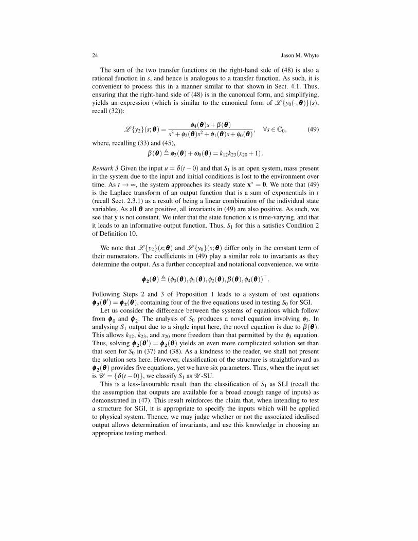
24 Jason M. Whyte
The sum of the two transfer functions on the right-hand side of (48) is also arational function in s, and hence is analogous to a transfer function. As such, it isconvenient to process this in a manner similar to that shown in Sect. 4.1. Thus,ensuring that the right-hand side of (48) is in the canonical form, and simplifying,yields an expression (which is similar to the canonical form of L {y0(·,θθθ)}(s),recall (32)):
L {y2}(s;θθθ) =φ4(θθθ)s+β (θθθ)
s3 +φ2(θθθ)s2 +φ1(θθθ)s+φ0(θθθ), ∀s ∈ C0, (49)
where, recalling (33) and (45),β (θθθ), φ3(θθθ)+ω0(θθθ) = k12k23(x20 +1) .
Remark 3 Given the input u = δ (t−0) and that S1 is an open system, mass presentin the system due to the input and initial conditions is lost to the environment overtime. As t → ∞, the system approaches its steady state x∗ = 0. We note that (49)is the Laplace transform of an output function that is a sum of exponentials in t(recall Sect. 2.3.1) as a result of being a linear combination of the individual statevariables. As all θθθ are positive, all invariants in (49) are also positive. As such, wesee that y is not constant. We infer that the state function x is time-varying, and thatit leads to an informative output function. Thus, S1 for this u satisfies Condition 2of Definition 10.
We note that L {y2}(s;θθθ) and L {y0}(s;θθθ) differ only in the constant term oftheir numerators. The coefficients in (49) play a similar role to invariants as theydetermine the output. As a further conceptual and notational convenience, we write
φφφ 2(θθθ), (φ0(θθθ),φ1(θθθ),φ2(θθθ),β (θθθ),φ4(θθθ))>.
Following Steps 2 and 3 of Proposition 1 leads to a system of test equationsφφφ 2(θθθ
′) = φφφ 2(θθθ), containing four of the five equations used in testing S0 for SGI.Let us consider the difference between the systems of equations which follow
from φφφ 0 and φφφ 2. The analysis of S0 produces a novel equation involving φ3. Inanalysing S1 output due to a single input here, the novel equation is due to β (θθθ).This allows k12, k23, and x20 more freedom than that permitted by the φ3 equation.Thus, solving φφφ 2(θθθ
′) = φφφ 2(θθθ) yields an even more complicated solution set thanthat seen for S0 in (37) and (38). As a kindness to the reader, we shall not presentthe solution sets here. However, classification of the structure is straightforward asφφφ 2(θθθ) provides five equations, yet we have six parameters. Thus, when the input setis U = {δ (t−0)}, we classify S1 as U -SU.
This is a less-favourable result than the classification of S1 as SLI (recall thethe assumption that outputs are available for a broad enough range of inputs) asdemonstrated in (47). This result reinforces the claim that, when intending to testa structure for SGI, it is appropriate to specify the inputs which will be appliedto physical system. Thence, we may judge whether or not the associated idealisedoutput allows determination of invariants, and use this knowledge in choosing anappropriate testing method.

Model structures and structural identifiability: What? Why? How? 25
5 Concluding remarks
This overview has aimed to highlight the benefits of testing model structures for theproperty of structural global identifiability (SGI). Moreover, by assembling crucialdefinitions, drawing important distinctions, and providing test examples, we havesought to illuminate some important concepts in the field of identifiability analysis.We hope that this will encourage and assist interrogation of proposed structures soas to recognise those that are not SGI. This will allow researchers to anticipate thefrustrations almost certain to accompany the use of a non-SGI structure (especially,an unidentifiable one) in modelling and parameter estimation.
Progress in the field of identifiability analysis is ongoing through the develop-ment of new methods of testing structures for SGI or SLI, and refinements to theirimplementation. However, certain practical matters are yet to receive widespreadconsideration. We conclude with brief comments on a selection of these.
Competition—or collaboration—between testing methods? Over a period oftime, the literature has reported that one cannot generally anticipate which methodwill be easiest to apply to a given case, (e.g. [12, Page 96]), or that testing methodsmay suit some problems more than others (e.g. [7]). Consequently, when consid-ering software implementations of testing methods, we may not be able to antici-pate which method will produce a result in the shortest time, or at all. This uncer-tainty has prompted various comparisons aimed at evaluating the utility of alterna-tive methods for testing structures for SGI.
One may wonder if a competitive treatment of methods is a limiting one. That is,might there be benefits in combining methods so as to draw upon their strengths? Forexample, in considering controlled compartmental LTI structures, the TFA providesa means of ascertaining whether or not a structure is generically minimal. If theconclusion is positive, we may then change our approach and apply a suitable testingmethod that uses a type of invariant expected to be simpler than those used in theTFA. For example, we may choose Markov and initial parameters as invariants,expecting these polynomials in the parameters to have a lower degree than thoseseen in transfer function coefficients. Given such simpler invariants, the resultingtest equations will have a reduced algebraic complexity. We could reasonably expectto solve these more quickly than equations obtained from the TFA.
Reproducibility of analysis There is a growing concern over the reproducibilityof studies in computational biology ([16]). We expect a greater awareness of iden-tifiability analysis to encourage the asking of questions that will contribute to arigorous and defensible modelling practice. Beyond this, we may also ponder howto promote reproducibility through the processes by which identifiability analysis isundertaken.
For all but the simplest cases, testing a structure for SGI requires the use of a com-puter algebra system (CAS). Often this is a commercial product, such as MapleTM,Mathematica, or MATLAB. However, as for all complex computer code, one cannotnecessarily guarantee that results produced by a CAS will be correct in all situations(see, for example, [2] noting a limitation of certain versions of MapleTM). As such,

26 Jason M. Whyte
it is good practice for us to check that results obtained from one CAS agree withthose from another.
Performing such a comparison might not be straightforward. Recall that the clas-sical approach to testing a structure for SGI requires the solution of a system ofalgebraic equations. If two CASs employ differing methods in solving a given sys-tem, the solution sets may appear quite dissimilar, even if they are, in fact, the same.This complicates the task of determining whether or not the solution sets are equiv-alent.
We may be able to make choices that can reduce the complexity of the compar-ison problem. One approach is to seek to direct the output of CASs by specifyingsimilar options in their commands where this is possible. For example, the “solve”command in MapleTM allows the user to specify various options, including somerelating to how any solutions are displayed. Another MapleTM option allows somevariables to be specified as “functions of a free variable”. We may be encouragedto use this given the form of solutions obtained from another CAS which we wouldlike to emulate.
The seeming dissimilarity of solutions may be due to features of CAS solutionalgorithms that we cannot directly control. As such, we may seek to manage theseby further scrutinising our equations (or more fundamentally our invariants φφφ(θθθ)),before we attempt to solve them.
Suppose that each (multivariate polynomial) element of φφφ(θθθ) is some combina-tion of simpler polynomials in parameters θθθ . We may determine these new polyno-mials by calculating a Gröbner basis for φφφ(θθθ).7 This requires an “ordering” of pa-rameters, which determines how terms are arranged within a polynomial, and howmonomials are arranged within terms.8 We may obtain differing bases dependingon the chosen ordering.
In certain solution methods (such as “nonlinsolve” in version 1.4 of Python pack-age SymPy) a CAS may (effectively) calculate a Gröbner basis for invariants, choos-ing an ordering without user input. In such cases, should different CASs employdiffering orderings, the solutions of test equations may appear quite different. Assuch, it may be useful for the user to obtain a Gröbner basis for a specified ordering,and use this in formulating test equations for each CAS.
We shall illustrate the importance of the choice of ordering by returning to ourexample structure S1. In Maple 2019 (version 1) we used the “Basis” command(from the “Groebner” package) to compute Gröbner bases for φφφ 1(θθθ) under differ-ent orderings. We varied the ordering of parameters, as specified by the “plex()”option (pure lexicographical ordering). The ordering indicates a decreasing prefer-ence for eliminating parameters from our input polynomials (here, our invariants) aswe proceed from the start of the list, with the aim of forming a “triangular” system
7 We may consider a Gröbner basis for a list of polynomials as analogous to the reduced row-echelon form of a system of linear equations.8 For example, the polynomial x2y+ 2xy3− 4x+ y employs “pure lexicographical ordering” with“x > y”—terms are arranged by decreasing degree of monomials in x, and within each term anymonomial in x appears before one in y. Changing the ordering to “y > x” yields an alternative form:2y3x+ yx2 + y−4x.
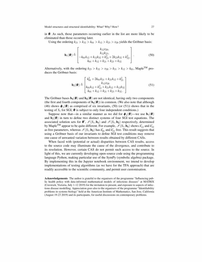
Model structures and structural identifiability: What? Why? How? 27
in θθθ . As such, those parameters occurring earlier in the list are more likely to beeliminated than those occurring later.
Using the ordering k21 > k32 > k01 > k12 > k23 > x20 yields the Gröbner basis:
b1(θθθ),
k12x20,k12k23,
−k01k12 + k12k32 + k223 +2k23k32 + k2
32,k01 + k12 + k21 + k23 + k32
. (50)
Alternatively, with the ordering k23 > k32 > x20 > k21 > k12 > k01, MapleTM pro-duces the Gröbner basis:
b2(θθθ),
k2
01 +2k01k21 + k21k12 + k221
k12x20k01k12 + k2
12 + k21k12 + k12k32k01 + k12 + k21 + k23 + k32 .
(51)
The Gröbner bases b1(θθθ) and b2(θθθ) are not identical, having only two components(the first and fourth components of b1(θθθ)) in common. (We also note that although(46) shows φφφ 1(θθθ) as comprised of six invariants, (50) (or (51)) shows that in thetesting of S1 for SGI, θθθ is subject to only four independent conditions.)
Suppose now that—in a similar manner as we did for φφφ 1(θθθ)—we use b1(θθθ)and b2(θθθ) in turn to define two distinct systems of four SGI test equations. Theassociated solution sets for θθθ
′, I (S1,b1) and I (S1,b2) respectively, determinedby MapleTM appear to be quite different. For example, I (S1,b1) shows k′12 and k′32as free parameters, whereas I (S1,b2) has k′01 and k′21 free. This result suggests thatusing a Gröbner basis of our invariants to define SGI test conditions may removeone cause of unwanted variation between results obtained by different CASs.
When faced with (potential or actual) disparities between CAS results, accessto the source code may illuminate the cause of the divergence, and contribute toits resolution. However, certain CAS do not permit such access to the source. Inlight of this, we are currently developing open-source code using the programminglanguage Python, making particular use of the SymPy (symbolic algebra) package.By implementing this in the Jupyter notebook environment, we intend to developimplementations of testing algorithms (as we have for the TFA approach) that arereadily accessible to the scientific community, and permit user customisation.
Acknowledgements The author is grateful to the organisers of the programme “Influencing pub-lic health policy with data-informed mathematical models of infectious diseases” at MATRIX(Creswick, Victoria, July 1-12 2019) for the invitation to present, and exposure to aspects of infec-tious disease modelling. Appreciation goes also to the organisers of the programme “Identifiabilityproblems in systems biology" held at the American Institute of Mathematics, San Jose, California(August 19-23 2019) and its participants, for useful discussions on contemporary problems.

28 Jason M. Whyte
References
1. American Institute of Mathematics: Identifiability problems in systems biology (2019). URLhttps://aimath.org/workshops/upcoming/identbio/
2. Armando, A., Ballarin, C.: A reconstruction and extension of Maple’s assume facility viaconstraint contextual rewriting. Journal of Symbolic Computation 39, 503–521 (2005)
3. Audoly, S., Bellu, G., D’Angiò, L., Saccomani, M.P., Cobelli, C.: Global identifiability ofnonlinear models of biological systems. IEEE Transactions on Biomedical Engineering 48(1),55–65 (2001)
4. Bellman, R., Åström, K.J.: On structural identifiability. Mathematical Biosciences 7, 329–339(1970). DOI 10.1016/0025-5564(70)90132-X
5. Benvenuti, L., Farina, L.: Minimal positive realizations: a survey of recent results and openproblems. Kybernetika 39(2), 217–228 (2003)
6. Caines, P.E.: Linear Stochastic Systems. John Wiley & Sons, Inc. (1988)7. Chis, O.T., Banga, J.R., Balsa-Canto, E.: Structural identifiability of systems biology models:
a critical comparison of methods. PloS one 6(11), e27755 (2011)8. Cobelli, C., DiStefano III, J.J.: Parameter and structural identifiability concepts and ambigu-
ities: a critical review and analysis. American Journal of Physiology-Regulatory, Integrativeand Comparative Physiology 239(1), R7–R24 (1980). DOI 10.1152/ajpregu.1980.239.1.R7.URL https://doi.org/10.1152/ajpregu.1980.239.1.R7. PMID: 7396041
9. Cox Jr., L.A., Huber, W.A.: Symmetry, Identifiability, and Prediction Uncertainties in Multi-stage Clonal Expansion (MSCE) Models of Carcinogenesis. Risk Analysis: An InternationalJournal 27(6), 1441–1453 (2007)
10. Denis-Vidal, L., Joly-Blanchard, G.: Equivalence and identifiability analysis of uncontrollednonlinear dynamical systems. Automatica 40(2), 287–292 (2004)
11. DiStefano III, J.: Dynamic systems biology modeling and simulation. Academic Press (2015)12. Godfrey, K.: Compartmental Models and Their Application. Academic Press Inc. (1983)13. Godfrey, K., DiStefano III, J.: Identifiability of model parameters. IFAC Proceedings Volumes
18(5), 89–114 (1985)14. van den Hof, J.M.: Structural identifiability from input-output observations. Tech. Rep. BS-
9514, Centrum voor Wiskunde en Informatica, P. O. Box 94079, 1090 GB Amsterdam, TheNetherlands (1995)
15. Jacquez, J.A., Greif, P.: Numerical parameter identifiability and estimability: Integrating iden-tifiability, estimability and optimal sampling design. Mathematical Biosciences 77(1-2), 201–227 (1985)
16. Laubenbacher, R., Hastings, A.: Editorial. Bulletin of Mathematical Biology 80(12), 3069–3070 (2018). DOI 10.1007/s11538-018-0501-8. URL https://doi.org/10.1007/s11538-018-0501-8
17. Poljak, S.: On the gap between the structural controllability of time-varying and time-invariantsystems. IEEE Transactions on Automatic Control 37(12), 1961–1965 (1992)
18. Seber, G.A.F., Wild, C.J.: Nonlinear regression. Wiley series in probability and statistics.Wiley (2003)
19. Vajda, S.: Structural equivalence of linear systems and compartmental models. MathematicalBiosciences 55(1-2), 39–64 (1981)
20. Villaverde, A.F., Barreiro, A., Papachristodoulou, A.: Structural Identifiability of DynamicSystems Biology Models. PLoS Computational Biology 12(10), e1005153 (2016)
21. Walter, E., Lecourtier, Y.: Unidentifiable compartmental models: what to do? Mathematicalbiosciences 56(1-2), 1–25 (1981)
22. Walter, É., Pronzato, L.: Identification of Parametric Models from Experimental Data. Com-munication and Control Engineering. Springer (1997)
23. Whyte, J.M.: On Deterministic Identifiability of Uncontrolled Linear Switching Systems.WSEAS Transactions on Systems 6(5), 1028–1036 (2007)

Model structures and structural identifiability: What? Why? How? 29
24. Whyte, J.M.: A preliminary approach to deterministic identifiability of uncontrolled linearswitching systems. In: 3rd WSEAS International Conference on Mathematical Biology andEcology (MABE’07), Proceedings of the WSEAS International Conferences. Gold Coast,Queensland, Australia (2007)
25. Whyte, J.M.: Inferring global a priori identifiability of optical biosensor experiment mod-els. In: G.Z. Li, X. Hu, S. Kim, H. Ressom, M. Hughes, B. Liu, G. McLachlan, M. Lieb-man, H. Sun (eds.) IEEE International Conference on Bioinformatics and Biomedicine (IEEEBIBM 2013), pp. 17–22. Shanghai, China (2013). DOI 10.1109/BIBM.2013.6732453
26. Whyte, J.M.: Global a priori identifiability of models of flow-cell optical biosensor experi-ments. Ph.D. thesis, School of Mathematics and Statistics, University of Melbourne, Victoria,Australia (2016)
27. Yamada, T., Luenberger, D.G.: Generic Controllability Theorems for Descriptor Systems.IEEE Transactions on Automatic Control AC-30(2), 144–152 (1985)