arX

iv:0

709.

3064

v1 [

cond

-mat

.sup

r-co

n] 1

9 Se

p 20

07

Model for Vortex Pinning in a Two-Dimensional Inhomogeneous

d-Wave Superconductor

Daniel Valdez-Balderas∗ and David Stroud†

Department of Physics, The Ohio State University, Columbus, Ohio 43210

(Dated: February 2, 2008)

Abstract

We study a model for the pinning of vortices in a two-dimensional, inhomogeneous, Type-II

superconductor in its mixed state. The model is based on a Ginzburg-Landau (GL) free energy

functional whose coefficients are determined by the mean field transition temperature Tc0 and

the zero temperature penetration depth λ(0). We find that if (i) Tc0 and λ(0) are functions of

position, and (ii) λ2(0) ∝ Tyc0 with y > 0, then vortices tend to be pinned by regions where Tc0,

and therefore the magnitude of the superconducting order parameter ∆, are large. This behavior

is in contrast to the usual picture of pinning in Type-II superconductors, where pinning occurs in

the small-gap regions. We also compute the local density of states of a model BCS Hamiltonian

with d-wave symmetry, in which the pairing field ∆ is obtained from the Monte Carlo simulations

of a GL free energy. Several features observed in scanning tunneling spectroscopy measurements

on YBa2Cu3O6+x and Bi2Sr2CaCu2O8+x are well reproduced by our model: far from vortex cores,

the local density of states (LDOS) spectra has a small gap and sharp coherence peaks, while near

the vortex cores it has a larger gap with low, broad peaks. Additionally, also in agreement with

experiment, the spectra near the core does not exhibit a zero energy peak which is, however,

observed in other theoretical studies.

∗Electronic address: balderas@mps.ohio-state.edu†Electronic address: stroud@mps.ohio-state.edu

1

I. INTRODUCTION

It is generally believed that vortices in Type II superconductors tend to be pinned in

regions where the gap is small [1]. This is true because a vortex, being a region where the

gradient of the superconducting order parameter is large, locally increases the gradient part

of the free energy. Since this local increase is less in regions where the gap is smaller than

average, the vortex tends to migrate to such regions, according to this picture.

In this paper, we describe a simple model for vortex pinning in an inhomogeneous two-

dimensional (2D) superconductor, in which the vortices tend to be pinned in regions where

the gap is larger than its spatial average. The model is based on a Ginzburg-Landau (GL)

free energy functional in which both the mean-field transition temperature Tc0 and the

zero-temperature penetration depth λ(0) are functions of position, but are correlated in

such a way that regions with large Tc0 also have large λ(0). This assumption seems to

apply to some of the high-Tc cuprate superconductors: according to scanning tunneling

microscopy (STM) experiments on cuprates [2, 3, 4, 5, 6, 7, 8, 9], regions that have a

large gap (proportional to Tc0 in this model) also have a single-particle local density of

states (LDOS) with low, broad peaks, suggestive of a low superfluid density in these regions

[proportional to 1/λ2(0)]. Our model is a generalization of an earlier approach intended to

treat inhomogeneous superconductors in zero magnetic field[10].

In order to further test this vortex pinning model, we also examine the quasiparticle

LDOS near the vortex cores within this model. The proper theoretical description of this

LDOS near the cores is one of the unsolved issues in the field of high-Tc superconductivity.

STM experiments on YBa2Cu3O6+x (YBCO) [11, 12] and Bi2Sr2CaCu2O8+x (Bi2212) [13,

14, 15, 16], show that the local density of states (LDOS) near vortex cores in those materials

has the following characteristics: a dip at zero energy, small peaks at energies smaller than

the superconducting gap, and low, broad peaks at energies above the superconducting gap.

Those features contrast with the spectra shown by conventional superconductors near vortex

cores, where the LDOS usually has a peak at zero energy in clean superconductors (i.e.,

those with a mean-free path larger than the coherence length) [17, 18], or is nearly energy-

independent in dirty superconductors [18, 19].

The zero-energy peak in the LDOS near vortex cores of clean conventional superconduc-

tors can be understood in terms of electronic states with subgap energies bound to vortex

2

cores [20, 21]. However, the structure of the spectra near vortex cores of cuprates is still

lacking an explanation. Several authors have suggested that this structure is due to some

type of competing order which emerges within the vortex cores when superconductivity is

suppressed by a magnetic field [22, 23, 24, 25, 26]. Some of those models, and other de-

scriptions of the spectra near vortex cores, have used the Bogoliubov-de Gennes method

to solve various microscopic Hamiltonians [22, 27, 28, 29, 30, 31], such as BCS-like models

with d-wave symmetry. One recent model for the LDOS near the vortex cores, proposed

by Melikyan and Tesanovic[30], used a Bogoliubov-de Gennes approach to a tight-binding

Hamiltonian. These authors found that, if a homogeneous pairing field is used in the mi-

croscopic Hamiltonian, the LDOS exhibits a zero-energy peak on the atomic sites that are

closest to the vortex cores; this peak is, however, absent from all other sites near the vortex

cores. On the other hand, they found that introducing an enhanced pairing strength for

electrons on nearest-neighbor atomic sites near the vortex cores leads to a suppression of

the zero energy peak, thus obtaining a better agreement with experiment. They speculate

that the enhancement could be due to impurity atoms that pin the vortices, to a distortion

of the atomic lattice by the vortex itself, or to quantum fluctuations of the superconducting

order parameter. The assumption of an enhanced pairing strength is consistent with the

model that we describe in this paper.

In our model, having introduced this correlation between the GL parameters, we anneal

the system to find both the magnitude and the phase of the superconducting order pa-

rameter that minimize the GL free energy at low temperatures. Since the magnetic vector

potential enters the GL free energy functional, this procedure naturally leads to vortex for-

mation. The vortex cores can be identified in our simulations as regions with a large phase

gradient. We find that, in inhomogeneous systems, vortices tend to be pinned in regions

where the superconducting gap is large. For comparison, we also perform a similar annealing

procedure for homogeneous systems. In this case, contrary to inhomogeneous systems, the

magnitude of the superconducting order parameter is reduced near vortex cores. Thus, the

assumption that the gap is large in regions with small superfluid density in inhomogeneous

systems, originally intended to model superconductors in a zero magnetic field [10], leads

naturally to pinning of the vortices in large-gap regions. This approach might therefore be

complementary to that of Ref. [30] mentioned above.

To connect our vortex pinning model to previous studies of the LDOS near vortex cores,

3

we have also studied a microscopic Hamiltonian for electrons on a lattice. This is a tight-

binding model in which electrons on nearest neighbor sites experience a pairing interaction

of the BCS type with d-wave symmetry [10, 32]. The LDOS is obtained by exact numerical

diagonalization of this Hamiltonian. We take the pairing stregth between electrons on near-

est neighbor sites to be proportional to the value of the superconducting order parameter

as determined by the GL simulations using the GL functional just described.

Using this combination of a GL free energy functional and a microscopic d-wave BCS

Hamiltonian, we find that a number of experimental results on cuprates are reproduced well

by our model for inhomogeneous systems. For example, far from vortex cores, the LDOS

shows sharp coherence peaks. Near the vortex cores, our calculated LDOS does not show

a spurious zero energy peak; instead it exhibits a large gap, as well as low, broad peaks

which occur at energies larger than the value of the superconducting energy gap observed

far from vortex cores. Also, in agreement with experiment, the LDOS curves near vortex

cores are similar to those in the large gap regions in systems with quenched disorder but zero

magnetic field[10]); this connection is discussed in section III. One feature not captured by

our model is the existence of small, low energy peaks in the LDOS observed near the vortex

cores.

The rest of the present article is organized as follows. In Section II, we present the

GL free energy functional, as well the microscopic Hamiltonian. In Section III, we present

results for homogeneous and inhomogeneous systems in a magnetic field, as well as results

for inhomogeneous systems in a zero magnetic field for comparison. Finally, in Section IV,

we conclude with a discussion and a summary of our work.

4

II. MODEL

A. Ginzburg-Landau free energy functional

We use a model for a single layer of a cuprate superconductor in a perpendicular magnetic

field based on a GL free energy functional of the form described previously[10]:

F

K1

=

M∑

i=1

(

t

tc0i

+ 3

)

1

λ2i (0)t2c0i

|ψi|2 +

M∑

i=1

1

2(9.38)

1

λ2i (0)t4c0i

|ψi|4

−∑

〈ij〉

2|ψi||ψj |

λi(0)tc0iλj(0)tc0j

cos(θi − θj + A~i~j). (1)

In Eq. (1) the first and second sums are carried over M square cells, each of area equal to

the zero-temperature GL coherence length squared, ξ20 , of a square lattice into which the

superconductor has been discretized for computational purposes. The third sum is carried

out over nearest neighbor cells 〈ij〉. Here

ψi ≡∆i

E0

, (2)

where ∆i is the complex superconducting order parameter of the ith cell, E0 is an arbitrary

energy scale (which we take to be the hopping constant thop ∼ 200 meV)

t ≡kBT

E0

, (3)

is the reduced temperature, T is the temperature, and kB is the Boltzmann constant. Also,

λi(0) is the T = 0 penetration depth and tc0i ≡ kBTc0i/E0, where Tc0i is the mean-field

transition temperature of the ith cell. Therefore, in discretizing the superconductor, we have

assumed that λ(0), Tc0 and ∆ are constant over distances of order ξ0. Finally,

A~i~j =2e

hc

∫ ~j

~i

~A(~r) · d~r (4)

is the integral of the vector potential ~A(~r) from the center of cell i, located at~i, to the center

of cell j, located at ~j, and K1 ≡ h4d/[32(9.38)πm∗2µ2B], where µ2

B ≃ 5.4× 10−5 eV-A3 is the

square of the Bohr magneton, m∗ is twice the mass of a free electron, e is the absolute value

of its charge, and d is the thickness of the superconducting layer. In all of our simulations

we use periodic boundary conditions. A gauge for the magnetic field that allows this is given

in Ref. [10, 33] [see, e. g., eq. (51) of Ref. [10], which gives this gauge choice explicitly for

Nv = 1].

5

We note that the connection between the local superfluid density ns,i(T ) and penetration

depth λi(T ) is such that ns,i(0) ∝ 1/λ2i (0) [10]. Thus, the quantity 1/λ2 in eq. (1) is a way

of describing the local superfluid density, which varies over a length scale of ξ0.

We will be using the above free energy functional at both T = 0 and finite T . Although

we call this a “Ginzburg-Landau free energy functional,” this name is really a misnomer,

since the original GL functional was intended to be applicable only near the mean-field

transition temperature. Strictly speaking, the correct free energy functional near T = 0

should not have the GL form, but would be expected to contain additional terms, such as

higher powers of |ψ|2. We use the GL form for convenience, and because we expect it will

exhibit the qualitative behavior, such as vortex pinning in the large-gap regions, that would

be seen in a more accurate functional.

We assume that the magnetic field is uniform, which is a good approximation for cuprate

superconductors in their mixed state, provided the external field is not too close to the lower

critical field Hc1. In the cuprates, the approximation is satisfactory because the penetration

depth is of the order of thousands of A, while the intervortex distance for the fields we

consider is ∼ 100 A. We employ a gauge that permits periodic boundary conditions, such

that the flux through the lattice can take any integer multiple of hc/e [10, 33]. Thus, the

number Nv of flux quanta hc/(2e) must be an integer multiple of two.

The procedure for choosing the parameters λi(0) and tc0i is similar to that used in Ref. [10].

Basically, in most of the system (α regions), we take λi(0) ∼ λ(0), where λ(0) is the in-

plane penetration depth of a bulk cuprate superconductor [λ(0) ∼ 1800 A in Bi2212, for

example], while tc0i is determined from the typical energy gap in the LDOS as observed in

STM experiments. However, we will also introduce regions (β regions) in which tc0 and λ(0)

are larger than those bulk values. Throughout this article, when we refer to a “gap in the

LDOS,” we mean the distance between the two peaks in the LDOS spectra. This is the

same gap definition used in Ref. [4].

In Ref. [10], we generally introduced inhomogeneities in the superconducting order pa-

rameter ∆i by assuming a binary distribution of tci0, randomly distributed in space: α cells

with a small tci0 and β cells with a large tci0. We also assumed a correlation between λi(0)

and tc0i of the form

λ2i (0) = λ2(0)

(

tc0i

tc0

)y

, (5)

with y = 1. More generally, Eq. (5), with y > 0, accounts for the fact that in STM

6

experiments, regions with a large gap seem to have a small superfluid density (low and

broad peaks.)

In the present article, instead of randomly distributed β cells, we introduce two square

regions with only β cells, while the rest of the lattice is assumed to have only α cells. We

make this choice to study the effects of these inhomogeneities on field-induced vortices. We

also consider a more general model than Ref. [10], allowing y to have values other than only

y = 1.

As shown in Eq. (36) of Ref. [10], in the absence of thermal fluctuations the coupling

constant JXY,ij between cells i and j is approximately

JXY,ij(t) ≃2(9.38)

√

(1 − t/tc0i)(1 − t/tc0j)

λi(0)λj(0)K1. (6)

(The factor of K1 is missing in Ref. [10].) If t << tc0i and t << tc0j, then

JXY,ij(t) ≃2(9.38)K1

λi(0)λj(0). (7)

If we further choose a binary distribution of tc0i, that is,

tc0i =

tc0, if i is on an α cell,

ftc0, if i is on a β cell,(8)

where f is any positive number (typically f > 1), then

JXY,ij(t) ≃2(9.38)K1

λ2(0)·

1 if i and j ∈ α,

1

fy2

if i ∈ α and j ∈ β or if i ∈ β and j ∈ α,

1fy if i and j ∈ β.

(9)

This expression shows that in regions with a large gap the coupling between XY cells is

small, reflecting the large penetration depth in those regions.

B. Microscopic Hamiltonian

Besides using a GL free energy to explore vortex pinning in an inhomogeneous supercon-

ductor, we have also studied the LDOS of a corresponding microscopic model Hamiltonian,

given by [10]:

H = 2∑

〈i,j〉,σ

tijc†iσcjσ + 2

∑

〈i,j〉

(∆ijci↓cj↑ + c.c.) − µ∑

i,σ

c†iσciσ (10)

7

Here∑

〈i,j〉 denotes a sum over distinct pairs of nearest neighbor atomic sites on a square

lattice with N sites, c†jσ creates an electron with spin σ (↑ or ↓) at site j, µ is the chemical

potential, and ∆ij denotes the strength of the pairing interaction between electrons at sites

i and j. Finally, we write tij as

tij = −thop e−iA′

~i~j , (11)

with

A′~i~j

=e

hc

∫ ~j

~i

~A(~r) · d~r. (12)

Here the integral runs along the line from atomic site i, located at ~i, to the atomic site j,

located at ~j, and thop > 0 is the hopping integral for nearest neighbor sites on the lattice.

Note that the prefactor in A′ij involves the factor of hc/e due to a single electronic charge,

and is thus twice as large as that in Aij, which involves the charge of a Cooper pair.

Following Ref. [10] we take ∆ij to be given by

∆ij =1

4

|∆i| + |∆j |

2eiθij , (13)

where

θij =

(θi + θj)/2, if bond 〈i, j〉 is in x-direction,

(θi + θj)/2 + π, if bond 〈i, j〉 is in y-direction,(14)

and

∆j = |∆j|eiθj , (15)

is the value of the complex superconducting order parameter at site j. We will refer to

the lattice over which the sums in (10) are carried out as the atomic lattice (in order to

distinguish it from the XY lattice.) The first term in Eq. (10) thus corresponds to the

kinetic energy, the second term is a BCS type of pairing interaction with d-wave symmetry,

and the third is the energy associated with the chemical potential.

The model we present is similar to the one presented in Ref. [10], the main differences

being the inclusion of a vector potential in the GL free energy functional, and the spatial

distribution of the inhomogeneities. Because the vector potential introduces vortices in the

system, our results differ substantially from our previous work.

8

III. RESULTS

We first present results for homogeneous systems in the presence of an applied transverse

magnetic field equal to two flux quanta through the lattice at low T . This is the lowest

magnetic field consistent with the periodic boundary conditions. In this case, tc0i and

λi(0) are independent of i. Fig. 1 shows our calculated maps of ∆ for a homogeneous

system. In part (a), the lengths and directions of the arrows represent the magnitude and

phase of ∆ in each XY cell. Even though tc0i is homogeneous, the magnetic field renders

∆ inhomogeneous, especially near the vortex cores, where ∆ has a large phase gradient

and a smaller magnitude. This behavior is familiar from Ginzburg-Landau treatments of

homogeneous Type II superconductors in a magnetic field. Part (b) of Fig. 1 shows a map

of |∆|, with dark (light) regions representing small (large) value of |∆|. The vortex cores

are the darkest regions.

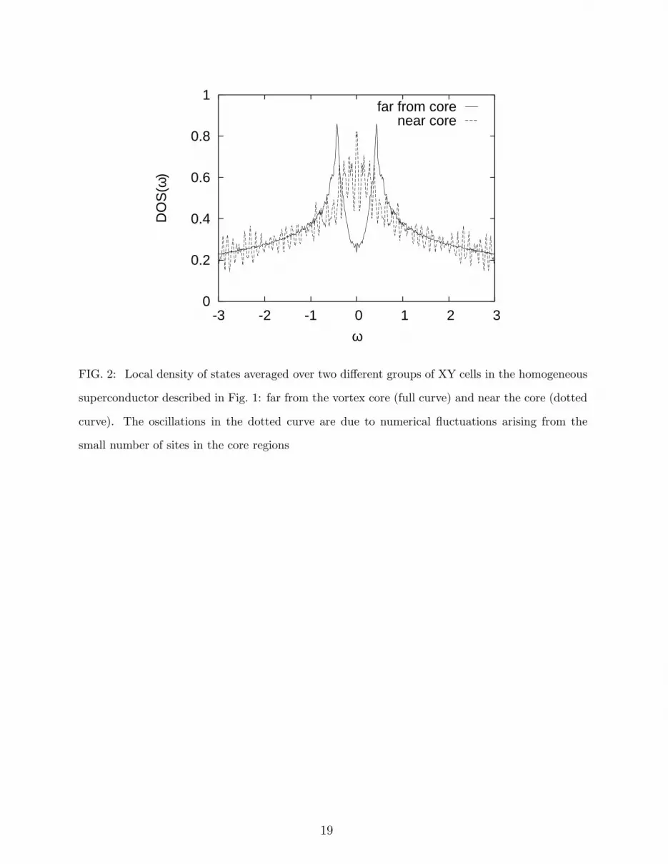
Fig. 2 show the LDOS averaged over regions near and far from the vortex cores of the

system described in Fig. 1. Since |∆| is small near the core, we have defined an XY cell to

be “near the core” if |∆| ≤ |∆avg|/2 in that cell, where |∆avg| is the value of |∆| averaged

over all the XY cells of the lattice. All other cells are considered to be far from the core.

Thus, in order to compute the averaged quantities shown in Fig. 2, we first calculated the

LDOS on every atomic site by exact numerical diagonalization of the Hamiltonian (10),

and then averaged the LDOS over the the set of atomic sites near and far from the vortex

cores, as defined above. We have chosen to enclose nine atomic sites inside each XY cell for

this system, because the coherence length in cuprates is ∼ 15 A, approximately three times

larger than the atomic lattice constant, ∼ 5 A.

Fig. 2 shows that, in a homogeneous system, the LDOS far from the core is strongly

suppressed near ω = 0, and exhibits sharp coherence peaks, reminiscent of a d-wave super-

conductor in the absence of a magnetic field. Near the vortex cores, on the other hand,

the gap is filled, and the LDOS is large near ω = 0, resembling the spectrum of a gapless

tight-binding model in two dimensions and zero magnetic field [10, 34]. The spectrum near

the core has considerable numerical noise, because it represents an average over only a few

atomic sites. In particular, the rapid oscillations are probably due to this numerical artifact.

To estimate our magnetic fields, we note that, because of the numerical implementation

of the periodic boundary conditions [10, 35], the field has to be chosen so that the number

9

Nv of magnetic flux quanta Φ0 = hc/(2e) through the system is a multiple of two. Therefore,

the magnetic field can be estimated using B = NvΦ0/S where S is the area of the system,

and Φ0 ≡ hc/(2e) ≈ 2×10−15 T-m2. In the present article we use a numerical sample of area

area S = (48a0)2, where a0 ∼ 5 A is the atomic lattice constant. Therefore B ≈ Nv × 3 T,

and for the systems containing two vortices, B ∼ 6T. The magnitude of this magnetic field

is comparable used in STM experiments[13, 14].

We now briefly discuss the temperature evolution of 〈|∆|2〉, defined as an average of

〈|∆i|2〉 over all XY lattice cells i, for systems with homogeneous tc0 in a transverse magnetic

field. Here, 〈...〉 denotes a thermal average, obtained using Monte Carlo simulations. Fig. 3

shows curves of 〈|∆|2〉(t) versus reduced temperature t, for systems of the same size subject

to different magnetic fields, and therefore containing different numbers of vortices Nv. In

the zero magnetic field case, Nv = 0, 〈|∆|2〉(t) has a minimum as a function of t, which

occurs near the phase ordering temperature. Fig. 3 shows that, as the field is increased, the

phase ordering temperature is reduced, and around Nv = 36, it seems to drop to zero. The

fact that of 〈|∆|2〉(t) increases with t for large t is an artifact of the GL functional, as has

been discussed in detail in [10] for the case B = 0.

We now proceed to show systems with inhomogeneities. Fig. 4 shows gap maps of systems

in which tc0i, and therefore JXY,ij, are are i dependent. Specifically, two square regions, of

size 4×4 XY cells each, have tc0i = ftc0, with f = 3; those are called β cells, as described

in the previous section. The remainder of the XY cells have tc0i = tc0, and are called α

cells. Clearly, the vortices are pinned in the β regions, where |∆| is large. The fact that |∆|

is large in β regions is of course due to the fact that at low temperatures, |∆| is roughly

proportional to tc0. On the other hand, in order to understand why the vortices are pinned

in the large-|∆| regions, we note that JXY,ij at low temperatures can be estimated with the

use of eq. (9). For the particular parameters used in this calculation, namely, x = 3 and

f = 3, JXY,ij is about 27 times smaller within β regions than in the α regions. Because

of this ratio, phase gradients near the vortex cores cost much less energy in the β regions

than in the α regions, even though |∆| is larger in the β regions. Thus, it is energetically

favorable for the vortices to be pinned in the β regions.

Fig. 5 shows the LDOS averaged over α and β regions of the system shown in Fig. 4.

This Figure shows that, far from the vortex cores (α regions), the LDOS is very similar

to that of regions far from the core in homogeneous system at low magnetic field [cf. Fig.

10

2] - both spectra have a small gap and sharp coherence peaks. However, in contrast to

the homogeneous case, the LDOS of the inhomogeneous system exhibits a large gap and

broadened peaks near the vortex core. This LDOS spectrum is similar to that calculated

for the large gap regions of systems with quenched disorder and no magnetic field in our

previous work [10]. In the present case, the gap in the LDOS is large in the β regions, of

course, because of the large value of tc0i and therefore of |∆|, near the vortex cores. The

peaks in the LDOS in the β region above the gap are low and broad, on the other hand,

because of the large phase gradient of the superconducting order parameter in these regions.

It is as if the system has lost phase coherence in those regions due to the presence of the

vortex core. We can more clearly see this point by comparing the LDOS of a β region

containing a pinned vortex core to that of a β region in a system in a zero magnetic field,

in which, therefore, there is no vortex core to be pinned. We now describe this system.

Fig. 6 shows a system at low temperature with two inhomogeneities, similar to that shown

in Fig. 4, but with zero rather than a finite magnetic field. Clearly, in the ground state, as

expected, the phase of ∆ is almost uniform. Furthermore, and also as expected, |∆| is larger

in the β regions, which have a larger value of tc0i. However, when we turn to the LDOS

(Fig. 7), the LDOS of the β regions is characterized by much sharper coherence peaks than

that at finite magnetic field described in the previous paragraph, presumably because of the

absence of a large phase gradient.

We have also tested the sensitivity of our results to lattice size and to the number of

atomic sites per XY cell. To do this, we performed calculations similar to the ones described

above, but with 24×24 instead of 16×16 XY lattices, each XY cell containing four instead of

nine atomic lattice sites. Fig. 8 shows the results for a 24×24 XY lattice of an inhomogeneous

system in the presence of a magnetic field. As in the 16×16 case, the vortices are pinned

in the regions with large ∆ and small JXY,ij. Fig. 9 shows that the LDOS for this system

both near and far from the core is nearly the same as that of the 16×16 system shown in

Fig. 5. Likewise, a system with 24×24 XY cells and two atomic sites per XY cell, but with

no magnetic field, is shown in Fig. 10; the corresponding LDOS averaged over regions near

and far from the core is shown in Fig. 11. The LDOS shown in this Figure has the same

features as that of the 16×16 system shown in Fig. 7. We thus conclude that our results are

not very sensitive to the lattice sizes used, nor to the number of atomic sites per XY cell.

In the calculations described above, have assumed that λ2 ∝ T yc0. If y ≥ 3, then the

11

vortices are consistently pinned in the large gap region. By contrast, if y = 1, we find the

vortices may or may not be pinned in the large gap region, depending on where these regions

are located within the computational lattice. The vortices obviously go to the large gap

region because of the correlation between λ2 and Tc0. As mentioned earlier, this correlation

originates in the fact large λ2 implies a small energy cost to introduce a gradient in the

phase of the order parameter. Such a gradient must exist near a vortex core; therefore, the

vortex prefers to be in a region where this gradient is energetically inexpensive. Melikyan

and Tesanovic [30] discuss various other possible causes of larger pinning in the large gap

region; these include quantum fluctuations, distortion of the atomic lattice by the vortices,

and the pinning of vortices by impurity atoms. Our model could be viewed as a special

kind of such impurity pinning, in which the “impurities” are superconducting regions with

a large gap and large penetration depth. We have also looked at how the size of the pinning

regions affects the pinning. The pinning is generally more effective for large pinning regions,

probably because the vortex energy is reduced by a larger amount if pinned in a region of

large pinning area, all other parameters being the same.

Finally, we note the similarity between our calculated LDOS versus energy curves for

regions near the vortex cores, and the corresponding curves for large gap regions of inhomo-

geneous systems with quenched disorder in a zero magnetic field, calculated in our previous

work [10]. Those similarities have been implied in several experimental papers. For example,

Lang et al.[4] discussed the similarity between the spectra of large-gap regions of inhomo-

geneous systems at low temperatures in a zero field and those observed in the pseudogap

regime of some cuprate superconductors. In the pseudogap region, the phase configuration

is disordered and therefore, possibly like the β region at zero field, both might be consid-

ered as “normal” regions. Likewise, Fischer et al. [36] have also noted the similarity of the

low-T spectra near the vortex cores to spectra in the pseudogap regime. Once again, the

similarity may arise because both the interior of the vortex cores and the pseudogap region

may be considered as “normal”. Thus, both of these reports implicitly suggest a similarity

between the low-T spectra in the large gap regions of a disordered system at B = 0 and the

corresponding spectra near vortex cores at finite B.

12

IV. DISCUSSION

We have presented a model for the pinning of vortices by inhomogeneities in a two-

dimensional type II superconductor at low temperatures. The model is based on a GL

free energy functional, and it is inspired by our previous study [10] of the LDOS in an

inhomogeneous superconductor in zero magnetic field. In our model, we have proposed a

GL free energy functional in which regions with a large value of the superconducting order

parameter have a large penetration depth, as suggested by zero-field STM experiments on

cuprates. Using an annealing process and Monte Carlo simulations, we have found that the

pinning of vortices by those large-gap regions emerges naturally from the functional form

of our GL free energy. The vortices are attracted to the large-gap regions, in our model,

because the large penetration depth leads to a small coupling between cells in those regions.

Therefore, the phase of the superconducting order parameter can more easily bend in these

regions, and this in turn allows the large-gap regions to accomodate a vortex more easily

than regions with a small gap. By contrast, in the absence of quenched inhomogeneities,

minimization of the GL free energy functional yields a spatial configuration in which the

superconducting order parameter is suppressed near vortex cores.

It is worth commenting further on the qualitative physics underlying the pinning of the

vortices in the region of enhanced local Tc. Basically, this pinning behavior occurs because, in

our model, a locally enhanced Tc corresponds to a locally suppressed superfluid density. This

superfluid density is proportional to the local 1/λ2, and is related to the Ginzburg-Landau

coefficients, as we have described earlier. The vortices can be more easily accommodated

in these large-Tc regions because the large phase gradients which characterize the vortices

cost less energy in such regions. Although we describe the pinning in terms of the variation

of 1/λ2, the pinning is not due to any kind of “magnetic” forces - the quantity 1/λ2 is

just a way of describing the local superfluid density. Thus, just as in conventional pinning,

the vortices are attracted to regions of lower free energy. The major difference is that the

superfluid density (and 1/λ2) is proportional to Tc in the present model, rather than being

independent of, or inversely correlated with Tc as in more conventional pinning. This leads

to pinning in a large-Tc region rather than a small-Tc region. We also emphasize that,

although our pinning results are obtained using rather elaborate numerical calculations, the

underlying physics is straightforward: the pinning behavior is consistent with qualitative

13

expectations, given the model.

It may seem strange to consider the spatial variation in 1/λ2 as occurring over a scale

of ξ0 ∼ 15A, when λ itself is of order 103 A or more. However, it should be remembered

that 1/λ2 is related to the coefficients of the Ginzburg-Landau free energy [see eq. (1)],

and these coefficients are, in fact, expected to vary over a scale of ξ0. Thus, the model

is, indeed, reasonable and consistent with the expected physics. It is the local superfluid

density (proportional to 1/λ2) which varies over a scale of ξ0.

It is also worth commenting on what kind of real systems could be described by our

model. Even if one neglects the weak Josephson coupling between the layers of a high-

Tc material, there will still be magnetic interactions between pancake vortices in adjacent

layers, so that the system will not be truly 2D. Likewise, if we wish to use this model to

describe a very thin 2D high-Tc film, there are stray fields in vacuum extending into the third

dimension, which will contribute to the total energy. In both cases, our model is definitely an

oversimplification. Nonetheless, our model does seem to describe some observed features in

real high-Tc materials, suggesting that it captures some significant physics in these systems.

Thus, we consider our model as a possible starting point for a fully realistic treatment of

either 3D high-Tc materials or very thin 2D high-Tc layers.

We have connected our work on the pinning of vortices to continuing efforts by several

groups to describe the density of states near vortices in cuprates superconductors. To do this,

we have studied a model BCS Hamiltonian with d-wave symmetry, in which the pairing field

is obtained from simulations of the GL free energy functional. We use exact diagonalization

to compute the local density of states on each atomic site of the lattice described by this

Hamiltonian. For homogeneous systems, we found that the LDOS near the vortex cores

resembles that of a gapless tight-binding model in two dimensions, with a Van Hove peak at

zero energy. However, when we introduce the inhomogeneities with a large pairing field and

large penetration depth that pin the vortices, the LDOS near the vortex cores is markedly

different from that of the homogeneous systems. Namely, this LDOS exhibits a large gap

as well as low and broadened peaks at energies greater than that of the superconducting

gap fa.r from the vortex core. Also, our calculated LDOS near the vortex cores in this

inhomogeneous case does not exhibit the spurious zero-energy peak which is present in

several other theoretical studies but is absent from experiments. All of these features in our

calculations are consistent with results observed in STM experiments on YBCO [11, 12] and

14

Bi2212 [13, 14, 15, 16].

Our results are also consistent with those obtained of Ref. [30], using a somewhat different

model. Those authors obtain better agreement between their calculated LDOS spectra and

experiment[14], if they assume an enhanced rather than uniform pairing field near the vortex

cores. In particular, introducing this large pairing field near the vortex core in their model

suppresses the unphysical zero-energy peak. Our approach, in which a large gap is correlated

with a large penetration depth, may heop justify the occurrence of this larger pairing field

in the vortex cores.

Finally, we briefly comment on the possible physical origin of correlation between large

gap and large penetration depth. The origin of the spatial fluctuations of Tc0 observed in

the cuprates may be the local fluctuations in concentration, which are highly likely since the

cuprates are mostly disordered alloys and the local concentration would involve an average

a coherence length, which is only about 15 A . But Tc0 is proportional to the gap (i.

e., presumably, the pseudogap), which increases with decreasing concentration of charge

carriers, whereas 1/λ2(0) is proportional to the superfluid density, which should decrease

with decreasing charge carrier concentration. Therefore, we expect Tc0 to be positively

correlated with λ2(0), as seen experimentally and as used in the present model.

V. ACKNOWLEDGMENTS

This work was supported by NSF grant DMR04-13395. The computations described here

were carried out through a grant of computing time from the Ohio Supercomputer Center.

We thank Prof. J. Orenstein for a useful conversation about the origin of the correlation

between superconducting gap and penetration depth.

[1] G. Blatter, M. V. Feigel’man, V. B. Geshkenbein, A. I. Larkin, and V. M. Vinokur, Rev. Mod.

Phys.66, 1125 2000.

[2] T. Cren, D. Roditchev, W. Sacks, J. Klein, J.-B. Moussy, C. Deville-Cavellin, and M. Lagues,

Phys. Rev. Lett. 84, 147 (2000).

[3] C. Howald, P. Fournier, and A. Kapitulnik, Phys. Rev. B 64, 100504(R) (2001).

15

[4] K. M. Lang, V. Madhavan, J. E. Hoffman, E. W. Hudson, H. Eisaki, S. Uchida, and J. C.

Davis, Nature 415, 412 (2002).

[5] C. Howald, H. Eisaki, N. Kaneko, M. Greven, and A. Kapitulnik, Phys. Rev. B 67, 014533

(2003).

[6] T. Kato, S. Okitsu, and H. Sakata, Phys. Rev. B 72, 144518 (2005).

[7] A. C. Fang, L. Capriotti, D. J. Scalapino, S. A. Kivelson, N. Kaneko, M. Greven, and A. Ka-

pitulnik, Phys. Rev. Lett. 96, 017007 (2006).

[8] H. Mashima, N. Fukuo, Y. Matsumoto, G. Kinoda, T. Kondo, H. Ikuta, T. Hitosugi, and

T. Hasegawa, Phys. Rev. B 73, 060502(R) (2006).

[9] S. H. Pan, J. P. O’Neal, R. L. Badzey, C. Chamon, H. Ding, J. R. Engelbrecht, Z. Wang,

H. Eisaki, S. Uchida, A. K. Gupta, et al., Nature 413, 282 (2001).

[10] D. Valdez-Balderas and D. Stroud, Phys. Rev. B 74, 174506 (2006).

[11] I. Maggio-Aprile, C. Renner, A. Erb, E. Walker, and O. Fischer, Phys. Rev. Lett. 75, 2754

(1995).

[12] C. Renner, B. Revaz, K. Kadowaki, I. Maggio-Aprile, and O. Fischer, Phys. Rev. Lett. 80,

3606 (1998).

[13] G. Levy, M. Kugler, A. A. Manuel, O. Fischer, M. Li, Phys. Rev. Lett. 95, 257005 (2005).

[14] S. H. Pan, E. W. Hudson, A. K. Gupta, K.-W. Ng, H. Eisaki, S. Uchida, and J. C. Davis,

Phys. Rev. Lett. 85, 1536 (2000).

[15] K. Matsuba, H. Sakata, N. Kosugi, H. Nishimori, and N. Nishida, Journal of the Physical

Society of Japan 72, 2153 (2003).

[16] B. Hoogenboom, C. Renner, B. Revaz, I. Maggio-Aprile, and O. Fischer, Physica C 332, 440

(2000).

[17] H. F. Hess, R. B. Robinson, and J. V. Waszczak, Phys. Rev. Lett. 64, 2711 (1990).

[18] C. Renner, A. D. Kent, P. Niedermann, O. Fischer, and F. Levy, Phys. Rev. Lett. 67, 1650

(1991).

[19] Y. De Wilde, M. Iavarone, U. Welp, V. Metlushko, A. E. Koshelev, I. Aranson, G. W. Crabtree,

and P. C. Canfield, Phys. Rev. Lett. 78, 4273 (1997).

[20] C. Caroli, P. G. D. Gennes, and J. Matricon, Physics Letters 9, 307 (1964).

[21] J. D. Shore, M. Huang, A. T. Dorsey, and J. P. Sethna, Phys. Rev. Lett. 62, 3089 (1989).

[22] M. Franz and Z. Tesanovic, Phys. Rev. Lett. 80, 4763 (1998).

16

[23] D. P. Arovas, A. J. Berlinsky, C. Kallin, and S.-C. Zhang, Phys. Rev. Lett. 79, 2871 (1997).

[24] M. Franz and Z. Tesanovic, Phys. Rev. B 63, 064516 (2001).

[25] J. H. Han and D.-H. Lee, Phys. Rev. Lett. 85, 1100 (2000).

[26] J.-i. Kishine, P. A. Lee, and X.-G. Wen, Phys. Rev. B 65, 064526 (2002).

[27] P. I. Soininen, C. Kallin, and A. J. Berlinsky, Phys. Rev. B 50, 13883 (1994).

[28] Y. Wang and A. H. MacDonald, Phys. Rev. B 52, R3876 (1995).

[29] J.-X. Zhu and C. S. Ting, Phys. Rev. Lett. 87, 147002 (2001).

[30] A. Melikyan and Z. Tesanovic, Physical Review B 74, 144501 (2006).

[31] O. Vafek, A. Melikyan, M. Franz, and Z. Tesanovic, Phys. Rev. B 63, 134509 (2001).

[32] T. Eckl, D. J. Scalapino, E. Arrigoni, and W. Hanke, Phys. Rev. B 66, 140510(R) (2002).

[33] W. Yu, K. H. Lee, and D. Stroud, Phys. Rev. B 47, 5906 (1993).

[34] F. F. Assaad, Phys. Rev. B 65, 115104 (2002).

[35] W. Yu, K. H. Lee, and D. Stroud, Phys. Rev. B 47, 5906 (1993).

[36] O. Fischer, M. Kugler, I. Maggio-Aprile, C. Berthod, and C. Renner, Rev. Mod. Phys. 79,

353 (2007).

[37] E. Bittner and W. Janke, Phys. Rev. Lett. 89, 130201 (2002).

17

HaL HbL

FIG. 1: Map of the pairing field ∆ over a homogeneous, two-dimensional superconductor of

area 16ξ0 × 16ξ0 in a transverse, uniform magnetic field B ≃ 6T. The superconductor has been

discretized into XY cells, each of which has an area ξ20 and encloses nine atomic sites. In part (a)

the length and direction of each arrow represents the complex value of ∆ within an XY cell. Part

(b) shows a map of the magnitude |∆| of the pairing field. Dark (light) regions represent a small

(large) value of |∆|. Vortex cores can be easily identified as the darkest regions.

18

0

0.2

0.4

0.6

0.8

1

-3 -2 -1 0 1 2 3

DO

S(ω

)

ω

far from corenear core

FIG. 2: Local density of states averaged over two different groups of XY cells in the homogeneous

superconductor described in Fig. 1: far from the vortex core (full curve) and near the core (dotted

curve). The oscillations in the dotted curve are due to numerical fluctuations arising from the

small number of sites in the core regions

19

0

0.02

0.04

0.06

0.08

0.1

0.12

0.14

0.16

0.18

0 0.01 0.02 0.03 0.04 0.05 0.06 0.07 0.08

<|∆

|2 >

t

Nv=0Nv=2Nv=4Nv=6

Nv=12Nv=18Nv=24Nv=30Nv=36Nv=42Nv=54

FIG. 3: Thermal average 〈|∆|2〉 of the squared magnitude of the superconducting order parameter

versus the reduced temperature t for a system with a homogeneous tc0 placed in various fields. The

magnitude of the magnetic field is B ≃ Nv × 3T as described in the text. We can observe that the

minimum of 〈|∆|2〉(t) versus t (which is known to occur near the phase ordering temperature in

zero magnetic field systems [10, 37]) is shifted toward smaller values of t with increasing magnetic

field.

20

HaL HbL

FIG. 4: Map of the pairing field ∆ in an inhomogeneous, two-dimensional superconductor of area

16ξ0×16ξ0 in a transverse, uniform magnetic field B ≃ 6 T. The superconductor has two β regions

where tc0i is large; these correspond to the light regions in (b). The system has been discretized

into XY cells, each of which has an area ξ20 and encloses nine atomic sites. In part (a) each arrow

represents the complex value of ∆ within an XY cell. Part (b) shows a map of the magnitude |∆|

of the pairing field. Dark (light) regions represent a small (large) value of |∆|. The locations of

the two vortex cores can be identified as the regions with a large phase gradient in part (a). They

are pinned to regions with a large |∆| because of the low value of the coupling between XY cells

in those regions. The present results are obtained from Eqs. (8) and (9), using f = 3 and x = 3.

21

0

0.2

0.4

0.6

0.8

1

-4 -3 -2 -1 0 1 2 3 4

DO

S(ω

)

ω

αβ

FIG. 5: Local density of states averaged over two different groups of XY cells in the inhomogeneous

superconductor shown in Fig. 4: far from the core (α) and near the core (β). In agreement with

experimental results, this Figure shows that (i) far from vortex cores the LDOS shows sharp

coherence peaks; (ii) near the vortex cores, the LDOS does not display the unphysical zero-energy

peak obtained in other models. Instead (iii), it has a large gap, as well as low and broad peaks.

HaL HbL

FIG. 6: Same as Fig. 4, but for a system at B = 0 instead of B 6= 0. At low temperatures, the

phase of ∆ is almost uniform, since, in the absence of a magnetic field, phase gradients cost energy.

As expected, ∆ is larger in the β regions, which have a large value of tc0i.

22

0

0.2

0.4

0.6

0.8

1

1.2

-4 -3 -2 -1 0 1 2 3 4

DO

S(ω

)

ω

αβ

FIG. 7: Local density of states for the system shown in Fig. 6. The LDOS in the β regions of this

system has much sharper peaks than the LDOS of the β regions for the corresponding system in a

finite magnetic field shown in Fig. 5. This result shows that having a large gap is not a sufficient

condition to observe broadened peaks near vortex cores; a large phase gradient is also required.

HaL HbL

FIG. 8: Similar to Fig. 4, but the system has 24×24 instead of 16×16 XY cells, each with four

instead of nine atomic lattice sites.

23

0

0.2

0.4

0.6

0.8

1

-4 -3 -2 -1 0 1 2 3 4

DO

S(ω

)

ω

αβ

FIG. 9: Local density of states averaged over regions far from the vortex cores, for the system

shown Fig. 8. Results are very similar to the corresponding system with 16×16 cells, which has

nine instead of four atoms per XY cell, and is shown in Fig. 5. Thus, our results are not strongly

dependent on the size of the XY cell or of the XY lattice.

HaL HbL

FIG. 10: Same as Fig. 6 but for a system consisting of 24×24 instead of 16×16 XY cells, each

having four instead of nine atomic sites.

24

0

0.2

0.4

0.6

0.8

1

1.2

-4 -3 -2 -1 0 1 2 3 4

DO

S(ω

)

ω

αβ

FIG. 11: Same as Fig. 7 but for a system of 24×24 instead of 16×16 XY cells, each having cell

has four rather than the nine atomic sites.

25