microlensing of circumstellar envelopes. iii. line profiles from stellar winds in homologous...

arX

iv:a

stro

-ph/

0511

551v

1 1

8 N

ov 2

005

Astronomy & Astrophysics manuscript no. windlens February 5, 2008(DOI: will be inserted by hand later)

Microlensing of Circumstellar Envelopes

III. Line profiles from stellar winds in homologous expansion

M. A. Hendry1,2, R. Ignace2,3, and H. M. Bryce1,3

1 Department of Physics and Astronomy, University of Glasgow, G12 8QQ, UK2 Department of Physics, Astronomy and Geology, Box 70652, East Tennessee State University,

Johnson City, Tennessee, 37614, USA3 Department of Astronomy, University of Wisconsin, 475 North Charter Street, Madison, Wisconsin,

53706, USA

Received ...; Accepted ...

Abstract. This paper examines line profile evolution due to the linear expansion of circumstellarmaterial obsverved during a microlensing event. This work extends our previous papers on emissionline profile evolution from radial and azimuthal flow during point mass lens events and fold causticcrossings. Both “flavours” of microlensing were shown to provide effective diagnostics of bulk motionin circumstellar envelopes. In this work a different genre of flow is studied, namely linear homologousexpansion, for both point mass lenses and fold caustic crossings. Linear expansion is of particularrelevance to the effects of microlensing on supernovae at cosmological distances. We derive line profilesand equivalent widths for the illustrative cases of pure resonance and pure recombination lines, modelledunder the Sobolev approximation. The efficacy of microlensing as a diagnostic probe of the stellarenvirons is demonstrated and discussed.

Key words. Line: profiles – Stars: circumstellar matter – Supernovae: general – Gravitational lensing

1. Introduction

Recently gravitational microlensing has been shownto be a powerful tool for probing not only the natureand distribution of dark matter but also the astro-physical properties of the source being lensed (see,for example, Gould 2001 for a comprehensive review).While the vast majority of microlensing events ob-served to date can be adequately approximated aspoint sources lensed by a point mass lens, there is asmall but significant fraction of events in which thesource must be modelled as extended , which has im-portant consequences for the evolution of the broad-band lightcurve and spectrum during the microlens-ing event and produces observational signatures thatare now readily detectable – chiefly due to the intro-duction of microlensing ‘alert’ networks. This devel-opment has allowed intensive photometric and spec-troscopic monitoring of many microlensing events,

Send offprint requests to: M.A.. Hendry

spearheaded by the PLANET collaboration (Albrowet al. 1998). The alert strategy is especially well-suited to fold caustic crossings – in e.g. close binarylensing events – since observation of the first caus-tic crossing permits prediction of the second causticcrossing, allowing intensive follow-up observations tobe scheduled. Moreover, every fold caustic crossingmust be treated as an extended source event, makingthem ideal probes of the astrophysics of the source.

In the past few years ‘alert response’ broad-band pho-tometric observations of extended source microlens-ing events have shown clear detections of stellar limbdarkening on the photospheres of a number of stars,including: K giants (Albrow et al. 1999; Albrow etal. 2000; Fields et al 2003), a metal-poor A dwarfin the Small Magellanic Cloud (Afonso et al. 2000),a G/K subgiant (Albrow et al. 2001a) and an F8-G2 solar-type star (Abe et al. 2003). These observa-tions have been used to estimate limb darkening pa-rameters and to constrain stellar atmosphere models,

http://arXiv.org/abs/astro-ph/0511551v1

2 M. A. Hendry et al.: Microlensing of stellar winds in homologous expansion

comparing for example the LTE ATLAS models ofKurucz (1994) with the PHOENIX ‘Next Generation’models of Hauschildt et al. (1999).

In addition Albrow et al. (2001b) used the VLT tocarry out observations of Hα equivalent width varia-tion in the atmosphere a K3 bulge giant during a foldcaustic crossing event. These authors showed thathighly resolved observations of the microlensed spec-trum could be a powerful discriminant between differ-ent stellar atmosphere models, and indeed could alsobe a useful method for breaking the near-degeneracybetween the parameters of different lens models. Thiswork essentially vindicated the theoretical modellingof Heyrovsky, Sasselov and Loeb (2000), which pre-dicted that with 8m-class telescopes it should be pos-sible to use highly time- and spectrally-resolved ob-servations of microlensing events to carry out ‘tomog-raphy’ of stellar atmospheres.

A notable feature of the theoretical literature onextended source microlensing events, however, hasbeen the comparative neglect of extended circum-

stellar envelopes. Although the model developed inColeman (1998) and Simmons et al. (2002) includessuch a scattering envelope, and Coleman et al. (1997)also considered the case of a non-spherical envelope(e.g., a Be disk), these computations were carried outonly for the broad-band photometric and polarimet-ric response to a microlensing event.

In two preceding papers, Ignace & Hendry (1999) andBryce, Ignace and Hendry (2003) calculated the mi-crolensing signatures of emission line profiles fromexpanding and rotating spherical shells, lensed by apoint mass lens and a fold caustic respectively. Theirresults were for highly simplistic velocity fields – con-stant expansion or constant rotation – in order to iso-late the effects of the microlensing and demonstrateclearly the diagnostic potential for deriving velocityinformation about the shells. The authors showedthat, while in the absence of lensing the integratedline profiles for expanding and rotating shells yieldedidentical ‘flat top’ profiles in each case, microlensingclearly breaks the degeneracy between these cases.

In this third paper, we choose to focus on the par-ticular case of circumstellar media in homologous ex-pansion, with radial velocity v(r) ∝ r. This case isinteresting for two reasons. Firstly, this type of veloc-ity law applies to the early phases of nova and super-nova (SN) explosions. Since the latter are observed tocosmological distances, it becomes increasingly likelythat such events will be lensed as the light from theSN makes its way from a distant galaxy to the Earth(c.f. Dalal et al. 2003). Thus a consideration of ho-mologous expansion is relevant if only to investigatedefinite signatures of microlensing from emission pro-

file shapes observed in SN events. Indeed Bagherpouret al. (2004) consider the microlensed lightcurves ofType Ia SN, and Bagherpour et al. (2005) extendtheir analysis to consider the impact of microlensingon P Cygni profiles in the spectra of Type Ia SN.Secondly, in this paper we employ standard Sobolevtheory to model the emission line profiles; the Sobolevapproximation is valid for the highly supersonicflows commonly found in SNe and stellar winds.Furthermore the case of homologous expansion leadsto a significant simplification of the expressions anda consequent substantial reduction in computationaleffort. Thus it is worthwhile studying this case to bet-ter appreciate the characteristics of how microlensingwill affect emission lines formed in winds with moregeneral velocity laws.The structure of this paper is as follows. In Section 2we describe the basic features of line formation the-ory, and the Sobolev approximation which we employ.In Section 3 we derive, and briefly discuss, unlensedprofiles for the case of pure resonance and pure re-combination lines, in a stellar wind undergoing ho-mogolous expansion. In Section 4 we present illus-trative results, calculating the time evolution of lineprofile and equivalent width for pure resonance andpure recombination lines lensed by a point mass lensand a fold caustic. Finally in Section 5 we discuss ourresults and their future applicability in a number ofspecific astrophysical contexts.

2. Line formation theory

We first need to derive the emission profile for theunlensed case, expressed in terms of intensity as afunction of frequency and position within the enve-lope of circumstellar material. For an envelope in bulkmotion such that the flow speed greatly exceeds thethermal broadening, the locus of points contributingto the emission at any particular frequency in theline profile is confined to an “isovelocity zone” (c.f.,Mihalas 1978). These zones are determined by theDoppler shift formula, namely

νz = ν0

(

1 − vz

c

)

, (1)

where the observer’s coordinates are (x, y, z) with theline-of-sight along z, νz is the Doppler shifted fre-quency, and vz = −v(r) · z is the projection of theflow velocity onto the line-of-sight (as indicated inFigures 1 and 2). Note that both Cartesian (x, y, z)and spherical (r, ϑ, ϕ) coordinates can be defined forthe star. Employing the Sobolev theory for line pro-file calculation in moving media reduces the radia-tion transfer in a moving envelope to a calculation

M. A. Hendry et al.: Microlensing of stellar winds in homologous expansion 3

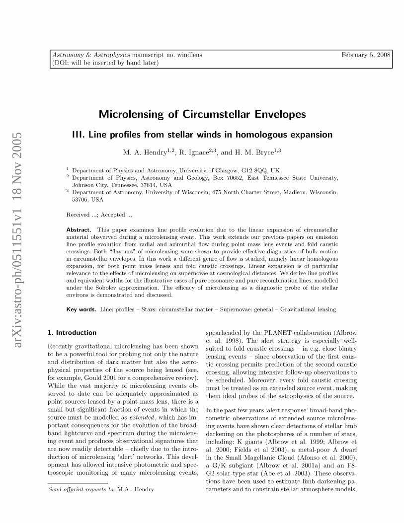
Fig. 1. A schematic showing the contribution from dif-ferent regions to the line profile shape, for an observeron the right hand side. Much of the line emission is pro-duced around the circular tube indicated in projection bythe dashed lines. On the far side (left hand side) of thetube the emission will be occulted by the star. On thenear side, the circumstellar material will attenuate thecontinuum emission from the central photosphere.

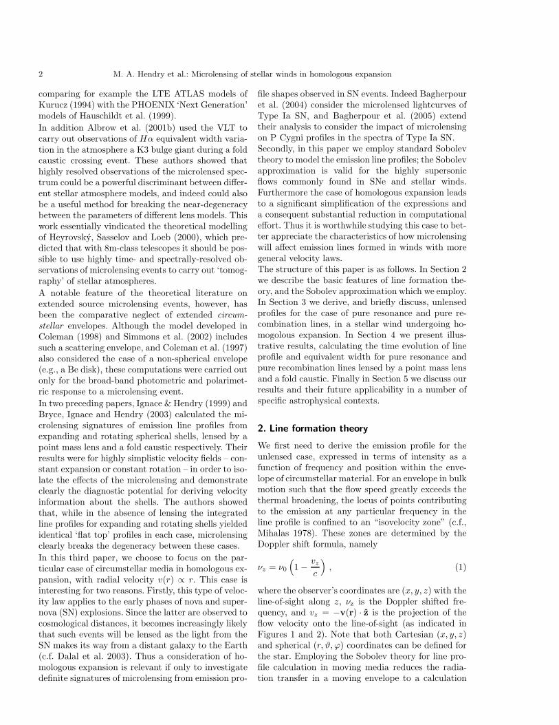
Fig. 2. A schematic showing the isovelocity zones (sur-faces of constant vz) for our velocity model. These arecircular plane surfaces which are oriented normal to theobserver’s line-of-sight. We assume that the photosphereis of radius R, and the envelope is of maximum radialextent rmax.

in which one need consider only distinct isovelocityzones. Equation (1) will therefore prove crucial forrelating the variable profile shape to the kinematicsof the envelope.For the assumed linear expansion, and for an enve-lope of maximum radial extent rmax, the velocity v

at radial distance r is given by

v = vmax (r/rmax) r , (2)

where r is a unit vector in the radial direction andvmax is the wind speed at r = rmax. The velocityshift as seen by the observer, situated as in Figure 1,is then

vz = −vmax(r/rmax) cosϑ = −vmax (z/rmax) , (3)

where ϑ is the angle between the radial direction andthe line of sight.Thus isovelocity zones for constant vz are seen to beplane surfaces. In fact, given the spherical symmetryof our model, the isovelocity zones are circular planesurfaces of radius

pmax =√

r2max − z2 , (4)

as depicted in Figure 2.Consider a projected element of the stellar wind atfixed impact parameter p, and angle α measuredclockwise from x – i.e. x = p cosα and y = p sin α.The emergent intensity Iν(p)1 due to emission fromthe wind is given by

Iν(p) =

∫ ∞

z

κν(r) ρ(r)Sν e−τν dz′ , (5)

where κν is the opacity, ρ the density, Sν the sourcefunction, and τν the optical depth at radial distancer, satisfying r2 = p2 + z′2.The Sobolev approximation is to evaluate the opticaldepth only at the point where the Doppler shiftedfrequency of a gas parcel exactly equals the observedfrequency. This delta function response in frequencysimplifies considerably the expression for the opticaldepth, namely

τν(z) =

∫ ∞

z

κν(r) ρ(r) δ(νz − νz′) dz′

=κν(r) ρ(r)λ0

|dvz/dz|z. (6)

The denominator on the right hand side is the line-of-sight velocity gradient. For a spherical flow, thisgradient is given by the expression

dvz

dz= µ2 dv

dr+ (1 − µ2)

v

r. (7)

For the case of homologous expansion, with v(r) =vmax (r/rmax), the line-of-sight velocity gradient sim-plifies to dvz/dz = vmax/rmax, which is a con-stant. Therefore, although the Sobolev optical depthwill generally depend on angle ϑ through the factordvz/dz, homologous expansion is the single exceptionfor which the optical depth depends on radius only.The optical depth is now

τν(r) =κν(r) ρ(r)λ0 rmax

vmax. (8)

1 Note that the spherical symmetry of our model meansthat the emergent intensity is independent of α.


Knowing the optical depth as a function of r, we canthen obtain an expression for the intensity, Iν(p), us-ing equations (4) and (6) and the equation

p2 = r2 − z2 . (9)

In Sobolev theory the intensity then reduces to theform

Iν(p) = Sν(r)(

1 − e−τν(r))

. (10)

Allowing for line emission from resonance line scat-tering and collisional de-excitation, and defining ǫ asthe ratio of the collisional de-excitation rate to thatof spontaneous decay, the source function can be de-rived to be

Sν =βc I∗,ν + ǫ Bν

β + ǫ. (11)

The two parameters βc and β are respectively thepenetration and escape probabilities, which are givenby

βc =1

4π

∫

Ω∗

1 − e−τν

τν

dΩ , (12)

and

β =1

4π

∫

4π

1 − e−τν

τν

dΩ , (13)

where Ω∗ is the solid angle subtended by the star atradius r.

The optical depth is generally anisotropic, but as al-ready noted for homologous expansion the opticaldepth is isotropic in this special case. As a result,the penetration and escape probabilities are easilycalculable, and in particular βc = W (r)β, where thedilution factor

W (r) = 0.5 (1 −√

1 − R2/r2) . (14)

So for linear expansion, we have the well-knownresult that the Sobolev optical depth is a function ofradius only. Since the source function also dependsonly on radius (or equivalently on impact parameter,p, at fixed vz), so too does the intensity. To computethe total emergent flux at a given Doppler shift inthe line profile due to emission in the circumstellarenvelope, we must integrate over emergent intensitybeams as given by

Fν(vz) =1

D2

∫

vz

Iν(p) p dp dα , (15)

where D is the distance from the Earth. Substitutingin for the intensity, the integration for the flux be-comes

Fν(vz) =2π

D2

∫ pmax

pmin

Sν(r)(

1 − e−τν(r))

p dp . (16)

where we have, of course, performed the (trivial) inte-gral over the angle α, and the limits pmin and pmax arediscussed below. For homologous expansion we knowthat the Sobolev surfaces are disks oriented trans-verse to the line-of-sight (i.e., with z = constant).From equation (9) this means that pdp = rdr, andso the above flux integral could be equivalently re-formulated as

Fν(vz) =2π

D2

∫ rmax

rmin

Sν(r)(

1 − e−τν(r))

r dr . (17)

We now include the contribution of continuum ra-diation from a pseudo-photosphere at radius R. Itis instructive to consider separately redshifted andblueshifted wavelengths, which correspond to vz > 0and v(z) < 0 respectively.For v(z) > 0 (the redshifted side) the total fluxFtot(vz) at frequency ν and line-of-sight velocity vz

may be written as

Ftot(vz) = F1(vz) + F2(vz) , (18)

where

F1(vz) =2π

D2

∫ R

0

Iphot p dp , (19)

and

F2(vz) =2π

D2

∫ pmax

R

Sν(r)(

1 − e−τν(r))

p dp . (20)

Here Iphot is the continuum intensity of the pseudo-photosphere. If Iphot is a constant then the integralsinvolving Iphot become very straightforward. F1 rep-resents the flux coming directly from the pseudo-photosphere while F2 accounts for photons scatteredby the surrounding envelope which emerge along theline of sight. Note that the lower limit of the F2 in-tegral is R since the region for p < R is occulted bythe pseudo-photosphere of the star. The upper limit,pmax satisfies the relation

p2max = r2

max − z2 . (21)

For v(z) < 0 (the blueshifted side) the total flux con-sists of three terms, i.e.

Ftot(vz) = F3(vz) + F4(vz) + F5(vz) , (22)


where

F3(vz) =2π

D2

∫ plim

0

Iphot p dp , (23)

F4(vz) =2π

D2

∫ pmax

plim

Sν(r)(

1 − e−τν(r))

p dp , (24)

and

F5(vz) =2π

D2

∫ R

plim

Iphot e−τν(r) p dp . (25)

Here plim is defined as

plim =

√R2 − z2 for 0 ≤ z ≤ R

0 for z > R. (26)

Note that if z > R then the F3 integral is identi-cally zero; in this case the flux contribution fromthe pseudo-photosphere is represented fully by theF5 term, which also takes account of attenuation byintervening wind material along the line-of-sight.Finally we must stress that, in accordance with thestandard notation adopted in the microlensing liter-ature, all distance scales are in fact taken as angulardistances that are normalised to the angular Einsteinradius of the lens. This implies that the “fluxes”defined in the above equations have rather unusualunits. however, the results of our line profile calcu-lations in the following sections will be displayed asratios normalised by the continuum, so that the (non-standard) units of flux will cancel.

3. Unlensed profiles from homologous

expansion

Before including the effects of gravitational lensingwe first consider the unlensed profiles derived by ap-plying the model of the previous section to the il-lustrative cases of a pure resonance line and a purerecombination line. We have computed line profilesfor a range of optical depths, assuming a sphericallysymmetric density distribution for the ejecta givenby

ρ(x) = ρ0 x−3 , (27)

where x = r/R. The factor x−3 accounts for masscontinuity within the shell as material expands. Thescale parameter ρ0 denotes the density at the ra-dius of the pseudo-photosphere and specifies the totalamount of gas ejected in the explosion, via the equa-tion

Mejecta =

∫

4πr2 ρ(r) dr . (28)

3.1. Pure resonance lines

For the case of a pure resonance line the parameterǫ is set to zero in eq. (11), and the source functionbecomes

Sν = W (r) I∗,ν . (29)

The opacity for resonance line scattering does notdepend explicitly on density, but an implicit depen-dence can arise through, for example, the ionizationfraction of whatever atomic species is being consid-ered. For simplicity, we suppress any radial depen-dence of the opacity in our model, and parametrizethe Sobolev optical depth as

τν = τ0 (ρ/ρ0) = τ0 x−3 . (30)

An especially convenient parameter used to charac-terize different line calculations is the line integratedoptical depth defined as follows

T =

∫ xmax

1

τν dx =1

2τ0

(

1 − 1

x2max

)

. (31)

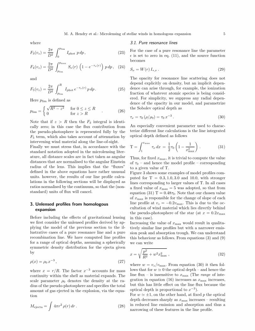
Thus, for fixed xmax, it is trivial to compute the valueof τ0 – and hence the model profile – correspondingto a given value of T.Figure 3 shows some examples of model profiles com-puted for T = 0.3, 1.0, 3.0 and 10.0, with strongerlines corresponding to larger values of T. In all casesa fixed value of xmax = 5 was adopted, so that fromequation (31) T = 0.48τ0. Note that our chosen valueof xmax is responsible for the change of slope of eachline profile at vz = −0.2vmax. This is due to the oc-cultation of wind material which lies directly behindthe pseudo-photosphere of the star (at x = 0.2xmax

in this case).Increasing the value of xmax would result in qualita-tively similar line profiles but with a narrower emis-sion peak and absorption trough. We can understandthis behaviour as follows. From equations (3) and (9)we can write

x =

√

p2

R2+ w2x2

max , (32)

where w = vz/vmax. From equation (30) it then fol-lows that for w ≃ 0 the optical depth – and hence theline flux – is insensitive to xmax (The range of inte-gration in equation (16) increases as xmax increases,but this has little effect on the line flux because theoptical depth is proportional to x−3).For w ≃ ±1, on the other hand, at fixed p the opticaldepth decreases sharply as xmax increases – resultingin reduced line emission and absorption and thus anarrowing of these features in the line profile.


3.2. Pure recombination lines

We have also computed model profiles for the caseof a pure recombination line. As such, scattering isignored, and the source function is assumed to arisefrom an LTE process, so that

Sν = Bν(T ) , (33)

for temperature, T . For simplicity, the envelope shallbe taken as isothermal. The opacity for a recombina-tion line is κ ∝ ρ, and so the scaling of the opticaldepth will for this case be

τν = τ0 (ρ/ρ0)2. (34)

As a ρ2 process, the optical depth will go as x−6 – astrong function of radius.It is again useful to introduce the integrated opticaldepth parameter given by

T =

∫ xmax

1

τ0 (ρ/ρ0)2 dx , (35)

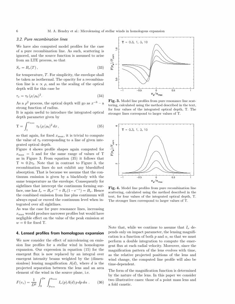
so that again, for fixed xmax, it is trivial to computethe value of τ0 corresponding to a line of given inte-grated optical depth.Figure 4 shows profile shapes again computed forxmax = 5 and for the same range of values of Tas in Figure 3. From equation (35) it follows thatT ≈ 0.2τ0. Note that in contrast to Figure 3, therecombination lines do not exhibit any blueshiftedabsorption. That is because we assume that the con-tinuum emission is given by a blackbody with thesame temperature as the envelope. Consequently forsightlines that intercept the continuum forming sur-face, one has Iν = Bνe−τ +Bν(1−e−τ) = Bν . Hencethe combined emission from line plus continuum willalways equal or exceed the continuum level when in-tegrated over all sightlines.As was the case for pure resonance lines, increasingxmax would produce narrower profiles but would havenegligible effect on the value of the peak emission atw = 0 for fixed T.

4. Lensed profiles from homologous expansion

We now consider the effect of microlensing on emis-sion line profiles for a stellar wind in homologousexpansion. Our expression in equation (15) for theemergent flux is now replaced by an integral overemergent intensity beams weighted by the (dimen-sionless) lensing magnification A(d), where d is theprojected separation between the lens and an areaelement of the wind in the source plane, i.e.

F (vz) =1

D2

∫ 2π

0

∫ pmax

pmin

Iν(p)A(d) p dp dα . (36)

Fig. 3. Model line profiles from pure resonance line scat-tering, calculated using the method described in the text,for four values of the integrated optical depth, T. Thestronger lines correspond to larger values of T.

Fig. 4. Model line profiles from pure recombination linescattering, calculated using the method described in thetext, for four values of the integrated optical depth, T.The stronger lines correspond to larger values of T.

Note that, while we continue to assume that Iν de-pends only on impact parameter, the lensing magnifi-cation is a function of both p and α, so that we mustperform a double integration to compute the emer-gent flux at each radial velocity. Moreover, since themagnification pattern of the lens evolves with time,as the relative projected positions of the lens andwind change, the computed line profile will also betime-dependent.

The form of the magnification function is determinedby the nature of the lens. In this paper we considertwo illustrative cases: those of a point mass lens anda fold caustic.


4.1. Point mass lensing event

In the typical microlensing situation of a point masslens the (time-dependent) magnification factor takesthe well-known form (see e.g. Pacynski 1986)

A(u) =u2 + 2

u√

u2 + 4(37)

where u is the impact parameter : the projected sep-aration between the lens and source element, givenby

u(t) =

√

u20 +

(t − t0)2

t2E(38)

where t0 is the time of closest approach between lensand source element, which occurs at u = u0, the min-imum impact parameter, and tE is the characteristictimescale of the event. Both u and u0 are expressedin units of the angular Einstein radius of the lens,which is defined as

θE =

√

4GM

c2

DS − DL

DSDL

(39)

where M , DS , DL are the lens mass, source distanceand lens distance respectively. The timescale tE maybe written as

tE =θE

µrel(40)

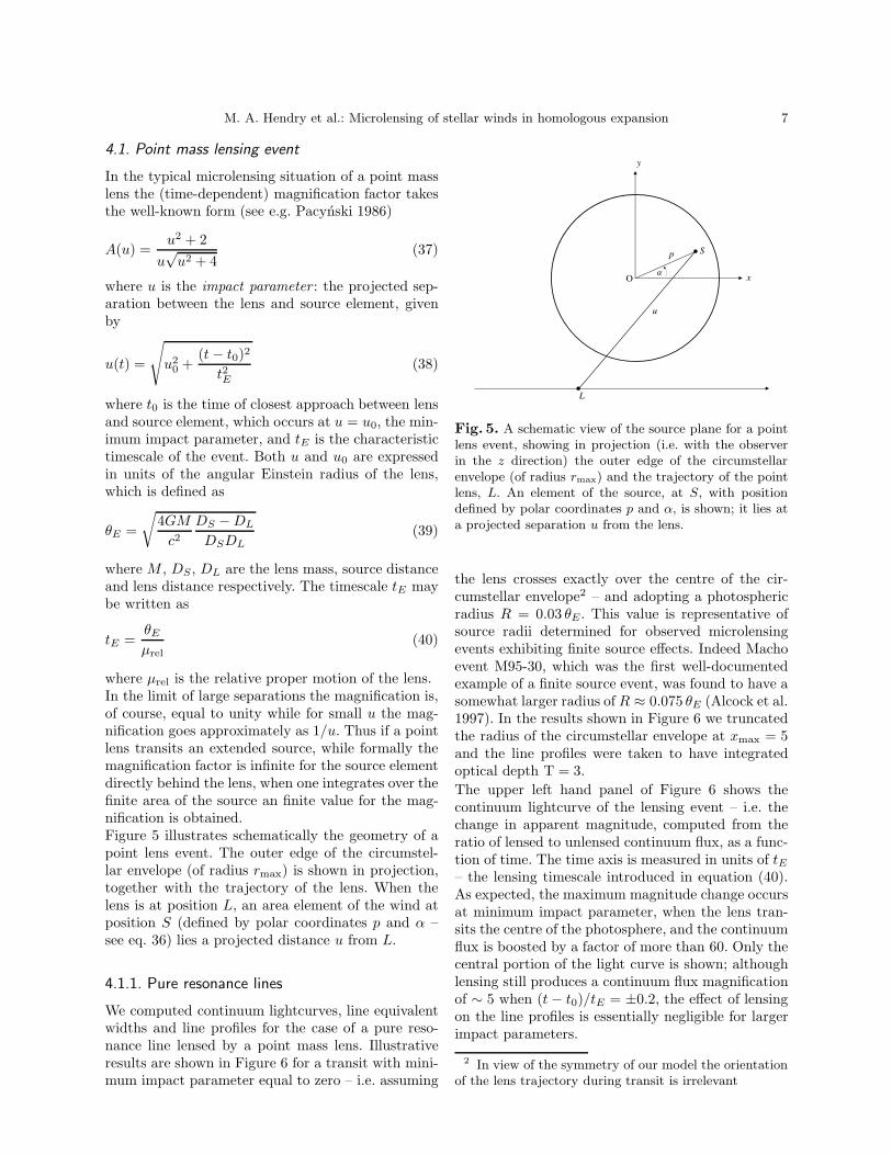
where µrel is the relative proper motion of the lens.In the limit of large separations the magnification is,of course, equal to unity while for small u the mag-nification goes approximately as 1/u. Thus if a pointlens transits an extended source, while formally themagnification factor is infinite for the source elementdirectly behind the lens, when one integrates over thefinite area of the source an finite value for the mag-nification is obtained.Figure 5 illustrates schematically the geometry of apoint lens event. The outer edge of the circumstel-lar envelope (of radius rmax) is shown in projection,together with the trajectory of the lens. When thelens is at position L, an area element of the wind atposition S (defined by polar coordinates p and α –see eq. 36) lies a projected distance u from L.

4.1.1. Pure resonance lines

We computed continuum lightcurves, line equivalentwidths and line profiles for the case of a pure reso-nance line lensed by a point mass lens. Illustrativeresults are shown in Figure 6 for a transit with mini-mum impact parameter equal to zero – i.e. assuming

y

L

u

O

p S

x

Fig. 5. A schematic view of the source plane for a pointlens event, showing in projection (i.e. with the observerin the z direction) the outer edge of the circumstellarenvelope (of radius rmax) and the trajectory of the pointlens, L. An element of the source, at S, with positiondefined by polar coordinates p and α, is shown; it lies ata projected separation u from the lens.

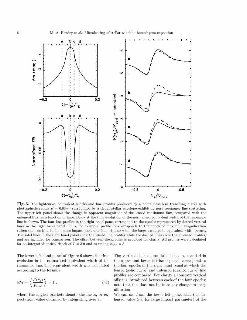
the lens crosses exactly over the centre of the cir-cumstellar envelope2 – and adopting a photosphericradius R = 0.03 θE. This value is representative ofsource radii determined for observed microlensingevents exhibiting finite source effects. Indeed Machoevent M95-30, which was the first well-documentedexample of a finite source event, was found to have asomewhat larger radius of R ≈ 0.075 θE (Alcock et al.1997). In the results shown in Figure 6 we truncatedthe radius of the circumstellar envelope at xmax = 5and the line profiles were taken to have integratedoptical depth T = 3.

The upper left hand panel of Figure 6 shows thecontinuum lightcurve of the lensing event – i.e. thechange in apparent magnitude, computed from theratio of lensed to unlensed continuum flux, as a func-tion of time. The time axis is measured in units of tE– the lensing timescale introduced in equation (40).As expected, the maximum magnitude change occursat minimum impact parameter, when the lens tran-sits the centre of the photosphere, and the continuumflux is boosted by a factor of more than 60. Only thecentral portion of the light curve is shown; althoughlensing still produces a continuum flux magnificationof ∼ 5 when (t − t0)/tE = ±0.2, the effect of lensingon the line profiles is essentially negligible for largerimpact parameters.

2 In view of the symmetry of our model the orientationof the lens trajectory during transit is irrelevant


Fig. 6. The lightcurve, equivalent widths and line profiles produced by a point mass lens transiting a star withphotospheric radius R = 0.03 θE surrounded by a circumstellar envelope exhibiting pure resonance line scattering.The upper left panel shows the change in apparent magnitude of the lensed continuum flux, compared with theunlensed flux, as a function of time. Below it the time evolutioin of the normalised equivalent width of the resonanceline is shown. The four line profiles in the right hand panel correspond to the epochs represented by dotted verticallines in the right hand panel. Thus, for example, profile ‘b’ corresponds to the epoch of maximum magnification(when the lens is at its minimum impact parameter) and is also when the largest change in equivalent width occurs.The solid lines in the right hand panel show the lensed line profiles while the dashed lines show the unlensed profiles,and are included for comparison. The offset between the profiles is provided for clarity. All profiles were calculatedfor an integrated optical depth of T = 3.0 and assuming xmax = 5.

The lower left hand panel of Figure 6 shows the timeevolution in the normalised equivalent width of theresonance line. The equivalent width was calculatedaccording to the formula

EW =

⟨

F (vz)

Fcont

⟩

− 1 , (41)

where the angled brackets denote the mean, or ex-pectation, value obtained by integrating over vz.

The vertical dashed lines labelled a, b, c and d inthe upper and lower left hand panels correspond tothe four epochs in the right hand panel at which thelensed (solid curve) and unlensed (dashed curve) lineprofiles are compared. For clarity a constant verticaloffset is introduced between each of the four epochs;note that this does not indicate any change in mag-nification.We can see from the lower left panel that the un-lensed value (i.e. for large impact parameter) of the


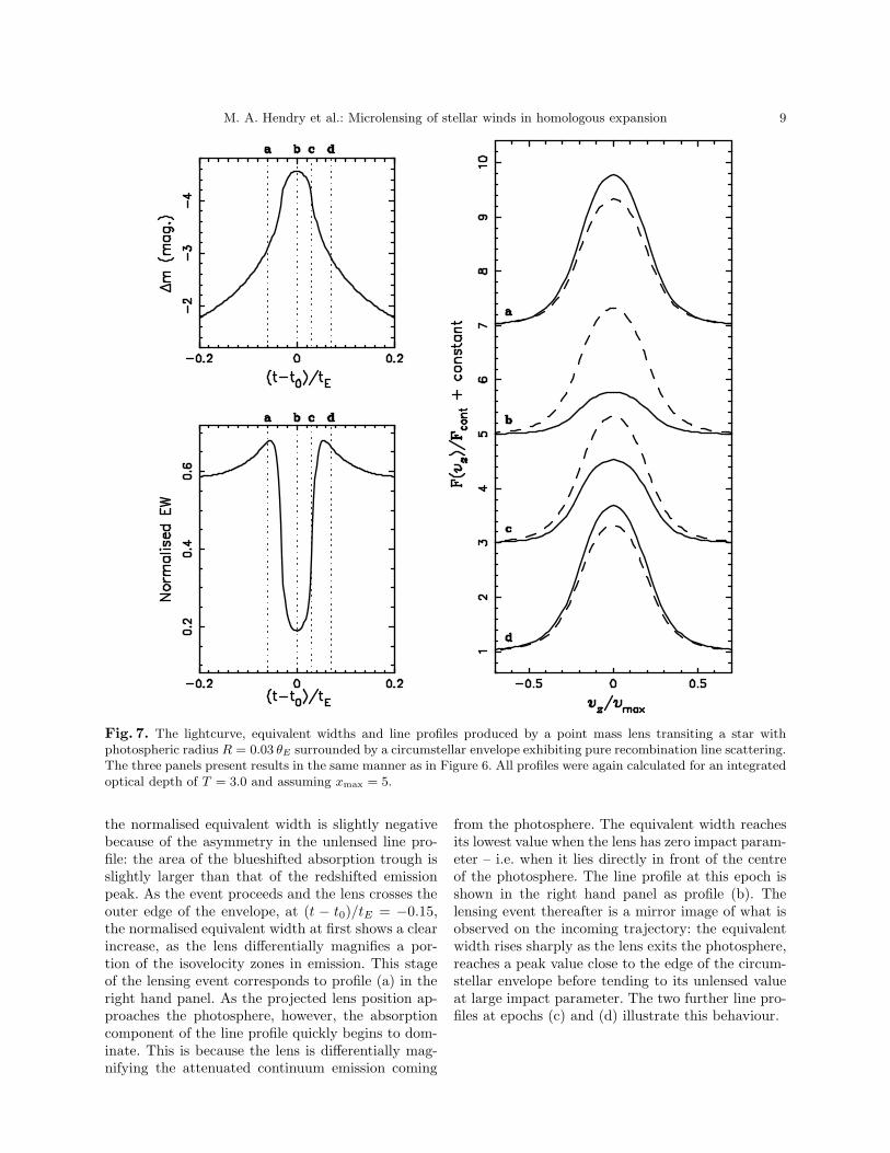
Fig. 7. The lightcurve, equivalent widths and line profiles produced by a point mass lens transiting a star withphotospheric radius R = 0.03 θE surrounded by a circumstellar envelope exhibiting pure recombination line scattering.The three panels present results in the same manner as in Figure 6. All profiles were again calculated for an integratedoptical depth of T = 3.0 and assuming xmax = 5.

the normalised equivalent width is slightly negativebecause of the asymmetry in the unlensed line pro-file: the area of the blueshifted absorption trough isslightly larger than that of the redshifted emissionpeak. As the event proceeds and the lens crosses theouter edge of the envelope, at (t − t0)/tE = −0.15,the normalised equivalent width at first shows a clearincrease, as the lens differentially magnifies a por-tion of the isovelocity zones in emission. This stageof the lensing event corresponds to profile (a) in theright hand panel. As the projected lens position ap-proaches the photosphere, however, the absorptioncomponent of the line profile quickly begins to dom-inate. This is because the lens is differentially mag-nifying the attenuated continuum emission coming

from the photosphere. The equivalent width reachesits lowest value when the lens has zero impact param-eter – i.e. when it lies directly in front of the centreof the photosphere. The line profile at this epoch isshown in the right hand panel as profile (b). Thelensing event thereafter is a mirror image of what isobserved on the incoming trajectory: the equivalentwidth rises sharply as the lens exits the photosphere,reaches a peak value close to the edge of the circum-stellar envelope before tending to its unlensed valueat large impact parameter. The two further line pro-files at epochs (c) and (d) illustrate this behaviour.


4.1.2. Pure recombination lines

We also computed continuum lightcurves, equivalentwidths and line profiles for the case of a pure recom-bination line lensed by a point mass lens. Illustrativeresults are shown in Figure 7 for exactly the samewind and lens parameters as in Figure 6.

The upper left panel of Figure 7 is, of course, identicalto that of Figure 6, since it shows the magnification ofthe continuum flux. The time evolution of the equiva-lent width also shows qualitatively similar behaviourto that of the resonance line case, although the mag-nitude of the maximum change in equivalent widthis approximately five times larger; this is essentiallydue to the stronger dependence of the optical depthon radius for a recombination line.

Again we see that the equivalent width first increasesas the lens transits the circumstellar envelope, dueto the differential magnification of the emission fluxfrom the region around the star. When the lens tran-sits the photosphere, on the other hand, the differen-tial magnification of the attenuated continuum fluxfrom the photosphere again causes a sharp decrease inequivalent width, which reaches its minimum value atzero impact parameter. The symmetry of the isove-locity zones and the lens trajectory then results insymmetric behaviour during the second half of theevent.

4.2. Fold caustic lensing event

For a binary lensing event the magnification patternin the source plane is, in general, a rather compli-cated function of the lens masses and separations. Aswe remarked in Section 4.1, for a single point lens themagnification A(u) goes as 1/u as u → 0, so that themagnification is formally infinite at only one point– coincident with the position of the point lens it-self, for which u = 0. For a binary lens, on the otherhand, the magnification is formally infinite along oneor more closed curves, or caustic structures, in theplane of the sky. Any source crossing into or out of acaustic will experience a high degree of magnification,and – no matter how small – must be modelled as anextended source; i.e. the total magnification must becomputed by dividing the source into (formally in-finitesimal) area elements, calculating the magnifica-tion experienced by each area element, and summing(or, formally, integrating) the results. Moreover, as asource (or an area element thereof) enters a causticstructure, two extra images of it are produced by thebinary lens. These extra images cause a sudden andsharp increase in the total magnification.

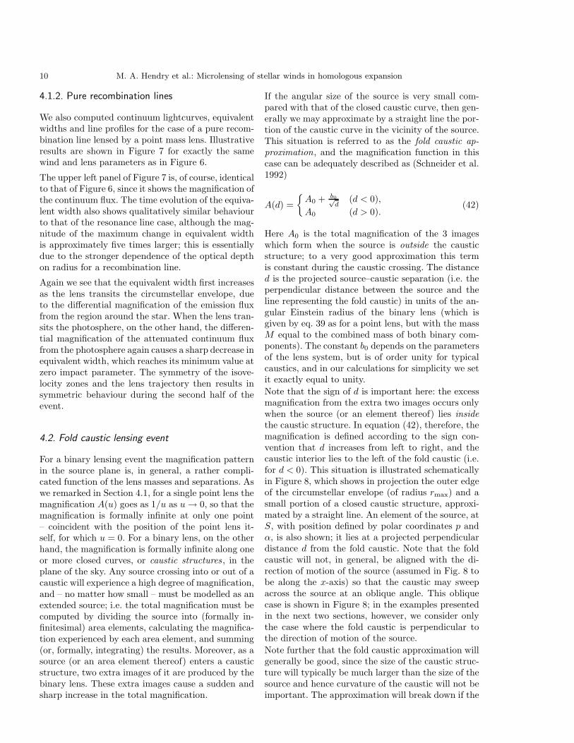
If the angular size of the source is very small com-pared with that of the closed caustic curve, then gen-erally we may approximate by a straight line the por-tion of the caustic curve in the vicinity of the source.This situation is referred to as the fold caustic ap-

proximation, and the magnification function in thiscase can be adequately described as (Schneider et al.1992)

A(d) =

A0 + b0√d

(d < 0),

A0 (d > 0).(42)

Here A0 is the total magnification of the 3 imageswhich form when the source is outside the causticstructure; to a very good approximation this termis constant during the caustic crossing. The distanced is the projected source–caustic separation (i.e. theperpendicular distance between the source and theline representing the fold caustic) in units of the an-gular Einstein radius of the binary lens (which isgiven by eq. 39 as for a point lens, but with the massM equal to the combined mass of both binary com-ponents). The constant b0 depends on the parametersof the lens system, but is of order unity for typicalcaustics, and in our calculations for simplicity we setit exactly equal to unity.

Note that the sign of d is important here: the excessmagnification from the extra two images occurs onlywhen the source (or an element thereof) lies inside

the caustic structure. In equation (42), therefore, themagnification is defined according to the sign con-vention that d increases from left to right, and thecaustic interior lies to the left of the fold caustic (i.e.for d < 0). This situation is illustrated schematicallyin Figure 8, which shows in projection the outer edgeof the circumstellar envelope (of radius rmax) and asmall portion of a closed caustic structure, approxi-mated by a straight line. An element of the source, atS, with position defined by polar coordinates p andα, is also shown; it lies at a projected perpendiculardistance d from the fold caustic. Note that the foldcaustic will not, in general, be aligned with the di-rection of motion of the source (assumed in Fig. 8 tobe along the x-axis) so that the caustic may sweepacross the source at an oblique angle. This obliquecase is shown in Figure 8; in the examples presentedin the next two sections, however, we consider onlythe case where the fold caustic is perpendicular tothe direction of motion of the source.

Note further that the fold caustic approximation willgenerally be good, since the size of the caustic struc-ture will typically be much larger than the size of thesource and hence curvature of the caustic will not beimportant. The approximation will break down if the


O

p

S

dL

y

x

Fig. 8. A schematic view of the source plane for a foldcaustic crossing event, showing in projection (i.e. with theobserver in the z direction) the outer edge of the circum-stellar envelope (of radius rmax). The bold line representsa small portion of a closed caustic structure, approxi-mated by a straight line. An element of the source, atS, with position defined by polar coordinates p and α,is shown; it lies at a projected perpendicular distance d

from the fold caustic. Note that the fold caustic will not,in general, be aligned with the direction of motion of thesource (assumed here to be along the x-axis) so that thecaustic may sweep across the source at an oblique angle.

caustic crossing occurs close to a ‘cusp’ in the caus-tic structure, but we do not consider that case here.We will extend our treatment to more general causticmodels (and to other expansion laws) in future work.

4.2.1. Pure resonance lines

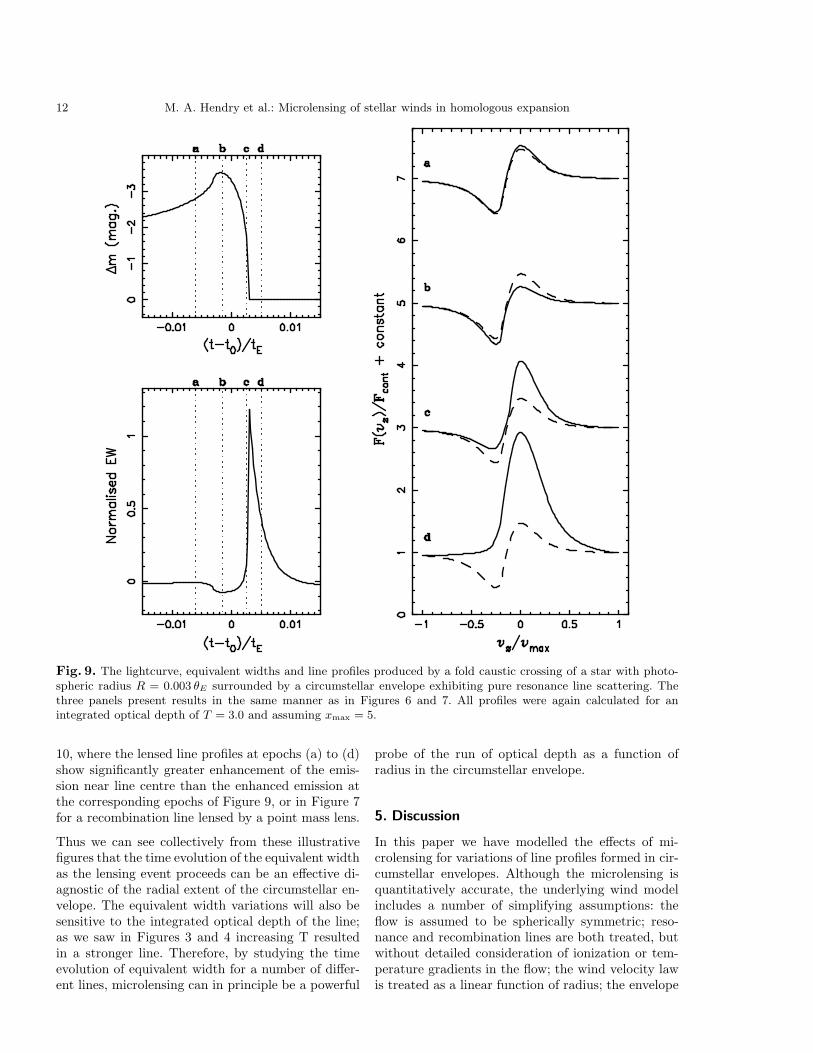
We next computed continuum lightcurves, line equiv-alent widths and line profiles for the case of a pureresonance line lensed by a fold caustic as the sourceexits the caustic structure. Illustrative results areshown in Figure 9 for a star with pseudo-photosphericradius R = 0.003 θE and assuming xmax = 5. Themodel line profile shown has T = 3.

The upper left hand panel of Figure 9 shows thechange in apparent magnitude, computed from theratio of lensed to unlensed continuum flux, as a func-tion of time (again measured in units of tE). Notethat we consider here only the effect of the excessmagnification due to the extra images produced bythe caustic structure; in other words we are assumingthat the term A0 in equation (42) is a constant duringthe caustic crossing, and can therefore be subtracted

from the total magnification, leaving only the differ-ential effect of the two extra images. Hence the mag-nitude change due to the extra images alone drops tozero after the photosphere has fully exited the foldcaustic.

The lower left hand panel of Figure 9 shows the timeevolution of the line equivalent width, calculated asbefore. We see that the equivalent width first risesgently as the fold caustic begins to cross the circum-stellar envelope and differentially magnifies the lineemission from the wind relative to the continuum.The increase in equivalent width is at first modest,however, because the absorption components of theline profile also receive some differential magnifica-tion at this stage. Indeed once the fold caustic be-gins to cross the star, the dominant effect of thedifferential magnification is to enhance the attenu-ated continuum flux from the pseudo-photosphere– thus resulting in a sharp dip in the equivalentwidth which reaches its minimum value at epoch (b).Thereafter the equivalent width begins to rise dra-matically. This is because an increasing fraction ofthe pseudo-photosphere now lies outside the causticstructure, so that the relative effect of the lens on thecircumstellar material which still lies inside is signif-icantly enhanced. This effect reaches its peak shortlyafter epoch (c), by which time the photosphere liesentirely outside the caustic but a portion of the cir-cumstellar envelope still lies inside, and thus contin-ues to be differentially magnified due to the existenceof the two extra images. As the fold caustic thensweeps across the rest of the envelope, the equiva-lent width drops sharply again, although at epoch (d)the equivalent width is still somewhat larger than atepoch (c) – as is evident in the profiles shown in theright hand panel.

4.2.2. Pure recombination lines

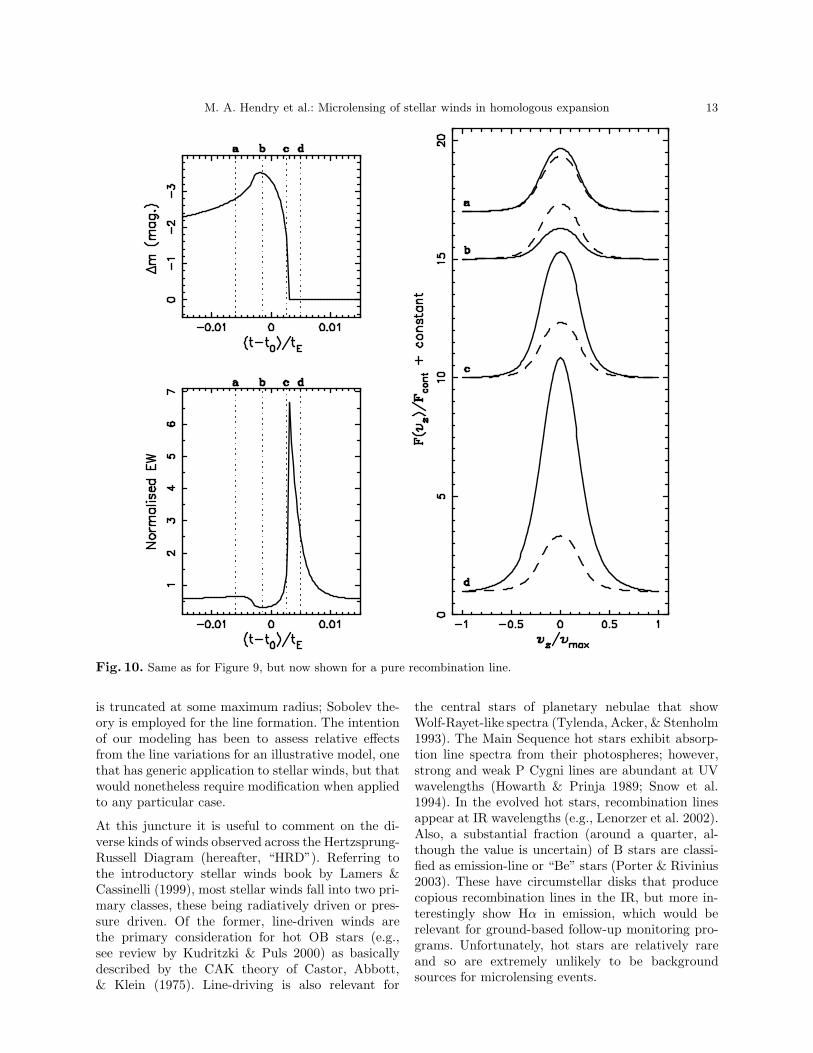
Finally we computed continuum lightcurves, lineequivalent widths and line profiles for the case of apure recombination line lensed by a fold caustic asthe source exits the caustic structure. Illustrative re-sults are shown in Figure 10 for eaxctly the same lensand source parameters as in Figure 9.

The upper left panel of Figure 10 is again identical tothat of Figure 9. From the lower left panel we see thatthe time evolution of the line equivalent width showsqualitatively similar behaviour to that of Figure 9,although again the magnitude of the change in equiv-alent width is significantly larger for a recombinationline than for a resonance line – as we also found fora point lens event. The stronger signature of lensingis also clearly seen in the right hand panel of Figure


Fig. 9. The lightcurve, equivalent widths and line profiles produced by a fold caustic crossing of a star with photo-spheric radius R = 0.003 θE surrounded by a circumstellar envelope exhibiting pure resonance line scattering. Thethree panels present results in the same manner as in Figures 6 and 7. All profiles were again calculated for anintegrated optical depth of T = 3.0 and assuming xmax = 5.

10, where the lensed line profiles at epochs (a) to (d)show significantly greater enhancement of the emis-sion near line centre than the enhanced emission atthe corresponding epochs of Figure 9, or in Figure 7for a recombination line lensed by a point mass lens.

Thus we can see collectively from these illustrativefigures that the time evolution of the equivalent widthas the lensing event proceeds can be an effective di-agnostic of the radial extent of the circumstellar en-velope. The equivalent width variations will also besensitive to the integrated optical depth of the line;as we saw in Figures 3 and 4 increasing T resultedin a stronger line. Therefore, by studying the timeevolution of equivalent width for a number of differ-ent lines, microlensing can in principle be a powerful

probe of the run of optical depth as a function ofradius in the circumstellar envelope.

5. Discussion

In this paper we have modelled the effects of mi-crolensing for variations of line profiles formed in cir-cumstellar envelopes. Although the microlensing isquantitatively accurate, the underlying wind modelincludes a number of simplifying assumptions: theflow is assumed to be spherically symmetric; reso-nance and recombination lines are both treated, butwithout detailed consideration of ionization or tem-perature gradients in the flow; the wind velocity lawis treated as a linear function of radius; the envelope


Fig. 10. Same as for Figure 9, but now shown for a pure recombination line.

is truncated at some maximum radius; Sobolev the-ory is employed for the line formation. The intentionof our modeling has been to assess relative effectsfrom the line variations for an illustrative model, onethat has generic application to stellar winds, but thatwould nonetheless require modification when appliedto any particular case.

At this juncture it is useful to comment on the di-verse kinds of winds observed across the Hertzsprung-Russell Diagram (hereafter, “HRD”). Referring tothe introductory stellar winds book by Lamers &Cassinelli (1999), most stellar winds fall into two pri-mary classes, these being radiatively driven or pres-sure driven. Of the former, line-driven winds arethe primary consideration for hot OB stars (e.g.,see review by Kudritzki & Puls 2000) as basicallydescribed by the CAK theory of Castor, Abbott,& Klein (1975). Line-driving is also relevant for

the central stars of planetary nebulae that showWolf-Rayet-like spectra (Tylenda, Acker, & Stenholm1993). The Main Sequence hot stars exhibit absorp-tion line spectra from their photospheres; however,strong and weak P Cygni lines are abundant at UVwavelengths (Howarth & Prinja 1989; Snow et al.1994). In the evolved hot stars, recombination linesappear at IR wavelengths (e.g., Lenorzer et al. 2002).Also, a substantial fraction (around a quarter, al-though the value is uncertain) of B stars are classi-fied as emission-line or “Be” stars (Porter & Rivinius2003). These have circumstellar disks that producecopious recombination lines in the IR, but more in-terestingly show Hα in emission, which would berelevant for ground-based follow-up monitoring pro-grams. Unfortunately, hot stars are relatively rareand so are extremely unlikely to be backgroundsources for microlensing events.


Working toward cooler temperatures in the HRD,the winds from Main Sequence stars A–M are notwell-studied, in part because their mass loss is somuch weaker than early-type stars. The yellow hy-pergiants have more substantial winds, but thesestars are extremely rare (de Jager 1998). A sub-class of the A stars are strongly magnetic – the Apand Am stars. These represent ∼ 10% of the A-star class (MacGregor 2005), and are stars with sur-face magnetic fields in the multi-kilo-Gauss range,often modelled as oblique magnetic rotators in whichthe magnetic field is predominantly dipolar (Stibbs1950). The wind diagnostics, particularly the por-tion trapped by the global dipolar magnetic fieldloops, are likely to be found in the X-ray band,as the trapped wind streams from opposite hemi-spheres are forced by the magnetic field into super-sonic collisions to generate shock-heated gas (e.g.,Babel & Montmerle 1997; Townsend & Owocki 2005).Again, these types of stars are not often expected infinite-source microlensing events. The solar-type starobserved in the extended source event reported inAbe et al. (2003) presumably has a solar-like stellarwind, with a feeble mass-loss rate of order 10−14 M⊙yr−1. Consequently, wind spectral features accessi-ble to ground-based follow-up would be essentiallynon-existent for such a source; instead, coronal diag-nostics would be found in the UV and X-ray bands.Although one might expect to see effects in Ca ii Hand K that are sensitive to chromospheric emission,our model line profiles are not appropriate for thequasi-static chromosphere.

The most likely class of stars to be found as sourcesin microlensing transit events, either by a single ora binary lens, are the red giant stars, a consequenceof their being reasonably common and fairly large insize. Red giant winds have modest mass-loss rates oforder 10−10 or 10−8M⊙ yr−1; however, even theseestimates are not certain because the origin of theirwinds is not well-understood. The absence of X-rayemission for K and M giants (Linsky & Haisch 1979)indicates that their winds are not Parker-like, al-though they do show chromospheric features. Thestrong Mg ii h and k lines and Fe ii lines can beused to probe cool star winds; however, these linesare found in the UV which is not amenable to ground-based follow-up. It may be that a combination ofmolecular opacity and some dust formation drives thewinds of red giants (Jorgensen & Johnson 1992), andperhaps certain molecular lines could be used as winddiagnostics.

Red supergiants (RSG) and asymptotic giant branch(AGB) stars have more interesting wind features thatcould be studied in microlensing transits. These are

stars with high mass-loss rates of order 10−5M⊙ yr−1.They are radiatively driven, but unlike the early-typestars that are line driven, these stars are continuumdriven because of substantial dust formation in theirdense and cool winds. Simmons et al. (2002) haveexplored the possibility that scattering polarizationcould be used to probe their winds, but of coursethis is a continuous opacity. Similar to the red giants,UV lines can be used to probe the wind flow. Some ofRSG and AGB stars also show maser emission lines atradio frequencies (Elitzur 1992; Habing 1996; Lewis1998). These are thought to form primarily in shells.Consequently, the model lines presented in this paperare less likely to be relevant, although the consid-erations of Ignace & Hendry (1999) might be moreappropriate, if suitably modified for the emissivityfunction of the maser. Once again, stars of the RSGand AGB classes are fairly rare.

There are two other classes of sources for which ourline profile models are more relevant. One is the ac-tive galactic nuclei (AGN) that produce strong windflows (Arav et al. 1995; Proga, Stone, & Kallman2000). The (rest frame) UV spectra of quasars showsome quite strong P Cygni profiles, such as in Civ, suggesting wind speeds in excess of 10,000 kms−1. The flows are likely line-driven similar to early-type stars. Already, some authors have modelledthe characteristic emission line profile effects thatwould be observed for different source models duringmicrolensing events (Popovic, Mediavilla, & Munoz2001; Abajas et al. 2002), ranging from Kepleriandisks to relativistic disks to simple shells and jets.The microlensing under consideration was by a singledeflector; however, our spherically symmetric windmodels are not directly applicable to these cases thatmostly involve non-spherical geometries. Some haveclaimed the detection of microlensing effects relevantto probing the AGN accretion disk (e.g., Chae et al.2001), although none have reported effects pertinentto a wind component. We will not discuss this classfurther, and have mentioned it only because the gen-eral consideration of emission profile variations dur-ing microlensing events involving wind flows has beenconsidered in the context of AGN.

The second class of objects are supernovae (and thelikely related gamma-ray bursters). The explosionsof stars spew gaseous ejecta into space. There is aphase in which the ejecta follows homologous expan-sion, not because the flow is accelerating, but becausethe ejecta is moving outward with a distribution ofspeeds. Still, the flow can be modeled as a wind,and the spectra at different phases shows numerouswind-features, ranging from strong P Cygni lines, torecombination lines, to forbidden lines (Filippenko


1997). Because supernovae (SNe) are so intrinsicallyluminous at early times, they can be seen to largedistances, and so the probability of lensing increasesowing to the considerable cosmological path lengthsinvolved.

Recently Dalal et al. (2003) have discussed the im-pact of weak lensing due to large scale structureon the use of SNe as standard candles. Other au-thors have considered microlensing as a tool forstudying the ejecta of SNe and even gamma-raybursts (GRBs). For example, Schneider & Wagoner(1987) considered polarimetric variations of pseudo-photospheres produced in SNe during a microlens-ing event. Bagherpour, Branch, & Kantowski (2005)modelled the impact of microlensing on P Cygni lineprofiles in the spectra of Type Ia SNe. Gaudi, Granot,& Loeb (2001) have invoked microlensing to explain abrightening event in the lightcurve of GRB-000301C.However, thus far a more comprehensice study thatsystematically explores the effects of microlensing onemission line features formed in SN and GRB ejectaremains to be made; our illustrative results presentedhere are a further step in that direction.

With respect to SNe, there are several points of cau-tion to be made when applying the results of this pa-per. First, our models assume a steady-state source.Of course, the luminosities, ejecta optical depth, andphotospheric radii evolve with time in real SNe. Ourresults are applicable to SNe if the lensing event isrelatively fast compared to photometric and struc-tural changes of the ejecta. Under what conditionswill this be true? Suppose we take the duration ofthe lensing event to be one week. If the fastest ejectashell moves at 104 km s−1, then the extent of theejecta shell would be at least rmax ≈ 40 AU at earlyphases of the explosion in which homologous expan-sion is applicable. Moreover, the evolution must besuch that the lens moves across the ejecta shell (inprojection) before the dimensions of the photospherechange significantly. This means the proper motionof the lens should greatly exceed that of the photo-spheric expansion. Given the 104 km s−1 ejecta speedas a maximum, and assuming a transverse velocityof 102 km s−1 for the lensing mass, we require thatDSN ≫ DL. Consequently, if the lens were locatedat kpc distances (e.g., in the halo, the bulge, or theLarge Magellanic Cloud), then the SN should be lo-cated at Mpc distances (e.g. at the distance of theVirgo cluster).

As a consistency check, we compare the angular sizeof the SN ejecta θSN to θE, as given by

θSN

θE=

rmax/DSN√

(RL/DL) (1 − DL/DSN). (43)

If we assume the lensing object to be typical ofMACHOs of about 0.5M⊙, then the Schwarzschildradius of the lens RL will be of order 1 km. If wefurther assume rmax ≈ 40 AU, and DSN ≫ DL, then

θSN

θE≈ 100 kpc

DSN, (44)

where DL = 10 kpc was assumed. Thus, SNe atdistances of several to dozens of Mpc would haveθSN/θE ≈ 0.01 − 0.1 at early phases in the SN whenhomologous expansion remains valid. These happento be values typical of our model simulations.A further assumption of our models has been thecommon “core-halo” treatment, in which we can ap-proximate the photosphere as a “hard” sphericalboundary, and the wind features are all formed exte-rior to this boundary. Recent radiative transfer sim-ulation of Type II SNe by Dessart & Hillier (2005)show this not to be true. Instead, the radiative trans-fer in SNe ejecta is more akin to that of Wolf-Rayetstars, for which the continuum forms in the wind flow.The purpose of our models has not been to repre-sent rigorously any particular type of stellar wind orclass of stars, but to illustrate the generic effects thatcould be observed with intensive follow-up programsfor source transit microlensing events. In so doing,models for two common types of lines have been con-sidered – resonance P Cygni lines and recombina-tion emission lines, for both point lensing and caus-tic crossing events from binary lensing. Whether thesource is a hot star or a cool star, whether the linesare in the X-ray band or the radio band, the generalproperties of the line variations in terms of lead/lagtimes relative to the photosphere, of equivalent widthvariations, and changes in line profile shape are qual-itatively all to be expected. We imposed the homolo-gous expansion as a representative flow velocity law.Observationally, the velocity law is something thatwould preferably be determined from the line vari-ations as the microlensing event evolved. With thephotospheric crossing time determined from the pho-tometric variations, the variations of the line equiv-alent width and profile changes with time could beconverted to radius, calibrated by the photosphericradius, to deduce flow velocity and opacity variations.

Acknowledgements. R. Ignace gratefully acknowledgessupport for this work by a NSF grant, AST-0354262. Theauthors gratefully acknowledge the helpful comments ofthe anonymous referee.

References

Abajas C., Mediavilla E., Munoz J. A., Popovic L. C.,Oscoz A. 2002, ApJ 576,


be F., Bennett D. P., Lgerkvist C. I, et al. A&A, 411, 493Afonso C., Alard C., Albert J.N. et al. 2000, ApJ, 532,

340Albrow M., Beaulieu J. P., Birch P. et al. 1998, ApJ, 509,

687Albrow M., Beaulieu J. P., Caldwell J. A. R. et al. 1999,

ApJ, 522, 1022Albrow M., Beaulieu J. P., Caldwell J. A. R. et al. 2000,

ApJ, 534, 894Albrow M., An J., Beaulieu J. P. et al. 2001a, ApJ, 549,

759Albrow M., An J., Beaulieu J. P. et al. 2001b, ApJ, 550,

173Alcock C., Allen W. H., Allsman R. A. et al. 1997, ApJ

491, 436Arav N., Korista K. T., Barlow T. A., Begelman M. C.

1995, Nat. 376, 576Babel, J., Montmerle, T. 1997, A&A 323, 121Bagherpour, H., Kantowski, R., Branch, D., Richardson,

D. 2004, astro-ph/0411622Bagherpour, H., Branch, D., Kantowski, R. 2005,

astro-ph/0503460Bryce H. M., Ignace, R., Hendry, M. A. 2003, A&A, 401,

339Castor, J. I., Abbott, D. C., Klein, R. I. 1975, ApJ 195,

157Chae, K.-H., Turnshek, D. A., Schulte-Ladbeck, R. E.,

Rao, S. M., Lupie, O. L. 2001, ApJ 561, 653Coleman, I. J., Simmons, J. F. L., Newsam, A. M.,

Bjorkman, J. E. 1997. In: Ferlet, R. et al. (eds.)Variable Stars and the Astrophysical Returns of theMicrolensing Surveys (Editions Frontieres) p. 147

Coleman, I. J. 1998, Ph.D. Thesis, University of GlasgowDalal, N., Holz, D. E., Chen, X., Frieman, J. A. 2003,

ApJ, 585, 11de Jager, C. 1998, A&ARv 8 145Dessart, L., Hillier, D. J. 2005, A&A 437, 667Elitzur, M. 1992, ARAA 30, 75Fields, D. L., Albrow, M. D., An, J. et al. 2003, ApJ, 596,

1305Filippenko, A. V. 1997, ARAA 35, 309Gaudi, B. S., Granot, J., Loeb, A. 2001, ApJ 561, 178Gould A. 2001, PASP 113, 903Habing, H. J. 1996, A&ARv, 7, 97Hauschildt, P. H., Allard F., Baron E. 1999, ApJ, 525,

871Heyrovsky, D., Sasselov, D., Loeb, A. 2000, ApJ, 543, 406Howarth, I. D., Prinja, R. K. 1989, ApJS 69, 527Ignace, R., Hendry, M. A. 1999, A&A, 341, 201Jorgensen U. G., Johnson H. R. 1992, A&A 265, 168Kudritzki, R.-P., Puls, J. 2000, ARAA 38, 613Kurucz, R. L. 1994, Atlas CDROMs (Email: ku-

[email protected])Lamers, H., Cassinelli, J. 1999, Introduction to Stellar

Winds (Cambridge University Pres)Lenorzer, A., Vandenbussche, Morris, P. 2002, A&A 384,

473Lewis, B. M. 1998, ApJ 508, 831Linksy, J. L, Haisch, B. M. 1979, ApJ 229, L27

MacGregor, K. B. 2005, in The Nature and Evolution ofDisks Around Hot Stars, Ignace and Gayley (eds.),ASP Conf. Ser. 337, 28

Mihalas D. 1978, Stellar Atmospheres, (Freeman: NewYork)

Paczynski B. 1986, ApJ, 304, 1Popovic, L. C., Mediavilla, E. G., Munoz, J. A. 2001,

A&A, 378, 295Porter, J. M., Rivinius, Th. 2003, PASP 115, 1153Proga, D., Stone, J. M., Kallman, T. R. 2000, ApJ 543,

686Schneider, P., Wagoner, R. V. 1987, ApJ 314, 154Schneider, P., Ehlers, J., Falco, E. E. 1992, Gravitational

Lenses (Springer-Verlag)Simmons, J. F. L., Bjorkman, J. E., Ignace, R., Coleman,

I. J. 2002, MNRAS 336, 501Snow, T. P., Lamers, J. G. L. M., Lindholm, D. M., Odell,

A. P. 1994, ApJS 95, 163Stibbs, D. W. N. 1950, MNRAS 110, 395Townsend, R. H. D., Owocki, S. P. 2005, MNRAS 357,

251Tylenda, R., Acker, A., Stenholm, B. 1993, A&AS 102,

595

http://arXiv.org/abs/astro-ph/0411622

http://arXiv.org/abs/astro-ph/0503460

microlensing of circumstellar envelopes. iii. line profiles from stellar winds in homologous...

Documents