microfinance, vulnerability and risk in low income households

This article was downloaded by: [Uppsala universitetsbibliotek]On: 02 November 2014, At: 02:32Publisher: RoutledgeInforma Ltd Registered in England and Wales Registered Number: 1072954 Registeredoffice: Mortimer House, 37-41 Mortimer Street, London W1T 3JH, UK

International Review of AppliedEconomicsPublication details, including instructions for authors andsubscription information:http://www.tandfonline.com/loi/cira20

Microfinance, vulnerability and risk inlow income householdsRanjula Bali Swaina & Maria Florob

a Department of Economics, Uppsala University, Uppsala, Swedenb Department of Economics, American University, NW Washington,DC, USAPublished online: 06 Jun 2014.

To cite this article: Ranjula Bali Swain & Maria Floro (2014) Microfinance, vulnerability andrisk in low income households, International Review of Applied Economics, 28:5, 539-561, DOI:10.1080/02692171.2014.918937

To link to this article: http://dx.doi.org/10.1080/02692171.2014.918937

PLEASE SCROLL DOWN FOR ARTICLE

Taylor & Francis makes every effort to ensure the accuracy of all the information (the“Content”) contained in the publications on our platform. However, Taylor & Francis,our agents, and our licensors make no representations or warranties whatsoever as tothe accuracy, completeness, or suitability for any purpose of the Content. Any opinionsand views expressed in this publication are the opinions and views of the authors,and are not the views of or endorsed by Taylor & Francis. The accuracy of the Contentshould not be relied upon and should be independently verified with primary sourcesof information. Taylor and Francis shall not be liable for any losses, actions, claims,proceedings, demands, costs, expenses, damages, and other liabilities whatsoever orhowsoever caused arising directly or indirectly in connection with, in relation to or arisingout of the use of the Content.

This article may be used for research, teaching, and private study purposes. Anysubstantial or systematic reproduction, redistribution, reselling, loan, sub-licensing,systematic supply, or distribution in any form to anyone is expressly forbidden. Terms &Conditions of access and use can be found at http://www.tandfonline.com/page/terms-and-conditions

http://www.tandfonline.com/loi/cira20

http://www.tandfonline.com/action/showCitFormats?doi=10.1080/02692171.2014.918937

http://dx.doi.org/10.1080/02692171.2014.918937

http://www.tandfonline.com/page/terms-and-conditions

http://www.tandfonline.com/page/terms-and-conditions

Microfinance, vulnerability and risk in low income households

Ranjula Bali Swaina* and Maria Florob

aDepartment of Economics, Uppsala University, Uppsala, Sweden; bDepartment ofEconomics, American University, NW Washington, DC, USA

(Received 4 April 2012; final version received 14 April 2014)

We investigate if participation in the Indian Self Help Group (SHG) programresults in reducing poverty and vulnerability. The theoretical framework exam-ines the mechanisms through which the pecuniary and non-pecuniary effects ofthe SHG impacts the households’ ability to manage risk. We use a vulnerabilitymeasure that quantifies the welfare loss associated with poverty and differenttypes of risks, on an Indian panel survey data. Our results show that SHG mem-bers are less vulnerable compared with a group of non-SHG (control) members.About 80% of the vulnerability faced by the households is poverty related.

Keywords: microfinance; vulnerability; poverty; risk coping

JEL Classifications: D14, G21, I32

1. Introduction

In recent years there has been growing concern on the extent of vulnerability amonglow-income households. Much of this concern is related to the effect of market liber-alization policies that accompanied globalization trends. Since the early 1990s, Indiareversed the state-led economic policies that had characterized its economy in previ-ous decades (Little and Joshi 1994). Precipitated by the 1991 balance of paymentscrisis and high levels of debt, the Indian government opened up the economy, gavethe market a greater role in price setting by liberalizing interest rates, and increasedthe private sector’s role in development and market competition, following the loanconditionalities of the World Bank and IMF. The intent of these reforms was tospeed up growth and thereby reduce poverty (Sen and Vaidya 1997; World Bank2000).

Thus far, these expectations have not been fulfilled, given the persistence of pov-erty amidst the economic growth experienced by India in recent years. Moreover,there is increasing concern that the impact of these policies has adverse distribu-tional consequences. The Gini index has risen from 30 to almost 38 from 1991 to1997. In 2005, the Gini coefficient for India was calculated at between 0.37 and0.42, according to varying estimates. The distributive allocation of risk associatedwith market liberalization is likely to be more problematic for poor households. Theinsecurity of incomes in the current macroeconomic environment has far-reachingeffects in terms of inducing vulnerability especially among rural, asset poor house-holds. Income variability that arises from fluctuations in harvests, farm input and

*Corresponding author. Email: [email protected]

© 2014 Taylor & Francis

International Review of Applied Economics, 2014Vol. 28, No. 5, 539–561, http://dx.doi.org/10.1080/02692171.2014.918937

Dow

nloa

ded

by [

Upp

sala

uni

vers

itets

bibl

iote

k] a

t 02:

32 0

2 N

ovem

ber

2014

mailto:[email protected]

http://dx.doi.org/10.1080/02692171.2014.918937

output prices and informal, non-farm employment affects the households’ ability tomanage risk. Thus, even though average household incomes do not fall into povertylevels, their degree of vulnerability can be high, creating problems of borrowing,repaying debt and managing risk.

In this regard, there has been an increased interest on the role of community-based organizations such as microfinance programs to address these concerns andneeds of poor households that markets and governments fail to adequately meet.More specifically, a growing number of studies have examined the extent to whichself-help microfinance groups characterized by decentralized manner of interactionas well as participatory decision-making processes enable them to be receptive tothe needs of women in poor households and thereby help alleviate poverty (BaliSwain and Floro 2012; Ackerly 1997; Amin, Rai, and Topa 1999; De Aghion andMorduch 2006; Goetz 1997; Morduch 1999; Pitt and Khandker 1998; Puhazhendiand Badatya 2002; Sebstad and Cohen 2001). The issue of women’s empowermenthas also been addressed in studies on women-focused microfinance programs(Mayoux 2002; Rankin 2002). There remains, however, the question of whether, byproviding financial and other related services to rural households, these groups areeffective in reducing their vulnerability thereby enabling households to make pro-ductive investment and not withdraw critical resources in times of income or expen-diture shocks. Microfinance organizations can affect household outcomes through avariety of channels. These include the direct income effect, indirect income effectthrough non-financial benefits such as added training and education and, nonpecuni-ary effects such as strengthened social networks and better self-esteem (de Aghionand Morduch 2006). Recent studies have expressed concerns regarding the adequacyof income-poverty measures alone in understanding vulnerability (Calvo and Dercon2005; Carter and Ikegami 2007; Dercon and Krishnan 2000; Dercon 2005; Glewweand Hall 1998; Ligon and Schechter 2002). The cumulative impact of microfinanceorganizations on household vulnerability may therefore not be captured by standardincome poverty measures alone.

Our objectives in this paper are twofold. One is to examine an important dimen-sion of household welfare that conventional measures of poverty do not address,namely the ability of households to cope with risk, particularly the risk of experienc-ing food shortage. In particular, we want to understand the realities pertaining to theeconomic situation of rural low-income households by exploring the determinants ofvulnerability to hunger. Vulnerability in our study is defined as a high degree ofexposure to risks, shocks and proneness to food insecurity that can undermine thehousehold’s survival and the development of its members’ capabilities. Our secondaim is to explore directly the link between self-help microfinance groups (SHG) andvulnerability. Using a panel data drawn from a sample survey among SHG and non-SHG households in rural India in early 2000, we examine whether or not a house-hold member’s participation in SHG reduces household vulnerability. We firstdevelop a theoretical model that explores the risk-coping mechanism through whichSHG participation can result in a decline in household vulnerability. We then takeinto account the varied sources of vulnerability by constructing a vulnerability mea-sure that draws from the work of Ligon and Schechter (2003) and that helps esti-mate the welfare loss associated with poverty as well as from aggregate andidiosyncratic risks that expose households to consumption shocks. The householdsample survey data provides detailed information on consumption, variability inincomes, credit, and relevant household and individual characteristics for two time

540 R. Bali Swain and M. Floro

Dow

nloa

ded

by [

Upp

sala

uni

vers

itets

bibl

iote

k] a

t 02:

32 0

2 N

ovem

ber

2014

periods, namely 2000 and 2003. Its sampling design enables us to compare theeconomic situation between SHG beneficiaries (treatment group) and non-SHGbeneficiaries (control group).

India’s National Bank for Agriculture and Rural Development (NABARD 2006)started the self-help group (SHG)–bank linkage program in 1992 and since then, hasbecome the largest microfinance program in the developing world. Mainly targetingwomen, by 31 March 2010, about seven million SHGs had saving accounts andmore than 4.9 million were credit linked with about 97 million poor households cov-ered under this microfinance program.1 Even though the rapid pace of SHG outreachhas slowed down in recent years, SHGs were still growing about twice as fast ascompared with other Indian microfinance institutions in 2008–2009 (Srinivasan2011). The SHGs continue to hold a dominating position in the Indian microfinancesector, with the government claiming the SHG program as a crucial poverty allevia-tion strategy.

In recent years, microfinance programs have been critically investigated and theirassessment has given mixed results (Armendariz and Morduch 2010; Dichter andHarper 2007; Karlan 2007). The adverse impact of several microfinance institutions(MFIs) in India has raised questions regarding the overall contribution of such pro-grams towards poverty reduction. MFIs, particularly those that are commercialbank-initiated, have been criticised for their negative impact on the economic situa-tion of small farmers and near-landless households in terms of rising indebtednessand interest rates (Ghate et al. 2007; Srinivasan 2010).

Section 2 discusses the notion of vulnerability and the varied measures used in anumber of studies. By examining the pecuniary and the non-pecuniary effects ofSHGs, we then develop a theoretical model that explores how participation in theSHG program may influence a household’s ability to manage risk, thereby resultingin declining vulnerability. Section 3 briefly discusses the Ligon and Schechter vul-nerability measure that we utilize and provides an overview of the sample data usedin the analysis along with the main empirical results. We show that vulnerability issignificantly lower among households who belong to SHG (treatment group) com-pared with those who are not (control group), thus supporting the view that microfi-nance programs such as the SHGs have the potential to reduce vulnerability whensocial objectives remain predominant and program products address the needs of thebeneficiaries. The paper concludes with policy implications and suggestions towardsa better understanding of vulnerability.

2. Vulnerability and risk

2.1. Understanding risk and vulnerability

While vulnerability is defined in a number of ways, we define it here in terms of thehousehold and its members’ ability to deal with risks, shocks and proneness to foodsecurity and hence their attitude towards undertaking risks.2 When households facesuch multitudes of risks, they are prone to severe hardship so that the subjectiveprobability attached by household members towards adverse outcomes is likely tobe high.

Vulnerability is prevalent in rural low income households as several studieshave shown because the magnitude of risk that they face is striking, particularly forthose who live in the rain-fed areas and their subjective judgment regarding the

International Review of Applied Economics 541

Dow

nloa

ded

by [

Upp

sala

uni

vers

itets

bibl

iote

k] a

t 02:

32 0

2 N

ovem

ber

2014

likelihood of shocks is high. The threat of loss of or decline in farm earnings isbrought about by environmental conditions that affect their output, such as weather,leading to drought or floods, pests, and by market fluctuations that lead to changesin input and product prices. Yield risks are especially significant when agriculturalprice and other supports are inadequate or non-existent. There are other types of riskas well, induced by the possibility of income decline in non-farm activities. In addi-tion, unexpected shocks due to illness, death, etc. are anticipated given the health-related environment and poor medical services situation they face. These shocks canlead to substantial loss of income, wealth and/or consumption. These risks translateinto such commonplace concerns as being able to eat three meals a day, being ableto afford to pay school fees for children, to seek medical assistance when ill, to buyinputs and even to repay loans. Vulnerability therefore relates to the claims or rightsover resources in dealing with risk, shocks, and economic stresses.

It is now widely acknowledged that a major aspect of people’s livelihoodsinvolves mechanisms to cope with risk and shocks. Hence, households will makecertain decisions in anticipation of or to mitigate the threat to its well-being offailure or occurrence of shock. Rural, low-income households in particular havedeveloped a number of mechanisms to buffer themselves from, or at least mini-mize the effects of, shocks (Dercon 2005; Zimmerman and Carter 2003). Theseinclude reciprocity agreements; the use of assets as buffer stocks; multiple crop-ping, and other livelihood diversification strategies. First, households have mecha-nisms to cope ex post with shocks, to smooth consumption and nutrition whenshocks happen, even if formal credit markets and insurance are not available.They may use savings, often in the form of live animals, built up as part of aprecautionary strategy against risk, or engage in informal mutual support net-works, for example, clan or neighbourhood based or even more formal groupssuch as funeral societies.

As Zimmerman and Carter (2003) have shown in their study on asset smoothing,low-income households will even do some trade-off between a higher incomeinvolving greater probability of income failure (and higher debt) and a lower incomeinvolving smaller probability of income failure. In other words, there is tendency tobe risk averse, which means that the households/individuals are prepared to acceptlower income for greater security, when the risk of having a bad outcome can seri-ously undermine household survival.

The presence of self-help microfinance groups such as those linked with theNational Bank for Agriculture and Rural Development NABARD in villages canhelp to some extent the member-households deal with or manage some risks, espe-cially in the absence of social protection or insurance schemes. For instance, mem-bers of a SHG may share each other’s risk through the institutionalizedarrangements, by providing loans to those members whose income is temporarilyrelatively low. Some studies on the effects of negative shocks or crises on poorhouseholds have demonstrated that microfinance schemes can play a role in con-sumption smoothing and in managing loss from shocks (Puhazhendi and Badatya2002). The loan provision component of self-help groups is one part of the riskmanagement and income generation feature that enables households to cope withbasic needs and contingencies of life.

In addition to the pecuniary effect of loan provisioning, SHGs can promote orhelp strengthen those social networks providing mutual support by facilitating thepooling of savings, regular meetings, etc. The non-pecuniary effect of SHGs can


Dow

nloa

ded

by [

Upp

sala

uni

vers

itets

bibl

iote

k] a

t 02:

32 0

2 N

ovem

ber

2014

help reduce the vulnerability of the members and, by association, that of theirhouseholds in ways that may not be adequately captured by a change in householdearnings. A growing number of studies on micro-credit have highlighted, for exam-ple, the empowerment effect on women members (Bali Swain 2007; Bali Swain andWallentin 2009). This involves a significant change in attitude, changes in workingpractices and challenging prevailing norms that constrains the ability of women topursue income-generating activities or other interests. Such constraints may bedirectly due, for example, to cultural ascriptions that prohibit women from workingoutside the home. But even without explicit constraints of this kind, the sociallyassigned roles of women to household responsibilities suggest that their ability toparticipate in income earning opportunities outside the household or farm is likely tobe more circumscribed or conditional than is the case for men (Bali Swain 2007).

Regular meetings and exchanges of SHG members can modify the constraintsand options of members and their families by reinterpreting or challenging socialprescriptions on permissible courses of action that women can take. SHGs provide aregular forum for women to come together to discuss their concerns and interests.Since questioning of prevailing norms does not happen automatically, it is the regu-larity of collective sharing of information and organizational skills/coping strategiesthat can eventually bring about a change in attitude, including dealing with risks.The impact of SHG therefore goes beyond provisioning of loans to meet any liquid-ity constraints faced by the household. Thus non-financial services such as trainingand participation in group meetings may impact the household’s ability to undertakerisk in productive investment. The overall effect of SHG on both the means and themanner in which households deal with risk can significantly affect the capabilitiesand entitlements of the household members in ways that are not captured by strictlyfinance-oriented program evaluation.

The effect on vulnerability is further captured by the non-pecuniary effect in theform of added resilience of SHG members, where resilience means the ability todeal with risk, particularly idiosyncratic risk, given the strengthened social supportscheme. Hence, NABARD-sponsored SHGs can reduce the vulnerability of themembers’ household not only through the income effect that increases consumptionlevels but also through their non-pecuniary effect that are not captured by focusingmerely on changes in incomes.

On the other hand, the characteristics of rural livelihoods in developing countriessuch as India often exhibit high correlations between risks faced by households inthe same village or area. Hence, when farm prices decline, or there is a drought orflood in the area, all households are adversely affected simultaneously. Group-basedsystems including SHGs are found to be ineffective in the face of ‘covariate’ shocks,including flooding or problem of declining crop prices or lack of demand for theirproduce.3 Thus, while SHG groups can be of help in cases when a household facesan idiosyncratic shock, the protection afforded by SHG in dealing with aggregateshocks is likely to be weak or partial. Moreover, the impact of SHGs on sociallyascribed rules that limit or constrain women in their choices and economic participa-tion may depend on the tenacity of such norms. The prevailing social institutionsthrough which women’s decisions and choices are mediated may be so overwhelm-ingly strong and resilient that they can still suppress opportunities for women. Thissocial embeddedness of individual or household actions need to be kept in mindwhen acknowledging the non-pecuniary impact of self-help microfinance groups. In


Dow

nloa

ded

by [

Upp

sala

uni

vers

itets

bibl

iote

k] a

t 02:

32 0

2 N

ovem

ber

2014

this case, one may observe that the resulting effect of SHG on vulnerability islimited.

2.2. Theoretical framework

We present a theoretical framework in this section that explains the decline in vul-nerability in the presence of uncertainty; and to show that SHG member householdsare likely to respond to risks or behave differently towards productive opportunitiesas compared with the non-SHGs (control households). Based on the discussion inthe previous section, we present a simple analytical framework for understandingthe effect of SHGs on household vulnerability. More specifically, we examine whyand how a household’s participation in a SHG may influence a household’s abilityto manage risk using a von Neumann–Morgenstern-based utility function to capturerisk preferences4 ‘expected utility” function as the basis for measuring vulnerability.Our hypothesis is that a household’s participation in SHG affects its household riskcoping ability not only by the increase in earnings in the current period due toenhanced access to credit but also by the member’s perceived future earnings andperceived risk. The latter is due to the non-pecuniary impact of SHG throughstrengthened social cohesion and increased empowerment of its members. Hence,participation in SHG, in addition to its pecuniary effect on expected future earnings,is likely to improve the household’s consumption smoothing ability so that per-ceived risk is lowered. To make our model comparable with the Ligon-Schechtermethodological approach to measuring vulnerability, we adopt some features of theirutility function, specifically the idea that household welfare (or expected utility) isan increasing, concave function of consumption expenditures, c.

We assume that each household i makes a decision on how much risk to under-take, given its propensity to manage it.5 We also assume that insurance markets arenon-existent and rural financial markets, (i.e. institutions that provide savings andcredit services) are segmented and likely to be less accessible to rural poor house-holds. We examine whether, for a given level of earning, a SHG-member household(S), is better able to cope with risk compared with a similar household that is not aSHG member (N). Consider the following household objective function in a two-period model that is a strictly increasing, weakly concave function:

Ui ¼ U ½ðci1;ci2Þ� (1)

where Ui refers to a household’s welfare or utility,6 ci is a vector of goods and ser-vices consumed by household i at period t. In the first period, ci1 is given by:

ci1 ¼ Y i1 � Ri

1 (2)

where Y i1 is income in the first period and Ri

1 are resources that are set aside andmade available to cope with any income shock or unanticipated expense. Theyinclude private savings as well as savings deposited in a self-help group, which pro-vides credit.

Household consumption in the second period is given by:

ci2 ¼ Y i2 þ Ri

1ð1þ rÞ (3)

where Y i2 is future income which is not known in period t = 1 For the SHG

members, Ri1 includes the savings deposited in the SHG, thus σ may be interpreted


Dow

nloa

ded

by [

Upp

sala

uni

vers

itets

bibl

iote

k] a

t 02:

32 0

2 N

ovem

ber

2014

as the nominal interest rate, where 0 < σ < 1. The non-SHG members on the otherhand, do not have the possibility to save with SHGs and tend to hold their savingsin cash (or some other form of savings) that do not earn interest. Thus, for the non-SHG members σ is a discount rate where –1 < σ < 0. For both SHGs and non SHGhouseholds, (1 + σ) > 0 nonetheless. The household’s beliefs about the level offuture income can be summarized in a subjective probability density function f (Y i

2)with mean ξ. On this basis we obtain the following expected objective function (inthe von Neumann–Morgenstern sense). Substituting equation (2) into equation (3),we can obtain:

ci2 ¼ Y i2 þ ðY i

1 � ci1Þð1þ rÞ (4)

So that the expected objective function is:

E½UiðcitÞ� ¼Z

U ½ci1;Y i2 þ ðY i

1 � ci1Þð1þ rÞ�f ðY i2ÞdY i

2 (5)

where integration is over the range of Y i2. Maximizing ci2 with respect to consump-

tion at t = 1, we obtain the first order condition,

D1 ¼ E½Ui1 � ð1þ rÞUi

2� ¼ 0 (6)

and the second-order condition,

D2 ¼ E½Ui11� � 2ð1þ rÞUi

12 � ð1þ rÞ2E½Ui22�\0 (7)

Differential access to credit as well as to savings facilities, can lead to differ-ences in incomes earned by SHG-member (i = S) and non-SHG member house-holds (i =N) in period 2. This is due to an increase in Ys due to an increase inproduction credit in t = 2. In particular,

YN2\YS

2 for household i (8)

If households’ expected future earnings are assumed to be the same, the effect ofan increase in income, say of Y i

1, can be found by implicit differentiation of equa-tion (6):

@ci1=Yi1 ¼ �ð1þ rÞE½Ui

12 � ð 1þ rÞUi22�= D2 [ 0 (9)

This implies that:

E½U i12 � ð1þ rÞUi

22�[ 0 (10)

Note, however, that the sign of equation (10) cannot be determined a priori in thecase where the expected or perceived future earnings of households are assumed todiffer, on the basis of their SHG participation. It is possible that even at lower levelsof income, SHG households use less of their resources compared with non-SHGhouseholds in order to deal with shocks. On the other hand, SHG households mayuse just the same amount or more of their resources if covariant shocks such asdrought or floods take place. In this case, the sign of equation (10) will beambiguous.

We next examine the effects of the differences in SHG and non-SHG house-holds’ probability density function of future income and household’s ability to copewith shocks. The risk coping function of household i can be written as:


Dow

nloa

ded

by [

Upp

sala

uni

vers

itets

bibl

iote

k] a

t 02:

32 0

2 N

ovem

ber

2014

Ri ¼ ai þ wiY i; i 2 S or N; and wi � 0 (11)

where Ri refers to the household’s resources that serve as the fall-back position ofthe household in the face of a shock, i.e. a decline in harvest, serious illness, etc.; ai

is the level of saving, credit and other resources available to the household i for cop-ing, which do not depend on participation in SHG, ψi is the propensity of a house-hold to deal with shock, and Yi is household income.7 A higher ψ reflects thehousehold’s ability to set aside a larger portion of household income in order to copewith shock. The more a household is able to cope with shocks, that is, the higherthe R, the less vulnerable is the household. In this sense, household welfare dependsnot just on its average income or expenditures, but on the risk it faces as well as itsaccess to resources in dealing with shocks.

Rather than assume that ψi is uniform across households, we explore the likeli-hood that participation in SHG not only leads to differences in household income Y i

due to the earnings effect. It also yields different subjective propensities,8 that is, forthe household i, the propensity of the household to cope with shock, ψi, is greater ifthe household is a SHG member. This is due to the non-pecuniary impact of SHGthrough strengthened social cohesion and increased empowerment of its members.The reasons for this difference, as discussed earlier, are varied. For illustrative pur-poses, and without loss of generality, we will focus on only two in this model. Theseare: (a) differences in perceived household income in the future resulting from pecu-niary (direct earnings) effect of SHG (call this П); and (b) differences in perceivedrisk resulting from their different levels of social support and cohesion (call this Ξ).The difference in perceived earnings is reflected in the agency function while thedifference in perceived risk is reflected in the ability to cope with unexpectedshocks, defined by the (subjective) probability distribution of future income f(Yi2)with mean ξ.

The SHG-member households’ strengthened mutual support system andimproved access to credit and savings facilities will cause SHG household’s proba-bility distribution of Y2 to differ from that of a non-SHG member. This is demon-strated by two kinds of shifts in the SHG’s probability distribution of Y2. One is anadditive shift, θ, which is equivalent to an increase in the mean with all othermoments constant. The other is a variance shift, γi, by which the distribution is moredispersed (or stretched) around zero. A higher dispersion in the probability distribu-tion of future income, as in the case for non-SHG, is equivalent to a stretching ofthe distribution around a constant mean – that is, a combination of additive and vari-ance parameter changes in the household’s probability distribution.

For the sake of simplicity, let us examine the effect on present consumptionsmoothing of a decrease in the perceived degree of risk concerning future incomefor a given household. Holding other factors constant, we then test whether adecrease in the SHG household’s uncertainty leads to an increase or decrease inpresent consumption, and hence, a decrease or increase in risk coping ability. Letthe expected value of future income for a household (we now drop the subscript i)be written as:

E½cY2 þ h� (12)

where γ is the variance shift parameter and θ is the additive one. Because Y2 ≥ 0, avariance shift around zero will increase the mean. This has to be counteracted by an


Dow

nloa

ded

by [

Upp

sala

uni

vers

itets

bibl

iote

k] a

t 02:

32 0

2 N

ovem

ber

2014

additive shift in the negative direction in order for the expected value to remain con-stant. Differentiating (12), the requirement is that:

dE½cY2 þ h�¼ E½Y2dcþ dh� ¼ 0; (13)

which implies:

dh=dc ¼ �E½Y2� ¼ �n (14)

We can now substitute equation (11) into the first-order condition (6), and thendifferentiate present consumption c1 with respect to γ, which yields:

ð@c1=@cÞ ¼ �1ð1=D2ÞE½ðU12 � ð1þ rÞU22ÞðY2 � nÞ�\0 (15)

Equation (15) shows that a decrease in perceived risk by a rural household, man-ifested as a decreased dispersion around future income, is likely to increase its riskcoping ability and hence increase its present consumption. (The proof of this resultis set out in Appendix A.) That is:

@R1=@c[ 0 (16)

One implication of the results of this model is that a participating SHGhousehold’s risk coping ability is affected not only by the change in earnings ina given time period due to additional access to credit, but also by the member’sperceived future earnings (Π) and perceived risk (Ξ). Insofar as SHG households’perceived future earnings and perceived risk differ from non-SHG households, theformer are likely to better manage or deal with risk compared with non-SHGhouseholds. This implies that a participation in SHG is likely to affect householdconsumption smoothing ability so that Ξ is lower and it enhances their perceivedfuture earnings, Π.

3. Estimating the impact of SHG on vulnerability

3.1. Estimating vulnerability

In recent years, a growing number of studies have brought attention to the crucialrole played by risk and vulnerability especially in rural households. Dercon andKrishnan’s (2000) study of rural households in Ethiopia explored the variability inpoverty over time, and the risk of low consumptions that many household face. Intheir analysis of households’ vulnerability, they focused on the response of house-holds’ consumption expenditures to various observable shocks including droughts oridiosyncratic fluctuations in income. Glewwe and Hall (1998) measure vulnerabilityon the other hand, in terms of the response of the household’s consumption to aggre-gate shocks, i.e. the changes in the locus of consumption is the measure of vulnera-bility. Some studies such as Christiansen and Subbarao (2004), and Morduch (2004)view vulnerability as expected poverty whereby poverty is measured by Foster-Greer-Thorbecke indices. More recently, Calvo and Dercon (2005) examines theextent of the famine impact on the consumption of rural households in Ethiopia, asmeasured by the index of severity of coping strategies, strongly affected consump-tion growth. This index which used information in 1984/85 was then included in aconsumption growth model.


Dow

nloa

ded

by [

Upp

sala

uni

vers

itets

bibl

iote

k] a

t 02:

32 0

2 N

ovem

ber

2014

For our purposes, we adopt the approach used by Ligon and Schechter (2003) inmeasuring vulnerability. We use normalized units for consumption expenditures Vul-nerability for the population refers to the sum of household vulnerability across allhouseholds. The implication is that if every household consumes the same level forsure and no household bears any risk, then there is no vulnerability (and hence norelative poverty).9 Household vulnerability depends not only on the mean of ahousehold consumption but also on variation in consumption so that the differencein vulnerability between two households depends on the differences in the mean andvariances of their respective consumption expenditures over time. In other words,vulnerability can be decomposed into distinct components reflecting poverty andrisk, respectively. The poverty component involves no random variables and is sim-ply the difference between a concave function evaluated at the mean (referred to as‘poverty line’) and at household i’s expected consumption expenditure. The riskfaced by the household involves two types namely, aggregate and idiosyncratic. Asnoted by Ligon and Schecter (2003), there is also unexplained risk, which canneither be explained by these time-varying household characteristics nor aggregatevariables.

Our empirical analysis differs from Ligon and Schechter’s study in three ways.First, the time scale over which vulnerability is being measured is between two timeperiods spanning three years. Hence, the errors involved in our predictions may dif-fer, given the model’s underlying properties. Second, we disaggregate the householdsample on the basis of their participation (or lack thereof) in self-help groups in thevillage. The quasi-experimental sampling design takes into consideration the compa-rability of the household characteristics in these two groups in order to avoid or min-imize the problem of attribution. It should be noted that, as mentioned in theprevious section, the impact of self-help group participation is likely to be on thepoverty and idiosyncratic risk components of vulnerability. Overall effect of SHGparticipation on the aggregate risk is limited. Third, rather than using the averageper capita food consumption as the certainty-equivalent consumption to which webase our measure of relative vulnerability, we use the official poverty line definitionin India. Our focus is on minimum necessary food expenditures for rural house-holds, as it is widely agreed that food shortage is one of the most serious householdconcerns and a large proportion of household income is typically spent on food.Appendix B provides details for this estimation.

Finally, we use the log-linear predicted consumption function in our model speci-fication instead of a linear function:

log cit ¼ ai þ gt þ b0xit þ lit (17)

where lit the disturbance term equals the sum of both measurement and predictionerror and the household fixed effects ai are restricted to sum to zero. We thus userestricted least squares to estimate the following: a; g; b0; l in order to construct theconditional expectations. The components of vulnerability are then regressed on per-tinent household characteristics. The log-linear consumption prediction functionimplies that the elasticity of income to consumption is low. The low income house-holds are risk-averse and with a unit increase in their income, they set asideresources to cope with risk instead of using it for consumption (see equation (1)).10

In the following section, we apply this method using the survey data to examine theimpact of SHG on vulnerability.


Dow

nloa

ded

by [

Upp

sala

uni

vers

itets

bibl

iote

k] a

t 02:

32 0

2 N

ovem

ber

2014

3.2. Background and data description

Self Help Groups (SHGs) typically include ten to twenty (primarily female) mem-bers. In the initial months the group members save and lend amongst themselvesand thus build group discipline. Once the group demonstrates stability and financialdiscipline for six months, it receives loans from a participating bank of up to fourtimes the amount it has saved. The bank disburses the loan and the group decideshow to manage the loan. As savings increase through the group’s life, the groupaccesses a greater amount of loans. At the end of March 2010, about 4.5 millionSHGs had outstanding loans with a volume of Rs. 273 billion in outstanding loans(Srinivasan 2010). They account for nearly 88.5 million savers and remain animportant provider of saving services to those excluded from the formal financialinstitutions.

The data used for the empirical analysis in this paper were collected by one ofthe authors and forms part of a larger study that investigates the SHG-bank linkageprogram.11 The household survey uses a quasi-experimental design, with pre-codedquestionnaire to collect data for two representative districts each, from five states inIndia, for the year 2003.12 The data for the year 2000 were collected by recall andhence is subjected to a recall bias. Within the states, the survey sampling excludedthose districts with over and under exposure of SHGs and included only SHGs withgood operational links. Furthermore, the number of years of SHG membership wasrestricted to three years or fewer for the following reasons. First, the SHG move-ment was not as well-structured before 2000. Second, selecting SHGs of three yearsor fewer minimizes attrition and dropouts.

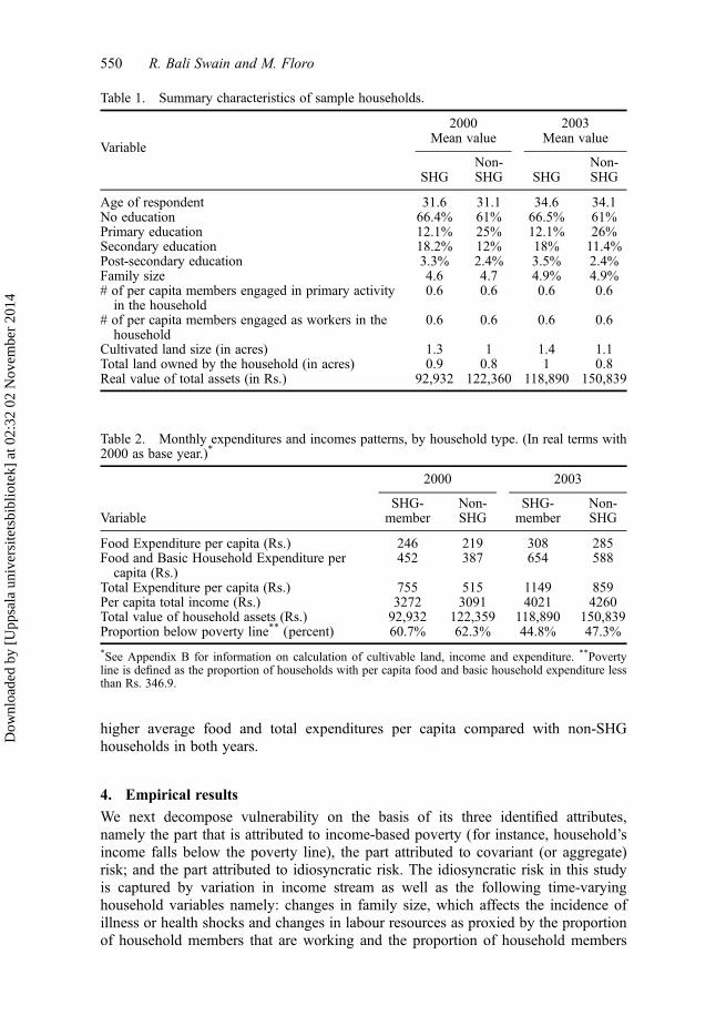
Nabard’s choice to expand the SHG program occurs at the district level withoutany specific policy targeting certain villages over others (Bali Swain and Varghese2009). Thus, we choose to sample at the district level, the basic administrative unitwithin a state. The sampling strategy randomly chose 858 respondents from theSHG members at the district level. The non-members (167 respondents) were chosento reflect a comparable socio-economic group as the SHG respondents. Although theSHGs tend to target poorer households, the program does not follow strict eligibilitycriteria. The quality of the match between the SHG and non-SHG members withinour sample is reflected in Table 1. In the year 2000, the SHG members and non-members are quite alike. On average they are about 31.5 years old and more thantwo-thirds of them are illiterate. Other household characteristics such as family size,number of household members engaged in primary activity and working, are verysimilar. On average SHG and non-SHG members own and cultivate plots of about 1acre. In terms of their real value of total assets, on average non-SHG members arewealthier than the SHG members.

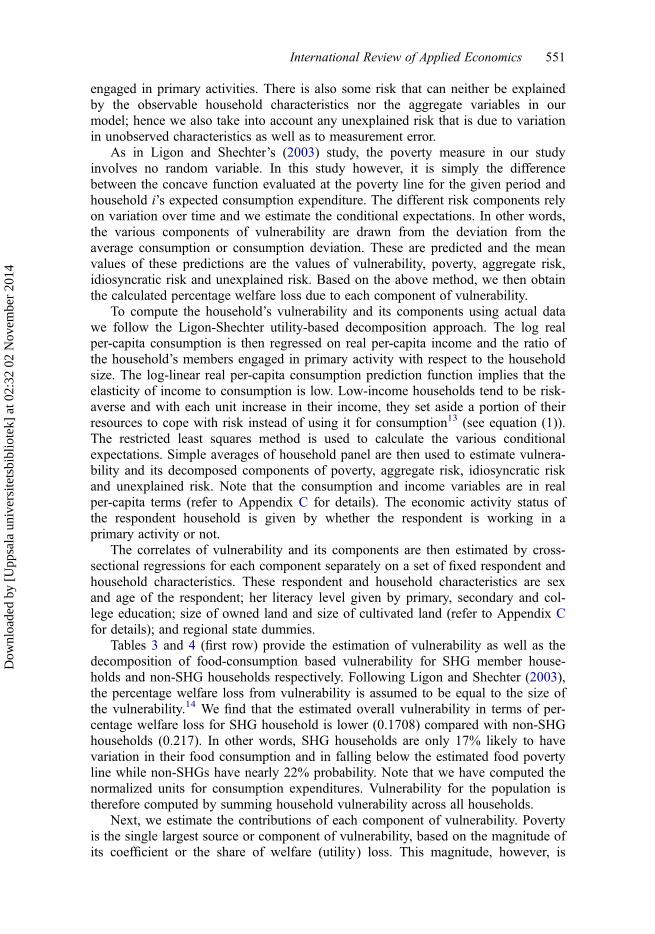
Table 2 presents the monthly expenditures and incomes of the SHG memberhouseholds (treatment group) and the non-SHG households (control group) in realterms. That is, we adjusted the 2003 values using the rural CPI index of India with2000 as the base year. On average about 48.7% (52.5%) of the total expenditure in2003 (2000) was on food. Adding the household expenditure to food, this figurerises to 81.5% (82.7%) of the total expenditure in 2003 (2000). This high percentageof basic expenditure (without even taking the expenditures related to housing (ifany), electricity, water etc. into account) shows that the majority of the householdsin rural areas are very close to poverty if not below the poverty line. Although SHGhouseholds have lower wealth compared with non-SHG households, the former have


Dow

nloa

ded

by [

Upp

sala

uni

vers

itets

bibl

iote

k] a

t 02:

32 0

2 N

ovem

ber

2014

higher average food and total expenditures per capita compared with non-SHGhouseholds in both years.

4. Empirical results

We next decompose vulnerability on the basis of its three identified attributes,namely the part that is attributed to income-based poverty (for instance, household’sincome falls below the poverty line), the part attributed to covariant (or aggregate)risk; and the part attributed to idiosyncratic risk. The idiosyncratic risk in this studyis captured by variation in income stream as well as the following time-varyinghousehold variables namely: changes in family size, which affects the incidence ofillness or health shocks and changes in labour resources as proxied by the proportionof household members that are working and the proportion of household members

Table 1. Summary characteristics of sample households.

2000 2003

VariableMean value Mean value

SHGNon-SHG SHG

Non-SHG

Age of respondent 31.6 31.1 34.6 34.1No education 66.4% 61% 66.5% 61%Primary education 12.1% 25% 12.1% 26%Secondary education 18.2% 12% 18% 11.4%Post-secondary education 3.3% 2.4% 3.5% 2.4%Family size 4.6 4.7 4.9% 4.9%# of per capita members engaged in primary activityin the household

0.6 0.6 0.6 0.6

# of per capita members engaged as workers in thehousehold

0.6 0.6 0.6 0.6

Cultivated land size (in acres) 1.3 1 1.4 1.1Total land owned by the household (in acres) 0.9 0.8 1 0.8Real value of total assets (in Rs.) 92,932 122,360 118,890 150,839

Table 2. Monthly expenditures and incomes patterns, by household type. (In real terms with2000 as base year.)*

2000 2003

VariableSHG-member

Non-SHG

SHG-member

Non-SHG

Food Expenditure per capita (Rs.) 246 219 308 285Food and Basic Household Expenditure percapita (Rs.)

452 387 654 588

Total Expenditure per capita (Rs.) 755 515 1149 859Per capita total income (Rs.) 3272 3091 4021 4260Total value of household assets (Rs.) 92,932 122,359 118,890 150,839Proportion below poverty line** (percent) 60.7% 62.3% 44.8% 47.3%

*See Appendix B for information on calculation of cultivable land, income and expenditure. **Povertyline is defined as the proportion of households with per capita food and basic household expenditure lessthan Rs. 346.9.


Dow

nloa

ded

by [

Upp

sala

uni

vers

itets

bibl

iote

k] a

t 02:

32 0

2 N

ovem

ber

2014

engaged in primary activities. There is also some risk that can neither be explainedby the observable household characteristics nor the aggregate variables in ourmodel; hence we also take into account any unexplained risk that is due to variationin unobserved characteristics as well as to measurement error.

As in Ligon and Shechter’s (2003) study, the poverty measure in our studyinvolves no random variable. In this study however, it is simply the differencebetween the concave function evaluated at the poverty line for the given period andhousehold i’s expected consumption expenditure. The different risk components relyon variation over time and we estimate the conditional expectations. In other words,the various components of vulnerability are drawn from the deviation from theaverage consumption or consumption deviation. These are predicted and the meanvalues of these predictions are the values of vulnerability, poverty, aggregate risk,idiosyncratic risk and unexplained risk. Based on the above method, we then obtainthe calculated percentage welfare loss due to each component of vulnerability.

To compute the household’s vulnerability and its components using actual datawe follow the Ligon-Shechter utility-based decomposition approach. The log realper-capita consumption is then regressed on real per-capita income and the ratio ofthe household’s members engaged in primary activity with respect to the householdsize. The log-linear real per-capita consumption prediction function implies that theelasticity of income to consumption is low. Low-income households tend to be risk-averse and with each unit increase in their income, they set aside a portion of theirresources to cope with risk instead of using it for consumption13 (see equation (1)).The restricted least squares method is used to calculate the various conditionalexpectations. Simple averages of household panel are then used to estimate vulnera-bility and its decomposed components of poverty, aggregate risk, idiosyncratic riskand unexplained risk. Note that the consumption and income variables are in realper-capita terms (refer to Appendix C for details). The economic activity status ofthe respondent household is given by whether the respondent is working in aprimary activity or not.

The correlates of vulnerability and its components are then estimated by cross-sectional regressions for each component separately on a set of fixed respondent andhousehold characteristics. These respondent and household characteristics are sexand age of the respondent; her literacy level given by primary, secondary and col-lege education; size of owned land and size of cultivated land (refer to Appendix Cfor details); and regional state dummies.

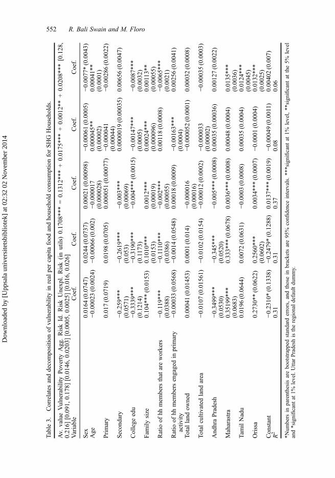
Tables 3 and 4 (first row) provide the estimation of vulnerability as well as thedecomposition of food-consumption based vulnerability for SHG member house-holds and non-SHG households respectively. Following Ligon and Shechter (2003),the percentage welfare loss from vulnerability is assumed to be equal to the size ofthe vulnerability.14 We find that the estimated overall vulnerability in terms of per-centage welfare loss for SHG household is lower (0.1708) compared with non-SHGhouseholds (0.217). In other words, SHG households are only 17% likely to havevariation in their food consumption and in falling below the estimated food povertyline while non-SHGs have nearly 22% probability. Note that we have computed thenormalized units for consumption expenditures. Vulnerability for the population istherefore computed by summing household vulnerability across all households.

Next, we estimate the contributions of each component of vulnerability. Povertyis the single largest source or component of vulnerability, based on the magnitude ofits coefficient or the share of welfare (utility) loss. This magnitude, however, is


Dow

nloa

ded

by [

Upp

sala

uni

vers

itets

bibl

iote

k] a

t 02:

32 0

2 N

ovem

ber

2014

Table

3.Correlatesanddecompositio

nof

vulnerability

inreal

percapita

food

andhouseholdconsum

ptionforSHG

Households.

Av.

valueVulnerabilityPoverty

Agg.RiskId.RiskUnexpl.Risk(inutils)0.1708***=0.1312***+0.0175***+0.0012**

+0.0208***[0.128,

0.216]

[0.091,0.178]

[0.0146,

0.0203][0.0005,

0.0025][0.016,0.026]

Variable

Coef.

Coef.

Coef.

Coef.

Coef.

Sex

0.0164

(0.0747)

0.0244

(0.0737)

0.00021(0.00098)

−0.00061(0.0005)

−0.0077*(0.0043)

Age

−0.00023(0.0024)

−0.00066(0.002)

−0.000017

(0.000028)

0.000045**

(0.00002)

0.00041**

(0.0001)

Primary

0.017(0.0719)

0.0198

(0.0705)

0.000051

(0.00077)

−0.000041

(0.00044)

−0.00286(0.0022)

Secondary

−0.259***

(0.0571)

−0.2619***

(0.053)

−0.003***

(0.00069)

0.0000019(0.00035)

0.00656(0.0047)

College

edu

−0.3339***

(0.1214)

−0.3190***

(0.1173)

−0.004***

(0.0015)

−0.00147***

(0.0005)

−0.0087***

(0.0032)

Fam

ilysize

0.104***

(0.0153)

0.1010***

(0.0153)

0.0012***

(0.00019)

0.00024***

(0.000096)

0.00113**

(0.00055)

Ratio

ofhh

mem

bers

that

areworkers

−0.119***

(0.0388)

−0.1110***

(0.0386)

−0.002***

(0.00055)

0.00118(0.0008)

−0.0065***

(0.0021)

Ratio

ofhh

mem

bers

engagedin

prim

ary

activ

ity−0.00033(0.0568)

−0.0014

(0.0548)

0.00018(0.0009)

−0.00163***

(0.0004)

0.00256(0.0041)

Total

land

owned

0.00041(0.01453)

0.0001

(0.014)

−0.000016

(0.00016)

−0.000052

(0.0001)

0.00032(0.0008)

Total

cultivatedland

area

−0.0107

(0.01561)

−0.0102

(0.0154)

−0.00012(0.0002)

−0.000033

(0.00002)

−0.00035(0.0003)

AndhraPradesh

−0.3499***

(0.0530)

−0.345***

(0.0520)

−0.005***

(0.0008)

0.00035(0.00036)

0.00127(0.0022)

Maharastra

0.35199***

(0.0683)

0.333***

(0.0678)

0.0036***(0.0008)

0.00048(0.0004)

0.0135***

(0.0036)

Tam

ilNadu

0.0196

(0.0644)

0.0072

(0.0631)

−0.0003

(0.0008)

0.00035(0.0004)

0.0124***

(0.0045)

Orissa

0.2730**

(0.0622)

0.2560***

(0.0602)

0.0034***(0.0007)

−0.0001

(0.0004)

0.0132***

(0.0025)

Constant

−0.2310*(0.1338)

−0.2479*(0.1288)

0.0137***(0.0019)

−0.00049(0.0011)

0.00402(0.007)

R2

0.31

0.31

0.37

0.08

0.06

*Num

bers

inparenthesisarebo

otstrapp

edstandard

errors,andthosein

brackets

are95

%confi

denceintervals.

***significant

at1%

level,**

sign

ificant

atthe5%

level

and*significant

at1%

level.UttarPradesh

istheregion

aldefaultdu

mmy.


Dow

nloa

ded

by [

Upp

sala

uni

vers

itets

bibl

iote

k] a

t 02:

32 0

2 N

ovem

ber

2014

Table

4.Correlatesanddecompositio

nof

vulnerability

inreal

percapita

food

andhouseholdconsum

ptionforNON-SHG

households.

Av.

valueVulnerabilityPoverty

Agg.RiskId.RiskUnexpl.Risk(inutils)0.217***

=0.175***

+0.019***

+0.0015

+0.022***

[0.126,0.326]

[0.0817,

0.28][0.013,0.026]

[0.00012,0.0048][0.0141,

0.0319]

Variable

Coef.

Coef.

Coef.

Coef.

Coef.

Sex

−0.202(0.2244)

−0.208(0.2153)

−0.0028

(0.0024)

0.000047

(0.0027)

0.00851(0.0086)

Age

−0.0105**

(0.0045)

−0.010**(0.0045)

−0.0001*

(0.00006)

0.000019

(0.00008)

−0.000075

(0.0004)

Primary

0.0984

(0.1196)

0.0961

(0.1136)

0.0016

(0.0017)

−0.0004

(0.00092)

0.001(0.0067)

Secondary

−0.0134

(0.1185)

−0.006(0.1151)

0.000054

(0.0016)

−0.0002

(0.0016)

−0.006(0.0062)

College

edu

−0.560**(0.2613)

−0.538**(0.2585)

−0.0085**

(0.0035)

−0.0034**

(0.0016)

−0.009(0.0108)

Fam

ilysize

0.115***

(0.0367)

0.1129***

(0.0352)

0.0012**

(0.0005)

−0.0001

(0.0004)

0.001(0.0019)

Ratio

ofhh

mem

bers

that

areworkers

−0.017(0.2183)

−0.0206

(0.2120)

−0.0004

(0.0027)

−0.0002

(0.0027)

0.003(0.0087)

Ratio

ofhh

mem

bers

engagedin

prim

ary

activ

ity−0.197(0.2275)

−0.1829

(0.2285)

−0.0032

(0.0028)

−0.003***

(0.0015)

−0.007(0.0066)

Total

land

owned

−0.064(0.0920)

−0.0623

(0.0919)

−0.0007

(0.0011)

−0.000073

(0.0007)

−0.001(0.0037)

Total

cultivatedland

area

0.007(0.0788)

0.0068

(0.0771)

0.0001

(0.0009)

0.000044

(0.0007)

0.0003

(0.0043)

AndhraPradesh

−0.529***

(0.1285)

−0.523***

(0.1265)

−0.008***

(0.0019)

−0.001(0.0015)

0.002(0.013)

Maharastra

0.061(0.1214)

0.0531

(0.1657)

0.0003

(0.0019)

−0.0004

(0.0018)

0.008(0.0085)

Tam

ilNadu

−0.202*

(0.1214)

−0.199(0.1216)

−0.0036**

(0.0015)

−0.0019*(0.0011)

0.001(0.0077)

Orissa

0.284**(0.1372)

0.270***

(0.1341)

0.0031*(0.0017)

−0.0003

(0.0020)

0.01

(0.0091)

Constant

0.404(0.3346)

0.367(0.3280)

0.0227***

(0.0057)

0.0051

(0.0065)

0.009(0.0195)

R2

0.35

0.34

0.40

0.13

0.04

*Num

bers

inparenthesisarebo

otstrapp

edstandard

errors,andthosein

brackets

are95

%confi

denceintervals.

***significant

at1%

level,**

sign

ificant

atthe5%

level

and*significant

at1%

level.UttarPradesh

istheregion

aldefaultdu

mmy.


Dow

nloa

ded

by [

Upp

sala

uni

vers

itets

bibl

iote

k] a

t 02:

32 0

2 N

ovem

ber

2014

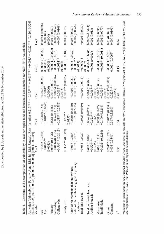
higher in the case of non-SHG households (0.175) compared with 0.1312 of SHGhouseholds. This implies that an important effect of SHG on vulnerability is its con-tribution in terms of its income (poverty reduction) effect among SHG householdsvia increased access to credit (or at better terms) as well as to training. In terms ofthe risk components, unexplained risk (as well as measurement error) is the largestpart in both SHG and non-SHG models (Tables 3 and 4), followed closely by theaggregate risk as shown in Tables 3 and 4. However, we note that the difference inthe coefficients on aggregate risk between SHG households (0.0175) and non-SHGhouseholds (0.019) is smaller.

The explained idiosyncratic risk in both Tables 3 and 4 is quite small (0.0012and 0.0015), suggesting that the unobserved idiosyncratic shocks or variations inhousehold attributes may be embedded in the unexplained risk. Overall, our resultsshow that the non-pecuniary effect of SHG on the vulnerability of the household interms of its ability to cope with idiosyncratic risk is not as strong as its directincome effect.

We next look at the correlates of these vulnerability components. The regressionresults in Tables 3 and 4 uses the following fixed characteristics namely sex, educa-tion and age of respondent as well as some state dummy variables. It can be notedthat an increase in education from none to primary level of the respondents does notyield any significant impact on vulnerability nor on any of its components. Amongthe SHG households however, secondary education, on average, significantlyreduces (25%) the vulnerability of households compared with households where therespondent is uneducated. Among non-SHG households, it is only when the respon-dent has at least college education is the household significantly (56%) less vulnera-ble compared with a household where the respondent is uneducated. Much of thisreduction is due to educated households having higher expected incomes, and to asmaller degree, due to significantly less exposure to aggregate and idiosyncratic risk.For both SHG and non-SHG households, vulnerability increases significantly withfamily size by 10%. Interestingly, we find that the smaller the number of workersamong SHG households, the more (11%) vulnerable is the household. This isbecause more workers per household significantly increases the expected householdearnings and hence reduces poverty.

Our results also suggest that wealth proxy variables in the form of total ownedlandholding and total cultivated land do not seem to affect the vulnerability of thehousehold or the level of risk. This could be due to the fact that most of the SHGborrowers and control households in the sample own or cultivate very small landareas for subsistence purposes. Given their heavy reliance on traditional productionmethods and rainfall (or weather) dependence, the size of land they operate may beinadequate to protect them from risk and poverty.

Finally, we find that SHG households living in Andhra Pradesh are likely to be34% less vulnerable compared with Uttar Pradesh. While those living in Maharastraand Orissa are likely to be 35% and 27% respectively more vulnerable (see Table 3).Among non-SHG households, we find that those living in Andhra Pradesh andTamil Nadu are likely to be 53% and 20% less vulnerable respectively comparedwith Uttar Pradesh, while those living in Orissa are likely to be 28% more vulnera-ble. These differences reflect the higher level of economic development and SHGprogram development in the southern states of Andhra Pradesh and Tamil Nadu,compared with the south-eastern state of Orissa, which is relatively morebackward.15


Dow

nloa

ded

by [

Upp

sala

uni

vers

itets

bibl

iote

k] a

t 02:

32 0

2 N

ovem

ber

2014

Overall, our tests results show that poverty is the most significant component ofvulnerability among our rural household sample, whereas aggregate risk andunexplained risk show a much lower contribution. The idiosyncratic component isrelatively minuscule. These findings imply that being poor (based on the foodconsumption poverty measure), by itself, is the main contributor to vulnerability.

5. Concluding remarks

This paper explores an important dimension of household welfare that conventionalmeasures of poverty do not address, namely the ability of households to cope withrisks, idiosyncratic as well as aggregate or covariant. In particular, we want to under-stand the realities pertaining to the economic situation of rural low-income house-holds by exploring the determinants of vulnerability. We also examine the likelyeffect of self-help microfinance groups on vulnerability using an Indian householdsurvey panel data for 2000 and 2003 by comparing treatment or SHG memberhouseholds with control or non-SHG households.

We then develop a theoretical model that explains the risk-coping mechanismthrough which SHG participation may result in the member-household’s decliningvulnerability. We take into account the varied sources of vulnerability in order tobetter understand the impact of self-help microfinance groups on the economic situa-tion of women in rural households. Our construction of the vulnerability measuredraws from the work of Ligon and Schechter (2003). Their measure of vulnerabilityallows for the quantification of the welfare loss associated with poverty as well fromaggregate and idiosyncratic risks that expose households to consumption shocks.The decomposition method enables us to capture the effects of risk on the house-hold’s agency or welfare. Hence, we are able to assess the likely impact of self-helpmicrofinance groups via the income effect (through access to credit, savings andtraining services) and non-pecuniary effect on aggregate or idiosyncratic risk. Usingthe data from SHG and non-SHG households in India, our empirical tests show thatSHG’s microfinance program respondents are less vulnerable compared with thenon-SHG respondents (control group). Our estimates in Table 5 suggest that foodconsumption-based poverty still remains the largest component of SHGs’ (76.8%)vulnerability as well as the non-SHG households’ (80.6%) vulnerability. The idio-syncratic risk that results from observable sources (such as income shocks and theirbeing not engaged in any economic activity), are insignificant in terms of magnitudeand statistical significance. This may be due to the fact that our panel contains infor-mation on only two time periods and to the limitations of the recall method used inthe survey.

Table 5. Percentage contribution to the total vulnerability for model (in per cent).

SHG Households Non-SHG households

Poverty component of vulnerability 76.8 80.6Aggregate risk 10.2 8.7Idiosyncratic risk 0.7 0.7Unexplained risk 12.1 10.1


Dow

nloa

ded

by [

Upp

sala

uni

vers

itets

bibl

iote

k] a

t 02:

32 0

2 N

ovem

ber

2014

Our study of vulnerability suggests that poverty is the most significant source ofvulnerability among our rural household sample. These findings imply that beingpoor is, by itself, the main contributor to vulnerability. Moreover, we find that SHGparticipation tends to reduce the vulnerability of households, largely through itsimpact on poverty reduction, and to a much smaller extent, its non-pecuniary effecton risk. The limited non-pecuniary impact of self-help microfinance groups on therisk component of vulnerability suggests that such impacts might take effect over amuch longer time period than our data captures.

Notes1. For a detailed discussion on SHG refer to Bali Swain (2012).2. In the literature on risk and poverty, there is a distinction made between precautionary

strategies towards risk and ex post strategies after a shock or economic crisis. Both exante strategies (precautionary) and ex post strategies (managing a loss) for dealing withrisk involve a mix of intra-household measures (self-insurance) and inter-householdmeasures (informal and formal insurance).

3. Surveys of this literature are in Townsend (1995), Bardhan and Udry 1999; Dercon2005; Zimmerman and Carter 2003, Deaton (1997), Morduch (2004).

4. Recent studies including Ligon and Schechter (2003) have used some variant of the“expected utility” function as the basis for measuring vulnerability.

5. The model presented here follows the work by Leland (1968) and Sandmo (1970).6. Our study focuses more on the notion of household welfare rather than on household

utility. While the latter is defined as an abstract measure of satisfaction, welfare isdefined as the physical, social, and mental development of human capabilities obtainedby means of access to and consumption of basic commodities (such as food, health care,education, and shelter), participation in activities. For a more detailed discussion of thistopic, see Floro (1995). Although there are obvious links between economic welfareand utility, they are not necessarily closely connected.

7. The idea here is similar to the risk coping behaviour addressed in Townsend (1995),Sebstad and Cohen (2001), Bardhan and Udry (1999), Dercon and Krishnan (2000) andEllis (1998) to name a few.

8. Vulnerability is treated here as a subjective perception based on the household’s experi-ence of both aggregate and idiosyncratic shocks, their resources (social and financial)when shock occurs, as well as the household’s perception about its future income flows.

9. Ligon and Schecter (2003) estimated the distribution of future consumption expendi-tures for every household using a 12-month time period panel Bulgarian householdsurvey.

10. The log-linear consumption prediction function is chosen since employing expenditurelevels in a linear prediction equation may sometimes predict negative levels of con-sumption (Ligon and Schechter 2004).

11. The process involved discussion with statisticians, economists and practitioners at thestage of sampling design, preparing pre-coded questionnaires, translation and pilot test-ing with at least 20 households in each of the five states (100 households in total). Thequestionnaires were then revised, reprinted and the data collected by local surveyorsthat were trained and supervised by the supervisors. The standard checks were appliedboth on the field and during the data punching process.

12. These states (districts in parentheses) are Orissa (Koraput and Rayagada), AndhraPradesh (Medak and Warangal), Tamil Nadu (Dharamapuri and Villupuram), UttarPradesh (Allahabad and Rae Bareli), and Maharashtra (Gadchiroli and Chandrapur).

13. Even though Ligon and Schechter (2003) use a linear function, in their 2004 paper theyuse the log-linear consumption prediction function.

14. Note that the manner in which utility (or welfare) function is defined in their study, theutility (or welfare) from perfect equality (i.e. steady or uniform consumption level) in ariskless society is equal to 1.


Dow

nloa

ded

by [

Upp

sala

uni

vers

itets

bibl

iote

k] a

t 02:

32 0

2 N

ovem

ber

2014

15. Andhra Pradesh and Tamil Nadu accounted for 48.5% and 12.5% of the cumulativenumber of SHGs provided with bank loans up to 2002. They were followed by UttarPradesh (7%), Orissa (4.1%) and Maharashtra (4%).

16. The Task Force on the ‘Projections of Minimum Needs and Effective ConsumptionDemands’ (1979) defines the poverty line (BPL) as the cost of an all India average con-sumption basket that meets the calorie norm of 2400 calories per capita per day forrural areas and 2100 for the urban areas. These calorie norms are expressed in monetaryterms as Rs. 49.09 and Rs. 56.64 per capita per month for rural and urban areas respec-tively at 1973–74 prices. Based on the recommendations of a study group on ‘The Con-cept and Estimation of Poverty Line’, the private consumption deflators from nationalaccounts statistics was selected to update the poverty lines in 1977–78, 1983 and 1987–88. Subsequently, the expert group under the Chairmanship of late Professor D.T.Lakdawala recommended the use of consumer price index for agricultural labour toupdate the rural poverty line and a simple average of weighted commodity indices ofthe consumer price index for industrial workers and for urban non-manual employees toupdate the urban poverty line. But the Planning Commission accepted only the CPI forindustrial workers to estimate and update the urban poverty line (Economic Survey ofDelhi, 2001–2002).

17. Calculation of poverty only on the basis of calorie consumption is inadequate and mostresearchers would agree with this (including us).

18. I chose November 2003 because most of our data is collected in that month in 2003.19. This was calculated as the average of the CPI for Agricultural laborers at base 1986–

87, over the period July 2004 to June 2005 = (1/12)(338 + 341 + 343 + 345 + 344 +342 + 341 + 340 + 340 + 341 + 343 + 345).

ReferencesAckerly, B. 1997. “What’s in a Design the Effects of NGO Programme Delivery Choices on

Women’s Empowerment in Bangladesh.” In Getting Institutions Right for Women inDevelopment, edited by Anne Marie Goetz, 140–160. London and New York: ZedBooks.

Amin, S., A. S. Rai and G. Topa. 1999. “Does Microcredit Reach the Poor and Vulnerable?Evidence from Northern Bangladesh.” Working paper 28, Centre for International Devel-opment at Harvard University.

Armendariz, B., and J. Morduch. 2010. The Economics of Microfinance. 2nd ed. Cambridge,Mass: MIT Press.

Bali Swain, R. 2007. “Impacting Women through Microfinance.” Dialogue, Appui Au Dével-oppement Autonome 37: 61–82.

Bali Swain, R., and A. Varghese. 2009. “Does Self Help Group Participation Lead to AssetCreation?” World Development 37 (10): 1674–1682.

Bali Swain, R., and F. Y. Wallentin. 2009. “Does Microfinance Empower Women?” Interna-tional Review of Applied Economics 23 (5): 541–556.

Bali Swain, R. 2012. The Microfinance Impact. Oxon and New York: Routledge.Bali Swain, R., and M. Floro. 2012. “Assessing the Effect of Microfinance on Vulnerability

and Poverty among Low Income Households.” Journal of Development Studies 48 (5):605–618.

Bardhan, P., and C. Udry. 1999. Development Microeconomics. Oxford: Oxford UniversityPress.

Calvo, C., and S. Dercon. 2005. Measuring Individual Vulnerability, Department of Econom-ics Working Paper Series, 229, Oxford University, Oxford.

Carter, M. and M. Ikegami. 2007. “Looking Forward: Theory-based Measures of ChronicPoverty and Vulnerability.” CPRS Working Paper No. 94, University of Wisconsin,Madison.

Christiaensen, L., and K. Subbarao. 2004. “Toward an Understanding of Household Vulnera-bility in Rural Kenya.” World Bank Policy Research Working Paper 3326, World Bank,Washington DC.

De Aghion, B. A., and J. Morduch. 2006. The Economics of Microfinance. Cambridge,Massachusetts: MIT Press.


Dow

nloa

ded

by [

Upp

sala

uni

vers

itets

bibl

iote

k] a

t 02:

32 0

2 N

ovem

ber

2014

Deaton, A. 1997. Analysis of Household Surveys: A Microeconomic Approach to Develop-ment Policy. Washington DC: World Bank.

Dercon, S. 2005. Vulnerability: A Micro Perspective. Mimeo: Oxford University.Dercon, S., and P. Krishnan. 2000. “Vulnerability, Seasonality and Poverty in Ethiopia.”

Journal of Development Studies 36 (6): 25–53.Dichter, T., and M. Harper, eds. 2007. What’s Wrong with Microfinance? Warwickshire:

Practical Action Publishing.Ellis, F. 1998. “Household Strategies and Livelihood Diversification.” The Journal of Devel-

opment Studies 35 (1): 1–38.Floro, M. 1995. “Women’s Well-being, Poverty and Work Intensity.” Feminist Economics

1 (3): 1–25.Ghate, P., S. Gunarajan, V. Mahajan, P. Regy, F. Sinha, and S. Sinha. 2007. Microfinance in

India: A State of the Sector Report. New Delhi: Microfinance India.Glewwe, P., and G. Hall. 1998. “Are Some Groups More Vulnerable to Macroeconomic

Shocks? Hypothesis Tests Based on Panel Data from Peru.” Journal of DevelopmentEconomics 56 (1): 181–206.

Goetz, A. M. 1997. “Introduction.” In Getting Institutions Right for Women in Development,edited by A. M. Goetz, 1–30. London and New York: Zed Books.

Karlan, D. 2007. “Impact Evaluation for Microfinance: Review of Methodological Issues.Poverty Reduction and Economic Management (PREM), Doing Impact Evaluation.”Discussion Paper 7, World Bank, Washington DC.

Leland, H. 1968. “Saving and Uncertainty: The Precautionary Demand for Saving.” Quar-terly Journal of Economics 82: 465–473.

Ligon, E. and L. Schechter. 2002. “Measuring Vulnerability: The director’s Cut.” UN/WIDER Working Paper.

Ligon, E., and L. Schechter. 2003. “Measuring Vulnerability.” The Economic Journal 113(486): 95–102.

Ligon, E. and L. Schechter. 2004. “Evaluating Different Approaches to Estimating Vulnera-bility.” Social Protection Discussion Paper 0210, World Bank, Washington D.C.

Little, I. M. D., and V. J. Joshi. 1994. India: Macroeconomics and Political Economy,1964–1991. Washington, DC: World Bank.

Mayoux, L. 2002. “Women’s Empowerment or Feminisation of Debt? Towards a NewAgenda in African Micro-finance.” Discussion Paper, One World Action Conference,London.

Morduch, J. 1999. “The Microfinance Promise.” Journal of Economic Literature 37: 1569–1614.

Morduch, J. 2004. “Consumption Smoothing across Space: Testing Theories of Risk-Sharingin the ICRISAT Study Region of South India.” In Insurance against Poverty, edited byStefan Dercon, 53–71. Oxford University Press.

NABARD. 2006. “Progress of SHG-bank Linkage in India: 2005–06.” Working Paper,NABARD.

Pitt, M., and S. R. Khandker. 1998. “The Impact of Group-Based Credit Programs on PoorHouseholds in Bangladesh: Does the Gender of Participants Matter?” The Journal ofPolitical Economy 106: 958–996.

Puhazhendi, V., and K. C. Badatya. 2002. SHG-Bank Linkage Programme for Rural Poor –an Impact Assessment, Paper, National Bank for Agriculture and Rural Development–NABARD. India: Mumbai.

Rankin, K. 2002. Social Capital Microfinance and the Politics of Development. FeministEconomics, 8 (1): 1–24.

Sandmo, A. 1970. “The Effect of Uncertainty on Saving Decisions.” Review of EconomicStudies 37: 353–360.

Sebstad, J., and M. Cohen. 2001. Microfinance, Risk Management and Poverty, ConsultativeGroup to Assist the Poorest. Washington DC: The World Bank.

Sen, K., and R. R. Vaidya. 1997. The Process of Financial Liberalization in India. Delhi:Oxford University Press, India.

Srinivasan, N. 2010. Microfinance in India, State of Sector Report. New Delhi: SAGE.Srinivasan, N. 2011. Microfinance in India, State of Sector Report. New Delhi: SAGE.


Dow

nloa

ded

by [

Upp

sala

uni

vers

itets

bibl

iote

k] a

t 02:

32 0

2 N

ovem

ber

2014

Townsend, R. M. 1995. “Consumption Insurance: An Evaluation of Risk-bearing Systems inLow-Income Economies.” Journal of Economic Perspectives 9: 83–102.

World Bank. 2000. India: Reducing Poverty, Accelerating Development. Delhi, Oxford:Oxford University Press.

Zimmerman, F., and M. Carter. 2003. “Asset Smoothing, Consumption Smoothing and theReproduction of Inequality under Risk and Subsistence Constraints.” Journal of Develop-ment Economics 71: 233–260.

Appendix A. Mathematical proofThis appendix provides the mathematical proof of equation (15). The differential of the per-ceived risk function is:

d�U22

U2

� �¼ @

@c1

�U22

U2

� �dc1 þ @

@c2

�U22

U2

� �dc2:

This is negative if c2 increases as c1 decreases, e.g., so that from equation (5) in the text

dc2 ¼ 1ð1þ rÞdc1; ð1þ rÞ� 0:

Substituting for dc1, and dividing by dc2, we then have:

d

dc2

�U22

U2

� �¼ �@

@c1

�U22

U2

� �þ 1þ rð Þ @

@c2

�U22

U2

� �� 0:

We now observe that under the continuity assumption, the following holds as an identity:

@

dc1

�U22

U2

� �¼ @

@c2

�U12

U2

� �:

The above inequality can now be written as:

@

@c2

U12 � 1þ rð ÞU22

U2

� �\0:

We now wish to prove that the increased perceived risk hypothesis implies that thederivative of equation (14) in the text is negative. We first define

c2 ¼ ½ðY1 � c1Þð1þ rÞ� þ n

From equation (5), we know that:

c2 ¼ c2 þ Y2 � n:

Because [U12 – (1 + σ) U22 ] / U2 is decreasing in c2, we must have that

U12 � 1þ rð ÞU22

U2

� �� U12 � 1þ rð ÞU22

U2

� �ifY2 � n: (E.1)

Note that the right-hand side of this inequality is evaluated at c2 ¼ c2 and is not a ran-dom variable. This implies that:

U2(Y2 – ξ) ≤ 0 if Y2 ≥ ξ.

Multiplying both sides of equation (E.1) by U2(Y2 – ξ), we obtain the following:

U12 � ð1þ rÞU22½ �f ðY2 � nÞg� U12 � ð1þ rÞU22

U2

� �� UðY2 � nÞ½ � (E.2)


Dow

nloa

ded

by [

Upp

sala

uni

vers

itets

bibl

iote

k] a

t 02:

32 0

2 N

ovem

ber

2014

if Y2 ≥ ξ. Given this, the inequalities in equations (E.1) and (E.2) will be reversed so thatthe expected values hold for all Y2.

E U12 � ð1þ rÞU22½ �ððY2 � nÞ� U12 � ð1þ rÞU22

U2

� �n

�E U2ðY2 � nÞ½ �: (E.3)

To prove that the left side of (E.3) is negative, it is sufficient to show that the right side isnegative. From equation (10) in the text, the expression in braces is positive so that we haveto show that E UðY2 � nÞ½ � � 0: Since U22 < 0, we must have

U2 �ðU2Þn ifY2 � n (E.4)

Multiplying equation (E.4) by (Y2 –ξ), we can write

U2 �ðU2Þnh i

ðY2 � nÞifY2 � n (E.5)

This holds for all Y2, since inequalities in equation (E.4) are reversed if Y2 ≤ ξ.Taking the expected values, we then obtain

E U2ðY2 � nÞ½ � � ðU2ÞEðY2 � nÞ ¼ 0

which implies

E U12 � ð1þ rÞU22½ �ðY2 � nÞ� 0: (E.6)

Therefore, since D < 0, it follows that equation (14):

ð@c1@c

Þ ¼ �ð 1D2

ÞE U12 � ð1þ rÞU22½ �f ðY2 � nÞg (E.7)

is negative. Hence,@R1

@c[ 0: Q.E.D.

Appendix B. Estimation of poverty line-based Z variableThe poverty line is an important part of the analysis and our results are sensitive to the typeof poverty line measure used. The World Bank defines the poverty line as US$1 per personper day. However, if this definition of poverty is to be used, according to one estimate about75% of Indian households would be below the poverty line for 2000–2001. India’s officialpoverty rate given for that year is 26%.

The official poverty line estimations in India are based on the norm of 2400 calories percapita per day for rural areas and 2100 per capita per day for the urban areas.16 These pov-erty estimates are derived from the household consumer expenditure data collected byNational Sample Survey Organisation (NSSO) of the Ministry of Statistics and ProgrammeImplementation, every fifth year. Using the survey and the methodology of the PlanningCommission, the Government of India, has released the poverty estimates for the years1973–74, 1977–78, 1983, 1987–88, 1993–94 and 1999–2000, released on 22 February 2001.The NSSO also conducts Annual household consumer expenditure surveys but the samplesize is much smaller for them, therefore the Planning Commission does not take these annualsurveys into account for estimating poverty.

According to the ‘Household Consumption Expenditure in India 1999-2000’, ‘NSS 55thRound, Report No. 454’ and ‘Nutritional Intake in India 1999-2000’, ‘NSS 55th Round,Report No. 471’, the rural estimate for the poverty line is 327.5 rupees for All India.According to the 61st round of the NSS covering period July 2004 to June 2005, the esti-mated Poverty Line in 2004–2005 is Rs. 356.3. per capita per month (see Poverty Estimatesfor 2004–2005, Government of India, Press Information Bureau, March 2007). The correct


Dow

nloa

ded

by [

Upp

sala

uni

vers

itets

bibl

iote

k] a

t 02:

32 0

2 N

ovem

ber

2014

way would be to deflate the 2004–2005 poverty line based on the CPI for agriculturallabourers for rural areas.17 Hence the relevant poverty line for November 2003 wascalculated as follows:

(A) Official All-India Poverty Line estimate for 2003 = Rs. 356.30(B) CPI for agri. Labourers (at base prices 1986-87) for November 200318 = 333(C) CPI for July 2004 to June 200519 = 342

Poverty Line Estimate for November 2003 is then calculated asA * (B / C) = (356.3) * (333 / 342) = Rs.346.9

Appendix CCalculation of the net income of the householdThe net income of the household for 2003 and 2000 was calculated separately as the sum of:wage employment of all the members of the household (in cash and kind); net income of allmembers from own-farm (revenue minus production and hiring cost); net income of all mem-bers engaged in self-employed activity; household income from livestock; and wage employ-ment in non-farm activity.

Calculation of food expenditureThe total food expenditure for 2000 and 2003 was calculated separately as the sum of theexpenditure on staple grains; fruits and vegetables; meat/chicken/fish and dairy products;cooking oil; fuel, coal or kerosene oil; sugar, spices, tea and biscuits; plus other miscella-neous food items.

Other household expenditure includes spending on children and adult clothing and footwear;soaps, washing powder and cosmetics; kitchen and other goods.

Total cultivated area is the sum of the total amount of land owned plus the net amount ofland leased-in for cultivation

The figures for the expenditure, income and total value of household assets for the year2000 have been inflated using the state-level Consumer Price Index for Agricultural labourersbased on the 1986–87 for the months of November 2003 and July 2000. The source for theJuly 2000 figures is the Annual Report of CPI (agricultural and rural labourers) 2002–2003,Government of India. For the November 2003 figures the source was the Annual Report onCPI for agricultural and rural labour for agriculture year 2004–2005. To construct the inflatorthe following formula is used

Inflator = (figure in Rs. for the year 2000) * (CPI for 2003/CPI for 2000) (C1)Using equation (C1) the following inflators were calculated for the five states and used to

inflate the data on expenditure and income for 2000.

Andhra Pradesh 348/325=1.071Uttar Pradesh 330/307=1.075Maharashtra 333/311=1.071Tamil Nadu 350/300=1.167Orissa 320/313=1.022


Dow

nloa

ded

by [

Upp

sala

uni

vers

itets

bibl

iote

k] a

t 02:

32 0

2 N

ovem

ber

2014

microfinance, vulnerability and risk in low income households

Documents