methods to classify bainite in wire rod steel

Methods to Classify Bainite in Wire Rod Steel

Marc Ackermann,* Bernard Resiak, Pascal Buessler, Bertrand Michaut,Jean-Christophe Hell, Silvia Richter, James Gibson, and Wolfgang Bleck

1. Introduction

Bainite is known as probably the most complex microstructure insteel with similarities to other microstructures dependingon the transformation temperature and the alloying concept.

A simplified classification of bainite wasintroduced by Takahashi and Bhadeshiaby differentiating lower from upper bainitebased on the occurrence of intralath orinterlath cementite.[1] However, the devel-opment of alloying concepts and newprocessing routes caused more varietiesin the bainitic microstructure. In need ofa new classification approach, Zajac catego-rized different types of bainite according tothe misorientation angle at the phaseboundary.[2,3] In the last decades, the differ-ent appearances of bainite have caused avast list of terminologies. Bramfitt andSpeer compiled a list of 30 terms extractedfrom various publications, all referring todifferent types of bainite.[4] Since then,the list can be extended by further termsto describe bainite.[5–9] One conclusion ofthe previous work is that the classificationof different bainite microstructuresdepends highly on the expert and thereforecauses ambiguous interpretations.

Another trend that has evolved in recentyears is the increasing application of high-resolution techniques with results reaching

to an atomic level. It is true that high-resolutionmethods (such astransmission electron microscopy (TEM), atom probe tomogra-phy (APT), and atom force microscopy (AFM)) provide usefulinformation at the nanometer scale. But the localized informa-tion cannot always be generalized and applied to the bulk

M. Ackermann, Prof. W. BleckSteel InstituteRWTH Aachen UniversityIntzestr. 1, 52072 Aachen, GermanyE-mail: [email protected]

Dr. B. Resiak, P. Buessler, Dr. B. MichautBars and WiresArcelorMittal Global Research and DevelopmentVoie Romaine BP 30320, 57283 Maizières-Lès-Metz Cedex, France

The ORCID identification number(s) for the author(s) of this articlecan be found under https://doi.org/10.1002/srin.202000454.

© 2020 The Authors. Steel Research International published by Wiley-VCHGmbH. This is an open access article under the terms of the CreativeCommons Attribution License, which permits use, distribution andreproduction in any medium, provided the original work is properly cited.

The copyright line for this article was changed on 17 December 2020 afteroriginal online publication.

DOI: 10.1002/srin.202000454

Dr. J.-C. HellMaizières ProductsArcelorMittal Global Research and DevelopmentVoie Romaine BP 30320, 57283 Maizières-Lès-Metz Cedex, France

Dr. S. RichterCentral Facility for Electron MicroscopyRWTH Aachen UniversityMies-van-der-Rohe-Straße 59, 52074 Aachen, Germany

Dr. J. GibsonInstitute of Physical Metallurgy and Metal PhysicsRWTH Aachen UniversityKopernikusstr. 14, 52074 Aachen, Germany

The microstructural description in bainitic steel is commonly ambiguous, and theinterpretations of results that originate from applied methods are usually userdependent. In consequence, a manifold description of bainite makes it difficult toreveal structure–property relationships. This is why a novel classification andquantification routine for bainitic microstructures in wire rod steel is presented.The classification is based on electron probe microanalysis (EPMA), electronbackscatter diffraction (EBSD), and nanohardness of the same local area.Microstructural constituents with different characteristics (carbon concentration,misorientation, and nanohardness) are classified into low-, intermediate-, andhigh-temperature morphologies. After the classification, quantification is con-ducted by combining scanning electron microscopy (SEM) analysis, dilatometry,and X-ray diffraction (XRD). The bainite quantification reveals a homogeneousmicrostructure for cooling along the lower bainite regime. Increasing themanganese content causes a lower sensitivity to change in the coolingparameters. Combining nanohardness and EBSD is suitable to describemicroscopic microstructural properties, whereas the quantification of bainiteis eligible to explain differences in the microscopic microstructural properties.The used approach avoids overcomplexity and manifold terminologies of bainiticmicrostructures that are commonly found in the literature.

FULL PAPERl

www.steel-research.de

steel research int. 2021, 92, 2000454 2000454 (1 of 12) © 2020 The Authors. Steel Research International published by Wiley-VCH GmbH

mailto:[email protected]

https://doi.org/10.1002/srin.202000454

http://creativecommons.org/licenses/by/4.0/

http://creativecommons.org/licenses/by/4.0/

http://www.steel-research.de

material. For instance, continuous cooled wire rod steel is com-monly exposed to external cooling effects (by air or forced aircooling in a Stelmor conveyor[10]). This causes a temperature gra-dient in the radial direction from the core to the outer surfacedepending on several factors, for example, the wire rod diameterand the ring density on the cooling conveyor.[11] Consequently, amicrostructural and hardness gradient can be observed in thesame direction. In this case, the experimental setup requiresadjustments to deliver more representative results, instead ofrelying only on high-resolution techniques.

In this work, different methods are combined to get a morerepresentative analysis of bainite in wire rod steel. The appliedalloying concept, referred to as carbide-free bainite,[12–14] yieldsan incomplete transformation for the applied cooling parameterswith retained austenite as secondary phase. This alloying conceptis known for an outstanding combination of strength and duc-tility.[5] The retained austenite occurs either as films separatingbainitic lath or as blocks between sheaves of bainite.[15] At roomtemperature, the secondary phase is meta-stable. This means thatexternal events can trigger a transformation of austenite to mar-tensite, known as the transformation-induced plasticity (TRIP)effect.[16] Austenite blocks commonly inherit a carbon gradienttoward the core. Cooling below the Ms temperature partly trans-forms these blocks into martensite, while the outer rim remainsaustenitic to some extent.[13] Therefore, the mixture of martensiteand austenite is commonly referred to as a martensite–austenite(M–A) island.[17]

2. Experimental Section

2.1. Laboratory Melts

In total, three microalloyed steels were produced as laboratorymelts alloyed with substantial differences in manganese content(Table 1). The steels contained a medium carbon content with0.19–0.23 and >1 wt% Si to delay carbide precipitation inaustenite.[18] Manganese of 1.5–2.5 wt% was used to adjust thehardenability.[19] This concept is commonly applied to generate car-bide-free bainite. A combined utilization of boron and titaniumdelays the ferrite/pearlite transformation to widen the process win-dow for bainite.[20] Molybdenum has the same effect with delayingdiffusion-based transformations. In addition, molybdenumimpedesmanganese segregation to the grain boundaries.[21] In con-sequence, grain boundary embrittlement can be avoided. Niobiumwas used to control the grain coarsening during wire hot rolling.

The samples originated from 140� 140 mm2 sized ingotsforged at 1200 �C to billets with a cross-section of60� 60mm2. Samples were cut in the longitudinal directionof the billet with a rectangular geometry of 20� 20� 65mm3,and a second batch of samples with a flat sample geometry of

4� 7� 1.3 mm3 was prepared for dilatometer experiments.The first batch with larger samples was used in a thermomechan-ical treatment simulator (TTS) to apply hot deformation andcooling according to predefined parameters.

2.2. Thermomechanical Treatment

All the samples passed through the same austenitization treat-ment with initial heating of 3 K s�1 to 1200 �C. This temperaturewas held for 10min until cooling with 1 K s�1 to a hot deforma-tion step at 900 �C that initiated compression of the sample(φ¼ 0.3, φ̇¼ 10 s�1). In the following, three different coolingregimes according to the cooling conveyor in a wire rod millwere defined to generate different mixtures of bainite. The cool-ing parameters in regime I consisted of fast initial coolingwith 5 K s�1 to 400 �C and subsequent cooling in the bainitephase field of 0.3 K s�1. Slower cooling of 2 K s�1 from 900 to500 �C with simulated air cooling in the bainite phase field of1 K s�1 is denoted as regime II. Regime III was cooled as regimeII, but the cooling rate in the bainite phase field was reduced to0.3 K s�1. Cooling rates of regimes I–III were confirmed forfeasibility by prior tests on the cooling conveyor of the wirerod mill at ArcelorMittal Duisburg Long Products. A hot defor-mation step at 900 �C simulated the final rolling step but it has tobe noted that actual area reduction and deformation rate duringprocessing in a wire rod mill are beyond the limits of the TTS inthe laboratory. For instance, a lower degree of deformation and alower rate of deformation in the TTS are expected to promote alarger prior austenite grain size relative to industrial processing.

2.3. Applied Methods for Bainite Classification

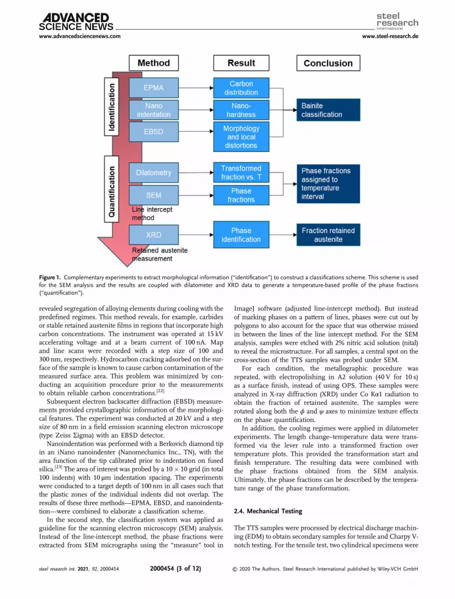
The quantification of phase fractions in the three steels wasconducted in two steps: an identification (classification) phaseand a quantification step (Figure 1). In the first step, morpholog-ical features were described by a comprehensive analysis ofdifferent experiments to extract information in the same localarea. The heat-treated samples were further processed to extractsecondary samples for metallographic preparation and mechan-ical testing. Samples were ground and polished to a surfacefinish of 1 μm. Oxide polishing suspension (OPS) made of col-loidal silica with a 0.25 μm particle size was used to obtain a sur-face with minimal roughness. This final step was chosen insteadof electropolishing to satisfy the surface requirements of electronprobe microanalysis (EPMA) and nanohardness measurementsdespite a small risk of a possible TRIP effect initiated by mechan-ical preparation. Microhardness indents were used as markers tolocate the same spot for the different experiments.

EPMA measurements in a Schottky field-emission gun elec-tron microprobe, JEOL JXA-8530 F (JEOL Ltd., Tokyo, Japan),

Table 1. Chemical composition of laboratory steels in wt%.

C Si Mn Cr Mo Nb B Ti Al S N P O

Steel 1 0.23 1.18 1.48 0.50 0.083 0.015 0.0031 0.019 0.004 0.003 0.0055 0.006 0.0021

Steel 2 0.20 1.51 1.99 0.50 0.083 0.015 0.0031 0.019 0.005 0.003 0.0059 0.006 0.0017

Steel 3 0.19 1.53 2.48 0.50 0.083 0.015 0.0031 0.020 0.005 0.003 0.0056 0.006 0.0011

www.advancedsciencenews.coml



http://www.advancedsciencenews.com


revealed segregation of alloying elements during cooling with thepredefined regimes. This method reveals, for example, carbidesor stable retained austenite films in regions that incorporate highcarbon concentrations. The instrument was operated at 15 kVaccelerating voltage and at a beam current of 100 nA. Mapand line scans were recorded with a step size of 100 and300 nm, respectively. Hydrocarbon cracking adsorbed on the sur-face of the sample is known to cause carbon contamination of themeasured surface area. This problem was minimized by con-ducting an acquisition procedure prior to the measurementsto obtain reliable carbon concentrations.[22]

Subsequent electron backscatter diffraction (EBSD) measure-ments provided crystallographic information of the morphologi-cal features. The experiment was conducted at 20 kV and a stepsize of 80 nm in a field emission scanning electron microscope(type Zeiss Σigma) with an EBSD detector.

Nanoindentation was performed with a Berkovich diamond tipin an iNano nanoindenter (Nanomechanics Inc., TN), with thearea function of the tip calibrated prior to indentation on fusedsilica.[23] The area of interest was probed by a 10� 10 grid (in total100 indents) with 10 μm indentation spacing. The experimentswere conducted to a target depth of 100 nm in all cases such thatthe plastic zones of the individual indents did not overlap. Theresults of these three methods—EPMA, EBSD, and nanoindenta-tion—were combined to elaborate a classification scheme.

In the second step, the classification system was applied asguideline for the scanning electron microscopy (SEM) analysis.Instead of the line-intercept method, the phase fractions wereextracted from SEM micrographs using the “measure” tool in

ImageJ software (adjusted line-intercept method). But insteadof marking phases on a pattern of lines, phases were cut out bypolygons to also account for the space that was otherwise missedin between the lines of the line intercept method. For the SEManalysis, samples were etched with 2% nitric acid solution (nital)to reveal the microstructure. For all samples, a central spot on thecross-section of the TTS samples was probed under SEM.

For each condition, the metallographic procedure wasrepeated, with electropolishing in A2 solution (40 V for 10 s)as a surface finish, instead of using OPS. These samples wereanalyzed in X-ray diffraction (XRD) under Co Kα1 radiation toobtain the fraction of retained austenite. The samples wererotated along both the ϕ and ψ axes to minimize texture effectson the phase quantification.

In addition, the cooling regimes were applied in dilatometerexperiments. The length change–temperature data were trans-formed via the lever rule into a transformed fraction overtemperature plots. This provided the transformation start andfinish temperature. The resulting data were combined withthe phase fractions obtained from the SEM analysis.Ultimately, the phase fractions can be described by the tempera-ture range of the phase transformation.

2.4. Mechanical Testing

The TTS samples were processed by electrical discharge machin-ing (EDM) to obtain secondary samples for tensile and Charpy V-notch testing. For the tensile test, two cylindrical specimens were

Figure 1. Complementary experiments to extract morphological information (“identification”) to construct a classifications scheme. This scheme is usedfor the SEM analysis and the results are coupled with dilatometer and XRD data to generate a temperature-based profile of the phase fractions(“quantification”).






machined per condition with a cylindrical shape of 5� 25 mm2

between the screw threads. The test was conducted usingthe tensile test machine Zwick 4204 at a constant speed of0.4mmmin�1 (strain rate of 0.00025 s�1).

From another TTS sample per condition, three subsized CharpyV-notch samples were machined with a rectangular cross-sectionof 2.5� 10mm2 and 55mm in length. Both tests were conductedat room temperature.

3. Results

A combination of carbon map (EPMA), force-depth behavior(nanohardness), band contrast, and misorienation boundaries(EBSD) was used for steel 1 in different cooling regimes.

Regime III produces a high degree of inhomogeneity.Therefore, a larger surface area was analyzed to attain more rep-resentative results (Figure 2). In the granular-type morphology,large areas of carbon depletion are visible, whereas a uniformcarbon distribution can be observed in the shape of islands witha large scattering in size. Again, the band contrast reveals a linkof highly distorted areas and high carbon concentration. Largerislands with high carbon concentration contain a carbon gradientfrom the border to the core of the island. The grain boundariesshow only a few high-angle boundaries but dominantly low-angleboundaries. Regime I and regime II were analyzed accordingly(for the images, the reader is referred to the SupportedInformation of the online version).

In regime I, carbon-enriched areas were observed alongcarbon-depleted lath, while some grains showed a homogeneouscarbon distribution. The carbon-enriched areas coincide with

regions of low distortion (dark gray scale values in the bandcontrast). Otherwise, carbon depletion can be linked to light grayscale values and therefore, microstructural constituents withlow distortion. High-angle boundaries are prevalent in regime I.Consequently, the microstructure of regime I contains ahomogeneous lath-type structure with a small fraction of highlydistorted areas, typical for morphologies transformed at lowertemperatures (i.e., fresh martensite).

In regime II, the carbon map reveals areas of carbon separa-tion by diffusion and regions of uniformly distributed carbon.The former corresponds to areas of low distortion in the bandcontrast with embedded block-type retained austenite with highcarbon concentration. Areas of uniform carbon distributionappear in dark gray scale values as an indicator for transforma-tion products that originated from low temperatures. The coarsercarbon-depleted areas result in an increase of the number oflow-angle boundaries at the cost of high-angle boundaries.

In addition to EPMA maps, line scans were obtained tomonitor the elemental changes across phase boundaries for steel1 in regimes I–III (Figure 3). In regime I, the carbon distributioncorresponds either to moderate fluctuations or regions of highcarbon concentration with high distortions. Regime II containsin addition carbon-depleted areas next to high-carbon areas withup to 0.6 wt% C. Alternating carbon depletion and high carbonconcentration can be observed in regime III, with maximum con-centrations of up to 0.9 wt% C. For other alloying elements, nodiffusion can be identified from the EPMA results, as it can beseen from regime II.

Nanohardness in regime I reflects the homogenous carbondistribution by a narrow hardness distribution with a mean hard-ness and standard deviation of 4.44� 0.74 GPa (Figure 4).

Figure 2. Left: Carbon distribution by EPMA of steel 1 in regime III (1-500-0.3) shows strong localized carbon concentrations surrounded by carbon-freeareas. Regions of elevated carbon with boundaries of high carbon indicate M–A islands. The same area was probed by nanohardness with a 10� 10 gridof indentations (indicated by red arrows). The red rectangle marks the region of the EBSD measurement. Upper right: The band contrast of this arearepresents a low degree of distortion (light gray values) in the carbon-depleted areas (retained austenite is colored in green). Lower right: The same regionobtains a high amount of low-angle boundaries in carbon-depleted areas and only a few high-angle boundaries (in red) in areas of uniform carbondistribution. A larger area was analyzed due to the strong microstructural inhomogeneity.






For regimes II and III, peak broadening can be detected with4.69� 1.16 GPa in regime II and 4.55� 1.47 GPa in regimeIII. The right column of Figure 4 shows examples of microstruc-tural categories (with fcc austenite in green) overlapped with thecorresponding nanohardness indent. The indents are classifiedinto different microstructural constituents for steel 1, separatedafter the cooling regime. The lowest hardness was measuredfor bainitic ferrite, in regimes II and III, with a correspondingmean value of 2.64� 0.81 GPa for regime III. The absence ofgranular bainite in regime I results in a higher hardness forcarbon-supersaturated lath of bainitic ferrite with a mean valueof 3.88� 0.04 GPa. Dark gray scale values in the band contrastrepresent fresh martensite. These regions yield a high nanohard-ness above 5 GPa, as it can be seen for regime III with5.53� 0.52 GPa. Retained austenite as block or film contributesto an intermediate range of hardness. During loading, a “pop-in”in the early stage of loading is seen as the result of the homoge-neous nucleation of dislocations under the indenter tip when no

sources exist due to a damage-free surface (the interpretation ofpop-ins will be further specified in the discussion). Duringunloading, an “elbow” behavior can be observed. In the litera-ture, “pop-out” or elbow behavior can be correlated with anexpansion of volume below the indenter tip due to a phase tran-sition.[24] In case of an extensive or very rapid expansion, pop-outis commonly seen for high loading rates and high maximumloads, while for a lower degree of expansion, rather an elbow-likebehavior can be observed for low loading rates and lower maxi-mum loads during indenter release. Pop-outs and elbows areboth signs of indentation-induced transformation. Pop-in behav-ior during loading was observed in retained austenite of steel 1 inregime I (Figure 5). Another indent that coincided with retainedaustenite yielded a gradient change of slope during unloading(elbow behavior).

Additional information can be extracted by the spatial correla-tion of nanohardness with the observed morphology. It becomesclear that dark gray scale values correspond to martensite and

Figure 3. IQ maps with superimposed fcc phase in green of a) regime I (1-400-0.3), b) regime II (1-500-1), and c) regime III (1-500-0.3) of steel 1.The carbon distribution is shown below the marked region. Regions 1, 2, and 3 indicate C depletion, moderate fluctuations of C, and highlyconcentrated C; other elements (Si, Cr, Mn, Mo) show no signs of diffusion.






(a)

(b)

(c)

Figure 4. Left: Broadening of nanohardness distribution in b) regime II and c) III based on steel 1, whereas nanohardness values of a) regime I areobserved in a narrow hardness distribution (each hardness distribution was fitted with a lognormal distribution function). Right: Nanohardness as a redtriangle with mean value (�standard deviation) of selected microstructural constituents according to (a–c) in steel 1 after cooling in different regimes(hardness of martensite in regime I is based only on one measurement). Green regions indicate fcc austenite; dark areas indicate highly distortedmartensite (scale bar applies for all images; red, blue, and black will be used again in Figure 5 to assign the three microstructural constituents).

Figure 5. Load–displacement behavior of selected morphologies. “pop-ins” during loading in the vicinity of retained austenite and martensite representhomogeneous nucleation of dislocations. For instance, a) block-type retained austenite in regime I as a solid line indicates homogenous nucleationof dislocations during loading. An “elbow” during unloading is caused by phase transformation. For instance, elongated retained austenite in regimeI as dashed line during unloading causes volume expansion below the indenter probably due to martensite transformation. A high scattering ofload–displacement behavior was observed for b) regime II and c) III.






bright gray values to bainitic ferrite. In addition to retained aus-tenite, the former shows occasionally an elbow behavior as anindicator of martensite transformation. Only bainitic ferriteshows an absence of such discontinuities. Furthermore, coolingregimes II and III resulted in a significant scatter of load-

displacement curves in each microstructural class, whereasthe curves almost overlap in regime I.

The previous findings were used to elaborate a classificationscheme. Afterward, the classification was applied on steel 1 indifferent regimes and on three different steels with differenthardenability levels. For the quantification of microstructures,

Table 2. Classification system for bainite microstructures in wire rod steel. An elevated carbon concentration in low-temperature morphologies refers to ahigher carbon concentration than in the overall carbon content but lower as in intermediate-temperature morphologies.

Class Morphology (SEM) Carbon concentration and distribution (EPMA) Distortions (EBSD) Hardness (nanohardness)

Low-temperature morphologies Highly refined lath Elevated C, uniformly distributed High High

Intermediate-temperature morphologies Less refined lath Peaks of high carbon concentration,high-frequency fluctuations

Intermediate Intermediate

High-temperature morphologies Granular and coarse C depletion Low Low

Figure 7. Pie charts show the phase fractions of retained austenite, low-, intermediate-, and high-temperature morphologies; a) different cooling regimesin steel 1 cause an inhomogeneous mixture of phases in regimes II and III; b) in steel 1–3, the increase of manganese causes an increasing dominance oflow-temperature morphologies.

Figure 6. Interrupted dilatometer experiment of regime II, quenched after reaching a) 470 �C containing selected high-temperature morphologiesin brown, b) 410 �C with selected intermediate-temperature morphologies in green, and c) 350 �C with low-temperature morphologies (marked inblue with primarily quenched martensite).






three classes are defined as follows: 1) high-temperature,2) intermediate-temperature, and 3) low-temperature morpholo-gies, according to differences in the morphology, carbondistribution, distortion, and hardness (Table 2).

In addition, dilatometer experiments were conducted to trackthe evolving phase transformation after interrupting the coolingat different temperatures. In the SEM micrographs afterinterrupting the cooling of regime II (Figure 6), these regionscan be differentiated by the etching response. No or lowetching response corresponds to low-temperature morphologies,whereas coarse regions with pronounced topographic effectrelate to the first class. In case of a clearly visible lath shape,the region is marked as intermediate morphology.

The results of the phase fraction analysis for different coolingconditions and three different steel compositions are shown inFigure 7. Each pie chart contains the retained austenite fractionobtained from XRD. The fraction of retained austenite lies in therange of 5.6% in regime II of steel 3 and 14.7% for regime IIIof steel 1. A change in cooling regime causes from regime Ito regime III an increase in high-temperature morphologies(in brown) on the cost of intermediate morphologies. RegimeIII displays a mixture of low- and high-temperature morpholo-gies with a low fraction of intermediate morphologies.

The effect of manganese was analyzed in regime I and II.In both regimes, the fraction of low-temperature morphologies(in blue) increases. This increase in regime I reduces the amount

Figure 8. a–c) Effect of cooling regime in steel shows primarily intermediate-temperature morphologies in regime I (0.3 K s�1 from 400 �C), whereas inregime II (1 K s�1 from 500 �C) and regime III (0.3 K s�1 from 500 �C) high-temperature morphologies dominate the microstructural composition.d–f ) Increasing the manganese content from 1.5 to 2 and 2.5 wt% causes in regime II higher fractions of low-temperature morphologies, but atthe cost of high-temperature morphologies. The same tendency was observed in regime I.






of intermediate-temperature morphologies, where no high-temperature morphologies are observed. In regime II, the rise ofblue fractions is more severe and diminishes high-temperaturemorphologies.

The phase fractions are assigned to the dilatometer data (trans-formed fraction over temperature) for cooling in regimes I–III,as shown in Figure 8a–c. The curves were obtained from thelength change data via the lever rule. Cooling in regime I gen-erates a homogeneous microstructure originated from a narrowtemperature range. At higher transformation temperatures, themicrostructure is composed of different morphologies formed ata broader temperature range. A steep transition of high- to low-temperature morphologies can be seen in regime III. It has to benoted that the phase fractions add up to 100%, indicated by they-axis. But the diagram refers to the transformation start (0%)and finish temperatures (100%) in the shown temperature range.Retained austenite is not considered in the curve as it is assumedstable at room temperature. Thus, the overall phase fractions arereduced by the amount of retained austenite.

The effect of hardenability by increased manganese contentis plotted in Figure 8d–f. The fractions of high- and intermediate-temperature morphologies (in green and blue) reduces anddiminishes at 2.5 wt% Mn in steel 3. For this steel, regimes

I and II visually almost overlap with a high fraction of low-temperature morphologies. In regime I, increasing the manganesecontent correlates to increased fractions of low-temperaturemorphologies on the cost of intermediate-temperaturemorphologies.

Table 3 provides an overview of transformed volume fractionsand the according transformation start temperatures. The effectof manganese in regime I in steel 1, 2, and 3 shows a cleardecrease of intermediate start temperatures, while the low-temperature morphologies begin to transform in the same rangeof �370 �C. The effect of manganese is more severe in regime IIby decreasing the transformation temperatures significantly andby shifting the transformation curve to lower temperatures.

The results of mechanical testing in different cooling regimesof steel 1 are summarized in Table 4. Regime I stands out withhigh strength of 953MPa [yield stress (YS)] and 1274MPa [ulti-mate tensile strength (UTS)]. This causes a high yield ratio of0.75. In addition, regime I yields the highest impact energyamong the tested conditions. Regimes II and III cause an earlyonset of plastic deformation and lower tensile strength and adeterioration of impact energy. The ductility can be increasedby regime III with 11.6% uniform elongation (UEl) and14.7% total elongation (TEl), respectively.

The mechanical properties of steel 2 and 3 with different man-ganese contents are separated into regimes I and II. In the for-mer, the increase of manganese causes higher strength but lowerimpact energy. Uniform elongation and total elongation areincreased in steel 2, while a manganese content of 2.5 wt%causes a deterioration of ductility. In regime II, a broaderrange in yield stress (YS: 785–1035MPa) and tensile strength(UTS: 1157–1552MPa) can be observed. Elongation valuesappear again higher in steel 2, whereas the impact energyincreases slightly with increasing manganese content.

4. Discussion

4.1. Microstructure–Property Relationship

The impact of the phase fractions on the mechanical propertiesat room temperature depends on the cooling parameters and thechemical composition.

Table 3. Bainite fractions in steel 1 (regimes I–III), steel 2 (regimes I–II),and steel 3 (regimes I–II) with transformation start temperatures of high-,intermediate-, and low-temperature morphologies (last column). inregime I, two classes can be observed, while high-temperaturemorphologies occur in regime II. An increase of manganese causeslower transformation temperatures, with a more severe effect in regimeII than in regime I.

Regime Low[T] [%]

Intermediate[T] [%]

High[T] [%]

Bs [�C]:low–intermediate–high

Steel 1 I 4.9 95.1 – 373–487–(–)

II 31.1 16.4 52.5 390–414–528

III 30.0 9.2 60.8 448–459–517

Steel 2 I 8.1 91.9 – 369–395–(–)

Steel 3 80.8 19.2 – 371–384–(–)

Steel 2 II 85.8 9.5 4.7 401–435–469

Steel 3 96.7 1.4 1.9 368–379–394

Table 4. Mechanical properties according to cooling regime of steel 1 and according to manganese content of steel 2 and 3 for cooling regimes I and II.

Regimea) Yield strength [MPa] Tensile strength [MPa] Yield ratio [–] UEl [%] TEl [%] CIV [ J ]

Steel 1(1.5 wt% Mn) I 953 1274 0.75 3.8 12.2 21

II 785 1157 0.68 5.1 7.5 9

III 709 1133 0.63 11.6 14.7 5

Steel 2 (2.0 wt% Mn) I 992 1394 0.71 4.8 15.5 18

Steel 3 (2.5 wt% Mn) 1068 1486 0.72 3.0 6.4 16

Steel 2 (2.0 wt% Mn) II 989 1444 0.68 3.0 8.7 14

Steel 3 (2.5 wt% Mn) 1035 1552 0.67 4.3 7.8 15

a)UEl, TEl, and CIV indicate uniform elongation, total elongation, and Charpy V-notch toughness (at room temperature), respectively. CIV values are based on the average ofthree subsized samples.






4.1.1. Effect of Cooling Regime

Slow cooling in the lower bainite phase field beginning from400 �C (regime I) produces primarily one type of bainite trans-formed in a narrow temperature range with 4% low-temperaturemorphologies. The low amount of brittle morphologies sur-rounded by a lath-shape morphology with high-angle misorien-tations causes a high yield point during tensile testing. Theabsence of granular morphologies in this regime provides arelatively high tensile strength. In this context, regime I showedthe highest impact energy among the tested steels and the EBSDresults revealed a high degree of high-angle misorientations aseffective barriers against crack propagation.[6]

At higher temperatures, a simulated air-cooling route begin-ning from 500 �C (regime II) produces a broader temperaturewindow and subsequently a mixture of morphologies dominatedby coarse high-temperature morphologies. This type of bainitecontains coarse bainitic ferrite with low-angle boundaries. Thelow strength of this particular morphology causes deteriorationof the yield stress. Together with a decrease of tensile strength, alower yield ratio of 0.68 was observed, as an indicator of anincreasingly inhomogeneous microstructure. The mixture ofmorphologies seems disadvantageous for ductility. Comparedto regime I, this regime obtains slightly more retained austenitebut the increase of low-temperature morphologies with uniformcarbon distribution provides less deformability during tensiletesting. The high degree of coarse morphologies with low-angleboundaries can be linked to low resistance against impactloads.

A further decrease of the cooling rate in the upper bainitephase field at 500 �C (regime III) introduces more retained aus-tenite (in agreement with the retained austenite measurementsin Table 5) and high-temperature morphologies at the cost of thelath-type bainite from intermediate temperatures. With a highamount of granular bainitic ferrite, yielding already occurs at709MPa. This microstructure represents the highest degree ofobserved microstructural inhomogeneity, which manifests in alow yield ratio of 0.63. The broad scattering of nanohardness con-firms this tendency. The lack of intermediate-temperature mor-phologies yields a hardness gradient from low-temperature to

high-temperature constituents. Under loading, this heterogene-ity appears critical for crack nucleation. Moreover, the observedlow-angle misorientations are responsible for the deterioration ofimpact energy. On the other hand, regime III benefits from ahigh degree of soft bainitic ferrite and retained austenite to pro-vide better ductility.

4.1.2. Effect of Manganese Content

The hardenability level can be controlled by the manganese con-tent. In regime I, the increase of manganese from 1.5 to 2.5 wt%produces a microstructure dominated by low-temperaturemorphologies. The high nanohardness in this microstructuralconstituent correlates to a higher overall strength (UTS¼ 1486MPa).In contrast, the microstructure is not suitable to provide highductility and impact toughness. The former can be explainedby a lack of softer phases with a reduced fraction of retainedaustenite and bainitic ferrite. Low temperature morphologiessuch as fresh martensite can be regarded as brittle and therefore,the impact toughness deteriorates.

With increasing manganese content, the difference in proper-ties from regime I to II becomes less significant. For instance,the difference in yield strength between regime I and II for steel1 is significantly higher, with 168MPa compared to 33MPa insteel 3. This makes steel 3 less sensitive to changes in the coolingparameters. Thus, steel 3 is more suitable for larger wire diam-eters, which are usually prone to axial temperature gradients andmicrostructural heterogeneities.

4.2. Comparison of Characterization Methods

Different methods were used to characterize the microstructureof wire rod steels. Each method contributes differently to thefinal phase quantification. For instance, in high-temperaturemorphologies, carbon maps by EPMA provide a clear distribu-tion of carbon on the sample surface in addition to the precisemeasurements of carbon concentrations via line scans of carbon.In contrast, transformation at lower temperatures causeslath-type morphologies with a lath width on the submicron level.This exceeds the resolution of EPMA to resolve fine differencesin carbon distribution. On the other hand, EPMA records linescans that can be correlated with a misorientation analysis byEBSD. Although the absolute carbon concentration in lath-typeregions seems underestimated due to an overlap of bainiticferrite and retained austenite films, EPMA is a powerful toolin extension to the averaged information of carbon concentration(provided by XRD).

Nanohardness is able to obtain mechanical properties of a sin-gle microstructural morphology. TEM observation in siliconsteels proved that the elbows and pop-outs occurring duringunloading can be linked to a phase transformation.[25] The vol-ume expansion by transformation causes an uplift of theindenter tip. In case of pop-out, this uplift takes place abruptly,promoted by higher maximum loads and increased (un-)loadingrates. Otherwise the elbow-like gradual change in the unloadingcurve is the result of a phase transformation with a lower volumeexpansion, for example, at lower maximum loads and loadingrates. And in fact, the discontinuities were observed in the

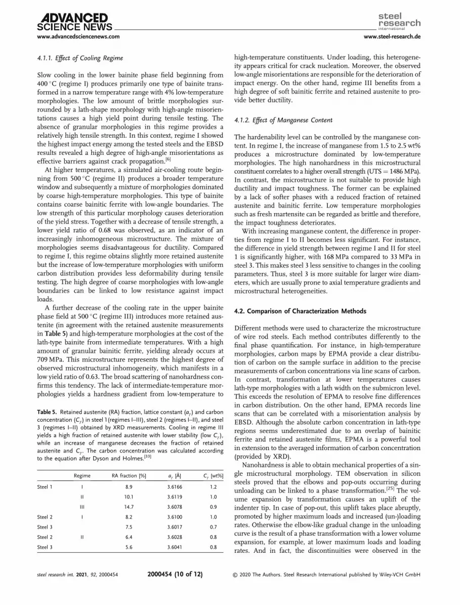
Table 5. Retained austenite (RA) fraction, lattice constant (aγ) and carbonconcentration (Cγ) in steel 1(regimes I–III), steel 2 (regimes I–II), and steel3 (regimes I–II) obtained by XRD measurements. Cooling in regime IIIyields a high fraction of retained austenite with lower stability (low Cγ),while an increase of manganese decreases the fraction of retainedaustenite and Cγ . The carbon concentration was calculated accordingto the equation after Dyson and Holmes.[33]

Regime RA fraction [%] aγ [Å] Cγ [wt%]

Steel 1 I 8.9 3.6166 1.2

II 10.1 3.6119 1.0

III 14.7 3.6078 0.9

Steel 2 I 8.2 3.6100 1.0

Steel 3 7.5 3.6017 0.7

Steel 2 II 6.4 3.6028 0.8

Steel 3 5.6 3.6041 0.8






vicinity of martensite and the retained austenite—i.e., where aTRIP effect would be expected—and not near the bainitic ferrite.

Discontinuities are seen in the indentation load–displacementcurves both in the loading data (as pop-ins) and in the unloadingdata (as elbows). In the literature, pop-ins during the testing ofsimilar steels have been linked to a phase change via a TRIPeffect,[26–28] and in some cases this has also been confirmedby TEM.[27,28] However, such pop-ins are also commonly associ-ated with the homogenous nucleation of dislocations underneaththe sharp indenter tip,[29–31] and therefore in this work it cannotbe unambiguously said to which mechanism these featuresbelong. However, the additional “elbow-ing” in the unloadingcurve has also been shown to be associated with a phase trans-formation.[29,32] This, in conjunction with the fact that these dis-continuities were observed in the vicinity of martensite and theretained austenite—i.e., where a TRIP effect would be expected—and not near the bainitic ferrite, therefore, strongly impliesthey are a result of a TRIP effect also occurring here. A morepronounced elbow was observed in the martensitic morphologyof regime III compared to the retained austenite. Thus, it can beassumed that retained austenite facilitates dislocation move-ments during phase transformation, which can be seen by adamped elbow in contrast to an indentation-induced transforma-tion with adjacent martensite. In summary, nanohardness is apowerful tool to gain further insights into the microstructuralhomogeneity, given a sufficient number of indents. But the fullpotential of nanohardness is reached by coupling this techniquewith EBSD and EPMA. The local information of the localcarbon concentration, nanohardness, and misorienation pro-vides complementary information on the microstructuralconstituents.

5. Conclusion

The carbide-free bainite concept was tested on three steels withdifferent manganese contents and three different coolingregimes, according to the process window of a wire rod coolingconveyor. Different characterization methods were combined toreveal the effect of varied cooling parameters and hardenabilitylevel on the microstructure. In summary, the findings are asfollows. 1) The change of cooling regime causes significantdifferences in the bainite morphology. The comprehensive useof EBSD, EPMA, and nanohardness is suitable to monitor andcategorize these differences. Merging the results of the adjustedline-intercept method, XRD, and dilatometry yields a quantifica-tion of the microstructural features. 2) A classification based onEPMA or nanohardness alone is not sufficient. Only a combina-tion of these techniques with EBSD provides enough informa-tion for classifying bainite in wire rod steel. The results wereused to classify the microstructure into three classes: low-, inter-mediate-, and high-temperature morphologies. 3) The coolingrate in the bainite phase field has an impact on the homogeneityof the final microstructure. At 400 �C, a relatively low cooling rateto 0.3 K s�1 causes a homogeneous microstructure primarilycomposed of intermediate-temperature morphologies. In con-trast, simulated air cooling of 1 K s�1 at 500 �C causes a mixtureof all three microstructural classes. Cooling from 500 �C with0.3 K s�1 develops a granular microstructure with primarily

low- and high-temperature morphologies with a steep hardnessgradient. 4) Nanohardness measurements are suitable to revealmicroscopic properties of microstructural features. The retainedaustenite shows linkages to elbows in the load–displacementcurves during unloading as an indicator of martensite transfor-mation beneath the indenter tip, whereas pop-ins during loadingcannot be unambiguously interpreted. 5) Regarding the macro-scopic mechanical properties, high-temperature morphologiescontain relatively high amounts of ferrite and retained austenite,which in turn have a beneficial effect on ductility. A steephardness gradient for a mixture of low- and high-temperaturemorphologies facilitates crack propagation and thus, yields lowimpact energies. 6) An increase of manganese content from1.5 to 2.5 wt% has an impact on the resulting microstructureand properties. For 2.5 wt% Mn, changes in the cooling regimebecome more negligible. Thus, manganese causes a lowersensitivity to the cooling regime. This makes higher manganesecontents attractive for larger wire diameters, which are prone totemperature gradients in axial direction during cooling.

AcknowledgementsThe work was done in the framework of a collaboration project withArcelorMittal Maizières, Research and Development Bars and Wires, aspart of the knowledge-building program at ArcelorMittal. Open accessfunding enabled and organized by Projekt DEAL.

Conflict of InterestThe authors declare no conflict of interest.

Keywordscarbide-free bainite, classification, microstructures, wire rod steel

Received: August 20, 2020Revised: September 23, 2020

Published online: October 25, 2020

[1] M. Takahashi, H. K. D. H. Bhadeshia, Mater. Sci. Technol. 1990, 6,592.

[2] S. Zajac, S. Komenda, P. Morris, P. Dierickx, S. Matera, F. PenalbaDiaz. Quantitative Structure–Property Relationships for ComplexBainitic Microstructures. Final Report. EUR Technical SteelResearch – Physical Metallurgy and Design of New Generic SteelGrades EUR-21245-EN, Luxembourg, 2005.

[3] S. Zajac, V. Schwinn, K. H. Tacke, Mater. Sci. Forum 2005, 500, 387.[4] B. L. Bramfitt, J. G. Speer, Metall Trans A 1990, 21, 817.[5] K.-I. Sugimouto, T. Iida, J. Sakaguchi, T. Kashima, ISIJ Int. 2000, 40,

902.[6] F. G. Caballero, H. Roelofs, S. Hasler, C. Capdevila, J. Chao,

J. Cornide, C. Garcia-Mateo, Mater. Sci. Technol. 2013, 28, 195.[7] F. G. Caballero, H. K. D. H. Bhadeshia, Curr. Opin. Solid State Mater.

Sci. 2004, 8, 251.[8] X. Y. Long, F. C. Zhang, J. Kang, B. Lv, X. B. Shi, Mater. Sci. Eng. A

2014, 594, 344.[9] T. Sourmail, C. Garcia-Mateo, F. Caballero, L. Morales-Rivas,

R. Rementeria, M. Kuntz, Metals 2017, 7, 31.






[10] I. Jain, S. Lenka, S. K. Ajmani, S. Kundu, J. Thermal Sci. Eng. Appl.2016, 8, 1129.

[11] P. Janssen, Wire J. Int. 2014, 47, 60.[12] F. G. Caballero, H. K. D. H. Bhadeshia, Mater. Sci. Forum. 2003, 426,

1337.[13] C. Hofer, H. Leitner, F. Winkelhofer, H. Clemens, S. Primig, Mater.

Character. 2015, 102, 85.[14] C. Hofer, F. Winkelhofer, H. Clemens, S. Primig, Mater. Sci. Eng. A.

2016, 664, 236.[15] L. Guo, H. Roelofs, M. I. Lembke, H. K. D. H. Bhadeshia, Mater. Sci.

Technol. 2017, 34, 54.[16] B. P. J. Sandvik, H. P. Nevalainen, Metals Technol. 1981, 8, 1213.[17] A. Lambert, J. Drillet, A. F. Gourgues, T. Sturel, A. Pineau, Sci. Technol.

Weld. Join. 2013, 5, 168.[18] P. Jacques, F. Delannay, X. Cornet, P. Harlet, J. Ladriere, Metall.

Mater. Trans. A. 1998, 29, 2383.[19] K.-I. Sugimouto, R. Kikuchi, S.-I. Hashimoto. Steel Res. 2002, 73, 253.[20] K. Zhu, C. Oberbillig, C. Musik, D. Loison, T. Iung, Mater. Sci. Eng. A

2011, 528, 4222.[21] S. Y. Han, S. Y. Shin, C.-H. Seo, H. Lee, J.-H. Bae, K. Kim, S. Lee,

N. J. Kim, Metall. Mater. Trans. A 2009, 40, 1851.

[22] P. T. Pinard, A. Schwedt, A. Ramazani, U. Prahl, S. Richter, Microsc.Microanal. 2013, 19, 996.

[23] W. C. Oliver, G. M. Pharr. J. Mater. Res. 1992, 7, 1564.[24] M. Aarnst, Microstructural Quantification of Multi Phase

Steels-MICRO-QUANT, 2009.[25] V. Domnich, Y. Gogotsi, S. Dub, Appl. Phys. Lett. 2000, 76,

2214.[26] B. B. He, M. X. Huang, Z. Y. Liang, A.H.W. Ngan, H. W. Luo, J. Shi,

W. Q. Cao, H. Dong. Script Mater. 2013, 69, 215.[27] T.-H. Ahn, C.-S. Oh, D. H. Kim, K. H. Oh, H. Bei, E. P. George,

H. N. Han, Script Mater. 2010, 63, 540.[28] Z. Xiong, G. Casillas, A. A. Saleh, S. Cui, E. V. Pereloma, Sci. Rep.

2017, 7, 17397.[29] R. Rao, J. E. Bradby, S. Ruffell, J. S. Williams, Microelectron. J. 2007,

38, 722.[30] C. A. Schuh, Mater. Today 2006, 9, 32.[31] R. Navamathavan, S.-J. Park, J.-H. Hahn, C. K. Choi,Mater. Character.

2008, 59, 359.[32] J.-I. Jang, M. J. Lance, S. Wen, T. Y. Tsui, G. M. Pharr, Acta Mater.

2005, 53, 1759.[33] D. J. Dyson, B. Holmes, J. Iron Steel Inst. 1970, 469.






methods to classify bainite in wire rod steel

Documents